1

POSITIVE PROFITS AND POSITIVE SURPLUS LABOUR

Gustavo Lucas*

Franklin Serrano*

Abstract

Steedman (1975) has provided an example of a pure joint production system (without fixed

capital or land) in which the rate of profits and their associated prices of production were

positive and yet aggregate “surplus value” was negative. This example sparked a controversy

related to the questions of how to define labour values in the context of joint production and,

particularly, whether or not it implied a refutation of the so-called “fundamental Marxian

theorem”. In this paper we use Steedman´s original numerical example as basis to discuss and

clarify the economic meaning of the original example and of the subsequent literature. We

conclude that although some individual commodities may have negative labour values, using a

method proposed by Akyüz (1983) it is always possible to find an economically meaningful and

positive measure for the labour value of the aggregate surplus product (surplus value) based

only on the methods in use.

Key-words: surplus value, labour value, rate of profit, joint production

JEL classification: B51, D57, E11

Address for correspondence:

emails: gustavodlucas@gmail.com, franklinserrano@gmail.com

*Institute of Economics, Federal University of Rio de Janeiro.

I. INTRODUCTION

In an article published in the Economic Journal in 1975 Ian Steedman gave an example

of a pure joint production system (i.e., without fixed capital or land) in which the rate of

profits and their associated prices of production were positive and yet aggregate

“surplus value” was negative. This example sparked a controversy related to the

questions of how to define labour values in the context of joint production and

particularly whether or not it implied a refutation of the so-called “fundamental Marxian

2

theorem”. This “theorem” states that a positive “rate of surplus value” – the ratio

between the quantity of embodied labour on the physical surplus (“surplus value”) and

the quantity of embodied labour in the necessary consumption of workers (“variable

capital”) - is a necessary and sufficient condition for a positive general rate of profits.

Many authors tried to get around Steedman´s critique through redefinitions of the labour

values of single commodities, arguments about heterogeneous labour and considerations

about the problem of choice of technique. Few contributors, however, discussed the

actual economic meaning and relevance of the special assumptions in Steedman´s

example.

In this paper we try to do that by a critical survey and a theoretical evaluation of

this literature. We make use of Steedman´s original numerical example as basis to

compare and contrast the different contributions. Our main conclusions are that

although labour values for some single commodities can indeed be negative in the most

general case (it may happen if the system is not “all-productive”), the basic and sensible

classical proposition that in the aggregate less labour would be necessary to produce

only the necessary wage basket than to meet also the total final demand coming from

the expenditures of the capitalists always holds, even if in some cases (as in the

particular economic system depicted by Steedman) producing the necessary wage

basket could entail also jointly producing some extra outputs unneeded by the workers.

Using a method proposed by Akyüz (1983), it will be shown that it is always

possible to find an economically meaningful (i.e., that only deals with non-negative

levels of activity) amount of aggregate surplus labour for the economy without

changing the processes in use (i.e., using the dominant techniques in use in the square

system). As it will be seen, this method seems to be the only available one which is

3

coherent with the idea of taking as given the processes of production in use to measure

the aggregate amount of surplus labour.

The paper is organized as follows. Section II briefly discusses issues related to

labour values in the context of joint production since Sraffa. Section III presents and

discusses Steedman´s assumptions and results. Section IV reviews the debate on

positive profits and negative surplus value. Section V offers concluding remarks.

II. LABOUR VALUES AND JOINT PRODUCTION

Labour values, in the case of homogeneous labor, are the physical quantities of labour

directly and indirectly necessary to produce a unit of a particular commodity using the

dominant (or socially necessary) methods of production actually in use. As it is well

known, Sraffa (1960) has shown, for single production systems, that the set of prices of

production measure in labour commanded (i.e., divided by the money wage) coincide

with the set of labour values when the rate of profits is zero.

In the general case of joint production Sraffa points out that there is naturally an

obvious difficulty in thinking of what is the quantity of labour directly and indirectly

necessary to produce a particular single commodity, since more than one commodity

can be produced by the same process and at the same time that same commodity may be

produced by other processes of production.

Some authors such as Schefold (1989) have claimed that the old classical

economists and Marx implicitly only thought of single production. But this is clearly a

bit exaggerated and difficult to square with the evidence that classical economists dealt

with at least some special cases of joint product systems such as differential rent, the

4

treatment of fixed capital as a joint products and even some notions of free disposal and

the analysis of industrial byproducts1.

It is probably more reasonable to think that, while classical economists did

discuss some aspects of joint production, they overwhelmingly seem to have assumed

that, even if some elements of joint products were present, it was usually possible to

produce single commodities separately, i.e., to increase the net output of a particular

commodity without necessarily increasing the net output of any other2.

As we now know, in general joint product systems in which this is possible, it

also possible to calculate precisely what is the quantity of labour directly necessary to

produce only a unit of that particular commodity and thus there is no difficulty in

calculating its positive and additive labour value.

The difficulties with the concept of labour value of individual commodities thus

seem to be related only to systems in which production is not separable. And in general

the necessary (but not always sufficient) condition for non separability is that there are

processes in use that produce net outputs of more than one commodity. That seems to

be why simple systems with non-shiftable fixed capital or the analysis of land and

differential rents tend to behave like single product systems. Things thus tend to get

more complicated within pure joint product systems that do not possess the property of

separability.

In these type of systems Sraffa (1960, paragraph 70) has shown that the labour

values of individual commodities could turn out to be negative. Sraffa explains the

1 On fixed capital as a joint product in the classical economists and Marx see Gehrke (2012). On pure

joint production in the work of the old classical economists and Marx see Kurz (1986).

2 These systems are variedly known as “all-productive” (Schefold, 1978), or having “weak joint

production” (Abraham-Fois & Berrebi, 1997), or having the “adjustment” property, and by adding the

assumption of constant returns to scale also, as having the “non-substitution” property (Bidard &

Erreygers, 1998).

5

meaning of such negative labour values by referring to the fact that labour values are

one and the same thing as the employment multipliers of a single commodity associated

to that system of production. A negative labour value thus means that if we think of

increasing the net product of only that particular commodity by one unity, and

production is not separable and thus we will also increase the net output of at least one

other commodity, we will necessarily have to increase the amount of labour employed

by one process but also will have to decrease the level of employment in at least some

other process to prevent the overproduction of the second commodity. Now depending

on the direct amount of labour employed in the process that is expanded compared with

the process that is contracted, it may happen that in the end the total amount of labour

employed in all processes will be lower than it was before the increased of the net

output of the first commodity. In this case the commodity in question will have a

negative labour value because an increase in its production has led to a decrease in total

(direct and indirect) employment.

Moreover, Sraffa also warned in a footnote3 of the possibility of the awkward

occurrence of what he called “negative industries” by which he meant that the fact that

since under joint production the activity levels of some processes must be decreased

when that of the others increase to match the level of composition of the “requirements

of use” it was logically possible, if the change in the level and structure of demand was

sufficiently drastic, that the contraction of some particular joint processes of production

could be so extreme as to require it to be activated at a negative level.

III. STEEDMAN´S NUMERICAL EXAMPLE

3 Sraffa (1960, footnote 1, paragraph 66).

6

Steedman (1975) seems to have taken this route and, by inverting the assumptions that

Sraffa used to rule out processes with negative activity levels, produced his own

particular example. The controversy after the publication of the “positive profits with

negative surplus value” example seems to have been due to the combination of two

main factors. The first is that Steedman did not give much explanation of the economic

meaning of his results nor of the relevance of its assumptions. On the other hand, with

very few exceptions, his critics seemed so concerned to “defend” the labour theory of

value in some form that they tended mostly to add further ad hoc assumptions to those

of Steedman´s example in order to change its conclusions, instead of trying to

understand the nature of the example and its implications.

Steedman (1975, p.115) assumes an economy capable of producing a surplus of

two commodities using two joint production processes that use only circulating capital:

INPUTS OUTPUTS

commodity 1 commodity 2 labour commodity 1 commodity 2

5 0 1 6 1

0 10 1 3 12

He also assumes that the wage is paid at the end of the production period and that the

real wage basket is exogenously given: b= (0.5, 0.83). This assumption is not necessary

for the present purposes – it does not matter for the results if it is paid ex-ante or ex-

post.

The really crucial assumptions implicit in his analysis amount to three:

(i) A two commodities square system in which both processes generate the same joint

products.

7

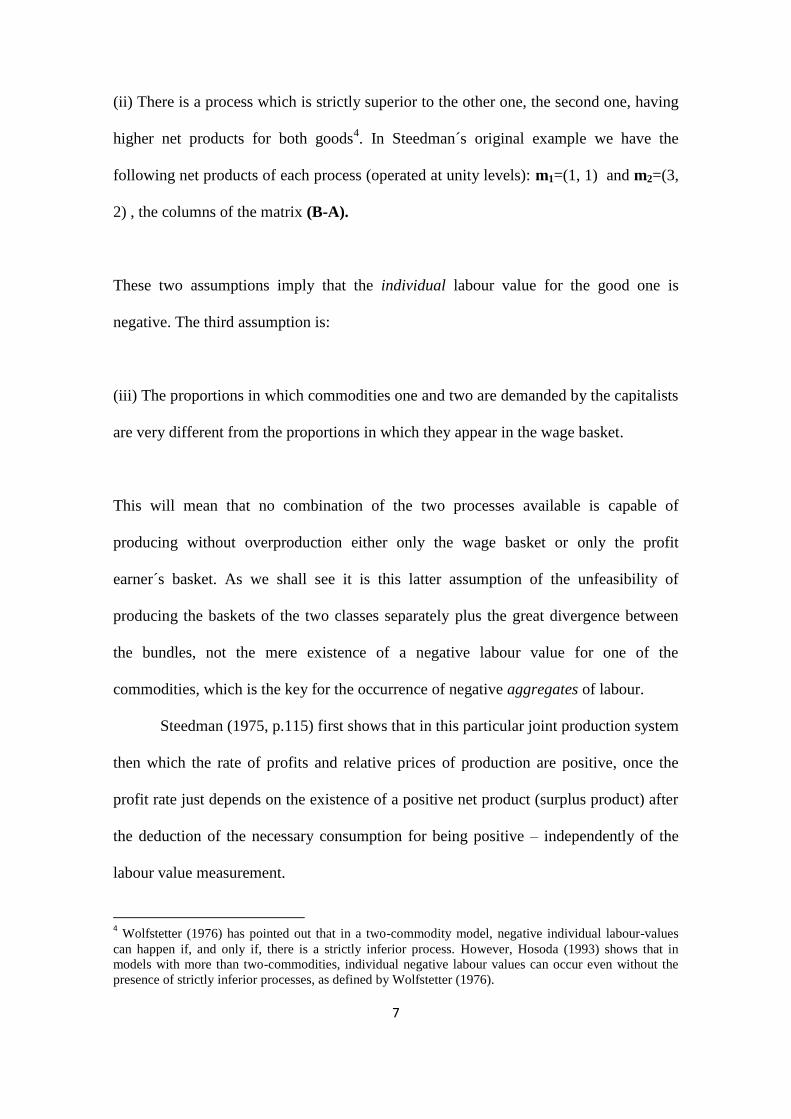
(ii) There is a process which is strictly superior to the other one, the second one, having

higher net products for both goods4. In Steedman´s original example we have the

following net products of each process (operated at unity levels): m1=(1, 1) and m2=(3,

2) , the columns of the matrix (B-A).

These two assumptions imply that the individual labour value for the good one is

negative. The third assumption is:

(iii) The proportions in which commodities one and two are demanded by the capitalists

are very different from the proportions in which they appear in the wage basket.

This will mean that no combination of the two processes available is capable of

producing without overproduction either only the wage basket or only the profit

earner´s basket. As we shall see it is this latter assumption of the unfeasibility of

producing the baskets of the two classes separately plus the great divergence between

the bundles, not the mere existence of a negative labour value for one of the

commodities, which is the key for the occurrence of negative aggregates of labour.

Steedman (1975, p.115) first shows that in this particular joint production system

then which the rate of profits and relative prices of production are positive, once the

profit rate just depends on the existence of a positive net product (surplus product) after

the deduction of the necessary consumption for being positive – independently of the

labour value measurement.

4 Wolfstetter (1976) has pointed out that in a two-commodity model, negative individual labour-values

can happen if, and only if, there is a strictly inferior process. However, Hosoda (1993) shows that in

models with more than two-commodities, individual negative labour values can occur even without the

presence of strictly inferior processes, as defined by Wolfstetter (1976).

8

From that, he shows that one of the two commodities has a negative labour

value:

(1) 1 1 2

2 1 2

5 1 6

10 1 3 12

Where 1 and

2 are the labour values of each commodity. The solution of this system

gives us the following vector of labour values:

(2) 1 2( , ) ( 1,2) -1

LΛ = a (B-A)

Where aL is the vector of direct labour requirements (composed only by units, given the

normalization presented in the table above) and is the vector of labour values (which

also correspond to the relative prices associated to the profit rate equal to zero using the

wage rate to normalize them)

Then he moves on to show also that the aggregate amount of surplus value in

this system is negative, both measured as the aggregate labour value of the sum of

commodities demanded by the capitalists and as the difference of total labour employed

versus the aggregate labour employed (embodied) in the wage basket.

The total net product is y is the sum of each class bundle yk = (5, 2) which is the

final demand which is appropriated by the capitalists, and, yw = (3, 5), the workers´

consumption.

To produce this final demand

(3) (8,7)y = (B- A)x

9

a feasible combination of both processes is required:

(4) 1 2

1 2

3 8

2 7

x x

x x

Where x1 and x2 are the levels of activity of each process required to produce the net

product (the components of vector of activity levels). The solution of this system gives

the following vector:

(5) (5,1)-1x = (B - A) y

The aggregate amount of labour is given by the sum of each element of activity level

vector using this normalization:

(6) 1 2 6L x x La x

If we multiply the final demand baskets of each class by the labour values of each

commodity, this particular technology and pattern of final demand will give us the

following labour value aggregates:

(7)

( 1).3 (2).5 7

( 1).5 (2).2 1

V

S

-1

w L w

-1

k L k

Λy = a B -A y

Λy = a B -A y

10

Where S is the surplus value and V is the variable capital. The other way for

calculating the surplus value is looking at the difference between the living labour (6

units) and the variable capital (7 units):

(8) 6 7 1S L V

Before moving on, we think that we can understand this result better if we make

the calculation in terms of activity levels associated to the production of each bundle,

instead of just finding the labour value of each bundle, as we have done for the whole

net product above. For the workers´ bundle

(9) yw = (B-A)xw= (3,5)

we need to solve:

(10) 1 2

1 2

3 3

2 5

w w

w w

x x

x x

Which gives us the following “activity levels” required to produce workers´

consumption:

(11) (9, 2) -1

w wx (B- A) y

11

The sum of each component of xw gives us the variable capital5. Applying the same

procedure for the capitalists´ bundle we get:

(12) ( 4,3) -1

k kx (B- A) y

Thus, the surplus value S can be calculated from the sum of the components xk.

This way of calculating shows that both bundles require negative activity levels

of one of the processes because both bundles cannot be produced separately by the

processes in use6.

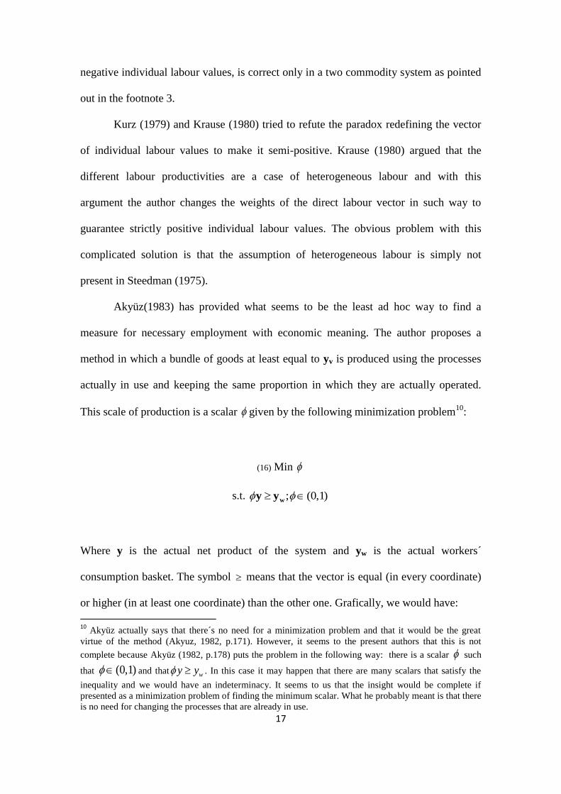
Grafically, we have that:

5 Steedman (1977, p.159) and Kurz (1979, p.68) also point out the fact that negative levels of activity are

“required” to produce separately the workers´ bundle. 6 It means that if the final demand were one of these bundles alone, the choice of technique would have to

change because it would be inefficient to match these final demands using the same square system.

12

The dotted lines provide the set (“cone”) of feasible net products using the two

processes given by the vectors m1 e m2. The horizontal axis represents the net product

of first commodity and the vertical axis the the net product of the second commodity.

As we can see, the total final demand y falls inside the cone, which means that it

can be reached with non-negative levels of activity. The total employment required for

that is 6 units. However, the bundles that each class receives fall outside the cone. This

means that they cannot be produced separately – though it is feasible to produce both

jointly. The consequence of this is that negative levels of activity are required to

produce only workers consumption or only the final demand of capitalists. If both

bundles were inside the cone no negative surplus value could happen, although the

yk

y = yk+ yw

yw

m1

m2

2 10,5y y

2

1

13

labour value of one of the two commodities would still be negative. Indeed, with the

same aggregate final demand y=(8, 7) but with the consumption of the workers being

yw=(3, 2.5) and the expenditures of the capitalists being yk=(5, 4.5), for example, we

would still get, overall activity levels x=(5, 1), total employment L=6. But now xk=(3.5,

0.5) and thus S= 3.5+0.5=4 and surplus value would be positive. For the workers we

would have xw = (1.5, 0.5) and V=2 and thus S= 6- 2=4.

In the example for the capitalists´ bundle we have that the total employment

required to produce it is negative, i.e., negative surplus value. So, we may say that

within the group of final demands that are non-feasible, there is a group which

“requires” negative amount of employment for being produced, which in this numerical

example7 are those ones that lie below the line y2=0,5y1. But the central point we want

to emphasize is that any final demand outside the cone is economically meaningless8.

We can thus see that the existence of negative labour values for single

commodities doesn´t by itself imply the paradox. The paradox of positive profits and

negative surplus value provided by Steedman (1975) rests on the fact that negative

levels of activity would be required if the bundles were to be produced separately – or,

that these bundles can only be produced jointly within this square system.

Of course negative activity levels do not exist. They are just the mathematical

symptom of the fact that there would be overproduction of one of the two commodities

if we were to produce only the wage bundle of the workers using these two processes.

So the right conclusion from Steedman´s example is that in general joint production

7 The sufficient conditions for a bundle to have negative aggregate amount of employment in a general

two commodity system (that is, being below the line in the graph) and its economic meaning are derived

in the appendix. 8 For example, if the final demands were yk=(5, 3) and yw=(3, 4), we would have positive values for S and

V, the same total employment of 6 units and it would seem that no paradox happens. However, both

bundles fall outside the cone – activity levels would be xk=(-1, 2) and xw=(6, -1) - which means that,

despite being positive, either variable capital or surplus value have no economic meaning.

14

systems the calculation of aggregate surplus labour should be adapted to deal with the

possibility of notional overproduction, instead of the economically meaningless notion

of negative activity levels

IV. SURPLUS VALUE AFTER STEEDMAN

An initial reaction to the Steedman´s example came from Morishima (1976).

Based on his earlier works such as Morishima (1973) and Morishima (1974), the author

proposed to redefine the labour values in joint production using what he calls the “true

values”. The “true value” of a commodity (or a bundle) is given by the minimization of

labour-time required to produce one net unity of it. Be ie the column vector in which

the i-th coordinate is unity and the other ones are null, the true-value of the commodity i

will be given by the following minimization problem:

(13) min. La x

s.t. iBx Ax e , x 0

Where activity levels and the processes in use are the endogenous variables of the

problem9

and the symbol means that the vector is equal or higher than the other one.

To find the “true variable capital” ei must be substituted by yw, which is going to be the

total employment required to produce workers´ consumption which minimizes the

amount of labour expended.

9 Matrixes A and B may not be square in the general case discussed by Morishima (1974)

15

Be xw* the activity levels that solves the problem, the “true variable capital”

would be:

(14) *V L wa x *

And the “true surplus value”:

(15) * *S L V

Using Steedman´s example, graphically it would be:

Where yw* is the net product associated with the level of activity xw*.

In this case, only the process with higher productivity would be operated (this is

why yw* lies above the same line as m2). Because operating this process alone cannot

produce exactly the workers´ consumption, there would be excess production of the first

yk

yw

m2

yw*

2

y = yw+ yk

“Overproduction” 1

16

commodity of 4,5 units. But the point is that less labour than the total employment

would be required to produce workers´ consumption. To produce yw=(3, 5) it would be

necessary to operate only the second processes with 2,5 units of labour. This gives a

positive “true surplus value” of 6-2,5=3,5.

The criticisms of this procedure are not new: “true-values” are not additive like

in Marx, i.e., the “true-value” of a bundle of commodities is not equal to the sum of

“true-values” of the same commodities separately produced. The authors argue that this

different definition of labour value would have a textual basis in Marx but the argument

is not very convicing (Steedman, 1976a). A second important criticism is that in this

case the (redefined) surplus value would be related to a non-capitalist (i.e., nonprofit-

maximizing) criterion for the choice of technique – while in Marx and in the literature

related to the “fundamental marxian theorem” this was based on the processes in use in

capitalism (“the socially necessary techniques”) (Akyuz, 1983). In fact the “true value”

calculations measure the hypothetical minimum amount of labour that would be

necessary to produce the wage basket for society as such and not the amount that is

“socially necessary” given the techniques and processes actually already chosen by a

capitalist criterion of choice of technique.

Wolfstetter (1976) basically questioned Steedman´s use of Sraffa´s approach of

assuming square joint production systems with equalities, instead of starting from Von

Neumann´s method of rectangular systems and using inequalities. Steedman (1976b)

promptly replied that in the particular case of his example the difference between the

two methods would hardly matter for his results, the solution being exactly the same for

both approaches. Besides, the author´s third theorem (Wolfstetter, 1976, p.867), which

states that the existence of an inferior process is a necessary and sufficient condition for

17

negative individual labour values, is correct only in a two commodity system as pointed

out in the footnote 3.

Kurz (1979) and Krause (1980) tried to refute the paradox redefining the vector

of individual labour values to make it semi-positive. Krause (1980) argued that the

different labour productivities are a case of heterogeneous labour and with this

argument the author changes the weights of the direct labour vector in such way to

guarantee strictly positive individual labour values. The obvious problem with this

complicated solution is that the assumption of heterogeneous labour is simply not

present in Steedman (1975).

Akyüz(1983) has provided what seems to be the least ad hoc way to find a

measure for necessary employment with economic meaning. The author proposes a

method in which a bundle of goods at least equal to yv is produced using the processes

actually in use and keeping the same proportion in which they are actually operated.

This scale of production is a scalar given by the following minimization problem10

:

(16) Min

s.t. ; (0,1) wy y

Where y is the actual net product of the system and yw is the actual workers´

consumption basket. The symbol means that the vector is equal (in every coordinate)

or higher (in at least one coordinate) than the other one. Grafically, we would have:

10

Akyüz actually says that there´s no need for a minimization problem and that it would be the great

virtue of the method (Akyuz, 1982, p.171). However, it seems to the present authors that this is not

complete because Akyüz (1982, p.178) puts the problem in the following way: there is a scalar such

that (0,1) and that wy y . In this case it may happen that there are many scalars that satisfy the

inequality and we would have an indeterminacy. It seems to us that the insight would be complete if

presented as a minimization problem of finding the minimum scalar. What he probably meant is that there

is no need for changing the processes that are already in use.

18

We can see that the vector falls inside the cone and, consequently, a positive

amount of employment is required to produce it. In this case, we would have a redefined

vector of workers´ consumption which has the advantage of being based in the

processes actually in use and keeping the same proportion in which they are actually

operated. This redefined surplus value S’ will be given by:

(17) ' (1 )S L

If we make a comparison with the “true-values” we can see that this method

requires much less new information and is much closer to the actual system data than

the former. In the procedure proposed by Morishima (1976) the processes and their

yk

y = yw+ yk

yw

m1

m2

y

“Overproduction” 1

2

19

relative levels of activity are altered (besides the presence of non-profit maximizing

criterion for the choice of technique). In the method proposed by Akyüz(1983) there´s

only the scalar as novelty and no change in the choice of techniques is required.

Inevitably (as in the “true-value” approach) there´s some excess of production – of the

first commodity (2,174 units in the example).

In any case Akyuz´s method allows us to see that the classical proposition that

(without changing the actual processes that are in use in a capitalists) workers

obviously work more than they would need to produce only (at least) what is contained

in their wage basket. This proportion relating positive profits and positive surplus labour

is of general validity with or without joint production, and whatever may be happening

to the labour value of individual commodities. It is important to point out that this

“overproduction” is not something that will or even may actually happen in this

economy. The term means only that this excess would happen if the system were to

produce these different quantities using the same techniques. But this is not the case

and both Akyüz or Morishima´s calculations are just like Sraffa´s standard system:

abstractions that reveal some important properties of the actual system – in our case,

the possibility of finding an economically meaningful measure of aggregate surplus

value. The calculations only provide a useful piece of information: how much labour

would be needed to produce with minimum waste the workers´ consumption basket.

Flaschel (1983, p.437) adds relative prices to the definition of individual labour

value in order to get positive magnitudes for the latter. This seems to be a contradiction

with the original function of the labour values of being a measure of physical costs,

independent from (and a major determinant of) income distribution and relative prices

More recently Trigg and Philp (2008) have claimed that there will always be

positive surplus value in aggregate even in the presence of individual negative labour

20

values for single commodities. Based in our argument, it seems that Trigg & Philp

(2008) implicitly assume that the wage basket falls inside the “cone” and thus see no

problem in calculating positive surplus labour – otherwise the Steedman´s paradox

could happen. In other words, they seem to assume that their system can produce

separately the wage basket through a combination of strictly positive activity levels of

the processes of production in use but such assumption should be made explicit to show

the logical limits of the validity of their analysis.

V. CONCLUDING REMARKS

The present work has proposed to give a clarification of the economic properties behind

the “positive profits with negative surplus value” example provided by Steedman

(1975). Criticisms such as the lack of economic meaning of the presence of an inferior

process seem quite misleading because the negative marxian aggregates are not a direct

consequence of it11

.

Individual negative labour values are certainly a necessary condition for the

paradox to happen but the central point seems to be the fact that the bundles that go to

each class must: (i) fall outside the cone given by the square system and (ii) have a very

different composition. So, the negative surplus value of the example is related to the

fact that negative levels of activity would be “required” to produce only (with no

overproduction) the capitalists´ bundle – something that is devoid of economic

meaning.

11

As pointed out in the footnote 2, although the existence of inferior process is a sufficient condition for

individual negative labour values to occur (in 2x2 is a necessary and sufficient condition), it may happen

also in other cases (Hosoda, 1993).

21

As the alternative provided by Morishima´s true values doesn´t seem useful as

being too “normative” we think that the method provided by Akyüz(1983) seems to be

the simplest and least arbitrary way to get an economically meaningful measure of

surplus labour in this case. The procedure has the advantage of using only data from the

methods that are actually in use as opposed to the literature on the so called

“fundamental Marxian theorem”.

Akyuz´s method surely seems a possible way to relate positive profits with

aggregate surplus labour but it is still true that it is still a bit cumbersome in cases like

the one used in Steedman´s example because of the unavoidable issue of notional

overproduction12

. Perhaps these complications were behind Sraffa´s (1960) procedure of

abandoning all labour embodied measures and using the amount of labour commanded

by his “standard net product” when trying to connect the rate of profits, the physical

surplus and aggregate labour in his own book. But that is another story.

REFERENCES

Abraham-Frois, G. & Berrebi, E. 1997. Prices, profits and rythms of accumulation,

Cambridge University Press

Akyüz, Y. 1983, Value and exploitation under joint production, Australian Economic

Papers, 22: 171–179

Bidard, C. & Erreygers, G. 1998. Sraffa and Leontief on Joint Production, Review of

Political Economy, vol. 10, no. 4, October, pp. 427-446

12 Some may argue that this method is not “general” in a purely mathematical sense: for example, if we

had a final demand of (9, 4) and workers´ consumption of (1, 4) there would be no solution because the

scalar that would solve the problem would be unity. As long as the final demand is strictly higher than the

workers´ bundle (wy y ) the method seems to hold.

22

Flaschel, P. 1983. Actual labour values in a general model of production, Econometrica,

vol. 51, no. 2, March

Gehrke, C. 2011. The Joint Production Method in the Treatment of Fixed Capital: A

Comment on Moseley, Review of Political Economy, vol. 23, no. 2, April, pp. 299-306

Hosoda, E. 1993. Negative surplus value and inferior processes, Metroeconomica, vol.

44, pp. 29–42

Krause, U. 1980. Abstract Labour In General Joint Systems. Metroeconomica, vol. 32,

pp. 115–135

Kurz, H. 1979. Sraffa After Marx, Australian Economic Papers, vol.18, pp.52–70

Kurz, H. 1986. Classical and early neoclassical economists on joint production,

Metroeconomica, vol. 38, pp. 1-37.

Morishima, M. 1973. Marx´s economics, Cambridge University Press.

Morishima, M. 1974. Marx in the Light of Modern Economic Theory, Econometrica,

vol. 42, no. 4, july, pp. 611-632

Morishima, M. 1976. Positive Profits with Negative Surplus Value - A Comment, The

Economic Journal, vol. 86, no. 343, September, pp. 599-603

Schefold, B. 1978. Multiple product techniques with single product properties,

Zeitschrift für National Ökonomie, vol. 38, pp.29 -53

Schefold, B. 1989. Mr. Sraffa and Joint Production and other essays, London, Unwin

Hyman

Sraffa, P. 1960. Production of commodities by means of commodities, Cambridge

University Press.

Steedman, I. 1975. Positive Profits with Negative Surplus Value, The Economic

Journal, Vol. 85, No. 33, Mar., pp. 114-123

23

Steedman, I. 1976a. Positive Profits with Negative Surplus Value: A Reply, The

Economic Journal, Vol. 86, No. 343 September, pp. 604-608

Steedman, I. 1976b. Positive Profits with Negative Surplus Value: a reply to

Wolfstetter, The Economic Journal, Vol. 86, No. 344, December, pp. 873-876

Steedman, I. 1977. Marx after Sraffa, New Left Books, London

Trigg, A. & Philp, B. 2008. „Value Magnitudes and the Kahn Employment Multiplier‟,

article presented in the conference Developing Quantitative Marxism, Bristol, 3-5 April.

Wolfstetter, E. 1976. Positive Profits with Negative Surplus Value: A Comment. The

Economic Journal , Vol. 86, No. 344, December, pp. 864-872.

APPENDIX: THE ECONOMICS OF THE UNFEASIBLE BUNDLES IN A TWO-

COMMODITY SYSTEM

As mentioned before, to generate negative surplus value (or, more generally, any

negative aggregate of labour value) more than unfeasible bundles are required.

Although negative levels of activity are a necessary condition it is also necessary a very

specific composition of a bundle y to obtain the paradox as will be seen in a very simple

algebraic demonstration that follows.

As we´ve normalized the system for units of direct labour, we have that the

labour value of a bundle y is given by:

(18) 1 2x x -1

L LΛy = a (B-A) y = a x

Let us define M such as:

24

(19) 11 12

21 22

m m

m m

M = (B - A)

the inverse of M in this case is given by

(20) 22 12

21 11

1

det

m m

m m

-1M

M

Provided that detM is non-null, we know that:

(21) -1

x = M y

If we want a negative labour value of a bundle y to occur we need to have the following

condition

(22) 1 2 1 22 2 12 1 21 2 22( ) ( ) 0x x y m y m y m y m

This gives the following inequality:

(23) 1 12 11

2 22 21

y m m

y m m

Which shows that for having a negative amount of employment necessary to “produce”

a bundle we need to assume that the ratio of the two commodities in a bundle is greater

than the ratio of the differences of efficiency in the production of commodities of

process one relative to process two. This means that only the existence of a strictly

superior process is not sufficient to obtain a negative aggregate labour value of a bundle

25

of commodities. We need either a very wide disparity in the demand for good one and

two and/or a small difference of efficiency between the two processes.