pose estimation and machining efficiency of an endoscopic grinding tool

ORIGINAL ARTICLE

Pose estimation and machining efficiency of an endoscopicgrinding tool

Yang Lei & Scott F. Miller

Received: 2 October 2011 /Accepted: 3 July 2013# Springer-Verlag London 2013

Abstract In this research, a method was developed forestimating the amount of material removed in an endoscopicgrinding process. A model was formulated for the estimationof the pose (position and orientation) and force on a modifiedPENTAX ES-3801 endoscope, based on geometric analysisof the endoscope bending section and input from an LVDTposition sensor and load cell placed in line with the drivingcable of the endoscope. The experimental and theoreticalresults showed that the pose and force of the flexible bendingsection can be predicted and monitored when subjected tovarying machining loads. In most conditions, the estimatedforce, position, and orientation error were less than 0.5 N,2.0 mm, and 3.0°, respectively. For estimation of materialremoval in grinding, the effective energy spent on removingmaterial, energy wasted by chatter, and energy wasted by thetransmission shaft had to be calculated. Grinding experi-ments were carried out on aluminum workpiece, and theamount of material removal was estimated and measuredfor comparison. The results suggested that it is possible toestimate the amount of material removed by a non-rigidmachine tool with the method described.

Keywords Non-rigid machining . Endoscopy . Grinding

1 Introduction

There is currently no effective way to quantitatively removematerial from internal components of engineered cavities.Current machine tools have a relatively massive base and areconsidered to be a sufficiently rigid system, i.e., the deflec-tion of the machining base and tool is negligible, and the

material removal rate (MRR) can be easily quantified fromthe tool movement. However, these tools are too big formachining tasks in small cavities and hard-to-reach areas.A major need is to be able to inspect and remove a knownamount of material with application specified precision fromthe blade of a turbine engine, such as those used in aircraft orpower plants, during a maintenance operation without hav-ing to undertake time-consuming and therefore expensivedismantling and reassembly [1]. For smoothing jet engineturbine blade cracks, a good accuracy of material removal isbelieved to be a fraction of 0.001 to 1.0 mm3 in volume or0.004 to 4.0 mg in mass (densities of nickel, titanium, andaluminum are 8.91, 4.56, and 2.70 g/cm3, respectively),which sets the target of accuracy for endoscopic machining[1]. In current practice to repair damaged blades, the enginemust be removed, requiring up to 850 h of labor and costingas much as $500,000 adding up to more than $18 billion in2009 globally [2].

The cracks can be caused by foreign objects, such as sandparticles or stones in the shape of V-shaped nicks or chips onimpact along the leading edge, as shown in Fig. 1b [3]. Theirsize is limited to a few tenths of a millimeter. According toSeng [1], an initial 0.2-in. (radius) crack on the TF41-A-1Bfan disk can grow up to 0.58 in. (radius) after 4,474 enginepower cycles without catastrophic failure in a seeded faulttest. During a maintenance operation, in order to preventsuch notches or nicks from becoming more pronouncedand potentially cracking the turbine blade, it is desirable todetect them early and, if possible, repair or blend the defects[4]. The current methods of polishing or grinding thesecracks are cumbersome and impractical, and there are noadequate tools for these operations.

Endoscopic tools have been patented for blending orsmoothing defects on a turbine blade [4]; however, theseinstruments are not built for quantitative material removing,and the machining process can only be monitored by visualmeans, which is imprecise and inadequate. In the design by

Y. Lei (*) : S. F. MillerDepartment of Mechanical Engineering, University of Hawaii atManoa, Honolulu, HI 96822, USAe-mail: [email protected]

Int J Adv Manuf TechnolDOI 10.1007/s00170-013-5173-9

Moeller et al. [4], the grinding head was fixed by articulatingan outer portion of the support tube. Current methods seemto have been designed for specific applications and haveshortcomings. Firstly, the operation is imprecise, i.e., theamount of material removal and positioning are not known.Secondly, the material removal can only be estimated qual-itatively by visual means. The fixturing methods are limitedto either external or application specific. Thirdly, the depth ofpenetration into the cavity seems to be limited to less than1 m in most cases.

It would be advantageous if an endoscope could be usedto detect interior flaws of a complex structure and perform amachining operation (grinding, polishing, deburring, etc.) torepair them in a single step. Figure 1c shows the concept andsetup of endoscope machining. The flexible, inflatable fix-ture supports the base of endoscope bending section againstthe cavity. A small grinding tool is connected to an externalmotor through a flexible steel cable. In the figure, an alumi-num workpiece is fixed on a dynamometer that measuresmachining forces.

Structurally, a flexible endoscope comprises three parts—ahandle with two independent, lockable control knobs control-ling a wheel-cable driving mechanism, long braided steel

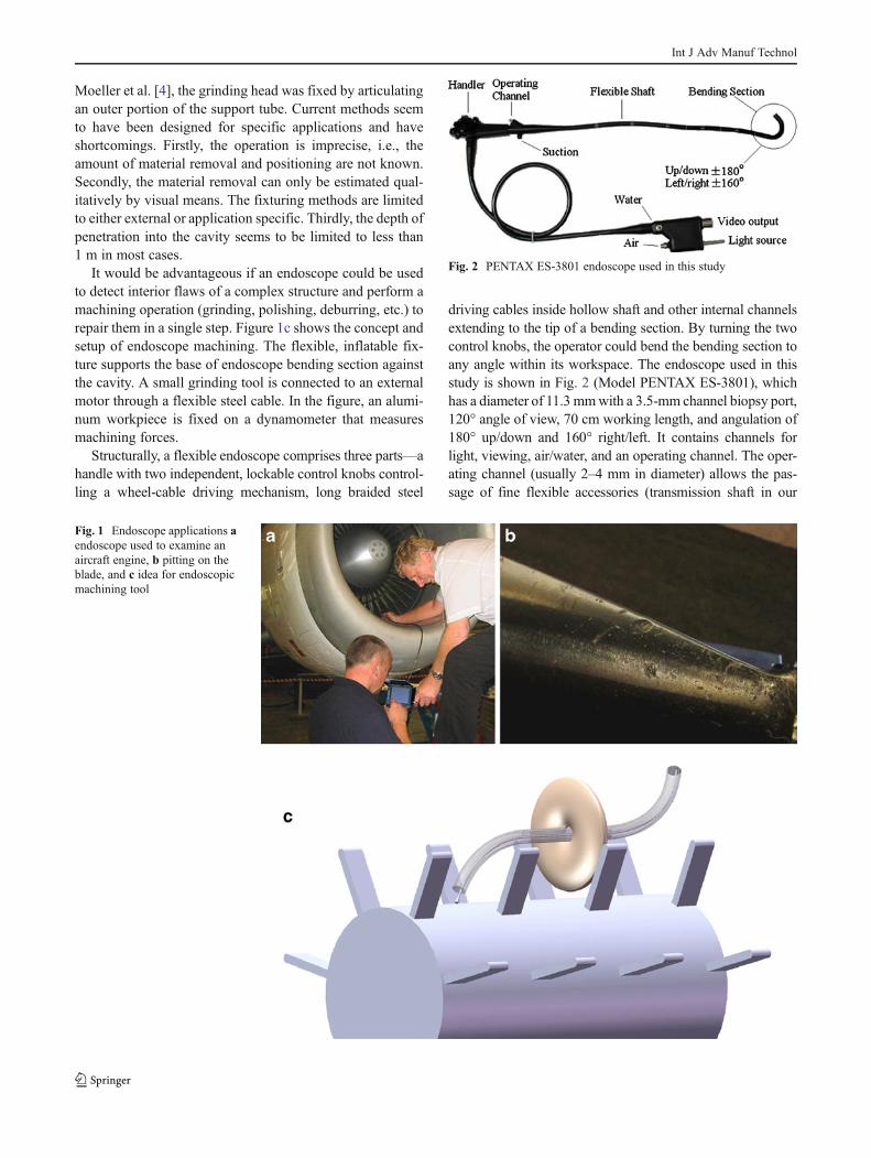
driving cables inside hollow shaft and other internal channelsextending to the tip of a bending section. By turning the twocontrol knobs, the operator could bend the bending section toany angle within its workspace. The endoscope used in thisstudy is shown in Fig. 2 (Model PENTAX ES-3801), whichhas a diameter of 11.3 mmwith a 3.5-mm channel biopsy port,120° angle of view, 70 cm working length, and angulation of180° up/down and 160° right/left. It contains channels forlight, viewing, air/water, and an operating channel. The oper-ating channel (usually 2–4 mm in diameter) allows the pas-sage of fine flexible accessories (transmission shaft in our

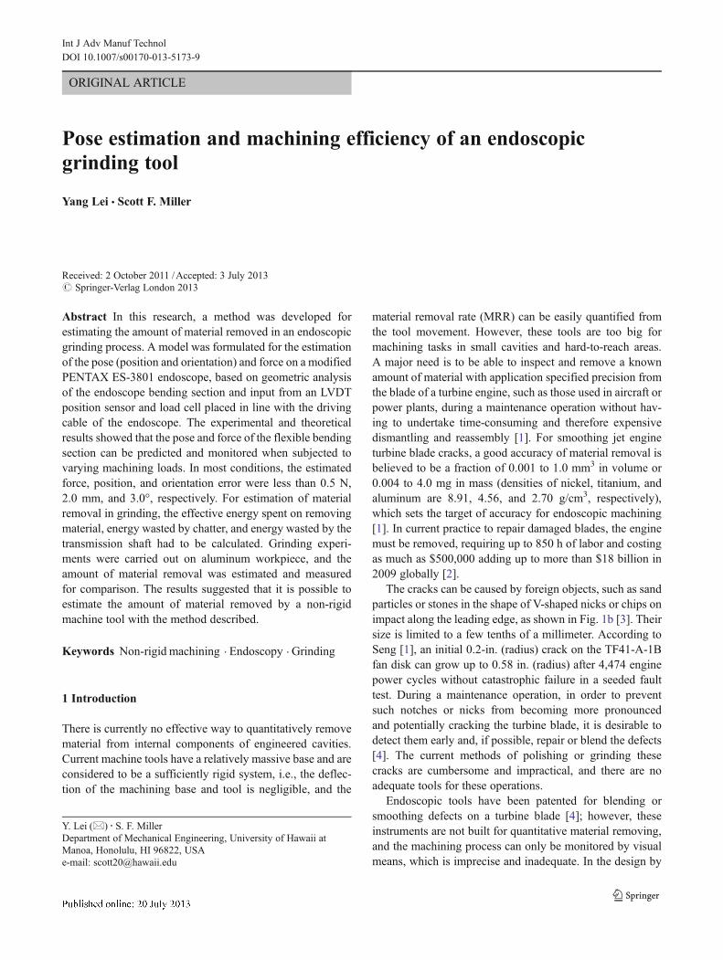
Fig. 1 Endoscope applications aendoscope used to examine anaircraft engine, b pitting on theblade, and c idea for endoscopicmachining tool

Fig. 2 PENTAX ES-3801 endoscope used in this study

Int J Adv Manuf Technol

experiments) from a port on the endoscope control headthrough the shaft and into the field of view.

Ikuta et al. [5] designed and developed a wire-driven 9degree-of-freedom manipulator with 10 mm diameter forminimally invasive surgery called “Hyper Finger.” A specialmechanism by Hirose and Chu [6] was used to address thedrive wire elongation issue. However, force, torque, and loadcapacity of this manipulator were not measured but onlyqualitatively described as “enough.” Hirose and Fukushima[7] introduced a string-driven and snake-like robotic designparadigm for search and rescue tasks. Bionic structures suchas snake and spirochete were used in robotic locomotiondesign. Degani et al. [8] developed a minimally invasivesurgical robot using on a novel two-concentric snakes mech-anism. With a 12 mm in outer diameter and 300 mm in totallength snake-like body, this robot is able to withstand 1 to5 N loads depending on the direction of the load and config-uration of the robot. Mosse et al. [9] invented a device formeasuring the force and torque exerted on the shaft of anendoscope. In this case, the doctor could be aware of thethrust force and reduce the risk of perforating the organduring colonoscopy. Munnae et al. [10] modeled the articu-lated section of a planar cable-driven endoscope as a serialrobot. These studies set the ground work for the currentresearch, but the method for force and pose estimation hasnot been addressed in the literature, and becomes a majorgoal of this research.

The flexibility of long arms has been studied in roboticmachining and control of manipulators. Railbert and Craig[11] described a hybrid technique where force and torqueinformation were combined with positional data for controlof robotic manipulators. Akbari and Higuchi [12] use exter-nal cutting force data to adjust the tool to the workpiecesurface in a grinding operation by a six-axis articulatedrobot. Matsuoka et al. [13] studied the effect of the flexibilityof an articulated robot on an end milling operation. Yu et al.[14] established the rigid and flexible dynamic equations fora polishing machine tool. In this study, the influence offlexibility of each leg on the position of the moving platformwas calculated. Plosa and Wojciech [15] presented mathe-matical and finite element models of beam-like links withbending and torsional flexibility. Zhang et al. [16] presentedthe critical issues and methodologies to improve roboticmachining performance with flexible industrial robots. Theydeveloped a stiffness model and real-time deformation com-pensation was developed to control MRR. After the com-pensation, the surface error of machining a foundry cylinderhead was improved from 0.9 to 0.3 mm. Lipkin and Munnae[17] studied the geometry and kinematic control of an endo-scope using robotics approach. However, none of the methodsin these studies are adequate for precise material removal indifficult-to-reach internal cavities. Current industrial robotsare still too rigid and too big to carry on machining tasks in

narrow cavities where an endoscope could fit. An endoscopictool with precise machining capability is needed, and is thetopic of this paper.

The ultimate goal of this research is the estimation andcontrol of material removal by an endoscopic machiningtool. It was found from initial investigation that the grindingposition and angle of the bending section are critical for themachining condition and material removal estimation. More-over, the position and orientation (pose) and force are inex-tricably coupled in this system. The repeatability and accu-racy of the model were validated by endoscopic materialremoval experiments. Section 2 presents the experimentalsetup for the instrumented endoscope and verification ofpose and force. Sensors were installed onto the endoscope,and a geometric model was built to study the kinetic charac-teristics of the bending section. In Section 3, the static andenergy-based MRR models are described. In the grindingoperation, the endoscopic bending section guided and sup-ported the grinding tool, and the pose of the flexible toolvaried with the applied machining force. The MRR of theendoscopic grinding experiment was estimated by the modeland measured by the difference in mass of the workpiece.Sections 4 and 5 present the setup and results, respectively,for the experimental validation.

1.1 Setup of endoscopic machining experiment

Pose and force of the bending section were measured in realtime in the experiments. The following sections describe thecoordinates for these measurements and the setup of thegrinding experiment for validation of the theoretical model.

1.2 Setup of pose and force measurement

Figure 3 shows the setup with the endoscope which waspartially disassembled and instrumented with a LVDT dis-placement sensor (model Macro Sensors SE750-2000) and aload cell (model Delta Metrics XLUS88). The outer coveringof the endoscope was removed for full access to the drivingcables and bending section. The control handle and the baseof the bending section were rigidly fixed on metal brackets.In this study, only 2D planar movement was considered forproof of concept without any loss of generality. In Fig. 3, theposition of the tip of endoscope (point E) is measured inreference frame {O}. The origin of {O} is coincident withthe fixed base (point B) of bending section.

The displacement and force measurements were used toestimate the pose of the bending section in the modeling inSection 3. Since the tip of the bending section was driven bythe control knob through four steel cables that moveup/down and left/right, the pose and forces of endoscopetip with respect to the base were only a function of thedisplacement and tensile force of the driven cables.


1.3 Visual pose measurement

The pose had to be externally measured by a camera systemfor validation of the model estimation of pose. The 2Dmeasured pose of the tip was independently acquired in realtime using a computer vision approach called object trackingin which markers were attached at crucial points on theendoscope and tracked with customized computer software[18, 19]. The steps in the true position acquisition are asfollows:

1. A camera was placed above and carefully aligned withthe bending sections work plane to get the top view ofthe whole 2D planar work space of the tip, as shown inFig. 3a.

2. Four red markers were attached to the base (B), the tip (Hand E) of bending section and another reference point(R), as shown in Fig. 3b.

3. In MATLAB, input video frames were converted to Red-Green-Blue color space from original YUY2 color spaceand then passed through a color filter to extract all redcolor objects.

4. An object tracking tool called Blob Analysis was appliedto determine the pixel location and centroid of all blobsin video.

5. Position and orientation angle were calculated from thepixel location and centroid.

Figure 3 also shows trigonometric calculation for mea-sured pose from pixel positions. The measured positionof the tip of the bending section, point E, was calculatedusing the pixel values of E and calibrated to the mea-sured distance between base B and reference point R,which was 145.2 mm. Although the camera was careful-ly aligned with the work plane of endoscope, there wasinevitable error in optical channel due to camera deploy-ment, video resolution, lenses distortion, and perspectivedistortion. However, the average error was less than1 mm of measured position acquisition, the resolutionof orientation angle was 0.1°, and the average error wasless than 1°.

1.4 Endoscopic grinding experimental setup

Figure 4 shows the setup of the endoscopic grinding exper-iment for validation of the calculated mass of material re-moved in endoscopic grinding from the MRR model. Theworkpiece is fixed on top of the dynamometer (model Kistler9272). The frictional grinding force and normal grindingforce measured by the dynamometer were used only forcalibration. The endoscope bending section can bend freelyin horizontal workspace but is restricted vertically. The baseof the bending section is fixed between two metal brackets.The workpieces were cut from AISI 6061-T651 aluminumbar, and each piece was approximately 74–76 g. The initialbending angle was 90° and grinding angle was set to zero,which means the grind stone was in full contact with thesurface of the workpiece. For each grinding test, the motorwas set to 5,000 rpm (83.3 Hz).

During the test, the horizontal control knob was turnedto bend the bending section and create the force betweenthe grinding tool and workpiece. The turning force wasquickly increased to a preset level, and the control knobwas locked during grinding. After 30 s of grinding, thecontrol knob was unlocked, and the grinding stone wasremoved. Before and after grinding, each workpiece wasweighed on a Mettler Toledo XP504 precision scale with

Fig. 3 Instrumented endoscopebending section a experimentalsetup with LVDT a load cell andb object tracking to measure thepose

Fig. 4 Setup of 2D endoscopic grinding experiment for MRR modelvalidation


0.1 mg resolution (readability) for measurement of theamount of mass removed.

The model was semi-empirical. Nine workpieces wereground in the first experiment, and the results were used tocalibrate the parameters in the MRR prediction model. An-other two groups of endoscopic grinding experiments wereperformed to validate the repeatability of the model.

2 Theoretical model of endoscopic machining

The pose and force are coupled in the models, i.e., anyexternal force applied to the tip of the bending section resultsin a change in pose. When the driving cables are tensionedby the control knob to bend the bending section, the positionand tension in the driving cables can be measured andmapped to the pose. If an external force is applied to the tipof the bending section, it deflects under the force and its posechanges, which can then be estimated by the increased ten-sion in the driving cables. This is the basis for the modelingin this research.

Initially for simplicity, the pose model was formulatedwithout considering external force. Then, external forcewas added for a more comprehensive model. Figure 5shows the work flow of pose estimation and force predic-tion. First, the LVDT sensor and load cell were carefullycalibrated and compensated for nonlinearity. Second, areal-time readout δ, which is displacement measured bythe LVDT sensor, was used to calculate the pose for freemovement of the endoscope controlled by the drivingcables without an external force. Then, the endoscopewas studied with application of external force. The calcu-lated values from the Geometric Model plus the forcemeasured by the load cell were used to estimate the poseand external force.

2.1 Modeling the pose in free movement

The first step was to calculate the pose for the tip of theendoscope in the simple case of control by the knob withoutexternal force. There is one input, δ, and three outputs, θfree,Yfree, and Xfree which are the angle, Yposition, and X positionof the tip of the bending section, respectively. The geometricmodel comprises three governing equations as shown inEqs. 1–3:

θfree ¼ δRring

ð1Þ

Y free ¼ 2Rsinθfree2

� �sin

π2−θfree2

� �ð2Þ

X free ¼ 2Rsinθfree2

� �cos

π2−θfree2

� �ð3Þ

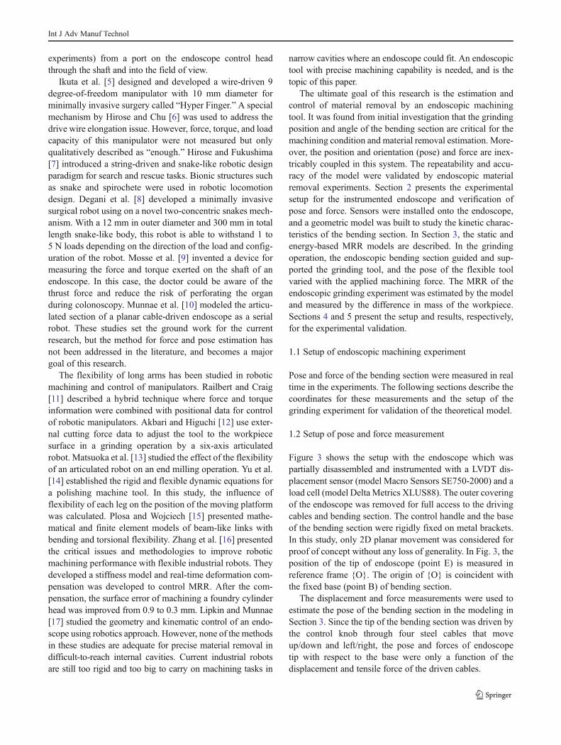
where Rring is the radius of each link of the bending section(5.77 mm) and R is radius of the arc formed by principal axis,which is the distance between points B and E in Fig. 6. Inunforced condition, it is assumed that the principal axis ofbending section will always be an arc on a circle, as shown inFig. 6, with a constant length, L. The accuracy of the geo-metric model was evaluated and is given in Section 5.

The tension in the driving cable was not zero even withoutexternal force because of the biopsy tube (4.5 mm outerdiameter, 0.5 mm wall thickness) that held the transmissionshaft for machining. This intrinsic force was found, as shownin Fig. 7 as the relationship between the driving cable tensileforce measured by the load cell, Fcell, and δ.

2.2 Force prediction model: pose estimation with externalforced

The bending section was modeled with equal length links foraccurate prediction of the pose under forced boundary con-ditions. Then, the tension in the driving cable was character-ized and calibrated to the external force. The forced response

Fig. 5 Flowchart of coupled pose and force model


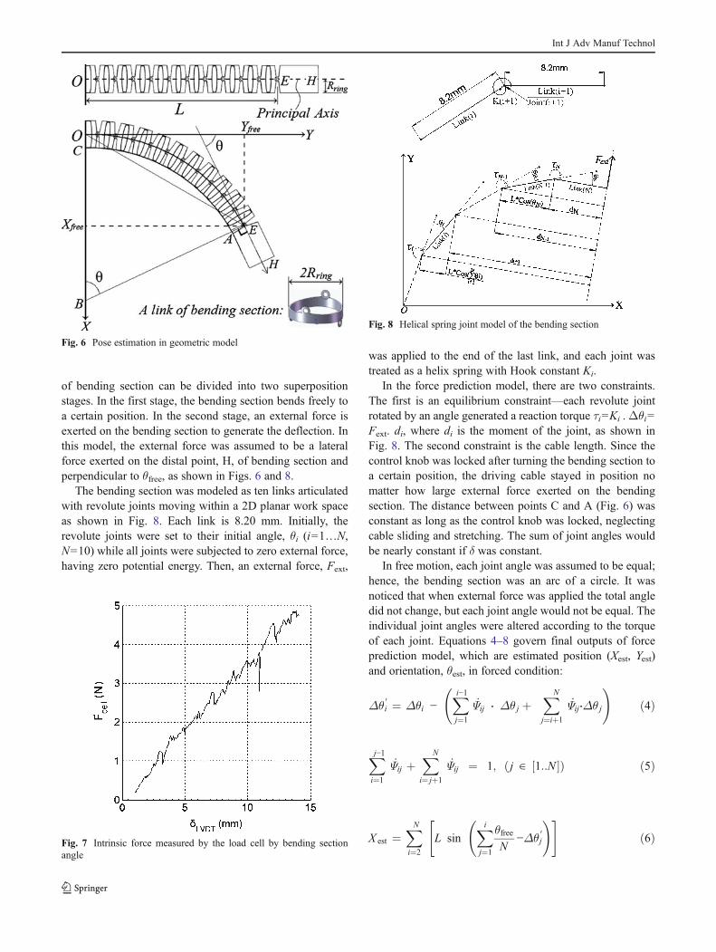
of bending section can be divided into two superpositionstages. In the first stage, the bending section bends freely toa certain position. In the second stage, an external force isexerted on the bending section to generate the deflection. Inthis model, the external force was assumed to be a lateralforce exerted on the distal point, H, of bending section andperpendicular to θfree, as shown in Figs. 6 and 8.

The bending section was modeled as ten links articulatedwith revolute joints moving within a 2D planar work spaceas shown in Fig. 8. Each link is 8.20 mm. Initially, therevolute joints were set to their initial angle, θi (i=1…N,N=10) while all joints were subjected to zero external force,having zero potential energy. Then, an external force, Fext,

was applied to the end of the last link, and each joint wastreated as a helix spring with Hook constant Ki.

In the force prediction model, there are two constraints.The first is an equilibrium constraint—each revolute jointrotated by an angle generated a reaction torque τi=Ki .Δθi=Fext. di, where di is the moment of the joint, as shown inFig. 8. The second constraint is the cable length. Since thecontrol knob was locked after turning the bending section toa certain position, the driving cable stayed in position nomatter how large external force exerted on the bendingsection. The distance between points C and A (Fig. 6) wasconstant as long as the control knob was locked, neglectingcable sliding and stretching. The sum of joint angles wouldbe nearly constant if δ was constant.

In free motion, each joint angle was assumed to be equal;hence, the bending section was an arc of a circle. It wasnoticed that when external force was applied the total angledid not change, but each joint angle would not be equal. Theindividual joint angles were altered according to the torqueof each joint. Equations 4–8 govern final outputs of forceprediction model, which are estimated position (Xest, Yest)and orientation, θest, in forced condition:

Δθ0i ¼ Δθi −

Xj¼1

i−1

Ψ�ij ⋅ Δθ j þ

Xj¼iþ1

N

Ψ�ij⋅Δθ j

!ð4Þ

Xi¼1

j−1

Ψ�ij þ

Xi¼ jþ1

N

Ψ�ij ¼ 1; j ∈ 1::N½ �ð Þ ð5Þ

X est ¼Xi¼2

N

L sinXj¼1

i θfreeN

−Δθ0j

!" #ð6Þ

Fig. 6 Pose estimation in geometric model

Fig. 7 Intrinsic force measured by the load cell by bending sectionangle

Fig. 8 Helical spring joint model of the bending section


Y est ¼ L þXi¼2

N

LcosXj¼1

i θfreeN

−Δθ0j

!" #ð7Þ

θest ¼ θfree −Xi¼2

N

Δθ0i ð8Þ

where Eq. 4 is calculated for each joint. Note that Ψij

(i, j∈[1..N]; i≠ j) are weight factors controlling the redistri-bution of θ. For the estimated external force, Fest, Fig. 9shows the last two joints of bending section in equilibrium.(Fcell−Fint) is the reaction force on the driving cable. Fint isthe intrinsic force plotted in Fig. 7. In equilibrium torquesgenerated by Fext and reaction force should balance each other:

Fext ≈ Fest ¼ Fcell−0:3531δ þ 0:02672

2:788ð9Þ

2.3 Prediction of material removal by energy input

Once the pose and force could be estimated in an endoscopicgrinding process, the material removal could be predicted bycalculating the effective energy input by the grinding tool.This calculation had three inputs (Fcell, δ, and grinding timeduration, T) and generated one output (mass of materialremoval, M). Song et al. [20] found that due to a variety offactors, such as workpiece shape, contact force, robot veloc-ity, and belt wear, precise control of material removal forfree-formed sufaces (e.g., surface of turbine blades and arti-ficial metal joints) using a robotic belt grinding system canbe very challenging. The author proposed an adaptivemodeling method to off-line plan the control parameters forhigh-quality material removal control of robot grindingsystem. Zhang and Pan [21] proposed a practical MRRcontrol method based on experimental identified dynamicmodel and force and power feedback control, which reducesthe vibration and dramatically increases the productivity ofrobotic machining process.

It is thought that if the specific energy of endoscopicgrinding is known, the mass of material removal can beestimated with reasonable accuracy. The specific energy iscommonly used as an inverse measurement of machiningefficiency [22]. In machining, specific energy is defined as

the ratio of machining power to MRR. For traditional grind-ing, specific energy can vary from 10 to 100 J/mm3 for highfeed rate grinding to finish grinding or for soft to very hardsurfaces [22]. Geometric criterion (i.e., cubic millimeters) istypical for calculation of specific energy; however, in taskslike crack smoothing, the geometric approach may not besuitable because the crack may have complicated geometricshape. It is more convenient to use mass criterion in this studybecause it is easy to decide the amount of material removal byweighing the workpiece before and after grinding.

Etot is the total energy spent on grinding, separated intouseful energy on material removal, Es, and wasted energy ontool chatter, Ec, and power transmission, Et, calculated byEq. 10 [23].

Etot ¼ Es þ Ec þ Et

¼ μ δ; Fcellð Þ Fest δ; Fcellð Þ ωTπD ð10Þ

where μ is the ratio of tangential grinding force to normalforce and is dependent on grinding parameters such as grind-ing angle, wheel grain size, wheel wear, workpiece material,Fig. 9 External force balance in equilibrium state

Fig. 10 Effect of chatter on endoscopic grinding


etc., ω is the rotational speed of grinding tool (Hertz), and Dis the tool head diameter. Both μ and Fest were functions of δand Fcell. The expression for μ is given in Table 3. It wasassumed the change of grinding parameters was small

enough to be neglected and, therefore, μ was constant for abatch of grinding tasks.

Equation 11 maps Es to material removal, M, through acoefficient, κ:

M ¼ κ Etot−Ec−Etð Þ ¼ κTω μ δ; Fcellð ÞFext δ; Fcellð ÞπD−Z−θ

θ

PB θð Þdθ−E f

24

35 1−Pcell½ �

8<:

9=; ð11Þ

where PB is the coefficient for the power wasted by bendingthe transmission cable, Ef is the energy wasted by frictionbetween the transmission cable and the endoscope tool chan-nel, and Pcell is the percentage of wasted chatter energy to totalenergy and was a function of the power spectrum of thegrinding energy. Et is the energy wasted on bending the powertransmission cable back and forth in every turn and the contactfriction between the cable and the endoscope tool channel:

2

Z0

θ

PB θð Þdθ0@

1A; PB θð Þ ¼

Xi¼1

n

αi θ−βið Þi ð12Þ

The angle θ was estimated by Eqs. 4 and 8, and thebending power coefficients αi and βiwere calibrated throughexperiments.

2.4 Analysis of machining efficiency

The percentage of energy wasted by chatter had to be estimat-ed in the model for an accurate correlation between the energyand mass removed. Zhang et al. [16] proposed a stiffnessmodeling method to real-time compensate manipulator’s de-formation in order to achieve higher productivity and better

surface accuracy. Pan et al. [24] proposed mode-couplingchatter theory to analyze and suppress chatter in robotic ma-chining process. Matsuoka et al. [13] proposed a more accu-rate flexible end milling process by using small diameter endmilling tool head and high speed spindle.

A relationship was determined between the energy wastedby chatter and the power spectrum of Fcell. Figure 10a shows

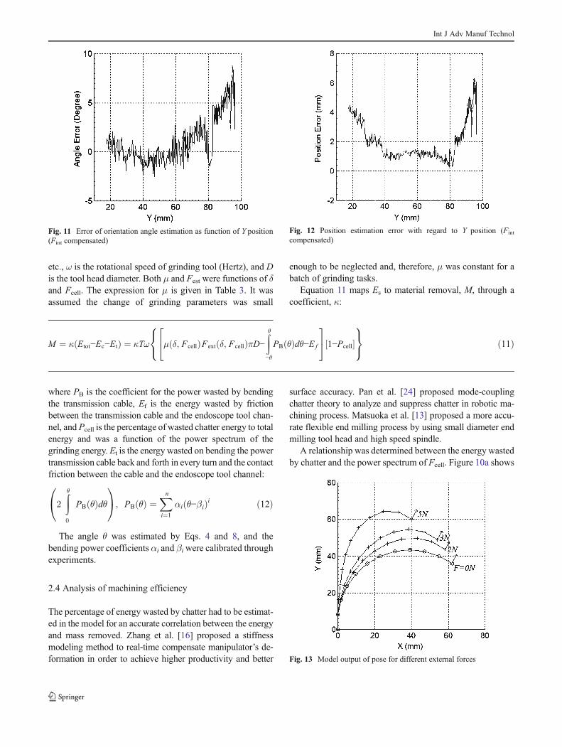
Fig. 11 Error of orientation angle estimation as function of Y position(Fint compensated)

Fig. 12 Position estimation error with regard to Y position (Fint

compensated)

Fig. 13 Model output of pose for different external forces


the difference in surface finish with and without chatter foraluminum samples after 30 s of grinding. The ground texturewithout chatter can be seen as several parallel grindinggrooves, while that with chatter appears to be numerousrandom strokes imprinted on workpiece surface. Figure 10bshows the corresponding Fcell power spectrum of grinding.Most of the grinding energy is concentrated at the first peak ingrinding without chatter, which corresponds to the fundamen-tal frequency of rotary grinding tool. The second and higherorder harmonic peaks are observable in grinding with chatter.

Equation 13 was created to separate the energy wasted bychatter from grinding energy in the model using load cellpower spectrum. P1 is the power of the first harmonic peak.The ith peak has a central frequency located at fi and thebreadth of that peak is from fi

− to fi+ in frequency domain.

For grinding without chatter, 99 % of its first peak power isin the range of 35 to 60 Hz.

Ec ¼ Etot−Etð ÞPcell; Pcell ¼ 1−

Zf −1

tþ1

λiPi fð Þdf

Xi¼1

N Zf −1

fþ1

λiPi fð Þdf

0BBBBBBBBBB@

1CCCCCCCCCCA

ð13Þ

Since the tensile force measured by the load cell wasindirectly related to the grinding energy and the driving cablewas a nonlinear component, the Pcell was not directly used inthe calculation of wasted energy by chatter. Therefore, a setof empirical power compensating coefficients (λ1 to λN)were applied on Pi (i∈[1..N]). Experiments were conductedto acquire empirical data to specify the force ratio function μ,power compensating coefficients λ1 to λN, and the bendingpower coefficient αi and βi, and these will be presented in theresults.

3 Experiment results and model evaluation

3.1 Model results for pose and external force

Figures 11 and 12 show the orientation angle error andposition error for Xest, Yest, and θest calculated by Eqs. 6–8.These results are achieved by simply setting all weightfactors Ψij to a constant 1

N−1 . By compensating bendingsection deflection caused by internal driving force, the esti-mation accuracy is improved by at least 100 % for allpositions. In most conditions, the estimated force, position,and orientation error were less than 0.5 N, 2.0 mm, and 3.0°,respectively. For the endoscope used in this study, theseerrors are reasonable, and the method was proven valid.

Figure 13 shows the results for pose estimation calculatedby Eqs. 4–8 for four external forces. It gives an intuitive viewon how the force prediction model works. The joint numberwas set to J=10, and the initial angle of bending section wasset as θfree=120° in this example. Hook constant, Ki, of eachjoint was set to 10. The weight factor was setΨij=1/(N−1) (i,j∈[1..N], i≠ j, N=10) for all ten joints. The external force,Fext, was set to 0, 2, 3, and 5 N, and the simulation wasexecuted to get compensated orientation angle and tip posi-tion. Each marker in Fig. 13 represents a pivot joint wherethe links come together.

The error in the estimated force calculated by Eq. 9 wasevaluated at discrete points under different Fext. Table 1

Table 1 Force prediction error for different position-forcecombinations

Fext (N) θfree=90° 120° 140° 160°

0 −0.537 −0.605 −0.650 −0.361

1 −0.036 −0.457 −0.484 −0.393

2 0.307 −0.222 −0.433 −0.317

3 0.592 0.078 −0.501 −0.445

4 −0.424 −0.150

5 −0.017 −0.246

6 −0.242

Table 2 Position and angle prediction error for different position–forcecombinations

Position error (mm)/angle error (°)

Fext (N) θfree=90° 120° 140° 160°

1 1.2/2.1 1.1/0.8 2.5/3.3 4.1/3.5

2 2.2/0.8 1.7/4.3 3.4/−0.8 3.2/−0.7

3 2.7/5.5 2.5/6.0 4.9/5.5 6.3/5.8

4 6.1/−8.5 5.9/−2.4

5 7.7/−10.4 2.8/−10.2

6 8.9/−15.6

Table 3 Experimentally calibrated model parameters

Bending angle (°) θ (0.6483δ2+12.08δ−0.0597)/0.5766+Fcell (t) dt/1,000

Force ration μ 1.2 cos(θ–.815)

Chatter coefficients λ1 1

λ2 0.9

λ3 20

Transmission coefficients α1 0.08

β1 90

Energy coefficient κ 1.3e−3


shows the difference in measured and estimated force fordifferent position-force combinations. In most conditions,the estimated force error is less than 0.5 N. Note that whenθfree is less than 90°, the bending section cannot withstandmuch external force; hence, the combinations with smallerbending angle were not evaluated. Table 2 shows the error ofposition and orientation calculated by Eqs. 6–8 in differentforced conditions. Note that when external force was lessthan 4 N, the estimation error is low. When external forceexceeds 5 N, the bending section buckles in vertical direc-tion, its principal axis is not in the horizontal plane, andestimation errors increase greatly.

3.2 Comparison between measured and calculated materialremoval

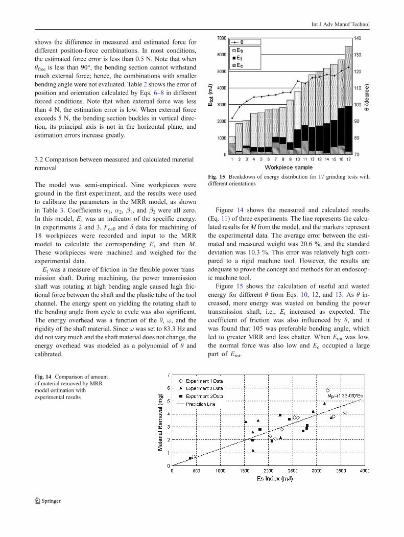
The model was semi-empirical. Nine workpieces wereground in the first experiment, and the results were usedto calibrate the parameters in the MRR model, as shownin Table 3. Coefficients α1, α2, β1, and β2 were all zero.In this model, Es was an indicator of the specific energy.In experiments 2 and 3, Fcell and δ data for machining of18 workpieces were recorded and input to the MRRmodel to calculate the corresponding Es and then M.These workpieces were machined and weighed for theexperimental data.

Et was a measure of friction in the flexible power trans-mission shaft. During machining, the power transmissionshaft was rotating at high bending angle caused high fric-tional force between the shaft and the plastic tube of the toolchannel. The energy spent on yielding the rotating shaft tothe bending angle from cycle to cycle was also significant.The energy overhead was a function of the θ, ω, and therigidity of the shaft material. Since ω was set to 83.3 Hz anddid not vary much and the shaft material does not change, theenergy overhead was modeled as a polynomial of θ andcalibrated.

Figure 14 shows the measured and calculated results(Eq. 11) of three experiments. The line represents the calcu-lated results forM from the model, and the markers representthe experimental data. The average error between the esti-mated and measured weight was 20.6 %, and the standarddeviation was 10.3 %. This error was relatively high com-pared to a rigid machine tool. However, the results areadequate to prove the concept and methods for an endoscop-ic machine tool.

Figure 15 shows the calculation of useful and wastedenergy for different θ from Eqs. 10, 12, and 13. As θ in-creased, more energy was wasted on bending the powertransmission shaft, i.e., Et increased as expected. Thecoefficient of friction was also influenced by θ, and itwas found that 105 was preferable bending angle, whichled to greater MRR and less chatter. When Etot was low,the normal force was also low and Ec occupied a largepart of Etot.

Fig. 15 Breakdown of energy distribution for 17 grinding tests withdifferent orientations

Fig. 14 Comparison of amountof material removed by MRRmodel estimation withexperimental results


4 Conclusions

In this research, the methods for measuring and estimatingthe pose of the bending section of the endoscope and thematerial removal in an endoscopic grinding operation weredeveloped and tested. The major conclusions are:

& It was found that the pose and force on the flexible endo-scopic tool could be reasonably estimated and trackedduring machining operation. In most conditions, the esti-mated force, position, and orientation error were less than0.5 N, 2.0 mm, and 3.0°, respectively.

& The results revealed that when bending angle is small andnormal force is small, chatter will occupy a large percentof grinding energy. When normal force is large and bend-ing angle is large, the power transmission overhead willbecome the dominant factor of wasted energy.

& It was found that the amount of material removed can bepredicted in a flexible, endoscopic machining operation.The material removal prediction model showed that in2D configuration, the average prediction error is 20.6 %for the 27 samples tested. This is a significant error, butthe results suggested that the methods developed in thisresearch are feasible for predicting MRR for a flexible,endoscopic machining task. The error in the predictionscould be reduced by improving the accuracy and precisionof the tracking equipment, sensors, and endoscopicbending section structure.

References

1. Silvia S (2004) Turbine engine fan disk crack detection test.Weapons Survivability Laboratory Final Report DOT/FAA/AR-04/28, September 2004

2. Markou C, Cros G, Cioranu A, and Yang E (2011) Airline Main-tenance Cost Executive Commentary. Maintenance Cost TaskForce. http://www.iata.org/whatwedo/workgroups/Documents/MCTF/AMC_ExecComment_FY09.pdf. Accessed 22 Jan 2013

3. Carter TJ (2005) Common failures in gas turbine blades. Eng FailAna 12(2):237–247

4. Moeller D, Moeller HD, Moeller DB (2005) Grinding apparatus forblending defects on turbine blades and associated method of use.US Patent 6:899,593

5. Ikuta K, Hasegawa T, and Daifu S (2003) Hyper redundant miniaturemanipulator “hyper finger” for remote minimally invasive surgery in

deep area. Proc IEEE Int Conf Rob & Aut, Taipei, Taiwan, September2003, 1:1098–1102

6. Hirose S, Chu R (1999) Development of a light weight torquelimiting m-drive actuator for hyper redundant manipulator floatarm. Proc IEEE Int Conf Rob & Aut 2831–2836

7. Hirose S, Fukushima E (2004) Snakes and strings: new roboticcomponents for rescue operations. Int J Rob Res 23(4–5):341–349

8. Degani A, Choset H, Wolf A, Zenati M (2006) Highly articulatedrobotic probe for minimally invasive surgery. Proc IEEE Int Confon Rob & Aut 4167–4172

9. Mosse CA, Mills TN, Bell GD, Swain CP (1998) Device formeasuring the forces exerted on the shaft of an endoscope duringcolonoscopy. Med & Bio Eng & Comp 36:186–190

10. Munnae J, McMurray G, Lipkin H (2010) Static and kinematicanalysis of a planar cable-driven flexible endoscope. Proc ASMEInt Des Eng Tech & Comp Info in Eng Conf 7:65–74, DETC2009(PARTA)

11. Raibert MH, Craig JJ (1981) Hybrid position/force control ofmanipulators. J Dyn Syst Meas & Cont, Trans of ASME 103(2):126–133

12. Akbari AA, Higuchi S (2002) Autonomous tool adjustment inrobotic grinding. J Mater Process Tech 127(2):274–279

13. Matsuoka S, Shimizu K, Yamazaki N, Oki Y (1999) High speedend milling of an articulated robot and its characteristics. J MaterProcess Tech 95(1–3):83–89

14. Yu M, Zhao J, Zhang L, Wang Y (2004) Study on the dynamiccharacteristics of a virtual-axis hybrid polishing machine tool byflexible multibody dynamics. Proc Inst Mech Eng, Part B: J EngManuf 218(9):1067–1076

15. Plosa J, Wojciech S (2000) Dynamics of systems with changingconfiguration and with flexible beam-like links. Mechan & MachTheor 35(11):1515–1534

16. Zhang H, Wang J, Zhang G, Zhongxue G (2005) Machining withflexible manipulator: toward improving robotic machining perfor-mance. IEEE/ASME Int Conf on Adv Int Mech, AIM 2:1127–1132

17. Lipkin H, Munnae J (2007) Endoscope geometrical analysis andkinematic control. Proc ASME Int Des Eng Tech Conf & Comp &Inf in Eng Conf 8:231–238

18. Steger C, Ulrich M., and Wiedemann C (2008) Machine Visionalgorithms and applications 1st ed. Wiley, Darmstadt

19. Shapiro LG and Stockman GC (2001) Computer vision. PrenticeHall, Upper Saddle River

20. Song Y, Liang W, and Yang Y (2011) A method for grindingremoval control of a robot belt grinding system. J Int Manuf 1–11doi: 10.1007/s10845-011-0508-6

21. Zhang H and Pan Z (2011) Robotic machining: material removalrate control with a flexible manipulator. IEEE InternationalConference on Robotics, Automation and Mechatronics, RAM,September 2008 4690881:30–35

22. Marinescu ID, RoweWB, Dimitrov B, Inaski I (2004) Tribology ofabrasive machining process, 1st ed. William Andrew Inc, Norwich

23. Kannappan S, Malkin S (1972) Effects of grain size and operatingparameters on the mechanics of grinding. J Eng Ind Trans ASME94(3):833–842

24. Pan Z, Zhang H, Zhu Z, Wang J (2006) Chatter analysis of roboticmachining process. J Mater Process Tech 173(3):301–309


http://www.iata.org/whatwedo/workgroups/Documents/MCTF/AMC_ExecComment_FY09.pdf

http://www.iata.org/whatwedo/workgroups/Documents/MCTF/AMC_ExecComment_FY09.pdf

http://dx.doi.org/10.1007/20s10845-011-0508-6