portugal in the euro the roots of stagnation
TRANSCRIPT

PORTUGAL IN THE EURO: THE ROOTS OF STAGNATION
José Manuel de Sá Carneiro
Doctoral Thesis in Economics
Supervisors:
Álvaro Pinto Coelho de Aguiar
Luís Francisco Aguiar-Conraria
September 2019

ii
Para a Zé e os nossos netos, Matilda e António

iii
Biography
José Sá Carneiro was born on 7 April 1955, in Angola. He married Maria José Carneiro.
They are parents of four and grandparents of two. He started the undergraduate degree in
Economics at the University of Luanda, in 1972, and completed it at FEP, in 1977. He
spent most of his professional life working on managerial and investment management
activities across multiple sectors and companies (Amorim Group, Banco Privado
Português, and Fundação Luso-Americana para o Desenvolvimento). Currently, he
teaches Political Economy and Microeconomics at the Universidade Portucalense in
Porto. He received a master’s degree in Economics from FEP in 2002. The dissertation,
supervised by Professor Mário Rui Silva, was entitled “Os Factores não Económicos do
Desenvolvimento Económico: um Teste à Hipótese de Weber” (“The Non-economic
Determinants of Economic Development: A Test to the Max Weber’s Hypothesis”).
Occasionally, he published opinion articles in the Portuguese press (Expresso) and
collaborated as an economic commentator on TV (SIC Notícias).

iv
Acknowledgments
The School of Economics and Management of the University of Porto (FEP) has provided
the right incentives to pursue my interests in economics. Those incentives stem from the
high standards of the education delivered and are grounded in the qualifications of the
FEP's teachers and the exceptional contribution of the invited professors during the PhD
program.
For sure, those standards have been built after decades of hard work. Therefore, my
first expression of gratitude goes to Professor José da Silva Costa. He was the Director of
FEP when I undertook the Master’s degree in Economics in 1997-2002, and an
unforgettable teacher of regional economics. (I never forgot his lecture on von Thünen
and the discussion of the Samuelsson’s paper on the spatial equilibrium model).
The next word is for Professor António Brandão, the Director of the PhD program. He
taught Industrial Economics when I took the Master’s degree (I still remember his so
brilliant introductory lecture on market structures) and Microeconomics in the PhD
coursework.
I move now to the thesis work. I was fortunate to face truly critical examiners along
the successive stages of research and writing. Namely, Professors Anabela Carneiro and
Manuel Mota Freitas at the Thesis Project Defense Examination; and Professors João
Loureiro and again Manuel Mota Freitas at the Interim Defense. Their careful and strict
evaluation of the work in progress allowed me to attain – as now I expect to have reached
– the requirements of academic work.
My interest in human interactions and its connection with the advance of the common
good – is not that the purpose of economics as we have seen in Alfred Marshall? – led me
to other fields in social sciences. Namely, to sociology, for which I have had the support
of a special teacher, my old colleague from the Faculty of Economics of Luanda (Angola),
Rui Pena Pires. He is a distinguished professor of sociology in ISCTE, and I owe this old
friend the introduction to the work of Anthony Giddens. The insight for the concept of
"institutional endowment" presented in the second Essay of this thesis came from the
Giddens approach to Modernity and, more specifically, the property of “reflexivity” that
characterizes modern societies.
Last but not least, my gratitude to the supervisors Professors Álvaro Aguiar and Luís
Aguiar-Conraria. Without their guidance, I would have material for a thesis, but certainly

v
not a thesis. I further acknowledge their generosity for having accepted the role of
supervisors promptly, considering that the probability of someone with other professional
occupations to complete a PhD thesis is not very high.
One final word to my younger colleagues in the PhD coursework who were very
generous for giving up their time in helping me to deal with the "new technologies"
(MATLAB, EndNote...). Namely, and without disregarding all the others, José Pedro
Fique, Ricardo Biscaia, Fernando Coelho, Vera Rocha, Rita Bastião and José Gaspar.
vi
Abstract
An intriguing question motivated this thesis: Why did the Portuguese economy stagnate
after the euro adoption? Economic growth is expected when moving towards more
advanced institutions. Furthermore, a stable monetary policy is not supposed to harm
resources development and allocation.
I tackled this problem with a Marshallian flavor, starting by identifying what had
changed, and after that seeking how might it have hindered economic growth. I found
empirical evidence on a regime change in relative prices. Namely, the price of future to
present consumption (i.e., the real interest rate) and the nominal exchange rate. By
accessing the euro area, Portugal moved up in financial integration. A demand shock and
overvaluation, driven by a credit boom, are typical outcomes of a shift in financial
integration. Although, this time, the capital inflows were drawn from a “common pool”
of savings, and the compression of the interest rates differentials turned structural.
Overvaluation impacting institutions that are biased against larger and more efficient
enterprises not only hampers economic growth at the “frontier” but leads to misallocation
of resources, both between sectors and within-industry. When the institutional framework
is less endowed with the reflexivity property – a concept borrowed from the field of
sociology – the persistent overvaluation episode articulates with hard to change
institutional frictions. That mechanism solves the problem of the long-lasting impact of a
regime change in relative prices on economic growth.
The thesis is composed of three essays. The first is more specific to the stagnation of
the Portuguese economy. The second addresses the euro area experiment as a whole, the
cleavages between the Core and the Periphery, and the productivity slowdown observed
for selected Peripheral countries (Italy, Portugal and Spain). Finally, the third resumes
the analysis of the euro experiment, but now in the short-run time frame, by entertaining
oil shocks on the output and inflation.
vii
Resumo
Uma questão intrigante motivou esta tese: Por que estagnou a economia portuguesa após
a adoção do euro? O crescimento económico é esperado quando um país se move em
direção a um quadro institucional mais evoluído. Para além disso, não é suposto que a
prevalência de uma política monetária seja adversa ao desenvolvimento e alocação dos
recursos.
É com um “sabor” Marshalliano que eu abordo este problema, começando por
identificar o que mudou, e em seguida explorando a forma pela qual as alterações
observadas possam ter afetado o crescimento económico. Encontrei evidência empírica
sobre uma mudança no regime dos preços relativos. Nomeadamente, no preço do
consumo presente em termos do consumo futuro (i.e., a taxa real de juro) e na taxa
nominal de câmbio. Com a integração na área do euro, Portugal subiu no nível de
integração financeira. Um choque da procura e um episódio de sobrevalorização,
determinados por um boom de crédito, são consequências típicas de um salto em
integração financeira. Contudo, desta vez, o afluxo de capitais teve origem em uma
common pool de poupanças, e assim a compressão do diferencial nas taxas de juro tornou-
se estrutural.
Uma sobrevalorização, impactando em instituições enviesadas contra as grandes e
mais eficientes empresas, não apenas atinge o crescimento económico na “fronteira”
como ainda conduz à má-alocação de recursos, entre setores e intra-sectorial. Quando um
quadro institucional é menos dotado na propriedade da reflexividade — um conceito
tomado da sociologia — então um episódio de sobrevalorização articula-se com “fricções
institucionais” resistentes à mudança. Este mecanismo explica os efeitos de longo prazo
de uma mudança no regime de preços relativos sobre o crescimento económico.
A presente tese compõe-se de três ensaios. O primeiro é mais específico sobre a
estagnação da economia portuguesa. O segundo aborda a experiência da área do euro no
seu conjunto, incluindo as clivagens entre o Core e a Periferia, e o abrandamento da
produtividade observado em três países selecionados (Itália, Portugal e Espanha).
Finalmente, o terceiro retoma a análise da experiência do erro, porém desta feita no
horizonte de curto prazo, utilizando choques do petróleo sobre o produto (PIB) e a
inflação.

viii
Contents
INTRODUCTION 1
ESSAY NO. 1: PORTUGAL IN THE EURO: THE ROOTS OF STAGNATION 7
1. INTRODUCTION 8
2. BASIC FACTS AND AN HISTORICAL ACCOUNT 11
2.1 The “Carnation Revolution” 12
2.2 The “EEC Experiment” 15
2.3 The “Euro Experiment” 16
2.3.1 Relative Prices 17
2.3.2 The Impact on Productivity 21
3. THE EMPIRICAL MODEL 23
3.1 Methodology 23
3.2 The Model Specification 24
3.3 Data, Sample and Computation Program 27
3.4 Testing for Unit Roots and Weak Exogeneity 29
3.5 Specification Tests and Break Dates 30
4. EMPIRICAL RESULTS 31
4.1 Contemporaneous Effects 31
4.2 Impulse Response Analysis 34
4.3 Analysis of Long Run 38
4.4 Robustness 44
5. CONCLUSION 45
APPENDIX A 47
APPENDIX B 54
APPENDIX C 70
REFERENCES 77
ESSAY NO. 2: PUZZLING AROUND THE EURO EXPERIMENT 81
1. INTRODUCTION 82
2. IS THE EURO AREA AN OCA? 85
3. THE EURO AREA FAULT LINES 89
3.1 Current Account Asymmetries and Competitiveness Developments 91
3.2 The Role of the Nominal Exchange Rate 94
3.3 The Technological Shock 96

ix
4. THE INSTITUTIONAL ENDOWMENT 101
4.1 The Historical Legacy 101
4.2 Labor Market Institutions and the Institutional Endowment 104
5. THE MISALLOCATION STORY REVISITED 110
6. CONCLUSIONS 114
REFERENCES 115
ESSAY NO. 3: DYNAMICAL ANALYSIS OF THE EURO AREA USING OIL SHOCKS
– A GVAR APPROACH 121
1. INTRODUCTION 122
2. BASIC FACTS 125
2.1 Oil Shocks Episodes 125
2.2 Oil Demand Shocks and Economic Structures 128
3. THE EMPIRICAL MODEL 129
3.1 The Model Specification 131
3.2 The Oil Prices as Dominant Variable 133
3.3 Data, Sample and Observation Windows 134
4. RESULTS AND DISCUSSION 137
4.1 Large/Open Economies 137
4.2 Euro Adopters 141
4.3 Robustness 146
5. CONCLUSION 146
APPENDIX A 148
APPENDIX B 152
REFERENCES 160

x
List of Figures
Essay No. 1
Figure 1. Portuguese Real GDP per Capita, annual Growth Rate Averaged ………… 12
Figure 2. Real Short-term Interest Rate .......................................................................... 17
Figure 3. Unit Labor Costs – HP trend ........................................................................... 18
Figure 4. The Relative Purchasing Power Parity for Portugal and the Output Gap ....... 20
Figure 5. Generalized Impulse Response of a Negative Unit (1 s.e.) Shock to U.S. Real
Equity Prices on Real Output per capita . ............................................................... 34
Figure 6. Generalized Impulse Response of a Positive Unit (1 s.e.) Shock to Oil Prices
on Inflation .............................................................................................................. 35
Figure 7. Generalized Impulse Response of a Positive Unit (1 s.e.) Shock to U.S. Short-
Term Interest Rate on Long-term Interest Rates ................................................... 36
Figure 8. Generalized Impulse Response of a Negative Unit (1 s.e.) Shock to EA-Core
Real Equity Prices on the Real Exchange Rate. ..................................................... 37
Figure 9. Generalized Impulse Response of a Positive Unit (1 s.e.) Shock to U.S. Real
Output per Capita on Real Output per Capita. ........................................................ 38
Figure 10. Persistence Profile of the Effect of System-Wide Shocks to the
Cointegrating Relations. ......................................................................................... 39
Figure 11. Persistence Profile of the Effect of System-Wide Shocks to the Cointegrating
Relations. ................................................................................................................ 40
Figure A. 1. Annual Real GDP per Capita Growth Rate (HP Trend) 53
Essay No. 2
Figure 1. Current Account (in % of GDP): .................................................................... 90
Figure 2. Unit Labor Costs ............................................................................................. 92
Figure 3. The Euro-Dollar Nominal Exchange Rate Trend. ........................................... 95
Figure 4. Total Factor Productivity: Peripheral Countries and Germany. ..................... 97
Figure 5. Real GDP Growth Rate: Peripheral Countries and Euro Area Average. ....... 98
Figure 6. Financial Development Index (FD Index). ...................................................... 99
Figure 7. Unemployment: Germany, Euro Area, United Kingdom and USA. ............ 104
Figure 8. Germany: Unemployment Rate and Unit Labor Costs Trends. ................... 107
Figure 9. Unemployment Rate and Unit Labor Costs Trends. .................................... 108
Essay No. 3
Figure 1. Oil Price Shocks Episodes ............................................................................. 126
Figure 2. Exports to China ............................................................................................ 128
Figure 3. Estimated Responses of Real Output to an Oil Price Shock. ........................ 136
Figure 4. Estimated Responses of Inflation to an Oil Price Shock. .............................. 138
Figure 5. Estimated Responses of Sort-term Interest Rates to an Oil Price Shock. ..... 140
Figure 6. Estimated Responses of Real Output to an Oil Price Shock. Euro Adopters 142
Figure 7. Estimated Responses of Inflation to an Oil Price Shock. Euro Adopters. .... 144
Figure A. 1. Estimated Responses of Sort-term Interest Rates to an Oil Price Shock. 148
Figure A. 2. Estimated Responses of Real Output to a Negative (1 s.e.) Global Shock to
Real Equity Prices. Euro Adopters. ...................................................................... 149
xi
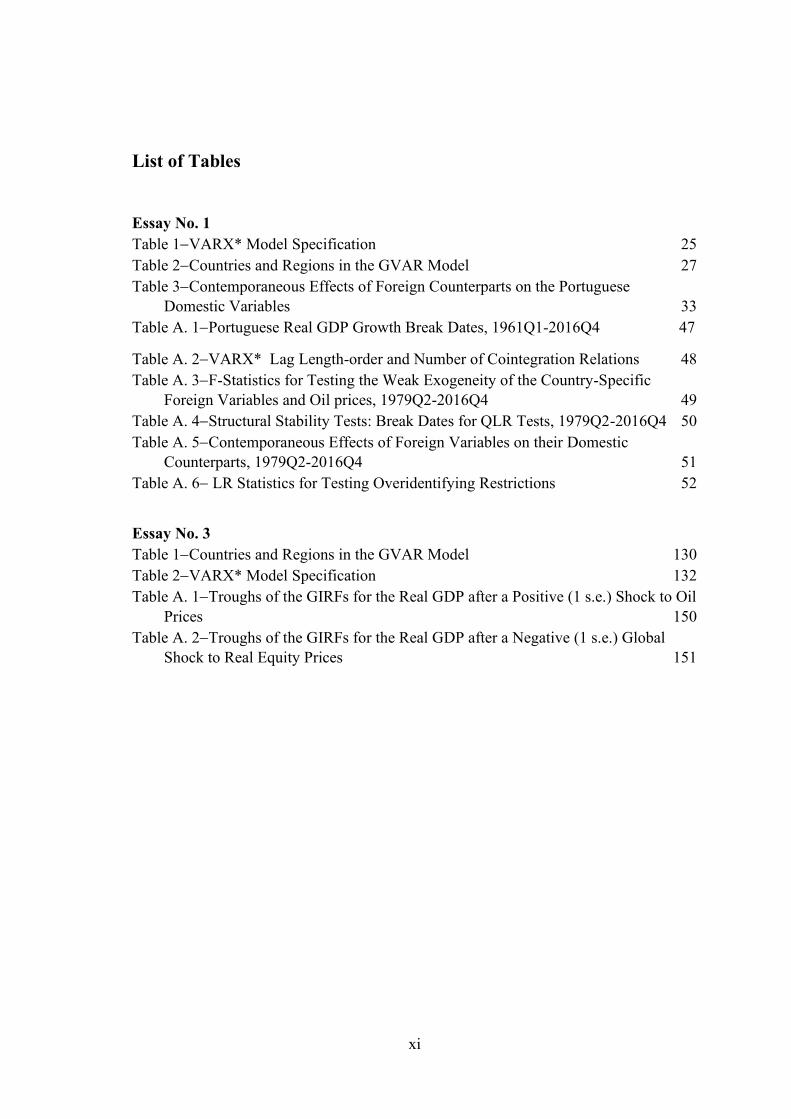
List of Tables
Essay No. 1
Table 1−VARX* Model Specification 25
Table 2−Countries and Regions in the GVAR Model 27
Table 3−Contemporaneous Effects of Foreign Counterparts on the Portuguese
Domestic Variables 33
Table A. 1−Portuguese Real GDP Growth Break Dates, 1961Q1-2016Q4 47
Table A. 2−VARX* Lag Length-order and Number of Cointegration Relations 48
Table A. 3−F-Statistics for Testing the Weak Exogeneity of the Country-Specific
Foreign Variables and Oil prices, 1979Q2-2016Q4 49
Table A. 4−Structural Stability Tests: Break Dates for QLR Tests, 1979Q2-2016Q4 50
Table A. 5−Contemporaneous Effects of Foreign Variables on their Domestic
Counterparts, 1979Q2-2016Q4 51
Table A. 6− LR Statistics for Testing Overidentifying Restrictions 52
Essay No. 3
Table 1−Countries and Regions in the GVAR Model 130
Table 2−VARX* Model Specification 132
Table A. 1−Troughs of the GIRFs for the Real GDP after a Positive (1 s.e.) Shock to Oil
Prices 150
Table A. 2−Troughs of the GIRFs for the Real GDP after a Negative (1 s.e.) Global
Shock to Real Equity Prices 151

1
INTRODUCTION
The Portuguese economy has stagnated for 17 years since the euro adoption, that is
between 1989 and 2016, which is the period under analysis here. Why? This a challenging
question, because we expect less-developed economies to catch up with the frontier,
whenever supported by good institutions. And by accessing the European monetary
union, Portugal moved up into a more advanced institutional setting.
To the best of our knowledge, the main explanations point to (i) competitiveness
impairments (Blanchard 2007) and (ii) resources misallocation, either between-sector
(Reis 2013) or within-industry (Dias et al. 2016). Financial integration led both to an
overvaluation episode underlying the competitiveness issue and a boom of capital inflows
allocated to less efficient entrepreneurs. Financial frictions, related to the lack of capital
deepening, were at the root of the misallocation story of Reis (2013). The more efficient
entrepreneurs, mostly in the tradables sector, were credit constrained. While “firm sized-
contingent” regulations were the possible source of within-industry loss of allocative
efficiency in Dias et al. (2016), by reducing the costs of capital and labor for the smaller
firms.
The thesis presented in the first essay builds on those approaches but argues for a
more comprehensive explanation. Neither macroeconomic factors alone, nor institutional
distortions, are enough to account for the dismal performance of the Portuguese economy.
We must take both and its interaction to find a sound explanation. The bias against larger
and more efficient enterprises was not born with the introduction of the euro. And we
should not be restricted to financial frictions when acknowledging the role of financial
integration. Claiming that more efficient entrepreneurs were credit constrained might
even imply some myopia from the financial system. This thesis argues that a change in
relative prices was the channel through which financial integration guided the resources
to a poor allocation, given some sort of institutional frictions.
I submitted the hypothesis of a regime change in relative prices (i.e., the real interest
rates and the nominal exchange rate) to an econometric evaluation. The global VAR
(GVAR) was the methodology employed. I showed that the referred hypothesis, which
2
implies a shift in the real exchange rate, was subsumable in the relative Purchase Parity
Power (PPP) condition. The relative PPP holds when tested over the period 1979(Q2)-
1998(Q4) but is rejected when the data include the euro time span, that is when the
econometric test is run over 1979(Q2)-2016(Q4).
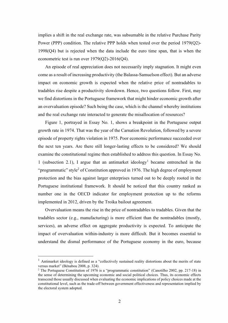
An episode of real appreciation does not necessarily imply stagnation. It might even
come as a result of increasing productivity (the Balassa-Samuelson effect). But an adverse
impact on economic growth is expected when the relative price of nontradables to
tradables rise despite a productivity slowdown. Hence, two questions follow. First, may
we find distortions in the Portuguese framework that might hinder economic growth after
an overvaluation episode? Such being the case, which is the channel whereby institutions
and the real exchange rate interacted to generate the misallocation of resources?
Figure 1, portrayed in Essay No. 1, shows a breakpoint in the Portuguese output
growth rate in 1974. That was the year of the Carnation Revolution, followed by a severe
episode of property rights violation in 1975. Poor economic performance succeeded over
the next ten years. Are there still longer-lasting effects to be considered? We should
examine the constitutional regime then established to address this question. In Essay No.
1 (subsection 2.1), I argue that an antimarket ideology1 became entrenched in the
“programmatic” style2 of Constitution approved in 1976. The high degree of employment
protection and the bias against larger enterprises turned out to be deeply rooted in the
Portuguese institutional framework. It should be noticed that this country ranked as
number one in the OECD indicator for employment protection up to the reforms
implemented in 2012, driven by the Troika bailout agreement.
Overvaluation means the rise in the price of nontradables to tradables. Given that the
tradables sector (e.g., manufacturing) is more efficient than the nontradables (mostly,
services), an adverse effect on aggregate productivity is expected. To anticipate the
impact of overvaluation within-industry is more difficult. But it becomes essential to
understand the dismal performance of the Portuguese economy in the euro, because
1 Antimarket ideology is defined as a “collectively sustained reality distortions about the merits of state
versus market” (Bénabou 2008, p. 324). 2 The Portuguese Constitution of 1976 is a “programmatic constitution” (Canotilho 2002, pp. 217-18) in
the sense of determining the upcoming economic and social political choices. Thus, its economic effects
transcend those usually discussed when evaluating the economic implications of policy choices made at the
constitutional level, such as the trade-off between government effectiveness and representation implied by
the electoral system adopted.

3
within-industry was the primary locus of resources misallocation over the 1996-2011 (see
Dias et al. 2016).
How did overvaluation impinge misallocation of resources within-industry, moreover
in the services sector? I found the answer for this tricky issue in a model built by
Braguinsky et al. (2011). A framework based on the celebrated span-of-control model of
Lucas (1978) and motivated by the “incredible shrinking of Portuguese firm” observed
for more than 20 years. For a given level of productivity, the optimal size of a firm is
inversely related to the real wage3. A higher degree of employment protection, modeled
as “tax on labor”, further dampens the firm size. Moreover, the effects are non-linear,
meaning that the impact of the “tax on labor” is more than proportional on the larger and
more efficient firms operating in a given sector4. Now, note that overvaluation raises the
price of labor without the support of increased productivity. Therefore, it shifts the firm
size distribution to the left, harming aggregate productivity. Besides, a heightened gross
labor tax increases the self-employment incentive. This specific channel likely gains more
traction in the services sector, where other sorts of institutional dysfunctionalities (e.g.,
informal work) is pervasive.
This thesis might have finished here, the same is to say, with the conclusions
presented in Essay No. 1. That is, the dismal performance of the Portuguese economy in
the euro stemmed from the interaction of a regime change in relative prices with domestic
“institutional frictions”. But thereby it will be exposed to pertinent criticism. Did you
pretend the ill performance of the Portuguese economy has no link with the European
monetary union foundations and its architecture? And has no connection with the
interrelated cleavages between the Core and the Periphery turned apparent after the
European financial crisis of 2010-12? Is there nothing in the experiences of the remaining
Peripheral countries, like Italy and Spain, that might shed light to the stagnation of the
Portuguese economy in the euro?
Those questions lead us to Essay No. 2, where I examine the euro area experiment as
a whole, in the long-run perspective, but restraining the use of quantitative methods to
stylized facts extracted with the Hodrick–Prescott (HP) filter. And, after that, to Essay
No. 3, where the employment of more advanced econometric methods, namely the
3 See Equation 1 in Braguinsky et al. (2011). 4 See Section 4.1.2 in Braguinsky et al. (2011).

4
GVAR, is resumed to study the behavior of euro area economies, but now in a short-run
horizon.
In Essay No. 2, I trace the overvaluation episode in the Periphery by eliciting the
trends of the unit labor costs throughout 1995-2016. Figure 2 shows an ascending pattern
of the unit labor costs of Italy, Spain and Portugal, since the mid-1990s and up to the
European sovereign debt crisis of 2010. The connection with the financial integration of
the Peripherals is suggested by the overlapping enlargement of their current account
deficits (Figure 1). Figure 3 gives an account of the rising trajectory of nominal euro-
dollar exchange rate up to the global financial crisis of 2008. Therefore, the appreciation
of the real exchange rate stemmed from the change in the price of nontradables to
tradables, after a demand shock, and the ascending course of the nominal exchange rate.
In turn, the demand shock was rooted in an atypical episode of financial integration,
where the debt-financing was ensured in a shared currency and the capital inflows drawn
from a common pool of savings.
The trends extracted from Total Factor Productivity (TFP) data made clear that the
story of Spain in the euro resembles that of the underperformance observed in Italy and
Portugal (Figure 4), despite a different pattern in the behavior of the real output per capita.
The literature reviewed made clear a common source for the observed technological
shock across the three Peripheral economies: the loss in allocative efficiency (Calligaris
et al. 2016; Dias et al. 2016; García-Santana et al. 2016; Gopinath et al. 2015; Reis 2013).
Furthermore, and like the evidence found for Portugal (Essay No. 1), within-industry was
the primary locus of misallocation.
A pertinent question follows. What kind of distortions led to the allocation of the
credit boom to less efficient entrepreneurs? Gopinath et al. 2015 argued that the
distortions stemmed from the underdevelopment of financial markets in the Periphery. I
diverged from the financial friction argument. Financial development in Spain and Italy
are assessed even higher than in Germany (see the FD Index published by the IMF in
Figure 6). And I advanced another source of distortions, the institutional frictions, namely
at the labor market institutions level, which I put in evidence after reviewing the
institutional endowments of a selected group of Western European countries. The
institutional endowment concept is built by adding an ingredient – reflexivity – to the
standard definition of the institutional framework. In turn, reflexivity is borrowed from

5
sociology and means the ability of a (modern) society to change its rules by rationalizing
the course of its own experience (Giddens 1990).
I concluded Essay No. 2 in the following terms. “Overvaluation interplaying with
institutional frictions in less-reflexive institutional endowments diverted the allocation of
resources from larger to smaller and less productive enterprises. This mechanism and its
the deep foundations solve the intriguing problem of the long-lasting real impacts of a
change in a “mere” monetary framework. In case, the connection of the euro introduction
and the correlated underperformance in the Periphery.”
Finally, Essay No. 3 addresses the fundamentals of the European currency union from
a business cycle perspective. Oil shocks are entertained within a Global VAR framework
to seek patterns of convergence between the Core and the Periphery as the euro
experiments went on. Based on the impulse response analysis, the main findings are as
follows. The inflation adjustment is sluggish in the Peripheral countries, and not showing
improvement as the euro experiment went on. This result is consistent with a less-
reflexive institutional endowment highlighted in Essay No. 2, concerning Italy, Spain and
Portugal. Output responses to oil shocks are milder in the Core than in the Periphery but
showing a convergence pattern, most noticeable in the case of Portugal. A robustness test
conducted by using a global shock on the price of equity corroborate the output responses
convergence of Portugal towards the Core’s median, even though that evolution is not
evidenced for the Periphery as a whole.
REFERENCES
Bénabou, Roland (2008), "Ideology", Journal of the European Economic Association,
6(2-3), pp. 321-52.
Blanchard, Olivier (2007), "Adjustment within the euro. The difficult case of Portugal",
Portuguese Economic Journal, 6(1), pp. 1-21.
Braguinsky, Serguey, Lee G Branstetter, and Andre Regateiro (2011), "The Incredible
Shrinking Portuguese Firm", National Bureau of Economic Research Working
Paper 17265.
Calligaris, Sara, Massimo Del Gatto, Fadi Hassan, Gianmarco IP Ottaviano, and Fabiano
Schivardi (2016), "A Study on Resource Misallocion in Italy", European
Comunity Discussion Paper 030/2016.
Canotilho, J.J. Gomes (2002), Direito Constitucional e Teoria da Constituição, Coimbra:
Livraria Almedina.

6
Dias, Daniel A., Carlos Robalo Marques, and Christine Richmond (2016), "Misallocation
and productivity in the lead up to the Eurozone crisis", Journal of
Macroeconomics, 49, pp. 46-70.
García-Santana, M, E Moral-Benito, J Pijoan-Mas, and R Ramos (2016), "Growing like
Spain: 1995-2000", Banco de Espana Working Paper 1609.
Giddens, Anthony (1990), The Consequences of Modernity, Cambridge, UK: Polity
Press.
Gopinath, Gita, Sebnem Kalemli-Ozcan, Loukas Karabarbounis, and Carolina Villegas-
Sanchez (2015), "Capital Allocation and Productivity in South Europe", National
Bureau of Economic Research Working Paper 21453.
Lucas, Robert E (1978), "On the Size Distribution of Business Firms", The Bell Journal
of Economics, 9(2), pp. 508-23.
Reis, Ricardo (2013), "The Portuguese Slump and Crash and the Euro-Crisis", Brookings
Papers on Economic Activity, Spring, pp. 143-93.

7
ESSAY NO. 1
PORTUGAL IN THE EURO: THE ROOTS OF STAGNATION
Abstract
The Portuguese economy has almost stagnated over the 17 years of
participation in the euro area, between 1999 and 2016, whereas it had
thrived in the preceding EFTA and EEC stages of international
integration. What happened fundamentally different when going from
the EFTA and EEC experiments to the euro? The relinquishment of
monetary policy autonomy, and therefore the endogenous setting of the
real exchange rate, arises as the most distinctive feature. Has this had
a significant impact on relative prices? Could it possibly misguide the
resources allocation? In this paper, I make use of the relative
purchasing power parity (PPP) condition to formulate the hypothesis
of a relative prices disturbance stemming from the adoption of the euro
by Portugal, and I submit that hypothesis to an econometric evaluation
by making use of the Global VAR technique. The implication of relative
prices disturbances on economic performance rests, I suggest, on their
interaction with the domestic institutional framework, in particular the
labor market institutions.
Keywords: Portugal, Euro area, Global VAR, Economic growth, Institutional
framework.
JEL Codes: C32, E02, E17, F43, F45, J08, O43
8
1. INTRODUCTION
The Portuguese economy has almost stagnated for 17 years, since the introduction of the
euro. In 2016Q4 the real GDP per capita was only 9.7% above the level of 1999Q1. The
contrast with the previous stage of the Portuguese integration into the European Union
is impressive. Between the accession to the European Economic Community (EEC) in
1986 and adoption of the euro, the Portuguese real GDP per capita increased at an
average of 3.4% per year. The experience within the European Free Trade Association
(EFTA) was even more striking: annual average growth of 6.5% over the period
1960−1974.
Let us designate those three regimes of international integration, although interrupted
in 1974 by the so-called “Carnation Revolution” and its rather long aftermath, by the
EFTA (1960–1974), the EEC (1986–1998) and the Euro (1999–2016) experiments. I
begin this paper with one simple question. What happened in the third experiment that
may account for such a striking change in the Portuguese output growth pace? In
particular, given that this change occurred while the country was raising its participation
in a more advanced institutional context, instead of divergence one would expect a faster
catching up in the light of the Solow (1956) model; or to be more specific, under the
“conditional convergence” hypothesis as presented by Barro and Sala-i-Martin (1995, p.
28). Indeed, this came at a time when Portugal was integrating into the more “inclusive
economic institutions” that according to Acemoglu and Robinson (2012, pp. 69-71)
provide the right incentives to foster economic growth.
At first glance the immediate explanation would be relinquishment of its currency
and, more broadly, the surrender of monetary policy, implying the loss of (i) autonomy
over the nominal exchange rate and (ii) the ability to set the inflation rate by controlling
the money supply. It is worth noting that those price adjustment mechanisms were
relevant for Portugal, considering, among other factors, the high rigidity of its labor
market, deeply entrenched in the constitutional regime established after the “Carnation
Revolution” of 1974.
Portugal’s participation in the European currency union implied an impressive
advance in financial integration. Large current account imbalances emerged, reflecting a
structural change in the home savings pattern and debt financing. The price of future

9
consumption in terms of present consumption (i.e., the real interest rate) changed; so too
did the price of nontradables to tradables.
Hence, the first research question: May we find empirical evidence of a significant
impact of the euro adoption on relative prices in Portugal? Elicited stylized facts point in
that direction, but one should move from the univariate time series analysis into a more
advanced framework to pursue the investigation.
The Global Vector Autoregressive (GVAR) modeling was the methodology chosen
to evaluate the hypothesis of a disruptive impact of the euro regime on relative prices in
Portugal, while subsumable under the relative purchasing power parity (PPP) condition.
Chudik and Pesaran (2016) offer an updated review of the theoretical foundations and
empirical applications of the GVAR. Of particular interest for the present work are the
scope of GVAR, whereby the interconnections in the world economy are grasped; and
its time dimension, by which the cointegrating long-run relations among the
macroeconomic variables of interest are accounted for, and their “structural” properties
(Garratt et al. 1998) can be evaluated. Those features are relevant when we test for the
long-run relationships between inflation and the nominal interest rate (the Fisher
Inflation Parity) and between the domestic and the foreign interest rates (the Uncovered
Interest Parity), and by implication the relative PPP. Furthermore, the GVAR offers a
good account of the short-run dynamics as being the main subject of interest in the
seminal work of Pesaran et al. (2004). The impulse response analysis is thus undertaken
and reported for Portugal and a selected group of countries/regions, namely the United
States, the euro area Core, the euro area Periphery, the UK and Sweden (EU member
states, but non-euro adopters).
The empirical results pointed to the rejection of the PPP condition when tested over
a period that includes the euro regime. Which leads to the second research question:
Where can one find the connection between the observed change in relative prices and
the economic growth slowdown? This paper suggests that the answer rests in the
interaction of the new relative prices regime with the old domestic institutions. That is
the interplay with the institutional framework prevalent at the euro inception, in
particular, the labor market and the capital market institutions. As far as I know, this is
the first time in the literature that a tentative explanation for the dismal performance of
a Peripheral country in the euro area is not restricted to a single dimension. Namely,
10
confined to the strict macroeconomic domain, or to government failures, or to
dysfunctional institutions leading to the misallocation of resources. Such as a
competitiveness issue, as early pointed out by Blanchard (2007); the result of a bias
towards nontradables driven by a demand shock (Bento 2010, Chapter III); or the
outcome of an adverse financial integration episode related with the lack of “financial
deepening” (Reis 2013). In the class of government failures, Alexandre et al. (2016)
argued that the causes of the Portuguese economic stagnation were developed prior to
the euro regime, and were not even related to its adoption (pp. 26-7); instead, it was
ascribed to the buildup of a Leviathan State (Chapter 5). Finally, a misallocation story,
driven by institutional dysfunctionalities and the consequent loss in allocative efficiency,
as sustained by Dias et al. (2016).
This paper does not contradict any specific point in the explanations mentioned
above. On the contrary: In the absence of those insights, I would not be able to grasp the
roots of the Portuguese economy stagnation under the euro. I argue however that one
must go further and examine the interplay between the macroeconomic and the
institutional factors. Otherwise, it will be difficult to explain the shift from the successful
EEC experiment into the gloomy performance of the Portuguese economy after the euro
adoption.
There are other insights to be acknowledged. First, and because we are addressing
long-run economic issues – 17 years of stagnation –, the role of institutions must be taken
into account. That is the “incentive structure” embodied in the formal and informal rules
that constrain human interaction (North 1994). Second, sometimes, the real exchange
rate is used to ensure competitiveness, in particular when institutions are weak, as shown
by Rodrik (2008). Third, political history matters to understand the functioning of the
Portuguese institutions, namely the transition process from the old authoritarian to the
parliamentary system – notably, the Carnation Revolution of 1974 and the constitutional
regime established thereafter. This process was dominated by segments, at the far left of
the political spectrum, not “tainted” by connections with the overthrown dictatorship, as
noted by Braguinsky et al. (2011, p. 4). Fourth, the inspiring work of Blanchard (2006)
on the persistent increase in the unemployment rate among the European countries in the
1980s. The explanation advanced for the differentiated cross-countries patterns rested
precisely on the interaction between two supply shocks (the oil prices surge and the total

11
factor productivity slowdown) observed in the preceding decade and the labor market
institutions prevailing across the European countries. That is, macroeconomic factors
interacting with the institutional framework.
This paper is organized as follows. Section 2 describes the basic facts of the Portuguese
convergence–divergence story across the EFTA, the CEE and the Euro experiments,
between 1960 and 2016; examines the impact of the “Carnation Revolution” on the
institutional framework and explores the connection of the poor Portuguese economic
performance in the euro with the observed change in relative price and the institutional
setting. Section 3 presents the specification of the adopted version of the GVAR model,
the data sources and preliminary tests implemented. Section 4 reports and discusses the
empirical results, focusing on Portugal and where relevant against the backdrop of a
selected group of countries and regions, namely the euro area Core (EA-Core) and the
Periphery (EA-Periphery). Section 5 concludes.
2. BASIC FACTS AND AN HISTORICAL ACCOUNT
I suggest starting the examination of the Portuguese contemporaneous economic history
from 1960 when Portugal became a founding member of the EFTA association. To grasp
the relevance of this moment while defining a turning point towards the outside world,
we should bear in mind that the political system then prevailing in this country was still
authoritarian, inwardly driven, imposed in 1926 by a military coup, and which would
persist up to the “Carnation Revolution” of 1974.
Let us make the first quantitative approach to the behavior of the Portuguese economy
between 1960 and 2016. Figure 1 displays the Portuguese real GDP per capita annual
growth rate from 1961Q1 to 2016Q4 as well as the average across four distinct periods,
defined by three structural breaks identified with the Bai (1997) and Bai and Perron
(1998) procedures. Each break fits the institutional regime changes well: 1974Q2,
precisely when occurred the so-called Carnation Revolution; 1985Q2, at the onset of the
integration into the EEC; and 2001Q1, two years after the euro adoption. The average
annual growth rate of the real GDP per capita computed between those break dates shows
interesting distinctive patterns: 6.5% in the first spell, 1961Q1-1974Q1, corresponding to

12
FIGURE 1. PORTUGUESE REAL GDP PER CAPITA, ANNUAL GROWTH RATE AVERAGED BETWEEN
THE BAI-PERRON IDENTIFIED BREAK DATES
(Sample: 1961Q1-2016Q4)
Sources: Computed by the author. Data: GDP from the OECD.Stat; population from the United Nations
(Department of Economic and Social Affairs). Break dates identification output: Table A. 1 (Appendix A).
the EFTA experiment; 1.1% in the second spell, 1974Q2-1985Q1, after the “Carnation
Revolution” and its long aftermath; 3.4% in the third spell, 1985Q2-2000Q4, overlapping
the EEC experiment; and finally 0.2% after 2001Q1, that is across the Euro experiment.
Next, I give an historical account of the evolution of the institutional framework,
highlighting the events with possible long-lasting effects.
2.1 The “Carnation Revolution”
The so-called Carnation Revolution took place on April 25, 1974, a military coup that
overthrew the authoritarian government prevailing in Portugal since 1926. The purpose
was the restoration of democracy and the withdrawal from the wars the country was
fighting in three of its former African colonies.
A short time after the coup, however, social turmoil and exacerbated political disputes
erupted, evolving into a revolutionary process − the so-called “PREC”1 − which
culminated, between March and June of 1975, in the “nationalization” of the leading
privately-owned companies across all sectors, from finance to utilities, including public
1 The acronym for “Processo Revolucionário em Curso” (Ongoing Revolutionary Process).
-4%
0%
4%
8%
1960 1965 1970 1975 1980 1985 1990 1995 2000 2005 2010 2015
Averaged growth rate
Observed growth rate
13
transports and the heavy industry. Furthermore, and according to Barreto (2017, pp. 10-
11, 107, 228), about 1 million hectares of land were occupied by workers acting under
the direction of unions and other collective organizations controlled by the Portuguese
Communist Party and subsequently expropriated by law. All confiscated rural properties
have been later returned to their original owners, but not the “nationalized” enterprises in
manufacturing and the services sectors.
The immediate impact on the Portuguese economy was dramatic: between 1974Q2
and 1975Q2 the real output dropped by almost 8%. Yet the medium and long-run effects
are those to be considered more carefully, for which we should examine the structural
changes imposed at the highest level of the political system.
A new Constitution was promulgated on 10 April 1976, putting an end to the
“revolutionary period” turmoil, but at the same time institutionalizing the perceptions of
the more radical strands over the economic structure, the social organization and the role
of government. To understand how it happened it is worth noting with Braguinsky et al.
(2011, p. 4) that the “only segment of the political spectrum that had not become heavily
tainted by associated with the dictator[ship] was the far left”. On the other hand, the stance
of moderate political forces – reflecting the preferences of the majority of the voters –
prevailed in the political domain. Therefore, the plain safeguard of civil and political
rights and the democratic form of the political system were ensured. This apparent
contradictory evolution represents the outcome of a trade-off struck between the
conflicting parties in the Parliament at the time the new Constitution was written and
voted.
New perceptions of the social life and the economy have been formed across this
process, grounded on the radical ideas of the far-left activists and the constraints of the
non-opponents to the deposed right-wing dictatorship. Thereby, an “anti-market
ideology” gained traction, that is the prevalence of a “collectively sustained reality
distortions about the merits of state versus market” (Bénabou 2008, p. 324)2.
Nevertheless, the majority of constituents, and their representatives in the
Parliament, strongly supported the will to join the European Community.
2To be noted that the distortions in the opposite direction, that is overemphasizing the merits of the
market, also fill the definition of ideology proposed by Bénabou (2008), namely, the laissez-faire
ideology versus the statist ideology.

14
Both views, the anti-market ideology and the aspiration for European Community
membership, were reflected in the new constitutional regime and determined its
evolution, which I will now summarize.
The nationalizations carried out in the “hot summer” of 1975 were made “irreversible
conquests of the labor classes”, under article 83 of the new Constitution. This provision
remained in full force until the second amendment introduced on 8 July 1989, which
enabled the government to reprivatize the enterprises confiscated after 1974, rather than
a reversion to the original owners.
As such, the 1975 nationalizations represent a typical episode of property rights
violation. The consequences for the economic performance of a country subjected to
such experiences are projected over a long period, as widely discussed in the literature
after the seminal contribution of North (1981).
To be more specific, the Lisbon Stock Exchange was “suspended” in the same day of
the Revolution eruption and did not reopen for trading until 28 February 1977. The
investment loss, evaluated by comparing the market capitalizations in between, was
estimated by Mata et al. (2017, p. 144) at 98.8%, a small part of which was compensated
through symbolic indemnities paid by the government.
Therefore, capital markets were abruptly suppressed in Portugal under the
revolutionary process that laid the foundations of the new political regime. It is worth
noting the contrast with the Spanish transition from the Francisco Franco dictatorship to
a modern constitutional monarchy. It happened at about the same time, between 1975 and
1978, peacefully and without damaging property rights. We can find still today a gap
between the degree of development of capital markets in Portugal and Spain. There is no
domestic equity controlling the banking sector in Portugal nowadays, despite Portuguese
investors entirely owned the banks operating in this country before the Carnation
Revolution. We may still trace back to the noted contrasts in the transition processes the
difference in “financial deepening” between the two Iberian countries. According to Reis
(2013), the discrepant outcomes of the financial integration of the Spanish and the
Portuguese economies in the euro area, the former booming up to 2008 while the latter
stagnated, was rooted precisely in the low degree of the “financial deepening” prevailing
in Portugal.

15
A second long-lasting implication from the Carnation Revolution refers to the labor
market institutions. The high degree of employment protection prevails across the
Southern European countries, including France (Tirole 2017, Chapter 9). But to the best
of our knowledge, Portugal is the sole case where the respective legal norms are inscribed
in the Constitutional Law3. Hence, it is without surprise to see Portugal scoring the highest
mark among the developed countries “strictness of employment protection” OECD
indicator, from the earlier data available (1985) and up to the reforms introduced in 2012.
Furthermore, the softening of employment protection delivered in 2012 was not inwardly
driven but imposed by the conditionality program managed by the Troika (IMF, the
European Commission and the European Central Bank) under the financial assistance
provided upon a request made by the Portuguese government on 6 April 20114.
It is worth noting two significant economic developments observed in the aftermath of
the Carnation Revolution. First, macroeconomic instability, leading to the request of
financial assistance from the IMF in 1977-78 and again in 1983. Second, the overuse of
inflation to compensate for the loss of competitiveness: The net real wage in 1985 was
lower than in 1973 (OECD 1986), in spite of the nominal labor income having been
increased by 21% per year on average in that the same period5.
2.2 The “EEC Experiment”
On 12 June 1985, the Portuguese government signed the treaty of accession of Portugal
to the European Economic Community (EEC) to enter into force on 1 January 1986.
Major institutional innovations were commanded by this new step towards the integration
in a more advanced framework, as summarized below.
The process of participation in the European Union dates back to 28 March 1977 when
a formal application was submitted. The fulfillment of the EU rules, at the time the
European Economic Community (EEC), dictated the first amendment to the Portuguese
3 See Article 53, (Job security):“Workers are guaranteed job security, and dismissal without fair cause or
for political or ideological reasons is prohibited”, http://www.tribunalconstitucional.pt/tc/en/crpen.html.
Corresponds to Article 52 in the original text of the Portuguese Constitution, approved in 1976. 4 See http://www.oecd.org/els/emp/oecdindicatorsofemploymentprotection.htm, namely the EPRC V1
indicator (concerning regulations for individual dismissal, available since 1985 and the EPRC V3
(concerning both individual and collective dismissals) available since 2008. 5Computed from Banco de Portugal, www.bportugal.pt/en/publicacao/historical-series-about-portuguese-
economy-after-world-war-ii, “RENDIMENTO E POUPANÇA DAS FAMÍLIAS E ADMINISTRAÇÕES
PRIVADAS”, downloaded on January 2018.

16
Constitution, approved in 1982, whereby its “political fabric” was modified in order to
“alleviate from the pertaining ideological component” 6, as in the words of Canotilho
(2002, p. 209). In 1989, a second amendment was passed to change the “economic fabric”,
by replacing the original “unequivocal socialist orientation” with the “common market”
principle Canotilho (2002, p. 210). Finally, the third amendment was approved in 1992,
motivated by the Maastricht Treaty.
Under the new institutional framework, the Portuguese economy progressed well. The
real GDP per capita grew at the average annual rate of 3.4%, and the inflation rate dropped
from two digits down to 2%, spurred by the price stability criteria adopted by the
Maastricht Treaty. The enterprises confiscated in the aftermath of the Carnation
Revolution were reprivatized, but, at the same time, new distortions were being laid down,
driven by the persistent anti-market ideology, and the aversion to larger firms.
Hence, according to the employment protection legislation, in the version approved in
1989, a firm with more than 20 workers was already considered big, and subject to
stringent requirements for the effect of individual dismissals (“dismissal for cause”); and
with more than 50 workers for the effect of collective dismissals (Martins 2009). On top
of that, union contracts introduced additional protections over those already established
by law. The result was “the incredible shrinking” of the Portuguese firms as formal and
empirically analyzed by Braguinsky et al. (2011)7.
To sum up, Portugal entered the next experiment – EMU membership – burdened by
high rigidities in the labor market, and an incentive structure biased against the larger and
more productive firms. Moreover, hampered by an underdeveloped domestic capital
market.
2.3 The “Euro Experiment”
Portugal adopted the euro on 1 January 1999. I give next a summary account of the impact
on the relative prices of interest, that is, the interest rate, the tradables to nontradables,
and the nominal exchange rate8. After that, I examine the impacts on productivity.
6 This paper translation to English. 7 For sure, labor legislation adversarial to larger and more productive enterprises is not a Portuguese
specific issue. See, for example, the French case in Garicano et al. (2016). 8 Because of data limitation, we leave the EFTA period from now on.
17
-20%
-15%
-10%
-5%
0%
5%
10%
15%
1980 1985 1990 1995 2000 2005 2010 2015
Real Interest Rate
HP Trend
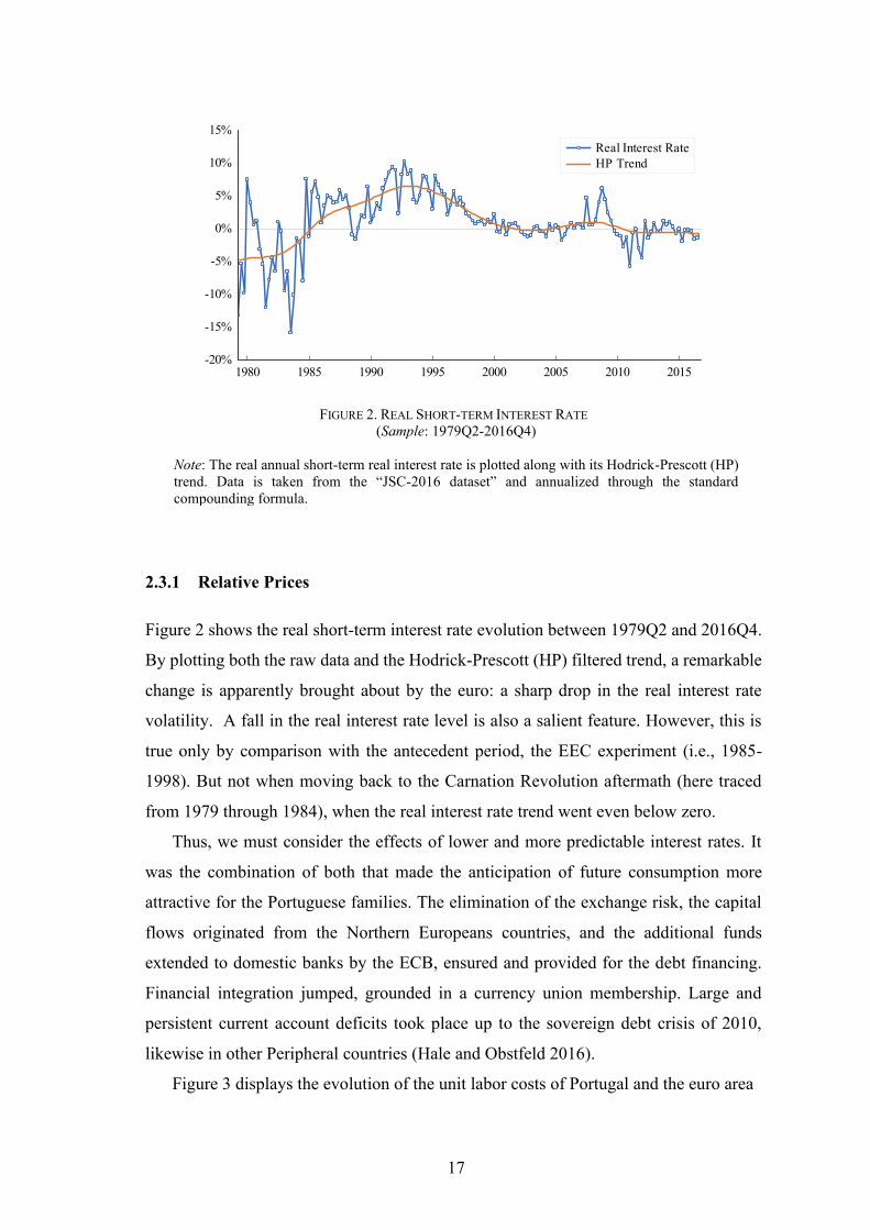
FIGURE 2. REAL SHORT-TERM INTEREST RATE
(Sample: 1979Q2-2016Q4)
Note: The real annual short-term real interest rate is plotted along with its Hodrick-Prescott (HP)
trend. Data is taken from the “JSC-2016 dataset” and annualized through the standard
compounding formula.
2.3.1 Relative Prices
Figure 2 shows the real short-term interest rate evolution between 1979Q2 and 2016Q4.
By plotting both the raw data and the Hodrick-Prescott (HP) filtered trend, a remarkable
change is apparently brought about by the euro: a sharp drop in the real interest rate
volatility. A fall in the real interest rate level is also a salient feature. However, this is
true only by comparison with the antecedent period, the EEC experiment (i.e., 1985-
1998). But not when moving back to the Carnation Revolution aftermath (here traced
from 1979 through 1984), when the real interest rate trend went even below zero.
Thus, we must consider the effects of lower and more predictable interest rates. It
was the combination of both that made the anticipation of future consumption more
attractive for the Portuguese families. The elimination of the exchange risk, the capital
flows originated from the Northern Europeans countries, and the additional funds
extended to domestic banks by the ECB, ensured and provided for the debt financing.
Financial integration jumped, grounded in a currency union membership. Large and
persistent current account deficits took place up to the sovereign debt crisis of 2010,
likewise in other Peripheral countries (Hale and Obstfeld 2016).
Figure 3 displays the evolution of the unit labor costs of Portugal and the euro area

18
60
70
80
90
100
110
1996 1998 2000 2002 2004 2006 2008 2010 2012 2014 2016
Euro Area (19 Countries)
Portugal
FIGURE 3. UNIT LABOR COSTS – HP TREND
(Sample: 1995Q1-2016Q4)
Source: Raw data from OECD.Stat9. HP trends extracted by the author, by running the EViews
application.
from 1995 to 2016. An upward trend is noticeable up to the 2008 global financial crisis,
reflecting increasing wages and anemic productivity growth – a process that has taken
its course since the second half of the 1990s, as pointed out by Blanchard (2007).
Between 2000 and the European sovereign debt crisis of 2010-12, the Portuguese unit
labor costs went even above the euro area average. A sharp downward correction
followed the “sudden stop”10 of capital inflows and the subsequent fiscal and
macroeconomic adjustment program led by the Troika (i.e., the FMI, the ECB, and the
European Commission).
At the origin of wage growth disconnected from improving labor productivity, there
was a change in the relative prices of nontradables to tradables, in turn, motivated by a
demand shift driven by the already mentioned fall in the interest rate and stepping up in
financial integration. With Schmitt-Groh and Uribe (2013), I would emphasize that,
because the law of one price hold for traded goods in a common market, the price effect
of the demand shift translated to the nontradables. Meanwhile, the impact on
9 Data extracted on 02 Feb 2018 20:00 UTC (GMT) from OECD.Stat; http://stats.oecd.org/
index.aspx?DatasetCode=ULC_EEQ. 10 A financial crisis originated by a “sudden stop” of foreign capital inflows as typified by Calvo (1998).

19
competitiveness might have been softened or intensified by the course of the nominal
exchange rate.
Hence, I address now the relative price of the home to foreign currencies averaged
by the pertinent trade weights, that is the nominal effective exchange rate (NEER). To
elicit possible effects from the euro adoption, one must still consider the comovements
of domestic inflation with the foreign counterparts, otherwise the mere evolution of the
nominal exchange rate would be meaningless. Thus, the pertinent question is the
following: Can we find evidence of a regime change in the NEER related with the euro
adoption while having at the backdrop the path of inflation differentials between Portugal
and its foreign counterparts?
A first tentative answer is pursued by plotting the relative purchasing power parity
relation for Portugal across an extended period. Moreover, the per capita output gap11
behavior is also exhibited, bearing in mind the possible Balassa-Samuelson effect12.
This paper “2016 dataset”, spanning from 1979Q2 to 2016Q4, and described in
Appendix C, offers that possibility. To represent the relative purchasing power parity, I
used the same criteria, the trade weights, to compute (i) the inflation differential between
Portugal and its foreign counterparts and (ii) the change in the NEER. To control for the
output gap, I followed an identical procedure, that is making the (log) difference between
the real Portuguese output per capita and its foreign counterparts averaged on the same
basis. Next, I applied the HP filter to extract the trend from the three series, because, and
again, the primary interest is in long-run behavior rather than in high-frequency
movements.
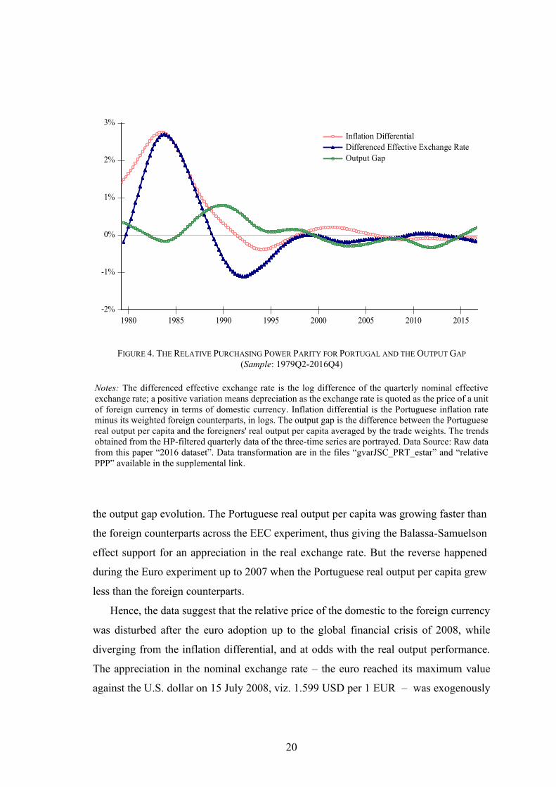
Figure 4 depicts the HP trends for the inflation differential, the change in the effective
exchange rate (NEER), and the output gap. We can see periods where the inflation
differential and the variation in the NEER are tied, suggesting that the relative purchasing
power holds; and periods where they are falling apart, thus hinting relative prices
disturbances. There are two periods when the inflation differential and the change in the
NEER noticeably diverge: between 1987-1997, roughly overlapping the EEC
experiment, and again throughout 1998-2007, that is in the course of the Euro experiment
up to the global financial crisis. However, there is a sharp distinction in what concerns
11 In this context, output gap means the log difference of the home to the foreign the real GDP
counterpart. See, for ex., Pesaran (2007). 12 See, for ex., Froot and Rogoff (1995, Section 3) for a discussion on the Balassa-Samuelson effect.
20
-2%
-1%
0%
1%
2%
3%
1980 1985 1990 1995 2000 2005 2010 2015
Inflation Differential
Differenced Effective Exchange Rate
Output Gap
FIGURE 4. THE RELATIVE PURCHASING POWER PARITY FOR PORTUGAL AND THE OUTPUT GAP
(Sample: 1979Q2-2016Q4)
Notes: The differenced effective exchange rate is the log difference of the quarterly nominal effective
exchange rate; a positive variation means depreciation as the exchange rate is quoted as the price of a unit
of foreign currency in terms of domestic currency. Inflation differential is the Portuguese inflation rate
minus its weighted foreign counterparts, in logs. The output gap is the difference between the Portuguese
real output per capita and the foreigners' real output per capita averaged by the trade weights. The trends
obtained from the HP-filtered quarterly data of the three-time series are portrayed. Data Source: Raw data
from this paper “2016 dataset”. Data transformation are in the files “gvarJSC_PRT_estar” and “relative
PPP” available in the supplemental link.
the output gap evolution. The Portuguese real output per capita was growing faster than
the foreign counterparts across the EEC experiment, thus giving the Balassa-Samuelson
effect support for an appreciation in the real exchange rate. But the reverse happened
during the Euro experiment up to 2007 when the Portuguese real output per capita grew
less than the foreign counterparts.
Hence, the data suggest that the relative price of the domestic to the foreign currency
was disturbed after the euro adoption up to the global financial crisis of 2008, while
diverging from the inflation differential, and at odds with the real output performance.
The appreciation in the nominal exchange rate – the euro reached its maximum value
against the U.S. dollar on 15 July 2008, viz. 1.599 USD per 1 EUR – was exogenously

21
determined, given the negligible size of the Portuguese economy in the euro area (about
2% in GDP terms), and evolved irrespectively of the current account which reached a
negative balance of -12.1% in 200813. Finally, the rise in the inflation differential reflects
the increase in the price of nontradables, driven by the already mentioned demand shock.
2.3.2 The Impact on Productivity
How has the relative prices disturbing course impacted on the Portuguese GDP growth
across the Euro Experiment? I suggest that the answer lies in its interaction with the
Portuguese institutional framework, leading to misallocation of the capital inflows14.
More specifically, the labor market institutions and capital markets development; and
where misallocation is referred both to between-sectors (from tradables to nontradables)
and within-industry. The same mechanism likely impaired foreign direct investment in
the tradables sector, thus hindering GDP growth driven by (efficient) factors
accumulation and productivity improvement. However, this paper does not explore that
possibility, and as such, I restrict the discussion to the twofold misallocation story, that
is the allocative inefficiency between and within sectors.
As pointed out by Rodrik (2008), whereas addressing “countries with low to medium
incomes”15, tradables “suffer disproportionately (that is, compared with nontradables)
from the institutional weakness”; and the “increase in the relative price of tradables [i.e.
currency undervaluation] acts as a second-best mechanism to partly alleviate the relevant
distortion” (p. 6). The argument follows in the opposite direction: an increase in the
relative price of nontradables (i.e. the real exchange rate overvaluation) hits output
growth in case of weak institutions. What makes Portugal different from the “medium
income” countries considered by Rodrik (2008) is the nature of the prevailing
institutional dysfunctionalities. Property rights and the enforcement of contracts are
secure in any euro area member state. Thus, one must look at other sorts of distortions
potentially leading to misallocation of resources.
13 Data from the AMECO, downloaded on 8 May 2018, < http://ec.europa.eu/economy_finance/ameco/
user/serie/ResultSerie.cfmv>. 14Where I put “institutional frictions”, Reis (2013) has put “financial frictions”, after undertaken an
advanced theoretical and empirical approach to the “dismal performance” of the Portuguese economy in
the euro. I leave the discussion of that alternative (possible complemental) to the essay “Puzzling Around
the Euro Experiment”. 15 There is no evidence found for a relationship between currency valuation and economic growth for
richer countries (Rodrik 2008).

22
Earlier works on the dismal performance of the Portuguese performance contain the
answer. After building a model based on the celebrated span-of-control model of Lucas
(1978), Braguinsky et al. (2011) showed that larger and more efficient firms were hit
harder by the high level of employment protection prevailing in Portugal. The so-called
“tax on labor” led to the “incredible shrinking” of the Portuguese firms observed since
the mid-1980s (pp. 1-6). It is worth noting that the effect of the “gross labor tax rate” on
the firm size is non-linear16. As such, overvaluation, meaning increased wages
disconnect from productivity improvement, has an adverse impact on the larger and more
efficient firms.
Therefore, the appreciation of the real exchange rate observed during the Euro
experiment up to the 2010-12 financial crisis hit the tradables through two operative
channels. First by imposing augmented efficiency-adjusted labor costs whereas the price
of traded goods was kept unchanged by the “law of one price”. Second, by amplifying
the “gross labor tax” and as such weighing more on larger enterprises. It should be noted
too that the tradable sector was the one that exhibited catching-up productivity along the
process of structural transformation analyzed between 1956-1995 (Duarte and Restuccia
2007).
Concerning the nontradables, a reference is due to empirical analysis undertaken by
Dias et al. (2016). The within-industry allocative inefficiency was found to go even
further in the nontradables rather than in the tradables17. Over the period 1996–2011, five
industries in the service sector accounted for “72% of the total increase in resource
misallocation” (Dias et al. 2016, p. 48). That might have happened not only due to the
already mentioned non-linear effect of the “labor tax” – I suggest – while impacting on
the firm optimal size, but also throughout the “self-employment” channel. An increase
in the “gross labor tax” increases “the fraction of labor force that chooses to be self-
employed” (Braguinsky et al. 2011, p. 19), further shifting the firm size distribution to
the left and hence lowering aggregate productivity.
16 In the model built by Braguinsky et al. (2011) the effect of the distortionary “tax wage” is non-linear –
meaning that an increase in the “tax results in a disproportional decrease in the sizes of the largest, that is,
the most efficient firms” (p.17) – in spite of having been specified like a linear tax. 17 I suggest an explanation. The demand shock driven by financial integration has been directed to the
nontradables. In the tradable sector, production costs increased whereas selling prices were pinned down
by the “law of one price”. Thus, the shock was harmful all across the firm size distribution for the
tradable sector.

23
Up to now, changes in relative prices have been approached by eliciting stylized facts
as portrayed in Figure 2, for the interest rate; in Figure 3 for the price of nontradables
and tradables while reflected by the evolution of unit labor costs; and finally in Figure 4
for the real exchange rate, while implied by the course of the relative PPP.
It is now time to submit that same hypothesis – a significant intertwined change in
relative prices in Portugal over the Euro experiment – to an empirical test in a more
advanced framework, the GVAR.
3. THE EMPIRICAL MODEL
A formal description of the GVAR modeling approach is offered in Appendix B, but it
seems appropriate to summarize here its basic structure while informing the empiric
model specified in the present work.
3.1 Methodology
The GVAR is defined and implemented in two steps as follows.
First, individual countries VARX* models are built and estimated. A VARX* is a
vector autoregressive model augmented with the foreign variables, the “star variables”.
Hence, the right-hand side of each equation contains not only the lagged values of the
domestic (endogenous) variables but also the current and lagged values of the foreign
variables and a country-specific error term. The foreign variables are treated as weak
exogenous, given that we are dealing with small open economies and are computed as per
the relative weight of each foreign country to the home economy. More formally, let 𝒙𝑖𝑡∗
denote the vector of 𝑘𝑖∗ of foreign variables respecting to country i, where 𝑖 =
0, 1, 2, … , 𝑁, with 0 indexing the numeraire country (i.e., the United States). Each
country-specific foreign variable, 𝑥𝑖𝑡∗ , is defined by the weighted average of that same
domestic variable for all remaining countries in the sample; hence 𝑥𝑖𝑡∗ =
∑ 𝑤𝑖𝑗𝑥𝑗𝑡 , 𝑁𝑗=0 with 𝑤𝑖𝑖 = 0. The weights, 𝑤𝑖𝑗 , 𝑗 = 0, 1, …𝑁, are chosen by using a proxy
for the interdependences in one specific variable, like the trade shares for the real output,
and not necessarily the same for all variables; however the trade shares are the most
commonly adopted and even for averaging financial indicators (e.g., the foreign countries
price of equity). The VARX* coefficients are estimated each country at a time. Given the
24
presence of integrated variables, the estimation is made through a vector error-correcting
model, the VECMX*, and by applying the reduced rank regression method.
Second, the estimated country-specific VARX* models (36 in this paper) are stacked
and after that combined by using a link matrix formed by the weights used to compute the
foreign variables. Thus, the link matrix is the tool for mapping the individual VARX*
coefficients into the coefficients of the global system, and thereby to reexpress all
exogenous foreign variables in the global model in terms of domestic endogenous
variables. Thereby, the GVAR model is identified and can be solved recursively to
undertake the dynamic analysis: impulse response functions, persistence profiles, and
forecasting. Finally, empirical distributions are derived by bootstrapping the GVAR and
are used to statistically evaluate the results obtained from the dynamic analysis and to test
for overidentifying restrictions and structural breaks.
3.2 The Model Specification
In the spirit of Sims (1980), the specification of the empirical global model turns into the
choice of the variables to include in the VARX* individual country models. A choice to
be made in light of the questions addressed, and with parsimony.
The present empirical work is foremost interested in possible relative prices
disturbances after the euro adoption although without disregarding the potential of the
GVAR methodology to undertake the dynamic analysis. Therefore, the choice of
variables includes those entering in the baseline IS/LM model: the output, inflation and
the short-term interest rate18. The justification for the short-term interest rate is reinforced
because its behavior reflects structural interrelationships in a long-run horizon,
subsumable in the relative purchasing power parity (PPP). Section 4.3 below provides a
detailed explanation. The list of variables still includes the exchange rate given that we
are dealing with a currency union and interested in its interlinkages with the rest of the
world. Bearing in mind the role of capital markets as (i) a source of financial shocks and
(ii) a transmission channel of real and nominal macroeconomic disturbances, tracking its
behavior also looks relevant; therefore, the price of equity is included. Finally, the long-
term interest rate completes the list of six endogenous variables.
The inclusion of the IS/LM set of variables looks still justified despite the interest in the
18 See, for ex., Clarida et al. (1999).

25
TABLE 1─VARX* MODEL SPECIFICATION
Variables U.S. model Other countries model
Domestic Foreign Domestic Foreign
Real output per capita
Inflation
Real equity price –
Real exchange rate – –
Short-term interest rate –
Long-term interest rate –
Oil prices (DU) – –
Note: “Other countries model”: A domestic variable will not enter a specific country model in case of
missing observations. Example: The price of equity is not included in the Portuguese model because the
first data value available from the MSCI Country Index is from 1988Q1.
long-run aggregates behavior because both high and low frequencies movements are
intertwined in the data and possibly linked by cointegrating relations.
The six mentioned variables – the real output, the inflation rate, the real price of
equity, the real exchange rate, the short- and the long-term interest rates – are the same
as in Dees et al. (2007a), DdPS hereafter. But for the real output, I used the respective per
capita value19. Likewise, those were the variables selected in the seminal work of Pesaran
et al. (2004). The exception is the long-term interest rate, as the “real money balances”
entered in its place in the original formulation. More formally, the country-specific
variables in this paper GVAR model are defined as follows:
- Real output per capita, 𝑦𝑖𝑡 = 𝑙𝑛(𝐺𝐷𝑃𝑖𝑡/𝐶𝑃𝐼𝑖𝑡) − 𝑙𝑛( 𝑃𝑜𝑝𝑖𝑡), where 𝐺𝐷𝑃𝑖𝑡 stands
for the nominal Gross Domestic Product, is the consumer price index, and
the population resident in country i 20;
19 I suggest that using per capita values for the GDP is beneficial for the identification of the short-run
multipliers in case of a lengthy estimation period, as in this paper whose sample extends over 38 years,
1979(1)-2016(4). For that time span one may find significant differences in population variation even
across developed economies. For example, the cumulative growth of the U.S. population was 45 % over
1979-2016, while only 7% for the UK and 10% for Japan. 20 As detailed in Appendix C, data on country-specific population are normalized by the respective mean.
tUSy ,*
,tUSy ity *
ity
tUS , *
,tUS it *
it
tUSeq , iteq *
iteq
*
,
*
, tUStUS pe − itit pe −
tUSr , itr *
itr
tUSlr , itlr *
itlr
o
tp o
tp
itCPI
itPop

26
- The inflation rate, ;
- The real equity prices, , where is the nominal equity
price index;
- The real exchange rate, , where is the exchange rate
in terms of U.S. dollars;
- The nominal short-term interest rate, , where is the
nominal short-term rate of interest per annum, in percent;
- The nominal long-term interest rate, , where is the
nominal short-term rate of interest per annum, in percent.
The common variable is:
- Oil prices, , where is the price of oil in USD.
Table 1 shows the country-specific VARX models defined by the stated choice of
variables. The models are the same for all countries with exception to the United States,
assumed as the numeraire or “reference country” (Pesaran et al. 2004, p. 130). As such
the exchange rate is included as a domestic variable in all the other countries, but not the
foreign exchange rate (i.e., the “star” variable); the opposite happens with the U.S. model.
Because of its leading role in capital markets, the foreign counterparts of the price of
equity and of the interest rates are not expected to be exogenous in the U.S. model.
Although, and to take due account of second-round effects, the real output and the
inflation rate foreign counterparts are included in the U.S. model.
I chose the dominant unit (DU) option to model oil prices, thus assumed as exogenous
for all economies, including the United States. In the earlier stages of the GVAR
methodology, the oil prices were treated as an endogenous variable within the U.S. model
(Pesaran et al. 2004), (Dees et al. 2007a) and DdPS. It remains as an option still today
(see, for ex., Dees 2016). But the choice here was for the dominant unit formulation
(Chudik and Pesaran 2013), given the growing share of oil consumption outside the
United States.
The lag-length of each VARX* model is selected by applying the Akaike Information
Criterion (AIK). However, and due to data limitations, the maximum order of two is
)/ln( 1, −= tiitit CPICPI
)/ln( ititit CPIEQeq = itEQ
)/ln( itititit CPIEpe =− itE
)100/1ln(25,0 S
itit Rr += S
itR
)100/1ln(25,0 L
itit Rlr += L
itR
)ln( t
o
t POILp = tPOIL

27
TABLE 2 ─ COUNTRIES AND REGIONS IN THE GVAR MODEL
U.S. Euro Area−Core Euro Area−Periphery Rest of Asia
China Germany Italy Indonesia
Japan France Spain Korea
UK Netherlands Ireland Thailand
Belgium Portugal Malaysia
Austria Greece Philippines
Denmark Finland Singapore
Other dev. countries Rest of W. Europe Latin America Rest of the World
Canada Switzerland Brazil India
Australia Sweden Mexico Turkey
New Zealand Norway Chile Saudi Arabia
Peru South Africa
imposed on the domestic variables, , and one on the foreign counterparts, . The selected
lag-lengths are reported in Table A. 2. in Appendix A along with the number of the identified
cointegration relations.
3.3 Data, Sample and Computation Program
This paper version of the GVAR model covers 90% of the world economy as in DdPS.
The main difference rests on treating each euro area member states individually whereas
in the latter the euro area is taken as a whole, that is as a single country/region. “Exploring
the international linkages of the Euro Area” was the object of study in DdPS, while the
focus of the present investigation is disentangling each member state (Portugal, in
particular) from the euro economy.
The GVAR methodology and the respective Toolbox 2.0 (Smith and Galesi 2014)
allows for proceeding with regional aggregations either before or after estimating the
individual countries models. Therefore, the impulse response analysis is entertained in
this paper at the country level for every euro area member; and again for the euro area
Core (EA-Core, hereafter) and the euro area Periphery (EA-Periphery, hereafter) as
separate regions.
ip iq

28
The results of the investigation of Bayoumi and Eichengreen (1992) on the response
to supply and demand shocks across the former European Community member states
provided the base to divide the euro area between the Core and the Periphery. That
division was already strikingly apparent in the quoted work, and premonitory of the
cleavage revealed by the 2008 global financial crisis and the subsequent European
sovereign debt crisis of 2010-12. Austria and Finland, which acceded to the European
Community only in 1995, were not included in the Bayoumi and Eichengreen (1992)
study. However, a more recent investigation in business cycle synchronization across the
European Union presented by Aguiar-Conraria and Joana Soares (2011) provides the
support to ascribe Austria to the EA-Core and Finland to the EA-Periphery.
Finally, and because de facto rather than de jure exchange rates regimes is the relevant
criterion for the present work, I included Denmark in the EA-Core. It should be noted that
the Danish krone is pegged to the euro since the inception of the latter, and according to
the quoted study of Aguiar-Conraria and Joana Soares (2011), Denmark is the second
most synchronized country with the EA-12 members (i.e., the first twelve countries that
joined the European currency union). By using the same methodology, while
investigating the impact of European Monetary Union on business cycle synchronization
across its member states and other European economies, Aguiar-Conraria et al. (2013)
arrived at the same conclusion about the fit of Denmark with the euro area.
Table 2 shows the list of the 36 countries covered in this paper sample and its
distribution through specific regions.
The data is described in Appendix C. The sample spans over 1979Q2-2016Q4, while
in the DdPS was over 1979Q2-2003Q4, later on extended by Mauro and Smith (2013) to
1979Q2-2011Q2 and to 1979Q2-2013Q1 by Smith and Galesi (2014).
Three different time frames were defined for estimating the model: the full sample,
1979Q2-2016Q4; the observation window W1 corresponding to the period 1979Q2-
1998Q4 and the observation window W2 corresponding to the period 1997Q2-2016Q4.
Recall that the euro was launched on 1 January 1999, when the conversation rates of the
founding members' currencies were fixed. Observation window W1 matches precisely to
the period before the euro introduction, 1979Q2-1998Q4. Regarding window W2, the
endpoint corresponds naturally to the final observation in the full sample, 2016Q4. But
for the starting observation, I chose 1997Q2 instead to the first quarter in the euro life,

29
1999Q1, to assemble the same number of data points as in W1 (i.e., 79 observations),
without loss of consistency considering that the process of nominal convergence was
already on course since the mid-1990s.
For the construction of the foreign variables (the "star" variables), I made use of the
trade shares (exports plus imports) to build the weight matrices, given the role of trade
relations on business cycles linkages. However, while in DdPS the weights were based
on the average trade flows computed over the last three years, I used the average over the
full sample.
All routines since the computation of the foreign variables and going through the
range of the preliminary tests have been undertaken by running the “GVAR Toolbox
2.0”(Smith and Galesi 2014)21, as well as the estimation of the country-specific models
and the global VAR; and the subsequent dynamic analysis, and tests for the selected
restrictions.
When reporting the results, the following criteria are adopted:
• The “focus group” comprehend the United States, the EA-Core and the EA-
Periphery regions plus Portugal, the UK and Sweden. The interest in the UK
and Sweden rest on being members of the European Union but not euro adopters
(see: Aguiar-Conraria and Joana Soares 2011; Hashem Pesaran et al. 2007). The
results for the “focus group” are reported in the main text.
• The “extended focus group” comprehend the United States, Japan, the UK, the
12 initial members of the euro area, except Luxembourg, plus Denmark, and the
Rest of Western Europe countries (Switzerland, Sweden and Norway). The
results for the “extended focus group” are reported in Appendix A.
• The remaining countries are reported in the supplemental material.
3.4 Testing for Unit Roots and Weak Exogeneity
The domestic and the foreign counterparts time series, as well as oil prices, were tested
for unit roots, based on the “weighted symmetric estimation” test of the ADF type, as
advocated by DdPS. The full results are available at the “Output” sheet in the
supplemental material. In the case of Portugal, the unit root hypothesis is not rejected at
21 Available at https://sites.google.com/site/gvarmodelling/gvar-toolbox.

30
5% significance level, either for the endogenous variables or for the foreign counterparts
(the “star” variables).
The weak exogeneity of country-specific foreign variables and the common variable
(oil prices) is a fundamental assumption for GVAR modeling. Table A. 3 in Appendix A
shows the results of the of the appropriate test implementation for the “extended focus
group”. The weak exogeneity is not rejected at 5% significance level in most cases. The
exceptions are the output for Spain (borderline) and Finland; and inflation for Belgium,
Austria and Finland; and the price of equity for Austria. It is worth noting that the oil
prices weak exogeneity is not rejected for any country, a result that favors the option of
assuming this variable also as exogenous for the United States.
3.5 Specification Tests and Break Dates
The “GVAR Toolbox 2.0” (Smith and Galesi 2014) include the routines to undertake the
tests for checking the stability of short-run coefficients, including the full set referred in
DdPS (Section 3.5). They were implemented, and the results and critical values are
available at the “Output” file in the supplemental material (see the sheets “str_stab-stats”
and “str_stab_cvals”).
Here it seems of interest to address more specifically the tests designed to identify a
one-time structural change, namely the QLR test for break dates, whereby suggesting
inflection points in the variables of the model. Moreover, testing for break dates in the
context of the GVAR entails an advantage when compared with single-equation models
because of the cobreaking events (Hendry and Mizon 1998), which are accounted for in
the former but not in the latter, as also highlighted by Dees (2016).
Table A. 4, inserted in Appendix A, reports the QLR break dates for the “extended
focus group”. The following breaks were identified for the Portuguese variables: 1985Q1
for the real output; 1985Q2 for the inflation rate; 2003Q3 for the real exchange rate;
1985Q2 for the nominal short-term interest rate; and 2010Q4 for the nominal long-term
interest rate. The latter comes without surprise: it is related to the European sovereign
debt crisis of 2010-12 (Shambaugh 2012). As does the break detected for “real exchange
rate” while matching the currency regime change implied by the “Euro experiment”.
However, the results for the real output and the nominal variables, that is the inflation rate
31
and the nominal short-term interest rate, do not look as straightforward and deserve
further examination.
Given 17 years of GDP stagnation observed after the euro adoption, a break date
connected with the “Euro experiment” is expected rather than with the “EEC
experiment”. Recall that the “EEC experiment” went on through 1985-1998, and the real
output break detected in this paper model is on 1985Q1. To interpret this result, one
should bear in mind that in the GVAR framework the behavior of the foreign counterparts
is accounted for when identifying a break date. By inspecting Table A. 4 again, we can
see that there are also break dates identified for the U.S. real output in 1985 as well as for
Netherlands and Italy. For Germany, a break is detected in 1991, thus one year after the
Reunification. When plotting the real GDP behavior of those economies along with those
of Portugal, as depicted in Figure A. 1 in Appendix A, we can see that, whereas 1985 is
associated with an upward trend in the real GDP growth rate for Portugal, it stands for a
turning point towards a decline for the other countries mentioned. We should now look
to what happens around 2008-2010, that is after the eruption of the global financial crisis.
Now the Portuguese GDP behavior grossly matches the downward trend observed in the
other countries output, and there is no break date identified. Because the GVAR technique
accommodates the cobreaking, it makes clear when international linkages or endogenous
factors are responsible for regime changes in the macroeconomic variables.
4. EMPIRICAL RESULTS
I now present the main results obtained from the specified empirical model, starting with
the short-term impacts, moving next to the impulse response functions and finally to the
analysis in the long run.
4.1 Contemporaneous Effects
In the individual VARX* model, the domestic variables are regressed on their
contemporaneous foreign counterparts averaged by the trade weights. Given that all
variables enter in logs, the associated coefficients − the diagonal elements of matrix
in equation (B.1), in Appendix B − can be interpreted as impact elasticities between the
domestic and foreign variables, as highlighted by Dees et al. (2007b, p. 16); thus
0iΛ

32
providing insights on the degree of interlinkages across real, monetary and financial
aggregates in the international setting.
Table A. 5 inserted in Appendix A reports the estimated contemporaneous
coefficients over 1979Q2-2016Q4 for the “extended focus group”. It is worth highlighting
the main findings and to compare with the DdPS results; however, the latter referred to
the period 1979Q2-2011Q2 as provided by Mauro and Smith (2013, Table 2.5).
• Real output coefficient. This paper estimates for the U.S., Japan, and the UK
coefficients are close to those of Mauro and Smith (2013, Table 2.5).
Respectively: 0.64 versus 0.61; 0.76 versus 0.79; and 0.69 versus 0.90. As already
mentioned, the euro area is specified as a single VARX* model in the
DdPS/Mauro and Smith (2013), whereas their member states are modeled
individually in the present work. Hence, I suggest comparing the results of Mauro
and Smith (2013) with those found here for the larger euro area economies. That
means 0.60 shown in Mauro and Smith (2013, Table 2.5) for the euro area versus
0.96 shown here for Germany and 0.45 for France.
• Inflation rate coefficient. Again, this paper estimates compare fairly well with
DdPS/Mauro and Smith (2013) for the United States, Japan and the UK. However,
while the estimated coefficient for the euro area is 0.23 in Mauro and Smith (2013,
Table 2.5), here it is 0.57 for Germany and 0.49 for France, the latter possibly
reflecting the covariance across the euro area member states.
• Equity price coefficient. In this paper the estimated values are 1.13 for Germany
and 0.99 for France, which compare with 1.04 for the euro area in Mauro and
Smith (2013, Table 2.5). It should be noted that a value of one means that 1%
change in the foreign equity prices translates in 1% change in domestic equity
prices in the same quarter. Moreover, we can see high significant estimates across
all countries as shown by the Newey-West t-ratio statistic also reported in Table
A. 5. Overall this indicates that the GVAR model captures quite well the price of
equity comovements; and thereby reflecting the close linkages in capital markets
across the developed economies. The impulse response analysis in Section 4.2
points towards the same direction.
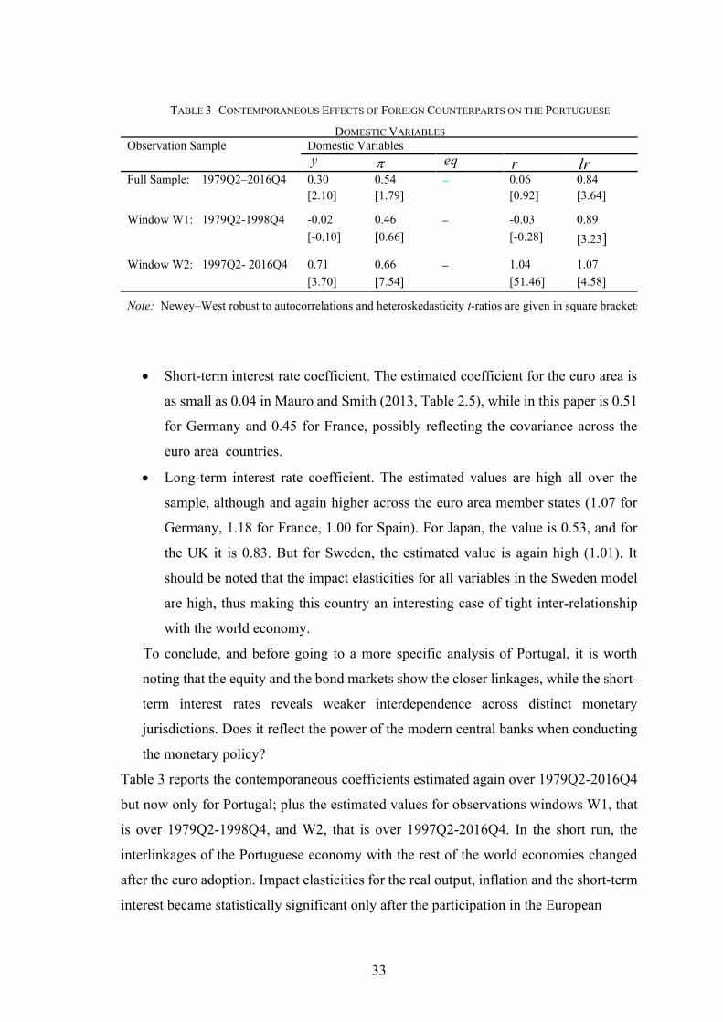
33
TABLE 3−CONTEMPORANEOUS EFFECTS OF FOREIGN COUNTERPARTS ON THE PORTUGUESE
DOMESTIC VARIABLES
PORTUGAL
•
Observation Sample Domestic Variables
Full Sample: 1979Q2–2016Q4 0.30 0.54 − 0.06 0.84
[2.10] [1.79] [0.92] [3.64]
Window W1: 1979Q2-1998Q4 -0.02
0.46 − -0.03 0.89
[-0,10] [0.66] [-0.28] [3.23] Window W2: 1997Q2- 2016Q4 0.71 0.66 − 1.04 1.07
[3.70] [7.54] [51.46] [4.58]
Note: Newey–West robust to autocorrelations and heteroskedasticity t-ratios are given in square brackets.
• Short-term interest rate coefficient. The estimated coefficient for the euro area is
as small as 0.04 in Mauro and Smith (2013, Table 2.5), while in this paper is 0.51
for Germany and 0.45 for France, possibly reflecting the covariance across the
euro area countries.
• Long-term interest rate coefficient. The estimated values are high all over the
sample, although and again higher across the euro area member states (1.07 for
Germany, 1.18 for France, 1.00 for Spain). For Japan, the value is 0.53, and for
the UK it is 0.83. But for Sweden, the estimated value is again high (1.01). It
should be noted that the impact elasticities for all variables in the Sweden model
are high, thus making this country an interesting case of tight inter-relationship
with the world economy.
To conclude, and before going to a more specific analysis of Portugal, it is worth
noting that the equity and the bond markets show the closer linkages, while the short-
term interest rates reveals weaker interdependence across distinct monetary
jurisdictions. Does it reflect the power of the modern central banks when conducting
the monetary policy?
Table 3 reports the contemporaneous coefficients estimated again over 1979Q2-2016Q4
but now only for Portugal; plus the estimated values for observations windows W1, that
is over 1979Q2-1998Q4, and W2, that is over 1997Q2-2016Q4. In the short run, the
interlinkages of the Portuguese economy with the rest of the world economies changed
after the euro adoption. Impact elasticities for the real output, inflation and the short-term
interest became statistically significant only after the participation in the European
y eq r lr

34
FIGURE 5. GENERALIZED IMPULSE RESPONSE OF A NEGATIVE UNIT (1 S.E.) SHOCK TO U.S. REAL EQUITY
PRICES ON REAL OUTPUT PER CAPITA (BOOTSTRAP MEAN ESTIMATES WITH 90% BOOTSTRAP ERROR
BOUNDS).
currency union. Furthermore, they were pretty aligned with the remaining member states
estimated values (see Table A. 5, in Appendix A).
4.2 Impulse Response Analysis
Within the GVAR framework, the generalized impulse response function (GIRF), a
technique summarized in Appendix B, traces the dynamic effects across all economies of
a shock to one variable. The shocks can be originated in an individual country or
simultaneously in all countries of a given region, or even at the global level. A shock to
a common variable, like the oil prices, is also considered global.
This paper reports five shocks, implemented over the full sample 1979Q2-2016Q4,
as follows: (i) a negative shock to U.S. real equity prices; (ii) a positive shock to oil prices
(iii) a positive shock to U.S. short-term interest rate; (iv) a negative shock to EA-Core
real equity prices; (v) a positive shock to U.S. real output. The first three shocks are the
same as in DdPS, and the fourth is new; the fifth does not look as informative but is still
reported. It is worth noting that a statistically non-significant impulse response function
may either reflect an identification limitation or a feebler degree of international
interactions across one particular variable (in case, the real output) or combination of both
effects.
Figure 5 displays the GIRFs for a negative shock to U.S. equity prices on real output

35
FIGURE 6. GENERALIZED IMPULSE RESPONSE OF A POSITIVE UNIT (1 S.E.) SHOCK TO OIL PRICES ON
INFLATION (BOOTSTRAP MEAN ESTIMATES WITH 90% BOOTSTRAP ERROR BOUNDS).
across the “focus group” countries. The size of the shock is one standard error, which is
equivalent to a fall of around 5-6% in the U.S. real equity prices per quarter. The impact
is more pronounced in Portugal than in the EA-Periphery as a whole: the real output
decline in the fourth quarter is by 0.9% in Portugal versus 0.7% in the EA-Periphery; and
the average over the following quarters is 1.8% versus 1.3%, respectively. The same
pattern is evidenced when entertaining shocks to the EA-Core equity prices and to oil
prices (see the “Output” file in the supplemental material). Why is the (lag) sensitivity of
Portuguese output to external shocks higher than the remaining countries in the euro
area22? This question deserves further investigation, but that behavior might be related
with nominal and real rigidities in the labor market.
Figure 6 displays the GIRFs for a positive shock to oil prices on inflation across the
“focus group” countries. The size of the shock is one standard error, which represents
around 10-11% increase per quarter in the price of oil. On impact, the effects are stronger
in the United States than in the euro area, likewise in DdPS. However, they are not
statistically significant for Portugal. The inflation rate was much higher in Portugal than
in the other developed countries before the euro adoption. More specifically, the mean of
the rate of inflation over 1979Q2- 2016Q4 was1.7% per quarter for Portugal while being
22 See “Median Estimates” sheet in the Output file ( \gvarJSC\GIRFs\UNITED STATES 1se neg shock to
REAL EQUITY PRICES), available in the supplemental material, to check the persistence of the
response of the shock across all euro area members and Denmark, and comparing with Portugal.

36
FIGURE 7. GENERALIZED IMPULSE RESPONSE OF A POSITIVE UNIT (1 S.E.) SHOCK TO U.S. SHORT-TERM
INTEREST RATE ON LONG-TERM INTEREST RATES (BOOTSTRAP MEAN ESTIMATES WITH 90% BOOTSTRAP
ERROR BOUNDS).
Note: Interest rates are measured on a quarterly basis.
0.5% for Germany and 0.8% for France; and around 1.2% for Italy and Spain. Hence, the
estimation of the regression coefficients in the inflation equation turns more imprecise
for Portugal.
Figure 7 displays the GIRFs for a positive shock to the U.S. short-term interest rate
on long-term interest rates across the “focus group” countries. The size of the shock is
one standard error, which is equivalent to an increase of 0.18% in the U.S. short-term rate
measured on quarterly bases, that is a rise of 72 basis points. The effects on the long-term
interest rate are statistically significant and are roughly the same for the United States,
the UK, the EA-Core and EA-Periphery, including Portugal, and converging to 0.10%
around the 12th quarter.
Figure 8 displays the GIRFs for a negative shock to the EA-Core real equity prices
on the real exchange rate across the five countries of the “focus group” plus China23. The
size of the shock is one standard error, which is equivalent to a fall of around 4-5% per
quarter in the average equity prices across the EA-Core member states. Although having
implemented the model over the full sample, that is from 1979Q2 through 2016Q4, the
23 Recall that the real exchange rate is not in the list of the U.S. endogenous variables. Thus, Figure 8
portrays the GIRF for China, the world's second largest economy, in place of the United States.

37
FIGURE 8. GENERALIZED IMPULSE RESPONSE OF A NEGATIVE UNIT (1 S.E.) SHOCK TO EA-CORE REAL
EQUITY PRICES ON THE REAL EXCHANGE RATE (BOOTSTRAP MEAN ESTIMATES WITH 90% BOOTSTRAP
ERROR BOUNDS).
GIRFs for the real exchange rate in the EA-Core and EA-Periphery, including Portugal,
are quite similar. That behavior possible reflects the dynamics of the nominal
convergence triggered by the Maastricht Treaty24. It seems worth noting the contrasting
profile of the real exchange rates of both Sweden and the UK. This differentiated pattern
fits well the empirical evidence on their “diachronic business cycles” shown in Aguiar-
Conraria and Joana Soares (2011) and in Aguiar-Conraria et al. (2013).
Figure 9 displays the GIRFs for a positive shock to the U.S. real output on the real
output across the “focus group” countries. The size of the shock is one standard error,
which is equivalent to an increase of around 0.5% per quarter in the U.S. real output. The
responses are not statistically significant for the “focus group” countries other than the
United States, thus contrasting with the results shown in Mauro and Smith (2013, p. 29).
Even for the United States, they are different. While, in this paper, the estimated increase
in the output is 0.36% over the first year, it amounts to 0.7% in Mauro and Smith (2013,
p. 29). It should be noted that oil prices are a global variable in both model’s specification.
But, in this paper, it was defined as a dominant variable, while entered as an endogenous
variable in the U.S. model, Mauro and Smith (2013). Furthermore, the real output is
24 The Maastricht Treaty was signed in 1992, but the implied stabilization of the nominal exchange rates
across the European Union member states started after 1994. As noted by Bayoumi and Eichengreen
(2018), in 1992 and again in1993, the European Exchange Rate Mechanism (ERM) was hit by the crisis
involving the UK and Italy, and finally France. Portugal joined the ERM in April 1992.

38
FIGURE 9. GENERALIZED IMPULSE RESPONSE OF A POSITIVE UNIT (1 S.E.) SHOCK TO U.S. REAL OUTPUT
PER CAPITA ON REAL OUTPUT PER CAPITA (BOOTSTRAP MEAN ESTIMATES WITH 90% BOOTSTRAP ERROR
BOUNDS).
measured differently, as I used the per capita units, as already mentioned. Finally, his
paper sample spans over a lengthy period, namely 1979Q2-2016Q4 versus 1979Q2-
2011Q2 in Mauro and Smith (2013).
4.3 Analysis of Long Run
Within the GVAR framework, we may test for long-run equilibrium relationships, such
as the purchasing power parity (PPP), by imposing the pertinent overidentifying
restrictions on the cointegrating vectors25.
Therefore, the strategy envisaged to test the impact of the euro adoption on the
Portuguese relative prices was to impose the appropriated restriction successively over
the sampling periods separated by the euro adoption 1999Q1. In this case, the
observations windows W1, defined between 1979Q2 and 1998Q4 and W2, defined
between 1997Q2 and 2016Q4, where the starting point in the latter is 1997Q2, instead of
1999Q1, to assemble the same number of observations.
However, after estimating and depicting the persistence profiles with regard to sample
W1 (see Figure 10) and to sample W2 (see Figure 11), it became apparent the difficult
adjustment to the long-run equilibrium when the model is implemented over to the
25 See, for ex., Smith and Galesi (2014, pp. 130-32).

39
1979Q2-1998Q4
FIGURE 10. PERSISTENCE PROFILE OF THE EFFECT OF SYSTEM-WIDE SHOCKS TO THE
COINTEGRATING RELATIONS.
OBSERVATION WINDOW W1: 1979Q2-1998Q4.
Notes: Persistence profiles bootstrap median estimates portrayed for the “extended focus group”, under
the exact identification scheme of the cointegrating vectors. The number of cointegration relations for
the individual country models was determined under the GVAR modeling standard routine (Case IV).

40
1997Q2-2016Q4
FIGURE 11. PERSISTENCE PROFILE OF THE EFFECT OF SYSTEM-WIDE SHOCKS TO THE
COINTEGRATING RELATIONS.
OBSERVATION WINDOW W2: 1997Q2-2016Q4.
Notes: Persistence profiles bootstrap median estimates portrayed for the “extended focus group”, under
the exact identification scheme of the cointegrating vectors. The number of cointegration relations for
the individual country models was determined under the GVAR modeling standard routine (Case IV).

41
observation Window W2. Moreover, that disturbance is observed across all developed
countries. I rechecked the cointegration ranks by changing the specified number of
cointegration relations, but without any indication of improvement. And there was no
evidence of eigenvalues greater than one. Finally, the empirical model run over the
observation Window W2 was the same as the one run over observation Window W1.
Therefore, I concluded that the instability was ingrained in the data, not the outcome of a
misspecified empirical model26.
All considered I made the following decision. To evaluate the long-run equilibrium
relationships over the observation window W1, 1979Q2-1998Q4, that is the period
preceding the euro adoption, and then again over the full sample, 1979Q2-2016Q4, that
is now incorporating the “Euro experiment”. This strategy was somewhat inspired by the
Dees (2016) approach to the study of the impact of the 2008 global financial crises on the
interrelation of financial variables with business cycles. Dees (2016) estimated a GVAR
model over the full sample 1987-2013. After that, compared the results with those
obtained from a restricted sample, where the post-financial crisis period was excluded,
that is an observation window defined between 1987-2007.
The next step was to estimate, after imposing the restriction of interest, in case the
PPP condition, the specified empirical model over the two selected periods and test
whether the restriction is or is not rejected in any of those periods. And as such, gathering
statistical evidence, related to the euro adoption, about possible deviations from the
equilibrium level of the real exchange rate.
The current version of the GVAR Toolbox (Smith and Galesi 2014) does not allow
to test the absolute PPP27. However, the relative PPP can be tested using the well-known
property that the relative PPP is implied by the uncovered interest parity (UIP) and by the
Fisher inflation parity (FIP) relations combined. This paper pursues in that direction,
without disregarding the sensitivity of the relative PPP measure to the base year (Rogoff
26 The global financial crisis of 2008 likely accounts for the data instability turned apparent by the
persistence profiles exhibited in Figure 11 (i.e., for the observation Window W2). Bayoumi and
Eichengreen (2018), in a paper revisiting the conditions for the European countries to constitute an
optimum currency area, made the choice to exclude the year of 2009 from the sample when analyzing the
correlation shocks across U.S. regions and across the euro area countries (p. 7). 27 The PPP long-run relation is testable within the GVAR framework after proper transformations as
made by Dees et al. (2007a, pp. 7-9), even though not included in the current version of the GVAR
Toolbox routines (Smith and Galesi 2014, p. 131).

42
1996)28. But, at the same time, benefiting from including the interest rate into the test
formulation, in addition to the inflation and the nominal exchange rates variables, that is
the three relative prices of interest.
Recall that the relative PPP is defined by:
(1)
where is the (log) effective exchange rate, 29, and where
is the (log) bilateral exchange rate of country i with country j.
In a world of perfect foresight, equation (1) can be written for the expected variation
on the nominal effective exchange rate as a function of country i expected inflation
differential to its foreign counterparts
*
1,1,
*
1,1,1, +++++ −=−= tititititi EEEeeE (2)
Now notice that UIP relationship, which must hold by a simple arbitrage argument
(Obstfeld and Rogoff 1996, p. 528), is given by
*
, 1 , 1 , 1i t i t i tr r E ee+ + += +
(3)
where is the nominal interest rate defined in period for period .
Now combining (2) and (3):
(4)
which imply the FIP relationship and that the real interest rate holds across countries.
Finally, and again with an arbitrage argument, we can see that once verified
simultaneously the UIP and the FIP conditions the relative PPP necessarily holds.
The stochastic formulations30 for the UIP and the FIP conditions are given by:
28 As the relative PPP compares the rate of growth of the variables of interest (the nominal exchange rate
and inflation) it overcomes the problem of dealing with prices indexes possible based on different basket
of goods across countries. See Rogoff (1996) for a discussion on this subject. 29For computational purposes note that:
30 See Garratt et al. (2006, Chapter 4).
itee ==
N
j ijijit ewee0
jtitij eee −=
1, +tir t 1+t
**
0000 ititit
N
j ijitjt
N
j ijit
N
j ij
N
j ijijit eeeweewewewee −=−=−== ====
*
1,
*
1,1,1, ++++ −=− titititi ErEr
*
ititit ee +=
*
, 1 , 1 , 1i t i t i tE ee r r+ + + = −

43
(5)
(6)
In practical terms, the implementation of the test depends on the number of
cointegration relations identified. More commonly, the rank of order 2 is found, by which
the FIP and the UIP conditions are simultaneous imposed and tested. When the rank order
is of 1, we run one test at a time. For rank order of 3, we select a third possible structural
relationship to run the overidentifying test. As noted by Smith and Galesi (2014, p. 132),
“one cannot test for two long-run relations and simply exactly identify the remaining
cointegration relation”. The output gap non-divergent hypothesis stands as one
possibility. In the terms formulated by Pesaran (2007), the cointegrating vector for the
domestic and the foreign real output per capita – the y and y* time series – take the form
(1, -1). In a somewhat mild version, the coefficient respecting to the home country is left
unrestricted, as such just subsuming a “common trends in output” (see Bernard and
Durlauf 1995, p. 99). I have opted for the latter considering the diversity of countries in
the sample. Thus, whenever having to impose a third overidentifying restrictions, the
following econometric formulation is adopted 31:
(7)
where the intercept is restricted to lie in the cointegration space32 to allow for the joint
evaluation of the three overidentifying restrictions implied in equations (5), (6) and (7).
Table A. 6 presents the results of the tests undertaken over observation window W1
and the full sample. That is the log-likelihood ratio statistic (LR statistic) and the bootstrap
critical values after imposing the UIP and the FIP conditions, and the output gap
restriction in case of the rank order of 3. It should be noted that the cointegrating vectors
are identified at each country VECMX models (see equation (B.8) in Appendix B).
For Portugal, the number of cointegrating vectors identified was of 3 for the
observation window W1, 1979Q2-1998Q4, and 2 for the full sample, 1979Q2-2016Q4.
Thus, three overidentifying restrictions (UIP, FIP and the output gap) were
simultaneously imposed over the observation window W1. Those restrictions were not
31 The same specification can be seen in Assenmacher and Pesaran (2008, p. 13). 32 This means to choose Case II for the treatment of the deterministic component in the estimation of the
VECMX* individual models (see Section B.4 in Appendix B).
3ia
)0(~,222, Iar tiiitiit +=−
)0(~,11
* Iarr tiiitit +=−
)0(~,33
*
3, Iayy tiiititi +=−

44
rejected given that the LR statistics is of 66.9, which compares with the critical values of
82.8 (5% significance level) and of 98.6 (1% significance level). Conversely, when
running the test over the full sample, thus including the Euro experiment, the FIP and the
UIP conditions are rejected. In this case, the LR statistic is 76.7, whereas the critical
values are 52.7 (5% significance level) and 62.1 (1% significance level).
To conclude, the relative PPP holds in the period prior to the introduction of the euro,
1979Q2-1998Q4, and is rejected when evaluated over an extended period that includes
the Euro experiment, 1979Q2-2016Q4.
4.4 Robustness
Using the full sample instead of the observation window W2 to evaluate the FIP and
the UIP long-term equilibrium entails a limitation that needs to be checked. I have
considered two alternative approaches. First, to rerun the program over observation
window W2 but excluding the year 2009 from the sample, given that the global financial
crisis of 2008 is the likely source of the instability detected through the persistent profile
analysis. Second, making a third observation window, say W3, by enlarging observation
window W2 backwards.
The first approach rendered non-converging persistence profiles again. Thus, I moved
to the second one. The period of the new observation window, W3, was defined between
1985Q3 and 2016Q4, considering the break date of 1985Q2 identified both for the
Portuguese inflation and interest rates, as reported in Section 3.5. After running the
overidentifying restriction test, the UIP and the FIP are again rejected. The LR statistics
is of 84.5, which compares with the bootstrap critical values of 52.3 (5% significance
level) and 62.8 (1% significance level).
To conclude, when including the Euro experiment in the period of test – both in the
full sample, 1979Q2-2016Q4, as in the observation window W3, 1985Q3-2016Q4 – the
relative PPP, subsumed in the UIP and the FIP relations, is rejected. The robustness of
the evaluation benefits from changing the initial observation, here moved from 1979Q2
to 1985Q3, given the sensitivity of the relative PPP measure to the base year (Rogoff
1996), as already noted.

45
5. CONCLUSION
After comparing the stagnation of the Portuguese economy throughout 1999-2016 with
the successful participation in the EFTA and the EEC, I raised, with a Marshallian flavor,
a first hypothesis for the dismal performance in the euro: The change in relative prices
after relinquishing monetary policy autonomy.
But there has been an intriguing issue since the beginning of this inquiry – the length
of the stagnation (17 years). And we have learned with North (1994), and with Daron
Acemoglu and co-authors (2005; 2001), that, in the long run, institutions play a decisive
role in economic performance.
Therefore, I faced two research questions, requiring different methodologies, and
ultimately, a connection, if it is the case. Looking for evidence on a regime change in
relative prices requires a quantitative analysis. I started by eliciting stylized facts where a
shift in the price of future to present consumption became evident; and a correlated
episode of overvaluation. I moved then to a more advanced framework, the GVAR. I
tested the relative PPP, which holds before the euro adoption, but is rejected when the
data sample is extended to include the euro period. Turning now to the institutional
framework. I noted that the Carnation Revolution of 1974 was followed by a severe
incident of property rights violation in 1975 and an anti-market ideology grasped the new
Constitution, approved in 1976. The accession to the European Community in 1986 led
to the re-establishment of the basic free-market rules, including the plain safeguard of
property rights. However, the bias against larger enterprises and the highest degree of
labor protection among the developed countries remained as a legacy of the original
Constitution.
How did those macroeconomic events, underpinned by the financial integration in the
euro area, and the prevailing institutional framework interact? The augmented version of
the celebrated span-of-control of Lucas (1978), proposed by Braguinsky et al. (2011),
contains the answer. By modeling employment protection as a “gross-tax on labor”,
Braguinsky et al. (2011) showed that employment protection decreases the firm optimal
size. I argued that the impact of overvaluation was higher the larger (and more efficient)
the enterprises, on account of the “gross-tax on labor”. Therefore, on top of the well-
known between-sector adverse impacts, overvaluation leads to within-industry

46
misallocation of resources. The empirical evidence on declining allocative efficiency
within-industry, between 1996 and 2011, has been found by Dias et al. (2016). This
closes the explanation for the dismal performance of the Portuguese economy in the euro.
In sum, it stemmed from the interaction of a regime change in relative prices with
domestic “institutional frictions”.
A note on policy implications. The short-run dynamics analysis conducted with the
GVAR has shown that Sweden notably exhibits fast responses to external shocks, in sharp
contrast with the sluggish Portuguese adjustments. Given that Sweden is widely
recognized as equity prone, I suggest that economic development in Portugal would
improve if equity and efficiency trade-offs were less conditioned by the old anti-market
ideology. The fit with the European currency union would also improve by softening the
labor market rigidities and the bias against larger enterprises.

47
APPENDIX A
Tables and Figures
TABLE A. 1− PORTUGUESE REAL GDP GROWTH BREAK DATES, 1961Q1-2016Q4
Dependent Variable: Real Output per Capita Annual Growth Rate for Portugal
Method: Least Squares with Breaks
Date: 01/19/18 Time: 20:45
Sample (adjusted): 1961Q1 2016Q4
Included observations: 224 after adjustments
Break type: Bai-Perron tests of L+1 vs. L sequentially determined breaks
Breaks: 1974Q2, 1985Q2, 2001Q1
Selection: Trimming 0.15, Sig. level 0.05
Variable Coefficient Std. Error t-Statistic Prob.
1961Q1 - 1974Q1 -- 53 obs
C 0.065402 0.003422 19.11277 0.0000
1974Q2 - 1985Q1 -- 44 obs
C 0.010999 0.003756 2.928648 0.0038
1985Q2 - 2000Q4 -- 63 obs
C 0.034259 0.003139 10.91542 0.0000
2001Q1 - 2016Q4 -- 64 obs
C 0.002532 0.003114 0.813018 0.4171
R-squared 0.489357 Mean dependent var 0.027994
Adjusted R-squared 0.482394 S.D. dependent var 0.034626
S.E. of regression 0.024912 Akaike info criterion -4.529267
Sum squared resid 0.136530 Schwarz criterion -4.468345
Log - likelihood 511.2779 Hannan-Quinn criter. -4.504676
F-statistic 70.27658 Durbin-Watson stat 0.351897
Prob(F-statistic) 0.000000
Notes: Structural change analysis of the Portuguese real GDP per capita annual growth rate by applying the
Bai (1997) and Bai and Perron (1998) methods to identify break dates. EViews output.

48
TABLE A. 2–VARX* LAG LENGTH-ORDER AND NUMBER OF COINTEGRATION RELATIONS
Countries Full Sample Window W1 Window W2
# cnt # cnt # cnt
U.S. 2 1 2 2 1 2 2 1 3
Japan 2 1 2 2 1 3 1 1 1
UK 2 1 1 2 1 3 2 1 1
EA-Core
Germany 2 1 2 1 1 3 1 1 2
France 2 1 2 2 1 2 2 1 2
Netherlands 2 1 2 1 1 4 2 1 2
Belgium 1 1 2 1 1 3 2 1 1
Austria 1 1 4 1 1 3 2 1 4
Denmark 2 1 1 2 1 2 2 1 2
EA-Periphery
Italy 2 1 2 1 1 2 1 1 2
Spain 2 1 2 1 1 2 2 1 3
Ireland 2 1 2 2 1 3 2 1 2
Portugal 2 1 2 2 1 3 2 1 2
Greece 1 1 1 2 1 2 2 1 3
Finland 2 1 1 2 1 1 2 1 3
Other Europeans
Switzerland 2 1 1 1 1 2 1 1 1
Sweden 2 1 2 2 1 2 1 1 2
Norway 2 1 4 2 1 2 1 1 4
Notes:
1) The number of cointegration relations was identified by using the standard option – Case IV – as
expressed in Equation (B.21) in Appendix B, by which the trend is restricted to lie in the
cointegration space 33.
2) Further to the full sample period, 1979Q2-2016Q4, the number of cointegration relations for
Window W1, 1979Q2-1998Q4, and for Window W2, 1997Q2-2016Q4, are also reported for the
sake of interpretation of the Persistence Profiles portrayed in the main text.
33 For a discussion on the different options, see, for ex., Garratt et al. (2006, pp. 118-22).
( )ii qp ,
ip iq ip iq ip iq

49
TABLE A. 3− F-STATISTICS FOR TESTING THE WEAK EXOGENEITY OF THE COUNTRY-SPECIFIC
FOREIGN VARIABLES AND OIL PRICES, 1979Q2-2016Q4
Country Foreign Variables and the Oil Prices
U.S. F(2,136) 0.15 5.68 − 1.03 − − 2.41
Japan F(2,132) 0.36 0.19 0.03 − 2.20 0.88 0.63
UK F(1,133) 0.00 2.51 1.06 − 1.12 1.48 2.66
EA-Core
Germany F(2,132) 0.10 1.26 0.35 − 0.42 0.40 0.50
France F(2,132) 1.03 1.81 0.12 − 2.96 1.19 0.32
Netherlands F(2,132) 0.09 0.57 0.92 − 0.28 1.16 0.79
Belgium F(2,132) 0.94 5.47† 0.72 − 0.99 0.21 2.04
Austria F(4,130) 0.56 2.95† 4.48† − 1.89 0.64 1.35
Denmark F(1,135) 1.20 0.70 0.07 − 0.11 3.55 2.63
EA-Periphery
Italy F(2,132) 0.45 1.39 0.23 − 1.95 0.78 0.37
Spain F(2,132) 3.13† 1.48 0.06 − 1.71 0.76 0.80
Ireland F(2,133) 1.94 0.80 0.46 − 1.19 1.62 0.16
Portugal F(2,133) 0.81 0.14 3.29 − 0.23 0.14 0.94
Greece F(1,135) 0.032 0.08 0.61 − 0.15 0.02 1.48
Finland F(1,134) 4.00† 4.56† 0.44 − 2.61 0.53 2.86
Other Europeans
Switzerland F(1,133) 0.51 0.97 0.00 − 0.43 0.21 1.42
Sweden F(2,132) 2.74 0.71 0.37 − 0.07 1.07 0.31
Norway F(4,130) 2.12 2.42 0.92 − 0.14 0.30 1.39
Note: †denotes statistical significance at 5% level.
*y* *eq ** pe − *r *lr op

50
TABLE A. 4−STRUCTURAL STABILITY TESTS: BREAK DATES FOR QLR TESTS, 1979Q2-2016Q4
y π eq e-p r lr
U.S. 1985Q1 2002Q1 1998Q4 − 1985Q1 1987Q4
Japan 1989Q4 1986Q3 1992Q3 1998Q3 1986Q3 1996Q1
UK 1987Q1 1985Q4 1987Q1 1988Q4 1985Q3 1985Q1
EA-Core
Germany 1991Q1 1990Q4 1987Q1 2002Q4 1985Q3 1985Q3
France 1991Q4 1986Q1 1985Q2 1986Q4 1985Q4 1985Q1
Netherlands 1985Q3 1993Q2 1989Q1 1988Q4 1985Q4 1985Q1
Belgium 1991Q4 1998Q3Q3 2008Q2 2003Q2 1985Q2 1987Q4
Austria 1988Q1 1985Q3 2003Q4 2006Q1 1986Q2 1988Q2
Denmark 1988Q3 1986Q3 1986Q3 1989Q3 − −
EA-Periphery
Italy 1985Q3 1985Q3 1986Q2 2003Q3 1987Q4 1986Q3
Spain 1991Q4 1988Q4 1986Q2 1988Q4 1988Q1 1987Q2
Ireland 2011Q2 1985Q2 − 2003Q3 1985Q1 2010Q1
Portugal 1985Q1 1985Q2 − 2003Q3 1985Q2 2010Q4
Greece 1986Q2 1985Q3 2003Q3 1994Q3 −
Finland 1987Q2 1985Q1 2000Q2 2003Q3 1986Q3 −
Rest of W. Europe
Switzerland 1987Q2 1985Q1 1986Q4 1987Q1 1989Q2 1992Q1
Sweden 1986Q1 1990Q1 1985Q3 2004Q1 1992Q3 1987Q1
Norway 1985Q1 2002Q4 1990Q4 2006Q1 1995Q1 1990Q3
Note: The QLR test is the Wald form of the Quandt (1960) likelihood ratio statistics. See Dees et al.
(2007b: Section 3.5) for its application in the GVAR context.

51
TABLE A. 5−CONTEMPORANEOUS EFFECTS OF FOREIGN VARIABLES ON THEIR DOMESTIC
COUNTERPARTS, 1979Q2-2016Q4
Country Domestic Variables
U.S. 0.64 0.15 − − –
[5.00] [1.73]
Japan 0.76 0.10 0.71 -0.05 0.53
[3.33] [1.07] [6.74] [-1.02] [7.11]
UK 0.69 0.70 0.81 0.25 0.83
[4.02] [6.42] [17.04] [2.04] [9.16]
EA-Core
Germany 0.96 0.57 1.13 0.51 1.07
[4.12] [4.76] [19.44] [3.46] [15.64]
France 0.45 0.49 0.99 0.45 1.18
[3.41] [4.19] [19.13] [4.97] [17.27]
Netherlands 0.17 0.57 0.95 0.23 0.88
[1.26] [7.42] [15.18] [3.88] [24.18]
Belgium 0.51 0.94 0.96 0.34 0.69
[4.04] [8.32] [8.60] [3.45] [10.21]
Austria 0.22 0.49 0.92 0.50 0.90
[1.64] [5.40] [7.78] [5.63] [12.04]
Denmark 0.66 0.29 0.79 − −
[3.49] [2.01] [14.71]
EA-Periphery
Italy 0.68 0.04 1.09 0.25 0.69
[5.54] [0.35] [10.96] [4.10] [4.59]
Spain 0.72 0.59 0.99 0.12 1.00
[4.11] [3.36] [13.41] [1.38] [4.71]
Ireland 0.88 0.65 − 0.90 1.27
[2.05] [2.90] [3.50] [7.06]
Portugal 0.30 0.54 − 0.06 0.84
[2.10] [1.79] [0.92] [3.64]
Greece 1.61 0.55 − 0.10 −
[5.41] [3.22] [0.58]
Finland 1.13 0.48 1.04 0.48 −
[5.41] [4.54] [7.94] [3.87]
Rest of W. Europe
Switzerland 0.25 0.28 0.87 0.15 0.54
y eq r lr

52
[3.81] [2.83] [16.12] [2.16] [8.48]
Sweden 1.30 1.03 1.13 0.51 1.01
[4.96] [5.66] [14.76] [3.38] [6.25]
Norway 0.51 0.58 1.11 0.13 0.70
[3.25] [1.85] [14.74] [1.67] [6.61]
Note: Newey–West robust to autocorrelations and heteroskedasticity t-ratios are given in square brackets.
TABLE A. 6−LR STATISTICS FOR TESTING OVERIDENTIFYING RESTRICTIONS
Country Window W1: 1979Q2-1998Q4 Full Sample: 1979Q2-2016Q4
Rank
LR
Statistic
95%
Crt.Values
99%
Crt.Values Rank LR
Statistic
95%
Crt.Values
99%
Crt.Values
Germany 3 116.7 85.8 98.9 2 93.1 68.2 71.3
France 2 64.9 80.7 96.0 2 75.1 66.2 79.5
Italy 2 98.5 79.9 88.9 2 61.5 77.0 86.6
Spain 2 96.7 77.9 86.7 2 72.6 68.1 75.9
Portugal 3 66.9 82.8 98.6 2 76.7 52.7 62.1
UK 2 71.1 73.1 79.8 2 82.1 70.1 75.0
Sweden 2 45.9 77.1 84.1 2 63.3 54.8 67.0
Notes: The “LR statistic” stands for the log-likelihood ratio statistic. “Crit. Values” are the bootstrap
critical values. Cointegration relations: when the rank is of 2, the FIP and UIP conditions have been
imposed; when the rank is of 3, the FIP the UIP and the output gap conditions have been imposed.
Selected countries: the bigger economies in the EA-Core and in the EA-Periphery; plus Portugal, and
the European countries non-members of the euro area but included in the “focus group” (the UK and
Sweden).

53
FIGURE A. 1. ANNUAL REAL GDP PER CAPITA GROWTH RATE (HP TREND)
Notes: Source: author computation using the EViews’ Hodrick-Prescott filter routine. Raw data: quarterly
data from gvar-JSC dataset.
-2%
-1%
0%
1%
2%
3%
4%
5%
6%
1980 1985 1990 1995 2000 2005 2010 2015
USA Portugal Netherlands
Italy Germany

54
APPENDIX B
THE GVAR METHODOLOGY
A formal description of the GVAR methodology is presented here. The purpose is to
highlight the building blocks and the results further suited to the empirical model
introduced in the main text. There will be nothing new in relation to the standard
approach, as originally offered by Pesaran et al. (2004)34, and more recently reviewed by
Chudik and Pesaran (2016); but a more detailed approach to oil shocks, while treated as
a dominant unit variable in the sense defined by Chudik and Pesaran (2013).
B. 1 The VARX* Country-specific Models
Given a set of 𝑁 + 1 countries indexed by 𝑖 = 0,1,2, … ,𝑁 and where 0 states for the
numeraire country, the country i second order VAR model with weak exogenous
variables35, VARX* (2, 2), is written as
(B.1)
where is a vector of domestic variables, is a vector of foreign
variables, and is a vector of idiosyncratic country-specific shocks, for .
The vector of foreign variables is defined as
(B.2)
with , , a set of weights such that . The weights are more
commonly based on the trade share of country j in country i (imports plus exports) even
when dealing with financial variables, e.g. in Dees (2016). Although, to capture more
specific and time-varying financial interlinkages a more elaborated criterion might be
34 See Mauro and Smith (2013) for a compact presentation or Smith and Galesi (2014) for a more
detailed description. 35 For a definition of I (1) weakly exogenous variables see, for ex., Garratt et al. (2006, pp. 56-59).
itx 1ik *
itx 1* ik
itu Tt ...,,2,1=
ijw Nj ...,,2,1,0= 10
= =
N
j ijw
=
==N
j
iijtijit ww0
* 0,xx
ittiitiiititiitiiiiit t uxΛxΛxΛxΦxΦaax +++++++= −−−−
*
2,2
*
1,1
*
02,21,110

55
required, e.g. in Favero (2013)36. More variations in weighting schemes are offered by
Eickmeier and Ng (2013).
In matrix notation (B.1) is written as
(B.3)
where is the matrix of country-specific weights and
is vector collecting all endogenous variables in the global
model; as such .
The idiosyncratic shocks are assumed to be serially uncorrelated with mean 0 and
allowed “to be correlated across regions [countries] to a limited degree” (Pesaran et al.
2004; 131) – a feature to which we will revert later.
The vector autoregression expressed in (B.1) might be rewritten for the first difference
of whenever containing at least one-unit root37:
(B.4)
where
We now define , and . Assuming
that cointegration exists within and between and , is a rank deficient
matrix, and the error correction representation of (B.1) is given by
(B.5)
To avoid quadratic trends in the level of variables (Pesaran et al. 2004: 137)38, must
36 In Favero (2013) weights are based on the distance among fiscal fundamentals (expected deficit and
debt ratios to GDP). 37 See, for ex., Hamilton (1994, p. 549) for an alternative representation of a VAR (p) process. 38 See the demonstration in Pesaran et al. (2000, pp. 295-98).
jii wW~ *
ikk
( )'''
1
'
0 ...,,, Ntttt xxxx = 1k
==
N
i ikk0
itu
itx
( ) 211 iiki iΦΦIΦ −−
( ) 2101 iiii ΛΛΛΛ ++
( )'*'' , ititit xxz = ( ) ( )( )1,1 iii ΛΦΠ − ( )22 , iii ΛΦΓ −
itx itx *
itx iΠ
( )*
iii kkk +
1ia
ittiiittiiiiit t uzΓxΛzΠaax +++−+= −− 1,
*
101,10
( ) ( )
ittii
tiiititiitiiiiti t
uxΛ
xΦxΛxΛxΦaax
++
−++−+=
−
−−−
*
1,2
1,2
*
0
*
1,1,10, 11
xWx'* ~iit =

56
be restricted such that , where is a vector39. Insofar, (B.5) is
written as
(B.6)
(B.7)
Under the assumption that the long-run multiplier matrix is of rank , we can
write , where is the loading matrix and is the matrix
of cointegrating vectors, both of full column rank, and get the final form of the VECMX*
model for each individual country
(B.8)
To see how cointegration is articulated both within and between and , and
hence across and for , can be partitioned into conformable to
(Smith and Galesi 2014: 127); as such the error-correction terms can be written as
(B.9)
each country-specific VECMX* is estimated separately through the reduced- rank
regression40 procedure (Pesaran et al. 2004, pp. 137-38) taking in due account the stated
cointegration structure and the weakly exogeneity of foreign and of global variables.
To recover each country VARX* model from the corresponding estimated VECMX*
is straightforward: using (B.7) and the definitions of and we reexpress (B.8) in
levels
39 Given the assumption that is rank deficient, can be estimated from the reduced form
coefficients. See Garratt et al. (2006, p. 120). 40 For a description of the reduced rank ML estimation method see, for ex., Lütkepohl and Krätzig (2004,
pp. 96-103).
iii γΠa =1 iγ ( ) 1* + ii kk
iΠ ii kr
'
iii βαΠ = iα ii rk iβ ( ) iii rkk + *
itx itx *
itx
itxjtx ji
iβ ( )''
*
' , ixix ββitz
ir
iΠ iΓ
( ) ( )
ittitiiit
iiiititiitiiiiit t
uxΛxΦxΛ
γΠγΠxΛxΦxγΠax
+−−+
−++−++=
−−
−−−
*
1,121,2
*
10
*
1,11,1,0 11
iΠ iγ
( ) ( )tt iiitixitixiiti γβxβxβγzβ'*'
*
'' −+=−
( )( ) ittiiititiiiiit t uzΓxΛγzβαcx +++−−−= −− 1,
*
101,
'
0 1
γΠac iii += 00
( )( ) ittiiititiiiit t uzΓxΛγzΠcx +++−−−= −− 1,
*
101,0 1

57
Finally, recalling the restriction and after further simplifications we obtain
equation (B.1).
B. 2 Solving for the GVAR
To build the global model all estimated individual countries VARX* models will be
stacked in a single system which must be solved for , , endogenous
variables, , making use of link matrices that will provide a mapping of the parameters
estimated in the VARX* models into the GVAR coefficients.
Following Smith and Galesi (2014, pp. 136-37), the country i VARX* model
introduced in (B.1) is reexpressed as of order ,
(B.10)
It should be noted that in empirical applications lag length-orders of domestic and of
foreign variables, p and q, are chosen using the Akaike Information Criterion (AIC) or
the Schwarz Bayesian criteria (SBC).
Defining , a vector with dimension , and making ,
(B.10) is rewritten as
(B.11)
with
for
and where and are dimensional matrices; and is non-singular.
Define the link matrices
iii γΠa =1
k =N
ikk0
itx
( )ii qp ,
( )'*'' , ititit xxz = ( ) 1* + ii kk ii qp =
( ) ( ),,,, 00 ijijijiki iΛΦAΛIA =−= ipj ...,,1=
0iAijA ( )*
iii kkk + 0iA
( ) kkk ii + *
1,1,1100 ... iptiiptiiiiiti iit uzAzAaazA +++++= −−
1
*
,
*
1,1
*
0,1,110
...
......
iqtiiq
tiiitiptiiptiiiiit
ii
iit
uxΛ
xΛxΛxΦxΦaax
+++
+++++++=
−
−−−

58
(B.12)
where is the dimensional selection matrix that select , namely and
is the weight matrix introduced in (B.3).
Consequently, we may substitute in (B.11) for and get rid of the exogenous
variables, , while preserving the VARX* coefficients already estimated. Meanwhile, I
provide an illustration of a link matrix that might be useful.
Let be the link matrix for country , and assume a model with only three
country-specific endogenous variables41, e.g. the real output per capita , the inflation
rate , and the nominal short-run interest rate ; as well as a weighting scheme based
on constant weights, and a set of countries:
𝐖1 = , 𝐱𝑡=
Let us use the definition and accordingly reexpress equation (B.11):
41 To be denoted as in Smith and Galesi (2014, p. 18) and as used in our empirical model in next section.
iE ikk itxtiit xEx '=
iW~
itz tixW
*
itx
1W 1=i
ity
itDp itr
1+N
Nwww
ww
ww
11210
1210
1210
0000000
00000000
00000000
0000100000
0000010000
0000001000
N
t
t
t
t
t
t
t
t
t
r
r
Dp
y
r
Dp
y
r
Dp
y
1
2
2
2
1
1
1
0
0
0
tiit xWz =
( ),~, ''
iii WEW =
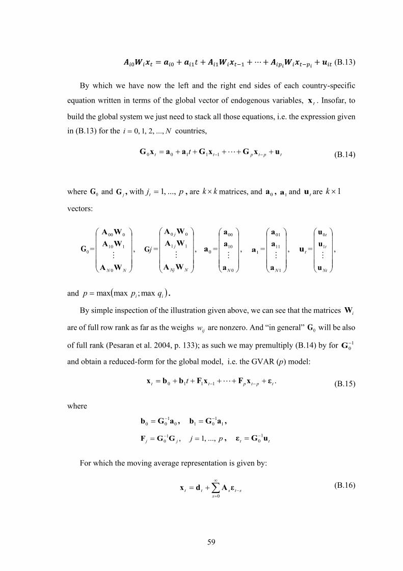
59
𝜜𝑖0𝑾𝑖𝒙𝑡 = 𝒂𝑖0 + 𝒂𝑖1𝑡 + 𝜜𝑖1𝑾𝑖𝒙𝑡−1 +⋯+ 𝜜𝑖𝑝𝑖𝑾𝑖𝒙𝑡−𝑝𝑖 + 𝒖𝑖𝑡 (B.13)
By which we have now the left and the right end sides of each country-specific
equation written in terms of the global vector of endogenous variables, . Insofar, to
build the global system we just need to stack all those equations, i.e. the expression given
in (B.13) for the countries,
(B.14)
where and , with , are matrices, and , and are
vectors:
= , = , = , = , = ,
and .
By simple inspection of the illustration given above, we can see that the matrices
are of full row rank as far as the weighs are nonzero. And “in general” will be also
of full rank (Pesaran et al. 2004, p. 133); as such we may premultiply (B.14) by for
and obtain a reduced-form for the global model, i.e. the GVAR (p) model:
(B.15)
where
, ,
,
For which the moving average representation is given by:
(B.16)
tx
Ni ...,,2,1,0=
0GjG pjt ...,,1= kk 0a
1a tu 1k
0G
NN WA
WA
WA
0
110
000
jG
NNj
j
j
WA
WA
WA
11
00
0a
0
10
00
Na
a
a
1a
1
11
01
Na
a
a
tu
Nt
t
t
u
u
u
1
0
( )ii qpp max;maxmax=
iW
ijw 0G
1
0
−G
0
1
00 aGb −= 1
1
01 aGb−=
pjjj ...,,1,1
0 == −GGF tt uGε 1
0
−=
=
−+=0s
ststt εAdx
.1110 tptptt t εxFxFbbx +++++= −−
tptptt t uxGxGaaxG +++++= −− 11100

60
where represents the deterministic component of , and can be derived
recursively as
(B.17)
with , for
B. 3 Short-Run Dynamics
The high dimensionality of the GVAR model turns unpractical the identification of the
structural innovations using the “structural VAR” methodology (Pesaran et al. 2004, pp.
135-36). I can exemplify with the empirical model presented in Section 3 of the main
text, where there were 187 variables42. Now notice that the identification of the shocks
requires restrictions43, thus amounting to 17,391 in this case. One may
suggest that theoretical motivation to impose restrictions within each country can be
replicable. Nevertheless, there would be still cross-countries interactions to consider.
Thus, shock identification will always be a “problematic” task in the global VAR
framework as emphasized by Chudik and Pesaran (2016, p. 176).
A slightly different story happens when employing the Orthogonalized Impulse
Responses (OIR) of Sims (1980), although restricting the ordering of variables to a single
country. To exemplify this procedure a reference is made to Dees et al. (2007b) where
the OIR technique was employed to measure the effects of shocks to the short-term
interest rates on inflation after ordering the U.S. variables.
All considered, the alternative method to undertake the impulse response analysis in
the GVAR context44 lays on the Generalized Impulse Response Functions (GIRF)
originally proposed by Koop et al. (1996) and applied later on by Pesaran and Shin (1998)
both to the unrestricted and to cointegrated VAR models. By moving in that direction, the
need to identify the “structural innovations” is circumvented. The reduced form error
42 The panel data set comprehend 36 countries and six endogenous variables, but there was not data
available for all variables in every country. To check the list of variables per each country a reference is
made to the sheet “Specification & Estimation of Individual Models” in the file “gvarJSC”, available at
the supplemental link. 43 See, for ex., Hamilton (1994, p. 332) for the identification of structural VARs. 44 The forecast error variance decomposition (FEVD) is also suitable in the GVAR context, while
conditioning on the non-orthogonalized shocks, see for ex. Smith and Galesi (2014, pp. 142-43). The
method will not be reviewed here as it will not be employed in our empirical study.
td tx sA
0AIA ==sk
,0
0s
( ) 2/1−kk
....,2,1,...2211 =+++= −−− spspsss AFAFAFA

61
terms are elected as the source of disturbances to the GVAR system, but after integrating
out the effects of other shocks given the historically observed distribution of the errors
(Pesaran and Shin 1998, p. 19).
Therefore the trigger of the “conceptual experiments” − as in the words of Koop et al.
(1996, p. 121) when referring to the impulse response functions (IRF)s – will be the
regression residuals , where states for the equation in the country. We can
exemplify this with a shock to the U.S. short-term interest rate (an observable variable),
indistinguishably of whether prompted by an “innovation” in the monetary policy domain
or by a change in fiscal policy; or with a shock to the U.S. real output irrespectively of
being originated by demand or supply (unobservable) shocks, which might even have
occurred outside the U.S. economy; or still with a global shock to the equity markets,
which might be entertained simultaneous hitting the price of equity equations error terms
respecting to all countries included in the GVAR model. It remains clear now that while
the GIRF approach does not elicit the original source of a macroeconomic or financial
disturbance, it remains a suitable tool to reveal how those disturbances are transmitted
(the intensity and time path) to the others aggregates within and across countries and
regions. Summing up, the GIRFs are an appropriate technique to study empirically short-
term dynamics, eliciting how different countries react after having being hit by the same
shock. For example, it illustrates how the Portuguese real output or the inflation rate
responds to an equity price shock in the United States in comparison the EA-Core or to
other Peripheral countries.
I present next the formal definition of the GIRF. Let us revert to the system expressed
in (B.14) where the GVAR equations were still written in terms of the individual countries
variables error terms, . Then, the GIRFs are defined as:
,
where is the information set representing the history of the economy up to time
, is the size of the shock, and where “ is the diagonal element of the variance-
covariance matrix corresponding to the equation in the country, and n is the
horizon” (Smith and Galesi 2014, p. 140).
ilu l thl thi
ilu
( ) ( ) ( )11, ,,; −+−+ −== tnttlliiiltntiltt EuEnuGIRF xxx
1−t 1−t
llii,llii,
uΣthl thi
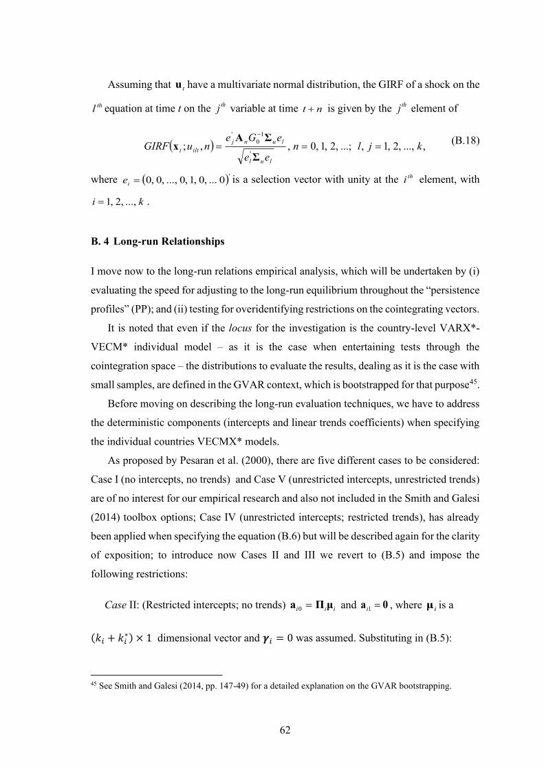
62
Assuming that have a multivariate normal distribution, the GIRF of a shock on the
equation at time t on the variable at time is given by the element of
(B.18)
where is a selection vector with unity at the element, with
.
B. 4 Long-run Relationships
I move now to the long-run relations empirical analysis, which will be undertaken by (i)
evaluating the speed for adjusting to the long-run equilibrium throughout the “persistence
profiles” (PP); and (ii) testing for overidentifying restrictions on the cointegrating vectors.
It is noted that even if the locus for the investigation is the country-level VARX*-
VECM* individual model – as it is the case when entertaining tests through the
cointegration space – the distributions to evaluate the results, dealing as it is the case with
small samples, are defined in the GVAR context, which is bootstrapped for that purpose45.
Before moving on describing the long-run evaluation techniques, we have to address
the deterministic components (intercepts and linear trends coefficients) when specifying
the individual countries VECMX* models.
As proposed by Pesaran et al. (2000), there are five different cases to be considered:
Case I (no intercepts, no trends) and Case V (unrestricted intercepts, unrestricted trends)
are of no interest for our empirical research and also not included in the Smith and Galesi
(2014) toolbox options; Case IV (unrestricted intercepts; restricted trends), has already
been applied when specifying the equation (B.6) but will be described again for the clarity
of exposition; to introduce now Cases II and III we revert to (B.5) and impose the
following restrictions:
Case II: (Restricted intercepts; no trends) and , where is a
(𝑘𝑖 + 𝑘𝑖∗) × 1 dimensional vector and 𝜸𝑖 = 0 was assumed. Substituting in (B.5):
45 See Smith and Galesi (2014, pp. 147-49) for a detailed explanation on the GVAR bootstrapping.
tu
thlthj nt +
thj
( )'0...,0,1,0...,,0,0=iethi
ki ...,,2,1=
iii μΠa =0 0a =1i iμ
( ) ,...,,2,1,...;,2,1,0,,;'
1
0
'
kjlnee
eGenuGIRF
lul
lunj
iltt ===
−
Σ
ΣAx

63
(B.19)
Case III: (Unrestricted intercepts; no trends) and ; again is
assumed. Substituting in (B.5)
(B.20)
Case IV: (Unrestricted intercepts; restricted trends) and .
Substituting in (B.5),
(B.21)
which will take the form already shown in (B.6) whenever making likewise
:
B. 4.1 Persistence Profiles
Persistence profiles (PPs) refer to the time path of a cointegrating relations adjustment to
its long-term equilibrium after being hit by a system-wide or a variable-specific shock.
Given a well-specified model, the persistence profiles analysis gives us insights on
different aspects of the behavior of an economy. For example, Pesaran and Shin (1996)
have found that the adjustment process in the purchasing power parity (PPP) is much
slower than in the uncovered interest parity (UIP). Based on the results of the empirical
model presented in the main text, when estimated for different while successive
observation windows, W1 for 1979Q2-1998Q4 and W2 for 1997Q2-2016Q4, I suggest
that persistence profiles can also offer evidence of structural changes or disturbing events
occurring at a regional or even a global scope. While the adjustment to the equilibrium
was smooth and fast in Window W1 it displays a rough pattern in Window W2 across all
countries in the “extended focus group”. I have made the conjecture that the global
financial crisis of 2008 was the source of the detected instability.
A formal definition for the persistence profiles (PP) will be presented next. But before
it is worth noting that the PPs are invariant to the error terms orthogonalization schemed
00 ia 0a =1i 0γ =i
00 ia iii γΠa =1
iiii γΠac += 00
( )( ) ittiiititiiiit t uzΓxΛγzΠcx +++−−−= −− 1,
*
101,0 1
ittiiittiiiiiit t uzΓxΛzΠγΠax +++−+= −− 1,
*
101,0
ittiiittiiiit uzΓxΛzΠax +++−= −− 1,
*
101,0
.1,
*
101, ittiiittiiiiit uzΓxΛzΠμΠx +++−= −−
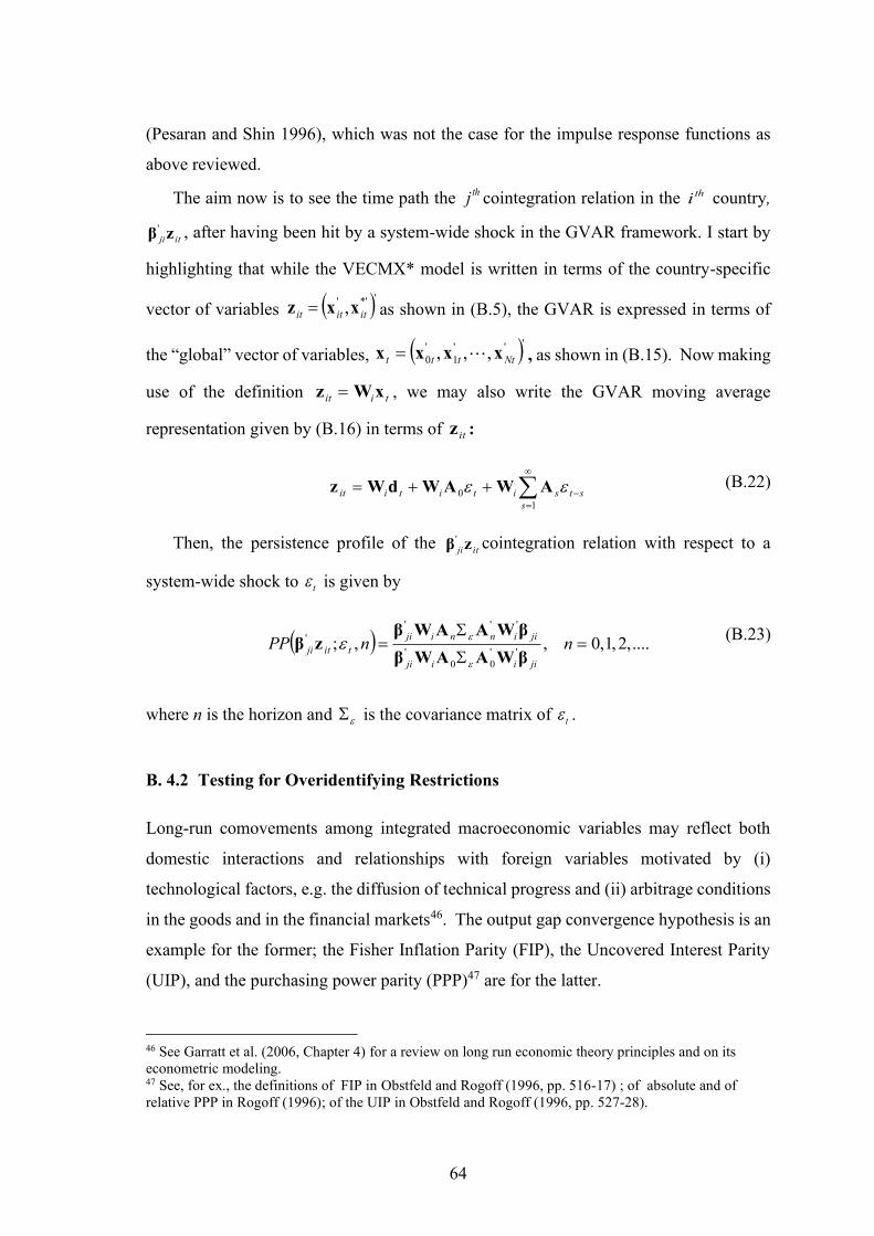
64
(Pesaran and Shin 1996), which was not the case for the impulse response functions as
above reviewed.
The aim now is to see the time path the cointegration relation in the country,
, after having been hit by a system-wide shock in the GVAR framework. I start by
highlighting that while the VECMX* model is written in terms of the country-specific
vector of variables as shown in (B.5), the GVAR is expressed in terms of
the “global” vector of variables, , as shown in (B.15). Now making
use of the definition , we may also write the GVAR moving average
representation given by (B.16) in terms of :
(B.22)
Then, the persistence profile of the cointegration relation with respect to a
system-wide shock to is given by
(B.23)
where n is the horizon and is the covariance matrix of .
B. 4.2 Testing for Overidentifying Restrictions
Long-run comovements among integrated macroeconomic variables may reflect both
domestic interactions and relationships with foreign variables motivated by (i)
technological factors, e.g. the diffusion of technical progress and (ii) arbitrage conditions
in the goods and in the financial markets46. The output gap convergence hypothesis is an
example for the former; the Fisher Inflation Parity (FIP), the Uncovered Interest Parity
(UIP), and the purchasing power parity (PPP)47 are for the latter.
46 See Garratt et al. (2006, Chapter 4) for a review on long run economic theory principles and on its
econometric modeling. 47 See, for ex., the definitions of FIP in Obstfeld and Rogoff (1996, pp. 516-17) ; of absolute and of
relative PPP in Rogoff (1996); of the UIP in Obstfeld and Rogoff (1996, pp. 527-28).
thj thi
itjizβ'
( )'*'' , ititit xxz =
( )'''
1
'
0 ,,, Ntttt xxxx =
tiit xWz =
itz
itjizβ'
t
t
( ) ....,2,1,0,,;''
00
'
'''
' =
= nnPP
jiiiji
jiinniji
titjiβWAAWβ
βWAAWβzβ
=
−++=1
0
s
stsititiit AWAWdWz

65
Such being the case, the pertinent I(1) variables will be cointegrated, meaning that
they share a structure that ties their behavior in an interrelated path. However, a myriad
of disturbing events will originate deviations across time from the long-run equilibrium.
But if that underlining structure exists, the changes on the levels of the cointegrated
variables observed period after period will reflect both the short-term vanishing
disturbances and the reversion to the path “dictated” by the underlining structure. As it is
well known from the cointegration theory, after the seminal contributions of Granger
(1983) and of Engle and Granger (1987), the distinction of the short-run dynamics from
the long-run multipliers is attainable by including an error correction term, here denoted
by , in the first-differenced vector autoregressive model, as expressed in (B.5)48.
Otherwise, the first-differenced representation would not be even a “compatible” with the
cointegration hypothesis (Engle and Granger 1987)49.
The question to be raised next is the following: How to identify in this framework the
long-run relations among the variables of the model? Recall that is a
matrix of rank , and that we can write , where is the loading
matrix and is the matrix of cointegrating vectors, both of rank .
However and are not separately identified50. Thus, to identify we have to
impose restrictions per each cointegrating vectors, thus amounting to restrictions.
A “statistical” solution for this problem can be find through the orthogonalization of ,
in line with Johansen (1988; 1991) approach, which provides an exactly identified
48 In GVAR context, the left-hand side of the VEC model is written in terms of the vector , namely
, while the error-correction term is defined in terms of vector , where xit∗′ are
weakly exogenous. This is because only the so-called conditional model, i.e. the one written for the
differenced data , is considered; while the marginal model, i.e. the one that would be written for the
differenced data , is discarded. The conditional and the marginal models combined form the extend
VECM for . As shown, for example, in Garratt et al. (2006, pp. 135-36) the splitting of the extended
model into those above mentioned marginal and conditional models is based on the (testable) assumption
that the country specific foreign variables are long-run forcing for the endogenous variables
.
49 See Hamilton (1994, pp. 571-73) for a summary demonstration. 50 See Garratt et al. (2006, pp. 36-7) for a detailed explanation.
1, −tiizΠ
iΠ ( )*
iii kkk +
ii kr '
iii βαΠ = iα ii rk
'
iβ ( )*
iii kkr + ir
iα'
iβ'
iβ
ir ir2
ir
'
iβ
itx
itx ( )'*'' , ititit xxz =
itx*
itx
itz
=1
*
titx
=1titx

66
system. Notice that this procedure – to be based on the identity matrix51 in the context of
the GVAR estimation – does not reveal the “original” cointegrating vectors, for which it
stands just as a linear combination. An alternative to identify might be provided by the
economic theory whereby must be supplemented in addition to the r restrictions
arising from normalization. Continuing in this direction, Pesaran and Shin (2002)
described the methods for the identification of the cointegration coefficients based on
information drawn from the economic theory, and for hypothesis testing, in particular
testing for overidentifying restrictions on the cointegrating vectors. Previously and also
in the context of non-stationary time series, Johansen and Juselius (1994, p. 10) had
already addressed the “identification of economic structure in a statistically well-specified
model” yet defining the concept of “economic identification” in a broader perspective,
related to the “economic interpretability of the estimated coefficients”; and offered an
empirical application to the Australian economy, where overidentifying restrictions have
been used to investigate the conformity of long-rung macroeconomic theoretical
relationships, in case drawn from the IS−LM model, with the observed data.
Testing for overidentifying restrictions is a procedure to be used in the present paper
when addressing its fundamental questions related with the dismal path of the Portuguese
economy after the euro adoption. There is statistical evidence of relative price
disturbances in that same period as suggested in a preliminary quantitative approach
presented in the main text
It seems convenient to summarize the “mechanics” of testing for overidentifying
restriction the present context. I would suggest that it can be seen as combination of the
“statistical” with the “economic” identification of the cointegrating vectors. The former
by providing a “benchmark” – the maximum likelihood estimation, given the usual
Gaussian assumptions – defined by the model estimated under the “exact identification”
solution provided by the identity matrix; the latter by setting the framework to model the
long-run relationships which are aimed to be verified empirically, and leading to the
“overidentification” of matrix .
51 To impose the identity matrix the dimensional matrix is partitioned such that the
first block is the identity matrix of order , i.e. where is a
dimensional matrix of coefficients to be estimated.
'
iβ
rri −2
iβ
( )*
iii kkr + '
iβ
ir '' : iKri I ββ = '
iKβ ( )iiii rkkr −+ *

67
A comparison between the results obtained from the “overidentified” versus the
“exact identified” matrices was then undertaken, using the appropriate statistics (the Wald
test) and the pertinent distributions. Accordingly, a judgment is made about the
plausibility of the hypothetical long-run relationship prevalence in the observed period.
To be clear, the point is not to identify the matrix based on theoretical insights, but
rather to test if certain theoretical properties hold in a certain period of time for a given
economy.
I present next the formal description of testing for overidentifying restrictions 52 using
as an illustration the VECM* model with the three endogenous variables, e.g. the real
output per capita, the inflation rate and the short-term interest rate, and the respective
country-specific foreign counterparts, . Suppose now that our
aim is testing for the FIP and the UIP arbitrage conditions, and for the non-divergent
output gap hypothesis in the sense defined by Pesaran (2007). Assuming that the FIP and
the UIP conditions are not trended, and that and are cotrending, after duly testing
for, the deterministic trend coefficient will be absent of the cointegration space. Suppose
however that in the case of the FIP relation we choose to leave unrestricted the inflation
rate coefficient. Translating into an econometric formulation those long-run relationships
will be represented by the following reduced form53 error correction terms, respectively
for the UIP, the FIP and the output gap conditions:
(B.24)
(B.25)
(B.26)
To which corresponds the following (transposed) matrix of cointegrating vectors
52 The topic A.11 “Testing for overidentifying restrictions on the cointegrating vector” in Smith and
Galesi (2014, pp. 130-32) and Chapter 9 in Garratt et al. (2006) provide the basic information to test for
overidentifying restrictions. 53 See in Garratt et al. (2006, Chapter 4) the derivation of the structural long-run equations.
'
iβ
( )'*** ,,,,, ititititititit ryry =z
ity *
ity
)0(~,33
* Iayy tiiitit +=−
)0(~,11
* Iarr tiiitit +=−
)0(~,2222, Iar tiiitiit +=−

68
B.27)
Now notice that we have imposed 17 restrictions in while nine would be enough
to exactly identify . To make it more clear, let us write the exactly identified matrix
based on the identity matrix
(B.28)
We can now estimate the VECM* model using in alternative the and the
options. We should expect that the more restricted version renders a “worse” result, i.e. a
less likely estimation of the model. But if the data offers evidence in favor of the long-
run relationships, then the result obtained with will not depart “too much” from the
one obtained with . A statistical evaluation is provided by the log-likelihood ratio
statistics, LR, defined over , where “vec” denotes the column stacking
operator and ,
(B.29)
where and are the maximum likelihood (ML) estimators of , respectively obtained
under the exact and the overidentifying restrictions; and and are the
maximized values of the corresponding log-likelihood functions.
Under the null hypothesis that the overidentifying restrictions hold, the LR ratio
statistic expressed in (B.29) has an asymptotic distribution with degrees of
freedom, where is the total number of restrictions, including those imposed on the
deterministic variables if any. However, for small samples the critical values are
computed by bootstrapping the GVAR using possibly 2000 replications (Dees et al.
2007a, p. [A.5]) or 3000 (Garratt et al. 2006, p. 208). The common practice is to check
the bootstrapping with a smaller and a higher number of replications and then choose the
'
,OYiβ
'
iβ
'
,
OYiβ '
, exatiβ
'
, OYiβ
'
, exatiβ
( )ii vec βθ =
( )iiriii ββββ ,,, 21 =
iθ̂ iθ~
iθ
( )iTl θ̂ ( )iTl θ~
2 2
ii rm −
im
( ) ( ) iiTiiT rlrlLR ;~
;ˆ2 θθ −=
=
36,35,34,
26,25,24,
16,15,14,
'
,
100
010
001
iii
iii
iii
exati
β
−
−
=
001001
00010
100100
22,
'
, iOYi β

69
higher number in case of non-detected impact on the confidence intervals54. In the present
paper we have applied 2000 replications after observing that with a lower number (1000
replications) the decision of rejecting or not the null hypothesis was not affected at the
same significance level.
54 See, for ex., Lütkepohl and Krätzig (2004, p. 179).
70
APPENDIX C
Dataset Description and Sources
The most recent GVAR dataset version available is the “Vintage 2013” (1971Q1-
2013Q1), built after successive extensions of the original GVAR dataset, namely the
“2011 Vintage” (1979Q1-2011Q2), the “2009 Vintage” (1979Q1-2009Q4) and the “2006
Vintage” (1979Q1-2006Q4), as reported in the Global VAR Modeling website55.
However, as the “GVAR Data 1979Q1-2013Q1 (2013 Vintage) link” was inactive at
the time I was downloading the data, i.e. November 2017, I built the “2016 dataset”
(1979Q1-2016Q4) using the “2011 Vintage” whenever needed.
That apparent limitation does not have practical consequences. Because, it has been
already my option to build the “2016 dataset” not by extending by “forward
extrapolation” a previous version, but by using of the most recent data available at the
selected sources, and then link to the old data just in case of existing gaps needed to be
backfilled.
It should be noted that “forward extrapolation” means in this context to update a pre-
existing time series by making use of the growth rate in identically defined and sourced
time series or in a valid proxy.
By using the newest data instead of extending old data, the “2016 dataset” may benefit
from what is expected to be the best available information. Moreover, I ensure cross-
country consistency with the data gathered for the additional countries included in this
paper version of the GVAR, namely Denmark, Greece, Ireland and Portugal. 56
In any case, and to allow the best possible comparison with results exhibited by
previous GVAR works, namely DdPS, I have resorted to the same data sources whenever
feasible.
To fill missing observations, I adopted two slightly different methods depending on
whether (i) “linking” to an available time series data or (ii) using growth rate data from
55 A new dataset version, ranging from 1979(1)-2016(4), became available at GVAR site after the
econometric work of the present paper having been finished. Anyway, as Portugal remains not include in
the new dataset version, it would not dispense my work on data collection and treatment to ensure a
consistency among all countries in the data sample. See https://sites.google.com/site/gvarmodelling/data. 56 We have dropped Argentine due to data limitations and doubts arising about reliability of information
publicly reported.

71
an appropriated variable. When linking to a pre-existing series, namely to the “2011
Vintage” dataset, I employed the recommended OECD method as described at
http://www.oecd.org/std/methodology-linkingtimeseriesoecd.htm, by which the “linking
factor” is built over the average of four successive (overlapping) quarters. When using
growth rates data, the method employed was the so-called “backward extrapolation” by
which the new (updated) series is back extended to fill the past missing observation
simply based on the rate of change of available pertinent data.
Finally, a reference is made to acknowledge the detailed explanation provided by
Smith and Galesi (2014, pp. 167-176) (Smith & Galesi hereafter) on structuring and
compiling the GVAR database which has guided the buildup of this “2016 dataset”.
Real GDP
Following the same procedure as in Smith & Galesi, countries were divided into two
groups57: those for which quarterly and seasonally adjusted data are available and those
for which quarterly data are available, but not seasonally adjusted.
The first group comprises the following countries: (a) Australia, Canada, France,
Germany, Italy, Japan, Netherlands, New Zealand, Norway, Portugal, South Africa,
Spain, Switzerland, UK, and United States, for which the International Financial Statistics
(IFS)58 data were used (Concept: Gross Domestic Product, Real, Seasonally adjusted,
Index, 2010 = 100; Code: NGDP_R_SA_IX.Q); (b) Austria, Belgium, Denmark, Finland,
Greece, Indonesia, Ireland, Korea, Saudi Arabia, Sweden, and Turkey for which the
OECD data59 were used (Concept: GDP, volume index, reference year 2010, seasonally
adjusted; Code: VIXOBSA); (c) the Latin American countries: Brazil, Chile, Mexico and
Peru, for which the Inter-Development American Bank (IDB) dataset60 was used
(Concept: GDP, Real Index, s.a.). Past missing observations were filled by: (i) linking to
the “2011 Vintage” data as for Brazil (1979Q1-1995Q4), Chile (1979Q1-1989Q4),
Indonesia (1979Q1-1989Q4), Italy (1979Q1-1979Q4), Mexico (1979Q1-1989Q4), New
Zealand (1979Q1-1982Q1), Peru (1979Q1-1989Q4), Saudi Arabia (1979Q1-1994Q4),
and Turkey (1979Q1-1997Q4); (ii) extrapolating backward with recourse to the OECD
57 There was a third group in Smith & Galesi, comprising the countries for which only annual data was
then available, like Saudi Arabia, which is no more the case. 58 IMF: http://www.imf.org/en/Data, downloaded on November 2017. 59 OECD. Stat: http://stats.oecd.org/, downloaded on November 2017. 60 Inter-Development American Bank: https://data.iadb.org/.

72
series “GPSA: Growth rate compared to previous quarter, seasonally adjusted”, as for
Austria (1979Q1-1987Q4), Belgium (1979Q1-1994Q4), Denmark (1979Q1-1994Q4),
Finland (1979Q1-1989Q4), Greece (1979Q1-1994Q4) and Ireland (1979Q1-1996Q4).
The second group comprises the following countries: China, India61, Malaysia,
Philippines, Singapore, and Thailand. For all of them the IFS data was used (Concept:
Gross Domestic Product, Real, Index, 2010 = 100; Code: NGDP_R_IX.Q). To perform
the seasonal adjustment, the EViews was employed, under the National Bureau´s X12
additive option routine. Past missing observations were filled by linking to the “2011
Vintage”. This was the case of China (1979Q1-1999Q4), India (1979Q1-1996Q3),
Malaysia (1979Q1-1987Q4), Philippines (1979Q1-1980Q4), and Thailand (1979Q1-
1992Q4). In regard to the more recent missing observations, the following procedures
were adopted: (i) extrapolating forward with recourse to the OECD series “GPSA:
Growth rate compared to previous quarter, seasonally adjusted”, as for India (2016Q2-
2016Q4); (ii) making use of data on quarterly real GDP sourced from respective
Government Statistics’ offices while having in due account being or not being already
seasonally adjusted, as per China (2016Q2-2016Q4), Malaysia (2016Q2-2016Q4),
Philippines (2016Q2-2016Q4), Singapore (2016Q2-2016Q4) and Thailand (2016Q2-
2016Q4).
The real GDP per capita variable (in logs) is built by subtracting the log of each
country population, normalized by the mean, from the log of the respective real GDP data,
the latter collected as described above. The normalization of the country population was
adopted to prevent discretionary alternating patterns of negative and positive figures for
the real output per capita across distinct countries. The World Bank62 is the source for the
population data (indicator: SP.POP.TOTL), which is reported yearly. The conversion to
quarterly time series was undertaken by linear interpolation. In case of Germany, the
population through 1990 refers to West Germany (as per the real GDP data series sourced
from IFS), and the data obtained from the Eurostat63.
Consumer Price Index
61 There are OECD Real GDP seasonally adjusted data for India however not as backwards as to link to
the “2011 Vintage” series. 62 https://data.worldbank.org/indicator/SP.POP.TOTL, downloaded on 4 December 2017. 63 http://appsso.eurostat.ec.europa.eu/nui/submitViewTableAction.do downloaded on December 2017.

73
For the CPI data I followed the same procedure as described above for GDP, i.e. making
use of the updated data available from the IFS (Concept: Consumer Price Index, All
Items, Index; code: PCPI_IX) and from OECD. Stat (Concept: Consumer Price Index,
All Items, Index; Unit: Index, 2010=100), the latter in case of China and Germany after
verifying that the data downloaded from the former source was incongruent with the
reported indexation (2010=100), and also for the UK, as the IFS data was missing for the
period 1979Q1-1987Q4.
For every series, I run the Eviews seasonal adjustment Census X12 procedure, under
the additive option, i.e., the same as in Smith & Galesi, and having taken into account the
respective results on seasonality tests. In accordance with the evidence found, the
following countries CPI series were submitted to seasonal adjustment: Austria, Belgium,
Canada, China, Denmark, Finland, France, Germany, Greece, India, Indonesia, Ireland,
Italy, Japan, Korea, Mexico, Netherlands, New Zealand, Norway, Peru, Philippines,
Portugal, Saudi Arabia, Singapore, South Africa, Spain, Sweden, Switzerland, Thailand,
Turkey, UK and United States.
Again missing observations have been filled by linking to the “2011 Vintage” dataset.
That was the case of the following countries: Brazil (1979Q1-1979Q4), Chile (1979Q1-
2008Q4), China (1979Q1-1985Q4), and Peru (1979Q1-1989Q4).
Equity Price Index
The price of equity is tracked by MSCI Country Index in local currency available from
the Thomson Reuters Datastream. Data was collected in weekly frequencies and then
quarterly averaged. Exceptionally the data source for Austria, India and Spain was the
OECD. Stat (MEI: Share Prices, Index), as the data downloaded on November 2017 from
the MSCI Country Index was not consistent with that reported in the “2011 Vintage”
dataset as well as the observed in comparable economies, namely in the case of Austria
(Germany, France or Belgium).
Missing observations were backfilled by linking to the “2011 Vintage” as for the
following countries: Finland (1979Q1-1981Q4), India (1979Q1-1981Q4), Korea
(1979Q1-1987Q4), Malaysia (1979Q1-1987Q4), New Zealand (1979Q1-1981Q4),
Philippines (1979Q1-1987Q4), South Africa (1979Q1-1992Q4), Spain (1979Q1-
1984Q4), and Thailand (1979Q1-1987Q4).

74
Exchange Rates
Our main source for exchange rates (units of foreign currency per U.S. dollar) was the
Bank of England database (Concept: Quarterly average Spot exchange rate), because of
its broader and historical coverage64.
In regard to the euro area member states, the series were built by extrapolating
backwards the euro exchange rate at its inception (1999Q1 for the 11 initial participants),
or adoption (2001Q1 for Greece), using the respective national currencies exchange rates
quarterly growth rate.
Missing observations were filled by linking to the “2011 Vintage”, as for China
(1979Q1-2005Q1), India (1979Q1-2005Q1), Korea (1979Q1-2005Q1), Malaysia
(1979Q1-2005Q1), Singapore (1979Q1-1999Q4), Thailand (1979Q1-2005Q1), and
Turkey (1979Q1-2005Q1).
When data was not available in the Bank of England database, I resorted to the IMF
dataset (Exchange rate type: “Representative rates”)65, covering the period 2010Q3-
2016Q4, back extended by linking to the “2011 Vintage” data. That was the case of the
following countries: Brazil, Chile, Indonesia, Mexico, Peru and Philippines.
Short-term Interest Rates
The OECD MEI data (Concept: “Short-term interest rates, Percent per annum”) was
adopted for the following countries: Australia, Austria, Belgium, Canada, Denmark,
Finland, France, Germany, Greece, Ireland, Italy, Netherlands, New Zealand, Norway,
Portugal, Spain, Switzerland, UK and the United States66. When necessary, the
backfilling of missing data was made by linking to the “2011 Vintage”, as in the following
cases: Austria (1979Q1-1989Q2), Finland (1979Q1-1986Q4), Netherlands (1979Q1-
1981Q4); to IFF data (Concept: Interest Rate, Money Market Rate; Code: FIMM_PA.Q)
for Ireland (1979Q1-1983Q4) and for Portugal (1983Q1-1985Q3)67; and again to IFF data
64 https://www.bankofengland.co.uk/boeapps/database/, downloaded on December 2017. 65 http://www.imf.org/en/data downloaded on December 2017. 66 By using the same data source for all euro area member states my aim is to ensure the best consistence
on measuring comovements to identify proper insertion of each country into the Core or the Periphery
delimitations. On the Denmark exchange rate regime, see:
http://www.nationalbanken.dk/en/monetarypolicy/implementation/Pages/Default.aspx On 67 To avoid losing it entirely on the estimation of the Portuguese VARX* model, this series was
completed backward through 1979Q1 based on the rate of change of the Portuguese long-term interest
rate.

75
(Concept: Interest Rate, Deposit Rate; Code: FIDR_PA.Q), as for Greece (1979Q1-
1994Q2).
For all other countries, I made use of the IFF dataset likewise in the “2011 Vintage”.
Therefore, IFF data were used for Chile, China and Peru (Concept: Interest Rate, Deposit
Rate; Code: FIDR_PA.Q); for India and Turkey (Concept: Interest Rates, Discount Rate;
Code: FID_PA.Q); for Mexico, Philippines, South Africa, Sweden, (Concept: Interest
Rate, Treasury Bill Rate; Code: FITB_PA.Q); and for Brazil, Indonesia, Japan, Korea,
Malaysia, Singapore, and Thailand (Concept: Interest Rates, Money Market Rate; Code:
FIMM_PA.Q). When necessary, the backfill of missing data was ensured by linking to
the “2011 Vintage”, as in the following cases: Indonesia (1979Q1-1986Q2), Mexico
(1979Q1-1987Q4), Peru (1979Q1-1987Q4), Philippines (1979Q1-2009Q1), and
Thailand (1979Q1-1988Q4).
Long-term Interest Rates
Like in the 2011 Vintage, the IFS data (Concept: Interest Rates, Government Securities,
Government Bonds; Code: FIGB_PA.Q) were used, namely for the following countries
Australia, Austria, Belgium Canada, France, Germany, Ireland, Italy, Japan, Korea,
Netherlands, Portugal, South Africa, Spain, Sweden, Switzerland, and the United States.
When necessary, the backfill of missing data was made by linking to the “2011 Vintage”,
as in the following cases: Belgium (1979Q1-1979Q4), and Italy (1979Q1-1979Q4).
For New Zealand, Norway, and the UK, the data is from OECD MEI (Concept: “Long-
term interest rates, Percent per annum”). Missing data in Norway (1979Q1-1984Q4) was
filled by linking to the “2011 Vintage”.
Oil Price
The oil price is from the “Brent Crude | World series” (Code: POILBRE_USD.Q) sourced
from the IMF’s “Primary Commodity Prices” dataset. Missing observations (1979Q1-
1979Q4) were filled by linking to the “2011 Vintage” database.
PPP – GDP Weights
The PPP-GDP country-specific weights are based on GDP data measured in Purchasing
Parity Power in current international U.S. dollars, sourced from the World Development
Indicators database. The data was downloaded from World Bank website
(https://data.worldbank.org/indicator/NY.GDP.MKTP.PP.CD), updated on 15

76
November 2017, and available for the period 1990-2016. To fill the gaps from 1989 back
to 1980, I linked the new series to the “2011 Vintage data”. In the case of the new
countries, Denmark, Greece, Ireland and Portugal, the backward extrapolation was made
using the OECD Dataset on GDP identically measured in U.S. dollars, current prices and
current PPPs (http://stats.oecd.org/#), extracted on 23 November 2017.
Trade Matrix
Data source for construction of the trade matrices, the elements of which are defined by
the average of imports and exports flows, were the same as in 2011 Vintage, i.e. the IMF
Direction of Trade statistics (DOTs), available at http://www.imf.org/en/Data. Data on
exports (code: TXG_FOB_USD.A) and imports (code: TMG_CIF_USD.A) for the
period 1980-2016 was downloaded on November 2017.
To fill missing observations, the following sources and methods have been applied:
a) The “2011 Vintage database” was used to fill the Belgium DOTs gaps (1980-1996).
b) The missing observations in the Belgium DOTs data respecting to the new countries,
i.e. Denmark, Greece, Ireland and Portugal, in the same period (1980-1996), were
solved through backward extrapolation with recourse to the average of the rate of
growth of trade flows of Belgium with its main partners (France, Germany and the
Netherlands).
c) The same method was applied to fill missing observations of Sweden DOTs with
respect to Denmark, where the rate of growth of Sweden trade with its main partners
(Germany, Norway and Finland) was assumed.
d) In case of Turkey, in addition to the gap on flows with Belgium (1980-1986), there
were observations missing in relation to Australia (1993), New Zealand (1980, 1993),
South Africa (1993), Argentina (1984, 1992, 1993), Brazil (1992, 1993), Chile (1981,
1982, 1992, 1993), Mexico (1992, 1993), Indonesia (1993), Korea (1987, 1993),
Malaysia (1992, 1993), Philippines (1980, 1981, 1992, 1993); those gaps were filled
by simple extrapolation based on the rate of growth of Turkey with all the remaining
countries in the data sample.
e) The same criteria was applied to Saudi Arabia missing observations , namely with
Belgium (1980-1986), Australia (1993), New Zealand (1980, 1993), South Africa
(1993), Argentina (1984, 1992, 1993), Brazil (1992, 1993), Chile (1981, 1982, 1992,
77
1993), Mexico (1992, 1993), Indonesia (1993), Korea (1987, 1993), Malaysia (1992,
1993), Philippines (1980, 1981, 1992, 1993).
f) The South Africa DOTs gaps, as spanning for all countries in the period 1980-1997,
was filled with the “2011 Vintage” data; for the new countries, i.e., Denmark, Greece,
Ireland and Portugal, that same gap was solved by backward extrapolation with
recourse to the average rate of growth of all remaining countries.
g) For Singapore, in addition to Belgium (1980-1996), the “2011 Vintage” data was used
to fill the gap with Indonesia DOTs (1980-2002).
REFERENCES
Acemoglu, Daron, Simon Johnson, and James Robinson (2005), "The Rise of Europe:
Atlantic Trade, Institutional Change, and Economic Growth", American
Economic Review, 95(3), pp. 546-79.
Acemoglu, Daron, Simon Johnson, and James A Robinson (2001), "The colonial origins
of comparative development: An empirical investigation", American Economic
Review, 91(5), pp. 1369-401.
Acemoglu, Daron, and James Robinson (2012), Why nations fail: The origins of power,
prosperity, and poverty, New York, NY: Crown Publishers (Random House).
Aguiar-Conraria, Luıs, and Maria Joana Soares (2011), "Business Cycle Synchronization
and the Euro: A Wavelet Analysis", Journal of Macroeconomics, 33(3), pp. 477-
89.
Aguiar-Conraria, Luís, Manuel M. F. Martins, and Maria Joana Soares (2013),
"Convergence of the Economic Sentiment Cycles in the Eurozone: A Time-
Frequency Analysis", Journal of Common Market Studies, 51(3), pp. 377-98.
Alexandre, Fernando, Luís Aguiar-Conraria, and Pedro Bação (2016), Crise e Castigo:
Os desequilíbrios e o resgate da economia portuguesa, Lisboa: Fundação
Francisco Manuel dos Santos.
Assenmacher, Katrin, and M Hashem Pesaran (2008), "A VECX* model of the Swiss
economy", CESifo Working Paper 2281.
Bai, Jushan (1997), "Estimating multiple breaks one at a time", Econometric Theory,
13(03), pp. 315-52.
Bai, Jushan, and Pierre Perron (1998), "Estimating and testing linear models with multiple
structural changes", Econometrica, 66(1), pp. 47-78.
Barreto, António (2017), Anatomia de uma Revolução - A Reforma Agrária em Portugal
1974-1976, Lisboa: Publicações Dom Quixote.
Barro, Robert J, and Xavier Sala-i-Martin (1995), Economic growth, New York, NY:
McGraw-Hill, Inc.

78
Bayoumi, by Tamim, and Barry Eichengreen (2018), "Aftershocks of Monetary
Unification: Hysteresis with a Financial Twist", Journal of Banking and Finance,
Available online 19 June 2018, 105365pp.
Bayoumi, Tamim, and Barry Eichengreen (1992), "Shocking aspects of European
monetary unification", National Bureau of Economic Research Working Paper
3949.
Bénabou, Roland (2008), "Ideology", Journal of the European Economic Association,
6(2-3), pp. 321-52.
Bento, Vítor (2010), O Nó Cego da Economia, Lisboa: Deplano Network, SA.
Bernard, Andrew B., and Steven N. Durlauf (1995), "Convergence in International
Output", Journal of Applied Econometrics, 10(2), pp. 97-108.
Blanchard, Olivier (2006), "European unemployment: the evolution of facts and ideas",
Economic Policy, 21(45), pp. 5-59.
— (2007), "Adjustment within the euro. The difficult case of Portugal", Portuguese
Economic Journal, 6(1), pp. 1-21.
Braguinsky, Serguey, Lee G Branstetter, and Andre Regateiro (2011), "The Incredible
Shrinking Portuguese Firm", National Bureau of Economic Research Working
Paper 17265.
Calvo, Guillermo A. (1998), "CAPITAL FLOWS AND CAPITAL-MARKET CRISES:
The Simple Economics of Sudden Stops", Journal of Applied Economics, 1(1),
pp. 35.
Canotilho, J.J. Gomes (2002), Direito Constitucional e Teoria da Constituição, Coimbra:
Livraria Almedina.
Chudik, Alexander, and M Hashem Pesaran (2013), "Econometric analysis of high
dimensional VARs featuring a dominant unit", Econometric Reviews, 32(5-6), pp.
592-649.
— (2016), "Theory and practice of gvar modelling", Journal of Economic Surveys, 1(30),
pp. 165-97.
Clarida, Richard, Jordi Galí, and Mark Gertler (1999), "The Science of Monetary Policy:
A New Keynesian Perspective", Journal of Economic Literature, 37(4), pp. 1661-
707.
Dees, Stéphane (2016), "Credit, asset prices and business cycles at the global level",
Economic Modelling, 54, pp. 139-52.
Dees, Stephane, Sean Holly, M. Hashem Pesaran, and L. Vanessa Smith (2007a), "Long
Run Macroeconomic Relations in the Global Economy", Economics: The Open-
Access, Open-Assessment E-Journal, 1(5), pp. 1-29.
Dees, Stephane, Filippo di Mauro, M Hashem Pesaran, and L Vanessa Smith (2007b),
"Exploring the international linkages of the euro area: a global VAR analysis",
Journal of Applied Econometrics, 22(1), pp. 1-38.
Dias, Daniel A., Carlos Robalo Marques, and Christine Richmond (2016), "Misallocation
and productivity in the lead up to the Eurozone crisis", Journal of
Macroeconomics, 49, pp. 46-70.
Duarte, Margarida, and Diego Restuccia (2007), "The structural transformation and
aggregate productivity in Portugal", Portuguese Economic Journal, 6(1), pp. 23-
46.
Eickmeier, Sandra, and Tim Ng (2013), "International business cycles and the role of
financial markets," in The GVAR Handbook: Structure and Applications of a

79
Macro Model of the Global Economy for Policy Analysis, edited by Filippo di
Mauro and M. Hashem Pesaran, pp. 83-96, Oxford, UK: Oxford University Press.
Engle, Robert F, and Clive WJ Granger (1987), "Co-integration and error correction:
representation, estimation, and testing", Econometrica, 55(2), pp. 251-76.
Favero, Carlo A (2013), "Modelling and forecasting government bond spreads in the euro
area: a GVAR model", Journal of Econometrics, 177(2), pp. 343-56.
Froot, Kenneth A, and Kenneth Rogoff (1995), "Perspectives on PPP and long-run real
exchange rates," in Handbook of international economics, edited by Gene
Grossman and Kenneth Rogoff, pp. 1645-729, Amsterdam: Elsevier.
Garicano, Luis, Claire Lelarge, and John Van Reenen (2016), "Firm size distortions and
the productivity distribution: Evidence from France", American Economic
Review, 106(11), pp. 3439-79.
Garratt, Anthony, Kevin Lee, M. Hashem Pesaran, and Yongcheol Shin (1998), "A
Structural Cointegrating VAR Approach to Macroeconometric Modelling",
Cambridge Working Papers in Economics 9823.
— (2006), Global and national macroeconometric modelling: a long-run structural
approach, 2012 ed. Oxford, UK: Oxford University Press.
Granger, Clive WJ (1983), "Co-integrated variables and error-correcting models",
University of California at San Diego, Department of Economics Discussion
Paper 83-13.
Hale, Galina, and Maurice Obstfeld (2016), "The Euro and the geography of international
debt flows", Journal of the European Economic Association, 14(1), pp. 115-44.
Hamilton, James D. (1994), Time series analysis, Priceton, NJ: Princeton University
Press.
Hashem Pesaran, M, L Vanessa Smith, and Ron P Smith (2007), "What if the UK or
Sweden had joined the euro in 1999? An empirical evaluation using a Global
VAR", International Journal of Finance & Economics, 12(1), pp. 55-87.
Hendry, David F, and Grayham E Mizon (1998), "Exogeneity, causality, and co-breaking
in economic policy analysis of a small econometric model of money in the UK",
Empirical Economics, 23(3), pp. 267-94.
Johansen, Søren (1988), "Statistical analysis of cointegration vectors", Journal of
Economic Dynamics and Control, 12(2-3), pp. 231-54.
— (1991), "Estimation and hypothesis testing of cointegration vectors in Gaussian vector
autoregressive models", Econometrica, 59(6), pp. 1551-80.
Johansen, Søren, and Katarina Juselius (1994), "Identification of the long-run and the
short-run structure an application to the ISLM model", Journal of Econometrics,
63(1), pp. 7-36.
Koop, Gary, M Hashem Pesaran, and Simon M Potter (1996), "Impulse response analysis
in nonlinear multivariate models", Journal of Econometrics, 74(1), pp. 119-47.
Lucas, Robert E (1978), "On the Size Distribution of Business Firms", The Bell Journal
of Economics, 9(2), pp. 508-23.
Lütkepohl, Helmut, and Markus Krätzig (2004), Applied time series econometrics,
Cambridge, UK: Cambridge University Press.
Martins, Pedro S (2009), "Dismissals for Cause: The Difference That Just Eight
Paragraphs Can Make", Journal of Labor Economics, 27(2), pp. 257-79.
Mata, Maria Eugénia , José Rodrigues da Costa, and David Justino (2017), The Lisbon
Stock Exchange in the twentieth Century, Coimbra: Coimbra University Press.

80
Mauro, Filippo di , and L Vanessa Smith (2013), "The basic GVAR DdPS model," in The
GVAR Handbook: Structure and Applications of a Macro Model of the Global
Economy for Policy Analysis, edited by Filippo Di Mauro and M Hashem Pesaran,
pp. 12-32, Oxford, UK: Oxford University Press.
North, Douglass C. (1981), Structure and change in economic history, New York, NY:
W. W. Norton & Company, Inc.
— (1994), "Economic Performance Through Time", American Economic Review, 84(3),
pp. 359-68.
Obstfeld, Maurice, and Kenneth S Rogoff (1996), Foundations of international
macroeconomics, Cambridge, MA: MIT press
OECD (1986), "OECD Economic Surveys: Portugal 1986", OECD Publishing
Pesaran, H Hashem, and Yongcheol Shin (1998), "Generalized impulse response analysis
in linear multivariate models", Economics Letters, 58(1), pp. 17-29.
Pesaran, M Hashem, and Yongcheol Shin (2002), "Long-run structural modelling",
Econometric Reviews, 21(1), pp. 49-87.
Pesaran, M. Hashem (2007), "A pair-wise approach to testing for output and growth
convergence", Journal of Econometrics, 138(1), pp. 312-55.
Pesaran, M. Hashem, Til Schuermann, and Scott M. Weiner (2004), "Modeling regional
interdependencies using a global error-correcting macroeconometric model",
Journal of Business & Economic Statistics, 22(2), pp. 129-62.
Pesaran, M. Hashem, and Yongcheol Shin (1996), "Cointegration and speed of
convergence to equilibrium", Journal of Econometrics, 71(1), pp. 117-43.
Pesaran, M. Hashem, Yongcheol Shin, and Richard J. Smith (2000), "Structural analysis
of vector error correction models with exogenous I (1) variables", Journal of
Econometrics, 97(2), pp. 293-343.
Quandt, Richard E (1960), "Tests of the hypothesis that a linear regression system obeys
two separate regimes", Journal of the American Statistical Association, 55(290),
pp. 324-30.
Reis, Ricardo (2013), "The Portuguese Slump and Crash and the Euro-Crisis", Brookings
Papers on Economic Activity, Spring, pp. 143-93.
Rodrik, Dani (2008), "The real exchange rate and economic growth", Brookings Papers
on Economic Activity, Fall, pp. 365-412.
Rogoff, Kenneth (1996), "The Purchasing Power Parity Puzzle", Journal of Economic
Literature, 34(2), pp. 647-68.
Schmitt-Groh, Stephanie, and Martín Uribe (2013), "Downward Nominal Wage Rigidity
and the Case for Temporary Inflation in the Eurozone", Journal of Economic
Perspectives, 27(3), pp. 193-212.
Shambaugh, Jay C. (2012), "The Euro's Three Crises", Brookings Papers on Economic
Activity, Spring, pp. 157-231.
Sims, Christopher A (1980), "Macroeconomics and reality", Econometrica: Journal of
the Econometric Society, 48(1), pp. 1-48.
Smith, L. Vanessa, and Alessandro Galesi. 2014. "GVAR Toolbox 2.0."
<https://sites.google.com/site/gvarmodelling/gvar-toolbox>.
Solow, Robert M. (1956), "A CONTRIBUTION TO THE THEORY OF ECONOMIC
GROWTH", Quarterly Journal of Economics, 70(1), pp. 65-94.
Tirole, Jean (2017), Economics for the Common Good, Princeton, NJ: Princeton
University Press.

81
ESSAY NO. 2
PUZZLING AROUND THE EURO EXPERIMENT*
Abstract
This paper starts with the original but ever restated question: Is the
European Monetary Union (EMU) feasible in the light of the optimum
currency area (OCA) criteria? I move on to a comparative analysis of the
impacts, between 1999 and 2016, of the euro experiment on the euro area
members, clustered in the Core and in the Periphery. I find unexpected
developments. A currency union feasible despite departing from the OCA
assumptions. But adverse long-run effects on the less-developed members
instead of catching up with the frontier. I suggest that the role of monetary
policy might have been underestimated when assessing the EMU feasibility.
I point to the interaction of a regime change in relative prices and
institutional endowments to explain the divergence story in the Periphery.
KEYWORDS: Economic growth, Euro area, Institutional endowment, Labor market
institutions, Optimum currency area.
JEL CODES: B41, E65, F45, J48, N14, O43, O52.
* An earlier attempt to understand the puzzling issues across the euro experiment had been undertaken when
writing an essay in the coursework stage of the FEP PhD program. I would like to acknowledge the value of
the critiques received from Professor Ana Paula Ribeiro, and the encouragement to pursue research in this
field.

82
1. INTRODUCTION
A currency union in Europe, assembling a heterogeneous set of countries, has been taken,
since the very beginning, a difficult project from a macroeconomic point of view. But it was
advocated as a decisive step in the building up of the European Union (EU)1. It was not
without criticism, however, even at that level. Friedman (1997), for example, made a grim
prognosis on the unity of the European countries by moving into a project arguably doomed
to fail. The adjustment mechanisms to compensate for the loss of flexible exchange rates
were non-existent among those countries. In the United States people “listen to the same
television programs” across the fifty states – noted Friedman (1997) with his famous
eloquence – while the Europeans were divided by different national cultures and
jurisdictions. In the case of an asymmetric shock, the inter-regional movement of people and
the “offsetting financial flows” from the federal to the state government jurisdictions will be
inexistent in the European Monetary Union (EMU).
At the center of that discussion there was – and still is – a fundamental question: Did the
EMU meet the optimal currency area (OCA) criteria such that would be wise for their
participants to forgo the exchange rate adjustment mechanisms?
The global financial crisis of 2008 followed by the 2010-12 European sovereign debt crisis
provided a test with unforeseeable intensity: A “sudden stop” crisis in the Periphery that led
to the EU-IMF bailouts of Greece, Ireland, Portugal and Cyprus between May 2010 and
March 2013; and which forced Spain to request financial assistance on July 2012 from the
European Stability Mechanism (ESM). Nevertheless, the euro area did not break up.
Conversely, we have seen a euro-outsider, the United Kingdom, taking the decision on 29
March 2017 to leave the European Union.
Is it the case that the EMU does not depart so much from the optimum currency area? Or
does it depart and nevertheless the euro area arrangement is viable? This is the first question
addressed in this paper. And I will argue that the EMU departure from the OCA assumptions
1 The Maastricht agreement starts with the following statement: “This Treaty marks a new stage in the process
of creating an ever closer union among the peoples of Europe”.

83
might be even stronger than initially envisaged. Notwithstanding, the European currency
union has been shown to be feasible, which might be better understood after acknowledging
the role of the monetary policy as an adjustment mechanism.
The second question resumes the former but goes from the business cycle frame into the
low-frequency domain and tackles the long-run impacts of the European Monetary Union.
Disturbing cleavages in the economic performance of the euro area member states became
apparent. Why did it happen?
Stylized facts elicited from the evolution of the macroeconomic variables and indicators
of interest – the current account, unit labor costs, the euro-dollar nominal exchange rate, the
total factor productivity (TFP), real output, and unemployment rate – put in evidence the
cleavages among the euro area regions. Namely, between the Core, while divided by the
Rhine River into the German-Core and the French-Core, and the Periphery. For the sake of
conciseness, I will restrain the analysis to the major economies in each region. In the case of
the Periphery, the focus countries are Italy, Spain and Portugal.
The rise of the unit labor cost in the Periphery, observed since the mid-1990s, in the run-
up to the euro adoption evidences an episode of overvaluation that lasted up to the European
sovereign debt crisis of 2010. The overlapping enlargement of the current account deficits in
Italy and, more pronounced, in Spain and Portugal suggest a connection of that episode with
the credit boom triggered by financial integration. It should be noted that the relative price
of the future to present consumption and inflation aversion in the Core lowered the real
interest rate faced by the Peripherals. Furthermore, the elimination of the exchange risk and
the financial strength of the European Central Bank (ECB) made way for the allocation of
the high savings in the Core to the debt financing of the consumption in the Periphery.
The overvaluation in the Periphery is a well-known story, as well as the implied rise in
the price of nontradables to tradables, and the likely impairments on output growth by
diverting resources from a more efficient to a less productive sector (the nontradables).
However, the behavior of aggregate productivity and its different components in the
Periphery make this story a more complex problem. Because there was not just a case of
productivity slowdown: The variation of the TFP level became negative in the course of this
lengthy episode (in Spain, for ex., from 1996 and up to 2014). Moreover, as the empirical

84
literature reviewed in this paper shows, the loss of allocative efficiency was much larger
within-industry rather than between sectors.
Hence, looking for the ultimate explanations of the long-run cleavages across the euro
area, in particular the underperformance of the Periphery, this investigation moves into two
distinct domains and on their interplay. First, the institutional field because, as it is well
known after the North-Acemoglu contributions, we need to uncover the structure of
incentives embedded in the institutional frameworks to understand economic performance in
the long run. Second, the study of the allocative efficiency evolution in the Periphery, by
reviewing the pertinent empirical analysis (Calligaris et al. 2016; Dias et al. 2016; García-
Santana et al. 2016; Gopinath et al. 2015; Reis 2013).
While pursuing the investigation in the institutional domain, I arrived at a new concept,
the institutional endowment, built after adding an ingredient – reflexivity – to the standard
definition of the institutional framework. Reflexivity is borrowed from the field of sociology
and means the ability of a (modern) society to change its rules by rationalizing the course of
its own experience (Giddens 1990). A summary review of Western Europe modern history
and the examination of the labor market institutions across distinct European countries
underpins the formulation of the institutional endowment concept. Furthermore, it made clear
that the euro area participants that lost competitiveness are the ones characterized by less-
reflexive institutional endowments.
The introducing of the institutional endowment concept opens a new perspective on the
determinants of the long-run cleavages in the euro area and, more specifically, the channel
that translated the euro-driven overvaluation episode into misallocation of resources. In the
presence of labor market institutions, and correlated structures, biased against larger and
more efficient enterprises, the over-priced wages (i.e., disconnected from productivity
growth) leads to the allocation of resources to the smaller and less efficient enterprises. The
technical explanation might be drawn from the celebrated span-of-control model of Lucas
(1978), which shows that high wages imply a reduced optimal firm size for a given level of
technology. Braguinsky et al. (2011) have developed an extended version of that framework,
by modeling employment protection as a “gross tax on labor”. From the latter, we can see
that the impact of over-price wages on the firm size distribution are non-linear. Therefore, a

85
change in relative prices interacting with dysfunctional labor market and correlated
distortions might have sizable effects in within-industries allocative efficiency.
Thus, the main contribution of this paper rests on placing institutional frictions at the
center stage of the underperformance of the Peripheral countries after the euro and the
implied regime change in relative prices.
The paper pursues as follows. Section 2 discusses the euro experiment from the business
cycle perspective and, after reviewing the OCA assumptions, advances a possible
explanation for the survival of an arguably non-optimal currency union. Section 3 uncovers
the euro area fault lines from the long-run perspective, by eliciting stylized facts on the
current account, unit labor costs, unemployment, output and the aggregate productivity
growth; and examines the link with the changes in relative pieces. Section 4 introduces the
concept of institutional endowment and reviews the evolution of labor market institutions in
the European countries. Section 5 revisits the misallocation story in the Peripheral countries
and suggests that the explanation for a fall in the observed aggregate productivity rests on
the interaction of a regime change in relative prices with the institutional endowments.
Section 5 concludes.
2. IS THE EURO AREA AN OCA?
The problem of an optimum currency area in its original formulation (Mundell 1961) arises
when two distinct regions while specialized in different industries may or not have enough
factor mobility to compensate for asymmetric shocks. When the answer to that question is
affirmative, typically through the high degree of labor mobility, then those regions should
adopt the same currency and profit from lower transactions costs, in particular by the
elimination of currency risk.
Kenen (1969) has proposed a more stringent definition: a currency area would be optimum
when the monetary and the fiscal domains overlap. Otherwise, the design of an appropriate
policy mix will become impossible.
Thus, the Mundell criterion relies on the supply side of the economy – the ability to
reallocate production factors across different regions. The Keenen criteria relies on the

86
aggregate demand and the implied fiscal integration, or, in the absence of it, business cycles
synchronicity across the currency union participants.
Hence, when moving to empirical analysis, the feasibility of a single currency union is
evaluated by examining (i) the correlation of supply and demand shocks across its member
states and (ii) the existence of appropriated adjustment mechanisms to accommodate
asymmetric shocks.
Unsurprisingly, the United States with its plurality of regions, more or less differentiated
across states, but where free and easy movement of people and a high degree of fiscal
integration provide a sound representation of a well-performing currency union. By that same
reason, this natural experiment has served as a benchmark to evaluate the feasibility of setting
up a currency union among the former member states of the European Economic Community
(EEC), since its preliminary plans and discussions. An exercise that more often rendered
critical assessments, even a “nightmare” (Krugman 2013), and which I summarize next by
making a selective review of the pertinent empirical literature.
To start with, we should look at the possible asymmetric patterns at business cycle
frequencies. Bayoumi and Eichengreen (1992) made a seminal contribution in this field, by
applying a structural VAR analysis to the countries then integrating the European Economic
Community and to the United States seven main regions, the latter used as a benchmark.
After entertaining supply and demand shocks, the correlations between the anchor areas
(Germany for the Europeans and the Mid-East for the United States) and the other regions in
the respective continent were computed, as well as the impulse response functions. The
results pointed to a clear distinction between the Core and the Periphery in the EEC strikingly
throughout the same lines revealed many years later by the euro area cleavage in the
sovereign debt crisis of 2010-12. Moreover, while the countries identified with the Core
(Germany and its neighbors) showed a response to supply shocks quite similar to those of
the United States regions, the countries then identified with the Periphery (the United
Kingdom, Italy, Spain, Ireland, Portugal and Greece) exhibited a distinct pattern. It is worth
noting that this exercise was redone 25 years later by Campos and Macchiarelli (2016), using
the same methodology but now applied to the period 1989-2015, in order to see how the Core
and Periphery distance had evolved after the euro adoption. The results corroborate the

87
original findings of Bayoumi and Eichengreen (1992), although showing a smaller distance
between the Core and the Periphery (Spain, Portugal, Ireland and Greece).
Using a wavelet analysis, which explores the spectral characteristics of time series,
Aguiar-Conraria and Joana Soares (2011) also found distinctive patterns in business cycle
synchronizations across the EU-15 countries – the first twelve euro area member states and
the three countries that could have adopted the euro in 1999 (the United Kingdom, Sweden
and Denmark) – which were very much in accordance with the results of Bayoumi and
Eichengreen (1992). Looking at the countries present in both studies, we find the same closer
synchronization between the Core members (Germany, France, Belgium, the Netherlands
and Denmark), with the remaining countries falling apart (the United Kingdom, Italy, Spain,
Portugal, Ireland and Greece), and even worse synchronized within themselves.
Those results are mutually reinforcing as the studies employed different methodologies,
and track business cycles fluctuations through different macroeconomic variables, data
frequencies and time windows. A structural VAR estimated over annual data on GDP and
inflation for the period 1960-1988, in the case of Bayoumi and Eichengreen (1992); and the
wavelet analyses undertaken over monthly data on the Industrial Production Index from July
1975 through May 2010, as for Aguiar-Conraria and Joana Soares (2011).
Furthermore, the idea of the endogenization of the currency union optimality has not
gathered favorable evidence. In 2008, and after a critical review of empirical research, De
Haan, Inklaar and Jong‐A‐Pin concluded that there was no clear evidence of convergence of
the business cycles across the euro area. The results of more recent studies also go against
the convergence towards a “European business cycle” (Ahlborn and Wortmann 2018;
Bayoumi and Eichengreen 2018), even though changes were found in the euro area clustering
after the financial crisis of 2018 and 2010-12. Namely, that the German business cycles
moved apart from the previous delimitation of euro Core.
I address now the adjustments mechanisms. The role of labor mobility in the process of
adjusting for asymmetric shocks grounds on the wage rigidities prevalent in all developed
economies. Families hit by unemployment in a region disturbed by an idiosyncratic shock
would not be forced to move out if a decrease in nominal wages could restore the labor market
equilibrium. However, this is what happens – moving to other regions – in the United States

88
at a significant extent as shown by Blanchard and Katz (1992) after studying the labor market
behavior across the U.S. states over the period 1970-1990. More specifically the authors
found that while the rate of unemployment tended to converge to the national average, the
employment in the regions hit by a downturn did not recover to the level showed before the
slump.
However, the role of labor mobility on regional shocks absorption was put in second place
to the fiscal federalism adjustment mechanism in the United States in an empirical study
presented by Sala-i-Martin and Sachs (1991). The estimated size of the fiscal buffer was
impressive: “one dollar reduction in a region’s per capita income triggered a decrease in
federal taxes in the neighborhood of 34 cents and an increase in federal transfers of about 6
cents” (Sala-i-Martin and Sachs 1991, 20). Moreover, when faced with a tail event like the
Great Recession of 2008-09, the national buffer was even more impressive − estimated by
Feyrer and Sacerdote (2013, 126) in the amount of “USD 0.83 for every dollar of GDP
change”. In 2013, Krugman compared the impacts of the real estate bubble bursting in Spain
and Ireland in 2010 with a similar experience in the United States. When a downturn hit
Florida in 2007, the automatic fiscal compensation received from other U.S. regions through
Washington amounted to USD 40 billion considering tax payment reductions and increased
benefits (unemployment insurance programs and food stamp payments), representing around
5% of Florida’s GDP.
The bursting of the real estate bubbles in 2007-08 in the United States, followed by Spain
and Ireland in 2010, put in evidence yet a third type of adjustment mechanism within a
currency union: bank flows (Goodhart and Lee 2013). And again, the United States worked
as a reference point, whereby (i) the nationwide banks provide the major banking services
and (ii) the resolution mechanism and deposit insurance are federated2. This means that when
a region is hit by a crisis, like Arizona in 2007 in the study of Goodhart and Lee (2013), and
2 The “Federal insurance of bank deposits” was first adopted by the Banking Act of 1933, became effective on
23 August 1935 and was considered by Friedman and Schwartz (1963, pp. 434-42) as one of the most
important structural changes conducive to monetary stability by preventing the bank runs and the sequence of
events leading to “drastic contractions in the money stock”. It came as the response to the 1933 panic and in
the context of landmark institutional changes made to the monetary system of the United States as a result of
the Great Depression.

89
local banks, overburdened with non-performing loans, became unable to extend new credits,
the financing of the regional economy is not interrupted. In that case, the local branches of
national banks ensure the continuity of the credit flows. Moreover, when the bank resolution
authority is ascribed to the federated level, the failure of a big regional bank does not impair
the financial stability of the regional government. To illustrate the relevance of this point a
reference is made to example offered by Shambaugh (2012) on the seizure by the Federal
Deposit Insurance Corporation (FDIC), in September 2008, of the near collapsing
Washington Mutual with almost $200 billion in deposits. Furthermore, a process did not
imply any fiscal cost even at the Federal Government level as the FDIC sold the failed bank
to the JP Morgan Chase.
To sum up, and accordingly to the empirical studies reviewed, the euro area did not meet
the OCA assumptions. Neither their participants exhibited business cycles aligned; nor the
adjustment mechanisms required (labor mobility, fiscal integration and bank flows) were in
place to compensate for relative prices disturbances and asymmetric shocks.
Nevertheless, the euro area survived the most stringent of the tests, the European
sovereign debt crisis of 2010-12. Or, as in the words of Krugman (2013), “the mother of all
asymmetric shocks − a shock that was, in a bitter irony, caused by the creation of the euro
itself”, p. 444.
As it is now well known, the intervention of the European Central Bank (ECB) was crucial
and well succeeded in stabilizing the financial markets in the euro area; moreover, and as this
paper also highlights in the next section, prompted an evolution in the nominal exchange rate
of the euro aligned with the recovery of competitiveness in the Periphery.
Therefore, the role of the monetary policy, pursued by an independent and powerful
central bank, as epitomized by the ECB, had possibly been missed when discussing the
adjustment mechanisms in a currency union. But the “new-style central banking” as
designated by Hall and Reis (2015) with large balance sheets is a recent phenomenon, which
may explain the understatement of the monetary policy role in a currency union.
3. THE EURO AREA FAULT LINES

90
-4%
-2%
0%
2%
4%
6%
8%
10%
1996 1998 2000 2002 2004 2006 2008 2010 2012 2014 2016
Germany
Netherlands
Austria
(a) German-Core
-4%
-3%
-2%
-1%
0%
1%
2%
3%
4%
5%
1996 1998 2000 2002 2004 2006 2008 2010 2012 2014 2016
France
Belgium
(b) French-Core
-12%
-10%
-8%
-6%
-4%
-2%
0%
2%
4%
1996 1998 2000 2002 2004 2006 2008 2010 2012 2014 2016
Italy
Spain
Portugal
(c) Periphery
FIGURE 1. CURRENT ACCOUNT (IN % OF GDP):
(a) GERMAN-CORE, (b) FRENCH-CORE AND (c) PERIPHERY.
(Sample: 1995-2016)
Notes: Raw data sourced from AMECO, “Balance on current transactions with the rest of the world (UBCA)”.
Trend components: HP filtered annual time series data.
Some have argued, including Mundell (1998), that the setting up of the European Monetary
Union would enhance labor mobility and capital markets inclusiveness by promoting
integration among its member states. In terms of financial integration, the reality quickly
surpassed the expectations: The elimination of the currency risk, the common monetary
policy and the discount facilities provided by the ECB promptly closed the spreads between
the German and the Peripheral sovereign bonds. But on the real side of the economy, the
divergent paths on fundamental macroeconomic variables became apparent, namely those
reflecting competitiveness and saving preferences (current account balances), labor market
equilibrium (unemployment rate dispersion) and productivity growth (GDP per person
employed and total factor productivity).
Those differentiate patterns, notably current account imbalances, have been commonly
addressed, after the European sovereign debt crises of 2010-12, across a line dividing the
euro area into the Core, anchored by German and including France, and the Periphery,
clustering the Mediterranean members plus Ireland and Portugal. However, as Figure
immediately suggests, when displaying the current account evolution throughout 1995-2016,
a cleavage is still apparent inside the Core perimeter, between Germany and its closest
neighbors (Netherlands and Austria), on the one hand, and France and Belgium, on the other
hand. As such, I subdivided the Core into two clusters separated by the Rhine River
(Brunnermeier et al. 2016, Introduction, loc. 155): the German-Core (Germany, the

91
Netherlands and Austria) and the French-Core (France and Belgium). Furthermore, I restrict
the Periphery scope, for the sake of clarity, to its major countries: Italy, Spain and its Iberian
neighbor, Portugal.
3.1 Current Account Asymmetries and Competitiveness Developments
I return to Figure 1 which displays the evolution of the current account balance as a
percentage of GDP for the German-Core, the French-Core and the Periphery from 1995 to
2016. Long-run behavior is the object of interest for the present work, rather than short-term
fluctuations. Therefore, I removed the medium and high frequencies components by making
use of the HP filter (Hodrick and Prescott 1997).
Three well-differentiated patterns emerge along with the euro adoption for the current
account. For the German-Core, an ever increasing positive balance, reaching in the case of
Netherlands and Germany a surplus between 8 and 9% of GDP in 2016. For the French-Core,
a decreasing balance dropping to near -3% in 2016 in the case of France. For the three
Peripheral countries, a fall into the negative range, more pronounced in Spain than in Italy,
and even more in Portugal whose deficit dropped to -10% in 2005, however inflecting around
2010, and such that the three Peripheral countries show slightly positive balances after 2015.
Financial integration and the surge of capital inflows from the Core to the Periphery, in
particular towards Spain and Portugal, associated with the misallocation of capital to less
productive nontradables sector (Giavazzi and Spaventa 2010; Reis 2013) is the main
explanation advanced for the current account imbalances observed in the Peripheral countries
after the euro introduction.
The impact of that same “credit boom” (Lane 2012) on competitiveness is a correlated
issue. The rise in the prices of nontradables, prompted by the jump in domestic demand(Kang
and Shambaugh 2016; Shambaugh 2012), and the consequent increase in nominal wages led
to the appreciation of the real exchange rate (Schmitt-Groh and Uribe 2013) and as such
impinging a second-round impairment on the Peripheral countries external imbalances.
Figure 2 depicts the evolution of unit labor costs against a benchmark built as that same
variable averaged across the euro members. By comparing the German-Core pattern, panel
(a), with the Periphery, panel (c), we can see contrasted movements towards the average

92
75
80
85
90
95
100
105
110
115
1996 1998 2000 2002 2004 2006 2008 2010 2012 2014 2016
Germany
Netherlands
Austria
Euro Area
(a) German-Core
75
80
85
90
95
100
105
110
1996 1998 2000 2002 2004 2006 2008 2010 2012 2014 2016
France
Belgium
Euro Area
(b) French-Core
60
70
80
90
100
110
1996 1998 2000 2002 2004 2006 2008 2010 2012 2014 2016
Italy
Spain
Portugal
Euro Area
(c) Periphery
FIGURE 2. UNIT LABOR COSTS:
(a) GERMAN-CORE, (b) FRENCH-CORE AND (c) PERIPHERY.
(Sample: 1995-2016)
Notes: Raw data sourced from OECD, “Unit Labor Costs, Index, seasonally adjusted”. Euro Area: 19 countries.
Trend components from HP filtered quarterly time series data.
whereby the German-Core countries went upside down (decreasing unit labor costs), whereas
the Peripheral countries described an ascending trajectory (increasing unit labor costs). In the
case of Spain and Portugal, and more pronounced in the latter, the unit labor costs went
expressively above the euro area average. After 2010 the diverging pattern changed signs:
the Germany unit labor costs now getting higher than the euro area average while the
Peripheral falling below the benchmark. More impressively still is the case of Spain and
Portugal, for which we can see a sharp downward correction after a peak reached in 2009. It
looks of interest to review and discuss what happened at the inflection point, which I will
address next.
After 2008 the three Peripheral countries current account deficits started contracting
along with the eruption of “sudden stop”3 successive episodes up to 2012 (Merler and Pisani-
Ferry 2012; Reis 2013). Portugal was bailed out in April 2011 and submitted to the program
managed by the troika (the European Commission, the IMF and the ECB)4, written under the
IMF conditionality standards. Spain requested financial assistance in June 2012 from the
European Financial Stability Facility (EFSF) to restructure its banking sector, which was
granted again under specified conditioning, although with the structural reforms defined in
the context of European semester recommendations, the so-called Macroeconomic
3 A “sudden stop” crisis (Calvo 1998) is characterised by an abrupt reversal of international credit flows
occurring after a period of an extraordinary high volume of private-capital inflows. 4 Succeeding to the bailouts of Greece (May 2010) and of Ireland (November 2010).
93
Imbalance Procedures (MIP). Finally, Italy managed to avoid external assistance, given a
lower net international investment position (-22.8% of GDP)5 in comparison to Spain (-
85.6% of GDP) and Portugal (-100.1% of GDP)6, at the onset of the global financial crisis in
2007, and thus having time to benefit from the monetary policy changes adopted meanwhile
by the ECB.
The most pervasive sign of the global financial crisis contagion to the euro area has been
the widening of the sovereign spreads over the German Bund since 2008 and intensified after
2010 when the financial fragmentation of the monetary union became evident. Pressed by
the deteriorating positions of the heavyweights Spain and Italy, the ECB adopted non-
standard measures, in particular the Securities Markets Programme (SMP), launched in May
2010 and the Outright Monetary Transactions (OMT), formally approved in September 2012
(Falagiarda and Reitz 2015; Szczerbowicz 2015). The latter was preceded, and implicitly
announced, by Mario Draghi, the President of ECB, famous “whatever it takes” London
remarks, delivered on 26 July 2012, which had a sizable and favorable impact on the Spanish
and Italian spreads by neutralizing the looming concerns about the so-called redenomination
risk, as highlighted by Altavilla et al. (2014).
The ECB’s unconventional monetary measures have benefited all Peripheral countries,
and ultimately ensuring financial stability to the euro area as a whole, as no other entity rather
than the lender of the last resource would be able to do (De Grauwe 2013). But might also
have spared Italy from an intervention in the style delivered to the other Peripheral countries.
Thus, and even if an unintended consequence of the ECB non-standard measures, Italy
avoided undertaking structural reforms, despite exhibiting a dysfunctional labor market7.
We should look again to Figure 1 and Figure 2 and compare the path described by the
Italian trajectories after the 2008-12 financial crises (i.e., the global financial crisis of 2008
and the European sovereign debt crisis of 2010-12) against the ones exhibited by Spain and
Portugal. The three Peripheral countries balanced their current accounts in around 2014,
5 Data: NIIP from the IMF, “ International Investment Position by Indicator: Net International Investment
Position (With Fund Record), US Dollars”; GDP from OECD, “CXC: Current prices, current exchange rates”. 6 In 1998, the NIIP (% of GDP) was -14.6% for Italy, -21.2% for Spain and -24.0% for Portugal. 7 See, for example, Brunnermeier et al. (2016, Chapter 12, Loc. 4529) for a summary description of the
“restrictive” Italian labor market.

94
however, while the unit labor costs of Italy kept going upwardly, the Spanish’s and the
Portuguese’s sharply corrected after 2008. Moreover, whereas the unit labor costs correction
in Portugal and Spain have been mainly the result of increased productivity at the cost of
“large labor shedding” (Kang and Shambaugh 2016, p. 176), in Italy productivity kept falling
in spite of higher unemployment.
Finally, it seems worth noting that Italian real output began to grow again in 2014. Hence,
even if one could ascribe the Spanish and the Portuguese current account corrections to the
domestic demand contractions, and labor market reforms, it would be more difficult to find
an explanation for the Italian recovery without bringing into the stage a new actor. If
productivity and nominal wages had not contributed, what made the Italian current account
balance turn from a deficit into a surplus? The “price of foreign exchange” (Friedman 1953,
p. 173), I suggest.
3.2 The Role of the Nominal Exchange Rate
The members of a monetary union where the common currency freely floats are not under
the same regime as the one prevailing in the Bretton Woods system (1945-1973)8, whereby
every country had its exchange rate fixed to the U.S. dollar, which in turn was convertible
into gold.
When the euro nominal exchange rate declines (appreciates) the relative prices at every
member state change over three different though interrelated channels. First, the price of
nontradables to tradables decreases (rises). Second, the terms of trade with the rest of the
world fall (increase) and exported goods become more (less) competitive. Third, across the
monetary union (i.e., within the euro area internal market) home produced tradables become
relatively cheaper (costly) than foreign tradables.
Competitiveness and the current account are improved (worsened) along those three
ways. For example, and regarding the third channel, shoes produced in Italy and Portugal
for German consumers tend to gain (loose) market share where competing with low-cost
countries.
8 See Klein and Shambaugh (2012) for a comprehensive and updated review of exchange rate regimes in the
Modern era.

95
0.9
1.0
1.1
1.2
1.3
1.4
2000 2002 2004 2006 2008 2010 2012 2014 2016
US
do
lla
r /
Eu
ro
FIGURE 3. THE EURO-DOLLAR NOMINAL EXCHANGE RATE TREND.
(Sample: 1999-2016)
Notes: Raw data sourced from ECB (ECB reference exchange rate, quarterly average). Trend component from
HP filtered quarterly time series data.
Some relevant questions then follow: How is the “daylight saving time” switcher set 9,
that is the euro exchange rate? Second, how might it lean towards the best direction given
the external balances asymmetries between the euro area clusters? Third, despite all
imperfections arising from the distance to the ideal conditions (the unmatched OCA
assumption as suggested in section 2 above), does the euro exchange rate perform a relevant
role on correcting for euro area member states’ macroeconomic imbalances? Four, what
might have been the role of nominal exchange rate on the run-up to the European sovereign
debt crisis of 2010? I address here the third and fourth question and leave the others for future
work.
Figure 3 depicts the euro-dollar exchange rate evolution since the monetary union
inception in 1999 and up to 2016. As again we are more interested in persistent behaviors
9 The famous metaphor used by Friedman (1953, p. 173) to explain how quickly it becomes to coordinate a
myriad of agents by changing a single price, the exchange rate. That is, like advancing the clocks in Summer
time, instead of expecting that everybody adjusts their schedule to the longer daylight.

96
rather short-term fluctuations, high and medium frequencies components in the data were
removed by applying the HP filter. We can see two distinctive spells: The euro rising until
the 2008 global financial crises and afterwards falling against the U.S. dollar. In the second
spell, the euro movement was aligned with the correction of Peripheral countries
competitiveness imbalances. In the case of Italy, it has been the main adjustment instrument,
as the unit labor costs were increasing even after the 2008-12 financial crisis as shown in
Figure 2. Thus, the nominal exchange rate has worked as a proper “daylight saving time”
switcher for the Peripheral economies. Having still in mind that their financial stress was
putting at risk the survival of the European monetary union at risk, we may conclude that the
depreciation of the euro has worked for the best interest of all member states.
It is more challenging to understand the underlying factors in the first spell (i.e., the euro
appreciation path), but also more promising to explain the fault lines erupted between the
Core and the Periphery along the euro experiment.
3.3 The Technological Shock
The deterioration observed in the Peripheral countries current account (Figure 1) in the run-
up to the European sovereign debt crisis of 2010-12 reflects a change in relative prices.
Namely, the price of future consumption in terms of present consumption, as evidenced by a
fall in the interest rates10; and the price of the home to the foreign currency, as shown by the
sharp appreciation of the euro portrayed in Figure 3. The combination of both leading to the
overvaluation of the price of nontradables to tradables, as discussed in section 3.1 above, and
impairing competitiveness as evidenced in Figure 2.
The next question is the following: Did those changes in relative prices weaken the long-
run economic growth in the Periphery?
Figure 4 displays the evolution of productivity in Germany and in the Peripheral countries
(Italy, Spain and Portugal) from 1995 through 2014, measured by the annual change in the
Total Factor Productivity (TFP) level. As before, the HP filter was applied to elicit trend
movements. Overall, productivity growth was declining from 1995 and up to 2009. However,
10 See for ex. Shambaugh (2012) for an account on the downward path of Peripherals interest rates while
converging to the German level, driven by the euro introduction.

97
-0.8%
-0.4%
0.0%
0.4%
0.8%
1.2%
1.6%
1996 1998 2000 2002 2004 2006 2008 2010 2012 2014
Italy Spain Portugal Germany
FIGURE 4. TOTAL FACTOR PRODUCTIVITY: PERIPHERAL COUNTRIES AND GERMANY.
(Sample: 1995-2014)
Notes: Raw data sourced from OECD: “Multifactor productivity, Measure: Annual growth/change”. Trend
components: HP filtered annual time series data.
while in the case of Germany the TFP growth rate remained positive all the way through, it
turned negative for the three Peripheral countries since the euro inception (in the case of
Spain, even earlier, as from 1997 onwards). Finally, the downward path was more
accentuated in Italy and more persistent in Portugal.
Thus, empirical evidence points to a technological shock hitting the Peripheral countries
in connection with the euro adoption. Conversely to the widely debated adjustment to
asymmetric shocks at business cycle frequencies, the hypothesis of long-run diverging paths
was never taken for discussion. Besides intriguing, that TFP evolution does not seem like a
minor issue if one bears in mind that long-run income growth is mostly explained by the rise
on productivity, rather than by factor accumulation (Caselli 2005; Hall and Jones 1999; Hsieh
and Klenow 2010).
Hence it seems of interest to investigate the causes of the technological shock observed in

98
-2%
-1%
0%
1%
2%
3%
4%
5%
1996 1998 2000 2002 2004 2006 2008 2010 2012 2014 2016
Italy Spain Portugal Euro Area
FIGURE 5. REAL GDP GROWTH RATE: PERIPHERAL COUNTRIES AND EURO AREA AVERAGE.
(Sample: 1995-2016)
Notes: Raw data sourced from OECD: “Quarterly Growth Rates of real GDP, change over same quarter,
previous year seasonally adjusted (GYSA)”. Trend components: HP filtered quarterly time series data.
the Peripheral countries. To the best of our knowledge, the main explanations have pointed
to the misallocation of the capital inflows surged after a regime change in financial
integration (Gopinath et al. 2015; Reis 2013). The flood of cheap credit was beneficial to less
efficient firms and brought into activity unproductive entrepreneurs, more extensively in the
nontradables sector. Consequently, the expansion of low productive activities led to a fall in
aggregate TFP.
The story of misallocation of capital is particularly evident in Spain, where we may
observe an adverse shock in productivity, as shown in Figure 4, but the real output growth
rising above the euro area average throughout the period 1999-2007, as depicted in Figure 5.
The relation with a change in financial integration is suggested by the deterioration in the
current account balances from 1996 to 2008 (Figure 1), reflecting a surge in capital current

99
FIGURE 6. FINANCIAL DEVELOPMENT INDEX (FD INDEX). DATA: IMF
inflows11. It should be noticed that the process of financial integration started in the mid-
1990s when the advance towards the European Monetary Union gained traction, and short-
and long-term interest rates for the Peripheral countries started converging to the low levels
prevailing in Germany (see Fagan and Gaspar 2007).
The mechanism by which financial integration has translated into capital misallocation is
a matter for an interesting discussion. From my point of view, it seems questionable the
argument of less productive entrepreneurs crowding out the more productive entrepreneurs
because the latter were credit constrained. In Aoki et al. (2010) it happens when the home
economy financial system is less advanced. However, this was not the case of Spain, nor
Italy, while there was another sort of credit frictions to consider and other channels by which
the surge in capital inflows might have led to misallocation of resources and the consequent
fall in average productivity. I address this subject pursuing different though interrelated
directions. First, by reporting the level of financial development of the Peripheral countries.
Second by exploring alternative sources of credit frictions. Third, by suggesting other drivers
11 In 2007 the current account balance of Spain felt to -9.6% (AMECO); to be noticed that because of the HP
filter smoothing effect the trough was depicted at -6.3% in 2006.
100
of misallocation related to the euro adoption, namely the change in relative prices. Forth, by
making a selective review of the empirical studies on misallocation of capital across the
Peripheral countries, both between sectors (tradables versus nontradables) and within-
industry. Finally, by examining the interaction between the relative prices and the labor
market institutions, after having introduced a new concept, the institutional endowment.
The financial markets of the Peripheral countries were not underdeveloped. According to
the FD index (i.e., the new IMF financial development index12), Spain and Italy scored even
above Germany at the time of the euro introduction in 1999, while Portugal was slightly
below (see Figure 6). Therefore, one should look for other sources of financial constraints
and incentive distortions possibly affecting the more productive entrepreneurs rather than to
the level of the domestic financial development.
I suggest that asset specificity was at the root of the credit frictions, with asset specificity
defined by the loss of productive value in case of redeployment (Williamson 1985, Chapter
2). As a general principle, the more advanced the technology employed by a firm, the more
specific are their assets, including human capital; therefore, the lower its ability to leverage
equity through asset collateralization13, and the more expensive debt financing will become.
A Silicon Valley firm has been offered by Tirole (2006, Chapter 4) as an example of credit
constrained by asset specificity. At the opposite pole are the real estate assets, both the
residential and the commercial use, like the ones inflating the Spanish economy throughout
the booming years of 1999-2007. Expanding in real estate development, property investment
and consumption (home ownership14) is high leverageable through mortgage financing.
Those sort of financial constraints unambiguously favored the allocation of the flood of
cheap capital to the sector of nontradables despite being less productive. But there was a
second channel related to the same underlying factor – the financial integration into the
monetary union – inflating the nontradables: a regime change in relative prices.
I have already reviewed in section 3.1 how a fall in the interest rate and the flood of capital
originated in the Core led to a real overvaluation in the Periphery. This was not a singular
12 See, for ex., Svirydzenka (2016) for a detailed explanation about this new index of financial development. 13 See, for ex., Tirole (2006, Chapter 4) on redeployability, asset specificity and collateralization worthiness. 14 Recall that in Europe and differently from the United States, in mortgage financing home buyers pledge
their income to the lender in addition to the real collateral.
101
event or a new experience in the international macroeconomics domain15. The innovation
rests on the recipients and the lenders sharing now the same currency and a common pool of
savings, which provides for a long-lasting overvaluation episode. Therefore, we must
examine the institutional environment to study the possible implications.
4. THE INSTITUTIONAL ENDOWMENT
In the long run the structure of incentives embedded in the social fabrics are determinants for
the economic performance. I tackle now the euro area cleavages from an institutional
perspective.
4.1 The Historical Legacy
I start by recalling the definition of a fundamental concept. The institutional framework
or the social infrastructure, as designated by Hall and Jones (1999), means the institutions
and government policies that shape the incentives faced by individuals and firms when
accumulating human and physical capital. In the present context, the crucial questions are:
How distinctive are the euro area countries institutions? Second, which are the relevant
features in the social infrastructure when dealing with changes in relative prices?
This paper addresses those matters by advancing a new perspective on institutional
change and proposes a new concept, the institutional endowment. To that end, an insight
from the field of Sociology is pivotal, namely the dynamic property of reflexivity that
characterizes modern societies. According to Giddens (1990, p. 38), “social practices are
constantly examined and reformed in light of incoming information about those very
practices”, and that is the characteristic that mostly distinguishes modern from traditional
societies. I suggest that the more (or less) a given society is endowed with that resource –
reflexivity − the greater (smaller) will be its ability to rationalize adversarial experiences and
overcome the burden of structural dysfunctionalities.
15 In a different context, Rebelo and Vegh (1995), for example, showed how financial integration might lead
to a consumption boom, growing output and the appreciation of the real exchange rate.

102
Likewise in standard microeconomics, one does not need to explain how specific
endowments have been achieved or accumulated. The point is recognizing when a given
social infrastructure is more or less endowed with the reflexivity resource. In that sense,
countries can be distinguished by their institutional endowments, which is defined as the
social infrastructure augmented with the stock of the reflexivity resource. The more prevalent
reflexivity is in a given society the more dynamical will be its institutional endowment, as
for correcting incentive distortions. In other words, the richer the institutional endowment,
the higher the proclivity of a given society to change its social infrastructure and making it
better suited for human and physical capital accumulation. Finally, I advance two conjectures
to be developed in future work. First, reflexivity is affine to human capital while not being
subjected to diminishing returns; second, reflexivity and human capital are positively
correlated.
Despite taking the institutional endowment as a legacy16, one should not be blind to its
historical roots. Otherwise, it will be practically impossible to understand its features and
implications. Hence, I will try to give a historical overview of the process that led to the
social infrastructures prevailing in the countries of interest.
In a broader perspective, the Western European cultural heritage and its incentive
structure have been built along a process that goes back at least to the high Middle Ages,
between 1000-1300 (North and Thomas 1973). “With curious anticipatory precision”, as
observed by Judt (2011, p. 45), the Europe of the original six EEC member states – France,
West Germany, the Benelux and Italy – corresponded, if excluded the Center and the South
of Italy and included Catalonia, approximately to the Charlemagne’s ninth century empire.
One can still notice that the capital of the Charlemagne empire, Aachen (Aix-la-Chapelle),
which lies on the tripoint of Germany, the Netherlands, and Belgium, is not far from Brussels,
a mere 130 kms.
In the modern era, that is from the seventeenth century onwards, the evolution of the
Western European common structures, driven by innovations mostly originated in the
Netherlands and England (North and Thomas 1973, Chapters 11-12), underpinned the
16 The foundations of a dynamic institutional framework might be examined at the light of the determinants of
institutional change, the latter as notably described by North (1990, Part II).
103
leading role taken by Western Europe in multiple fields. The fundamental conditions and
incentives, with emphasis to secure property rights, have been laid down to ensure technical
progress and economic growth. Ideas and institutions were the drivers of that process. Like
“innovative betterments” (McCloskey 2016) or “accumulated beliefs” impacting on
organized human activity (North 2006; Weber 1904-1905); or notable institutional changes
as highlighted by North (1990) and Acemoglu and Robinson (2012).
However, there were also distinctive features and individual experiences, and the
subsequent path-dependent evolutions, forging the more specific social infrastructures at the
national level. A reference has already been made to a separation defined by the Rhine River
(Brunnermeier et al. 2016). Other sources of historical diversity and distinctive cultural
patterns are well documented in the literature. As among the Atlantic traders that led the
global expansion of Western Europe between 1500 and 1850: Absolutists monarchies
prevailing in Spain and Portugal, while they were already relatively constrained in Britain
and Netherlands (Acemoglu et al. 2005). The notable Glorious Revolution of 1688 in
England (North and Weingast 1989), as precursor of the modern rule of law primacy. The
subsequent leading role of England and Netherlands on building up the modern financial
institutions (Neal 1993). Or more broadly, the distinction within Western Europe, already
apparent in the XVII century, between the North (mostly Protestant, using German
languages) and the South (Catholic, using Latin-based languages), as pointed out by Judt
(2011, Chapter 2).
After reviewing the historical background, we turn now the contemporaneous institutional
patterns of differentiation that might be relevant for the matters of concern. Recall that in a
currency union the endogenous determination of the real exchange rate is foregone at the
country level. Thereby, the incentives structure of the local labor market gains special
importance. Put in general terms, we may say that the more flexible or inwardly coordinated
a domestic labor market is the less pertinent would be the “daylight saving time” switcher
(Friedman 1953, p. 173) to solve for loss of competitiveness; as well as the inflation

104
3%
4%
5%
6%
7%
8%
9%
10%
11%
12%
1996 1998 2000 2002 2004 2006 2008 2010 2012 2014 2016
Germany
Euro Area
United Kingdom
United States
FIGURE 7. UNEMPLOYMENT: GERMANY, EURO AREA, UNITED KINGDOM AND USA.
(Sample: 1995-2016)
Notes: Raw data sourced from OECD, “Harmonized unemployment rate, all persons”. Trend components: HP
filtered quarterly time series data.
mechanism to set real wages and restore employment at the desired level17.
Thus, it is of interest to make a brief incursion on the history of relevant experiences on
the labor market institutions across the euro area members and other countries sharing the
Western European foundations (e.g., the UK and Denmark). Furthermore, it may offer the
opportunity to identify differences in the institutional endowment across the European
countries precisely where it becomes particularly relevant for the performance of a currency
union.
4.2 Labor Market Institutions and the Institutional Endowment
Labor market institutions are commonly summarized by the degree of employment
protection, the unemployment insurance specification and the wage setting process. The three
17 As highlighted by Blanchard (2006) an expansionary [and possibly inflationary] monetary policy plays two
roles when limiting the decrease in employment: by lowering real wages and by decreasing the real interest
rate, the latter limiting capital accumulation decline in particular when a technological shock hits the
economy.

105
dimensions are taken into consideration, however not necessarily all in every country
examined below.
At the top of the experiments of interest, a reference is due to the unemployment evolution
observed in Germany in the last two decades. And not only because of the contrast with the
remaining euro area countries, but also by the distinctive response exhibited by the German
labor market to the Great Recession of 2008-09 when compared with the United Kingdom
and the United States (Pissarides 2013). Recall that markets are supposed to be more flexible
in the Anglo-Saxons countries and, as it is well known, the fiscal and the monetary responses
to the global financial crisis of 2008 were bolder and more promptly taken in the United
States and the United Kingdom than in the euro area.
Figure 7 displays the trend of the unemployment rate, extracted with the HP filter from
the respective quarterly data, for Germany, the euro area (19 countries), the United Kingdom
and the United States throughout 1995(1)-2016(4). Four stylized facts become apparent: (i)
the persistent and high unemployment in Germany up to 2005; (ii) a turning point in 2006
leading to downward sloping trajectory in spite of Great Recession (there was just a slight
increase of less than 1% in 2009, here removed by the HP filter); (iii) a discrepant behavior
in regard to the euro area average all over the observed period: the slope of the trajectories
exhibiting opposite signs for most of the time, and unemployment rates falling quite apart at
the end: 3.9% (Germany) versus 9.7% (euro area) in 2016; (iv) while the Great Recession
strongly hit the United Kingdom (the unemployment rate reached 8.4% in 2011 versus 5.0%
in 2007) and the United States (9.9% in 2009 versus 4.4% in 2007) it almost did not affect
Germany.
We should still take into account that the correction observed in the German
unemployment took place in the context of low and decreasing inflation, averaging 1.4% per
annum from 2005 until 2016. Therefore, I suggest that the value of around 4% of
unemployment rate observed at the end of this process may reflect not only that the German
effective unemployment rate has become closer to the natural rate, but even that the latter
had decreased along the way. Arguably, this view should be tempered by the output effect of
the euro exchange rate depreciation after 2009. Recall that Germany is an export-oriented
economy and as shown in Figure 1 its current account surplus reached almost to 9% in 2016.
106
But is worth noting that its unemployment correction had started when the euro exchange
rate was at higher marks. Moreover, there are earlier microeconomic empirical evidence
pointing to a change in the Germany labor market, namely the dynamics exhibited by the
Beveridge curve, which shifted inwards and turned from almost flat shaped to downward
sloping around 2007-08 (Pissarides 2013).
We must go back to the Germany unification process to find out the origins of such
extraordinary evolution. In July 1990 East Germany was fully integrated into the Federal
Republic of Germany and as such entitled to the generous West Germany social insurance
system. But, on the other hand, becoming exposed to international competition despite
inheriting a much less competitive economy from its former central planned system. In 1991
labor productivity in East Germany was only 33% the West’s level (Wunsch 2005). Thus,
the economy of East Germany had near collapsed, while the West’s was benefiting from a
demand shock boom in the early 1990s, although of short duration given the burden of the
vast transfers needed to sustain the Eastern side and the effects on German exports of global
recession arising at that same time. As still noted by Wunsch (2005), unemployment that was
already high in East Germany, 10% in 1991 (it would rise up to 20% in 2005), increased also
in the West Germany, reaching 8% in 1993, after a drop of 2.8% in the output in that same
year. After those shocks, and given labor market rigidities, unemployment in Germany
became high and persistent, rising to 11% in 2005, notoriously above the level observed in
the euro area, as we can see in Figure 7.
Meanwhile, Germany had started to reform its labor market institutions and policies. In
1998 the old legislation was replaced by the “Social Code III”; in 2002 the Job-AQTIV was
launched to improve Active Labor Market Policy (ALMP) measures; and from 2003 to 2005
the impressive Hart programs (I-IV) were implemented in four waves across all relevant
dimensions (Rinne and Zimmermann 2013; Wunsch 2005). More flexibility was introduced,
by relaxing employment protection, softening regulation on fixed-term and on part-time
contracts, and making working time more manageable (time accounts, labor hoarding, etc.).
Incentives for job searching were improved by lowering replacement rates and benefit
duration. Active labor market policies (ALMP measures) were redesigned to enhance job
seekers qualifications and the matching process.
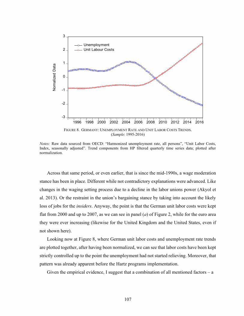
107
-3
-2
-1
0
1
2
3
1996 1998 2000 2002 2004 2006 2008 2010 2012 2014 2016
Unemployment
Unit Labour Costs
No
rna
lize
d D
ata
FIGURE 8. GERMANY: UNEMPLOYMENT RATE AND UNIT LABOR COSTS TRENDS.
(Sample: 1995-2016)
Notes: Raw data sourced from OECD: “Harmonized unemployment rate, all persons”, “Unit Labor Costs,
Index, seasonally adjusted”. Trend components from HP filtered quarterly time series data; plotted after
normalization.
Across that same period, or even earlier, that is since the mid-1990s, a wage moderation
stance has been in place. Different while not contradictory explanations were advanced. Like
changes in the waging setting process due to a decline in the labor unions power (Akyol et
al. 2013). Or the restraint in the union’s bargaining stance by taking into account the likely
loss of jobs for the insiders. Anyway, the point is that the German unit labor costs were kept
flat from 2000 and up to 2007, as we can see in panel (a) of Figure 2, while for the euro area
they were ever increasing (likewise for the United Kingdom and the United States, even if
not shown here).
Looking now at Figure 8, where German unit labor costs and unemployment rate trends
are plotted together, after having been normalized, we can see that labor costs have been kept
strictly controlled up to the point the unemployment had not started relieving. Moreover, that
pattern was already apparent before the Hartz programs implementation.
Given the empirical evidence, I suggest that a combination of all mentioned factors – a

108
-2.0
-1.5
-1.0
-0.5
0.0
0.5
1.0
1.5
2.0
1996 1998 2000 2002 2004 2006 2008 2010 2012 2014 2016
Unemployment
Unit Labour CostsN
orm
ali
zed D
ata
Italy
-2.0
-1.6
-1.2
-0.8
-0.4
0.0
0.4
0.8
1.2
1.6
1996 1998 2000 2002 2004 2006 2008 2010 2012 2014 2016
Unemployment
Unit Labour Costs
Norm
ali
zed D
ata
Spain
-3
-2
-1
0
1
2
1996 1998 2000 2002 2004 2006 2008 2010 2012 2014 2016
Unemployment
Unit Labour Costs
Portugal
Norm
ali
zed D
ata
FIGURE 9. UNEMPLOYMENT RATE AND UNIT LABOR COSTS TRENDS.
(a) ITALY, (b) SPAIN AND (c) PORTUGAL
(Sample: 1995-2016)
Notes: Raw data sourced from OECD: “Harmonized unemployment rate, all persons”, “Unit Labor Costs,
Index, seasonally adjusted”. Trend components from HP filtered quarterly time series data; plotted after
normalization.
cooperative prone culture, changes in labor market institutions, the design and
implementation of new labor policy measures (ALMP) – led to the observed adjustment
process in Germany employment, after the disturbances triggered by the unification and the
world recession in the early 1990s. I further suggest that while being inwardly motivated –
there was no external power imposing structural reforms – that process reflected a high
reflexive institutional endowment.
I tackle now the responses of other euro area members hit by high unemployment
episodes, such as the Peripheral countries. In Figure 9 their unemployment rate and unit labor
costs trends are plotted together, after normalization, to provide a better perspective as
depicted in Figure 8 for Germany. Thereby, we can see that (i) the unit labor costs of Spain
and Portugal clearly adjusted downwards after the 2010-12 European sovereign debt crisis,
but not Italy’s, which kept rising; (ii) unemployment decreased in Spain and Portugal along
with the downward adjustment of the unit labor costs, while was increasing in Italy.
The contrasting evolution of the labor market equilibria after 2010-12 between Portugal
and Spain on the one hand, and Italy on the other hand, should be evaluated in the light of
the conditionality imposed to the former by the financial assistance programs as mentioned
in section 3.1, while Italy was spared from any external interference. A significant package

109
of measures in the adjustment programs focused on the reform of labor market institutions18.
It is worth noting that labor markets were dysfunctional in both Iberian countries. The
Spanish characterized by a high structural rate of unemployment: around 20% in 1995 and
again in 2016, even if the effective rate adjusted downward (8% in 2007) during the booming
years of the euro experiment, when cheap real estate financing inflated the nontradables
output. The Portuguese showing increasing unemployment since the euro inception: from
around 5% in 2000 to 9% in 2007. And both countries evidencing high labor market
segmentation.
We should not ascribe all the credit for the relief in the labor costs to the reforms of the
labor market institutions: Fiscal adjustment and the corresponding downward pressure on
nontradables have for sure played a role. However, there is a remarkable feature in this
process to highlight. As opposed to Germany, where high and persistent unemployment had
led to an endogenously determined regime change in the labor market institutions and
behaviors, the reforms in Spain and Portugal have been exogenously imposed. And in Italy,
a country kept immune from external assistance and the implied structural changes, no
reforms at all were implemented.
There are earlier experiences in Europe of endogenously determined reforms which have
had a significant impact in structural unemployment. Namely, the pro-market transformation
led by Margaret Thatcher in the United Kingdom (Card and Freeman 2004; Siebert 1997)
and the “flexicurity” arrangement in Denmark (Bredgaard et al. 2005; Westergaard-Nielsen
2001). I will not discuss here the specificities of those reforms. They were diverse in scope,
in deepness and in the informing principles, dependent as they were on each country’s social
18 The Economic Adjustment Programme was prepared by the troika consisting of the European Commission,
ECB and IMF, after a request of financial assistance made by Portugal on 7 April 2011. Regarding the labor
market reforms, the stated objectives were to improve flexibility by reducing employment protection, e.g.
excessive severance payments; making wage setting less rigid, e.g. limiting union coverage (in case, by
reviewing the criteria for the extension of collective agreements); to promote job search effort by decreasing
unemployment benefits, which were misaligned with the European averages; make working time
arrangements more flexible and overtime payment less expensive. It should be noticed that employment
protection for permanent contracts in Portugal was the highest among the developed countries in 2011,
accordingly to OEDC classification criteria, “Strictness of employment protection – individual and collective
dismissals (regular contracts), OECD.Stat.
110
infrastructure. High centralized collectively bargained systems work well in more
cooperative society such in the Scandinavia countries19 and Netherlands (Nickell et al. 2000).
Market-based wage setting arrangements are associated with higher employment rates in the
post-Thatcher era in the United Kingdom, for example. What matters here is the reform
proclivity, the reaction or the absence of it to past and ongoing adversarial experiences. In
short, the degree of reflexivity in a given society, and the so-revealed institutional
endowment.
5. THE MISALLOCATION STORY REVISITED
I return now back to the technological shock addressed in section 3.3. An episode of
overvaluation driven by a shift in home demand, such as that one described in section 3.1,
likely harms aggregate productivity growth by diverting resources from the tradables sector
to the less efficient nontradables. However, empirical analysis in the field of growth
accounting, or more specifically in allocative efficiency, has shown that the misallocation of
resources in the Peripheral countries was highly significant within-industry and weighing
much more in the observed TFP deterioration than the between-sector component. This
pattern makes the identification of the mechanics behind the loss in aggregate productivity
much more difficult. I summarize next the main findings on the allocative inefficiency
literature for Italy, Spain and Portugal; and I discuss its possible sources, where the
previously introduced concept of institutional endowment might become useful.
Calligaris et al. (2016) found a substantial increase in misallocation both in manufacturing
and in services since 1995 and have shown that it accounted for a large fraction in the Italian
aggregate TFP slowdown. By applying the Hsieh and Klenow (2009) methodology20, they
estimated that productivity in 2013 would be 18% higher in manufacturing and 67% higher
19 According to Olson (1982, Chapter 4), the fact that Scandinavian countries exhibit a high trade union
density makes the respective unions internalize the impact of their bargaining stance on the overall course of
the economy, including in a long-run perspective (economic growth). This follows from the logic of collective
action theory by which “encompassing organizations” rather than narrow special-interest ones face incentives
to account for the consequences of inefficient policies. 20 In Hsieh and Klenow (2009) methodology, the misallocation of resources is estimated by computing the
dispersion of marginal products of capital and labor across firms.

111
in non-manufacturing if the allocative efficiency prevailing in 1995 had not been degraded.
The analysis was conducted across regions, firm sizes and industries; in any case, the between
misallocation component was small when compared with the within component. It should
be noted that the segment of big firms in the Northwest (i.e., the richest region in Italy)
exhibited the more pronounced increase in misallocation. In 2018, Fadi et al. redid the same
exercise, though being more specific on the more tainted segments, namely the “firms that
have large share of workers under the Italian wage supplementation scheme, that are family
owned, or financially constrained” (p. 4). Furthermore, the authors pointed to “the presence
of sluggish reallocation of resources” as the source of heterogeneity in the ability to respond
to “frontier shocks” (Fadi et al. 2018, p. 4).
In 2017, Pellegrino and Zingales had already taken “frontier shocks”, namely the
Information and Communication Technologies (ICT) revolution21, and its interaction with a
dysfunctional management system, based on loyalty instead of on merit, to explain the
productivity slowdown observed in Italy since the mid-1990. Ultimately, the “institutional
environment” underlined the bias against meritocracy, the authors noted, because “familism
and cronyism” were the most rewarding management attributes to deal with a patronage-
based banking system, an inefficient legal system, the prevalence of tax avoidance and bribes.
Gopinath et al. (2015) analyzed productivity evolution in the manufacturing sector in
Spain between 1999 and 2012 based on a model combining credit frictions and the
framework developed by Hsieh and Klenow (2009). By using a calibrated model, the authors
were able to show the relation between the real interest rate decline since the mid-1990s and
dynamics of the marginal return on capital dispersion and its detrimental effect on the
aggregate TFP evolution. Moreover, they showed a differentiated pattern between countries
in the North and the South of Europe, the latter supposed to represent “less well-developed
financial markets” (p. 4).
García-Santana et al. (2016) extended the misallocation analysis to all sectors in the
Spanish economy, over the period 1995-2007. After employing several measures to compute
allocative efficiency, including again the one proposed by Hsieh and Klenow (2009), they
21 Based on Bresnahan et al. (2002), the authors highlighted that “American firms were able to take advantage
of the Information and Communication Technologies thanks to the meritocratic management practices”, p. 2.

112
found that the within-industry component explained 89% of the decline in TFP over the 1995-
2007 period. The losses in productivity driven by misallocation were more severe in
constructions and services, but even lower also felt in the manufactory sector. However,
differently from Gopinath et al. (2015), they did not found any significant connection with
financial dependence; however, “the deterioration in allocative efficiency was 22.6 points
larger in sectors influenced by regulations” García-Santana et al. (2016, p. 24). It is worth
noting the evidence gathered on the firm size channel of misallocation: The estimate of the
OP covariance term, which capture the relation between size and productivity (Olley and
Pakes 1996), dropped from 0.30 in the observation window 1995-2000 down to 0.21 in
observation window 2001-200722.
Dias et al. (2016), employing the Hsieh and Klenow (2009) methodology, investigated the
misallocation in Portugal over the period 1996-2011 and found that “within-industry
misallocation almost doubled between 1996 and 2011” (p. 48). Moreover, deteriorating
allocative efficiency, which was mostly driven by the service sector, might have “shaved
around 1.3% of annual GDP growth” in that same period (p. 48). Regarding the source of
distortions, a detailed description was presented on economic policies that overprotected and
subsidized SMEs.
In 2011, Braguinsky, Branstetter and Regateiro had already provided a technical
explanation for the bias towards SMEs in Portugal (i.e., against the larger and more efficient
firms) and shown its implication on aggregate productivity. The shift of the firm size
distribution to the left, observed for more than 20 years, was an old rooted problem, stemming
from the prevailing labor market institutions. More specifically, employment protection, for
which Portugal ranked the highest score among the Western European countries. The
framework is based on the Murphy et al. (1991) variation of the seminal work of Lucas (1978)
on firm size distribution. By modeling the costs induced by employment protection as a tax
on labor, T, the so augmented span-of-control model shows that in equilibrium a higher T not
22 For a benchmark, notice that OP covariance term for labour productivity averages 0.51 over 1993-2001 within
the U.S. manufacturing industries. in the US is 0.51 versus 0.20-0.30 for Western European countries
(Bartelsman et al. 2013, pp. 310-11).
113
only leads to smaller sizes of all existing firms but induces entry by entrepreneurs with
relatively lower ability (self-employment included). Hence, the outcome of a leftward shift
of the firm size distribution and the consequent fall in aggregate productivity.
Strict employment protection was also prevalent in Spain and Italy before the euro
adoption. The Spanish labor market was high dysfunctional as revealed by the structural rate
of unemployment (around 20% in 1995). Concerning Italy, the reforms undertaken in the
mid-1990s were more or less restricted to the flexibilization of short-term contracts which
led to a dual labor market and where the old jobs have been kept highly protected (Calligaris
et al. 2016).
Therefore, the three Peripheral countries entered the monetary union exhibiting heavily
taxed employment in the sense of the augmented span-of-control model. I have suggested in
another work more strictly focused on the dismal performance of the Portuguese economy in
the euro23 that, because of the non-linear effects of the “gross tax on labor”24, the impact of
overvaluation on the larger and more efficient enterprises was more than proportional. I argue
that this mechanism stands for the possible link of the euro adoption and the adverse
technological shock observed since the mid-1990s, almost simultaneously, in the three
Peripheral countries.
To sum up, aggregate productivity has taken a symmetric dismal course in Italy, Spain
and Portugal along the process of the euro adoption, which started in the mid-1990s. The
three countries were simultaneously hit by an overvaluation shock while sharing a non-
reflexive “institutional endowment”, where some remarkable features were common (e.g. at
the labor market institutions level) and others more specific (e.g. corporate management and
structure unfitted to the ICT revolution, in Italy). Under the augmented span-of-control model
of Lucas (1978), over-priced wages imply a decrease in the firm optimal size. The empirical
analysis conducted by García-Santana et al. (2016) on Spain offers a perfect illustration on
this point, because, diversely from Italy and Portugal, the Spanish economy boomed in course
of the euro-led financial integration episode. The shift in the demand has not been met by an
23 “Portugal in the Euro, a GVAR approach”. 24 For the non-linear effects of the “gross tax on labor”, see Braguinsky et al. (2011, Section 4.1.2).

114
increase in the production of larger and more efficient firms, but by the smaller and less
efficient enterprises, as shown by the estimated fall in the OP covariance term.
It remains to be said that the explanation based on the interaction of the euro-driven
overvaluation with the firm size distortions, embedded in the “institution endowment”, does
not preclude other shocks or channels. The interaction of the ICT shock with the management
structure in Italy, for example, might have played an overlapping role. Although, two
comments are offered in this respect. First, the ill adaptation to the ICT revolution likely
explains a slower, but not a negative, productivity growth rate. Second, the underlying
distortion is clearly embedded in the Italian institutional framework. Pellegrino and Zingales
(2017), have already suggested that connection. Considering its persistence, this paper
suggests an additional ingredient: the implied low-degree of reflexivity in that same
institutional framework.
6. CONCLUSIONS
Puzzling developments in the euro experiment were the object of inquiry. First, the survival
of the euro area despite not fulfilling the OCA assumptions. Second, the observed diverging
path in the long run where catching up was expected from the integration of the less-
developed economies in more inclusive and advanced institutions.
In what concerns the OCA issue, I suggest that monetary policy might have been
underestimated by the earlier discussions on the adjustment mechanisms in a currency union,
given the still unknown power of the “new-style central banking” (Hall and Reis 2015). For
the gloomy long-run performance of the Peripheral countries addressed in this paper – Italy,
Spain and Portugal –, I emphasize the role of relative prices and institutional frictions.
An episode of overvaluation was observed in the Peripheral countries, starting in the mid-
1990s and going through the European sovereign debt crisis of 2010-12. Why so long? I
suggested an explanation. Diversely from demand shocks propelled by typical financial
integration, this time debt financing was ensured in a shared currency, and the capital inflows
were drawn from a common pool of resources. Thus, the change in relative prices of future

115
to present consumption facing the Periphery had deep foundations. But, how has that episode
of overvaluation hindered economic growth?
Overvaluation, the increase in unit labor cost or the change in the relative price of
nontradables to tradables are interrelated macroeconomic events. The implications over
economic growth when resources are diverted from a more to a less efficient sector are
straightforward. But the story of underperformance in the Periphery was trickier. First, there
was not just the case of a slowdown in aggregate productivity evolution, but even a TFP
negative growth over a long period. Second, the within-industry misallocation of resources
was much higher than the one measured between sectors. Thus, this inquiry pursued with the
following question: Which channel translated the observed overvaluation into the
misallocation of resources within-sectors?
A comparative analysis of the evolution of the labor market institutions (e.g. labor
protection) across a selected group of Western European countries revealed the diversity in
their institutional frameworks. Furthermore, those institutional frameworks were endowed
with different degrees of reflexivity (Giddens 1990) – that is the proclivity to change the rules
after revealed dysfunctionalities.
Overvaluation interplaying with institutional frictions in less-reflexive institutional
endowments diverted the allocation of resources from larger to smaller and less productive
enterprises. This mechanism and its deep foundations solve the intriguing problem of the
long-lasting real impacts of a change in a “mere” monetary framework. In this case, the
connection of the euro introduction and the correlated underperformance in the Periphery.
REFERENCES
Acemoglu, Daron, Simon Johnson, and James Robinson (2005), "The Rise of Europe:
Atlantic Trade, Institutional Change, and Economic Growth", American Economic
Review, 95(3), pp. 546-79.
Acemoglu, Daron, and James Robinson (2012), Why nations fail: The origins of power,
prosperity, and poverty, New York, NY: Crown Publishers (Random House).
Aguiar-Conraria, Luıs, and Maria Joana Soares (2011), "Business Cycle Synchronization
and the Euro: A Wavelet Analysis", Journal of Macroeconomics, 33(3), pp. 477-89.
116
Ahlborn, Markus, and Marcus Wortmann (2018), "The core‒periphery pattern of European
business cycles: A fuzzy clustering approach", Journal of Macroeconomics, 55, pp.
12-27.
Akyol, Metin, Michael Neugart, and Stefan Pichler (2013), "Were the Hartz reforms
responsible for the improved performance of the German labour market?",
Economic Affairs, 33(1), pp. 34-47.
Altavilla, Carlo, Domenico Giannone, and Michele Lenza (2014), "The financial and
macroeconomic effects of OMT announcements", European Central Bank (ECB)
Working Paper 1707.
Aoki, Kosuke, Gianluca Benigno, and Nobuhiro Kiyotaki (2010), "Adjusting to capital
account liberalization", CEPR Discussion Paper 1014.
Bartelsman, Eric, John Haltiwanger, and Stefano Scarpetta (2013), "Cross-country
differences in productivity: The role of allocation and selection", American
Economic Review, 103(1), pp. 305-34.
Bayoumi, by Tamim, and Barry Eichengreen (2018), "Aftershocks of Monetary
Unification: Hysteresis with a Financial Twist", Journal of Banking and Finance,
Available online 19 June 2018, Article 105365, pp. -.
Bayoumi, Tamim, and Barry Eichengreen (1992), "Shocking aspects of European monetary
unification", National Bureau of Economic Research Working Paper 3949.
Blanchard, Olivier (2006), "European unemployment: the evolution of facts and ideas",
Economic Policy, 21(45), pp. 5-59.
Blanchard, Olivier Jean, and Lawrence F. Katz (1992), "Regional evolutions", Brookings
Papers on Economic Activity, 1992(1), pp. 1-75.
Braguinsky, Serguey, Lee G Branstetter, and Andre Regateiro (2011), "The Incredible
Shrinking Portuguese Firm", National Bureau of Economic Research Working
Paper 17265.
Bredgaard, Thomas, Flemming Larsen, and Per Kongshøj Madsen (2005), "The flexible
Danish labour market–a review", Aalborg University, Centre for Labour Market
Research (CARMA) Research paper 2005:1.
Bresnahan, Timothy F, Erik Brynjolfsson, and Lorin M Hitt (2002), "Information
technology, workplace organization, and the demand for skilled labor: Firm-level
evidence", Quarterly Journal of Economics, 117(1), pp. 339-76.
Brunnermeier, Markus K, Harold James, and Jean-Pierre Landau (2016), The Euro and the
Battle of Ideas, Princeton, NJ: Princeton University Press.
Calligaris, Sara, Massimo Del Gatto, Fadi Hassan, Gianmarco IP Ottaviano, and Fabiano
Schivardi (2016), "A Study on Resource Misallocion in Italy", European Comunity
Discussion Paper 030/2016.

117
Calvo, Guillermo A. (1998), "CAPITAL FLOWS AND CAPITAL-MARKET CRISES:
The Simple Economics of Sudden Stops", Journal of Applied Economics, 1(1), pp.
35.
Campos, Nauro F., and Corrado Macchiarelli (2016), "Core and Periphery in the European
Monetary Union: Bayoumi and Eichengreen 25 years later", Economics Letters,
147, pp. 127-30.
Card, David, and Richard B Freeman (2004), "What have two decades of British economic
reform delivered?," in Seeking a Premier Economy: The Economic Effects of British
Economic Reforms, 1980-2000, edited by David Card, Richard Blundell, and
Richard B. Freeman, pp. 9-62: University of Chicago Press.
Caselli, Francesco (2005), "Accounting for Cross-Country Income Differences," in
Handbook of Economic Growth, edited by Aghion Philippe and N. Durlauf Steven,
pp. 679-741: Elsevier.
De Grauwe, Paul (2013), "The European Central Bank as Lender of Last Resort in the
Government Bond Markets", CESifo Economic Studies, 59(3), pp. 520-35.
De Haan, Jakob, Robert Inklaar, and Richard Jong‐A‐Pin (2008), "Will business cycles in
the euro area converge? A critical survey of empirical research", Journal of
Economic Surveys, 22(2), pp. 234-73.
Dias, Daniel A., Carlos Robalo Marques, and Christine Richmond (2016), "Misallocation
and productivity in the lead up to the Eurozone crisis", Journal of Macroeconomics,
49, pp. 46-70.
Fadi, Sara Calligaris Massimo Del Gatto, Gianmarco IP Hassanz, Sara Calligaris, Massimo
Del Gatto, Fadi Hassanz, and Gianmarco IP Ottaviano (2018), "The Productivity
Puzzle and Misallocation: an Italian Perspective", Luiss Lab of European
Economics LLEE Working Paper 142.
Fagan, Gabriel, and Vitor Gaspar (2007), "Adjusting to the Euro", European Central Bank
(ECB) Working Paper 716.
Falagiarda, Matteo, and Stefan Reitz (2015), "Announcements of ECB unconventional
programs: Implications for the sovereign spreads of stressed euro area countries",
Journal of International Money and Finance, 53, pp. 276-95.
Feyrer, James, and Bruce Sacerdote (2013), "How Much Would US Style Fiscal Integration
Buffer European Unemployment and Income Shocks? (A Comparative Empirical
Analysis)", American Economic Review, 103(3), pp. 125-28.
Friedman, Milton (1953), "The Case for Flexible Exchange Rates," in Essays in positive
economics, pp. 157-203, Chicago: University of Chicago Press.
— (1997, August 28), "The Euro: Monetary Unity to Political Disunity", Project Syndicate.
Friedman, Milton, and Anna Jacobson Schwartz (1963), A Monetary History of the United
States, 1867-1960, 9th paperback ed. (1993). Princeton, NJ: Princeton University
Press.
118
García-Santana, M, E Moral-Benito, J Pijoan-Mas, and R Ramos (2016), "Growing like
Spain: 1995-2000", Banco de Espana Working Paper 1609.
Giavazzi, Francesco, and Luigi Spaventa (2010), "Why the Current Account Matters in a
monetary Union: Lessons from the Financial Crisis in the Euro Area", CEPR
Discussion Papers 8008.
Giddens, Anthony (1990), The consequences of modernity, Cambridge UK: Polity Press.
Goodhart, C. A. E., and D. J. Lee (2013), "Adjustment Mechanisms in a Currency Area",
OPEN ECONOMIES REVIEW, 24(4), pp. 627-56.
Gopinath, Gita, Sebnem Kalemli-Ozcan, Loukas Karabarbounis, and Carolina Villegas-
Sanchez (2015), "Capital Allocation and Productivity in South Europe", National
Bureau of Economic Research Working Paper 21453.
Hall, Robert E, and Charles I Jones (1999), "Why do some countries produce so much more
output per worker than others?", Quarterly Journal of Economics, 114(1), pp. 83-
116.
Hall, Robert E., and Ricardo Reis (2015), "Maintaining Central-Bank Financial Stability
under New-Style Central Banking", National Bureau of Economic Research
Working Paper 21173.
Hodrick, Robert J, and Edward C Prescott (1997), "Postwar US business cycles: an
empirical investigation", Journal of Money, Credit, and Banking, pp. 1-16.
Hsieh, Chang-Tai, and Peter J Klenow (2009), "Misallocation and Manufacturing TFP in
China and India", Quarterly Journal of Economics, 124(4), pp. 1403-48.
— (2010), "Development Accounting", American Economic Journal: Macroeconomics,
2(1), pp. 207-23.
Judt, Tony (2011), A grand illusion?: an essay on Europe, New York, NY: NYU Press.
Kang, Joong Shik, and Jay C. Shambaugh (2016), "The rise and fall of European current
account deficits", Economic Policy, 31(85), pp. 153-99.
Kenen, P (1969), "The theory of optimum currency areas," in Monetary Problems of the
International Economy, edited by R. Mundell and A. Swoboda, pp. 41–60 Chicago:
University of Chicago Press.
Klein, Michael W, and Jay C Shambaugh (2012), Exchange rate regimes in the modern
era, Cambridge, MA: MIT Press.
Krugman, Paul (2013), "Revenge of the optimum currency area", NBER macroeconomics
annual, 27(1), pp. 439-48.
Lane, Philip R (2012), "The European sovereign debt crisis", The Journal of Economic
Perspectives, 26(3), pp. 49-67.
Lucas, Robert E (1978), "On the Size Distribution of Business Firms", The Bell Journal of
Economics, 9(2), pp. 508-23.
119
McCloskey, Deirdre N (2016), Bourgeois equality: How ideas, not capital or institutions,
enriched the world, Chicago and London: University of Chicago Press.
Merler, Silvia, and Jean Pisani-Ferry (2012), "Sudden stops in the euro area", Bruegel
Policy Contribution 2012/06.
Mundell, Robert (1998, March 24), "The Case for the Euro—I", Wall Street Journal.
Mundell, Robert A (1961), "A theory of optimum currency areas", American Economic
Review, 51(4), pp. 657-65.
Murphy, Kevin M, Andrei Shleifer, and Robert W Vishny (1991), "The Allocation of
Talent: Implications for Growth", Quarterly Journal of Economics, 106(2), pp. 503-
30.
Neal, Larry (1993), The rise of financial capitalism: International capital markets in the
age of reason, Cambridge, UK: Cambridge University Press.
Nickell, Steve, Jan Van Ours, and Harry Huizinga (2000), "The Netherlands and the United
Kingdom: a European unemployment miracle?", Economic Policy, 15(30), pp. 137-
80.
North, Douglass C (1990), Institutions, institutional change and economic performance,
Cambridge, UK: Cambridge University Press.
— (2006), Understanding the process of economic change, Princeton, NJ: Princeton
University Press.
North, Douglass C, and Robert Paul Thomas (1973), The rise of the western world: A new
economic history, Cambridge, UK: Cambridge University Press.
North, Douglass C, and Barry R Weingast (1989), "Constitutions and commitment: the
evolution of institutions governing public choice in seventeenth-century England",
The Journal of Economic History, 49(04), pp. 803-32.
Olley, G Steven, and Ariel Pakes (1996), "THE DYNAMICS OF PRODUCTIVITY IN
THE TELECOMMUNICATIONS EQUIPMENT INDUSTRY", Econometrica,
64(6), pp. 1263-97.
Olson, Mancur (1982), The rise and decline of nations: Economic growth, stagnation, and
social rigidities, New Heaven, CT: Yale University Press.
Pellegrino, Bruno, and Luigi Zingales (2017), "Diagnosing the Italian disease", National
Bureau of Economic Research Working Paper 23964.
Pissarides, Christopher A (2013), "Unemployment in the great recession", Economica,
80(319), pp. 385-403.
Rebelo, Sergio, and Carlos A Vegh (1995), "Real effects of exchange-rate-based
stabilization: an analysis of competing theories", NBER macroeconomics annual,
10, pp. 125-74.
Reis, Ricardo (2013), "The Portuguese Slump and Crash and the Euro-Crisis", Brookings
Papers on Economic Activity, Spring, pp. 143-93.

120
Rinne, Ulf, and Klaus F Zimmermann (2013), "Is Germany the North Star of Labor Market
Policy?", IMF Economic Review, 61(4), pp. 702-29.
Sala-i-Martin, Xavier, and Jeffrey Sachs (1991), "Fiscal federalism and optimum currency
areas: evidence for Europe from the United States", National Bureau of Economic
Research Working Paper 3855.
Schmitt-Groh, Stephanie, and Martín Uribe (2013), "Downward Nominal Wage Rigidity
and the Case for Temporary Inflation in the Eurozone", Journal of Economic
Perspectives, 27(3), pp. 193-212.
Shambaugh, Jay C. (2012), "The Euro's Three Crises", Brookings Papers on Economic
Activity, Spring, pp. 157-231.
Siebert, Horst (1997), "Labor Market Rigidities: At the Root of Unemployment in Europe",
Journal of Economic Perspectives, 11(3), pp. 37-54.
Svirydzenka, Katsiaryna (2016), "Introducing a New Broad-based Index of Financial
Development", International Monetary Fund IMF Working Paper 16/5.
Szczerbowicz, Urszula (2015), "The ECB Unconventional Monetary Policies: Have They
Lowered Market Borrowing Costs for Banks and Governments?", International
Journal of Central Banking, 11(4), pp. 91-127.
Tirole, Jean (2006), The Theory of Corporate Finance, Princeton, NJ: Princeton University
Press.
Weber, Max (1904-1905), The Protestant Ethic and the Spirit of Capitalism (Die
Protestantische Ethik und der Geist des Kapitalismus), (1958). Translated by
Talcott Parsons (1930), from 1920 German Edition. New York, NY: Scribner's.
Westergaard-Nielsen, Niels (2001), "Danish Labor Market Policy: Is it Worth it?", Aalborg
University, CLS Working Paper 01-10.
Williamson, Oliver E (1985), The Economic Institutions of Capitalism, New York, NY:
Free Press.
Wunsch, Conny (2005), "Labour market policy in Germany: institutions, instruments and
reforms since unification", Universitat St Gallen Economics Discussion Paper 2005-
06.

ESSAY NO. 3
Dynamical Analysis of the Euro Area Using Oil Shocks
– A GVAR Approach*
Abstract
We return to oil shocks to study the evolution of the economic
structures among the euro area member states as the euro
experiment moves ahead. Are oil shocks still a meaningful
conceptual experiment despite the Great Moderation and the
prevalence of oil demand shocks in the last two decades? By
modeling oil prices as a “dominant unit” in a GVAR framework, this
paper restates its usefulness to conduct dynamic analysis. Both the
positive initial impact of oil price surges driven by global demand
and the lagged adverse effects on the output of net energy importers
are captured. Noticeably for Germany, which output responses to
global shocks further, and surprisingly, show to be more aligned with
the Periphery rather than with the Core. Meanwhile, the Peripheral
economies became less heterogeneous; although, the evidence for
closer resemblance with the Core is mixed. Finally, the empirical
results point to a persistent sluggish adjustment of inflation in the
Periphery.
Keywords: Euro area, Germany, Global VAR, Oil shocks.
JEL Codes: C51, E32, F45, F47
*This is a joint work with my PhD co-supervisor, Professor Luís Aguiar-Conraria, who has suggested using
oil shocks and the GVAR methodology to study the evolution of the euro area economic structure across
its members.

122
1. INTRODUCTION
The euro area has completed 20 years since its inception, viz. the irrevocable fixing of
the exchanges rates for the eleven initial members on 1 January 1999. For the Peripheral
countries, the movement towards financial integration had started even earlier, in the mid-
1990s. Thus, it seems pertinent to question if the fundamentals for the adoption of a
common currency have strengthened in the meanwhile.
Measuring business cycle synchronization is a well-known method to address the
problem, but the findings in that strand of the literature are ambiguous or even
contradictory. In a critical review of the empirical research, De Haan et al. (2008), for
example, concluded that there was no evidence of convergence of business cycles across
the euro area countries. More recent studies present mixed results: either against the
convergence towards a “European business cycle” (Ahlborn and Wortmann 2018) or
“only a limited support” in that direction (Bayoumi and Eichengreen 2018); or showing
increasing business cycle synchronization after the euro introduction (Aguiar-Conraria et
al. 2013; Campos et al. 2019).
The matter of concern is the optimality of a single monetary policy, which imply the
stabilization of both output fluctuations and inflation. Therefore, we restate the
synchronicity problem in the following terms: Did the economic structures of the euro
area countries converge as the euro experiment advanced?
We suggest that the economic structure must be taken in a broader sense when
discussing the membership in a currency area. In common usage, it refers to “regional
specialization” (Krugman 2001). We further consider the institutional framework. If the
labor market institutions, for example, were similar across the members of a currency
union, the effects of an adverse supply shock on employment, or the output gap, would
fall apart less. The same might be said about the impact on inflation of a positive demand
shock.
By using oil shocks – a common global variable – we can disturb both variables of
interest, the real output and inflation and compare the country-specific responses. Hence,
this paper employs oil shocks as the “conceptual experiment” 1 to test the economic
1 We borrowed the “conceptual experiment” expression from Koop et al. (1996) in the context of impulse
response analysis.

123
structures of the euro area countries.
This is not new of course. In 2009, Peersman and Van Robays already employed oil
shocks to investigate asymmetries across the euro area members. Although our
contribution is distinctive in two fundamental aspects. First, using a different
methodology, namely the global VAR (GVAR). Second, by seeking to evaluate the
convergence in the behavior of the variables of interest as the euro experiment moves
ahead.
But again, using the GVAR2 to study the euro area is not new in the literature. The
empirical model adopted in the present work is based on a version built by Dees et al.
(2007) precisely for “Exploring the international linkages of the euro area”. However,
whereas the euro area was then taken as a single region, this paper addresses each member
country individually, as well as the aggregates for the euro-area Core and the euro-area
Periphery regions. Furthermore, the price of oil was included by Dees et al. (2007) in the
list of the endogenous variables of the U.S. “conditional model”3. Here we make use of
an alternative specification where oil prices are defined as a “dominant variable” in a
sense later advanced by Chudik and Pesaran (2013). Accordingly, in this paper, the oil
prices are framed in a “marginal model" and enter as weak exogenous in the U.S. model,
likewise in all countries in the sample. This option entails a remarkable distinction when
conducting the impulse response analysis. A positive shock to oil prices entertained in a
“marginal model" means a rise in the price of oil. That same shock is a mere disturbance
of the error term of the oil price equation in the U.S. model when oil prices are framed in
a “conditional” model.
All euro area members are net energy importers. Therefore, as argued by Blanchard
and Gali (2007), a rise in oil prices, even when driven by a shift in global demand, turns
into an exogenous adverse shock to those economies. However, we should not disregard
that an “oil demand shock” (Kilian 2009), whereby conveying the signal of an increase
in global demand, might prompt different responses across the European economies. See,
for example, the case of Germany and Portugal, where the former exports to the large
emerging and transition economies, notably China, while the latter is exposed to its
2 Chudik and Pesaran (2016) offer a concise description of the GVAR methodology and a review of the
empirical work undertaken since its introduction by Pesaran et al. (2004). 3 See, for example, Garratt et al. (2006, pp. 58-9) for the definition of “conditional” and “marginal”
models.

124
competition on less advanced manufactured products (e.g., textiles). By modeling the oil
shocks as a “dominant unit” in the GVAR framework, the adverse impact of an increase
in oil prices on energy-importing countries is captured without missing the possible
favorable comovements between the domestic GDP and its foreign counterparts. On one
hand, the adverse exogenous effects a la Blanchard and Gali (2007) are identified by the
direct “causal nature of the common variable” (Chudik and Pesaran 2016, p. 170 ). On
the other hand, the positive effects of an oil demand shock a la Kilian (2009) is “integrated
out” throughout the properties of the generalized impulse response functions (GIRFs)4
adopted by the GVAR methodology. Subsection 3.2 and Appendix B provide the
technical details.
That said, the evolution of the composition of oil shocks over our sample period,
1979Q2-2016Q4, become relevant to interpret the results of the empirical analysis. The
same is true for the changing patterns on the interaction of oil shocks with the
macroeconomic variables of interest since the mid-1980s, that is along the “Great
Moderation”. Therefore, when defining the observation windows to tackle the evolution
of the economic structure of the euro area countries, we take into account those structural
changes. Therefore, the year 1986, which was identified as a break date in the oil literature
(Baumeister and Peersman 2013), was chosen as the splitting mark. Hence, we define the
first observation window (W1) throughout 1979Q2-2010Q1 and the second observation
window (W2) throughout 1986Q1-2016Q4. Each one assembles the same number of
observations, 151 quarters. An overlapping time span was unavoidable for conducting
meaningful impulse response analysis.
The second observation window offers the best context to evaluate the methodology
adopted in this paper. As the basic facts reported in section 2 show, “oil demand shocks”
episodes were prevalent in that period. Even though their impacts on the output of larger
and open economies, including the euro area countries, are statistically significant, sizable
and negative, around the 12th quarter. Therefore, the results of the dynamic analysis
conducted with the GVAR version adopted in our study fits the prevision of Blanchard
and Gali (2007) – oil shocks, even when driven by global demand, turns into an
exogenous adverse shock for net energy importers countries.
4 We owe the GIRFs to Koop et al. (1996) and its application in vector error-correcting models to Pesaran
and Shin (1998).

125
Therefore, the adopted framework – oil prices modeled as a “dominant variable” in a
GVAR model – reveals an appropriate tool to investigate the evolution of the economic
structure of the euro area members. Notably for Germany, which was the European
economy that has most benefited from the heightening of the oil-demand accent in the
composition of oil shocks. Even though the statistical significance of its real GDP impulse
responses slightly improved when we move from observation window W1 to observation
window W2. This feature underlies what might be the most distinctive contribution of the
present paper. Germany exhibits in the euro area, along with Portugal, the most
impressive shift towards convergence in output fluctuations, when evaluated by the
response to global shocks.
The remainder of this paper is organized as follows. Section 2 reports basic data
tracking oil shocks episodes and possible related patterns of “regional specialization”
across the euro area. Section 3 presents the empirical model specification, the criteria to
define the observation windows and the data sources. Section 4 portrays and discuss the
results of the dynamical analysis (GIRFs) for two focus groups. The first group comprises
the large/open economies, including the United States, the euro-area Core and the euro-
area Periphery regions. The second group comprehend eleven initial euro area members,
plus Denmark. Section 5 concludes.
2. BASIC FACTS
Two basic facts seem of interest before undertaking the empirical analysis of the euro
area dynamics using oil price shocks. First, the evolution of oil prices and its underlying
drivers, that is the global demand and oil production, throughout the sample period of
1979Q2-2016Q4. Second, patterns in the economic structure of the euro area members
possible leading to different responses to oil shocks of distinct composition.
2.1 Oil Shocks Episodes
Figure 1 displays basic data to tackle the first issue, by plotting the (log) real price of oil
over 1979Q2-2016Q4, the (log) oil production, and an indicator of “economic activity”5,
5 Monthly raw data for the three selected time series (real oil price; oil production and real “economic
activity”) were retrieved from https://sites.google.com/site/cjsbaumeister/research, on 14 May 2019.

126
3.8
4.0
4.2
4.4
4.6
4.8
5.0
2.0
2.5
3.0
3.5
4.0
4.5
1980 1985 1990 1995 2000 2005 2010 2015
Economic Activity Oil Production Real Oil Price
Eco
no
mic
Act
ivit
y a
nd
Oil
Pro
du
ctio
n
Real O
il Price
FIGURE 1. OIL PRICE SHOCKS EPISODES
DARK SHADED AREAS: SUPPLY-DRIVEN SHOCKS; LIGHT SHADED AREAS: DEMAND-DRIVEN SHOCKS.
Notes: Data Sources: The raw data for the real oil prices, oil production and real economic activity
(OECD+6NME industrial production) are from the Baumeister and Hamilton (2019) dataset. The
identification of the oil shocks episodes, and its discrimination among demand-driven or supply-driven
shocks, are based on the works of Blanchard and Gali (2007), Hamilton (2009), and Baumeister and
Hamilton (2019).
again in real terms and logs; plus, the observed oil shocks episodes, marked by the shaded
areas. “Economic activity”, proxying global demand, is measured by an “extended
version of the OECD’s index of monthly industrial production in the OECD and six major
other countries [Brazil, China, India, Indonesia, the Russian Federation and South
Africa]”, as proposed by Baumeister and Hamilton (2019, p. 1891). The oil shocks
episodes are traced by combining insights from the works of Blanchard and Gali (2007),
Hamilton (2009), and Baumeister and Hamilton (2019).
We start by offering some comments on the behavior of the price of oil. From now
on, we assume 1986Q1 as a turning point in oil price dynamics and its macroeconomic
implications, likewise in Peersman and Van Robays (2009). In so doing, we bear in mind
both the “Great Moderation”, that is the decline in the U.S. output fluctuations since the
mid-1980s (McConnell and Perez-Quiros 2000); and the fall in the short-run price

127
elasticity of oil demand, where 1986Q1 was identified as a break date by a Baumeister
and Peersman (2013).
Accordingly, we can see a drop of about 53% in the average real price of oil after
1986, after taking the average of the (log) real price of oil over 1979Q2-1985Q4, which
amounts to 3.51, and compare with the average in the period 1986Q1-2016Q4, which
amounts to 2.98. On the other hand, and after computing standard deviations in both
subperiods, 0.20 in 1979Q2-1985Q4 versus 0.36 in 1986Q1-2016Q4, we can see that the
volatility of oil prices augmented after 1986, which is in accordance with the above-noted
decrease in the price elasticity of oil demand.
We look now at the evolution of demand and supply for oil in the global market (i.e.,
the real “economic activity”) and oil production time series plotted in Figure 1. From
1979Q2 through 2016Q4, the “economic activity” almost doubled in real terms (a rise of
96%), whereas the quantity of oil produced augmented only 26%. Thus, the data hints the
long-run decline in energy intensity, which has been pointed out as one factor, among
others’, behind the dampening of the output responses to oil shocks (Blanchard and Gali
2007).
Finally, we address the oil price shocks episodes. Dark gray shaded areas in Figure 1
denote oil price surges driven by supply disruptions, whereas light gray shaded areas
indicate oil price surges driven by global demand. The 1978-79 episode is related with
the “Iranian revolution in the fall of 1978”, the 1980-81 with “Iraq’s invasion of Iran in
September 1980” and the 1990-91 with “Iraq’s invasion of Kuwait in August 19906”
(Hamilton 2009, p. 220). We follow Blanchard and Gali (2007) when marking the
intervals 1999Q1-2000Q4 and 2002Q1-2005Q3 as large oil shock episodes. And given
that global demand and the supply of oil were both moving up (see the paths of “economic
activity” and “oil production” shown in Figure 1), we have ascribed those episodes to the
category of oil demand shocks7. Finally, there are the 2007-08 and 2016 oil demand
6 For Kilian (2009, p. 1063), “the sharp spike in the real price of oil in 1990-1991 after the invasion of
Kuwait is almost entirely due to an increase in precautionary demand”. As such, it is an episode that lays
in the class of an “oil-specific demand shock” instead of an “oil supply shock”. In turn, Blanchard and
Gali (2007, p. 10) have downplayed this episode given that it did not meet the defined criteria, where a
large oil shock is “an episode involving a cumulative change in the (log) price of oil above 50%,
sustained for more than four quarters”. 7 For (Kilian 2009, p. 1064) , “The sharp rise in the real price of oil in 1999-2000” was driven "again by
factors specific demand for crude oil.”
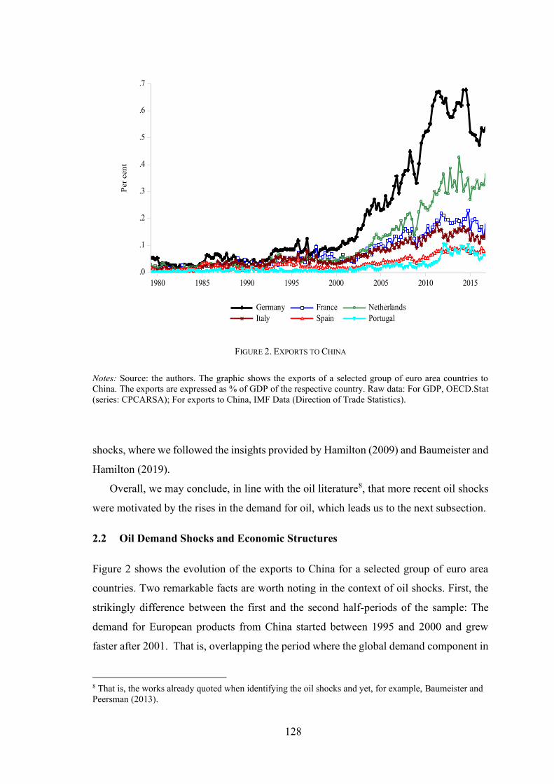
128
FIGURE 2. EXPORTS TO CHINA
Notes: Source: the authors. The graphic shows the exports of a selected group of euro area countries to
China. The exports are expressed as % of GDP of the respective country. Raw data: For GDP, OECD.Stat
(series: CPCARSA); For exports to China, IMF Data (Direction of Trade Statistics).
shocks, where we followed the insights provided by Hamilton (2009) and Baumeister and
Hamilton (2019).
Overall, we may conclude, in line with the oil literature8, that more recent oil shocks
were motivated by the rises in the demand for oil, which leads us to the next subsection.
2.2 Oil Demand Shocks and Economic Structures
Figure 2 shows the evolution of the exports to China for a selected group of euro area
countries. Two remarkable facts are worth noting in the context of oil shocks. First, the
strikingly difference between the first and the second half-periods of the sample: The
demand for European products from China started between 1995 and 2000 and grew
faster after 2001. That is, overlapping the period where the global demand component in
8 That is, the works already quoted when identifying the oil shocks and yet, for example, Baumeister and
Peersman (2013).
.0
.1
.2
.3
.4
.5
.6
.7
1980 1985 1990 1995 2000 2005 2010 2015
Germany France Netherlands
Italy Spain Portugal
Per
cen
t

129
oil shocks became predominant. Second, the dynamics of German exports in contrast with
the almost inexpressive weight of the exports to China from the Iberian countries (Spain
and Portugal).
Thus, the oil price series over the sample period of 1979Q2-2016Q4 contains varying
patterns which likely make the shocks entertained to that “common global variable” a
valuable experiment to study the macroeconomic dynamics of the euro area countries.
3. THE EMPIRICAL MODEL
The matter of concern is the dissimilarities in the economic structure among the members
of a currency union – the euro area, in case – leading to different behaviors on the
macroeconomic variables relevant for conducting (a single) monetary policy.
Hence, the justification for including the real output and inflation in the list of
variables of our empirical model is immediate. But before going further, let us make clear
the definition of economic structure. In common usage, its scope is restricted to patterns
of “regional specialization”. See, for example, Krugman (2001), when discussing the
optimality of currency areas. That might be enough, we suggest, when the interest lies
on output aggregates, either its cyclical fluctuations or the asymmetric responses to global
shocks – the latter stemming from patterns of industrial specialization such as those
evidenced by the exports to China from Germany and Portugal (see subsection 2.2).
However, tackling inflation is not a minor issue in this context. Recall that, in its formal
definition, “The primary objective of the ECB’s monetary policy is to maintain price
stability”9; and we also should bear in mind the trade-offs between the output gap and the
stabilization of inflation. That said, the underlying structural features that make price
adjustments smoother or sluggish are relevant when approaching the fundaments of a
currency union. In particular, wage rigidities, as highlighted by Blanchard and Gali
(2007) in the context of oil shocks analysis, and that prevail in different degrees across
the European countries (see Blanchard 2006).
The purpose of this paper is not going through the analysis of those matters. But we
should bear in mind the underlying heterogeneities across the euro area countries.
Therefore, we take the economic structure, from now on, in a broader sense, subsuming
9 < https://www.ecb.europa.eu/mopo/intro/html/index.en.html>, accessed on 10 June 2019.
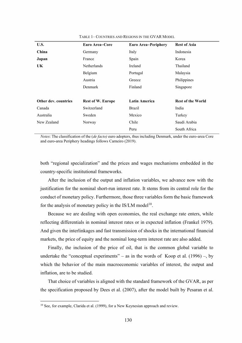
130
TABLE 1– COUNTRIES AND REGIONS IN THE GVAR MODEL
U.S. Euro Area−Core Euro Area−Periphery Rest of Asia
China Germany Italy Indonesia
Japan France Spain Korea
UK Netherlands Ireland Thailand
Belgium Portugal Malaysia
Austria Greece Philippines
Denmark Finland Singapore
Other dev. countries Rest of W. Europe Latin America Rest of the World
Canada Switzerland Brazil India
Australia Sweden Mexico Turkey
New Zealand Norway Chile Saudi Arabia
Peru South Africa
Notes: The classification of the (de facto) euro adopters, thus including Denmark, under the euro-area Core
and euro-area Periphery headings follows Carneiro (2019).
both “regional specialization” and the prices and wages mechanisms embedded in the
country-specific institutional frameworks.
After the inclusion of the output and inflation variables, we advance now with the
justification for the nominal short-run interest rate. It stems from its central role for the
conduct of monetary policy. Furthermore, those three variables form the basic framework
for the analysis of monetary policy in the IS/LM model10.
Because we are dealing with open economies, the real exchange rate enters, while
reflecting differentials in nominal interest rates or in expected inflation (Frankel 1979).
And given the interlinkages and fast transmission of shocks in the international financial
markets, the price of equity and the nominal long-term interest rate are also added.
Finally, the inclusion of the price of oil, that is the common global variable to
undertake the “conceptual experiments” – as in the words of Koop et al. (1996) –, by
which the behavior of the main macroeconomic variables of interest, the output and
inflation, are to be studied.
That choice of variables is aligned with the standard framework of the GVAR, as per
the specification proposed by Dees et al. (2007), after the model built by Pesaran et al.
10 See, for example, Clarida et al. (1999), for a New Keynesian approach and review.

131
(2004). Although, we take the alternative of modeling the oil prices in a dominant unit,
instead of including in the list of endogenous variables of the U.S. country model – a
choice to be highlighted and justified ahead, in the subsection 3.2.
The sample geographic coverage, comprising 36 countries and representing around
90% of the world output, is roughly the same as in Dees et al. (2007). However, we added
Denmark, Greece, Ireland, Portugal, and excluded Argentina for data limitations. Table
1 shows the full list of countries in the sample, and where the euro adopters are organized
under the headings “euro-area Core” and “euro-area Periphery”, following the criteria
presented by Carneiro (2019).
3.1 The Model Specification
In the specification of the variables, we follow Dees et al. (2007). Thus, the endogenous
variables are the (log) real GDP, 𝑦𝑖𝑡, the inflation rate, 𝜋𝑖𝑡, the (log) real equity prices,
𝑒𝑞𝑖𝑡, the (log) real exchange rate, 𝑒𝑖𝑡 − 𝑝𝑖𝑡, the nominal short-term interest rate, 𝑟𝑖𝑡, and
the long-term interest rate, 𝑙𝑟𝑖𝑡11. Although, in the real GDP definition we normalize the
real GDP index by the country population, making 𝑦𝑖𝑡 = 𝑙𝑛( 𝑟𝑒𝑎𝑙 𝐺𝐷𝑃𝑖𝑡) − 𝑙𝑛( 𝑃𝑜𝑝𝑖𝑡/
𝑃𝑜𝑝𝑖̅̅ ̅̅ ̅̅ ), and where 𝑃𝑜𝑝𝑖𝑡 states for the population of country i in quarter t= 1,…, 151, and
𝑃𝑜𝑝𝑖̅̅ ̅̅ ̅̅ is the mean of country I population over the full sample period, 1979Q2-2016Q4.
Hence, we follow the criteria adopted by Carneiro (2019) to get the output data rid of
variations stemming from population growth at different rates across countries in a
lengthy sample period.12
The price of oil is taken as a (dominant) common global variable 𝑝𝑡𝑜 = 𝑙𝑛( 𝑃𝑂𝐼𝐿𝑡),
where 𝑃𝑂𝐼𝐿𝑡 is the price of oil in USD. It deserves to be noticed that the null hypotheses
of weak exogeneity of oil prices is rejected only for three countries (the Netherlands,
Norway and Peru) in observation window W1, spanning over 1979Q2-2010Q1; and is
rejected only for one country (Malaysia) in observation window W2, spanning over
1986Q1-2016Q4.
11 Interest rates are defined in a quarterly basis, e.g., 𝑟𝑖𝑡 = 0,25 × 𝑙𝑛( 1 + 𝑅𝑖𝑡
𝑆 /100), where 𝑅𝑖𝑡𝑆 is the
nominal short-term rate of interest per annum, in percent. 12 We may pick an elucidative example even restricting the sample to the developed economies: The
cumulative growth of the U.S. population was of 45% over 1979-2016, while only 7% for the UK and
10% for Japan.

132
TABLE 2–VARX* MODEL SPECIFICATION
Variables U.S. model Other countries model
Domestic Foreign Domestic Foreign
Real output 𝑦𝑈𝑆,𝑡 𝑦𝑈𝑆,𝑡∗ 𝑦𝑖𝑡 𝑦𝑖𝑡
∗
Inflation 𝜋𝑈𝑆,𝑡 𝜋𝑈𝑆,𝑡∗ 𝜋𝑖𝑡 𝜋𝑖𝑡
∗
Real equity price 𝑒𝑞𝑈𝑆,𝑡 – 𝑒𝑞𝑖𝑡 𝑒𝑞𝑖𝑡∗
Real exchange rate – 𝑒𝑈𝑆,𝑡∗ − 𝑝𝑈𝑆,𝑡
∗ 𝑒𝑖𝑡 − 𝑝𝑖𝑡 –
Nominal short-term interest rate 𝑟𝑈𝑆,𝑡 – 𝑟𝑖𝑡 𝑟𝑖𝑡∗
Nominal long-term interest rate 𝑙𝑟𝑈𝑆,𝑡 – 𝑙𝑟𝑖𝑡 𝑙𝑟𝑖𝑡∗
Oil prices (DU) – 𝑝𝑡𝑜 – 𝑝𝑡
𝑜
Notes: “Other countries model”: A domestic variable will not enter a specific country model in case of missing
observations. Thus, and in what concerns the euro adopters, the price of equity is not included in the models of
Greece, Ireland and Portugal; the short-term interest rate is not included in Denmark; and the long-term interest
rate is not included in Denmark, Finland and Greece.
Finally, in the construction of the star variables, that is, the weighted foreign-countries
counterparts, 𝑦𝑖𝑡∗ , 𝜋𝑖𝑡
∗ , 𝑒𝑞𝑖𝑡∗ , 𝑟𝑖𝑡
∗ , 𝑙𝑟𝑖𝑡∗ , we have used the trade weights, averaged over the
full sample period.
Table 2 summarizes the country-specific VARX* models as per the described choice
of variables13. The models are the same for all countries with exception to the United
States, which is assumed as the numeraire or “reference country” (Pesaran et al. 2004, p.
130). As such the exchange rate is included as a domestic variable in all countries with
exception to the United States, whereas the foreign exchange rate (i.e., the “star” variable)
is included in the U.S. model but not in the other countries models. Moreover, because of
its leading role in capital markets, the foreign counterparts of the price of equity and of
the interest rates are not taken as exogenous variables in the U.S. model; although, and to
take due account of second-round effects, the real output and the inflation rate foreign
counterparts are included.
13 This same VARX* model specification was proposed by (Carneiro 2019).

133
3.2 The Oil Prices as Dominant Variable
The price of oil enters every country VARX* model as an explanatory variable. Although,
to make the GVAR model a “closed system”, Pesaran et al. (2004) included the price of
oil in the “U.S. model as an endogenous I(1) variable, while retaining it as an exogenous
I(1) variables in the remaining regional models”, p. 142 . That formulation was kept
unchanged by Dees et al. (2007), and it is still adopted in GVAR applications14.
However, in 2013, Chudik and Pesaran introduced the concept of a “dominant
variable” (and identically, of a dominant cross-section unit) in a vector autoregressive
(VAR) model, whereby “it has non-negligible contemporaneous and/or lagged effects on
all other units as the cross-section dimension rises without a bound” p. 625. Moreover,
they showed how to specify and estimate an individual auxiliary regression to model for
the “dominant variable” and how its effects are translated onto all cross-section units.
The benefit of opting for treating oils prices as a dominant unit instead of an
endogenous variable of a dominant economy, such as the United States, rests on
preserving the character of a structural innovation of a shock entertained in the former
whereas it is converted to a mere disturbance to the reduced form error term of the oil
equation in the latter formulation. We offer the intuition here and leave the formal
presentation for Appendix B.
In the GVAR framework all country-specific equations are estimated in a conditional
model, whereby each domestic variables of a cross-unit i , 𝑥𝑖𝑡, is regressed against the
lags of the vector formed by domestic variables, 𝒙𝑖,𝑡−𝑙 , and a list of weak exogenous
variables comprising the foreign counterparts, 𝒙𝑖𝑡∗ , the respective lags, 𝒙𝑖,𝑡−𝑙
∗ , plus the
common global variable, wt, and its lags, 𝑤𝑡−𝑙. Suppose now that 𝑖 = 0 indexes the U.S.
country-specific model. When the common global variable is included in the list of the
U.S. endogenous variables, 𝑤0𝑡, the respective equation is estimated within the U.S.
cross-unit, and therefore the shocks to oil prices are entertained to the reduced-form error
term.
Let us now consider the dominant unit alternative specification. In this case, the
equation for the common global variable is estimated in a “marginal” model, where 𝑤𝑡 is
regressed against its lags, 𝑤𝑡−𝑙 and, possibly, the lags of the so-called “feedback”
14 See, for example, Dees (2016).

134
variables, such as weighted averages of the output and inflation variables of all countries
in the sample. Therefore, a perturbation of the error term of this equation represents a
shock to the price of oil. In this sense, the shock is identified, even though not its source.
Namely, an oil prices shift driven by an increase in aggregate global demand, or a surge
in oil-specific demand or even a disruption in oil production, as per in the Kilian (2009)
decomposition. However, the “source” of the perturbation, when driven by the demand
side, is not missed within the adopted framework. As we show in Appendix B, given that
the impulse response analysis is conducted through the generalized impulse response
functions (GIRFs), the effects of correlated shocks are integrated out and thus captured
by the model. See, for example, cross-correlated variations in the output of export
countries when surges in oil prices are originated by economic growth in China.
It is worth noting that the GVAR methodology offers the possibility of identifying oil
shocks in the sense of Kilian (2009). Namely, by imposing sign restrictions on the impulse
responses and bounds on impact-elasticities, as undertaken by Cashin et al. (2014), to
study the effects of oil shocks across different types of countries, such as the developed
or emerging economies, the oil-importers or exporters (with or without large reserves).
In their model specification, the price of oil enter the U.S. model as an endogenous
variable; and to capture the effect of supply-side disruptions, a second global variable is
added, the oil production, which is included as an endogenous variable of a region
assembling energy-exporters with large reserves (Saudi Arabia plus Bahrain, Kuwait,
Oman, Qatar and UAE).15
3.3 Data, Sample and Observation Windows
The GVAR (Global Vector Auto Regressive) modeling website created by L. Vanessa
Smith16 provides a dataset – the most recent version covering the 1979Q1-2016Q4 period
– to run a GVAR model based on the specification proposed by Dees et al. (2007).
However, it does not include Ireland, Portugal, Greece and Denmark. Therefore, we have
used the “2016 dataset” built by Carneiro (2019), which covers all euro-area countries
15 An alternative approach but to study country-specific oil-supply shocks is offered by the “GVAR-Oil
model” proposed by Mohaddes and Pesaran (2016), without recourse to identifying restrictions. A model
for the oil market is built separately and then combined with the country-specific VARX* models within
a Global VAR. 16 Available at https://sites.google.com/site/gvarmodelling/.

135
(ex-Luxembourg) and is based on the sources described by Smith and Galesi (2014, 167-
177), whenever suitable.
A full description of the “2016 dataset” is provided by Carneiro (2019, Appendix C).
But we report here the main data sources. For the real GDP and the Consumer Prices, the
International Financial Statistics (IFS), the OECD.Stat and the Inter-Development
American Bank (IDB) dataset; for equity prices, the MSCI Country Index available from
the Thomson Reuters Datastream; for exchange rates, the Bank of England database,
supplemented with IMF dataset; for short-term and long-term interest rates, the OECD
MEI data and the IFF dataset, and for oil prices, the IMF “Primary Commodity Prices”
dataset.
The full sample goes from 1979Q2 to 2016Q4. Two sorts of regime changes are of
interest to the present work. First, the “Great Moderation” starting in the mid-1980s and
the prevalence of oil demand shocks after that, whereas oil supply shocks prevailed
beforehand (the large episode being on 1990-91, see Figure 1). Second, the introduction
of the euro in 1999, preceded by the nominal convergence process and the implied
financial integration for the Peripheral countries, which effects became noticeable around
1996 (Fagan and Gaspar 2007).
Hence, it would be desirable to conduct the dynamic analysis over subperiods
separated by the break dates associated with those regime changes and examine the
corresponding impulse responses of the macroeconomic variables of interest. However,
and despite the merits of the GVAR methodology in dealing with the curse of
dimensionality problem, we need enough lengthy data samples to obtain statistically
significant results when conducting the impulse response analysis. Our empirical model
comprehends 188 endogenous variables, considering the 36 countries covered, and that
for some of them not all the six specified domestic variables are available; plus, the oil
prices. A possible empirical strategy to deal with those constraints is to overlap part of
the elected subsamples17. To implement that strategy, we started by choosing only one
break date, namely the observation of 1986Q1, in the case following Peersman and Van
Robays (2009). Afterwards, we defined the following observation windows, W1 and W2,
assembling the same number of 124 observations: 1979Q2-2010Q1 and 1986Q1-
2016Q4. By so doing, the second observation window (W2) is to a large extent
17 See, for example, Dees (2016).

136
A. Observation Window W1:1979Q2-2010Q1
B. Observation Window W2: 1986Q1-2016Q4
FIGURE 3. ESTIMATED RESPONSES OF REAL OUTPUT TO AN OIL PRICE SHOCK.
LARGE/OPEN ECONOMIES
Notes: Generalized Impulse Response Functions (GIRFs) for a Positive Unit (1 s.e.) Shock to Oil Prices;
Bootstrap Mean Estimates with 90% Bootstrap Error Bounds. This shock is equivalent to a fall of around
11-12% in the price of oil.
superimposed on (i) the subperiod of oil demand shocks prevalence and (ii) the euro
adoption regime, given that it started around 1996 as mentioned. Furthermore, the data
related to the global financial crisis of 1988-89 enter both estimation subsamples, as such
neutralizing possible outliers’ effects.
137
4. RESULTS AND DISCUSSION
The main results of the estimated model over the real GDP and Inflation variables are
reported by portraying and summarizing the generalized impulse response functions
(GIRSs) elicited for two focus groups. First, focus group I, covering the large/open
economies, namely the United States, the euro-area Core region, the euro-area Periphery
region, China, Japan and the United Kingdom. Second, focus group II, comprehending
the euro-area countries taken individually.
We discuss the results by comparing the GIRFs profiles. We evaluate the possible
impacts of the Great Moderation (and the prevalence of oil demand shocks), and the
effects of the euro regime on its adopters, by moving the dynamical analysis from
observation window W1, over 1979Q2-2010Q1, to observation window W2, over
1986Q1-2016Q4.
4.1 Large/Open Economies
Figure 3 displays the GIRFs for the effects of a positive shock to the price of oil on the
real GDP for focus group I. Panel A portrays the GIRFs for observation window W1 and
Panel B portrays the GIRFs for observation window W2. The size of the shock is one
standard error, which results in 11-12% per quarter increase in the price of oil.
The response of the U.S. output to the oil shocks, when we move from observation
window W1 to observation window W2, offers a starting point to evaluate the
performance of the model specified in section 3.1. Let us bring in mind the Great
Moderation, the correlated decline in energy intensity and the possible heightening of oil
demand shocks in the composition of the oil price shocks, as shown in subsection 2.1.
Hence, by advancing the time frame, we expect a reduced impact of oil shocks on the
U.S. economy. The shape and the size of the portrayed GIRFs go into that direction. When
we move from panel A to panel B in Figure 3, we can see a milder reaction in the U.S.
real GDP to an oil shock of the same magnitude. More precisely, the trough, observed
between the 9-10th quarters has lessened from -0.37% in observation window W1 down
to -0.12% in observation window W2 18.
18 See the Output file in the supplemental link for the median estimates.
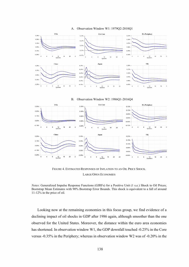
138
A. Observation Window W1: 1979Q2-2010Q1
B. Observation Window W2: 1986Q1-2016Q4
FIGURE 4. ESTIMATED RESPONSES OF INFLATION TO AN OIL PRICE SHOCK.
LARGE/OPEN ECONOMIES
Notes: Generalized Impulse Response Functions (GIRFs) for a Positive Unit (1 s.e.) Shock to Oil Prices;
Bootstrap Mean Estimates with 90% Bootstrap Error Bounds. This shock is equivalent to a fall of around
11-12% in the price of oil.
Looking now at the remaining economies in this focus group, we find evidence of a
declining impact of oil shocks in GDP after 1986 again, although smoother than the one
observed for the United States. Moreover, the distance within the euro area economies
has shortened. In observation window W1, the GDP downfall touched -0.25% in the Core
versus -0.35% in the Periphery; whereas in observation window W2 was of -0.20% in the

139
Core versus -0.25% in the Periphery. This result matches the increased synchronicity
across the euro area members after the euro adoption found by Aguiar-Conraria et al.
(2013) although using a different methodology (wavelet analysis) and data (Economic
Sentiment Indexes).
The empirical evidence exhibited in observation window W2, whereby the impact of
oil shocks turns negative, and statistically significant, around the 12th quarter, despite
being “demand-driven”, with exception only to China, likely corroborates the conjecture
made by Blanchard and Gali (2007), when arguing that “if the price of oil rises as a result
of, say, higher Chinese demand, this is just like an exogenous oil supply shock for the
remaining countries.” p. 17. By the same token, those results go against the conclusion
that oil demand shocks did not have a significant (adverse) impact on oil-importing
countries, as sustained by Baumeister and Hamilton (2019), after an empirical analysis
based on sign restrictions to identify the composition of oil shocks.
Finally, all GIRFs fade out around or even before the 24th quarter. This outcome
seems consistent with a temporary oil shock, as it is the case of the experiment undertaken
in the present work. Moreover, we should not expect an irreversible downward effect on
real GDP even from a permanent oil price shock, as shown by Aguiar‐Conraria and Wen
(2007).
We address now the impact of oil price shocks on inflation. Figure 4 displays the
related GIRFs for focus group I, that is the estimated responses of inflation to a positive
one standard error shock to the price of oil. Its size is always the same, equivalent to an
increase in the oil prices of around 11-12%.
On impact, the effect in the United States (22-21%) is considerably higher than for
the other economies in both the observation windows (Panels A and B). Namely, around
0.09-0.10% for the euro-area Core; 0.07-0.08% for the euro-area Periphery; 0.05-0.07%
for China; 0.08-0.09% for Japan and 0.09-0.12% for the United Kingdom. Similar results,
in particular, stronger effects on the United States inflation in comparison with the euro
area, have been found by Dees et al. (2007, p. 23) and by Cashin et al. (2014, see Figures
2 and 4). Differences in the transmission mechanism are the explanation advanced by
Peersman and Van Robays (2009). The direct pass-through effects of energy prices rise
are arguably stronger in the United States rather than in the European economies.

140
A. Observation Window W1: 1979Q2-2010Q1
B. Observation Window W2: 1986Q1-2016Q4
FIGURE 5. ESTIMATED RESPONSES OF SORT-TERM INTEREST RATES TO AN OIL PRICE SHOCK.
LARGE/OPEN ECONOMIES
Notes: Generalized Impulse Response Functions (GIRFs) for a Positive Unit (1 s.e.) Shock to Oil Prices;
Bootstrap Mean Estimates with 90% Bootstrap Error Bounds. This shock is equivalent to a fall of around
11-12% in the price of oil.
For the United States, the European economies, and the United Kingdom, the effects of
the oil price shock on inflation die out faster in the second observation window (Panel B),
thus showing conformity with the Great Moderation environment. But it is worth noting
that the euro-area Periphery lags the U.S., as well as the euro-area Core and the United

141
Kingdom changing patterns. And that persistent sluggish reaction happened despite the
convergence in the short-term interest rates across the euro area, as we will see next.
Figure 5 presents the responses of short-term interest rates to an oil price shock for
focus group I. Some salient features become apparent when confronting the dynamical
analysis (GIRFs) displayed in Panel A with Panel B, or loosely speaking when
heightening the Great Moderation support.
First, the responses of short-term interest rates were statistically significant only for
the euro-area economies in observation window W1. The primacy of the Bundesbank rule
might be an appropriate qualificative for the European forerunner in this domain. Second,
exception made to Japan, which has been confronted with the zero lower bound since the
late 1990s, the responses of short-term interest rate became significant in observation
window W2 for all countries/regions in focus group I. Third, the response of the United
States turned faster along with the Great Moderation. The peak is reached at the first
quarter in observation window W2 whereas it had been at the third quarter in observation
window W1.
Some further notes to interpret the results found for short-term interest rates responses
combined with those reported for inflation and the real GDP. After the Great Moderation,
we can see smoother negative impacts of oil shocks on GDP, prompt but milder short-
term interest rates reactions and faster inflation adjustments. Without disregarding the
already mentioned declining energy intensity and the possible change in the composition
of the oil price shocks, we may conclude with an insight of Blanchard and Gali (2007, p.
5): “The stronger commitment by central banks to maintaining a low and stable rate of
inflation …may have led to an improvement in the policy trade-off that make it possible
to have a smaller impact of a given oil price increase on both inflation and output
simultaneously”.
4.2 Euro Adopters
We tackle now the earlier euro adopters, excluding Luxembourg, but adding Denmark,
whose currency is pegged to the euro. Hence, as already noted in above, focus group II
comprehends Germany, France, Netherlands, Austria, Belgium, and Denmark, within the
euro-area Core; and Italy, Spain, Ireland, Greece, Portugal and Finland, within the euro-
area Periphery.

142
A. Observation Window W1: 1979Q2-2010Q1
B. Observation Window W2: 1986Q1-2016Q4
FIGURE 6. ESTIMATED RESPONSES OF REAL OUTPUT TO AN OIL PRICE SHOCK.
EURO ADOPTERS
Notes: Generalized Impulse Response Functions (GIRFs) for a Positive Unit (1 s.e.) Shock to Oil Prices;
Bootstrap Mean Estimates with 90% Bootstrap Error Bounds. This shock is equivalent to a fall of around
11-12% in the price of oil. Focus Group II (Euro adopters): The euro area members plus Denmark.
Figure 6 portrays the GIRFs of oil shocks on real GDP. Overall the effects are
statistically significant. However, with respect to the Core countries, this is the case only

143
in observation window W2, despite the milder responses. The GIRF of Germany seems
of particular interest in this context while being the developed economy that has most
benefited from the expansion of the large emerging and transition economies, namely
China, as illustrated by Figure 2. For observation window W2, the estimated effect of the
oil price shocks on the German real GDP is positive over the first year, reaching the peak
of 0.35% in the second quarter, but it turns negative between the sixth and the 18th
quarter, touching the trough of -0.27% at the 12th quarter.
We suggest that the initial comovements of the oil prices and the German GDP reflect
the demand effect, and where the oil price surge conveys the signal of an increase in
global demand. Although, in the medium run, the model captures the second-round
effects of an oil price shock on the German net energy-importing foreign counterparts, on
top of the adverse specific impact of higher energy prices in its domestic economy and
those stemming from the price stabilization monetary policy reaction.
We look now to the GIRFs at the troughs across the remaining Core and the Peripheral
countries when moving from observation window W1 to observation window W2. The
following comments seem pertinent.
First, and as already noted, the reactions of the output to oil shocks are milder in the
second sub-sample, overlapping the Great Moderation. And again, the change towards
moderation is more noticeable in the Peripheral countries, denoting convergence to the
Core. The median of the troughs lowered from -0.42% to -0.27% in the Periphery;
whereas only from -0.26% to -0.23% in the euro-area Core (see Table A. 1 in Appendix
A).
Second, the dispersion of the effects is higher in the euro-area Periphery. The standard
errors of the troughs are 0.20% in observation window W1 and 0.10% in observation
window W2 for the Periphery versus 0.06 % in both observation windows for the Core.
Portugal, Ireland and Finland are the countries where oil shocks have harsh impacts on
real GDP. Hence, the results denote accordance with the findings of Aguiar-Conraria and
Joana Soares (2011), where those same countries plus Greece showed the less
synchronized business cycle with the rest of Europe over the period 1975-2010.
Third, the responses of real GDP in Portugal and Greece offer both expected and
unexpected, even contradictory, profiles. Portugal industrial specialization was based on
traditional industries (e.g., textiles), as such, being more exposed to the increasing

144
A. Observation Window: 1979Q2-2010Q1
B. Observation Window: 1986Q1-2016Q4
FIGURE 7. ESTIMATED RESPONSES OF INFLATION TO AN OIL PRICE SHOCK.
EURO ADOPTERS
Notes: Generalized Impulse Response Functions (GIRFs) for a Positive Unit (1 s.e.) Shock to Oil Prices;
Bootstrap Mean Estimates with 90% Bootstrap Error Bounds. This shock is equivalent to a fall of around
11-12% in the price of oil. Euro adopters: The euro area members plus Denmark.

145
competition of the large emerging economies. Given that, an oil demand shock is typically
assimilated to an exogenous oil supply shock as pointed out by Blanchard and Gali
(2007). A flat response of the Portuguese GDP in the first year (contrasting with the rise
in Germany), followed by a decline from the second throughout the fourth year, fits its
economic structure well. Greece, another peripheral country with roughly the same real
GDP per capita as Portugal, shows an entirely different reaction. In observation window
W1 the response to the oil price shock is even positive; in observation window W2, it is
not statistically significant. The discrepant responses of the Portuguese and Greek outputs
to the oil shocks illustrate the higher degree of heterogeneity across the Peripheral
countries.
We turn now to the effects of oil price shocks on inflation across the euro adopters.
By inspecting the GIRFs portrayed in Figure 7, we get some information that the
aggregate for euro-area Core did not convey – namely, the earlier and predominant
German flavor. Earlier, in the sense that inflation adjustment was already fast in Germany
over the period tracked by observation window W1. Predominant, while exhibiting the
pattern to which the remaining countries in the euro-area Core, notably France, converged
(see Panel B in Figure 7).
Concerning the Peripheral countries, the responses of inflation denote a non-
convergent pattern to the Core, as already noted when reporting the results for its
aggregate (i.e., the GIRFs displayed in Figure 4 for the euro-area Periphery as a whole
region).
The case of Italy, as the larger economy in the euro-area Periphery, seems of
particular interest. As we can see in Figure A. 1 (in Appendix A), portraying the GIRFs
for the short-run interest rate response to an oil price shock, the estimated responses of
Italy are statistically significant and somewhat resembling Germany´s. More precisely, in
both observation windows, the peak is around 0.05% for Italy versus 0.04% for Germany,
and the average across the first year is 0.04% versus 0.03%. However, the stabilization
of inflation remained sluggish in Italy in observation window W2. We suggest that the
explanation might be found in the labor market rigidities prevalent in Italy19.
19 See, for example, Brunnermeier et al. (2016, Chapter 12, Loc. 4529) for a summary description of the
“restrictive” Italian labor market.

146
4.3 Robustness
Oil prices provide the opportunity to simultaneously test mounting inflation and
decreasing output. Therefore, they look a nice “conceptual experiment”20 to test
heterogeneities across the economic structure of a currency union member states. We do
not know an alternative disturbance with similar effects. But we can check the responses
of the real output to a common adversarial shock. A global negative shock to the real
prices of equity likely offers that possibility.
Recall that financial interlinkages framed within an international setting was precisely
at the heart of the seminal work of Pesaran et al. (2004) when building the GVAR
methodology. Therefore, we entertained a global shock on the real equity prices over
observation windows W1 and W2. The GIRFs for the 12 euro adopters (including
Denmark) are portrayed in Figure A. 2, in Appendix A. For a forthright comparison with
the results previously obtained from the oil shocks, Table A. 1 and Table A. 2 report the
estimated values at the troughs and their elementary statistics (i.e., the medians and the
standard errors).
The results from the shock on the real prices of equity are aligned with those obtained
from the oil shocks in the following items. First, Germany, showed the larger (lagged)
adverse effect across the Core economies in observation window W1; and converged to
the median of the Periphery in observation window W221. Second, Portugal showed the
larger adverse effect across the Peripheral economies in observation window W1; and
converged to the median of the Periphery in observation window W2. Third, the degree
of heterogeneity in the Periphery has dropped. However, the results are misaligned where
not showing now the convergence of the output responses of the euro-area Periphery as
region to the euro-area Core.
5. CONCLUSION
Output and inflation were the macroeconomic variables of interest to evaluate the
evolution of economic structures across the euro area member states as the euro
20 Here, we borrow the “conceptual experiment” expression from Pesaran and Shin (1998, p. 18). 21 Bayoumi and Eichengreen (2018) have found similar results for the period after the Maastrich Treaty.
Namely, the alignment of the output responses of Germany to “shocks to aggregate demand and
sometimes also to aggregate supply” with the Periphery.

147
experiment moved ahead. And oil shocks were the selected conceptual experiment to
undertake that study. The GVAR was the adopted methodology, although assuming oil
prices as a “dominant variable”. As expected, the responses (GIRFs) exhibit temporary
effects; that is, the disturbed variables have adjusted to their initial levels. But somehow
in contradiction with the more recent oil literature, they were statistically significant (or
very close to) even when oil demand shocks were prevalent. More specific results are
highlighted next.
The empirical evidence obtained for Germany is noticeable for three reasons. First, it
is illustrative of the merits of the methodology employed. Measured by exports weighted
by GDP, Germany was the European economy that has most beneficiated from the
expansion of the Chinese economy. Oil demand shocks were prevalent in that same
period, tracked by our second observation window W2, spanning from 1986Q1 through
2016Q4. The estimated effects of oil shocks on the Germany output revealed positive on
impact, a la Kilian (2009), and turned into negative around the 12th quarter, a la
Blanchard (2006). Second, the Germany stance on fast stabilization of inflation has
defined the adjustment pattern later exhibited by all developed economies, including the
United States. Third, the convergence of the larger (lagged) negative responses of the
German output to global shocks towards the median of the euro-area Periphery.
Concerning the Periphery, the results point to decreasing heterogeneity across that
region (notably for Portugal), and convergence towards the Core. However, the latter was
not verified when using an alternative experiment to oil shocks, namely a negative global
shock to the real prices of equity.
Finally, inflation estimated responses to oil shocks were clearly distinct between the
Core and the Periphery. Furthermore, there was no evidence of improvement on the
sluggish adjustment of inflation in the Periphery to a global shock as the euro experiment
went ahead.

148
APPENDIX A
A. Observation Window 1979Q2-2010Q1
B. Observation Window 1986Q1-2016Q4
FIGURE A. 1. ESTIMATED RESPONSES OF SORT-TERM INTEREST RATES TO AN OIL PRICE SHOCK.
EURO ADOPTERS
Notes: Generalized Impulse Response Functions (GIRFs) for a Positive Unit (1 s.e.) Shock to Oil Prices;
Bootstrap Mean Estimates with 90% Bootstrap Error Bounds. This shock is equivalent to a fall of around
11-12% in the price of oil. Denmark is not included because of data limitations.
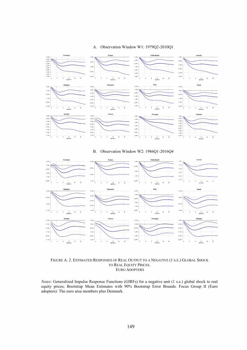
149
A. Observation Window W1: 1979Q2-2010Q1
B. Observation Window W2: 1986Q1-2016Q4
FIGURE A. 2. ESTIMATED RESPONSES OF REAL OUTPUT TO A NEGATIVE (1 S.E.) GLOBAL SHOCK
TO REAL EQUITY PRICES.
EURO ADOPTERS
Notes: Generalized Impulse Response Functions (GIRFs) for a negative unit (1 s.e.) global shock to real
equity prices; Bootstrap Mean Estimates with 90% Bootstrap Error Bounds. Focus Group II (Euro
adopters): The euro area members plus Denmark.

150
TABLE A. 1–Troughs of the GIRFs for the Real GDP after a Positive (1 s.e.) Shock to Oil Prices
Country Trough
Observation Window W1 Observation Window W2
1979Q2-2010Q1 1986Q1-2016Q4
EA-Core
Germany -0.41% -0.27%
France -0.24% -0.17%
Netherlands -0.27% -0.29%
Austria -0.25% -0.32%
Belgium -0.26% -0.17%
Denmark -0.27% -0.19%
Median -0.26% -0.23%
SE 0.06% 0.06%
EA-Periphery
Italy -0.31% -0.24%
Spain -0.25% -0.13%
Ireland -0.54% -0.44%
Greece -0.22% -0.24%
Portugal -0.78% -0.31%
Finland -0.52% -0.35%
Median -0.42% -0.27%
SE 0.20% 0.10%
Notes: The generalized impulse response functions (GIRFs) are shown in Figure 6. The troughs have been
extracted from the Output files, “\gvarOIL_79_2010\GIRFs\DOMINANT UNIT MODEL 1se pos shock
to OIL PRICES” (see the Excel sheet <graphs_bs REAL GDP per capita_edited>) and from
“\gvarOIL_86_2016\GIRFs\DOMINANT UNIT MODEL 1se pos shock to OIL PRICES”, available at the
supplemental link.

151
TABLE A. 2–Troughs of the GIRFs for the Real GDP after a Negative (1 s.e.) Global Shock
to Real Equity Prices
Country Trough
Observation Window W1 Observation Window W2
1979Q2-2010Q1 1986Q1-2016Q4
EA-Core
Germany -1.61% -0.96%
France -0.86% -0.63%
Netherlands -1.21% -0.98%
Austria -1.08% -1.20%
Belgium -1.11% -0.70%
Denmark -0.90% -0.62%
Median -1.09% -0.83%
SE 0.25% 0.21%
EA- Periphery
Italy -1.01% -0.91%
Spain -0.83% -0.46%
Ireland -1.40% -1.30%
Greece -0.81% -0.95%
Portugal -2.62% -0.92%
Finland -1.63% -1.26%
Median -1.01% -0.93%
SE 0.63% 0.27%
Notes: The graphs of the generalized impulse response functions (GIRFs) are available at the Output file
in the supplemental link. The troughs have been extracted from the files
“\gvarOIL_79_2010\GIRFs\DOMINANT UNIT MODEL 1se pos shock to OIL PRICES” (see the Excel
sheet <graphs_bs REAL GDP per capita_edited>) and from “\gvarOIL_86_2016\GIRFs\DOMINANT
UNIT MODEL 1se pos shock to OIL PRICES” (see the Excel sheet <graphs_bs REAL GDP per
capita_edited>), available at that same Output file in the supplemental link.

152
APPENDIX B
MODELING SHOCKS TO OIL PRICES IN A DOMINANT UNIT
The purpose of this Appendix is to show that shocks to oil prices when oil prices is
modeled in a “dominant unit” preserve the meaning of a structural innovation without
waiving the effects of cross-correlated shocks captured by the generalized impulse
response functions (GIRFS) in a GVAR framework.
For the sake of clarity, we start by writing, straightforward, the VARX*(𝑝, 𝑞) model
for the individual country i, but before the inclusion of a common variable22:
𝑥𝑖𝑡 = 𝑎𝑖0 + 𝑎𝑖1𝑡 + 𝛷𝑖1𝑥𝑖,𝑡−1 + … + 𝛷𝑖𝑝𝑥𝑖,𝑡−𝑝𝑖 + 𝛬𝑖0𝑥𝑖𝑡
∗
+ 𝛬𝑖1𝑥𝑖,𝑡−1∗ + . . . + 𝛬𝑖𝑞𝑖𝑥𝑖,𝑡−𝑞𝑖
∗ + 𝑢𝑖𝑡
(1)
where 𝒙𝑖𝑡 is a 𝑘𝑖 × 1 vector of domestic variables, 𝒙𝑖𝑡∗ is a 𝑘𝑖
∗ × 1 vector of foreign (star)
variables, and 𝒖𝑖𝑡 is a vector of idiosyncratic country-specific shocks, for 𝑡 =
1, 2, . . . , 𝑇.
The vector of foreign variables is defined as
𝑥𝑖𝑡∗ =∑𝑤𝑖𝑗𝑥𝑗𝑡 , 𝑤𝑖𝑖 = 0
𝑁
𝑗=0
(2)
with 𝑤𝑖𝑗, 𝑗 = 0, 1, 2, . . . , 𝑁, a set of weights such that ∑ 𝑤𝑖𝑗𝑁𝑗=0 = 1. The weights are
commonly based on the trade (imports plus exports) share of country j in country i.
In matrix notation (2) is written as
𝑥𝑖𝑡∗ = �̃�𝑖
′𝑥 (3)
22 See Chudik and Pesaran (2016) for a compact description of the GVAR methodology and Smith and
Galesi (2014, User Guide) for a more detailed presentation, in particular the procedures to include a
dominant unit in the GVAR, pp. 152-8.

153
where �̃�𝑖 ≡ [𝑤𝑗𝑖] is the 𝑘 × 𝑘𝑖∗ matrix of country-specific weights and 𝒙𝑡 =
(𝒙0𝑡′ , 𝒙1𝑡
′ , . . . , 𝒙𝑁𝑡′ )′ is 𝑘 × 1 vector collecting all endogenous variables in the global
model (including the U.S., indexed by 0); as such 𝑘 = ∑ 𝑘𝑖𝑁𝑖=0 .
We rewrite now the VARX*(p, q) model for country i, but augmented of one
common variable 𝑤𝑡 23
𝑥𝑖𝑡 = 𝑎𝑖0 + 𝑎𝑖1𝑡 + 𝛷𝑖1𝑥𝑖,𝑡−1 + … + 𝛷𝑖𝑝𝑥𝑖,𝑡−𝑝𝑖 + 𝛬𝑖0𝑥𝑖𝑡∗ + 𝛬𝑖1𝑥𝑖,𝑡−1
∗
+ . . . + 𝛬𝑖𝑞𝑖𝑥𝑖,𝑡−𝑞𝑖∗ + 𝜓𝑖0𝑤𝑡 + 𝜓𝑖1𝑤𝑡−1+ . . . + 𝜓𝑖𝑞𝑖𝑊
𝑤𝑡−𝑞𝑖𝑊+ 𝑢𝑖𝑡
(4)
where 𝑤𝑡 is determined in a univariate “dominant unit” model (i.e., the marginal model24),
which is defined as follows, when including lagged “feedback variables”:
𝑤𝑡 = 𝜇0 + 𝜇1𝑡 + 𝜙𝑤1𝑤𝑡−1+ . . . +𝜙𝑤�̃�𝑤𝑡−�̃� + 𝜆1′ �̃�𝑡−1+ . . . +𝜆�̃�
′ �̃�𝑡−�̃�
+ 𝜂𝑡 (5)
and where 𝒙𝑡 is a 𝑘𝑤∗ × 1 vector of global cross-sections averages and 𝝀𝑗 , 𝑗 = 1, . . . , �̃�, is
the 𝑘𝑤∗ × 1 dimensional vector collecting the 𝜆𝑗𝑙𝑤 coefficients associated with the
𝑙𝑤𝑡ℎglobal variable, �̃�𝑙𝑤,𝑡−𝑗. In matrix notation the “feedback variables” are written as
�̃�𝑡 = �̃�𝑤𝑥𝑡 (6)
where �̃�𝑤 is 𝑘𝑤∗ × 𝑘 weight matrix, assumed time invariant, and 𝒙𝑡 =
(𝒙0𝑡′ , 𝒙1𝑡
′ , . . . , 𝒙𝑁𝑡′ )′ is the vector of global endogenous variables.
It is worth noting that only the “lagged” although not the contemporaneous values of
�̃�𝑡 enter equation (5), as �̃�𝑡 is not weakly exogenous for the parameters of the dominant
unit model25.
23 We keep 𝑤𝑡 to represent the dominant variable as the common practice in the GVAR literature. The
context and the different sort of indexation make clear the distinction to the trade weights notation ( 𝑤𝑖𝑗). 24 For a definition of “conditional” and of “marginal” models see, for ex., Garratt et al. (2006, pp. 58-59). 25 See Lütkepohl and Krätzig (2004, pp. 99 and 108) for the definition of a weakly exogeneity in its
general terms and in the context of cointegration. See Garratt et al. (2006, pp. 57-59) for a formal
treatment and for the definition of a “long-run” forcing a weakly exogenous I (1) variable.

154
The country-specific conditional models (4) and the marginal model (5) must be
combined and solved for the “complete” global VAR model. To start the procedure, we
have to get rid of the star variables. Hence, define 𝒛𝑖𝑡 = (𝒙𝑖𝑡′ , 𝒙𝑖𝑡
∗′)′, a vector of dimension
(𝑘𝑖 + 𝑘𝑖∗) × 1; and after making 𝑝𝑖 = 𝑞𝑖, rewrite equation (4) as follows:
𝐴𝑖0𝑧𝑖𝑡 = 𝑎𝑖0 + 𝑎𝑖1𝑡 + 𝐴𝑖1𝑧𝑖,𝑡−1 +⋯+ 𝐴𝑖𝑝𝑖𝑧𝑖,𝑡−𝑝𝑖
+ 𝜓𝑖0𝑤𝑡 + 𝜓𝑖1𝑤𝑡−1+ . . . + 𝜓𝑖𝑞𝑖𝑊𝑤𝑡−𝑞𝑖𝑊
+ 𝑢𝑖𝑡
(7)
with
𝐀𝑖0 = (𝐈𝑘𝑖 , −𝚲𝑖0), 𝐀𝑖𝑗 = (𝚽𝑖𝑗, 𝚲𝑖𝑗), for 𝑗 = 1, . . . , 𝑝𝑖
and where 𝑨𝑖0 and 𝑨𝑖𝑗 are 𝑘𝑖 × (𝑘𝑖 + 𝑘𝑖∗) dimensional matrices; and 𝑨𝑖0 is non-singular.
Define, now, the (𝑘𝑖 + 𝑘𝑖∗) × 𝑘 link matrices
W𝑖 = (E𝑖′, W̃𝑖
′), (8)
where 𝑬𝑖 is the 𝑘 × 𝑘𝑖 dimensional selection matrix that select 𝒙𝑖𝑡, namely 𝒙𝑖𝑡 = 𝑬𝑖′𝒙𝑡
and �̃�𝑖 is the weight matrix introduced in (3).
Therefore, we may substitute 𝒛𝑖𝑡 in (7) for 𝑾𝑖𝒙𝑡 and get rid of the exogenous (star)
variables, 𝒙𝑖𝑡∗ , while preserving the VARX* coefficients already estimated.
𝛢𝑖0𝑊𝑖𝑥𝑡 = 𝑎𝑖0 + 𝑎𝑖1𝑡 + 𝛢𝑖1𝑊𝑖𝑥𝑡−1 +⋯+ 𝛢𝑖𝑝𝑖𝑊𝑖𝑥𝑡−𝑝𝑖 +⋯
+ 𝜓𝑖0𝑤𝑡 +𝜓𝑖1𝑤𝑡−1+ . . . + 𝜓𝑖𝑞𝑖𝑊𝑤𝑡−𝑞𝑖𝑊
+ 𝑢𝑖𝑡 (9)
to build the global system we just need to stack all those equations, i.e., the expression
given in (9) for the 𝑖 = 0, 1, 2, . . . , 𝑁 countries,
𝐺0𝑥𝑡 = 𝑎0 + 𝑎1𝑡 + 𝐺1𝑥𝑡−1 +⋯+ 𝐺𝑝𝑥𝑡−𝑝 +⋯
+ 𝜓0𝑤𝑡 + 𝜓1𝑤𝑡−1+ . . . + 𝜓𝑝𝑤𝑡−p + 𝑢𝑡
(10)

155
where 𝑮0 and 𝑮𝑗, with 𝑗𝑡 = 1, . . . , 𝑝, are 𝑘 × 𝑘 matrices, and 𝒂0, 𝒂1and 𝒖𝑡are
𝑘 × 1vectors:
𝐺0=
NN WA
WA
WA
0
110
000
, 𝐺𝑗 =
NNj
j
j
WA
WA
WA
11
00
,
𝑎0=(
𝑎00𝑎10⋮𝑎𝑁0
), 𝑎1 = (
𝑎01𝑎11⋮𝑎𝑁1
), 𝜓𝑗=
(
𝜓0𝑗𝜓1𝑗⋮𝜓𝑁𝑗)
, 𝑢𝑡=(
𝑢0𝑡𝑢1𝑡⋮𝑢𝑁𝑡
) (11)
and 𝑝 = 𝑚𝑎𝑥{𝑚𝑎𝑥 𝑝𝑖 , 𝑚𝑎𝑥 𝑞𝑖 , 𝑚𝑎𝑥 𝑞𝑖𝑊 }.
Next, we solve the system for the global 𝑘 × 1 vector of endogenous variables 𝒙𝒕 =
(𝒙𝟎𝒕′ , 𝒙𝟏𝒕
′ , ⋯ , 𝒙𝑵𝒕′ )′ “combined” with the dominant variable 𝑤𝑡, which is preserved as
weakly exogenous. Define the (𝑘 + 1) × 1 vector of all observable variables 𝒚𝑡 =
(𝒙𝑡′ , 𝑤𝑡)
′ and, after making 𝑝 = 𝑝 = �̃�, stack equations (5) and (10) to obtain the
“combined model”:
𝐻0𝑦𝑡 = ℎ0 + ℎ1𝑡 + 𝐻1𝑦𝑡−1 +⋯+𝐻𝑝𝑦𝑡−𝑝 + 𝜁𝑡 (12)
where
𝑯0 = (𝑮0 −𝝍0𝟎1×𝑘 1
), 𝒉0 = (𝒂0𝜇0), 𝒉1 = (
𝒂1𝜇1)
𝑯𝑗 = (𝑮𝑗 𝝍𝑗
𝝀𝑗′�̃�𝑤 𝜙𝑤𝑗
) , 𝑗 = 1, . . . , 𝑝, 𝜻𝑡 = (𝒖𝑡𝜂𝑡)
Assuming that 𝑮0−1exists the matrix 𝑯0 is invertible:
𝐻0−1 = (𝐺0
−1 −𝐺0−1𝜓0
0 1)
(13)
156
which is block higher triangular, “showing the casual nature of the common (dominant)
variables, 𝑤𝑡”, as highlighted by Chudik and Pesaran (2016:170).
Finally, multiplying both sides of (12) by 𝑯0−1we obtain the “complete” GVAR
model:
𝑦𝑡 = 𝑐0 + 𝑐1𝑡 + 𝐶1𝑦𝑡−1 +⋯+ 𝐶𝑝𝑦𝑡−𝑝 + 𝐻0−1𝜁𝑡 (14)
with
𝒄𝑗 = 𝑯0−1𝒉𝑗 , 𝑗 = 0, 1; 𝑪𝑗 = 𝑯0
−1𝑯𝑗, 𝑗 = 1, . . . , 𝑝
For which the moving average representation is given by
𝑦𝑡 = 𝑑𝑡 +∑𝐵𝑠𝜀𝑡−𝑠
∞
𝑠=0
= 𝜀𝑡 + 𝐵1𝜀𝑡−1 + 𝐵2𝜀𝑡−2+. .. (15)
where 𝒅𝑡 represents the deterministic component of 𝒚𝑡, 𝑩𝑠 can be derived recursively as
𝐵𝑠 = 𝐶1𝐵𝑠−1 + 𝐶2𝐵𝑠−2+. . . +𝐶𝑝𝐵𝑠−𝑝, 𝑠 = 1, 2, . ..
with 𝐵0 = 𝐼𝑘+1, 𝐵𝑠 = 0, for 𝑠 < 0 (16)
and 𝜺𝑡 = (𝜺0𝑡′ , 𝜺1𝑡
′ , 𝜺2𝑡′ , . . . , 𝜺𝑁𝑡
′ , 𝜀𝑤𝑡)′ is given by
𝜀𝑡 = 𝐻0
−1𝜁𝑡 = (𝐺0−1(𝑢𝑡 − 𝜂𝑡𝜓0)
𝜂𝑡) (17)
Looking at (17) we can see that 𝜀𝑤𝑡 = 𝜂𝑡. Recall now that 𝜂𝑡 is the disturbance term in
the dominant variable 𝑤𝑡 model, that is, the “marginal model” expressed in (5). Hence,
shocks to 𝑤𝑡 equation in the MA (∞) representation (15) are preserved as structural
innovations.

157
Let us now write the GIRFs for the GVAR model expressed in (15), for a shock
defined by 𝑣𝑡 = 𝑒𝑙′𝜻𝑡 at time t, where 𝒆𝑙 = (0, 0, . . . , 0, 1, 0, . . . 0)
′ is the selection
vector, with unity at the 𝑙𝑡ℎ element:
𝐺𝐼𝑅𝐹(ℎ, 𝑦𝑡; 𝑧𝑡) = 𝐸 (𝑦𝑡+ℎ|𝑣𝑡 = √𝑒𝑙
′𝛺𝜁𝑒𝑙 , 𝛵𝑡−1) − 𝐸𝑦(𝑡 + ℎ|𝛵𝑡−1)
=𝐵ℎ𝐻0
−1𝛺𝜁𝑒𝑙
√𝑒𝑙′𝛺𝜁𝑒𝑙
, ℎ = 0, 1, 2, . . . ,
(18)
Where 𝛵𝑡−1 is the information set up to time 𝑡 − 1, 𝑩ℎ is computed as in (16), and 𝜴𝜁is
the covariance matrix of the “combined model” error terms, that is of the model expressed
in (12).
To show that the structural impulse responses (SGIRF) for a common variable
modeled in a dominant unit simplifies to the GIRF written in (18), we reproduce next the
SGIRF definition given in Smith and Galesi (2014:157-58), after small adjustments to
harmonize the notation:
𝑆𝐺𝐼𝑅𝐹(ℎ, 𝑦𝑡; 𝑣𝑡) = 𝐸 (𝑦𝑡+ℎ|𝑣𝑡 = √𝑒𝑙′𝛴𝑣𝑒𝑙, 𝛵𝑡−1) − 𝐸(𝑦𝑡+ℎ|𝛵𝑡−1)
=𝐵ℎ(𝑃𝐻𝑜𝐻0)
−1𝛴𝑣𝑒𝑙
√𝑒𝑙′𝛴𝑣𝑒𝑙
, ℎ = 0, 1, 2, . . .,
(19)
where the matrix 𝑷𝐻𝑜 come from the standard Cholesky decomposition to identify the
structural innovations in a “block” formed by the dominant unit and the U.S. economy
(Smith and Galesi 2014: 157), and the index v refers to the vector of error terms 𝒗𝑡 =
(𝒖1𝑡′ , . . . , 𝒖𝑁𝑡
′ , �̇�𝑡′ ), where �̇� stands for the vector of structural shocks in the system of
equations written for the “block”.
While having only one, already identified, structural innovation 𝜀𝑤𝑡 = 𝜂𝑡, as shown
in (17), we may drop 𝑷𝐻𝑜. Moreover, for a “block” formed by one single dominant
variable, 𝑤𝑡, 𝒗𝑡 = (𝒖1𝑡′ , . . . , 𝒖𝑁𝑡
′ , �̇�𝑡′ ) = (𝒖1𝑡
′ , . . . , 𝒖𝑁𝑡′ , 𝜂𝑡)
′, implying that 𝐶𝑜𝑣(𝒗𝑡) =
𝐶𝑜𝑣(𝜻) or 𝜮𝑣 = 𝜴𝜁. Therefore, both the numerator and denominator of (19) collapse into
their counterparts in (18).

158
It should be noticed that when 𝑙 = 𝑘 + 1, where 𝑘 + 1 indexes the common
(dominant) variable, the denominator in (19) renders the standard deviation of the
structural innovation in the “marginal model”, viz. √𝑒𝑙′𝜮𝑣𝑒𝑙 = √𝑒𝑙
′𝜴𝜁𝑒𝑙 = √𝐸(𝜀𝑤𝑡2 ) =
𝜎𝜂.
Finally, it might be interesting to explain the meaning of “structural” within the
framework of a generalized impulse response function by inspecting the covariance
matrix of the error terms. Hence, let us write the (𝑘 + 1) × (𝑘 + 1) dimensional
covariance matrix of the country specific residuals 𝒖𝑡 and the structural shock 𝜂𝑡
𝐶𝑜𝑣(𝒗𝑡) = (
𝑉𝑎𝑟(𝒖1𝑡) ⋯ 𝐶𝑜𝑣(𝒖1𝑡, 𝒖𝑁𝑡) 𝐶𝑜𝑣(𝒖1𝑡, 𝜂𝑡)⋮ ⋯ ⋮ ⋮
𝐶𝑜𝑣(𝒖𝑁𝑡, 𝒖1𝑡, ) ⋯ 𝑉(𝒖𝑁𝑡) 𝐶𝑜𝑣(𝒖𝑁𝑡, 𝜂𝑡)
𝐶𝑜𝑣(𝜂𝑡, 𝒖1𝑡, ) ⋯ 𝐶𝑜𝑣(𝜂𝑡 , 𝒖𝑁𝑡, ) 𝑉𝑎𝑟(𝜂𝑡)
)
= (𝜮𝑢 𝐶𝑜𝑣(𝒖, 𝜂𝑡)
𝐶𝑜𝑣(𝜂𝑡, 𝒖) 𝑉𝑎𝑟(𝜂𝑡))
When 𝑙 = 𝑘 + 1, the structural generalized impulse response functions for shock set to
one standard deviation (s.d.) of 𝜂 is written as
𝑆𝐺𝐼𝑅𝐹(ℎ, 𝑦𝑡; 𝑣𝑘+1,𝑡) =
(𝐵ℎ1 𝐵ℎ2𝑏ℎ1′ 𝑏ℎ2
) (𝐺0−1 −𝐺0
−1𝜓001×𝑘 1
) (𝐶𝑜𝑣(𝑢, 𝜂𝑡)
𝑉𝑎𝑟(𝜂𝑡))
𝜎𝜂
= (𝐵ℎ1 𝐵ℎ2𝑏ℎ1′ 𝑏ℎ2
) (𝜎𝜂−1𝐺0
−1(𝐼𝑘 − 𝜓0)𝐶𝑜𝑣(𝑢, 𝜂𝑡)𝜎𝜂
) ,
ℎ = 0, 1, 2, . . . ,
(20)
Equation (20) make the properties of the SGIRF immediately apparent: It is
“structural” in the sense of being entertained by an identified shock, 𝜎𝜂, and “generalized”
once reflecting the distribution of the errors across the different equations in the global

159
model, by taking into account their cross-correlations, in case captured by the term
𝐶𝑜𝑣(𝒖, 𝜂𝑡).
160
REFERENCES
Aguiar-Conraria, Luıs, and Maria Joana Soares (2011), "Business Cycle Synchronization
and the Euro: A Wavelet Analysis", Journal of Macroeconomics, 33(3), pp. 477-
89.
Aguiar-Conraria, Luís, Manuel M. F. Martins, and Maria Joana Soares (2013),
"Convergence of the Economic Sentiment Cycles in the Eurozone: A Time-
Frequency Analysis", Journal of Common Market Studies, 51(3), pp. 377-98.
Aguiar‐Conraria, Luís, and Yi Wen (2007), "Understanding the large negative impact of
oil shocks", Journal of Money, Credit and Banking, 39(4), pp. 925-44.
Ahlborn, Markus, and Marcus Wortmann (2018), "The core‒periphery pattern of
European business cycles: A fuzzy clustering approach", Journal of
Macroeconomics, 55, pp. 12-27.
Baumeister, Christiane, and James D. Hamilton (2019), "Structural Interpretation of
Vector Autoregressions with Incomplete Identification: Revisiting the Role of Oil
Supply and Demand Shocks", American Economic Review, 109(5), pp. 1873-910.
Baumeister, Christiane, and Gert Peersman (2013), "Time-Varying Effects of Oil Supply
Shocks on the US Economy", American Economic Journal: Macroeconomics,
5(4), pp. 1-28.
Bayoumi, by Tamim, and Barry Eichengreen (2018), "Aftershocks of Monetary
Unification: Hysteresis with a Financial Twist", Journal of Banking and Finance,
Available online 19 June 2018, Article 105365, pp. -.
Blanchard, Olivier (2006), "European unemployment: the evolution of facts and ideas",
Economic Policy, 21(45), pp. 5-59.
Blanchard, Olivier J., and Jordi Gali (2007), "The Macroeconomic Effects of Oil Shocks:
Why are the 2000s so Different from the 1970s?", National Bureau of Economic
Research Working Paper 13368.
Brunnermeier, Markus K, Harold James, and Jean-Pierre Landau (2016), The Euro and
the Battle of Ideas, Princeton, NJ: Princeton University Press.
Campos, Nauro F., Jarko Fidrmuc, and Iikka Korhonen (2019), "Business cycle
synchronisation and currency unions: A review of the econometric evidence using
meta-analysis", International Review of Financial Analysis, 61, pp. 274-83.
Carneiro, José Sá (2019), Portugal in the Euro - A GVAR Approach, Unpublished
manuscript, School of Economics and Management (FEP), University of Porto.
Cashin, Paul, Kamiar Mohaddes, Maziar Raissi, and Mehdi Raissi (2014), "The
differential effects of oil demand and supply shocks on the global economy",
Energy Economics, 44, pp. 113-34.
Chudik, Alexander, and M Hashem Pesaran (2013), "Econometric analysis of high
dimensional VARs featuring a dominant unit", Econometric Reviews, 32(5-6), pp.
592-649.
— (2016), "Theory and practice of gvar modelling", Journal of Economic Surveys, 1(30),
pp. 165-97.
Clarida, Richard, Jordi Galí, and Mark Gertler (1999), "The Science of Monetary Policy:
A New Keynesian Perspective", Journal of Economic Literature, 37(4), pp. 1661-
707.

161
De Haan, Jakob, Robert Inklaar, and Richard Jong‐A‐Pin (2008), "Will business cycles
in the euro area converge? A critical survey of empirical research", Journal of
Economic Surveys, 22(2), pp. 234-73.
Dees, Stéphane (2016), "Credit, asset prices and business cycles at the global level",
Economic Modelling, 54, pp. 139-52.
Dees, Stephane, Filippo di Mauro, M Hashem Pesaran, and L Vanessa Smith (2007),
"Exploring the international linkages of the euro area: a global VAR analysis",
Journal of Applied Econometrics, 22(1), pp. 1-38.
Fagan, Gabriel, and Vitor Gaspar (2007), "Adjusting to the Euro", European Central Bank
(ECB) Working Paper 716.
Frankel, Jeffrey A (1979), "On the mark: A theory of floating exchange rates based on
real interest differentials", American Economic Review, 69(4), pp. 610-22.
Garratt, Anthony, Kevin Lee, M. Hashem Pesaran, and Yongcheol Shin (2006), Global
and national macroeconometric modelling: a long-run structural approach, 2012
ed. Oxford, UK: Oxford University Press.
Hamilton, J. D. (2009), "Causes and consequences of the oil shock of 2007-08",
Brookings Papers on Economic Activity
Kilian, Lutz (2009), "Not all oil price shocks are alike: Disentangling demand and supply
shocks in the crude oil market", American Economic Review, 99(3), pp. 1053-69.
Koop, Gary, M Hashem Pesaran, and Simon M Potter (1996), "Impulse response analysis
in nonlinear multivariate models", Journal of Econometrics, 74(1), pp. 119-47.
Krugman, Paul (2001), "Lessons of Massachusetts for EMU'", International Library of
Critical Writings in Economics, 134, pp. 41-61.
Lütkepohl, Helmut, and Markus Krätzig (2004), Applied time series econometrics,
Cambridge, UK: Cambridge University Press.
McConnell, Margaret M, and Gabriel Perez-Quiros (2000), "Output fluctuations in the
United States: What has changed since the early 1980's?", American Economic
Review, 90(5), pp. 1464-76.
Mohaddes, Kamiar, and M Hashem Pesaran (2016), "Country-specific oil supply shocks
and the global economy: A counterfactual analysis", Energy Economics, 59, pp.
382-99.
Peersman, Gert, and Ine Van Robays (2009), "Oil and the Euro area economy", Economic
Policy, 24(60), pp. 603-03-51.
Pesaran, H Hashem, and Yongcheol Shin (1998), "Generalized impulse response analysis
in linear multivariate models", Economics Letters, 58(1), pp. 17-29.
Pesaran, M. Hashem, Til Schuermann, and Scott M. Weiner (2004), "Modeling regional
interdependencies using a global error-correcting macroeconometric model",
Journal of Business & Economic Statistics, 22(2), pp. 129-62.
Smith, L. Vanessa, and Alessandro Galesi. 2014. "GVAR Toolbox 2.0."
<https://sites.google.com/site/gvarmodelling/gvar-toolbox>.