Portfolio Selection in the Presence ofMultiple Criteria

Ralph E. Steuer∗

Terry College of BusinessUniversity of Georgia

Athens, Georgia 30602-6253 USA

Yue QiHedge Fund Research Institute

International University of MonacoPrincipality of Monaco

Markus HirschbergerDepartment of Mathematics

University of Eichstatt-IngolstadtEichstatt, Germany

Published in: Handbook of Financial Engineering, SpringerScience, New York, (2008), pp. 3-24

1 Introduction

There has been a growing interest in how to incorporate additional criteriabeyond “risk and return” into the portfolio selection process. In response,our purpose is to describe the latest in results that have been coming together

∗Corresponding author rsteuer@uga.edu

1

under the topic of multiple criteria portfolio selection. Starting with a reviewof conventional portfolio selection from a somewhat different perspective soas better to lead into the topic of multiple criteria portfolio selection, westart from basics as follows.

In portfolio selection, two vectors are associated with each portfolio. Oneis used to “define” a portfolio. The other is used to “describe” the portfolio.The vector used to define a portfolio is an investment proportion vector. Itspecifies the proportions of an amount of money to be invested in differentsecurities thereby defining the composition of a portfolio. The length of aninvestment proportion vector is the number of securities under consideration.

The other of a portfolio’s two vectors is a criterion vector. A portfolio’scriterion vector contains the values of measures used to evaluate the portfolio.For instance, in mean-variance portfolio selection, criterion vectors have twocomponents. One is for specifying the expected value of the portfolio’s returnrandom variable. The other is for specifying the variance of the randomvariable. The idea is that the variance of the random variable is a measureof risk. In reality, investors may have additional concerns.

To accommodate multiple criteria in portfolio selection, we no longer callan “efficient frontier” by that name. Instead we call it a “nondominatedfrontier” or “nondominated set.” Terminologically, criterion vectors are noweither nondominated or dominated. This does not mean that the term ef-ficiency has been discarded. Efficiency is simply re-directed to apply onlyto investment proportion vectors in the following sense. An investment pro-portion vector is efficient if and only if its criterion vector is nondominated,and an investment proportion vector is inefficient if and only if its criterionvector is dominated.

A portfolio selection problem is amultiple criteria portfolio selection prob-lem when its criterion vectors have three or more components. In conven-tional portfolio selection, with criterion vectors of length two, the nondom-inated set is typically a curved line in two-dimensional space, which whengraphed usually has expected value of the portfolio return random variableon the vertical axis and variance (or more commonly, standard deviation) ofthe same random variable on the horizontal axis. But, when criterion vec-tors are of length three or more, the nondominated set is best thought of asa surface in higher dimensional space. Because of the increased difficultiesinvolved in computing nondominated surfaces and communicating them toinvestors, multiple criteria portfolio selection problems can be expected tobe much more difficult to solve than the types of problems we are used to

2

seeing in conventional portfolio selection.Multiple criteria portfolio selection problems normally stem from multiple-

argument investor utility functions, but can stem from a single-argumentutility function.1 While portfolio selection problems with criterion vectors oflength two are the usual case with single-argument utility functions (whenthe argument is stochastic), it is possible for a multiple criteria portfolio se-lection problem to result from a single-argument utility function when theinvestor’s nondominated set is a consequence of three or more measures de-rived from the same single stochastic argument. An example of this is when amean-variance portfolio selection problem (which revolves around the singlerandom variable of portfolio return) is extended to take into account addi-tional measures, such as skewness, based upon the same random variable.

Despite the above, we will primarily focus on the more general and inter-esting cases of multiple criteria portfolio selection problems resulting frommultiple-argument utility functions. Beyond the random variable of portfo-lio return, utility functions can take additional stochastic and deterministicarguments. Additional stochastic arguments might include dividend, liquid-ity, and excess return over of a benchmark random variables. Deterministicarguments might include the number of securities in a portfolio, turnover,and amount of short selling.

Conventional mean-variance portfolio analysis (described as “modern port-folio analysis” in Elton, Gruber, Brown and Goetzmann (2002)) dates backto the papers of Roy (1952) and Markowitz (1952). In addition to intro-ducing new ways to think about finance, the papers are important becausethey symbolize different strategies for solving portfolio selection problems.In computing his “safety first” point, Roy’s paper symbolizes approachesthat attempt to compute directly portfolios whose criterion vectors possesspre-chosen characteristics.

On the other hand, the approach of Markowitz is more reflective. It rec-ognizes that there are likely to be differences among investors. It essentiallyeschews pre-conceived notions preferring to compute the entire nondominatedset first. Then, only after studying the nondominated set should an investorattempt to identify a most preferred criterion vector. Overall, Markowitz’ssolution approach consists of the following four stages.

1. Compute the nondominated set.

1Although we use the term utility function throughout, preference function or valuefunction could just have well been used.

3

2. Communicate the nondominated set to the investor.3. Select the most preferred of the points in the nondominated set.4. Working backwards, identify an investment proportion vector whose

image is the nondominated point (i.e., criterion vector) selected inStage 3.

Under assumptions generally accepted in portfolio selection, these four stages,when properly carried out, will lead to an optimal portfolio of the investor.Because of the widespread acceptance of Markowitz’s approach, his name isvirtually synonymous with portfolio selection although Markowitz (1999) hastried to see that Roy also receives credit.

Despite the degree to which mean-variance portfolio selection dominatesthe landscape, there has almost always been a slight undercurrent of multipleobjectives in portfolio selection. However, this undercurrent has been becom-ing more pronounced of late. For instance, from Steuer and Na (2003), thenumber of papers reported as dealing with multiple criteria in portfolio selec-tion has increased from about 1.5 to 4.5 per year over the period 1973-2000.Such papers can be grouped into three categories.

In the first category we have overview articles such as by Colson andDeBruyn (1989), Spronk and Hallerbach (1997), Bana e Costa and Soares(2001), Hallerbach and Spronk (2002a, 2002b), Spronk, Steuer and Zopouni-dis (2005), and Steuer, Qi and Hirschberger (2005, 2006a, 2006b).

In the second category, in the spirit of Roy, are articles that attemptto compute directly points on the nondominated surface that possess cer-tain characteristics. Papers in this category include Lee and Lerro (1973),Hurson and Zopounidis (1995), Ballestero and Romero (1996), Dominiak(1997a, 1997b), Doumpos, Spanos and Zopounidis (1999), Arenas Parra,Bilbao Terol and Rodrıguez Urıa (2001), Ballestero (2002), Bouri, Marteland Chabchoub (2002), Ballestero and Pla-Santamarıa (2004), Bana e Costaand Soares (2004), and Aouni, Ben Abdelaziz and El-Fayedh (2006).

In the third category, in the spirit of Markowitz, are articles that attemptto compute, or at least interactively search or sample, the nondominated setbefore selecting a“final” portfolio. Here, a final solution is a portfolio thatis either optimal, or sufficiently close to being optimal to terminate the deci-sion process. Contributions in this category include those by Spronk (1981),Konno, Shirakawa and Yamazaki (1993), L’Hoir and Teghem (1995), Chow(1995), Tamiz, Hasham, Jones, Hesni and Fargher (1996), Korhonen and Yu(1997), Yu (1997), Ogryczak (2000), and Xu and Li (2002), Lo, Petrov and

4

Wierzbicki (2003), Ehrgott, Klamroth and Schwehm (2004), Fliege (2004),and Kliber (2005).

The organization of the rest of this article is as follows. Sections 2 and3 discuss the initially stochastic, and then deterministic, nature of portfolioselection. Section 4 discusses single- and multiple-argument utility functionsand shows the natural way multiple-argument utility functions lead to mul-tiple criteria portfolio selection formulations. After a careful study of themean-variance nondominated frontier in Section 5, the nondominated setsof multiple criteria portfolio selection problems, and issues involved in theircomputation, are discussed in Section 6. Section 7 closes the article.

2 Initial Stochastic Programming Problem

In its most basic form, the problem of portfolio selection is as follows. Con-sider a fixed sum of money to be invested in securities selected from a universeof n securities. Let there be a beginning of a holding period and an end ofthe holding period. Also, let xi be the proportion of the fixed sum to beinvested in the i-th security. Being proportions, the sum of the xi equalsone.

Let ri denote the random variable for the i-th security’s return over theholding period. While the realized values of the ri are not known until the endof the holding period, it is nevertheless assumed that all means µi, variancesσii, and covariances σij of the distributions from which the ri come are knownat the beginning of the holding period.

Letting rp denote the random variable for the return on a portfolio definedby the ri and some set of xi over the holding period, we have

rp =n∑

i=1

rixi

Under the assumption that investors are only interested in maximizing theuncertain objective of return on a portfolio, the problem of portfolio selection

5

is then to maximize rp as in

max{ rp =n∑

i=1

rixi} (1)

s.t. x ∈ S = {x ∈ Rn |n∑

i=1

xi = 1, αi ≤ xi ≤ ωi}

where S as above is a typical feasible region. While (1) may look like alinear programming problem, it is not a linear programming problem. Sincethe ri are not known until the end of the holding period, but the xi mustbe determined at the beginning of the holding period, (1) is a stochasticprogramming problem. For use later, let (1) be called the investor’s ini-tial stochastic programming problem. As stated in Caballero, Cerda, Munoz,Rey and Stancu-Minasian (2001), if in a problem some parameters take un-known values at the time of making a decision, and these parameters arerandom variables, then the resulting problem is called a stochastic program-ming problem. Since S is deterministic, (1)’s stochastic nature only derivesfrom random variable elements being present in the objective function por-tion of the program. Interested readers might also wish to consult Ziemba(2003) for additional stochastic discussions about portfolio selection.

3 Equivalent Deterministic Formulations

The difficulty with a stochastic programming problem is that its solution isnot well defined. Hence, to solve (1) requires an interpretation and a deci-sion. The approach taken in the literature (for instance in Stancu-Minasian(1984), Slowinski and Teghem (1990), and Prekopa (1995)) is to ultimatelytransform the stochastic problem into an equivalent deterministic problem forsolution. Equivalent deterministic problems typically involve the utilizationof some statistical characteristic or characteristics of the random variablesin question. For problems with a single stochastic objective as in (1), Ca-ballero, Cerda, Munoz, Rey and Stancu-Minasian discuss the following fiveequivalent deterministic possibilities:

(a) max{E[rp]}s.t. x ∈ S

6

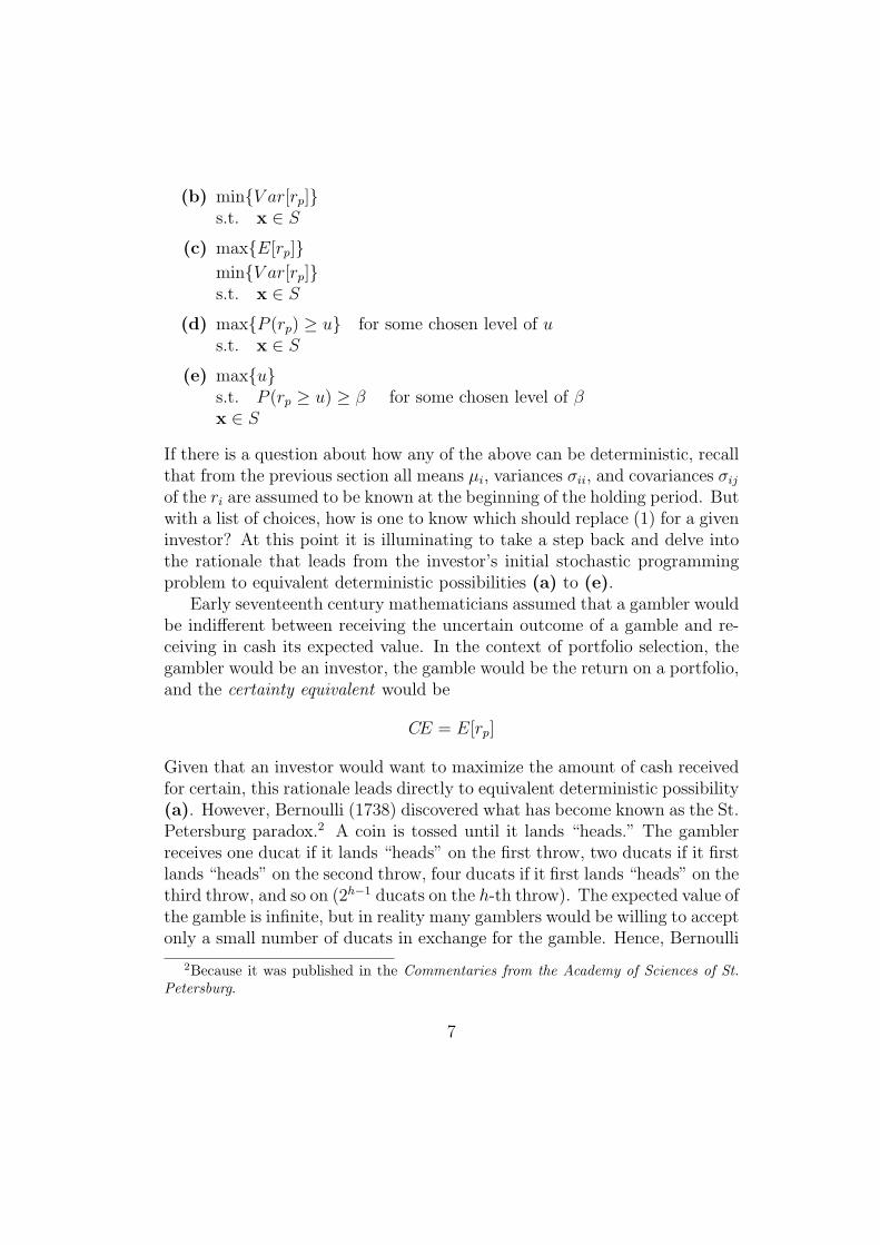
(b) min{V ar[rp]}s.t. x ∈ S

(c) max{E[rp]}min{V ar[rp]}s.t. x ∈ S

(d) max{P (rp) ≥ u} for some chosen level of us.t. x ∈ S

(e) max{u}s.t. P (rp ≥ u) ≥ β for some chosen level of βx ∈ S

If there is a question about how any of the above can be deterministic, recallthat from the previous section all means µi, variances σii, and covariances σij

of the ri are assumed to be known at the beginning of the holding period. Butwith a list of choices, how is one to know which should replace (1) for a giveninvestor? At this point it is illuminating to take a step back and delve intothe rationale that leads from the investor’s initial stochastic programmingproblem to equivalent deterministic possibilities (a) to (e).

Early seventeenth century mathematicians assumed that a gambler wouldbe indifferent between receiving the uncertain outcome of a gamble and re-ceiving in cash its expected value. In the context of portfolio selection, thegambler would be an investor, the gamble would be the return on a portfolio,and the certainty equivalent would be

CE = E[rp]

Given that an investor would want to maximize the amount of cash receivedfor certain, this rationale leads directly to equivalent deterministic possibility(a). However, Bernoulli (1738) discovered what has become known as the St.Petersburg paradox.2 A coin is tossed until it lands “heads.” The gamblerreceives one ducat if it lands “heads” on the first throw, two ducats if it firstlands “heads” on the second throw, four ducats if it first lands “heads” on thethird throw, and so on (2h−1 ducats on the h-th throw). The expected value ofthe gamble is infinite, but in reality many gamblers would be willing to acceptonly a small number of ducats in exchange for the gamble. Hence, Bernoulli

2Because it was published in the Commentaries from the Academy of Sciences of St.Petersburg.

7

suggested not to compare cash outcomes, but to compare the “utilities” ofcash outcomes. With the utility of a cash outcome given by a U : R → R,we thus have

U(CE) = E[U(rp)]

That is, the utility of CE equals the expected utility of the uncertain portfolioreturn.

With an investor wishing to maximize U(CE), this leads to the problemof Bernoulli’s principle of maximum expected utility

max{E[U(rp)]} (2)

s.t. x ∈ S

With U obviously increasing with rp, this means that any x that solves (2)solves (1), and vice versa. Although Bernoulli’s maximum expected utilityproblem (2) is a deterministic equivalent to (1), we call it an equivalent “un-determined” deterministic problem. This is because it is not fully determinedin that it contains unknown utility function parameters and cannot be solvedin its present form. However, with investors assumed to be risk averse, (i.e.,the expected value E[rp] is always preferred over the uncertain outcome rp),we at least know that in (2) U is concave.

Two schools of thought have evolved for dealing with the undeterminednature of U . One, in the spirit of Roy, involves attempting to ascertainaspects of an investor’s preference structure for the purpose of using themto solve (2) directly for an optimal portfolio. The other, in the spirit ofMarkowitz, involves parameterizing U and then attempting to solve (2) forall possible values of its unknown parameters. With this at the core of con-temporary portfolio theory, Markowitz considered a parameterized quadraticutility function3

U(x) = x− (λ/2)x2 (3)

Since U(x) above is normalized such that U(0) = 0 and U ′(0) = 1, this leavesexactly one parameter λ, the coefficient of risk aversion. By this parameteri-zation, Markowitz showed that precisely all potentially maximizing solutions

3There is an anomaly with quadratic utility functions since they decrease from a certainpoint on. Instead of quadratic utility, an alternative argument (not shown) leading tothe same result can be made by assuming that U is concave and increasing, and thatr = (r1, . . . , rn) follows a multinormal distribution.

8

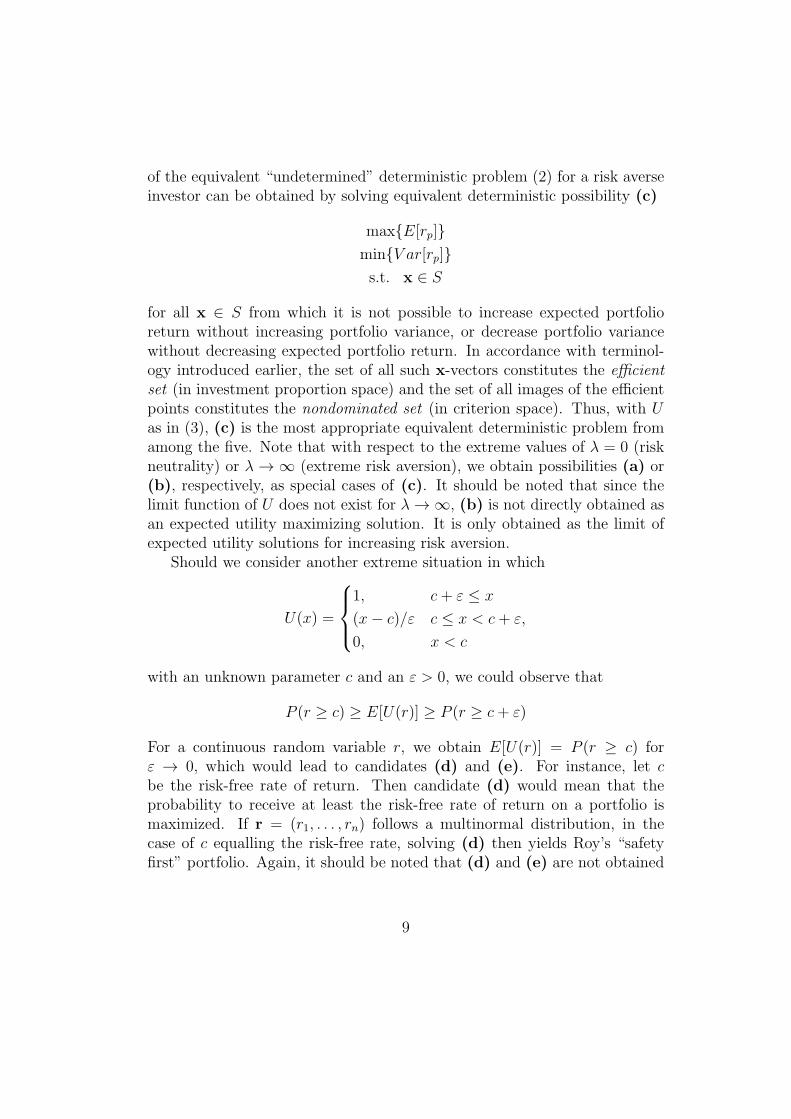
of the equivalent “undetermined” deterministic problem (2) for a risk averseinvestor can be obtained by solving equivalent deterministic possibility (c)

max{E[rp]}min{V ar[rp]}s.t. x ∈ S

for all x ∈ S from which it is not possible to increase expected portfolioreturn without increasing portfolio variance, or decrease portfolio variancewithout decreasing expected portfolio return. In accordance with terminol-ogy introduced earlier, the set of all such x-vectors constitutes the efficientset (in investment proportion space) and the set of all images of the efficientpoints constitutes the nondominated set (in criterion space). Thus, with Uas in (3), (c) is the most appropriate equivalent deterministic problem fromamong the five. Note that with respect to the extreme values of λ = 0 (riskneutrality) or λ → ∞ (extreme risk aversion), we obtain possibilities (a) or(b), respectively, as special cases of (c). It should be noted that since thelimit function of U does not exist for λ → ∞, (b) is not directly obtained asan expected utility maximizing solution. It is only obtained as the limit ofexpected utility solutions for increasing risk aversion.

Should we consider another extreme situation in which

U(x) =

1, c+ ε ≤ x

(x− c)/ε c ≤ x < c+ ε,

0, x < c

with an unknown parameter c and an ε > 0, we could observe that

P (r ≥ c) ≥ E[U(r)] ≥ P (r ≥ c+ ε)

For a continuous random variable r, we obtain E[U(r)] = P (r ≥ c) forε → 0, which would lead to candidates (d) and (e). For instance, let cbe the risk-free rate of return. Then candidate (d) would mean that theprobability to receive at least the risk-free rate of return on a portfolio ismaximized. If r = (r1, . . . , rn) follows a multinormal distribution, in thecase of c equalling the risk-free rate, solving (d) then yields Roy’s “safetyfirst” portfolio. Again, it should be noted that (d) and (e) are not obtained

9

as expected utility maximizing solutions4, but only as the limit of expectedutility solutions for an increasing focus on c.

Although not mentioned in Caballero, Cerda, Munoz, Rey and Stancu-Minasian, a sixth equivalent deterministic possibility stemming from (1) is

(f) max{E[rp]}min{V ar[rp]}max{Skew[rp]}s.t. x ∈ S

where Skew stands for skewness. With criterion vectors of length three,(f) is a multiple criteria portfolio selection problem. This formulation isprobably the only multiple criteria formulation that is not totally unfamiliarto conventional portfolio selection as a result of the interest taken in skewnessby authors such as Stone (1973), Konno and Suzuki (1995), Chunhachinda,Dandapani, Hamid and Prakash (1997), Prakash, Chang and Pactwa (2003).However, we will not dwell on (f) as this formulation, as a result of thesevere nonlinearities of its third criterion, has not gained much traction inpractice. Instead, we will concentrate on the newer types of multiple criteriaportfolio selection problems that have begun to appear as a result of themore sophisticated purposes of many investors.

4 Portfolio Selection with Multiple-Argument

Utility Functions

Whereas multiple criteria formulations are little more than a curiosity inconventional portfolio selection, multiple criteria formulations are mostlyappropriate when attempting to meet the modeling needs of investors withmultiple-argument utility functions. Two situations in which multiple-argumentutility functions are likely to occur are as follows.

One is that in addition to portfolio return, an investor has other consider-ations, such as to maximize social responsibility or to minimize the numberof securities in a portfolio, that are also important to the investor. That is,instead of being interested in solely maximizing the stochastic objective of

4While the limit function of U does exist for ε → 0, it contradicts the Archimedeanaxiom of von Neumann and Morgenstern (1947), i.e. the function is discontinuous.

10

portfolio return, the investor can be viewed as being interested in optimizingsome combination of several stochastic and several deterministic objectives.

A second situation in which a multiple-argument utility function mightpertain is when an investor is unwilling to accept the assumption that allmeans µi, variances σii, and covariances σij can be treated as known at thebeginning of the holding period. In response, an investor might wish tomonitor the construction of his or her portfolio with the help of additionalmeasures such as dividends, growth in sales, amount invested in R&D, andso forth, to guard against relying on any single measure that might haveimperfections associated with it.

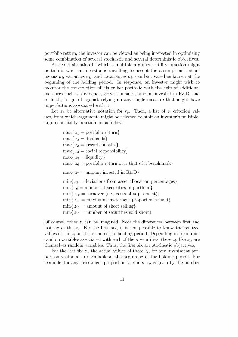
Let z1 be alternative notation for rp. Then, a list of zi criterion val-ues, from which arguments might be selected to staff an investor’s multiple-argument utility function, is as follows.

max{ z1 = portfolio return}max{ z2 = dividends}max{ z3 = growth in sales}max{ z4 = social responsibility}max{ z5 = liquidity}max{ z6 = portfolio return over that of a benchmark}

max{ z7 = amount invested in R&D}

min{ z8 = deviations from asset allocation percentages}min{ z9 = number of securities in portfolio}min{ z10 = turnover (i.e., costs of adjustment)}min{ z11 = maximum investment proportion weight}min{ z12 = amount of short selling}min{ z13 = number of securities sold short}

Of course, other zi can be imagined. Note the differences between first andlast six of the zi. For the first six, it is not possible to know the realizedvalues of the zi until the end of the holding period. Depending in turn uponrandom variables associated with each of the n securities, these zi, like z1, arethemselves random variables. Thus, the first six are stochastic objectives.

For the last six zi, the actual values of these zi, for any investment pro-portion vector x, are available at the beginning of the holding period. Forexample, for any investment proportion vector x, z9 is given by the number

11

of nonzero components in x. With the last six zi known in this way at thebeginning of the holding period, they are deterministic objectives.

As for z7 in the middle, it is an example of a measure that could be arguedeither way. It could be argued that only the most recent amounts investedin R&D are relevant to the situation at the end of the holding period, thusenabling the objective to be treated deterministically.

One might ask why can’t extra objectives be handled by means of con-straints? The difficulty is in the setting of the right-hand sides of the con-straints. In general, for a model to produce a mean-variance nondominatedfrontier that contains the criterion vector of an optimal portfolio, one wouldneed to know the optimal value of each objective modeled as a constraintprior to computing the frontier. It is not likely that this would be possiblein many situations.

With z1 almost certainly an argument of every investor’s utility function,additional arguments depend upon the investor. For instance, one investor’sset of arguments might consist of {z1, z2, z10}, and another’s might consist of{z1, z5, z7, z8, z11}. The point is that all investors need not be the same. Ifwe let k be the number of selected objectives, in the case of the first investor,k = 3, and in the case of the second investor, k = 5. Of course, a conventionalmean-variance investor’s set of arguments would only be {z1} in which casek = 1.

The differences between conventional portfolio selection and multiple cri-teria portfolio selection are highlighted in Figures 1 and 2. At the top ofeach, as in Saaty’s Analytic Hierarchy Process (1999), is the investor’s over-all focus. In Figure 1, the overall focus is to maximize the portfolio returnrandom variable. In Figure 2, the overall focus is to optimize some combina-tion of stochastic and deterministic objectives. In the second box of each isthe investor’s initial stochastic programming problem. Note that the initialstochastic programming problem in Figure 2 reflects the multiple stochasticand deterministic objectives involved in the investor’s overall focus and henceis a multiobjective stochastic program. As for notation in the second, thirdand fourth boxes of Figure 2, η specifies the number of stochastic objectivesof concern and Diη+1(x) represents the first of the k− η deterministic objec-tives of concern. For instance, if D13(x) were included, then D13(x) wouldrepresent a function that returns the number of negative xi.

In the third box of Figure 2 is the equivalent “undetermined” determin-

12

maximize stochasticobjective of portfolio return

?

overall focus

max{z1}s.t. x ∈ S

?

initialstochasticprogram

max{E[U(z1)]}s.t. x ∈ S

?

“undetermined”deterministicprogram

max{E[z1]}min{V ar[z1]}s.t. x ∈ S

deterministicimplementation

program

Figure 1: Hierarchical structure of the overall focus, initial stochastic pro-gram, equivalent “undetermined” deterministic program, and equivalent de-terministic implementation program of conventional portfolio selection.

istic problem

max{E[U(zi1 , . . . , ziη , ziη+1 , . . . , zik)]} (4)

s.t. x ∈ S

which shows the multiple-argument utility function that follows from theinvestor’s overall focus. Employing a mean-variance pair for each stochas-tic argument of the utility function, we have the equivalent deterministicimplementation program of the bottommost box. We use the term “imple-mentation” because this is the actual deterministic problem that is imple-mented. Note that all deterministic objectives of the initial (multiobjective)stochastic program are repeated unchanged in the equivalent deterministicimplementation program.

As a practical matter, for stochastic objectives in which variation is smallor not of noteworthy importance, it may be possible to represent them in theequivalent deterministic implementation program of the bottommost box ofFigure 2 by (a) instead of (c). This would be very advantageous when

13

optimize some combination ofstochastic and deterministic objectives

?

overall focus

max{zi1}:

min{Diη+1(x)}:

s.t. x ∈ S

?

initial (multiobjective)stochasticprogram

max{E[U(zi1 , . . . , ziη , ziη+1 , . . . , zik)]}s.t. x ∈ S

?

“undetermined”deterministicprogram

max{E[zi1 ]}min{V ar[zi1 ]}

:min{Diη+1(x)}

:s.t. x ∈ S

deterministicimplementation

program

Figure 2: Hierarchical structure of the overall focus, initial (multiobjective)stochastic program, equivalent “undetermined” deterministic program, andequivalent deterministic implementation program of multiple criteria portfo-lio selection

possible. For example, suppose an investor’s set is {z1, z2, z5}. Since theseobjectives are linear in the portfolio weights. the investor’s initial (multiob-

14

jective) stochastic program would be

max{ z1 =n∑

j=1

rjxj}

max{ z2 =n∑

j=1

djxj}

max{ z5 =n∑

j=1

ℓjxj}

s.t. x ∈ S

in which dj is the random variable for the dividends, and ℓj is the randomvariable for the liquidity, of the j-th security. Should variations in portfoliodividends and portfolio liquidity be much less important than variations inportfolio return, then it may well be acceptable to use (a) instead of (c) foreach of dividends and liquidity. Then the resulting equivalent deterministicimplementation program would be

max{E[z1]} (5)

min{V ar[z1]}max{E[z2]}max{E[z5]}s.t. x ∈ S

The advantage of being able to use (a) instead of (c) with stochastic objec-tives beyond portfolio return is of course that a V ar objective for each suchobjective can be eliminated from the equivalent deterministic implementa-tion program. This not only simplifies data collection requirements (as it isonly necessary to know the means of the relevant random variables), but alsolessens the burden on computing the nondominated set.

5 Mean-Variance Nondominated Sets

We now utilize matrix notation when convenient. To prepare for the ap-plication of the four stages of the Markowitz solution procedure to multiple

15

criteria portfolio selection problems, it is useful to study in a little greaterdetail the mean-variance formulation in the bottommost box of Figure 1

max{E[z1] = µTx} (6)

min{V ar[z1] = xTΣx }s.t. x ∈ S

in which µ ∈ Rn is the expected value vector of the ri and Σ ∈ Rn×n

is the covariance matrix of the σij. In this problem, the efficient set is apiecewise linear path in S. The nondominated set, being the set of imagesof all efficient points, is piecewise parabolic in (V ar[z1], E[z1]) space. Thismeans that when portrayed in (Stdev[z1], E[z1]) space, the nondominated setis piecewise hyperbolic. Although theory and computation are customarilycarried out in (V ar[z1], E[z1]) space, we mention (Stdev[z1], E[z1]) space asmost nondominated sets are communicated to investors in this space.

When the feasible region is the 1Tx = 1 hyperplane as in

S = {x ∈ Rn | 1Tx = 1 } (7)

the efficient and nondominated sets are straightforward. The efficient set is a(single) straight line in the hyperplane, bounded at one end and unbounded atthe other. The nondominated set is the top half of a (single) hyperbola. And,as a consequence of the 1Tx = 1 nature of S, the efficient and nondominatedsets can, after taking the Lagrangian, be obtained by formula (see for instanceCampbell, Lo and Mackinlay (1997)).

However, as soon as additional constraints become involved as in

S = {x ∈ Rn | 1Tx = 1, αi ≤ xi ≤ ωi} (8)

thereby making S a subset of the 1Tx = 1 hyperplane, the situation becomesmore complicated. To illustrate, consider Figure 3 (which might correspondto a problem with about 8 securities). With a little poetic license mandatedby the fact that it is not possible to draw a graph in 8-space, the graph on theleft is intended to portray (a) the subset of the 1Tx = 1 hyperplane that isS and (b) the efficient set which is normally a piecewise linear path. On theright in (Stdev[z1], E[z1]) space is the nondominated set (or frontier). Corre-sponding to the five segments of the piecewise linear path, the nondominatedfrontier consists of five hyperbolic segments. Note that the inverse images

16

x1

x3

x2

x4

x5x

6

z1

z6

z5

z4

z3

z2

.

. .

.

Stdev[z1]

E[z1]

Figure 3: Piecewise linear efficient set in S (left) and piecewise hyperbolicnondominated set in (Stdev[z1], E[z1]) space (right)

of the endpoints of a given nondominated hyperbolic segment are the end-points of the efficient line segment that generates the hyperbolic segment.For instance, the inverse images of z1 and z2 are x1 and x2, respectively.

A property of a nondominated hyperbolic segment is that along the seg-ment excluding its endpoints, the securities in a portfolio remain the same.Only their proportions change as we move along the segment. Securitiescan only leave a nondominated portfolio at an endpoint, and securities canonly enter a nondominated portfolio if we cross over an endpoint (such asz2) to an adjacent nondominated hyperbolic segment. As for the number ofnondominated hyperbolic segments, the larger the problem, the greater thenumber of nondominated hyperbolic segments. For instance, a problem with100 securities might have 30 to 60 nondominated hyperbolic segments. Apartfrom when S is the entire 1Tx = 1 hyperplane, mathematical programmingis now the tool for obtaining information about efficient and nondominatedsets.

What about software? In the past there was the IBM (1965) code. Earlycomputer codes suffered from two problems. One was speed and the otherwas core (i.e., memory). Because of the amount of core required for storinga dense covariance, methods for “sparsifying” or “simplifying” the covari-ance matrix structure all but dominated portfolio optimization research forthe next twenty years. Also, there was debate about whether a portfoliocode should be “parametric” or “one-at-a-time.” A parametric code is one

17

that is able to define the nondominated frontier as a function of some sin-gle parameter. A one-at-a-time code simply computes points, one-at-a-time,on the nondominated frontier, for instance, by repetitively solving the “e-constraint” formulation5

min{xTΣx} (9)

s.t. µTx ≥ ρ

x ∈ S

for different values of ρ. Then, with the points obtained, representations ofthe nondominated frontier as in Figure 4 can be prepared.

In the 1980s there was the Perold code. For achieving a breaktroughwith large-scale problems (500 securities was considered large scale at thetime), the code was predicated upon a covariance matrix structure sparsifiedaccording to the techniques in Markowitz and Perold (1981a and 1981b) andPerold (1984). Algorithmically drawing upon Markowitz (1956), the code wasnot one-at-a-time, but parametric as it was able to compute parametricallythe nondominated frontier. Having been programmed on older platforms,neither the IBM code nor Perold’s code is any longer in distribution. Apaper describing latest developments in portfolio optimization up until theearly mid 90s is by Pardalos, Sandstrom and Zopounidis (1994)

As for currently, the situation is eclectic. One one hand, there are “propri-etary systems” which are not really intended for university use. Rather, theyare intended for integration into the computing systems of (mainly large)firms in the financial services industry. Depending upon the modificationsnecessary to fit into a client’s computer system, the number of users, andthe amount of training involved, such systems can easily run into the tens ofthousands of dollars. Two such proprietary systems are FortMP, as alludedto in Mitra, Kyriakis, Lucas and Pirbhai (2003)), and QOS developed outof the works of Best (1996), Best and Kale (2000), and Best and Hlouskova(2005). Each with its own features, they are designed for large-scale problemsand perform at high speed. However, they do not parametrically specify thenondominated frontier. Rather they compute points on the nondominatedfrontier thus resulting in both being classified as one-at-a-time.

As for codes more suitable for university use, there is the public domaincode Optimizer given in the appendix of Markowitz and Todd (2000). Opti-

5In multiple criteria optimization, programs with all objectives but one converted toconstraints are often called e-constraint formulations.

18

.

.

.

Figure 4: Dotted (left) and piecewise linear (right) representations of a non-dominated frontier

mizer is parametric as it implements the critical line algorithm of Markowitz(1956). It is written in VBA (Visual Basic for Applications). However, as ofthis writing, it is limited to 248 securities.

One might think that commands for computing the linear segments ofthe efficient set and the hyperbolic segments of the nondominated frontierof (6) would be included in packages such as Cplex, Mathematica, Matlab,LINGO, SAS, and premium versions of Solver, but this is not the case. Otherthan for the simplistic case when S is the 1Tx = 1 hyperplane, the best thatcan be done with the packages is to write routines within them to computepoints on the nondominated frontier utilizing formulations such as (9), thusconsigning us, with the packages, to an essentially one-at-a-time world.

6 Solving a Multiple Criteria Portfolio Selec-

tion Problem

Building upon knowledge gained in the previous section, we are now ableto discuss the task of solving a multiple criteria portfolio selection problem.While the protocol of computing the nondominated set, communicating itto the investor, searching the nondominated set for a most preferred point,and then taking an inverse image of the selected point still remains intact,the first three stages present much greater difficulties. As for the equivalent

19

deterministic implementation program of the bottommost box of Figure 2,different types of formulations may result. For purposes of discussion, wedivide them into the three categories: (1) those with one quadratic and twoor more linear objectives, (2) those with two or more quadratic and one ormore linear objectives, and (3) those with one or more non-smooth objectivefunctions (for instance D9(x), which is to minimize the number of securities,is non-smooth).

6.1 One Quadratic and Two or More Linear Objectives

Although many of the problems that can emerge in the bottommost box ofFigure 2 cannot, given where we are in the development of multiple crite-ria portfolio selection, yet be effectively addressed, progress is being madeon 1-quadratic 2-linear and 1-quadratic 3-linear problems in Hirschberger,Qi and Steuer (2007), and on this we comment. For instance, whereas thenondominated frontier of a mean-variance problem is piecewise hyperbolicin (Stdev[z1], E[z1]) space, the nondominated set (surface) of a 1-quadraticmulti-linear multiple criteria portfolio selection is platelet-wise hyperboloidicin (Stdev[z1], E[z1], E[z2], . . .) space. That is, the nondominated set is com-posed of patches, with each patch coming from the surface of a differenthyperboloid. Also, whereas the efficient set in the mean-variance case is apath of linear line segments, the efficient set of a 1-quadratic multi-linearproblem is a connected union of low-dimensional polyhedra in S.

Stdev[z1]

za

zd

zbE[z1]

E[z2]

zc

Figure 5: Efficient set in S (left) and platelet-wise hyperboloidic nondomi-nated set of a 1-quadratic 2-linear multiple criteria portfolio selection problemin (Stdev[z1], E[z1], E[z2]) space (right)

20

Consider Figure 5. On the left, the efficient set is portrayed showing thepolyhedral subsets of which it is composed. On the right, the nondominatedset is portrayed showing the hyperboloidic platelets of which it is composed.Note that not all platelets are of the same size and that they generally de-crease in size the closer we are to the minimum standard deviation point.This is normal. Also, it is normal for not all platelets to have the samenumber of (platelet) corner points. Note the correspondence between thenondominated hyperboloidic platelets and the efficient polyhedral subsets.For instance, the platelet defined by corner points za, zb, zc, zd would beassociated with a polyhedral subset such as the shaded one with four ex-treme points on the left. And as in the mean-variance case, all portfolios inthe relative interior of a platelet contain the same securities, just in differentproportions, and for a security to leave or for a new one to enter, one wouldneed to cross the boundary to another platelet.

With regard to computing the nondominated set, we are able to reportlimited computational results using a code under development in Hirschberger,Qi and Steuer (2007). The results obtained are for 1-quadratic 2-linear prob-lems whose covariance matrices are 100% dense. With n = 200 securities, 1-quadratic 2-linear problems were found to have in the neighborhood of aboutone thousand nondominated platelets, taking on average about ten secondsto compute. The computer used was a Dell 2.13GHz Pentium M Centrinolaptop. With n = 400 securities, 1-quadratic 2-linear problems were foundto have in the neighborhood of about two thousand nondominated platelets,taking on average about one minute to compute. These are encouragingresults leading us to believe that the nondominated sets of larger problems(either in terms of number of securities or number of linear objectives) arecomputable in reasonable time.

Unfortunately, it is not as easy to display the nondominated set in mul-tiple criteria portfolio selection as in mean-variance portfolio selection. Inproblems with criterion vectors of length three, 3D graphics can be used, butin problems with more objectives, probably about the best that can be doneis to enable the investor to learn about the nondominated set while in theprocess of searching for a most preferred point.

As for searching the nondominated set of a problem such as in Figure 5,one approach is to discretize the nondominated set to some desired level ofresolution. This can be accomplished as follows. For each polyhedral subsetof the efficient set, take convex combinations of its extreme points. Becauseplatelet size tends to increase the more distant the platelet is from the min-

21

imum standard deviation point, one would probably want to increase thenumber of convex combinations the further the platelet is away. Then withperhaps tens of thousands, if not hundreds of thousands, of nondominatedpoints generated in this way, the question is how to locate a most preferred.Four strategies come to mind. One is to employ interactive multiple probingas in the Tchebycheff Method described in Steuer, Silverman and Whisman(1993). Another is to pursue a projected line search strategy as in Korhonenand Wallenius (1988) and Korhonen and Karaivanova (1999). A third is toutilize an interactive criterion vector component classification scheme as, forinstance, in Miettinen (1999). And a fourth might involve the utilizationof some of the visualization techniques described in Lotov, Bushenkov andKamenev (2004).

6.2 Two or More Quadratic and One or More LinearObjectives

To illustrate what can be done in this category, consider the 2-quadratic2-linear problem

min{xTΣ1 x } (10)

min{xTΣ2 x }max{µTx}max{νTx}s.t. x ∈ S

where Σ1 and Σ2 are positive definite and S is defined, for instance, as in(8). Given that Σ1 and Σ2 are positive definite, any convex combination

Σ = λΣ1 + (1− λ)Σ2

(where λ ∈ [0, 1]) renders Σ positive definite. This means that the nondom-inated set of the 1-quadratic 2-linear

min{xT Σ x } (11)

max{µTx}max{νTx}s.t. x ∈ S

22

is a subset of the nondominated set of (10). Thus, by solving (11) for aseries of different λ-values, we should be able to obtain a covering of thenondominated set of the original 2-quadratic 2-linear. The covering can thenbe handled in the same way as in the previous subsection.

6.3 One or More Non-Smooth Objectives

When a multiobjective equivalent deterministic problem possesses a non-smooth objective (such as to minimize the number of securities), we facemajor difficulties in that the problem is no longer continuous. Moreover,the nonpositive hull of the nondominated set might not even be convex. Inaddition, a problem might possess non-smooth constraints, for instance, inthe form of semi-continuous variables (variables that are either zero or insome interval [a, b] where a is materially greater than zero). Possibly, theonly way to attack such problems is to utilize evolutionary algorithms suchas set forth in Deb (2001).

7 Conclusions

For investors with additional concerns, portfolio selection need not only belooked at within a mean-variance framework. Steps can now be taken tointegrate additional concerns into the portfolio optimization process morein accordance with their criterion status. Instead of attempting to interjectadditional concerns into portfolio selection by means of constraints – an adhoc process that often ends prematurely because of losses in user patience –the methods that have been outlined form the basis for a new era of solutionmethodologies whose purposes are to converge to a final portfolio that moreformally achieves optimal trade-offs among all of the criteria that the in-vestor wishes to deem important. Of course, as with any area that is gainingmomentum, more work needs to be done.

References

[1] B. Aouni, F. Ben Abdelaziz, and R. El-Fayedh. Chance constrainedcompromise programming for portfolio selection. Laboratoire LARO-DEC, Institut Superieur de Gestion, La Bardo 2000, Tunis, Tunisia,2005.

23

[2] M. Arenas Parra, A. Bilbao Terol, and M. V. Rodrıguez Urıa. A fuzzygoal programming approach to portfolio selection. European Journal ofOperational Research, 133(2):287–297, 2001.

[3] E. Ballestero. Using compromise programming in a stock market pricingmodel. In Y. Y. Haimes and R. E. Steuer, editors, Lecture Notes in Eco-nomics and Mathematical Systems, vol. 487, pages 388–399. Springer-Verlag, Berlin, 2002.

[4] E. Ballestero and D. Pla-Santamarıa. Selecting portfolios for mutualfunds. Omega, 32:385–394, 2004.

[5] E. Ballestero and C. Romero. Portfolio selection: A compromiseprogramming solution. Journal of the Operational Research Society,47(11):1377–1386, 1996.

[6] C. A. Bana e Costa and J. O. Soares. Multicriteria approaches forportfolio selection: An overview. Review of Financial Markets, 4(1):19–26, 2001.

[7] C. A. Bana e Costa and J. O. Soares. A multicriteria model for portfoliomanagement. European Journal of Finance, 10(3), 2004. 198-211.

[8] D. Bernoulli. Specimen theoria novae de mensura sortis. CommentariiAcademiae Scientarum Imperialis Petropolitnae, 5(2):175–192, 1738.Translated into English by L. Sommer, Exposition of a new theory onthe measurement of risk, Econometrica, 22(1): 23-26, 1954.

[9] M. J. Best. An algorithm for the solution of the parametric quadraticprogramming problem. In B. Riedmuller H. Fischer and S. Schaffler,editors, Applied Mathematics and Parallel Computing: Festschrift forKlaus Ritter, pages 57–76. Physica-Verlag, 1996.

[10] M. J. Best and J. Hlouskova. An algorithm for portfolio optimizationwith transaction costs. Management Science, 51(11):1676–1688, 2005.

[11] M. J. Best and J. Kale. Quadratic programming for large-scale port-folio optimization. In J. Keyes, editor, Financial Services InformationSystems, pages 513–529. CRC Press, 2000.

24

[12] G. Bouri, J. M. Martel, and H. Chabchoub. A multi-criterion approachfor selecting attractive portfolio. Journal of Multi-Criteria DecisionAnalysis, 11(3):269–277, 2002.

[13] R. Caballero, E. Cerda, M. M. Munoz, L. Rey, and I. M. Stancu-Minasian. Efficient solution concepts and their relations in stochasticmultiobjective programming. Journal of Optimization Theory and Ap-plications, 110(1):53–74, 2001.

[14] J. Y. Campbell, A. W. Lo, and A. C. Mackinlay. The Econometrics ofFinancial Markets. Princeton University Press, Princeton, New Jersey,1997.

[15] G. Chow. Portfolio selection based on return, risk, and relative perfor-mance. Financial Analysts Journal, pages 54–60, March-April 1995.

[16] P. Chunhachinda, K. Dandapani, S. Hamid, and A. J. Prakash. Port-folio selection and skewness evidence from international stock markets.Journal of Banking & Finance, 21:143–167, 1997.

[17] G. Colson and Ch. DeBruyn. An integrated multiobjective portfoliomanagement system. Mathematical and Computer Modelling, 12(10-11):1359–1381, 1989.

[18] K. Deb. Multi-Objective Optimization using Evolutionary Algorithms.John Wiley, New York, 2001.

[19] C. Dominiak. An application of interactive multiple objective goal pro-gramming on the Warsaw stock exchange. In R. Caballero, F. Ruiz, andR. E. Steuer, editors, Lecture Notes in Economics and MathematicalSystems, vol. 455, pages 66–74. Springer-Verlag, Berlin, 1997.

[20] C. Dominiak. Portfolio selection using the idea of reference solution. InG. Fandel and T. Gal, editors, Lecture Notes in Economics and Mathe-matical Systems, vol. 448, pages 593–602. Springer-Verlag, Berlin, 1997.

[21] M. Doumpos, M. Spanos, and C. Zopounidis. On the use of goal pro-gramming techniques in the assessment of financial risks. Journal ofEuro-Asian Management, 5(1):83–100, 1999.

25

[22] M. Ehrgott, K. Klamroth, and C. Schwehm. An MCDM approachto portfolio optimization. European Journal of Operational Research,155(3):752–770, 2004.

[23] E. J. Elton, M. J. Gruber, S. J. Brown, and W. Goetzmann. ModernPortfolio Theory and Investment Analysis. John Wiley, New York, 6thedition, 2002.

[24] J. Fliege. Gap-free computation of Pareto-points by quadratic scalar-izations. Mathematical Methods of Operations Research, 59(1):69–89,2004.

[25] W. G. Hallerbach and J. Spronk. A multidimensional framework forfinancial-economic decisions. Journal of Multi-Criteria Decision Analy-sis, 11(3):111–124, 2002.

[26] W. G. Hallerbach and J. Spronk. The relevance of MCDM for financialdecisions. Journal of Multi-Criteria Decision Analysis, 11(4-5):187–195,2002.

[27] M. Hirschberger, Y. Qi, and R. E. Steuer. Tri-criterion quadratic-linearprogramming. In-preparation working paper, Department of Bankingand Finance, University of Georgia, Athens, 2007.

[28] Ch. Hurson and C. Zopounidis. On the use of multi-criteria decisionaid methods to portfolio selection. Journal of Euro-Asian Management,1(2):69–94, 1995.

[29] IBM. “1401 Portfolio Selection Program (1401-F1-04X) Program Ref-erence Manual,” IBM, New York, 1965.

[30] P. Kliber. “A three-criteria portfolio selection: mean return, risk andcosts of adjustment,” Akademia Ekonomiczna w Poznaniu, Poznan,Poland, 2005.

[31] H. Konno, H. Shirakawa, and H. Yamazaki. A mean-absolute deviation-skewness portfolio optimization model. Annals of Operations Research,45:205–220, 1993.

[32] H. Konno and K.-I. Suzuki. A mean-variance-skewness portfolio opti-mization model. Journal of the Operations Research Society of Japan,38(2):173–187, 1995.

26

[33] P. Korhonen and J. Karaivanova. An algoithm for projecting a referencedirection onto the nondominated set of given points. IEEE Transactionson Systems, Man, and Cybernetics, 29(5):429–435, 1999.

[34] P. Korhonen and J. Wallenius. A Pareto Race. Naval Research Logistics,35(6):615–623, 1988.

[35] P. Korhonen and G.-Y. Yu. A reference direction approach to multipleobjective quadratic-linear programming. European Journal of Opera-tional Research, 102(3):601–610, 1997.

[36] S. M. Lee and A. J. Lerro. Optimizing the portfolio selection for mutualfunds. Journal of Finance, 28(5):1087–1101, 1973.

[37] H. L’Hoir and J. Teghem. Portfolio selection by MOLP using interactivebranch and bound. Foundations of Computing and Decision Sciences,20(3):175–185, 1995.

[38] A. W. Lo, C. Petrov, and M. Wierzbicki. It’s 11pm – Do you knowwhere your liquidity is? The mean-variance-liquidity frontier. Journalof Investment Management, 1(1):55–93, 2003.

[39] A. B. Lotov, V. A. Bushenkov, and G. K. Kamenev. Interactuve DecisionMaps: Approximation and Visualization of Pareto Frontier. KluwerAcademic Publishers, Boston, 2004.

[40] H. M. Markowitz. Portfolio selection. Journal of Finance, 7(1):77–91,1952.

[41] H. M. Markowitz. The optimization of a quadratic function subject tolinear constraints. Naval Research Logistics Quarterly, 3:111–133, 1956.

[42] H. M. Markowitz. The early history of portfolio selection: 1600-1960.Financial Analysts Journal, pages 5–16, July 1999.

[43] H. M. Markowitz and A. Perold. Portfolio analysis with factors andscenarios. Journal of Finance, 36(14):871–877, 1981a.

[44] H. M. Markowitz and A. Perold. Sparsity and piecewise linearity in largescale portfolio optimization problems. In I. Duff, editor, Sparse Matri-ces and Their Use, (The Institute of Mathematics and Its ApplicationsConference Series), pages 89–108. Academic Press, New York, 1981b.

27

[45] H. M. Markowitz and G. P. Todd. Mean-Variance Analysis in PortfolioChoice and Capital Markets. Frank J. Fabozzi Associates, New Hope,Pennsylvania, 2000.

[46] K. M. Miettinen. Nonlinear Multiobjective Optimization. Kluwer,Boston, 1999.

[47] G. Mitra, T. Kyriakis, C. Lucas, and M. Pirbhai. A review of portfolioplanning: models and systems. In S. E. Satchell and A. E. Scowcroft,editors, Advances in Portfolio Construction and Implementation, pages1–39. Butterworth-Heinemann, Oxford, 2003.

[48] W. Ogryczak. Multiple criteria linear programming model for portfolioselection. Annals of Operations Research, 97:143–162, 2000.

[49] P. M. Pardalos, M. Sandstrom, and C. Zopounidis. On the use of op-timization models for portfolio selection: A review and some computa-tional results. Computational Economics, 7(4):227–244, 1994.

[50] A. Perold. Large-scale portfolio optimization. Management Science,30(10):1143–1160, 1984.

[51] A. J. Prakash, C. H. Chang, and T. E. Pactwa. Selecting a portfolio withskewness: Recent evidence from US, European, and Latin Americanequity markets. Journal of Banking & Finance, 27:1375–1390, 2003.

[52] A. Prekopa. Stochastic Programming. Kluwer Academic Publishers,Dordrecht, 1995.

[53] A. D. Roy. Safety first and the holding of assets. Econometrica,20(3):431–449, 1952.

[54] T. L. Saaty. Decision Making for Leaders. RWS Publications, Pitts-burgh, 1999–2000 edition, 1999.

[55] R. Slowinski and J. Teghem, editors. Stochastic versus Fuzzy Ap-proaches to Multiobjective Mathematical Programming under Uncertain-tyd. Kluwer Academic Publishers, Dordrecht, Netherlands, 1990.

[56] J. Spronk. Interactive Multiple Goal Programming: Applications to Fi-nancial Management. Martinus Nijhoff Publishing, Boston, 1981.

28

[57] J. Spronk and W. G. Hallerbach. Financial modelling: Where to go?with an illustration for portfolio management. European Journal ofOperational Research, 99(1):113–127, 1997.

[58] J. Spronk, R. E. Steuer, and C. Zopounidis. Multicriteria decision anal-ysis/aid in finance. In J. Figuiera, S. Greco, and M. Ehrgott, editors,Multiple Criteria Decision Analysis: State of the Art Surveys, pages799–857. Springer Science, 2005.

[59] I. Stancu-Minasian. Stochastic Programming with Multiple-ObjectiveFunctions. D. Reidel Publishing Company, Dordrecht, Netherlands,1984.

[60] R. E. Steuer and P. Na. Multiple criteria decision making combined withfinance: A categorized bibliography. European Journal of OperationalResearch, 150(3):496–515, 2003.

[61] R. E. Steuer, Y. Qi, and M. Hirschberger. Multiple objectives in portfolioselection. Journal of Financial Decision Making, 1(1):5–20, 2005.

[62] R. E. Steuer, Y. Qi, and M. Hirschberger. Developments in multi-attribute portfolio selection. In T. Trzaskalik, editor, Multiple Crite-ria Decision Making ’05, pages 251–262. Karol Adamiecki University ofEconomics in Katowice, 2006.

[63] R. E. Steuer, Y. Qi, and M. Hirschberger. Suitable-portfolio investors,nondominated frontier sensitivity, and the effect of multiple objectiveson standard portfolio selection. Annals of Operations Research, 2006.forthcoming.

[64] R. E. Steuer, J. Silverman, and A. W. Whisman. A combined Tcheby-cheff/aspiration criterion vector interactive multiobjective programmingprocedure. Management Science, 39(10):1255–1260, 1993.

[65] B. K. Stone. A linear programming formulation of the general portfo-lio selection problem. Journal of Financial and Quantitative Analysis,8(4):621–636, 1973.

[66] M. Tamiz, R. Hasham, D. F. Jones, B. Hesni, and E. K. Fargher. A twostaged goal programming model for portfolio selection. In M. Tamiz,

29

editor, Lecture Notes in Economics and Mathematical Systems, vol. 432,pages 386–399. Springer-Verlag, Berlin, 1996.

[67] J. Xu and J. Li. A class of stochastic optimization problems with onequadratic & several linear objective functions and extended portfolioselection model. Journal of Computational and Applied Mathematics,146:99–113, 2002.

[68] G. Y. Yu. A multiple criteria approach to choosing an efficient stockportfolio at the Helsinki stock exchange. Journal of Euro-Asian Man-agement, 3(2):53–85, 1997.

[69] W. T. Ziemba. The Stochastic Programming Approach to Asset, Li-ability, and Wealth Management. Research Foundation of the AIMR,Charlottesville, Virginia, 2003.

30