Portfolio Choice and the Bayesian Kelly Criterion

Sid Browne 1

Columbia UniversityWard Whitt 2

AT&T Bell Laboratories

Original: March 4, 1994Final Version: August 3, 1995

Appeared in Advances in Applied Probability, 28, 4: 1145-1176, December 1996

1Postal address: 402 Uris Hall, Graduate School of Business, Columbia University, New York, NY 100272Postal address: AT&T Bell Laboratories, Room 2C-178, Murray Hill NJ 07974-0636

Abstract

We derive optimal gambling and investment policies for cases in which the underlying stochastic

process has parameter values that are unobserved random variables. For the objective of maximizing

logarithmic utility when the underlying stochastic process is a simple random walk in a random

environment, we show that a state-dependent control is optimal, which is a generalization of the

celebrated Kelly strategy: The optimal strategy is to bet a fraction of current wealth equal to a

linear function of the posterior mean increment. To approximate more general stochastic processes,

we consider a continuous-time analog involving Brownian motion. To analyze the continuous-time

problem, we study the diffusion limit of random walks in a random environment. We prove that

they converge weakly to a Kiefer process, or tied-down Brownian sheet. We then find conditions

under which the discrete-time process converges to a diffusion, and analyze the resulting process.

We analyze in detail the case of the natural conjugate prior, where the success probability has a beta

distribution, and show that the resulting limiting diffusion can be viewed as a rescaled Brownian

motion. These results allow explicit computation of the optimal control policies for the continuous-

time gambling and investment problems without resorting to continuous-time stochastic-control

procedures. Moreover they also allow an explicit quantitative evaluation of the financial value

of randomness, the financial gain of perfect information and the financial cost of learning in the

Bayesian problem.

Key words: betting systems; proportional gambling; Kelly criterion; portfolio theory; logarithmic

utility; random walks in a random environment; Kiefer process; time-changed Brownian motion;

conjugate priors; Bayesian control.

AMS 1991 Subject Classification: Primary: 90A09. Secondary: 60G40, 62C10, 60J60.

1 Introduction

Suppose you are faced with a sequence of favorable games, and you decide to bet repeatedly on

these games using proportional betting. If you bet x on the nth game, then your return is xZn,

where {Zn : n ≥ 1} is a sequence of i.i.d. random variables with EZn > 0. Let Vn be your fortune

after n bets, and let fn denote the proportion of your wealth that you wager on the nth bet. Your

fortune then evolves as

Vn = Vn−1 + (fnVn−1)Zn = Vn−1(1 + fnZn) = V0

n∏i=1

(1 + fiZi) , n ≥ 1 . (1)

Of considerable interest is the special case where you always bet the same constant proportion,

fn = f , for all n ≥ 1. For such a policy, let the growth rate of your strategy be defined by

Gn(f) ≡ 1

nln(Vn/V0) ≡

1

n

n∑i=1

ln(1 + fZi) .

By the Law of Large Numbers,

Gn(f)→ G(f) ≡ E(ln(1 + fZ1)) w.p.1 as n→∞ .

You can optimize your long-run growth rate by choosing f to maximize G(f); this is commonly

referred to as the Kelly criterion, and the resulting constant proportional strategy is commonly

referred to as the Kelly gambling scheme, in honor of the seminal paper by Kelly (1956). Pro-

portional betting or Kelly gambling has since been quite extensively studied; see Breiman (1961),

Thorp (1969), Bell and Cover (1980), Finkelstein and Whitely (1981), Ethier and Tavare (1983),

Ethier (1988), Algoet and Cover (1988) and Cover and Thomas (1991).

Kelly (1956) treated the special case in which Zn is the increment in a simple random walk, i.e.,

P (Zn = 1) = θ = 1− P (Zn = −1) .

For this case,

G(f) = θ ln(1 + f) + (1− θ) ln(1− f) ,

from which we see that the optimal fixed fraction is just the mean increment in the random walk

f∗ = 2θ − 1 = EZn (2)

and the optimal win rate is

G(f∗) = Λ(θ) := ln 2 + θ ln θ + (1− θ) ln(1− θ) , (3)

which is ln 2−H, where H is the entropy of the distribution of Z1.

For more general random walks, where Zn has an arbitrary distribution, it is clear that the

optimal policy is still f∗ = arg supf E(ln(1 + fZ1)), although computation of the optimal policy is

1

in general much more difficult. Some approximations to the optimal policy for discrete-time models

are developed in Ethier and Tavare (1983), Ethier (1988) and Thorp (1971).

It is now known that proportional betting has many good properties, besides maximizing the

growth rate. For example, Breiman (1961) proved that f∗ also asymptotically minimizes the ex-

pected time to reach a fixed fortune, and asymptotically dominates any other strategy. There are

optimality properties associated with this strategy for finite horizons as well. For example, Bell and

Cover (1980) proved that this strategy is also optimal in a game theoretic sense for finite horizons.

Bellman and Kalaba (1957) also considered the problem for a simple random walk over a finite

horizon and proved that this policy is optimal for the equivalent problem of maximizing the utility

of terminal wealth at any fixed terminal time, when the utility function is logarithmic. Proportional

gambling and the Kelly problem have also been considered directly in a continuous-time setting in

Pestien and Sudderth (1985), Gottlieb (1985) and Heath, Orey, Pestien and Sudderth (1987). In

the continuous-time model, the underlying random walk is replaced by a Brownian motion (with

given positive drift). Many of the discrete-time optimality properties of proportional gambling also

carry over into the continuous-time model as well.

The problem of optimal gambling in repeated favorable games is intimately related to the

problem of optimal multi-period investment in financial economics. The only essential difference in

fact is the option of investing in a risk free security that pays a nonstochastic interest rate r > 0.

We consider here the simple case in which there is only one risky stock available for investment.

In this case Zn denotes the return of the risky stock on day n, and if the investor decides to invest

a fraction fn of his wealth in the risky stock on day n, with the remainder of his wealth wealth

invested in the riskless security, then his fortune evolves as

Vn = Vn−1 [1 + r(1− fn) + fnZn] = V0

n∏i=1

[1 + r(1− fi) + fiZi] .

Thus, all our results, while stated mostly in the picturesque language of gambling, are in fact equally

applicable to investment problems. The Kelly criterion in this context (usually referred to as the

optimal-growth criterion) was studied in discrete-time in Latane (1959) and Hakansson (1970), and

in continuous-time in Merton (1990) and Karatzas (1989). An adaptive portfolio strategy that

performs asymptotically as well as the best constant proportion strategy, for an arbitrary sequence

of gambles, was introduced in Cover (1991) (see also Cover and Gluss (1986)) in discrete-time and

was extended to continuous-time in Jamishidian (1992).

In this paper, we consider the Bayesian version of both the discrete and continuous-time gam-

bling and investment problems; where certain parameters of the distribution of the increment of

the underlying stochastic process are unobserved random variables. As the underlying stochastic

process evolves, the investor observes the outcomes and thus obtains information as to the true

value of the stochastic parameters. The approach taken in this paper is to first solve the discrete-

time problem, and then use those results to solve the continuous-time problem by treating it as the

(diffusion) limit of the discrete-time problem.

2

We study first the discrete-time problem. What we would really like to do is treat the case

where Zn has a general distribution, as well as allow some weak dependence in the sequence

{Zn}. However, while the optimal policy for the general case turns out to be relatively easy

to characterize (see (25) below), explicit computation of the policy is even more difficult than for

the non-Bayesian case. There is one case where the policy can be explicitly calculated, and that

is the simple random walk with a random success probability, which is the generalization of the

original Kelly (1956) problem. For this case, the optimal (Bayesian) policy turns out to be the

certainty equivalent of its deterministic counterpart for the ordinary simple random walk, whereby

the expected value of the increment is replaced by the conditional expected value. Since the explicit

computation of the optimal policy for more general random walks appears to be intractable, it is

of interest therefore to develop approximations to the optimal policy. One way to approximate the

optimal policy is to approximate the random walk by a continuous process that follows a stochastic

differential equation. That is the approach taken here, where we propose approximating the general

discrete-time Bayesian problem by a continuous-time Bayesian problem involving Brownian motion.

However, it is desirable for the approximation to be based on a precise limit theorem. We provide a

such limit theorem (Theorem 2 below) for the simple random walk with random success probability,

also known as a random walk in a random environment (RWIRE). This diffusion approximation,

besides allowing explicit computation of the optimal policy, also allows us to evaluate and compare

the performance of the optimal Bayesian policy with the non-Bayesian case. Specifically, it allows

us to give an explicit quantitative evaluation of the financial value of randomness, the financial gain

of perfect information and the financial cost of learning needed in the Bayesian problem.

In the non-Bayesian case, the continuous-time problem was treated directly in the papers cited

above, independently of the discrete-time problem. By the central limit theorem, the diffusion

limit of the random walk with arbitrary distributions is Brownian motion, so that the continuous-

time model implicitly generates approximations for random walks whose increments have a general

distribution. Indeed we contend that the continuous-time results should properly be viewed as

corollaries of the earlier discrete-time results. We in fact show below (in Section 2) how to obtain

the continuous-time results from the corresponding discrete-time results, although we are not yet

able to give a complete proof of optimality via this route. The general idea is to apply arguments

such as in Chapter 10 of Kushner and Dupuis (1992), but this step remains open.

However, our primary concern here is the continuous-time Bayesian problem. The first issue

is to properly formulate an appropriate continuous-time Bayesian problem. We propose Brownian

motion with known diffusion coefficient and unknown random drift coefficient. As we show below,

this model is in fact the diffusion limit of the RWIRE. In the context of the general sequence

of gambles {Zn} of interest in applications we thus assume that Zn has known variance σ2, but

unknown random mean. (In general though, it is much more complicated to precisely represent

our uncertainty when the random walk is not simple.) This is consistent with current continuous-

time models in financial economics, which assumes that stock prices evolve as a stochastic integral

3

involving Brownian motion. The quadratic variation (and hence the diffusion coefficient) of such

a process can be estimated precisely from the sample path, but not the drift. Thus it seems

reasonable to assume in applications that the diffusion coefficient is known, but not the drift. Our

analysis of the continuous-time problem supports using the optimal policy for simple random walks

with random success probabilities as an approximation for more general sequences of gambles.

The reason for this is that it turns out that the optimality of the certainty equivalent (i.e., using

the structure of the deterministic policy with the unknown parameter replaced by the posterior

expected value of the parameter) carries forth to the continuous-time case as well.

A major thrust of this paper is showing how the discrete case goes to the continuous case in the

Bayesian problem. While it turns out that the continuous-time Bayesian problem has a relatively

simple direct solution by a martingale argument, as we show in Section 5, we are primarily interested

in approaching the continuous-time Bayesian problem as a limit of discrete-time Bayesian problems.

The Bayesian setting is substantially harder than the non-Bayesian setting, so that it should come

as no surprise that our results are incomplete. Nevertheless, we do establish limit theorems that

provide additional support for considering the particular continuous-time Bayesian problem we do

and for using the natural extension of the Bayesian policy for simple random walks. To do this,

we prove that random walks in a random environment (RWIRE’s) converge weakly to a Keifer

process or tied-down Brownian sheet, with two-dimensional argument. Moreover, under a proper

normalization, we prove that the RWIREs converge weakly to a Brownian motion (BM) with

a random drift, which is still a diffusion process. Our most explicit results are for the natural

conjugate case, where the success probability in the random walk has a beta distribution. In this

case, the random drift in the resulting diffusion limit has a normal distribution, which is the natural

conjugate prior for the Brownian motion. We also prove that such a diffusion has the interesting

property of being distributionally equivalent to a rescaled Brownian motion under a deterministic

time change. This limit theorem is of independent interest since the beta mixed random walk is

used quite often in modeling various physical and economic phenomena. These limit theorems allow

us to determine the appropriate continuous-time control problem and its optimal policy.

The remainder of the paper is organized as follows: In section 2, we review the theory for non-

Bayesian proportional gambling, relating discrete-time proportional betting to a continuous-time

control problem via classical weak convergence results for simple random walks. We then quantify

the notion of the financial value of randomness. For completeness, we also review connections

to both discrete-time and continuous-time financial portfolio theory. In Section 3 we establish

the discrete-time Bayesian proportional gambling results. We establish limits to continuous-time

models in Section 4. In Section 5 we determine the optimal control for the continuous-time problem

and compute the financial cost of learning. In Section 6 we examine the case of power utilities,

where the objective is to maximize a fractional power of terminal wealth. Bellman and Kalaba

(1957) proved that this is the most general form of a utility function that admits an optimal

betting strategy that is a fixed proportion. For the discrete-time version of this problem, we show

4

that the optimal strategy in the Bayesian case is not the certainty equivalent of the corresponding

result for the case of a fixed probability of success. We have yet to determine a continuous-time

limit.

2 The Non-Bayesian Case

In this section, we give background on the non-Bayesian case. We first review the simple arguments

yielding the results of Bellman and Kalaba (1957) for maximizing the expected logarithm of terminal

wealth in discrete-time, since we later extend this to the case of random parameters. We also relate

their result via a weak-convergence argument to the continuous-time result which was obtained

independently via classical Hamilton-Jacobi-Bellman (HJB) methods.

2.1 Maximizing the Logarithm of Terminal Wealth

Let N denote a fixed terminal time, and suppose you wish to gamble on the outcomes of the

increments of a random walk in such a manner as to maximize E(lnVN ), where Vj is your fortune

at time j, and satisfies (1). While Bellman and Kalaba (1957) used a dynamic programming

argument to solve this problem, a simpler argument (see Breiman (1961) or Algoet and Cover

(1988)) is presented here.

If we let FN (x) denote the maximal expected value of lnVN , with V0 = x, then by linearity of

expectations it follows that we may write

FN (x) = maxf1,...,fN

E ln

(x

N∏i=1

(1 + fiZi)

)= ln(x) +

N∑i=1

maxfi

E (ln(1 + fiZi)) ,

from which it is clear by inspection that a myopic strategy is optimal. Furthermore, since the

increments are iid, it follows that f∗i = f∗ for i = 1, . . . , N , where

f∗ = arg maxf

E ln(1 + fZ1)

and that

FN (x) = ln(x) +NE ln(1 + f∗Z1) . (4)

Here we consider only the case where the random walk is simple. Thinking about the rescaling

needed to approach continuous-time gambling, we will let the step size of the random walk be ±∆

instead of ±1, thus, P (Zi = ∆) = θ = 1− P (Zi = −∆). For this case we have

E ln(1 + fZ1) = θ ln(1 + f∆) + (1− θ) ln(1− f∆)

from which a simple computation shows that

f∗ =2θ − 1

∆, (5)

and then E ln(1 + f∗Z1) = Λ(θ) where Λ(θ) is defined earlier in (3). Placing this into (4) shows

that for this case we have

FN (x) = lnx+NΛ(θ) . (6)

5

2.2 The Continuous-Time Analog

In the continuous-time analog of the Kelly problem (see Pestien and Sudderth (1985), Heath et al.

(1987), Ethier (1988)), your fortune evolves as the controlled stochastic differential equation

dVt = ftVt (µdt+ σ dWt) , (7)

where ft is an admissible control, µ and σ are given, positive constants, and Wt is an independent

standard Brownian motion. The objective is to maximize E(lnVT ), for a fixed deadline T . This

control problem can be solved directly, independently of the discrete-time results, by using the

HJB equations of stochastic control, which in this case reduces to solving a second order nonlinear

partial differential equation. However, as a prelude to our Bayesian analysis, we use the discrete-

time results to find the solution to the continuous-time problem. To do this, first realize that

the diffusion governed by the stochastic differential equation, dXt = µdt + σdWt, arises as the

diffusion limit of the simple random walk with constant probability θ, when we rescale time and

space appropriately, and send θ to 1/2 in the appropriate way.

Specifically, for each n ≥ 1, let {ξni : i ≥ 1} denote a sequence of i.i.d. random variables with

P (ξni = δn) = θn = 1−P (ξni = −δn), where the step size, and success probability are, respectively,

δn :=σ√n, and θn :=

1

2+

µ

2σ√n.

Let Xnm =

∑mi=1 ξ

ni denote the random walk associated with the nth sequence. It is well known

that the sequence of random walks converge weakly to a (µ, σ2)-Brownian motion, i.e.,

Xn[nt] ⇒ µt+ σWt as n→∞,

where Wt is a standard Brownian motion, and ⇒ denotes (throughout) weak convergence of pro-

cesses, as described in Billingsley (1968). Here we are only considering the case where the increments

have positive expectation (θn > 1/2), so we have µ > 0. To connect the diffusion control problem

with the discrete-time result described previously, note that for the nth random walk, the optimal

Kelly fraction, by (5), is simply

f∗n =2θn − 1

δn≡ µ

σ2for all n . (8)

The invariance principle suggests that f∗n should be the optimal control for the diffusion control

problem that occurs in the limit as n→∞, and after doing the calculations from the HJB equations,

we do find that f∗t = µσ2 for all t. The optimal value function in this case also follows directly from

the corresponding limiting result for the random walk. By (6), the optimal value of the objective

function at a terminal time [nT ] for the nth random walk is

Fn[nT ](x) = lnx+ [nT ]1

2

[(1 +

µ

σ√n

)ln

(1 +

µ

σ√n

)+

(1− µ

σ√n

)ln

(1− µ

σ√n

)]. (9)

6

Then, using the expansion (valid for all 0 < z < 2) ln z =∑∞i=1

(−1)i+1(z−1)ii , we find that

(1 + y) ln(1 + y) + (1− y) ln(1− y) = y2 + o(y2),

which with (9) yields

limn→∞

Fn[nT ](x) = FT (x) = lnx+T

2

µ2

σ2, (10)

corresponding with the result obtained from the HJB equations.

Pestien and Sudderth (1985) proved that this policy for maximizing the expected log of terminal

wealth in fact also minimizes the expected time until a given level of wealth is reached, thus

extending the discrete-time asymptotic results of Breiman (1961), (see also Heath et al.(1987)).

We also note that with constant proportional gambling the stochastic difference equation (1)

(with fj = f) converges to the stochastic differential equation (7) with ft = f , whose solution is a

geometric Brownian motion with drift coefficient fµx and variance coefficient f2σ2x2, i.e.,

Vt = V0 exp

{(fµ− f2σ2

2

)t+ fσWt

},

see Example 3.6 of Kurtz and Protter (1991).

Since

E lnVt = E lnV0 +

(fµ− f2σ2

2

)t+ fσEWt , (11)

we see that it suffices to maximize(fµ− f2σ2

2

), which is done by f∗ ≡ µ/σ2. Since the optimality

of f∗ in (11) holds for all V0 and all t, it is intuitively clear that f∗ should be optimal among all

admissible continuous-time controls. The optimal value function (10) can then be obtained from

(11).

In the sequel, we will consider cases in which the underlying stochastic process has random

parameters which the gambler obtains information about as the gambling proceeds. In discrete-

time, we will randomize the success probability of the simple random walk, while in continuous-time

we will randomize over the drift coefficient. One of our goals is to quantify how much this learning

costs. Therefore, before we proceed, we consider the question of whether any randomness in the

underlying model is beneficial or not.

2.3 The Financial Value of Randomness

Suppose now that the gambler is offered the chance to choose between the following two scenarios:

gambling on the respective stochastic process with given constant parameters, or allowing the

values of the parameters to be randomized from an arbitrary distribution with the mean given

by the appropriate constant, and then be told the actual value of the random variable. We will

refer to the first instance as constant gambling, and to the second as perfect information. To be

completely general, we allow the gambler to borrow an unlimited amount of money and to bet

7

against the games as well. This allows us to consider any 0 < θ < 1 in discrete-time as well as any

−∞ < µ <∞ in continuous-time, in that we then allow −∞ < f∗ <∞ in both cases.

In both discrete and continuous-time, the gambler should always choose to randomize. In

discrete-time this follows from (6), i.e., suppose that Θ is a random variable with support (0,1),

with E(Θ) = θ, then since Λ(θ) is a convex function of θ (see (3)), Jensen’s inequality gives

E(Λ(Θ)) ≥ Λ(θ), which implies that the value function under the randomization with perfect in-

formation is at least that of the value function with constant parameters. The expected financial

gain from the randomization is clearly N [E(Λ(Θ))− Λ(θ)], which for general distributions is quite

difficult to compute.

The situation is simpler in continuous-time. Here the gambler is offered the chance to random-

izing his drift coefficient (µ) and then playing with the new (random) value obtained – which will

be told to him immediately after the “random draw”. In this case, the gambler (who is trying

to maximize the expected logarithm of his terminal wealth) should choose to randomize the drift.

To quantify how much the gambler could gain from this randomization, suppose Z is a random

variable with mean µ and variance c: Under perfect information, the gambler’s optimal control,

conditional upon the information Z = z, is f∗ = z/σ2 by (8), and therefore by (10) the conditional

optimal fortune is lnx + Tz2/(2σ2). Clearly then, if we let FPT (x) denote the (apriori) optimal

value function under the randomization, we have

FPT (x) = lnx+T

2σ2E(Z2) = lnx+

T

2σ2(µ2 + c) (12)

and therefore the expected gain from the randomization is clearly FPT (x)− FT (x) = cT/(2σ2).

Since it is the continuous-time case that allows an explicit evaluation of the financial gain, we

will wait until we consider the Bayesian version of the continuous-time problem in Section 5 to

compare these results with the cost of learning.

2.4 Connections with Portfolio Theory

Suppose now that the investor has a choice at each gamble of splitting his wager between the risky

bet described above (with step size ∆) and a sure bet (e.g., a bond), which has a fixed return, say

r, per unit time. This is essentially the discrete-time portfolio problem considered by Hakansson

(1970) and many others.

It is straightforward to see that in this case the fortune evolves as

Vj = Vj−1 (1 + r(1− fj)+fjZj) ,

where fj is the proportion of the fortune invested in the risky stock on the j-th bet.

An argument similar to that used above then shows that a constant proportional strategy is

again optimal since

FN (x) ≡ maxf1,...,fN

E lnVN = · · · = ln(x) +N maxf

E ln(1 + r(1− f) + fZ1) .

8

Since

E ln(1 + r(1− f) + fZ1) = θ ln (1 + r(1− f) + f∆)+(1−θ) ln (1 + r(1− f)− f∆) ,

we obtain the optimizer

f∗ =(1 + r) [∆(2θ − 1)− r]

∆2 − r2(13)

and optimal value FN (x) = lnx+NK with

K = θ ln

((1 + r)2∆θ

∆ + r

)+ (1− θ) ln

((1 + r)2∆(1− θ)

∆− r

)

≡ Λ(θ) + ln(1 + r)− (θ ln (1 + r/∆) + (1− θ) ln (1− r/∆)) , (14)

for Λ(θ) in (3). Note that if r = 0, then this reduces to the previous result.

The classical continuous-time portfolio problem, first introduced and studied directly in Merton

(1971), can be obtained as the limit of discrete-time problems. To study the limiting case, consider

the optimal portfolio strategy for maximizing the expected logarithm of terminal fortune in the

nth random walk, i.e., substitute θn and δn for θ and ∆ appropriately in (13), and rearrange, to

obtain the optimal fraction to be invested in the risky stock

f∗(n) =(1 + r) [δn(2θn − 1)− r]

δ2n − r2=

(1 + r)(µ− rn)

σ2 − r2n. (15)

To complete the limit, recall that in the nth random walk, n steps are being taken every unit time,

hence we must replace the interest rate, r, by the rate per step time, i.e., say r ≡ γn . When this is

substituted into (15) we get

f∗(n) → f∗ =µ− γσ2

as n→∞. (16)

The limit of the optimal value function is then lnx + limτ→∞NK for K in (14), and N = [nT ].

To obtain this limit, first recall that NΛ → T2µ2

σ2 , and note that since ln(1 + r) = ln(1 + γ/n) =

γ/n+ o(n−2), clearly we have limn→∞N ln(1 + r) = γT . By (14), it remains to determine the limit

of the term

N (θn ln (1 + r/δn) + (1− θn) ln (1− r/δn)) .

This is obtained by using the expansion of the logarithm given earlier, i.e.,

θn ln (1 + r/δn) + (1− θn) ln (1− r/δn) =2µγ − γ2

2σ2n+ o(n−3/2) ,

so that

F[nT ](x) ≡ lnx+ [nT ]K → lnx+ T

((µ− γ)2

2σ2+ γ

)as n→∞. (17)

The corresponding diffusion control problem which Merton (1971) first considered directly using

techniques of continuous-time stochastic control, independently of the earlier discrete-time results,

was that of an investor whose fortune evolves according to

dVt = Vt ([(1− ft)γ + ftµ] dt+ ftσdWt) , (18)

9

where Wt is an ordinary Brownian motion, and ft a suitable admissible control. In Merton’s

continuous-time model, the price of the risky stock, say St, and the price of the riskless bond, say

Bt, were assumed to evolve respectively according to

dSt = µStdt+ σStdWt , and dBt = γBtdt ,

with µ > γ. If ft is the fraction of the investor’s wealth invested in the risky stock, the investor’s

wealth, Vt, then evolves as

dVt = ftVtdStSt

+ (1− ft)VtdBtBt

which, upon substitution, is equivalent to (18). Among many other results, Merton (1971) showed

that the control in (16) is the optimum for the problem of maximizing E lnVT (see also Karatzas

(1989)). Eq.(17) is a special case of (9.15) of Karatzas (1989), who studies the control of more

general diffusions. The derivation of (17) from the limiting form of the terminal wealth in the

discrete-time case is apparently new.

This completes our review of the known results for Kelly gambling and investing. In the next

section, we consider the Bayesian control problem in discrete time.

3 Bayesian Gambling in Discrete time

We begin by discussing the random walk in a random environment. Then we focus on the special

case of a beta prior. Then we consider the Bayesian gambling and investment problem in discrete-

time.

3.1 A Random Walk in a Random Environment

By a random walk in a random environment (RWIRE), we mean a simple random walk where the

success probability θ, is a random variable with a given density fθ(·), on (0,1). Let S0 = 0 and

Sn =∑ni=1 Zi, where P (Zi = 1|θ) = θ = 1−P (Zi = −1|θ), and Yn = (Sn +n)/2 ≡

∑ni=1Wi, where

Wi = (Zi + 1)/2. The posterior distribution of θ, conditioned by observing (W1, . . . ,Wn) depends

only on the sufficient statistic Yn ≡∑ni=1Wi, as can be seen from a direct application from Bayes’

formula. Specifically, the posterior distribution is

dP (θ ≤ u|Yn = y) =

(ny

)uy(1− u)n−yfθ(u) du∫ 1

0

(ny

)uy(1− u)n−yfθ(u) du

, (19)

with posterior moments

E(θj |Yn) =

∫ 10 u

y+j(1− u)n−yfθ(u) du∫ 10 u

y(1− u)n−yfθ(u) du.

De Finetti’s theorem states that this is the only possible (joint) distribution for a set of exchangeable

random variables that take on only the values 0 or 1 (e.g., p.229 of Feller (1971)). The random

10

walk case therefore gives the posterior distribution

dP (θ ≤ u|Sn) =u(Sn+n)/2(1− u)(n−Sn)/2fθ(u)du∫ 10 u

(Sn+n)/2(1− u)(n−Sn)/2fθ(u)du,

so that clearly {Sn} is a Markov process with transition probability P (Sn+1 = Sn+1|Sn) = E(θ|Sn).

An interesting case of this RWIRE arises when the prior density, fθ(u), is a beta density, because

it is the natural conjugate prior, which means that the posterior distribution is once again beta.

3.2 Natural Conjugate: Beta Prior

It is easiest to first describe the beta/binomial process. Let P (Wi = 1|θ) = θ = 1 − P (Wi =

0|θ) , i ≥ 1, where θ is a random variable with a beta distribution, i.e., θ ∼ Be(α, β), by which we

mean

fθ(u) =Γ(α+ β)

Γ(α)Γ(β)uα−1(1− u)β−1 for u ∈ (0, 1) , (20)

see DeGroot (1970). The prior mean and variance of the success probability θ are

E(θ) =α

α+ β, V (θ) =

αβ

(α+ β)2(α+ β + 1),

and the posterior distribution of θ is then once again a beta. By (19) and (20), θ|Yn ∼ Be(Yn +

α, n− Yn + β), i.e.,

dP (θ ≤ u|Yn = y) =Γ(n+ α+ β)

Γ(y + α)Γ(n− y + β)uy+α−1(1− u)n−y+β−1 du ,

with posterior mean and variance

E(θ|Yn) =Yn + α

n+ α+ β, V (θ|Yn) =

(Yn + α)(n− Yn + β)

(n+ α+ β)2(n+ α+ β + 1).

We can rewrite the posterior mean as the following convex combination of the prior and observed

means:

E(θ|Yn) =α+ β

n+ α+ βE(θ) +

n

n+ α+ β

(Ynn

).

By the law of large numbers, Yn/n→ θ w.p.1 as n→∞, so that E(θ|Yn)→ θ w.p.1 as n→∞.

The random walk process is now obtained simply by letting Zi = 2Wi−1. Then Sn =∑ni=1 Zi ≡

2Yn − n is a Markov process with one-step transition probability

P (Sn+1 = Sn + 1|Sn) = E(θ|Sn) =Sn + n+ 2α

2(n+ α+ β). (21)

Note that the (state and time-dependent) mean drift of this random walk is

E(Sn+1−Sn|Sn) = E(Zn+1|Sn) = 2E(θ|Sn)− 1 ≡ Sn + α− βn+ α+ β

. (22)

The conditional variance of the increment is

V (Sn+1−Sn|Sn) = V (Zn+1|Sn) =(Sn + n+ 2α)(n− Sn + 2β)

4(n+ α+ β)2(n+ α+ β + 1).

11

The m-step transition probability can be shown to be

P (Sn+m = z|Sn = y) =Γ(n+ α+ β)

Γ(y+n+2α

2

)Γ(n−y+2β

2

)( m(z+y+m

2

))Γ(z+m+n+2α

2

)Γ(m+n−z+2β

2

)Γ(m+ n+ α+ β)

.

Note that the unconditional mean and variance of the random walk satisfy

E(Sn) ≡ E (E(Sn|θ)) = n (2E(θ)− 1) = nα− βα+ β

, (23)

V (Sn) ≡ E (V (Sn|θ)) + V (E(Sn|θ))

= E (n4θ(1− θ)) + V (n(2θ − 1)) = 4nE (θ(1− θ)) + 4n2V (θ)

=4nαβ(α+ β + n)

(α+ β)2(α+ β + 1). (24)

The optimal gambling policy for such a random walk is now derived by a simple extension of

the previous argument.

3.3 Gambling

Our objective is to maximize E(lnVN ), over all nonanticipating strategies, where {Zn} is a RWIRE

and our fortune evolves as Vj = Vj−1 + fjVj−1Zj . This means that if fn is the proportion bet on

day n, then fn is adapted to Fn−1, where Fj = σ{Zi : i = 1, . . . , j}, i.e., fn can depend at most

on the current information and hence the (observed) values of (Z1, . . . , Zn−1). At first we consider

a general prior density. Since we obtain more information about the true value of the unknown

random θ as play continues, we should not expect an optimal policy to be a constant proportion

for this case. While we could incorporate this learning into a dynamic programming argument that

extends that of Bellman and Kalaba (1957), it is simpler to use results of Algoet and Cover (1988)

(see also Section 15.5 in Cover and Thomas (1991)) who show that in general

maxf1,...,fN

E lnVN = EN∑i=1

maxfi

E (ln(1 + fiZi)|Fi−1) . (25)

For our Markovian model, this reduces to

maxf1,...,fN

E lnVN = EN∑i=1

maxfi

E (ln(1 + fiZi)|Si−1) ,

where Sj is the value of the random walk after the jth step. With a view towards the rescaling

that will be needed to go to continuous-time, we will consider again the case here where the

RWIRE takes steps of size ±∆ instead of ±1. Furthermore, since the transition probability for

this random walk is both time and space dependent (see (21)), for the sequel we will denote it by

P (Sk+1 = Sk + ∆|Sk) = E(θ|Sk, k) = 1− P (Sk+1 = Sk −∆|Sk).To proceed, suppose the random walk has been observed already for k steps, and let

Fm(x, Sk, k) = maxfk+1,...,fk+m

E (lnVm+k|Vk = x, Sk, k) .

12

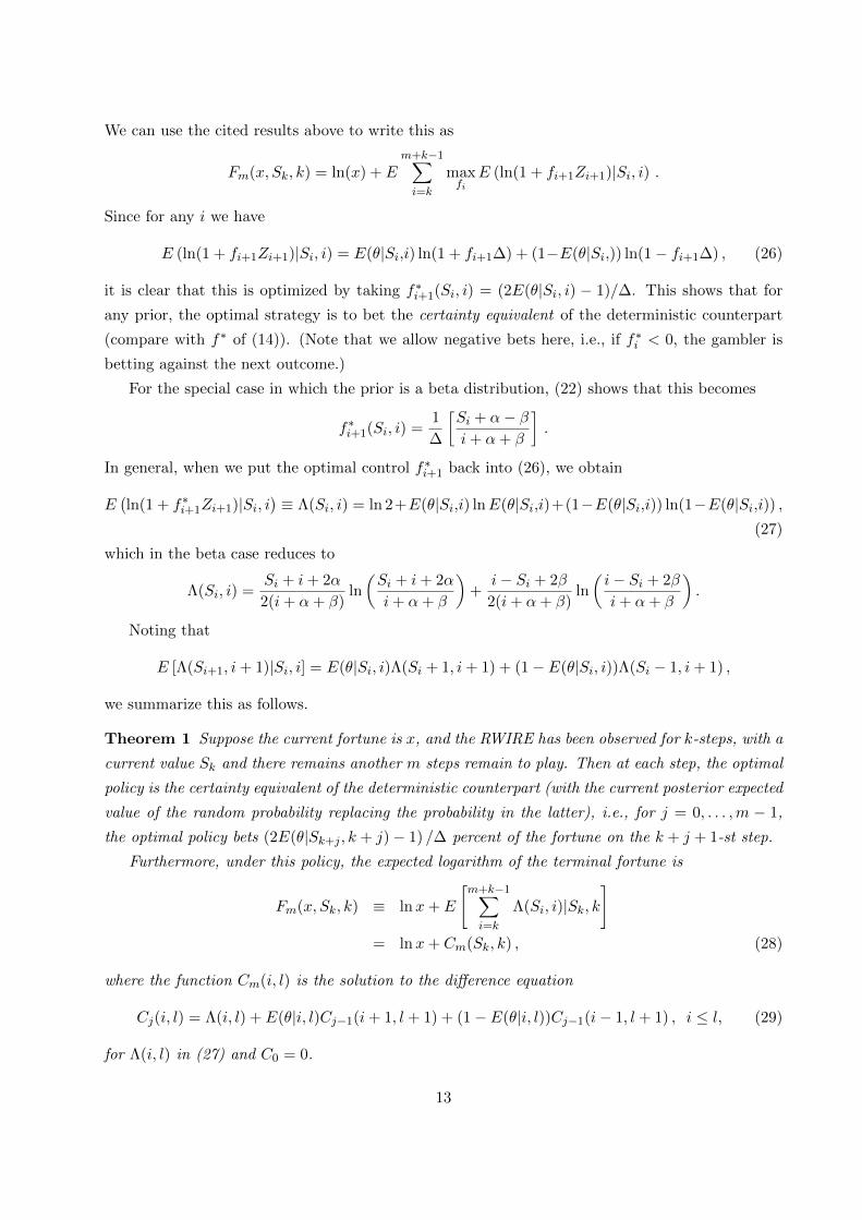
We can use the cited results above to write this as

Fm(x, Sk, k) = ln(x) + Em+k−1∑i=k

maxfi

E (ln(1 + fi+1Zi+1)|Si, i) .

Since for any i we have

E (ln(1 + fi+1Zi+1)|Si, i) = E(θ|Si,i) ln(1 + fi+1∆) + (1−E(θ|Si,)) ln(1− fi+1∆) , (26)

it is clear that this is optimized by taking f∗i+1(Si, i) = (2E(θ|Si, i) − 1)/∆. This shows that for

any prior, the optimal strategy is to bet the certainty equivalent of the deterministic counterpart

(compare with f∗ of (14)). (Note that we allow negative bets here, i.e., if f∗i < 0, the gambler is

betting against the next outcome.)

For the special case in which the prior is a beta distribution, (22) shows that this becomes

f∗i+1(Si, i) =1

∆

[Si + α− βi+ α+ β

].

In general, when we put the optimal control f∗i+1 back into (26), we obtain

E(ln(1 + f∗i+1Zi+1)|Si, i

)≡ Λ(Si, i) = ln 2+E(θ|Si,i) lnE(θ|Si,i)+(1−E(θ|Si,i)) ln(1−E(θ|Si,i)) ,

(27)

which in the beta case reduces to

Λ(Si, i) =Si + i+ 2α

2(i+ α+ β)ln

(Si + i+ 2α

i+ α+ β

)+

i− Si + 2β

2(i+ α+ β)ln

(i− Si + 2β

i+ α+ β

).

Noting that

E [Λ(Si+1, i+ 1)|Si, i] = E(θ|Si, i)Λ(Si + 1, i+ 1) + (1− E(θ|Si, i))Λ(Si − 1, i+ 1) ,

we summarize this as follows.

Theorem 1 Suppose the current fortune is x, and the RWIRE has been observed for k-steps, with a

current value Sk and there remains another m steps remain to play. Then at each step, the optimal

policy is the certainty equivalent of the deterministic counterpart (with the current posterior expected

value of the random probability replacing the probability in the latter), i.e., for j = 0, . . . ,m − 1,

the optimal policy bets (2E(θ|Sk+j , k + j)− 1) /∆ percent of the fortune on the k + j + 1-st step.

Furthermore, under this policy, the expected logarithm of the terminal fortune is

Fm(x, Sk, k) ≡ lnx+ E

[m+k−1∑i=k

Λ(Si, i)|Sk, k]

= lnx+ Cm(Sk, k) , (28)

where the function Cm(i, l) is the solution to the difference equation

Cj(i, l) = Λ(i, l) + E(θ|i, l)Cj−1(i+ 1, l + 1) + (1− E(θ|i, l))Cj−1(i− 1, l + 1) , i ≤ l, (29)

for Λ(i, l) in (27) and C0 = 0.

13

For the beta case, (29) simplifies to

2(l + α+ β)Cj(i, l) + ln(l + α+ β) = (i+ l + 2α) [Cj−1(i+ 1, l + 1) + ln(i+ l + 2α)]

+(l − i+ 2β) [Cj−1(i− 1, l + 1) + ln(l − i+ 2β)] .

It is important to note that the policy obtained above also asymptotically maximizes the asymp-

totic growth rate when used over an infinite-horizon. This follows from Algoet and Cover’s (1988)

infinite-horizon result, for very general discrete processes, that maximizing the conditional expected

log return given all the currently available information at each stage is asymptotically optimal for

maximizing the asymptotic growth rate. In our Markovian model, this reduces to precisely the

policy obtained. However, unlike Algoet and Cover (1988), our main focus is on characterizing

and computing optimal policies explicitly for finite-horizons, which is simplified in the Markovian

setting.

3.4 Adaptive Portfolios

The portfolio problem in discrete time for the RWIRE is also easily solved from the adaptive

gambling results just obtained. Once again the investor has a choice at each step in the RWIRE of

splitting his wager between the next step in the RWIRE and the sure bet (or bond) which has a

fixed return of r per unit time. Analogously to the pure gambling problem, if we allow the random

walk to have step size ∆, in this case we have

Fm(x, Sk, k) = maxfk+1,...,fk+m

E (lnVm+k|Vk = x, Sk, k)

= · · · = ln(x) + Em+k−1∑i=k

maxfi

E (ln(1 + r(1− fi+1) + fi+1Zi+1)|Si, i) .

As before, it is fairly easy to show that the optimal control for the portfolio problem after the

RWIRE has taken i steps is simply to invest the proportion f∗(Si, i) in the random walk, where

(see (13))

f∗(Si, i) =(1 + r) (∆(2E(θ|Si, i)− 1)− r)

∆2 − r2. (30)

Having established that the optimal control for the discrete-time case is simply the certainty

equivalent of the case with a fixed constant probability, we would now like to use this to treat

the continuous-time problem with random parameter values. For such processes, the techniques

of continuous-time stochastic control with partial information become quite complicated (see e.g.

Section VI.10 of Fleming and Rishel (1975)), so rather than studying the continuous-time dynamic

programming optimality equations directly, we would like to employ once again a limiting argument

to the discrete-time process just studied.

To employ this approach, we need a limit theorem that describes precisely how such a random

walk approaches a diffusion. This is the content of the next section.

14

4 Continuous-Time Diffusion Limits

In this section we first establish limits for RWIREs and then we show that the limit, which is a

Brownian motion with a normally distributed random mean, is equivalent to a deterministically

scaled Brownian motion.

4.1 Limits for RWIREs

Recall now, that to send a simple random walk with θ being constant to a simple Brownian motion

with drift, we had to rescale time and space appropriately, and send θ to 1/2 in the appropriate way.

However, if the success probability is a random variable, it is no longer clear how to standardize,

and how to take the limit, and what the resulting limiting process should be. For example, the

central limit theorem for exchangeable random variables shows that for a general density fθ(·), the

normalized random walk converges to a mixed normal distribution, i.e.,

limn→∞

P

(Sn − E(Sn)√

n≤ z

)=

∫ 1

0Φ

(z

2√u(1− u)

)fθ(u) du ,

where Φ denotes the standard normal cdf. No particular simplification occurs here for the case in

which fθ is a beta density. This suggests that to get a reasonable diffusion limit, we need to in fact

take double limits, by allowing the distribution of θ to vary in the appropriate manner with n as

well. We make this precise for the beta case in the following theorem, which we will prove in this

section and make ample use of later.

Theorem 2 Let {Zni } denote a sequence of i.i.d. random variables, with

P (Zni = 1|θn) = θn = 1− P (Zni = −1|θn) ,

where θn ∼ Be(αn, βn) and the parameters αn, βn are given by

αn :=σ2n− (µ2 + c)

2c√n

(√n+

µ

σ

), (31)

βn :=σ2n− (µ2 + c)

2c√n

(√n− µ

σ

). (32)

Let Snm =∑mi=1 Z

ni . Then

σSn[nt]√n⇒ Xt := (σ2 + ct)W t

σ2+ct+ µt , (33)

where Ws is a standard Brownian motion.

Note that under the parameterization above, the prior mean satisfies E(θn) ≡ αnαn+βn

= 1/2 +

µ/2σ√n → 1/2, while the prior variance satisfies V (θn) ≡ αnβn

(αn+βn)2(αn+βn+1)= c/4σ2n → 0.

Furthermore, the unconditional mean and variance of an increment in the n-th random walk satisfies

E(Zni ) = µ/σ√n, and V (Zni ) = 1 − µ2

4σ2n, which are the same as the mean and variance for the

n-th random walk with a constant probability, (see (23) and (24)).

15

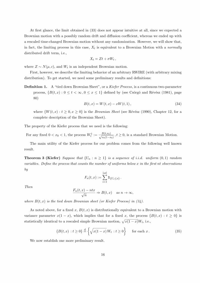
At first glance, the limit obtained in (33) does not appear intuitive at all, since we expected a

Brownian motion with a possibly random drift and diffusion coefficient, whereas we ended up with

a rescaled time-changed Brownian motion without any randomization. However, we will show that,

in fact, the limiting process in this case, Xt is equivalent to a Brownian Motion with a normally

distributed drift term, i.e.,

Xt = Zt+ σWt ,

where Z ∼ N(µ, c), and Wt is an independent Brownian motion.

First, however, we describe the limiting behavior of an arbitrary RWIRE (with arbitrary mixing

distribution). To get started, we need some preliminary results and definitions:

Definition 1. A “tied down Brownian Sheet”, or a Kiefer Process, is a continuous two-parameter

process, {B(t, x) : 0 ≤ t < ∞ , 0 ≤ x ≤ 1} defined by (see Csorgo and Revesz (1981), page

80)

B(t, x) = W (t, x)− xW (t, 1) , (34)

where {W (t, x) : t ≥ 0, x ≥ 0} is the Brownian Sheet (see Revesz (1990), Chapter 12, for a

complete description of the Brownian Sheet).

The property of the Kiefer process that we need is the following:

For any fixed 0 < x0 < 1, the process W 1t := B(t,x0)√

x0(1−x0), t ≥ 0, is a standard Brownian Motion.

The main utility of the Kiefer process for our problem comes from the following well known

result.

Theorem 3 (Kiefer) Suppose that {Un : n ≥ 1} is a sequence of i.i.d. uniform (0, 1) random

variables. Define the process that counts the number of uniforms below x in the first nt observations

by

Fn(t, x) :=

[nt]∑i=1

1{Ui≤x} .

ThenFn(t, x)− ntx√

n⇒ B(t, x) as n→∞,

where B(t, x) is the tied down Brownian sheet (or Kiefer Process) in (34).

As noted above, for a fixed x, B(t, x) is distributionally equivalent to a Brownian motion with

variance parameter x(1 − x), which implies that for a fixed x, the process {B(t, x) : t ≥ 0} is

statistically identical to a rescaled simple Brownian motion,√x(1− x)Wt, i.e.,

{B(t, x) : t ≥ 0} d=

{√x(1− x)Wt : t ≥ 0

}for each x . (35)

We now establish one more preliminary result.

16

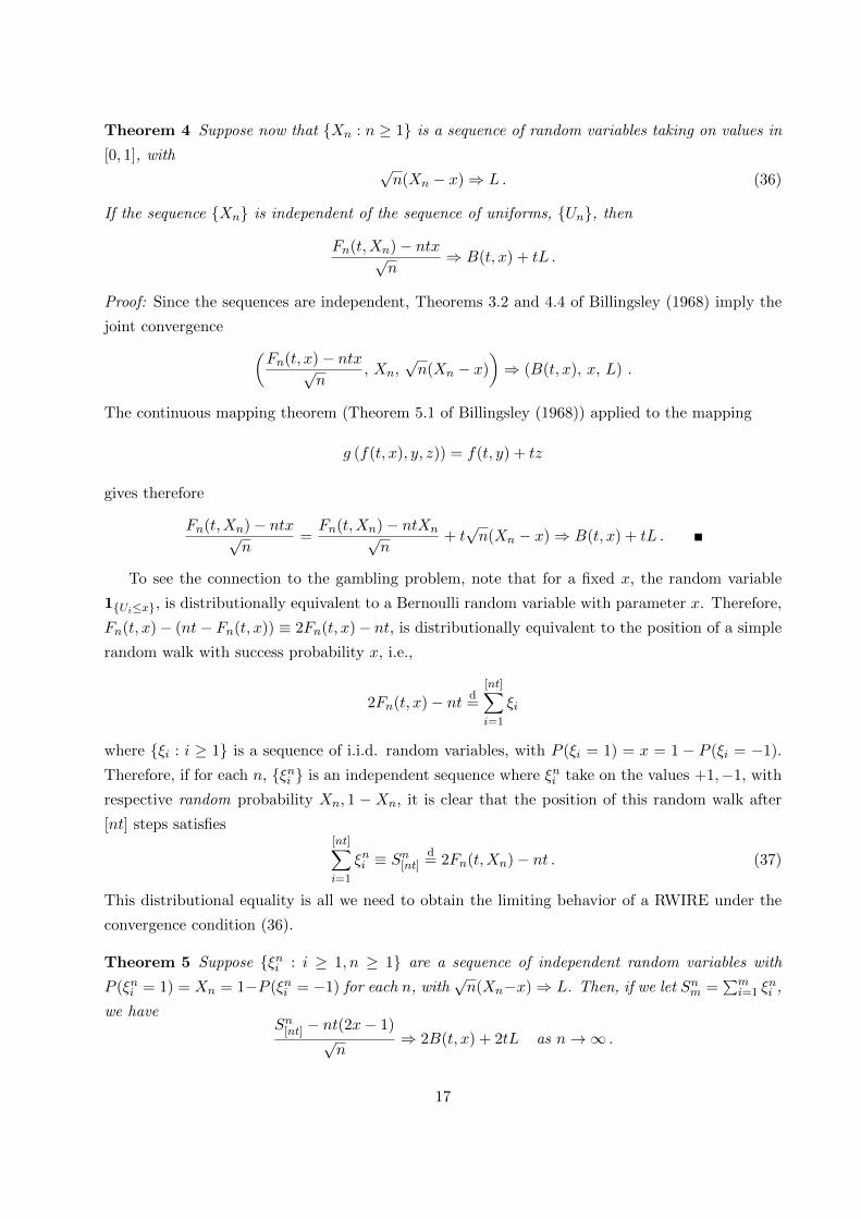
Theorem 4 Suppose now that {Xn : n ≥ 1} is a sequence of random variables taking on values in

[0, 1], with√n(Xn − x)⇒ L . (36)

If the sequence {Xn} is independent of the sequence of uniforms, {Un}, then

Fn(t,Xn)− ntx√n

⇒ B(t, x) + tL .

Proof: Since the sequences are independent, Theorems 3.2 and 4.4 of Billingsley (1968) imply the

joint convergence (Fn(t, x)− ntx√

n, Xn,

√n(Xn − x)

)⇒ (B(t, x), x, L) .

The continuous mapping theorem (Theorem 5.1 of Billingsley (1968)) applied to the mapping

g (f(t, x), y, z)) = f(t, y) + tz

gives therefore

Fn(t,Xn)− ntx√n

=Fn(t,Xn)− ntXn√

n+ t√n(Xn − x)⇒ B(t, x) + tL .

To see the connection to the gambling problem, note that for a fixed x, the random variable

1{Ui≤x}, is distributionally equivalent to a Bernoulli random variable with parameter x. Therefore,

Fn(t, x)− (nt− Fn(t, x)) ≡ 2Fn(t, x)− nt, is distributionally equivalent to the position of a simple

random walk with success probability x, i.e.,

2Fn(t, x)− nt d=

[nt]∑i=1

ξi

where {ξi : i ≥ 1} is a sequence of i.i.d. random variables, with P (ξi = 1) = x = 1 − P (ξi = −1).

Therefore, if for each n, {ξni } is an independent sequence where ξni take on the values +1,−1, with

respective random probability Xn, 1 − Xn, it is clear that the position of this random walk after

[nt] steps satisfies[nt]∑i=1

ξni ≡ Sn[nt]d= 2Fn(t,Xn)− nt . (37)

This distributional equality is all we need to obtain the limiting behavior of a RWIRE under the

convergence condition (36).

Theorem 5 Suppose {ξni : i ≥ 1, n ≥ 1} are a sequence of independent random variables with

P (ξni = 1) = Xn = 1−P (ξni = −1) for each n, with√n(Xn−x)⇒ L. Then, if we let Snm =

∑mi=1 ξ

ni ,

we haveSn[nt] − nt(2x− 1)

√n

⇒ 2B(t, x) + 2tL as n→∞ .

17

Proof: Subtracting nt(2x− 1) from both sides of (37), and dividing by√n, gives

Sn[nt] − nt(2x− 1)√n

d=

2Fn(t,Xn)− 2ntx√n

⇒ 2 [B(t, x) + tL] ,

by the previous Theorem 4.

We now relate the limit in Theorem 5 to standard Brownian motion, Wt, under the condition

that the limiting mean of the random probabilities is 1/2.

Corollary 1 If x = 12 in the setting of Theorem 5, then

Sn[nt]√n⇒Wt + 2tL ,

where Wt denotes a standard Brownian motion.

Proof: Apply the previous Theorem 5, with x = 1/2, to see that in this case we have

Sn[nt]√n⇒ 2B

(t,

1

2

)+ 2tL .

But since B(t, x)d=√x(1− x)Wt, for each x, 0 ≤ x ≤ 1, it is clear that 2B

(t, 12

)d= Wt.

The case in which the success probability has a beta prior, as in Theorem 2, now follows directly.

Corollary 2 In the setting of Theorem 5, if Xn ∼ Be(αn, βn), where αn, βn are given in (31) and

(32), then (36) holds, and thus Corollary 1 holds, with L having a normal distribution, specifically,

L ∼ N(µ2σ ,

c4σ2

).

Proof: First note that under (31) and (32), the mean and variance of Xn satisfy

E(Xn) = αnαn+βn

≡ 1

2+

µ

2σ√n,

V (Xn) = αnβn(αn+βn)2(αn+βn+1)

≡ c

4σ2n,

so that

E

(√n

(Xn −

1

2

))=

µ

2σ, V

(√n

(Xn −

1

2

))=

c

4σ2.

Since the beta distribution converges to the normal when αn = k1 +an+ o(n), βn = k2 + bn+ o(n),

we have√n(Xn − 1

2

)⇒ L, where L ∼ N

(µ2σ ,

c4σ2

).

Since in this case, 2L ∼ N(µσ ,

cσ2

), it now follows directly, that for the random walk displayed

earlier in Theorem 2, with Xn ≡ θn for all n ≥ 1, we have

σSn[nt]√n⇒ σWt + tZ , where Z ∼ N(µ, c).

So the diffusion limit of the mixed, or weighted, random walk described earlier is in fact a Brownian

motion with a random mean. The fact that the distribution of the random drift term, Z, is normally

18

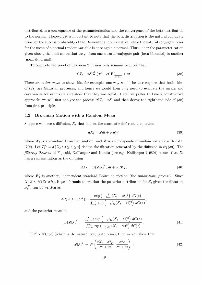
distributed, is a consequence of the parameterization and the convergence of the beta distribution

to the normal. However, it is important to note that the beta distribution is the natural conjugate

prior for the success probability of the Bernoulli random variable, while the natural conjugate prior

for the mean of a normal random variable is once again a normal. Thus under the parameterization

given above, the limit shows that we go from one natural conjugate pair (beta-binomial) to another

(normal-normal).

To complete the proof of Theorem 2, it now only remains to prove that

σWt + tZd= (σ2 + ct)W t

σ2+ct+ µt . (38)

There are a few ways to show this, for example, one way would be to recognize that both sides

of (38) are Gaussian processes, and hence we would then only need to evaluate the means and

covariances for each side and show that they are equal. Here, we prefer to take a constructive

approach: we will first analyze the process σWt + tZ, and then derive the righthand side of (38)

from first principles.

4.2 Brownian Motion with a Random Mean

Suppose we have a diffusion, Xt that follows the stochastic differential equation

dXt = Zdt+ σ dWt (39)

where Wt is a standard Brownian motion, and Z is an independent random variable with c.d.f.

G(z). Let FXt = σ{Xs : 0 ≤ s ≤ t} denote the filtration generated by the diffusion in eq.(39). The

filtering theorem of Fujisaki, Kallianpur and Kunita (see e.g. Kallianpur (1980)), states that Xt

has a representation as the diffusion

dXt = E(Z|FXt ) dt+ σ dWt , (40)

where Wt is another, independent standard Brownian motion (the innovations process). Since

Xt|Z ∼ N(Zt, σ2t), Bayes’ formula shows that the posterior distribution for Z, given the filtration

FXt , can be written as

dP (Z ≤ z|FXt ) =exp

(− 1

2σ2t(Xt − zt)2

)dG(z)∫∞

−∞ exp(− 1

2σ2t(Xt − zt)2

)dG(z)

,

and the posterior mean is

E(Z|FXt ) =

∫∞−∞ z exp

(− 1

2σ2t(Xt − zt)2

)dG(z)∫∞

−∞ exp(− 1

2σ2t(Xt − zt)2

)dG(z)

. (41)

If Z ∼ N(µ, c) (which is the natural conjugate prior), then we can show that

Z|FXt ∼ N

(cXt + σ2µ

σ2 + ct,

σ2c

σ2 + ct

). (42)

19

Therefore, in this case, the filtering theorem implies that Xt is equivalent to the diffusion determined

by the stochastic differential equation

dXt =cXt + σ2µ

σ2 + ctdt+ σ dWt , (43)

where Wt is a standard Brownian motion. This is a linear stochastic differential equation, which

has the strong solution

Xt ≡ µt+ (σ2 + ct)

[X0 +

∫ t

0

σ

σ2 + csdWs

], (44)

(see Karatzas and Shreve, (1988) section 5.6). The mean and covariance functions for this process

are

m(t) := E(Xt) = µt+ (σ2 + ct)E(X0)

ρ(s, t) := E(Xt −m(t))(Xs −m(s)) = (σ2 + cs)(σ2 + ct)

[ρ(0, 0) +

s ∧ tσ2 + c(s ∧ t)

].

We of course have ρ(t, t) := V (t) = (σ2 + ct)[t+ V (0)(σ2 + ct)].

If X0 is constant, and c = 0, then it is clear that Xt is an ordinary Brownian motion with drift

µ and diffusion parameter σ. If not, then if either X0 is constant, or normally distributed, Xt is a

Gaussian process. For notational ease we will, without any loss of generality, always take X0 = 0

for the remainder of the paper.

We now show that the randomized diffusion displayed above has a representation as a sim-

ple time changed Brownian motion, without any randomization. This will complete the proof of

Theorem 2.

Proposition 1 The diffusion process Xt in (44) has the representation

Xtd= (σ2 + ct)W t

σ2+ct+ µt

where {Ws} denotes an independent Brownian motion.

Proof: Suppose we have a diffusion Yt obtained from a standard Brownian motion by the following

transformation:

Yt = a(t)Wg(t) + f(t)

where a(t), g(t), f(t), are all continuous differentiable functions, with g(t) ≥ 0, b(0) = f(0) = 0.

Ito’s formula applied to the above shows that

dYt = [a′(t)Wg(t) + f ′(t)]dt+ a(t)dWg(t).

Since Wg(t) = Yt−f(t)a(t) , and since dWg(t) =

√g′(t) dUt, where Ut is another independent standard

Brownian motion, we can rewrite this last equation as

dYt =a′(t)Yt + a(t)f ′(t)− a′(t)f(t)

a(t)dt+ a(t)

√g′(t) dUt . (45)

20

If we equate the drifts and diffusion parameters of the two stochastic differential equations (45)

and (43), we find

a′(t)Yt + a(t)f ′(t)− a′(t)f(t)

a(t)=

cXt + σ2µ

σ2 + ct, (46)

a(t)√g′(t) = σ . (47)

If we now set Yt = Xt, and then equate the coefficients in (46), we get

a(t) = σ2 + ct , a′(t) = c , (48)

as well as

a(t)f ′(t)− a′(t)f(t) = σ2µ . (49)

When we put (48) into (49), we get the linear ordinary differential equation

f ′(t) =c

σ2 + ctf(t) +

σ2µ

σ2 + ct; f(0) = 0 .

The solution to this is simply f(t) = µt. Eq.(47) now shows that

g′(t) = σ21

a(t)2≡ σ2

(1

σ2 + ct

)2

,

which is easily solved to yield g(t) = tσ2+ct

, and so we’ve established the proposition.

Now, having proved Theorem 2, we can relate the discrete-time Bayesian control problem to

the continuous-time Bayesian control problem.

5 Continuous-Time Bayesian Gambling

We now apply the discrete-time results in section 3 to treat the continuous-time Bayesian gambling

problem, much as we did for the non-Bayesian case in section 2. We first consider gambling and the

financial value of information, then the portfolio problem, and finally we present a final martingale

argument.

5.1 Gambling

Now consider the continuous-time optimal control problem in which your fortune evolves according

to

dVt = ftVt dXt , (50)

where, as before, ft is an admissible control, but now Xt is the Brownian motion with a random

drift term, described above. Thus Vt is not a Markov process, although the two dimensional process

(Vt, Xt) is. Here we will consider the case in which the prior distribution on the drift is a normal with

mean µ, and variance c, which was analyzed previously. What is the optimal policy to maximize

E lnVT ? The answer does not seem evident from the HJB approach, but it seems intuitively clear

that the optimal control should be the certainty equivalent of the deterministic drift case. This

result can be obtained from the discrete-time results in section 3.

21

Theorem 6 The optimal control to maximize the (conditional) expected log of terminal fortune,

for any terminal time is to invest at time t the fraction

f∗t =1

σ2

(cXt + µσ2

σ2 + ct

)(51)

which is simply the posterior mean drift of the underlying diffusion, Xt, divided by its diffusion

coefficient, i.e., the certainty equivalent of (8).

Proof: By (42) and (43), we see that (51) is the certainty equivalent of (8). The optimality of

(51) follows from the same type of limiting argument as we used for the simple random walk with

constant success probability. We will first show that f∗t is the appropriate limit of the controls

of the discrete-time optimal control. We will then verify that f∗t is in fact the optimal control

by a martingale argument. To proceed, the development in section 3 shows that if we consider a

sequence of RWIREs, the n-th of which has success probability θn, and step size σ/√n, then the

optimal policy is to bet

f∗(Snk , k) =2E(θn|Snk )− 1

σ/√n

at the k-th step. To show that the limit of the controls for the random walks converge to the

optimal control for the corresponding diffusion, i.e., that f∗(Sn[nt], [nt])⇒ f∗t , where f∗t is given by

(51), we need the following corollary to Theorem 2, which gives the weak convergence result for

the drift of the sequence of RWIREs.

Corollary 3 Under the conditions of Theorem 2,

2E(θn|Sn[nt])− 1

σ/√n

⇒ 1

σ2

(cXt + µσ2

σ2 + ct

). (52)

Proof: By (22),

2E(θn|Snk )− 1 =Snk + αn − βnk + αn + βn

. (53)

By (53), (31), (32) and Theorem 2

2E(θn|Sn[nt])− 1

σ/√n

=

Sn[nt]√n

+ µσc −

µcσ

(µ2+cn

)σ(t+ σ2

c −(µ2+c)cn

) ⇒ 1

σ2

(cXt + µσ2

σ2 + ct

).

Of course, we have not yet proved that f∗t given by (51) is in fact the optimal policy for the

continuous time problem, but only that it is the weak limit of the discrete-time optimal controls.

We will in fact verify this (in greater generality) after we discuss the portfolio problem. We note

now however, that under the policy given above, the optimal fortune evolves as

dV ∗t = V ∗t

1

σ2

(cXt + µσ2

σ2 + ct

)2

dt+1

σ

(cXt + µσ2

σ2 + ct

)dWt

, V ∗0 = x , (54)

22

which can be verified by placing (51) and (43) into (50). This allows us to compare the Bayesian

gambler with the constant gambler and the gambler with perfect information as in Section 2.3.

Barron and Cover (1988) have developed general bounds on the growth rate of wealth for various

stages of information in terms of conditional entropy measures. Due to the specific parametric form

of the model considered here, (54) will enable us to characterize these quantities to a very explicit

degree.

5.2 The Financial Value of Randomness and Information

Under the optimal Bayesian policy, the gambler’s fortune evolves as (54), and therefore by Ito’s

formula we find

lnV ∗T = lnx+1

2σ2

∫ T

0

(cXt + µσ2

σ2 + ct

)2

dt+1

σ

∫ T

0

(cXt + µσ2

σ2 + ct

)dWt , (55)

which is the continuous-time limit of (28). If we let FBT (x) denote the optimal value function for

the Bayesian gambler, then taking expectations on (55) using (44) shows

FBT (x) := E lnV ∗T = lnx+µ2

2σ2T +

c

2σ2T +

1

2ln

(σ2

σ2 + cT

). (56)

Comparing this with (10) and (12) shows that for any T > 0, the optimal value in the Bayesian

case is always sandwiched between the optimal value of the constant gambler and the gambler who

randomizes with perfect information, i.e.,

FT (x) ≤ FBT (x) ≤ FPT (x).

Thus while the randomness in the model is helping the Bayesian gambler do better than the constant

gambler, he of course cannot do better than the gambler with perfect information. However, it

appears that in fact, he does substantially better than the constant gambler since

FBT (x)− FT (x) =c

2σ2T +

1

2ln

(σ2

σ2 + cT

), (57)

which is convex increasing in the horizon T , while only slightly less than the gambler with perfect

information. In particular, we see from (12) and (56) that the financial cost of learning is logarithmic

since

FPT (x)− FBT (x) =1

2ln

(1 +

c

σ2T

). (58)

This should be considered the financial value of perfect information, since it is how much the

Bayesian gambler should be willing to pay to learn the true value of Z.

We note that FT (x) given by (10) is also the value under the Bayesian model for a gambler

who always invests according to the prior expected value, i.e., a gambler who always invests the

constant fraction µ/σ2, and whose fortune therefore evolves as dVt = (µ/σ2)Vt dXt, for dXt in (43).

23

Therefore (57) can be considered the financial gain of using the posterior over the prior. From (57)

we find that the expected marginal benefit of increasing the horizon T to the gambler using the

posterior over the prior is

∂

∂T

(FBT (x)− FT (x)

)=

c2

2σ2

(T

σ2 + cT

)→ c

2σ2, as T →∞

while from (58) we find that the expected marginal benefit of increasing the horizon to the gambler

with perfect information over the Bayesian gambler is

∂

∂T

(FPT (x)− FBT (x)

)=

c

2σ2

(1

σ2 + cT

)→ 0 , as T →∞ .

5.3 Adaptive Portfolios

Similarly, if we consider the portfolio problem associated with a sequence of RWIREs, where the

nth random success probability is θn, and the step size is δn, it follows that the optimal control is

to invest, at time [nt] in the nth random walk, the fraction (see (30))

f∗(n)(Sn[nt], [nt]) =(1 + r)

(δn(2E(θn|Sn[nt])− 1)− r

)δ2n − r2

. (59)

The optimal control for the resulting diffusion control problem, i.e., for the portfolio problem

where the drift of the Brownian motion has a normal distribution, can now be obtained with the

aid of the previous results.

Suppose an investor is faced with the diffusion control problem of maximizing E(lnVT ), where

the return process of the risky stock, Xt, is a Brownian motion with a random, normally distributed

drift. I.e., in the context of Merton’s (1971) model, we will assume that the price of the risky stock,

St, and the price of the riskless bond, Bt, evolve respectively as

dSt = ZStdt+ σStdWt and dBt = γBtdt

where Wt is a standard Brownian motion, and Z is an independent unobserved random variable

with a normal distribution, as before. If we define the return process, Xt, associated with the stock

price process St by

Xt :=

∫ t

0

1

SudSu (60)

then it follows from our previous results that in this case, the extension of Merton’s control problem

is equivalent to solving for the optimal admissible control process {ft : 0 ≤ t ≤ T}, to maximize

E lnVT , where now

dVt = Vt(1− ft)γ dt+ Vtft dXt (61)

dXt =cXt + σ2µ

σ2 + ctdt+ σ dWt. (62)

24

(Note that a simple application of Ito’s rule shows that Xt = lnSt + tσ2/2, where S0 = 1, since

we’ve assumed that X0 = 0.)

In this case, the problem is clearly more complicated than in the nonrandom case. However,

an appeal to our previous results will again give us the optimal control without resorting to the

HJB techniques. The optimal control is the certainty equivalent of the optimal control (16) first

obtained by Merton (1971) for the nonrandom case.

Theorem 7 In the context of (61) and (62) the optimal control is

f∗t =1

σ2

(cXt + µσ2

σ2 + ct− γ

). (63)

Proof: We will show that f∗(n)(Sn[nt], [nt]) ⇒ f∗t . To see that this is true, substitute for the step

size, δn = σ/√n, as well as for the interest rate, in terms of the interest rate per step, i.e., r = γ/n,

in (59), to rewrite it as

f∗(n)(Sn[nt], [nt]) =

(1 +

γ

n

) σn

(2E(θn|Sn[nt])− 1

)− γ

n

σ2

n −γ2

n2

=

(1 + γ

n

)(1− γ2

σ2n

) (2E(θn|Sn[nt])− 1

σ/√n

− γ

σ2

)

⇒ 1

σ2

(cXt + µσ2

σ2 + ct

)− γ

σ2

by (52).

5.4 The Final Martingale Argument

It remains now to verify that the limiting controls obtained above are in fact the optimal ones

for the continuous-time problems. In fact, more is true. We have concentrated on the natural

conjugate case (where Z was assumed to have a normal distribution) only for the sake of analytical

tractability. However, as we now show, the optimality of the certainty equivalent holds for arbitrary

prior distributions, i.e., regardless of the parametric form of the distribution of the unobserved

random variable, Z, the optimal control is to invest

f∗t =1

σ2

[E(Z|FXt )− γ

](64)

in the risky stock, where {FXt : t ≥ 0} denotes the filtration of the return process X defined in (60).

Note that (64) is the general certainty equivalent of (16), and that E(Z|FXt ) can be computed for

arbitrary prior distributions from (41).

To verify the optimality of the policy f∗t of (64), apply Ito’s rule to the semi-martingale lnVt,

where Vt is given by (61) but where dXt is given by the more general (40) to get

d lnVt =1

VtdVt −

1

2V 2t

d < V >t

25

where< V >t is the quadratic variation of the semi-martingale Vt, and note that< V >t= f2t V2t σ

2 t.

Therefore, we have

d lnVt = (1− ft)γ dt+ ftdXt −1

2f2t σ

2 dt

=

[(1− ft)γ + ftE(Z|FXt )− 1

2f2t σ

2]dt+ ftσ dWt ,

where the last equality follows from (40). Integrating from 0 to T , and then taking conditional

expectations – recognizing that the posterior mean of Z, E(Z|FXt ), is a function of just Xt alone

(see (41)) – shows that

E(lnVT | FXT−

)=

∫ T

0

[(1− ft)γ + ftE(Z|FXt )− 1

2f2t σ

2]dt . (65)

Since the right-hand-side of (65) does not contain the process Vt, it is clear that it suffices to

maximize the integrand pointwise with respect to ft, which will result in the optimal control f∗t

given above in (64). For the special case where the prior is normal, this of course reduces to the

policy of (63). Thus we may conclude that the policies given above are in fact optimal for the

continuous-time problems.

6 Other Utility Functions

For the objective of maximizing log utility, we have shown that the optimal policy for the RWIRE

as well as for the Brownian motion with a random mean, is the certainty equivalent of respectively

the ordinary random walk and the ordinary Brownian motion, i.e., the optimal control for the case

of a random parameter is obtained by just substituting the current conditional expected value of

the random parameter (µ) in place of the known parameter in the control policy for the case of the

known parameter.

This raises the question of whether a similar result holds for other objective functions as well.

While we do not have the full answer to this question, we do observe that this is not true for the case

of a power utility function. In fact, Bellman and Kalaba (1957) proved that a purely proportional

betting scheme is optimal only for the case where the gambler is interested in maximizing E(V ηT /η+

κ) for 0 ≤ η ≤ 1, and for some constant κ. (The logarithmic case occurs in the limit as η → 0

when κ = −1/η.) A somewhat more general result for continuous-time problems was found by

Merton (1971), for what he referred to as the HARA (hyperbolic-absolute-risk-aversion) class of

utility functions.

Now, since for η > 0 the strategy that maximizes E(V ηT /η+ κ) is the same as the strategy that

maximizes E(V ηT ), without any loss in generality, we will suppose that the investor’s objective is to

maximize E(V ηT ), for 0 < η < 1. For notational ease, we will consider only the case of r = γ = 0.

We can no longer use the simple approach of Sections 2 and 3 to determine the optimal utility as

well as the optimal policy. For this case, we must use the technique of dynamic programming. If

26

we let Fm(x) denote the optimal value function with m bets to go and with a current fortune of x,

then when all parameters are known constants, the optimality equation for this problem is

Fm(x) = maxf{θFm−1(x+ fx∆) + (1− θ)Fm−1(x− fx∆)} ,

with the boundary condition F0(x) = xη. For m = 1, we have

F1(x) = maxf{θ(x+ fx∆)η + (1− θ)(x− fx∆)η}

= xη maxf{θ(1 + f∆)η + (1− θ)(1− f∆)η}

from which a simple computation yields the optimizer

f∗ =1

∆

θ 11−η − (1− θ)

11−η

θ1

1−η + (1− θ)1

1−η

, (66)

and associated optimal value

F1(x) = xη [C(θ, η)]

for

C(θ, η) = 2η(θ

11−η + (1− θ)

11−η)1−η

. (67)

Induction then shows that for a horizon of length N , the optimal policy is in fact to invest the

same fixed fraction f∗ of (66) at each stage, with a final terminal value

FN (x) = xη [C(θ, η)]N .

The optimal policy for the continuous time case can be obtained from this by letting f∗n denote

the optimal control for the nth random walk, with θn = 12

(1 + µ

σ√n

), and ∆ = δn = σ/

√n in (66).

Letting ε = 11−η , and then expanding around 0, we see that

f∗n =1

δn

(θεn − (1− θn)ε

θεn + (1− θn)ε

)

=

√n

σ

2ε( µσ√n

) + o(n−2)

2 + o(n−2)

→ εµ

σ2≡ µ

σ2(1− η),

which is in fact the optimal control for the continuous-time problem (see Merton (1971) or Karatzas

(1989)).

Since the optimal control for the case of a power utility function is again a fixed fraction,

it is natural to expect that the Bayesian controls might then be the certainty equivalent of these

constants. However, the Bayesian case breaks down already for a two-step horizon. In the Bayesian

discrete-time problem, the dynamic programming equation is given by

Fm(x, Sk, k) =

maxf{E(θ|Sk,k)Fm−1(x+fx, Sk+1, k+1) + (1−E(θ|Sk,k))Fm−1(x−fx, Sk−1, k+1)} ,

27

with the terminal boundary condition F0(x, Sk, k) = xη. Thus for a one-step horizon, the Bellman

equation is

F1(x, Sk, k) = maxf{E(θ|Sk, k) (x+ fx∆)η + (1− E(θ|Sk, k)) (x− fx∆)η} (68)

and the optimizer is

f∗(Sk, k) =1

∆

[E(θ|Sk, k)]1

1−η − [1− E(θ|Sk, k)]1

1−η

[E(θ|Sk, k)]1

1−η + [1− E(θ|Sk, k)]1

1−η

, (69)

which is the certainty equivalent of the nonrandom case. When the optimal control is placed back

into the Bellman equation (68), we get the optimal value function

F1(x, Sk, k) = xη · C (E(θ|Sk, k), η)

where the function C is given by (67). Since F1(x, Sk, k) = F0(x, Sk, k)C, it is clear that for a

two-step horizon the optimality equation can be written as

F2(x, Sk, k) = xη maxf{E(θ|Sk, k) · (1 + f)ηC (E(θ|Sk + 1, k + 1), η)

+ (1− E(θ|Sk, k)) · (1− f)ηC (E(θ|Sk − 1, k + 1), η)} ,

resulting in the optimizer

f∗2 (x, Sk, k) =

(1

∆

)[θk(Sk)θk+1(Sk+1)]ε

+[θk(Sk)θk+1(Sk+1)

]ε−[θk+1(Sk−1)θk(Sk)

]ε−[θk+1(Sk−1)θk(Sk)

]ε[θk(Sk)θk+1(Sk+1)

]ε+[θk(Sk)θk+1(Sk+1)

]ε+[θk+1(Sk−1)θk(Sk)

]ε+[θk+1(Sk−1)θk(Sk)

]εwhere ε := 1/(1− η), θj(y) := E(θ|Sj = y, j), and z := 1− z.

Clearly, the optimal control in this case is not the certainty equivalent, and thus it appears that

the continuous-time optimal control will also not be the certainty equivalent.

We may in fact continue the iteration to show that the Bayesian optimal control, after observing

the random walk for k steps, with j steps left to go, is to invest the fraction

f∗j (x, Sk, k) =

(1

∆

) [θk(Sk)gj−1(k + 1, Sk + 1)]ε−[θk(Sk)gj−1(k + 1, Sk − 1)

]ε[θk(Sk)gj−1(k + 1, Sk + 1)

]ε+[θk(Sk)gj−1(k + 1, Sk − 1)

]ε (70)

where the functions gl(r, v) are defined by the nonlinear difference equations

gl(r, v) =

([θr(v)g

l−1(r + 1, v + 1)

]ε+[θr(v)g

l−1(r + 1, v − 1)

]ε)1/ε

(71)

with g0 = 1.

A similar analysis can be given for other utility function such as the exponential, where the

investor is interested in maximizing E (a− b exp{−λVT }). In this case too the discrete-time optimal

28

control in the Bayesian case is also not the certainty equivalent. However, since an exponential

utility function does not lead to a proportional strategy for the case in which the parameters are

known constants, we will not pursue this here.

It would appear from the development in Section 3 that a sufficient condition for the Bayesian

control to be the certainty equivalent of the deterministic control is that the optimal value function

be completely separable, i.e., that

Fj(x, Sk, k) = Fj−1(x, Sk, k) + ψ(Sk, k)

where ψ(·) is independent of the wealth x. This is the case for the logarithmic utility, but not for

power utilities nor exponential.

The question of what the optimal controls of (70) converge to remains to be determined.

7 Concluding Remarks

Besides the problems just outlined for utility functions other than the logarithmic, four important

issues still remain open: First, we need to prove for both the Bayesian and non-Bayesian problems

that the discrete-time results directly imply optimality for the limiting controls. Second, we need to

establish limits in the Bayesian setting for more general gambles than simple random walks. Third,

we need to determine useful conditions on general priors (and even priors for simple random walks

(beyond (36)) for the posterior means to be well behaved, i.e., to be in the domain of attraction of a

normally distributed random drift of a Brownian motion. Finally, it would be nice to consider more

general models in which the success probability of the simple random walk is itself an unobserved

stochastic process instead of just a fixed random variable.

References

[1] Algoet, P.H. and Cover, T.M. (1988) Asymptotic Optimality and Asymptotic Equipartition

Properties of Log-Optimum Investment. Ann. of Probab., 16, 876-898.

[2] Barron, A. and Cover, T.M. (1988) A Bound on the Financial Value of Information. IEEE

Trans. Info. Theory, 34, 1097-1100.

[3] Bell, R.M., and Cover, T.M. (1980) Competitive Optimality of Logarithmic Investment. Math.

Oper. Res., 5, 161-166.

[4] Bellman, R. and Kalaba, R. (1957) On the Role of Dynamic Programming in Statistical

Communication Theory. IRE (now IEEE) Trans. Info. Theory, Vol. IT, 3, 197-203.

[5] Billingsley, P. (1968) Convergence of Probability Measures, Wiley.

[6] Breiman, L. (1961) Optimal Gambling Systems for Favorable Games. Fourth Berkeley Symp.

Math. Stat. and Prob., 1, 65 - 78.

29

[7] Cover, T.M. (1991). Universal Portfolios, Mathematical Finance, 1, 1-29.

[8] Cover, T.M. and Gluss, D.H. (1986). Empirical Bayes Stock Market Portfolios, Adv. Appl.

Math., 7, 170-181.

[9] Cover, T.M. and Thomas, J. (1991) Elements of Information Theory, Wiley.

[10] Csorgo, M. and Revesz, P. (1981) Strong Approximations in Probability and Statistics, Aca-

demic Press.

[11] DeGroot, M.H. (1970) Optimal Statistical Decisions, McGraw-Hill.

[12] Ethier, S.N. (1988). The proportional bettor’s fortune. Proc. 5th International Conference on

Gambling and Risk Taking, 4, 375-383.

[13] Ethier, S.N. and Tavare, S. (1983) The proportional bettor’s return on investment. J. Appl.

Prob., 20, 563 - 573.

[14] Feller, W. (1971) An Introduction to Probability Theory and its Applications, Vol.2, 2nd ed.,

Wiley.

[15] Finkelstein, M. and Whitely, R. (1981) Optimal Strategies for repeated games. Adv. Appl.

Prob., 13, 415 - 428.

[16] Gottlieb, G. (1985) An optimal betting strategy for repeated games. J. Appl. Prob., 22, 787 -

795.

[17] Hakansson, N. (1970) Optimal investment and consumption strategies under risk for a class of

utility functions. Econometrica, 38, 587 - 607.

[18] Heath, D., Orey,S., Pestien, V. and Sudderth, W. (1987) Minimizing or Maximizing the ex-

pected time to reach zero. SIAM J. Cont. and Opt., 25, 195-205.

[19] Jamishidian, F. (1992). Asymptotically Optimal Portfolios, Mathematical Finance, 2, 131-150.

[20] Kallianpur, G. (1980) Stochastic Filtering Theory, Springer-Verlag.

[21] Karatzas, I. (1989) Optimization Problems in the Theory of Continuous Trading. SIAM J.

Cont. and Opt., 7, 1221-1259.

[22] Karatzas, I. and Shreve, S. (1988) Brownian Motion and Stochastic Calculus, Springer-Verlag.

[23] Kelly, J. (1956) A New Interpretation of Information Rate. Bell Sys. Tech. J., 35, 917 - 926.

[24] Kurtz, T.G. and Protter, P. (1991) Weak Limit Theorems for Stochastic Integrals and Stochas-

tic Differential Equations. Ann. Probab., 19, 1035-1070.

[25] Kushner, H.J. and Dupuis, P.G. (1992) Numerical Methods for Stochastic Control Problems in

Continuous-Time, Springer-Verlag.

30

[26] Latane, H. (1959) Criteria for choice among risky assets. J. Polit. Econ., 35, 144 - 155.

[27] Merton, R. (1971) Optimum Consumption and Portfolio Rules in a Continuous Time Model.

J. Econ. Theory, 3, 373-413.

[28] Merton, R. (1990) Continuous Time Finance, Blackwell.

[29] Pestien, V.C., and Sudderth, W.D. (1985) Continuous-Time Red and Black: How to control

a diffusion to a goal. Math. Oper. Res., 10, 599-611.

[30] Revesz, P. (1990) Random Walk in Random and Non-Random Environments, World Scientific.

[31] Thorp, E.O. (1969) Optimal gambling systems for favorable games. Rev. Int. Stat. Inst., 37,

273 - 293.

[32] Thorp, E.O. (1971). Portfolio Choice and the Kelly Criterion, Bus. and Econ. Stat. Sec.,

Proc. Amer. Stat. Assoc., 215-224.

31