Populations and our place in the Biosphere

To begin understanding populations, remember thedefinition of ecology:

Ecology is the study of the distribution and abundance of species (or populations).It is also the study of causes of those distributions and abundances.

What kinds of distributions are typically seen innatural populations?

Three kinds represent pigeonholes along what isreally a continuous distribution of kinds:

1) random

2) regular (or overdispersed)

3) clumped (or contagious)

1) Randomly - one example is the distribution oftrees of a single species in the diverse andcomplex tropical forest.

2) Regular - (or uniform or overdispersed) -One example of this distribution include the penguins shown below on nesting territories.Each one is just beyond the reach of its neighbors. Another is the spacing of creosotebushes, each poisoning the ground around it.

3) clumped - organisms ‘gather’ where conditionsare better for them. When you measurepopulation density, it is higher where conditionsare better. This is, especially when viewed froma larger perspective, the most common pattern.

With that background about distribution, what aboutabundance?

Populations are dynamic. They grow in size (number).

Growth seems to follow two different patterns:

1) Exponential (or density-independent) growth2) Logistic (or density-dependent) growth

If a real population grew indefinitely, it wouldeventually follow the logistic pattern (because the resources supporting it are not infinite, but somespecies (like insects) grow seasonally, and duringtheir growing season, grow essentially exponentially.

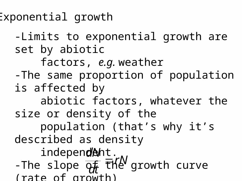
Exponential growth

-Limits to exponential growth are set by abiotic factors, e.g. weather-The same proportion of population is affected by abiotic factors, whatever the size or density of the population (that’s why it’s described as density independent.-The slope of the growth curve (rate of growth) increases as population grows, and in direct proportion to the size. Mathematically:dN

dtrN

Graphically:

The 1.0 and 0.5 are values of r, the growth rate perunit of time. N is the population size.

Populations that seem to grow exponentially stillhave a carrying capacity - a population size thatcan be supported by prevailing conditions andresources.

Some populations growing exponentially can,due to their rapid rates of increase, temporarilyexceed the carrying capacity. Those populationsthen crash to sizes well below carrying capacity.Think of this as boom and bust.

time

#carrying capacity, K

Logistic growth

-Limits to growth are set by biotic factors, e.g. food, interactions with other species like competition or predation-The growth curve at low density looks like the exponential, but slope and growth rate decline as numbers increase, until there is no further growth when population size reaches K, the carrying capacity.-The proportion affected increases with density (so this growth pattern is called density-dependent.

Mathematically:

Graphically:

The data points are a real growth curve for Paramecium ina culture flask.

dN

dtrN

K N

K

Biological interactions influence growth rate:

a) predation, parasitism (and disease, which isa form of parasitism) reduce growth rate

b) predators and parasites are more likely toencounter and attack members of a populationas its density increases

c) competition, both between species and amongmembers of this population, has greater impact as density increases

d) stresses in the denser population also increasethe likelihood that members will emigrate

e. Thus, the growth rate slows as the carrying capacity is approached. In theory, growth ceases, and the population reaches an equilibrium at the carrying capacity.f. Due to the shape of the growth curve (basically S-shaped), logistic growth is sometimes described as ‘sigmoid’.

What processes determine the changes in populationsize?

Birth - adds new individuals to a populationDeath - removes the dying from the populationImmigration - brings new individuals into itEmigration - individuals leave, decreasing the

population

We usually disregard immigration and emigrationin simple models of population growth.

Instead we study the demography of the population.

Demography is the study of the age-specificsurvivorship and reproduction of individuals in apopulation. From these we can predict whether apopulation is going to grow, remain stable, or decline.

There are two approaches: numerical and quantitativeor descriptive and graphical.

First the graphical approach:a “demographers curve” plots the fractions of apopulation in each age class, separating males and females

Note the differences in shapes of demographers’curves for Sweden, Mexico, and the U.S.What do the differences tell us?

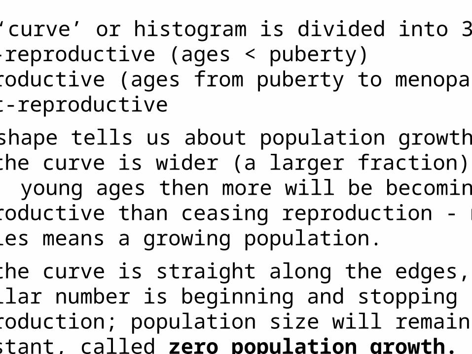
1. The ‘curve’ or histogram is divided into 3 regions:pre-reproductive (ages < puberty)reproductive (ages from puberty to menopause)post-reproductive

2. The shape tells us about population growth:If the curve is wider (a larger fraction) in the

young ages then more will be becoming reproductive than ceasing reproduction - more babies means a growing population.

If the curve is straight along the edges, asimilar number is beginning and stoppingreproduction; population size will remain constant, called zero population growth.

3. When there’s a ‘hump’ in the curve (go back and look at the curve for the U.S.), it indicates a transient increase in the number of babies - a “baby boom”. These data clearly show the post- WWII boomers.

Now the quantitative approach: structure and use of alife table.

In a life table we follow a cohort (a group of organismsborn at the same time), recording how many are aliveat each time interval, and how many young each femalehas during the interval.

The numbers in the life table are:a) age structure - the age classesb) survivorship - how many from the cohort

(what fraction?) are still alive at age x?c) age specific natality - how many young are

born to females of each age?

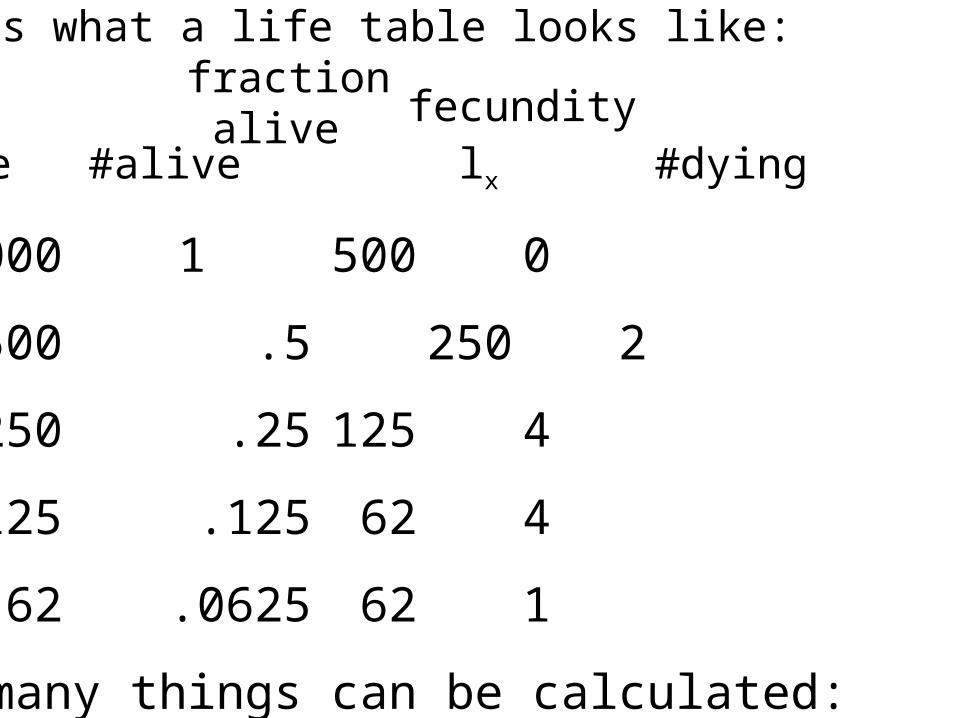
Here’s what a life table looks like: fraction alive fecundity

Age #alive lx #dying mx

0 1000 1 500 0

1 500 .5 250 2

2 250 .25 125 4

3 125 .125 62 4

4 62 .0625 62 1

From it many things can be calculated:

1) population growth rate (r) - combines survivorship and natality (births) into an instantaneous growth rate. It is analogous to the interest rate on your bank account (if the bank compounded instantaneously). However, no bank compounds instantaneously; the best available is daily compounding.

2) how much longer is an organism already x years old likely to live? This is what your insurance needs to know. It is called ex (or life expectancy).

There are typical patterns for a curve of survivorshipover the lifespans of organisms. There are 3 patternsrepresenting a continuum of possibilities:

Type I - organisms live out a very large fraction oftheir genetically programmed maximumlifespan. Humans and other large mammalshave this survivorship pattern.

Type II - organisms suffer a constant proportionalmortality over time, e.g. the sample life table.Perching birds and bats are good examples ofthis survivorship.

Type III - suffer very high mortality in initial periodsof life, but have high survivorship thereafter.A maple tree, oyster, or salmon are good

examples here.

There are also characteristic patterns of natality, and they are associated with the survivorships. In sum, patterns in survivorship and natality are called:Life History Patterns

Again there is a continuum, but we recognize differences between the extremes:

opportunistic (r-selected, weedy) species - typically capable of rapid growth when conditions are good

versusequilibrial (K-selected, climax) species - grow only slowly, but maintain populations near carrying capacity, K.

Characteristics Opportunistic Equilibrial

Age of 1st early, low later, older reproductionlitter size large smallsize of offspring small largeparental care no variable,

some yesorganism size typically small typically largepopulation size variable - small stable - highgrowth pattern frequently looks logistic

exponential