population forecast errors: a primer for planners

Population Forecast Errors: A Primer for Planners

Stefan Rayer, University of Florida

Final formatted version published in Journal of Planning Education and Research, February

2008, Volume 27, pp 417–430. DOI: 10.1177/0739456X07313925

Abstract

Projections of future populations are integral to many planning applications, yet are often poorly

understood. This analysis focuses on the implications of the choices planners make when they

construct projections. Specifically, it examines the impact of length of base period, analyzes the

error structure of projection techniques for counties in the aggregate and by size and growth

rates, investigates the role of averaging, and compares the performance of trend extrapolation

and cohort–component methods. The article concludes by discussing forecast complexity, data

quality, the role of assumptions, and other considerations of forecasting in a planning context.

Keywords: Population projections; model specification; forecast accuracy; averaging

techniques; trend extrapolation; complexity.

1

Introduction

Calculations of future populations are used extensively in urban and land use planning; for

economic development initiatives; for infrastructure, transportation, and health services

planning; for water demand assessments; for natural resource management and protection;

among other applications. According to Myers (2001, 384), “planning analysts regard population

statistics as integral to virtually all aspects of planning,” yet he laments that the demographic

approach has been underutilized by the discipline. This is unfortunate, because planners are in a

unique position to shape the future (Isserman 1985; Myers and Kitsuse 2000).

Predicting future population change involves the application of demographic methods by

which a population is projected or forecasted. Demographic convention considers projections to

be conditional statements about the future, which reflect the outcome of particular assumptions,

and which are always correct unless there was an error in their calculation, while forecasts are

unconditional statements that reflect what the analyst believes most likely to happen in the future

(Isserman 1984; Shryock and Siegel 1976). The terms projection and forecast are used

interchangeably in this article because, as Keyfitz (1972, 353) noted, “a demographer makes a

projection, and his reader uses it as a forecast.”

Planners and other practitioners that produce population forecasts are faced with making

decisions regarding the choice of methods, input data, assumptions, treatment of special

populations, etcetera. The evaluation criteria discussed in this paper are targeted at both

producers and users to provide a better understanding of what matters for small area projections

of total population. In particular, the study pursues three primary objectives. The first is to

investigate the relationship between the length of the projection horizon and the base period with

regard to forecast accuracy. The second is to analyze forecast errors for commonly-used horizon

2

lengths, first for all counties, and then by population size and growth categories. The third is to

examine forecast error by forecast technique, comparing individual trend models to various

averages, and cohort-component models to trend extrapolation techniques. The paper concludes

with a discussion of the evaluation criteria analyzed in this study, as well as data quality and

related issues that also affect forecast outcomes.

Criteria for Evaluating Population Projections

Population projections can be evaluated on many grounds. Smith, Tayman, and Swanson (2001),

in their review of the literature, list in this regard provision of necessary detail, face validity,

plausibility, costs of production, timeliness, ease of application and explanation, usefulness as an

analytical tool, political acceptability, and forecast accuracy. Depending on the situation,

producers and users place different emphases on the importance of these criteria, but for many

forecast accuracy is paramount (Mentzer and Kahn 1995; Yokum and Armstrong 1995). Because

planning decisions and funding allocations are often tied to calculations of future populations, it

is critical to pay attention to forecast accuracy.

For planners, though, accuracy is not everything (Sawicki 1989). Forecasting in planning

practice often contains an inherent conflict between pure or analytic forecasts on the one hand,

and normative or advocacy forecasts on the other hand (Isserman 2007; Wachs 1989). Accuracy

is of less interest for advocacy forecasts, for “if some political purpose was being served by

making a forecast, that forecast need not really be correct in order for it to have its intended

effect” (Wachs 2001, 369). Taken to the extreme, “planners on the dark side are busy not with

getting forecasts right and following the AICP Code of Ethics but with getting projects funded

and built. And accurate forecasts are often not an effective means for achieving this objective.

3

Indeed, accurate forecasts may be counterproductive, whereas biased forecasts may be effective

in competing for funds and securing the go-ahead for construction” (Flyvbjerg, Skamris Holm,

and Buhl 2005, 142).

This analysis is not concerned with the ‘dark side’ of forecasting. Rather, it presumes that

the planner wants to achieve a reasonable forecast and would like to know what the likely

forecast error will be. For that purpose, the study focuses on typical forecast errors that can be

expected with commonly applied techniques for short to medium horizons for small areas.

Previous studies that evaluated forecast errors were limited in space and/or time (see e.g.

Isserman 1977; Murdock, Leistritz, Hamm, Hwang, and Parpia 1984; Smith 1987; Smith and

Sincich 1991; Tayman 1996a; Tayman, Schafer, and Carter 1998). In particular, there is a

paucity of sub-state population projection evaluations that involve more than a few decades, and

which are nationally representative. Research that evaluates forecast accuracy for small areas is

needed in order to improve projection models and assumptions (Wilson and Rees 2005). The

present analysis investigates forecast errors for all counties in the United States that had

comparable data available for the entire 20th century, thus greatly enhancing the ability to make

generalizations about the findings.

Data and Techniques

This study uses population data for counties and county equivalents in the United States

(excluding Alaska and Hawaii) from the decennial censuses spanning the period 1900–2000. To

ensure the comparability of the data, following Forstall (1996), the analysis was limited to those

counties that did not experience significant boundary changes between 1900 and 2000. This

resulted in a total number of 2,482 counties, which amounts to 79.0% of all counties in Census

4

2000. In a companion study the sample used in this analysis was found to be representative of the

nation at large. It produced similar results by projection technique and by horizon length

compared to a sample covering 94.8% of all counties in Census 2000 for the sub-period 1930–

2000 for which the data were available for the larger sample (Rayer 2004).

[Figure 1 about here.]

Figure 1 displays a map of the continental United States that shows the counties that were

excluded from the analysis, because their boundaries have changed significantly since 1900. As

the map illustrates, the excluded areas are mostly in the Mountain States; western North and

South Dakota; Oklahoma; along the Gulf Coast; and in parts of Florida, Georgia, South Carolina,

and Virginia. Also shown are average forecast errors for the 2,482 counties left in the analysis.

These will be discussed below in the section on accuracy by length of projection horizon,

population size, and growth rate.

Following Smith, Tayman, and Swanson (2001), the following terminology is used to

describe population forecasts:

1) Base year: the year of the earliest population size used to make a forecast.

2) Launch year: the year of the latest population size used to make a forecast.

3) Target year: the year for which population size is forecasted.

4) Base period: the interval between the base year and launch year.

5) Forecast horizon: the interval between the launch year and target year.

For example, if data from 1960 and 1980 were used to forecast population in 1990, then 1960

would be the base year, 1980 would be the launch year, 1990 would be the target year, 1960–1980

would be the base period, and 1980–1990 would be the forecast horizon.

5

Covering census data for the entire 20th century, the analysis involves 63 projection

horizon / base period / target year combinations. For each of these, a total of five commonly used

trend extrapolation techniques were applied: linear (LIN), share-of-growth (SHR), shift-share

(SFT), exponential (EXP), and constant-share (COS). A description of these techniques can be

found in Appendix A. From these techniques two averages were calculated: one comprising all

five techniques (AV5), and one excluding the highest and lowest projection (AV3), the latter

representing a “trimmed” mean.

Forecasts from these techniques are analyzed with respect to their error structures. The

study examines forecast accuracy in two ways: in terms of precision and with respect to bias.

Precision refers to the average percent difference between projections and actual census counts,

ignoring whether projections are too high or low; bias indicates whether projections are too high

or low by focusing on algebraic errors where positive and negative values offset each other. With

regard to precision, the most popular error measure in population forecasting is the mean

absolute percent error or MAPE (see e.g. Ahlburg 1995; Isserman 1977; Smith 1987; Smith and

Sincich 1988, 1992). It is calculated as follows:

MAPE = Σ |PEt| / n, PEt = [(Ft – At) / At] * 100

where PE represents the percent error, t the target year, F the population forecast, A the actual

population, and n the number of areas. Projections that are completely precise result in a MAPE

of zero. The MAPE has no upper limit – the larger the MAPE, the lower the precision of the

projections. For projection bias, the mean algebraic percent error (MALPE) can be calculated

analogously to the MAPE, though using algebraic rather than absolute percent errors. Negative

values on the MALPE indicate a tendency for projections to be too low, while positive values

indicate a tendency for projections to be too high. Being arithmetic means, the MAPE and

6

MALPE are susceptible to outliers, but for practical purposes simple summary measures such as

the MAPE and MALPE are sufficient to describe the error distribution of population forecasts

(Rayer 2007).

Accuracy by Base Period Length

When preparing population forecasts, one of the first decisions a practitioner has to make is

which base data to include. For trend extrapolation techniques, this means specifying the length

of the base period. Unfortunately, few studies have addressed this issue (analyses at the state

level include Beaumont and Isserman 1987, and Smith and Sincich 1990). A general

recommendation is that the length of the base period should correspond to that of the forecast

horizon (Alho and Spencer 1997; Murdock, Hamm, Voss, Fannin, and Pecotte 1991).

This study revisits the relationship between the length of the base period and that of the

forecast horizon with respect to both precision and bias. Because the data set covers the entire

20th century, significantly more base period / forecast horizon / target year combinations are

investigated at a lower level of geography than in previous studies. Tables 1a and 1b show

MAPEs and MALPEs by projection horizon, base period, and trend extrapolation technique for

the 1960 to 2000 target years. This part of the analysis was restricted to those years to ensure that

each projection horizon / base period combination includes the same number of target years

(n=5). In addition to the 10, 20, and 30 year base period results, the fourth row of each panel also

includes data for a 10–30 year base period average to determine whether averaging can be

beneficial when it comes to choosing among base periods.

[Table 1 about here.]

7

The data in Table 1a suggest that the length of the base period has only a limited impact

on forecast precision. The exponential method and AV5 are exceptions; here, outliers greatly

influence the longer-term projections, and increasing the length of the base period beyond ten

years improves precision markedly. For most techniques and projection horizons, 20 year base

periods show lower MAPEs than either 10 or 30 year base periods. In most instances calculating

an average projection from the three different base periods further improves precision. This

makes sense intuitively, because population change patterns fluctuate over time and – given that

the future is essentially unknowable – rather than trying to determine which period fits best,

using the average change from several periods in the recent past often works well.

With respect to forecast bias, Smith and Sincich (1990) found no consistent relationship

between the MALPE and the length of the base period, which Beaumont and Isserman (1987)

concluded as well. The results for this study (Table 1b) also show no clear pattern. While for 10

and 20 year horizons bias tends to increase with lengthening base periods, the opposite seems to

be the case for 30 year horizons. When looked at for individual target years, the launch year had

a much greater impact on bias than the length of the base period or the length of the projection

horizon. For example, for ten year horizons all projections with a 1990 launch year came out too

low, all projections with a 1980 launch year were too high, and all projections with a 1970

launch year were too low (data not shown). Thus, projection bias is primarily determined by

launch year and remains by and large unknowable in advance.

Although this analysis detected only minor variations in forecast precision with respect to

base period length, this does not mean that planners need not pay attention to this issue. Only

base periods of at least 10 years were considered here. Smith and Sincich (1990) found that

shorter base periods were associated with larger errors, especially for longer forecast horizons.

8

Furthermore, for areas with particular past population change patterns, and for specific trend

models, certain base periods can be more appropriate than others. The sensitivity of the

exponential method is one example. A case could also be made for differentially weighting past

population changes, e.g. weighting more recent changes more heavily. These are all decisions the

population forecaster needs to make, and which should be based on professional knowledge.

Isserman (2007) describes a case study for Harrison County, West Virginia, that illustrates how

an analysis of demographic and economic trends encountered over the base period can be

incorporated into a forecasting model.

Accuracy by Length of Projection Horizon, Population Size, and Growth Rate

Having examined the impact of base period length on projection accuracy, the focus now shifts

to a discussion of county-level errors by forecast horizon. Starting first with the MAPEs for the

all county total reported in Table 1a, one can see how precision declines with increasing

projection horizons. This is a well established finding in the literature (see e.g. Keyfitz 1981;

Smith and Sincich 1992; Stoto 1983). In general, for most projection methods the relationship

between precision and the length of the horizon is linear or nearly linear (Smith and Sincich

1991). This is reflected in Table 1a, where the MAPEs increase steadily by about 10% to 14%

each decade, depending on the method used. In contrast to precision, previous research has found

no consistent relationship between bias and the length of the forecast horizon (Smith and Sincich

1991). The data in Table 1b appear to suggest otherwise, showing increasing bias with

lengthening horizons. However, the apparent increase in the MALPE for longer horizons is

really due to the lower precision of the longer-range projections.

9

Following the analysis of forecast accuracy for all counties, the study now turns to an

investigation by demographic characteristic. Both population size and rate of growth have been

found to be important and consistent determinants of projection precision, while results have

been mixed with respect to bias. In general, when measured in percentage terms, projections

made for larger places tend to be more precise than those for smaller places, and projections

made for slow to moderately growing places tend to be more precise than those for fast growing

or declining places. With respect to bias, areas that declined over the base period tend to be

under-projected, while forecasts for areas that grew rapidly often turn out too high. Population

size was generally not found to be related to bias (Isserman 1977; Murdock, Leistritz, Hamm,

Hwang, and Parpia 1984; Smith 1987; Smith and Sincich 1988; Tayman 1996a; Tayman,

Schafer, and Carter 1998; White 1954).

In actual forecasting situations, an area’s growth rate over the projection horizon is

unknown, as is its population size for the target year. Therefore, in this study, the rate of growth

or decline refers to the per decade percentage change over the base period, and population size is

measured at the launch year. The analysis distinguishes among six growth-rate categories and six

size categories. Table 2 reports forecast errors by the rate of population growth, while Table 3

focuses on population size.


To keep the discussion of forecast errors by demographic characteristics concise, the

following analysis was restricted to 20 year horizons and 20 year base periods. Twenty year base

period projections were chosen because, as the data in Table 1a have demonstrated, there was

some improvement in precision over 10 year base periods. One could have also picked the 10–30

year average, which would have resulted in a further slight improvement in accuracy, but this

10

would have entailed fewer projections to analyze. The pattern in the results for 10 and 30 year

horizons were similar to those reported here for twenty year horizons, though the levels of

precision were higher and lower, respectively. In contrast to Table 1, which was limited to the

1960–2000 target years, the data in the following tables use the entire data set, covering all target

years from 1940 to 2000.

Table 2a reports MAPEs by the per decade rate of population change observed over the

base period. The results confirm the well-known u-shaped form of the relationship between

forecast precision and population growth (Isserman 1977; Murdock, Leistritz, Hamm, Hwang,

and Parpia 1984; Smith 1987; Tayman 1996a): irrespective of technique, errors are largest for

counties at both ends of the growth spectrum – those that experienced significant declines and

those that grew rapidly. While all extrapolation techniques follow this basic pattern, there are

noticeable differences among the methods. For counties that are declining rapidly, shift-share

shows the highest and exponential the lowest errors. At the other end of the growth spectrum,

constant-share and linear perform best and exponential worst. Interestingly, while constant-share

is generally associated with low precision (Table 1a), for counties with high growth rates this

technique proves very competitive. The two averages perform well throughout, apart from AV5

becoming influenced by the high MAPEs of the exponential method for high growth counties.

For counties in the middle of the growth spectrum, all techniques provide similar levels of

forecast precision; only shift-share and constant-share at times show elevated MAPEs.

These performance differentials can be used when deciding among methods to choose for

areas with particular past growth characteristics. For example, areas that have grown rapidly

should not be projected using the exponential method, while this method would work well for

areas that have declined in population. Results from the performance of the individual trend

11

models by growth rate will be applied later in the analysis in the calculation of composite

averages.

Before moving on to the discussion of projection bias by population growth, it is

instructive to look again at Figure 1, which shows the geographic pattern of forecast precision.

While both population size and rate of growth impact forecast precision, the focus for now is on

growth rates. The map illustrates how counties that experienced rapid and/or unpredictable

population change are associated with low forecast precision. Examples include high growth

areas of the South and West, and energy dependent boom-bust counties mostly in the Mountain

States, Texas, and Appalachia. In contrast, the smallest forecast errors are achieved in counties in

the Midwest and Northeast that have experienced relatively modest population growth

throughout the 20th century.

Table 2b displays MALPEs by growth rate. For all techniques the relationship between

the county characteristic and projection bias varies in a consistent fashion, following a stepwise

pattern in which bias either increases or decreases along the growth spectrum. With the

exception of constant-share, there is a tendency to under-project the target population for

counties that experienced population declines over the base period, while counties that grew are

likely to have projections that turn out too high. This supports the notion that population change

patterns moderate over time, i.e. regress towards the mean (Beaumont and Isserman 1987; Smith

1987). It is an important finding that should be considered when producing population forecasts

using trend extrapolation techniques. Moreover, it also affects other projection methods such as

cohort-component and structural models through the assumptions made for the various variables

in the model.


12

In addition to population growth, the size of the population of an area being projected has

been found to affect forecast error. The precision of the projections improves the larger the

county (Table 3a), corroborating previous findings. For most methods and projection horizons,

the MAPEs decrease consistently from the smallest to the largest counties, with the largest

reduction in error recorded for the two smallest size categories. For some trend methods, and

especially the exponential technique, the MAPEs increase again for the largest counties. This

apparent anomaly can be explained by the confounding influence of population growth; i.e., the

higher MAPEs for the largest size category are due to the fact that these counties experienced

higher growth rates, on average, than counties in the next smaller size category over the base

period, and not to population size effects as such (data not shown). The interaction between

population size and rate of growth with respect to forecast precision can also be detected in

Figure 1. Many of the counties with high forecast errors – especially in the West – experienced

both rapid population change and entered the 20th century with small populations.

Finally, with respect to forecast bias, previous studies found either no consistent

relationship between size and bias (Murdock, Leistritz, Hamm, Hwang, and Parpia 1984; Smith

and Sincich 1988) or a spurious relationship that went away when controlled for differences in

rates of growth (Smith 1987; Tayman, Schafer, and Carter 1998). In this analysis, population size

appears to influence whether projections turn out too high or too low (Table 3b), but this is due

to the confounding impact of population growth. To test for spuriousness, forecast errors by

population size were analyzed within various growth categories (data not shown). When the rate

of population growth was taken into account, projection bias did not vary much by population

size.

13

The Role of Averaging

While averaging techniques have been advocated for forecasts in various fields (see e.g.

Armstrong 2001; Clemen 1989; Makridakis, Andersen, Carbone, Fildes, Hibon, Lewandowski,

Newton, Parzen, and Winkler 1982; Makridakis, Wheelwright, and Hyndman 1998; Webby and

O’Conner 1996), they are surprisingly rare in population projections. In this study, averages were

employed with respect to base period length and by extrapolation technique, which resulted in

competitive projections, both in terms of precision and bias. So far, averaging was restricted to

an overall average (of all base periods, or all extrapolation techniques) and a trimmed version

that excluded the techniques that produced the highest and the lowest projection. But as the

analysis by growth rate has exposed, some extrapolation methods performed better for fast

growing areas, while others were more suitable for areas with declining populations, and this

information can be used to develop more customized averages. In this section of the paper, four

targeted averages are examined, which were constructed based on the performance of the

individual trend techniques by growth rate as reported in Table 2. This is analogous to the

“composite” approach advocated by Isserman (1977). Smith and Shahidullah (1995) applied this

process for census tracts and found that excluding the exponential method for fast growing and

shift-share for slow growing and declining places produced more accurate projections than a

simple average.


Composite or customized averages can be inclusive or exclusive. C1 and C2 in Table 4

include two different sets of techniques that performed well for particular growth categories,

while C3 and C4 exclude techniques that performed not as well (see notes at the bottom of Table

4 for the specific extrapolation techniques that were used in the composites). Looking first at

14

precision, one can see that C1 and C2 exhibit the lowest MAPEs for all projection horizons, with

the improvement most pronounced for longer horizons. C3 and C4 show somewhat higher

MAPEs, but perform well with respect to bias, especially C3.

Judging from these results, which projection technique should a population forecaster

choose? For short horizons, most techniques provide similar results, with shift-share and

constant-share showing somewhat larger errors. For longer horizons, C1 is the most precise of

the techniques, but it is also more biased than AV3 and the other composite averages. The

inclusive composite techniques were easy to define for counties with declining populations,

where the exponential technique showed the lowest MAPEs and MALPEs throughout. On the

other hand, for the fastest growing counties, linear and constant-share were the most precise, but

their MALPEs were quite different, which is reflected when comparing C1 to C2. More

surprising is why C3 and C4 do not perform better than AV3 given that the composites

specifically exclude the techniques that were associated with the lowest precision for the

particular growth categories rather than leaving out simply the highest and lowest projection.

Excluding one or more individual techniques associated with larger errors may not produce the

expected result because, while more biased and/or less precise by themselves, these techniques

often counterbalance the projections from the other methods, which is particularly true for the

exponential and constant-share methods. From this, it appears as if the inclusive composites

work better than those that exclude certain techniques, but further refinements could be

attempted. Yet whatever the exact specification, the benefits of averaging are sufficiently

established to encourage planners to more seriously consider these tools when projecting future

populations.

15

Trend Extrapolations vs. Cohort-Component Models

This analysis of population projection accuracy utilized an unprecedented dataset with respect to

space and time. Previous long-term evaluations of forecast accuracy have been at the national or

state level (Beaumont and Isserman 1987; Smith and Sincich 1988, 1990, 1991, 1992; White

1954). Yet in planning practice, projections are most needed for counties or smaller areas where

previous evaluations have focused on shorter time periods (Isserman 1977; Murdock, Leistritz,

Hamm, Hwang, and Parpia 1984; Smith 1987; Smith and Shahidullah 1995; Tayman 1996a;

Tayman, Schafer, and Carter 1998). The results reported here largely support the conclusions of

the earlier studies, which is an important finding, because the temporal and geographical scope

of this study alleviates concerns regarding the ability to generalize the results reached in the

earlier analyses. However, to do so, it was necessary to focus on trend extrapolation techniques,

because it would have been impossible to create cohort-component models or other more

complex projection techniques for such a large number of counties and so many time periods.

There have been numerous studies that have shown that complex models are no more

accurate than simple trend extrapolations for projections of total population (Ascher 1978;

Isserman 1977; Long 1995; Murdock, Leistritz, Hamm, Hwang, and Parpia 1984; Smith and

Sincich 1992; Stoto 1983), a conclusion that has been reached in other fields of forecasting as

well (Makridakis 1986; Makridakis and Hibon 1979; Mahmoud 1984). Nonetheless, simple trend

extrapolation models are not always held in high regard among population forecasters, and the

cohort-component method, in which fertility, mortality, and migration are projected separately,

has become the de-facto standard, even for small areas. For example, a 1997 survey of state

demographers found that 32 states used cohort-component methods for projecting county total

populations, compared to 4 that employed a structural economic/demographic model, 3 that

16

utilized trend extrapolation techniques, and 3 that applied either univariate or multivariate time

series models (Federal-State Cooperative for Population Projections 1997).

The paper concludes by revisiting the debate about modeling complexity by comparing

forecast errors obtained with the trend extrapolation techniques used in this study to those from

externally produced cohort-component models at the county, state, and sub-county level. Before

discussing the comparison, it is important to point out that the focus of this analysis is on

projections of total population, which are required in many planning situations, and which form

the core of population forecasting. Often, however, demographic detail such as information on

the age structure of a population is needed as well, such as when planning for new schools or

care facilities for the elderly. Here, the trend models are less suited than more complex models,

but they can be useful nonetheless, as will be explained in the concluding section.

Tables 5–7 compare errors for the two types of projection models at the county, state, and

sub-county level. At the county level (Table 5), the cohort-component projections were made by

state demographers in the mid-1990s for the year 2000; at the state level (Table 6), they include

cohort-component projections with 5, 15, and 25 year horizons made by federal demographers

since the 1960s; and at the sub-county level, they include cohort-component projections for three

metropolitan areas made by state demographers in Massachusetts during the 1990s.


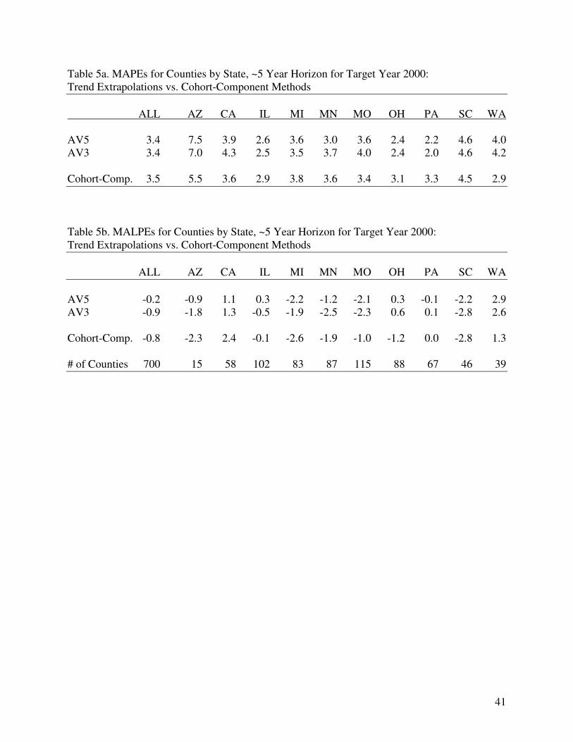
Table 5 presents forecast errors for county projections for the year 2000 for a sample of

10 states. The sources for the cohort-component projections are shown in Appendix B. Most of

the cohort-component projections use base data from the mid-1990s, resulting in a projection

horizon of about 5 years. The base data for the trend extrapolation methods include total

population from the 1980 and 1990 censuses, as well as revised 1985 intercensal and original

17

1995 postcensal estimates, all from the US Census Bureau. Using the revised intercensal and the

original postcensal estimates reflect the data that would have been available had the trend

extrapolation projections been made at the time of the cohort-component projections. These base

data were used to produce three sets of projections, covering 1980–1995, 1985–1995, and 1990–

1995 base periods, from which an average was calculated. To keep the discussion succinct, only

results for AV5 and AV3 are reported for the trend models.

The data in Table 5 demonstrate that trend extrapolations produce projections of total

population with generally similar levels of precision and bias as cohort-component models. For

some states, the extrapolations perform better, while in others the cohort-component models

shine. The two trend extrapolation averages provide generally similar results, and while there are

differences by individual states, they are too small to be of importance. Thus, for counties, and at

least for short horizons, projections of total population made with simple trend extrapolation

techniques are comparable to those made with cohort-component models.

To broaden the number of projection horizons and target years, one has to turn to

projections for states, which have been produced by the US Census Bureau for some time. The

Census Bureau projections contain several series that include varying assumptions about fertility

and especially migration, which can be thought of as scenarios. In some years, the Census

Bureau also produced a series that assumed no interstate migration, which was for illustrative

purposes only and is not included here. The acronyms shown in Table 6 (e.g. I-B) are those

originally used by the Census Bureau. A description of the specific assumptions applied in the

Census Bureau projection series can be found in the Current Population Reports referenced in

Appendix B.


18

Table 6 shows forecast precision and bias for the two trend technique averages compared

to several series of Census Bureau cohort-component projections for 1970, 1980, 1990, and

2000. Four sets of 5-year projections, three sets of 15-year projections, and one set of 25-year

projections are examined. Base data used for the trend extrapolations are the two prior censuses

before each target year, plus original postcensal estimates for the launch year and revised

intercensal estimates for one of the three base years. As before, an average of the three base

period lengths is calculated and reported in the table. For example, a five year projection for

target year 1990 would use postcensal 1985 estimates for the launch year, and census counts for

1970 and 1980 as well as intercensal estimates for 1975 for the three base years used.

Compared to the county-level projections, there is more variability in the results among

the various methods. For the 5-year projections, the MAPEs and MALPEs are similar between

the extrapolation and cohort-component models for 1980 and 2000, while the Census Bureau

projections are slightly more accurate for 1970 and significantly more accurate for 1990. One

should note, though, that the Census Bureau projections for 1990 start with a 1988 launch year,

and are thus really a two-year projection. For the longer range projections, the two types of

methods provide similar results, with the trend models at times outperforming the cohort-

component models both in terms of precision and bias. The data in Table 6 also demonstrate that

bias is essentially unpredictable: of the 5-year projections, all extrapolation methods and all

cohort-component series for 1970 and 1990 turned out too high, while the opposite was the case

in 1980 and 2000. The main conclusion, once again, is that the two types of projection models

provide generally comparable results.

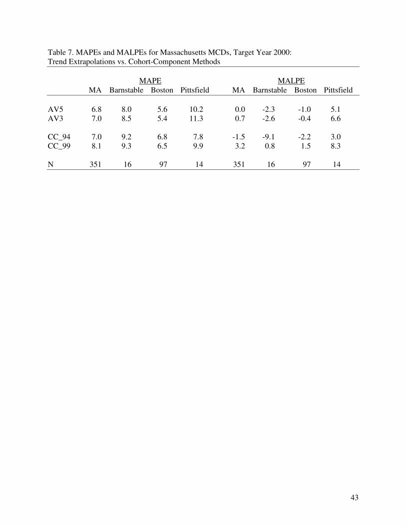
Because many forecasting projects in planning involve a specific area rather than all

states or all counties, a final comparison is presented for three metropolitan areas in

19

Massachusetts using minor civil division (MCD) data. The metropolitan areas were selected to

provide broad coverage by geography, population size, and population growth rate. The trend

extrapolations were calculated as before, using base data from 1980–1995. Also included are

results from two cohort-component projections made by Massachusetts state demographers for

the year 2000 that were released in 1994 and 1999 (see Appendix B for sources).


The results presented in Table 7 provide further evidence that simple projection

techniques are at least as accurate as more complex models for projections of total population.

Providing similar results for the state overall, for the Barnstable and Boston metropolitan areas

the trend extrapolations were slightly more precise than the cohort-component projections, while

for Pittsfield the cohort-component models, especially the one produced in 1994, produced

smaller errors. The data in Table 7 also nicely illustrate the general error structure of projections

by size and growth rate. Of the three metro areas, MCDs in Boston have the largest average

population size and generally low rates of population growth, resulting in the smallest forecast

errors. The largest errors for the trend extrapolations and the 1999 cohort-component projections

are recorded in Pittsfield, which has MCDs with the lowest average population size, and which

was the only metro area to decline in population from 1995 to 2000. Barnstable (Cape Cod) falls

in between, having MCDs with high growth rates but also larger average population sizes.

Discussion and Conclusion

Planners pursuing population projections face many decisions. First and foremost is the choice of

projection techniques, which range from simple trend extrapolations to more complex cohort-

component and structural models. Once chosen, the analyst then has to decide which base data to

20

use, how to form assumptions, how to treat special populations, etcetera. All too often, these

decisions are based on incomplete information, misconceptions, or legacy. So how should a

practitioner approach the forecasting process? If we assume that the ultimate purpose of a

population forecast is to provide a realistic picture of likely future population change, then a

concern about forecast accuracy is warranted. However, for planners this ideal of value-neutral

analytical forecasting has to be reconciled with the realities of the planning process where

forecasts also need to be evaluated with respect to their credibility with policy makers and the

public (Isserman 2007; Klosterman 2007). Because forecasting does not occur in a vacuum, the

issues of technique versus advocacy, of pure versus normative forecasting, need to be considered

(Skaburskis and Teitz 2003; Wachs 1986, 1989, 2001). Finally, there is the role of community

involvement that shapes forecasts produced by planners (for a summary see Hopkins and Zapata

2007). This study, while acknowledging the constraints of forecasting in planning practice, has

focused on the more technical aspects of model specification that planners need to make for each

forecasting project. These have important consequences on the outcome, and without a proper

understanding of the general characteristics of forecast error, projections remain a black box

open to misunderstandings and potential misuse.

The study pursued three primary objectives. It first examined the relationship between the

length of the base period and the length of the projection horizon with respect to projection

accuracy. This is a decision planners have to make at the beginning of each forecasting project,

and it is an issue that has received surprisingly little attention in the literature. The main finding

of this paper is that while the length of the base period beyond 10 years has only a limited impact

on projection precision, choosing an appropriate base period nevertheless demands attention,

21

because some projection techniques – the exponential model being a prime example – can

quickly lead to unrealistic forecasts.

The second objective of the analysis was to assess typical forecast errors for counties.

The aggregate analysis revealed that forecast precision decreases about linearly with increases in

the projection horizon. The length of the projection horizon had no consistent impact on bias.

The disaggregate analysis showed that both size and growth impact forecast precision. As

expected, projections become more precise with increasing population size. However, most of

the improvement comes at fairly low size levels. Indeed, it could be argued that for all but the

smallest areas size alone is only a limited indicator of forecast precision and that growth

dynamics are of greater importance. With respect to the latter, the study revealed a u-shaped

relationship: forecast precision is lowest for areas that are declining or growing rapidly and

highest for areas with little change in either direction over the base period.

In addition to variations in precision, the forecasts also revealed differences in bias by

growth category, whereas population size had no consistent impact. Counties that experienced

population declines over the base period tend to be under-projected while those that grew rapidly

are projected too high. The more rapidly the population declined or increased over the base

period, the more negative or positive the bias of the ensuing projections. This result underscores

the tendency of population growth patterns to moderate over time and lends strong support to the

notion of a regression towards the mean (Beaumont and Isserman 1987; Smith 1987). It should

be kept in mind when forming assumptions; otherwise, high growth rates experienced in the

recent past may be assumed to continue for too long, leading to unrealistically high forecasts.

These results can be considered benchmarks that are useful for planning purposes. For

example, as Table 3a illustrated, for small areas with a population of less than 2,500 people, a

22

twenty year projection will result in a forecast error of about 40%, which can make a big

difference when planning for future infrastructure projects. Uncertainty of that kind is

unfortunate but needs to be considered. It demonstrates that it is imperative that the analyst pays

special attention when projecting the population of small areas, areas undergoing rapid

population change, and when making longer-term projections. While projecting small and/or

rapidly changing places will always be a challenge, a careful choice of methods, base data, and

assumptions, when combined with the application of local knowledge, will lead to the best

possible projection outcomes.

The third focus of the paper was on forecast error by forecast technique. For that purpose,

individual trend extrapolation techniques were compared to averages, and trend extrapolations

were further checked against cohort-component models. With respect to the former, the various

averages led to promising results, i.e. to projections with higher precision and lower bias than

many of the individual extrapolation techniques. Averaging also worked well when deciding

among base periods. Furthermore, averaging works not only for trend extrapolation techniques

but can also be useful in a cohort-component setting when deciding which demographic rates to

choose (Isserman 1993). For example, a recent set of county population projections by race and

Hispanic origin for Minnesota employed a cohort-component model in which two different

methods of projecting migration were averaged (Minnesota State Demographic Center 2005).

The generally good performance of averaging raises the question why these techniques

are so seldom employed in actual population forecasting. Booth (2006, 570), in a review of the

past quarter century of demographic forecasting, cites several studies that have advocated

combining forecasts, yet states that “the idea has not been embraced.” Why not? Averaging

23

techniques are not always appropriate, and their composition should be carefully considered, but

the empirical evidence clearly supports their increased usage.

With respect to the choice of projection type, the cohort-component model has become

the de-facto standard, being regularly implemented for areas where simpler techniques, such as

trend extrapolations, might be just as suitable. As the comparison of the two projection model

types has shown, there were few instances where the more complex techniques outperformed the

extrapolations. But why is it that a simple technique such as the linear trend model provides

projections that are as accurate, on average, as those derived from more sophisticated techniques

such as cohort-component models that specifically account for the demographic processes of

births, deaths, and migration by which a population changes? Reasons include that projecting

fertility, mortality, and migration rates (or structural variables) are as difficult as, or even more

difficult than, projecting changes in total population; because more complex techniques require

detailed input data which may not be available or reliable; and because there exists some

irreducible level of uncertainty about the future that no method, however sophisticated, can

overcome time and again (Smith, Tayman, and Swanson 2001). According to Pant and Starbuck

(1990, 442), “a general law seems to be at work: more complex, subtle, or elegant techniques

give no greater accuracy than simple, crude, or naïve ones. More complex methods might

promise to extract more information from data, but such methods also tend to mistake noise for

information. As a result, more complex methods make more serious errors, and they rarely yield

the gains they promised.”

This does not mean that simple techniques are always appropriate, and informed

judgment is needed to determine when and how these methods can best be applied (Smith 1997).

Furthermore, there are situations where a cohort-component model would be advisable, e.g.

24

when demographic characteristics are needed such as when projecting the need for schools,

hospitals, nursing homes, or other facilities that serve specific segments of a population (for an

evaluation of the accuracy of population projections by age see Smith and Tayman 2003); or a

structural model, which is useful for evaluating scenarios and for linking projections to changes

in employment, transportation, and land use patterns, which are often important to planners

(Smith, Tayman, and Swanson 2001; Tayman 1996b).

This raises the question why a practitioner should bother to deal with trend extrapolation

methods at all, and not simply use cohort-component methods for forecasting projects that

require demographic characteristics. Yet it can be argued that trend models are useful even when

demographic characteristics are also required. For small areas the necessary input data for a

cohort-component or structural model are often not available. Even if they can be obtained, they

are seldom reliable, requiring numerous adjustments; and even when the data are of sufficient

quality, the practitioner still has to make choices regarding which variables to include in the

model. Furthermore, trend methods can easily incorporate the most recent estimates, while the

inputs required for cohort-component and structural models often lag in time. Perhaps the biggest

advantage of trend models is that they reduce the potential for unintentionally biasing the

projections, which can happen quite quickly during the assumption specification stage of more

complex models. Using averages of various trend techniques and base periods, one is more likely

to get a neutral forecast of total population, especially for small areas. The needed demographic

characteristics can then be obtained with cohort-component or structural techniques that are

controlled to the previously produced population totals. At the very least, the trend projections

provide an additional perspective, i.e. population figures that can be compared to results obtained

with other models. Trend extrapolations are easy enough to implement that the benefits of their

25

use should outweigh any extra effort. Following Smith, Tayman, and Swanson (2001), Figure 2

provides a brief summary that compares the respective strengths and weaknesses of the various

types of projection methods.

[Figure 2 about here.]

Advancing our knowledge about population projections is important, and so is research

that further refines the methods used. Using sophisticated projection models is popular, because

it conveys professionalism. Yet, as Skaburskis (1995: 200) warns, “the allure of large models

may be due to our wanting more certainty when it is most unattainable. To fall for the allure is to

decrease the thoughtfulness of planning decisions.” Based on the results of this study, one can

question whether the limited time and resources many practitioners have when projecting future

populations might not be better served by paying more attention to factors that actually make a

difference. Dealing with boundary changes, cleaning up and checking the reliability of the data,

and accounting for special events come to mind in this regard. These are particularly important

for small areas, and can have a major impact on forecast error. Once data quality is established,

one should think carefully about the assumptions made about future population trends, because

the core assumptions underlying each population forecast tend to be more important on the

outcome than the methods used (Ascher 1978). Finally, while all projections involve some

judgments, it is important to explain the reasoning for making specific choices in the projection

documentation (Pittenger 1977).

Calculations of future populations are only one aspect of the planning process, albeit an

important one. Planners are in a unique position not only to project the future but also to shape it.

Myers (2001, 394) urged that planners “need to become much more sophisticated in the use of

projections than they have in the past if they are to reclaim their leadership of the future.”

26

Projections inevitably involve many unknowns. We will never be able to perfectly forecast a

population all of the time. Nevertheless, concentrating on those factors that have been found to

make a difference will lead to better projections. The analyses presented in this paper with

respect to model choice and other specification issues, when considered within the social,

political, and economic contexts of the areas being projected, provide planners with a foundation

for making those informed choices.

27

References

Ahlburg, D. 1995. Simple versus complex models: Evaluation, accuracy, and combining.

Mathematical Population Studies 5: 281–290.

Alho, J., and B. Spencer. 1997. The practical specification of the expected error of population

forecasts. Journal of Official Statistics 13: 203–225.

Armstrong, S. 2001. Combining forecasts. In Principles of forecasting: A handbook for

researchers and practitioners, edited by S. Armstrong, 417–439. Norwell, MA: Kluwer.

Ascher, W. 1978. Forecasting: An appraisal for policy makers and planners. Baltimore, MD:

Johns Hopkins University Press.

Beaumont, P., and A. Isserman. 1987. Comment on “Tests of forecast accuracy and bias for

county population projections,” by S. Smith. Journal of the American Statistical Association

82: 1004–1009.

Booth, H. 2006. Demographic forecasting: 1980–2005 in review. International Journal of

Forecasting 22: 547–581.

Clemen, R. 1989. Combining forecasts: A review and annotated bibliography. International

Journal of Forecasting 5: 559–583.

Federal-State Cooperative for Population Projections. 1997. Unpublished survey

Flyvbjerg, B, M. Skamris Holm, and S. Buhl. 2005. How (in)accurate are demand forecasts in

public works projects? The case of transportation. Journal of the American Planning

Association 71: 131–146.

Forstall, R. 1996. Population of states and counties of the United States: 1790 to 1990.

Washington, DC: US Census Bureau.

28

Hopkins, L., and M. Zapata, ed. 2007. Engaging the future: Forecasts, scenarios, plans, and

projects. Cambridge, MA: Lincoln Institute of Land Policy.

Isserman, A. 1977. The accuracy of population projections for subcounty areas. Journal of the

American Institute of Planners 43: 247–259.

–––––. 1984. Projection, forecast, and plan: On the future of population forecasting. Journal of

the American Planning Association 50: 208–221.

–––––. 1985. Dare to plan: An essay on the role of the future in planning practice and education.

Town Planning Review 56: 483–491.

–––––. 1993. The right people, the right rates: Making population estimates and forecasts with an

interregional cohort-component model. Journal of the American Planning Association 59:

45–64.

–––––. 2007. Forecasting to learn how the world can work. In Engaging the future: Forecasts,

scenarios, plans, and projects, edited by L. Hopkins and M. Zapata, 175–197. Cambridge,

MA: Lincoln Institute of Land Policy.

Keyfitz, N. 1972. On population forecasting. Journal of the American Statistical Association 67:

347–363.

–––––. 1981. The limits of population forecasting. Population and Development Review 7: 579–

593.

Klosterman, R. 2007. Deliberating about the future. In Engaging the Future: Forecasts,

Scenarios, Plans, and Projects, edited by L. Hopkins and M. Zapata, 199–219. Cambridge,

MA: Lincoln Institute of Land Policy.

Long, J. 1995. Complexity, accuracy, and utility of official population projections. Mathematical

Population Studies 5: 203–216.

29

Mahmoud, E. 1984. Accuracy in forecasting: A survey. Journal of Forecasting 3: 139–159.

Makridakis, S. 1986. The art and science of forecasting: An assessment and future directions.

International Journal of Forecasting 2: 15–39.

Makridakis, S., A. Andersen, R. Carbone, R. Fildes, M. Hibon, R. Lewandowski, J. Newton, E.

Parzen, and R. Winkler. 1982. The accuracy of extrapolation (time series) methods: Results

of a forecasting competition. Journal of Forecasting 1: 111–153.

Makridakis, S., and M. Hibon. 1979. Accuracy of forecasting: An empirical investigation.

Journal of the Royal Statistical Society A 142: 97–145.

Makridakis, S., S. Wheelwright, and R. Hyndman. 1998. Forecasting: Methods and applications.

New York, NY: Wiley.

Mentzer, J., and K. Kahn. 1995. Forecasting technique familiarity, satisfaction, usage, and

application. International Journal of Forecasting 14: 465–476.

Minnesota State Demographic Center. 2005. Minnesota population projections by race and

Hispanic origin 2000–2030. St. Paul, MN: Minnesota Department of Administration.

Murdock, S., L. Leistritz, R. Hamm, S.-S. Hwang, and B. Parpia. 1984. An assessment of the

accuracy of a regional economic-demographic projection model. Demography 21: 383–404.

Murdock, S., R. Hamm, P. Voss, D. Fannin, and B. Pecotte. 1991. Evaluating small-area

population projections. Journal of the American Planning Association 57: 432–443.

Myers, D. 2001. Demographic futures as a guide to planning. Journal of the American Planning


Myers, D., and A. Kitsuse. 2000. Constructing the future in planning: a survey of theories and

tools. Journal of Planning Education and Research 19: 221–231.

30

Pant, N., and W. Starbuck. 1990. Innocents in the forest: Forecasting and research methods.

Journal of Management 16: 433–460.

Pittenger, D. 1977. Population forecasting standards: Some considerations concerning their

necessity and content. Demography 14: 363–368.

Rayer, S. 2004. Assessing the accuracy of trend extrapolation methods for population

projections: The long view. Paper presented at the annual meeting of the Southern

Demographic Association, Hilton Head Island, SC, October.

–––––. 2007. Population forecast accuracy: Does the choice of summary measure of error

matter? Population Research and Policy Review 26: 163–184.

Sawicki, D. 1989. Demographic analysis in planning: A graduate course and an alternative

paradigm. Journal of Planning Education and Research 9: 45–56.

Shryock, H., J. Siegel, and Associates. 1976. The methods and materials of demography.

Orlando, FL: Academic Press.

Skaburskis, A. 1995. Resisting the allure of large projection models. Journal of Planning

Education and Research 14: 191–202.

Skaburskis, A., and M. Teitz. 2003. Forecasts and outcomes. Planning Theory & Practice 4:

429–442.

Smith, S. 1987. Tests of forecast accuracy and bias for county population projections. Journal of

the American Statistical Association 82: 991–1003.

–––––. 1997. Further thoughts on simplicity and complexity in population projection models.

International Journal of Forecasting 13: 557–565.

Smith, S., and M. Shahidullah. 1995. An evaluation of population projection errors for census

tracts. Journal of the American Statistical Association 90: 64–71.

31

Smith, S., and T. Sincich. 1988. Stability over time in the distribution of population forecast

errors. Demography 25: 461–474.

–––––. 1990. The relationship between the length of the base period and population forecast

errors. Journal of the American Statistical Association 85: 367–375.

–––––. 1991. An empirical analysis of the effect of length of forecast horizon on population

forecast errors. Demography 28: 261–274.

–––––. 1992. Evaluating the forecast accuracy and bias of alternative population projections for

states. International Journal of Forecasting 8: 495–508.

Smith, S., and J., Tayman. 2003. An evaluation of population projections by age. Demography

40: 741–757.

Smith, S., J. Tayman, and D. Swanson. 2001. State and local population projections:

Methodology and analysis. New York, NY: Kluwer Academic/Plenum Publishers.

Stoto, M. 1983. The accuracy of population projections. Journal of the American Statistical


Tayman, J. 1996a. The accuracy of small area population forecasts based on a spatial interaction

land use modeling system. Journal of the American Planning Association 62: 85–98.

–––––. 1996b. Forecasting, growth management, and public policy decision making. Population

Research and Policy Review 15: 491–508.

Tayman, J., E. Schafer, and L. Carter. 1998. The role of population size in the determination and

prediction of population forecast errors: An evaluation using confidence intervals for

subcounty areas. Population Research and Policy Review 17: 1–20.

Wachs, M. 1986. Technique vs. advocacy in forecasting: A study of rail rapid transit. Urban

Resources 4: 23–30.

32

–––––. 1989. When planners lie with numbers. Journal of the American Planning Association

55: 476–479.

–––––. 2001. Forecasting versus envisioning: A new window on the future. Journal of the

American Planning Association 67: 367–372.

Webby, R., and M. O’Connor. 1996. Judgemental and statistical time series forecasting: A

review of the literature. International Journal of Forecasting 12: 91–118.

White, H. 1954. Empirical study of the accuracy of selected methods of projecting state

populations. Journal of the American Statistical Association 49: 480–498.

Wilson, T., and P. Rees. 2005. Recent developments in population projection methodology: A

review. Population, Space and Place 11: 337–360.

Yokum, T., and S. Armstrong. 1995. Beyond accuracy: Comparison of criteria used to select

forecasting methods. International Journal of Forecasting 11: 591–597.

33

Appendix A: Trend Extrapolation Techniques

Simple Methods

LIN: In the linear extrapolation technique, it is assumed that the population will increase

(decrease) by the same number of persons in each future decade as the average per decade

increase (decrease) observed during the base period:

Pt = Pl + (x / y) * (Pl – Pb),

where Pt is the population in the target year, Pl is the population in the launch year, Pb is the

population in the base year, x is the number of years in the projection horizon, and y is the

number of years in the base period.

EXP: In the exponential technique, it is assumed that the population will grow (decline) by the

same rate in each future decade as it did, per decade, during the base period:

Pt = Pl erx, r = [ln (Pl / Pb)] / y,

where e is the base of the natural logarithm and ln is the natural logarithm.

Ratio Methods

The share-of-growth, shift-share, and constant-share techniques require an independent national

projection for the target year population. These were produced by applying the linear and

exponential trend extrapolation techniques to the national population for each of the 63

projection horizon / base period combinations. To flatten out the discrepancies between the linear

and exponential methods, an average of the two techniques was then calculated and used for the

three ratio methods.

34

Ratio methods express the population (or population change) of a smaller area as a

proportion of the population (or population change) of a larger area the smaller area is located in.

In the following formulas, lowercase letters denote county-level values, and uppercase letters

denote national-level values. The same formulas can be applied to other areas of geography as

well, such as when making projections for census tracts, where the lowercase letters would then

denote the census tract and uppercase letters would refer to the county.

SHR: In the share-of-growth technique, it is assumed that a county’s share of national population

growth will be the same over the projection horizon as it was during the base period:

Pt = Pl + [(Pl – Pb) / (Pl – Pb)] * (Pt – Pl)

SFT: In the shift-share technique, it is assumed that the average per decade change in each

county’s share of the national population observed during the base period will continue

throughout the projection horizon:

Pt = Pt * [Pl / Pl + (x / y) * (Pl / P

l – Pb / Pb)]

COS: In the constant-share technique, it is assumed that a county’s share of the national

population will be the same in the target year as it was in the launch year:

Pt = (Pl / Pl) * Pt

35

Appendix B:

Sources for County Cohort-Component Projections Used in Table 5

Arizona, 1997, July 1, 1997 to July 1, 2050 Arizona county population projections. Arizona

Department of Economic Security, Research Administration, Population Statistics Unit.

California, 1998, County population projections with age, sex and race/ethnic detail. State of

California, Department of Finance.

Illinois, 1997, Illinois population trends 1990 to 2020. Treadway R, Delbert E, State of Illinois.

Michigan, 1996, Preliminary population projections to the year 2020 for Michigan by counties.

Office of the State Demographer, State Budget Office, Michigan Information Center.

Minnesota, 1998, Faces of the future: Minnesota county population projections 1995–2025.

Minnesota Planning, State Demographic Center.

Missouri, 1999, Projections of the population of Missouri counties by age and sex: 1990 to 2025.

Missouri Office of Administration, Division of Budget and Planning.

Ohio, 1997, Population projections: Ohio and counties by age and sex, 1990 to 2015. Ohio

Department of Development, Office of Strategic Research.

Pennsylvania, 1998, Detailed county population projections: 2000 to 2020. Pennsylvania State

Data Center, Institute of State and Regional Affairs, Penn State Harrisburg.

South Carolina, 1998, Population projections at five year intervals for South Carolina counties:

1990–2015. South Carolina Budget & Control Board, Office of Research and Statistics.

Washington, 1995, Washington state county growth management population projections: 1995

to 2020. Office of Financial Management, State of Washington.

36

Sources for State Cohort-Component Projections Used in Table 6

US Census Bureau, 1967, Illustrative projections of the population of states 1970 to 1985.

Current Population Reports, Series P-25, No. 362.

US Census Bureau, 1978, Illustrative projections of state populations: 1975 to 2000. Current

Population Reports, Series P-25, No. 735.

US Census Bureau, 1990, Projections of the population of states by age, sex, and race: 1989 to

2010. Current Population Reports, Series P-25, No. 1053.

US Census Bureau, 1997, Population projections: states, 1995–2025. Current Population

Reports, Series P-25, No. 1131.

Sources for Sub-county Cohort-Component Projections Used in Table 7

Massachusetts, 1994, Projections of the Population, Massachusetts Cities and Towns, Year 2000

and 2010. Massachusetts Institute for Social and Economic Research, University of

Massachusetts.

Massachusetts, 1999, Projections of the Population, Massachusetts Cities and Towns, Year 2000

and 2010. Massachusetts Institute for Social and Economic Research, University of

Massachusetts.

37

Table 1a. MAPE by Projection Horizon and Base Period (1960–2000 Target Years)

Horizon Base LIN SHR SFT EXP COS AV5 AV3

10 10 10.5 10.9 12.7 11.0 14.1 9.8 10.6

10 20 9.8 10.2 12.4 10.1 13.6 9.5 9.8

10 30 10.0 10.4 13.4 10.3 13.5 9.8 10.0

10 Ave 9.6 9.9 12.1 9.9 13.7 9.3 9.6

20 10 20.7 22.0 27.8 23.7 27.3 19.9 20.9

20 20 19.4 20.6 27.4 22.7 27.4 19.4 19.5

20 30 19.8 21.0 29.5 22.4 27.5 19.8 19.8

20 Ave 18.8 19.9 26.5 21.7 27.3 18.7 18.9

30 10 32.8 35.6 47.4 4,488.7 43.7 921.4 33.4

30 20 30.6 33.3 45.7 57.7 42.9 34.7 31.2

30 30 31.0 34.0 48.3 70.7 42.3 38.2 32.0

30 Ave 30.1 32.8 45.6 1,537.3 42.9 330.3 30.8

Table 1b. MALPE by Projection Horizon and Base Period (1960–2000 Target Years)

Horizon Base LIN SHR SFT EXP COS AV5 AV3

10 10 -3.0 -3.0 -5.0 -0.2 6.6 -0.9 -2.5

10 20 -3.2 -3.1 -6.0 -0.2 6.1 -1.3 -2.6

10 30 -3.9 -3.7 -7.9 -0.4 6.0 -2.0 -3.1

10 Ave -3.4 -3.3 -6.3 -0.3 6.2 -1.4 -2.7

20 10 -3.7 -3.6 -9.3 5.0 15.6 0.8 -2.2

20 20 -5.4 -5.3 -13.7 4.1 16.0 -0.9 -3.8

20 30 -5.9 -5.7 -16.6 3.4 15.9 -1.8 -4.2

20 Ave -5.0 -4.9 -13.5 4.1 15.9 -0.7 -3.4

30 10 -8.2 -8.0 -20.1 4,458.1 29.3 890.2 -5.3

30 20 -8.1 -7.9 -23.0 29.1 28.5 3.7 -5.2

30 30 -6.1 -5.3 -22.5 43.4 27.7 7.4 -2.8

30 Ave -7.7 -7.3 -22.9 1,510.2 28.5 300.2 -4.5

38

Table 2a. MAPE by Projection Horizon and Growth Rate, 20 Year Base Period

Horizon Growth Rate LIN SHR SFT EXP COS AV5 AV3

20 < -15% 49.1 56.6 86.1 29.0 45.7 36.3 44.5

20 -15% to -5% 18.3 20.6 40.5 15.9 39.3 16.2 18.1

20 -5% to 5% 14.2 14.3 18.9 14.2 27.2 14.4 14.2

20 5% to 15% 17.3 17.9 17.4 18.2 21.0 18.0 17.8

20 15% to 30% 20.9 22.4 23.8 26.6 20.6 22.4 22.3

20 > 30% 30.6 32.8 38.5 107.8 29.3 43.7 33.6

Table 2b. MALPE by Projection Horizon and Growth Rate, 20 Year Base Period

Horizon Growth Rate LIN SHR SFT EXP COS AV5 AV3

20 < -15% -48.9 -56.6 -86.1 -27.2 41.2 -35.5 -44.3

20 -15% to -5% -13.6 -17.0 -39.8 -9.3 37.4 -8.5 -13.3

20 -5% to 5% -2.0 -2.1 -13.1 -1.7 23.8 1.0 -1.9

20 5% to 15% 2.2 4.3 1.3 5.2 10.8 4.8 3.9

20 15% to 30% 4.4 8.0 11.2 16.2 0.2 8.0 8.0

20 > 30% 5.1 10.6 21.1 98.7 -14.2 24.2 12.2

39

Table 3a. MAPE by Projection Horizon and Population Size, 20 Year Base Period

Horizon Population Size LIN SHR SFT EXP COS AV5 AV3

20 < 2,500 41.0 43.9 54.8 51.4 45.3 39.2 40.2

20 2,500 - 7,500 28.6 31.5 44.5 54.8 37.8 32.3 29.1

20 7,500 - 15,000 21.4 23.1 32.9 27.0 33.4 22.0 21.7

20 15,000 - 30,000 17.3 18.2 24.8 19.8 25.3 17.4 17.6

20 30,000 - 100,000 16.1 16.8 19.8 21.5 20.7 16.9 16.7

20 > 100,000 15.7 16.9 19.0 27.4 19.2 17.6 17.0

Table 3b. MALPE by Projection Horizon and Population Size, 20 Year Base Period

Horizon Population Size LIN SHR SFT EXP COS AV5 AV3

20 < 2,500 -16.2 -17.8 -30.0 12.2 23.6 -5.6 -13.1

20 2,500 - 7,500 -6.0 -7.0 -20.0 29.9 28.0 5.0 -3.6

20 7,500 - 15,000 -4.0 -4.7 -17.7 7.1 26.7 1.5 -2.7

20 15,000 - 30,000 -3.4 -3.1 -12.1 2.7 18.1 0.4 -2.2

20 30,000 - 100,000 -1.3 0.7 -2.1 9.0 7.2 2.7 1.0

20 > 100,000 0.7 4.1 6.6 19.9 -1.3 6.0 4.5

40

Table 4a. MAPE by Projection Horizon and Extrapolation Technique, 20 Year Base Period

Horizon LIN SHR SFT EXP COS AV5 AV3 C1 C2 C3 C4

10 10.5 10.9 13.0 11.7 14.3 10.5 10.6 10.3 10.1 11.1 11.1

20 19.7 21.1 28.2 27.2 27.8 20.6 20.2 18.2 18.5 21.2 21.3

30 31.0 34.0 46.9 79.7 43.8 39.6 32.1 27.6 28.4 33.7 33.5

Table 4b. MALPE by Projection Horizon and Extrapolation Technique, 20 Year Base Period

Horizon LIN SHR SFT EXP COS AV5 AV3 C1 C2 C3 C4

10 -1.6 -1.4 -4.2 2.1 7.3 0.5 -0.9 -2.5 -1.0 -0.3 -1.2

20 -3.2 -2.7 -10.9 10.0 17.6 2.2 -1.3 -3.9 -1.5 0.2 -2.4

30 -5.2 -4.3 -19.1 53.2 30.0 10.9 -1.8 -4.9 -2.1 1.5 -3.9

Note: Composite averages were created from the following techniques

C1 = EXP if growth rate < -5%

= LIN if growth rate -5% to 15%

= COS if growth rate > 15%

C2 = EXP if growth rate < -5%

= LIN if growth rate > -5%

C3 = Average of LIN/SHR/EXP/COS if growth rate < -5%

= Average of LIN/SHR/SFT/EXP if growth rate -5% to 15%

= Average of LIN/SHR/SFT/COS if growth rate > 15%

C4 = Average of LIN/SHR/EXP if growth rate < 5%

= Average of LIN/SHR/SFT if growth rate 5% to 15%

= Average of LIN/SHR/COS if growth rate > 15%

41

Table 5a. MAPEs for Counties by State, ~5 Year Horizon for Target Year 2000:

Trend Extrapolations vs. Cohort-Component Methods

ALL AZ CA IL MI MN MO OH PA SC WA

AV5 3.4 7.5 3.9 2.6 3.6 3.0 3.6 2.4 2.2 4.6 4.0

AV3 3.4 7.0 4.3 2.5 3.5 3.7 4.0 2.4 2.0 4.6 4.2

Cohort-Comp. 3.5 5.5 3.6 2.9 3.8 3.6 3.4 3.1 3.3 4.5 2.9

Table 5b. MALPEs for Counties by State, ~5 Year Horizon for Target Year 2000:


ALL AZ CA IL MI MN MO OH PA SC WA

AV5 -0.2 -0.9 1.1 0.3 -2.2 -1.2 -2.1 0.3 -0.1 -2.2 2.9

AV3 -0.9 -1.8 1.3 -0.5 -1.9 -2.5 -2.3 0.6 0.1 -2.8 2.6

Cohort-Comp. -0.8 -2.3 2.4 -0.1 -2.6 -1.9 -1.0 -1.2 0.0 -2.8 1.3

# of Counties 700 15 58 102 83 87 115 88 67 46 39

42

Table 6. MAPEs and MALPEs for States: Trend Extrapolations vs. Cohort-Component Methods

MAPE MALPE

Horizon 5 5 5 5 5 5 5 5

Target Year 1970 1980 1990 2000 1970 1980 1990 2000

AV5 3.9 4.3 4.3 2.4 3.1 -2.1 2.6 -1.7

AV3 3.7 3.7 4.4 2.5 2.8 -2.0 2.6 -1.9

I-B 3.3 1.6

II-B 3.3 1.6

I-D 3.1 0.3

II-D 3.0 0.4

II-A 4.6 -3.2

II-B 3.6 -2.5

A 1.6 0.9

B 2.1 1.3

C 1.6 0.9

A 2.5 -1.2

B 2.3 -1.4

MAPE MALPE

Horizon 15 15 15 25 15 15 15 25

Target Year 1980 1990 2000 2000 1980 1990 2000 2000

AV5 8.9 5.8 6.5 7.8 3.5 0.1 0.9 -1.9

AV3 8.5 5.0 7.4 7.2 2.4 -0.1 0.5 -2.6

I-B 9.6 3.2

II-B 9.8 3.7

I-D 9.1 -3.7

II-D 8.9 -3.2

II-A 6.4 10.1 -1.9 -6.6

II-B 5.5 8.8 -0.3 -4.5

A 7.7 -5.7

B 6.0 -3.2

C 6.6 -5.1

43

Table 7. MAPEs and MALPEs for Massachusetts MCDs, Target Year 2000:


MAPE MALPE

MA Barnstable Boston Pittsfield MA Barnstable Boston Pittsfield

AV5 6.8 8.0 5.6 10.2 0.0 -2.3 -1.0 5.1

AV3 7.0 8.5 5.4 11.3 0.7 -2.6 -0.4 6.6

CC_94 7.0 9.2 6.8 7.8 -1.5 -9.1 -2.2 3.0

CC_99 8.1 9.3 6.5 9.9 3.2 0.8 1.5 8.3

N 351 16 97 14 351 16 97 14

Figure 2. Comparison of Projection Methods

Extrapolation Cohort-Component Structural

Forecast Accuracy – – –

Political Acceptability – – –

Face validity – – –

Plausibility – – –

Cost of Production *** ** *

Timeliness *** ** *

Ease of Application *** ** *

Ease of Explanation *** ** *

Geographic Detail *** ** **

Demographic Detail * *** ***

Temporal Detail *** *** ***

Usefulness for Scenarios * ** ***

Note: *** good, ** average, * poor, – cannot generalize

population forecast errors: a primer for planners

Documents