population balance modeling of aerated stirred vessels

Population Balance Modeling of Aerated StirredVessels Based on CFD

Bart C. H. Venneker, Jos J. Derksen, and Harrie E. A. Van den AkkerKramers Laboratorium voor Fysische Technologie, Delft University of Technology,

2628 BW Delft, The Netherlands

A de®eloped model predicts local gas fraction and bubble-size distributions for turbu-( )lent gas dispersion in a stirred ®essel, based on the population balance equations PBE ,

with relations taken from literature for bubble coalescence and breakup deri®ed fromisotropic turbulence theory. The transport of bubbles throughout the ®essel is simulatedby a scaled single-phase flow field obtained by CFD simulations. Model predictions forthe gas fractions in pseudoplastic Xanthan solutions are compared with local measure-ments and agree well qualitati®ely. This formulation o®ercomes the necessity of choos-ing a constant bubble size throughout the domain, as is done in two-fluid models and is,therefore, more reliable in mass-transfer calculations.

Introduction

Stirred vessels are widely used, among other things, in pro-Ž .cess industries for bio chemical reactions involving more than

one phase. Equipped with an impeller revolving at high speedand operated in the turbulent flow regime, stirred vessels aregenerally considered useful devices for creating a large inter-facial contact area between the phases, thereby promotingmass transfer. Nowadays, however, awareness is growingamong chemical engineers that, under conditions typical ofcommercial operation, ‘‘intensity’’ and ‘‘quality’’ of flow, tur-bulent kinetic energy, turbulent eddies, volume fractions ofphases, concentrations of species, and interfacial contact areaare never uniformly distributed throughout the vessel. Largevalues of velocities, kinetic energy, and energy dissipation rateare found in the impeller region, while, near the walls andthe top of the vessel, the flow is often more quiescent. As aresult, in the case of multiple-phase reactors, the spatial dis-tribution of the phases may be very uneven; the same appliesto bubble and droplet sizes in aerated stirred vessels and inagitated liquid-liquid dispersion, respectively. Overall reactorefficiency might increase if, in the more quiescent regions ofa stirred vessel, a larger part of the interfacial mass transfercould be effected.

Correspondence concerning this article should be addressed to J. J. Derksen.Current address of B. C. H. Venneker: Laboratory for Materials Science, Delft

University of Technology, Delft, The Netherlands.

Current methods for designing and improving multiphasereactors, however, are predominantly based on empirical cor-relations for overall quantities such as power consumptionand mixing times. These correlations have several drawbacks:they do not reflect the details of the physics involved in masstransfer and are only applicable in the narrow range of oper-ating conditions for which they were determined. A new de-sign tool can be found in the use of computational fluid dy-

Ž .namics CFD techniques. The improvements attained overthe last three decades in the areas of turbulence modeling,grid-meshing, and numerical methods now make it possible

Ž .to perform reliable three-dimensional 3-D simulations, evenfor a difficult system as a stirred vessel.

In the case of multiphase flow, the situation is more com-plex. Transport equations for mass, momentum, and turbu-lence properties have to be solved for each individual phase.These equations, however, suffer from a lack of universalagreement as to a generally valid formulation of the interfa-cial transfer terms. In addition, turbulence of multiphaseflows is an area hardly covered by fundamental studies as toits dynamics. As the pertinent transport equations are highlycoupled and nonlinear, an efficient, yet robust, solution tech-nique for the resulting large sets of algebraic equations is not

Žreadily available Lathouwers and van den Akker, 1996; van.Santen et al., 1996 .

In general, the continuum phase is treated by an Eulerianapproach. For the dispersed phase, two options are available.

April 2002 Vol. 48, No. 4AIChE Journal 673

Ž .In case of very small loadings, the dispersed phase may berepresented by a finite number of particles the motion ofwhich is tracked in a Lagrangian manner. For high loading orif particle-particle interactions are dominant, the Eulerian

Žapproach is preferred, based on the two-fluid model Ishii,.1975 . Examples of the latter approach for the simulation of

two-phase stirred reactors can be found in Issa and GosmanŽ . Ž . Ž .1981 , Gosman et al. 1992 , Morud and Hjertager 1996 ,

Ž . Ž .Djebbar et al. 1996 , and Jenne and Reuss 1997 . An alter-native method, introduced by Bakker and van den AkkerŽ . Ž .1994 see also Bakker, 1992 , exploited a slip velocity modeland an effective coalescence-redispersion model with a viewto deriving a spatial gas fraction distribution from the single-phase flow field obtained via a CFD simulation. A commonfeature of all these models is the use of a single bubble size.While this may be a reasonable approach for noncoalescingmedia, in general this may limit the application of all thesemodels.

The objective of the present work is to develop a modelwhich is possible to obtain local bubble-size distributions, and,hence, local gas fractions and mass-transfer rates in an aer-ated stirred vessel. The model is formulated in terms of pop-

Ž .ulation balance equations PBEs and has been implementedŽ .by Venneker 1999 in the in-house code DAWN. Breakup

and coalescence of bubbles is modeled in a fundamental wayusing isotropic turbulence theory. One of the assumptionsmade in the model is that gas bubbles do not significantlyalter the flow field. Given a prediction of the single-phaseflow field, the flow field in gassed conditions can be obtained

Žby a scaling of the single-phase flow field with only the ex-.perimentally determined drop in power-consumption as a

parameter. We will call this 1.5-way coupling. This limits theŽ .application of this model to low gas loadings 0]5% , but it

offers a more accurate method to predict mass-transfer ratesthan the present two-fluid models.

General Formulation of the ModelPopulation balance equations

The key reason why fluid-particle systems may be modeledŽ .in terms of population balance equations PBEs is the dy-

namics of the particle-size distribution of interest. The dy-namics may only be due to processes by which particles grad-

Žually increase andror decrease in size such as in response to.variations in the chemical composition in the liquid phase ,

but also due to processes involving continuous interactionsŽbetween individual particles such as agglomeration, coales-

.cence, and breakup . Rather than following individual parti-cles, as is done in particle tracking, a continuum approachbased on particle statistics is pursued. The concept of PBE,

Ž .which was first presented by Hulburt and Katz 1964 , is nowbeing used in many applications, particularly in the field ofcrystallization, including the production of margarine. Fur-ther references on PBE can be found in the general review of

Ž .Ramkrishna 1985 , as well as in the review of the applicationof population balances to chemical reactors due to Ritchie

Ž .and Togby 1978 . The combination of PBEs and CFD is rel-atively new.

In general, the PBE is a balance equation of the numberdensity probability of some particle property. In the presentapplication, the particle property x is the number density

probability of particles with bubble size d, but one can alsothink of the particle age as a modeled property in order todetermine the residence time distribution.

The PBE in its most general form is given by RamkrishnaŽ .1985 as

n x , r , tŽ .q= ? xn x , r , t q= ? © n x , r , tŽ . Ž .˙x r p t

s B x , r , Y , t y D x , r , Y , t 1Ž . Ž . Ž .

Ž .in which n x, r, t is the number density probability of theproperty under consideration as function of the property vec-tor x, the physical position of the particle r and time t. x is˙the growth rate of the particle due to processes other thaninteraction with other particles, and © is the velocity of thepparticle. The continuous phase variables which may affect the

Ž .particle property, are represented by the vector Y r, t .Ž .On the righthand side of Eq. 1, B x, r, Y, t represents the

Ž . Ž .rate of production birth and D x, r, Y, t the rate of de-Ž . Ž .struction death of particles of a particular state x, r at

time t. In the case of bubble size as the particle property,bubbles of a certain diameter d are continuously formed byeither breakage of larger bubbles or coalescence of smallerbubbles. Similarly, bubbles of diameter d are continuouslydestroyed by breakage into smaller bubbles, and by coales-cence into larger ones. The functions that describe thesebreakup and coalescence processes have to be specified fur-ther. Their specific form may vary for different particle-fluidsystems and for the particle property under consideration.

Gas-Dispersion Modeling. In the case of gas-dispersionmodeling where the bubble diameter is the most importantbubble property, the following forms have been adopted for

Ž .the birth and death functions Tsouris and Tavlarides, 1994

1 d Y X Y X Y X XB d , t s p d , d h d , d n d , t n d , t d dŽ . Ž . Ž . Ž . Ž .H2 0

`X X X X Xq h d , d n d g d n d , t d d 2Ž . Ž . Ž . Ž . Ž .H

d

Y Ž 3 X 3.1r3in which d s d y d , and

`X X X XD d , t s n d , t p d , d h d , d n d , t d dŽ . Ž . Ž . Ž . Ž .H

0

q g d n d , t 3Ž . Ž . Ž .

Note that the dependency on r and Y has been dropped forbrevity only. The various parameters in Eqs. 2 and 3 relate tothe following physical mechanisms:

Ž X.h d, d : effective swept volume rate of bubbles of diame-X w 3 xter d colliding with bubbles of diameter d m rs

Ž X.p d, d : coalescence efficiency after collision betweenX w xbubbles of diameter d and d }

Ž . w xg d : breakage frequency of bubbles of diameter d 1rsŽ X. w xh d, d : daughter probability distribution 1rmŽ X.n d : number of bubbles formed from the breakage of a

X w xbubble diameter d }

April 2002 Vol. 48, No. 4 AIChE Journal674

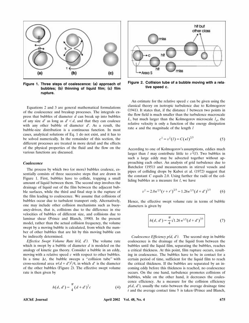
( )Figure 1. Three steps of coalescence: a approach of( ) ( )bubbles; b thinning of liquid film; c film

rupture.

Equations 2 and 3 are general mathematical formulationsof the coalescence and breakup processes. The integrals ex-press that bubbles of diameter d can break up into bubblesof any size dX as long as dX - d, and that they can coalescewith any other bubble of diameter dX. As a result, thebubble-size distribution is a continuous function. In mostcases, analytical solutions of Eq. 1 do not exist, and it has tobe solved numerically. In the remainder of this section, thedifferent processes are treated in more detail and the effectsof the physical properties of the fluid and the flow on thevarious functions are discussed.

CoalescenceŽ .The process by which two or more bubbles coalesce, es-

sentially consists of three successive steps that are drawn inFigure 1. First, bubbles have to collide, trapping a smallamount of liquid between them. The second step involves thedrainage of liquid out of the film between the adjacent bub-ble surfaces, while the third and final step is the rupture ofthe film leading to coalescence. We assume that collisions ofbubbles occur due to turbulent transport only. Alternatively,one may include other collision mechanisms such as buoy-ancy-driven, that is, collisions due to the difference in risevelocities of bubbles of different size, and collisions due to

Ž .laminar shear Prince and Blanch, 1990 . In the presentmodel, rather than the actual collision frequency, the volumeswept by a moving bubble is calculated, from which the num-ber of other bubbles that are hit by this moving bubble canbe indirectly determined.

( X)Effecti®e Swept Volume Rate h d, d . The volume ratewhich is swept by a bubble of diameter d is modeled on theanalogy of kinetic gas theory. Consider a bubble in an eddy,moving with a relative speed c with respect to other bubbles.In a time D t, the bubble sweeps a ‘‘collision tube’’ with

Ž X.2 Xcross-sectional area p dq d r4, in which d is the diameterŽ .of the other bubbles Figure 2 . The effective swept volume

rate is then given by

p 2X Xh d , d s dq d c 4Ž . Ž . Ž .4

Figure 2. Collision tube of a bubble moving with a rela-tive speed c.

An estimate for the relative speed c can be given using theclassical theory on isotropic turbulence due to KolmogorovŽ .1941 . It states that, if the distance l between two points inthe flow field is much smaller than the turbulence macroscaleL, but much larger than the Kolmogorov microscale l , thedrelative velocity is only a function of the energy dissipationrate e and the magnitude of the length l

2r32 2c s ® l sC e l 5Ž . Ž . Ž .

According to one of Kolmogorov’s assumptions, eddies much2Ž .larger than l may contribute little to ® l . Two bubbles in

such a large eddy may be advected together without ap-proaching each other. An analysis of grid turbulence due to

Ž .Batchelor 1951 and measurements in stirred vessels andŽ .pipes of colliding drops by Kuboi et al. 1972 suggest that

the constant C equals 2.0. Using further the radii of the col-liding bubbles as a measure for l, we have

2r3 2r3X X2 2r3 2r3® s2.0e r q r s1.26e dq d 6Ž . Ž . Ž .

Hence, the effective swept volume rate in terms of bubblediameters is given by

p 7r3X X1r3'h d , d s 1.26 e dq d 7Ž . Ž . Ž .4

( X)Coalescence Efficiency p d, d . The second step in bubblecoalescence is the drainage of the liquid from between thebubbles until the liquid film, separating the bubbles, reachesa critical thickness. At this point, film rupture occurs, result-ing in coalescence. The bubbles have to be in contact for acertain period of time, sufficient for the liquid film to reachthe critical thickness. If the bubbles are separated by an in-coming eddy before this thickness is reached, no coalescenceoccurs. On the one hand, turbulence promotes collisions ofbubbles, while on the other hand, it decreases the coales-cence efficiency. As a measure for the collision efficiencyŽ X.p d, d , usually the ratio between the average drainage time

Žt and the average contact time t is taken Prince and Blanch,


.1990

tXp d , d sexp y 8Ž . Ž .

t

Figure 1b shows the drainage of the liquid film betweentwo bubbles, which are trapped in an eddy with lifetime t .

Depending on the viscosities of the two phases and thepresence of surfactants, the drainage of the liquid film be-tween two bubbles is modeled in different ways. A useful,more precise conceptual picture is that, when two bubblesapproach one another, the interfaces flatten and give rise toa circular disc-like film of liquid in between. The liquid hasto drain from this disc when the flat interfaces get closer. Foran aqueous-air system, the bubble interfaces are deformableand fully mobile. Film drainage is controlled by inertia and

Ž .surface tension forces if Chesters, 1975

4m<1 9Ž .

rVr

in which V is the approach velocity of the two bubbles.A relation for the film thickness h can then be derived by

Žsolving Bernoulli’s equation for the disc Kirkpatrick and.Lockett, 1974

shs h exp y4 t 10Ž .0 2( r a Rc eq

in which R is the equivalent bubble radius, given byeq

2R s 11Ž .Xeq 1rr q1rr

for the coalescence between two unequally sized bubbles withradii r and rX. To calculate the drainage time, we need esti-mates for the initial film thickness h , for the radius of the0thinning disc a, and for the critical thickness h at which thecfilm ruptures.

Ž .Chesters 1975 gives an estimate for h , assuming that the0pressure generated between approaching spherical bubblesbecomes sufficiently high to cause substantial deformation

r V 2R2c eq

h s 12Ž .0 4s

Alternatively, a single value may be used for h irrespective0Ž .of bubble radius. For example, Kirkpatrick and Lockett 1974

used h s0.1 mm in all cases, which is considerably smaller0than predicted by Eq. 12.

The radius a actually is a function of time, which compli-cates the drainage equations substantially. Most authors,therefore, assume that deformation of the bubble surface oc-curs instantaneously and poses a relation for a. We used a

Ž .relation due to Chesters 1991

1r41r2 2r V RWe c eqas R s R 13Ž .eq eqž / ž /2 2s

This relation is based on the relative increase in surface area,and, hence, on the surface free energy. The approach velocityV may be set equal to ® given by Eq. 6.

Finally, for the critical film thickness h , an approach duecŽ .to Chesters 1991 is adopted that leads to the expression

1r3AReqh s 14Ž .c ž /8ps

with A the Hamaker constant.The drainage time in the case of deformable, fully mobile

interfaces is then given by

1 h0t s ln 15Ž .mob s ž /hc4 2( r a Rc eq

Ž .The average contact time t is given by Levich 1962 as

2r3Xdq dŽ .t s 16Ž .1r3e

So, the coalescence efficiency is obtained by substituting Eq.15 and 16 into 8.

BreakupBreakup of bubbles in a turbulent flow is caused by turbu-

lent eddies bombing the bubble surface. If the energy of theincoming eddy is sufficiently high to overcome the surfaceenergy, deformation of the surface is the result, which canfinally lead to the formation of two or more daughter bub-bles. For bubble breakup to occur, the sizes of the bombard-ing eddies have to be smaller than or equal to the bubblesize, since larger eddies only transport the bubble.

In order to model the breakup process, the following sim-Ž .plifications are generally made Luo and Svendsen, 1996 :

Ž .1 The turbulence is isotropic.Ž . Ž .2 Only binary breakage of a bubble is considered n s2 .Ž .3 The breakage volume ratio is a stochastic variable.Ž .4 The occurrence of breakup is determined by the en-

ergy level of the arriving eddy.Ž .5 Only eddies of a size smaller than or equal to the bub-

ble diameter can cause bubble breakup.The second and third simplification are supported by ex-

perimental observations on bubble breakage by Hesketh etŽ .al. 1991 .

( )Breakage Frequency g d . As stated above, for a bubble toŽ .break up, the colliding eddies must have 1 sufficient energy

Ž .to overcome the increase in surface energy, and 2 a size ofthe order of the bubble diameter. As a result, breakage fre-


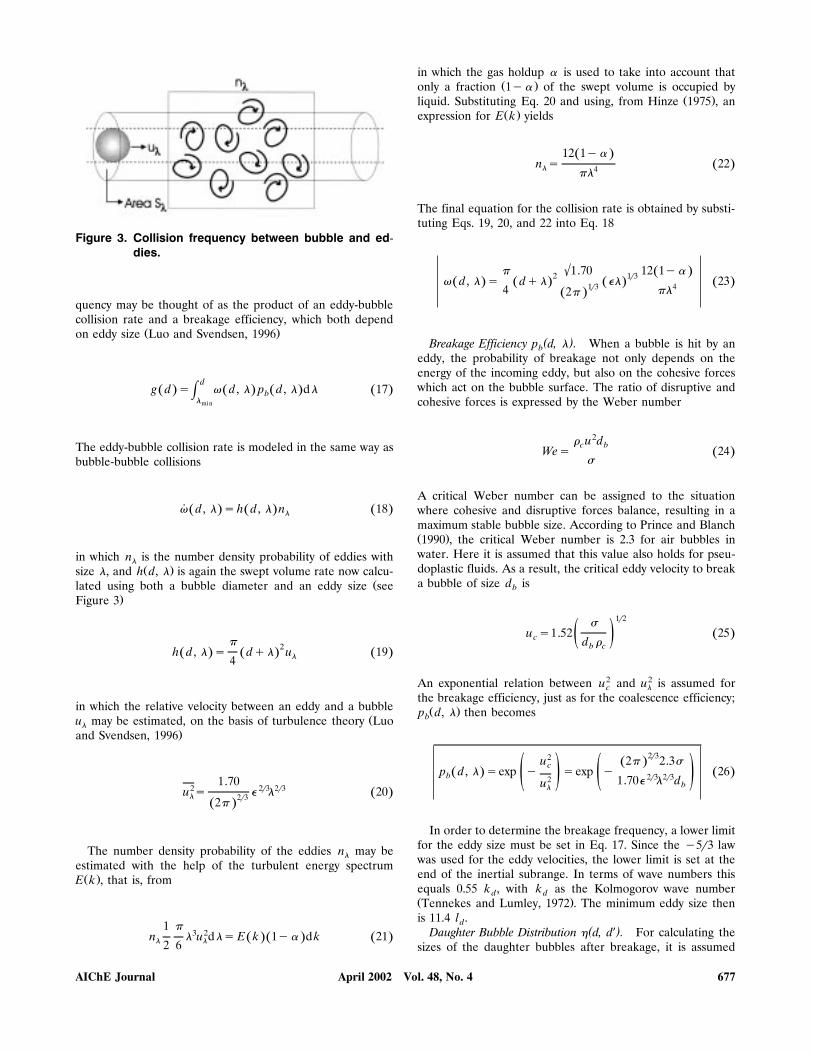
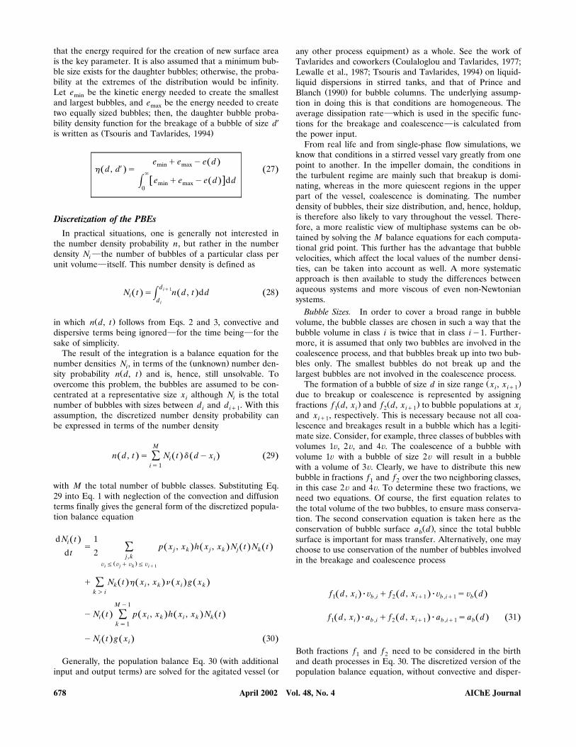
Figure 3. Collision frequency between bubble and ed-dies.

quency may be thought of as the product of an eddy-bubblecollision rate and a breakage efficiency, which both depend

Ž .on eddy size Luo and Svendsen, 1996

dg d s v d , l p d , l d l 17Ž . Ž . Ž . Ž .H b

lmin

The eddy-bubble collision rate is modeled in the same way asbubble-bubble collisions

v d , l s h d , l n 18Ž . Ž . Ž .˙ l

in which n is the number density probability of eddies withl

Ž .size l, and h d, l is again the swept volume rate now calcu-Žlated using both a bubble diameter and an eddy size see

.Figure 3

p 2h d , l s dq l u 19Ž . Ž . Ž .l4

in which the relative velocity between an eddy and a bubbleŽu may be estimated, on the basis of turbulence theory Luol

.and Svendsen, 1996

1.702 2r3 2r3u s e l 20Ž .l 2r32pŽ .

The number density probability of the eddies n may bel

estimated with the help of the turbulent energy spectrumŽ .E k , that is, from

1 p3 2n l u d ls E k 1y a d k 21Ž .Ž . Ž .l l2 6

in which the gas holdup a is used to take into account thatŽ .only a fraction 1y a of the swept volume is occupied by

Ž .liquid. Substituting Eq. 20 and using, from Hinze 1975 , anŽ .expression for E k yields

12 1y aŽ .n s 22Ž .l 4pl

The final equation for the collision rate is obtained by substi-tuting Eqs. 19, 20, and 22 into Eq. 18

'p 1.70 12 1y aŽ .2 1r3v d , l s dq l el 23Ž . Ž . Ž . Ž .1r3 44 pl2pŽ .

( )Breakage Efficiency p d, l . When a bubble is hit by anbeddy, the probability of breakage not only depends on theenergy of the incoming eddy, but also on the cohesive forceswhich act on the bubble surface. The ratio of disruptive andcohesive forces is expressed by the Weber number

r u2dc bWes 24Ž .

s

A critical Weber number can be assigned to the situationwhere cohesive and disruptive forces balance, resulting in amaximum stable bubble size. According to Prince and BlanchŽ .1990 , the critical Weber number is 2.3 for air bubbles inwater. Here it is assumed that this value also holds for pseu-doplastic fluids. As a result, the critical eddy velocity to breaka bubble of size d isb

1r2su s1.52 25Ž .c ž /d rb c

2 2An exponential relation between u and u is assumed forc l

the breakage efficiency, just as for the coalescence efficiency;Ž .p d, l then becomesb

2r32u 2p 2.3sŽ .cp d , l sexp y sexp y 26Ž . Ž .b 2r3 2r32 ž /ž / 1.70e l du bl

In order to determine the breakage frequency, a lower limitfor the eddy size must be set in Eq. 17. Since the y5r3 lawwas used for the eddy velocities, the lower limit is set at theend of the inertial subrange. In terms of wave numbers thisequals 0.55 k , with k as the Kolmogorov wave numberd dŽ .Tennekes and Lumley, 1972 . The minimum eddy size thenis 11.4 l .d

( X)Daughter Bubble Distribution h d, d . For calculating thesizes of the daughter bubbles after breakage, it is assumed


that the energy required for the creation of new surface areais the key parameter. It is also assumed that a minimum bub-ble size exists for the daughter bubbles; otherwise, the proba-bility at the extremes of the distribution would be infinity.Let e be the kinetic energy needed to create the smallestminand largest bubbles, and e be the energy needed to createmaxtwo equally sized bubbles; then, the daughter bubble proba-bility density function for the breakage of a bubble of size dX

Ž .is written as Tsouris and Tavlarides, 1994

e q e y e dŽ .min maxXh d , d s 27Ž . Ž .`

e q e y e d d dw xŽ .H min max0

Discretization of the PBEsIn practical situations, one is generally not interested in

the number density probability n, but rather in the numberdensity N }the number of bubbles of a particular class periunit volume}itself. This number density is defined as

diq1N t s n d , t d d 28Ž . Ž . Ž .Hid i

Ž .in which n d, t follows from Eqs. 2 and 3, convective anddispersive terms being ignored}for the time being}for thesake of simplicity.

The result of the integration is a balance equation for theŽ .number densities N , in terms of the unknown number den-i

Ž .sity probability n d, t and is, hence, still unsolvable. Toovercome this problem, the bubbles are assumed to be con-centrated at a representative size x although N is the totali inumber of bubbles with sizes between d and d . With thisi iq1assumption, the discretized number density probability canbe expressed in terms of the number density

M

n d , t s N t d dy x 29Ž . Ž . Ž .Ž .Ý i iis1

with M the total number of bubble classes. Substituting Eq.29 into Eq. 1 with neglection of the convection and diffusionterms finally gives the general form of the discretized popula-tion balance equation

d N t 1Ž .is p x , x h x , x N t N tŽ . Ž . Ž . Ž .Ý j k j k j kd t 2 j ,k

Ž .® F ® q ® F ®i j k iq1

q N t h x , x n x g xŽ . Ž . Ž . Ž .Ý k i k i kk ) i

M y1

y N t p x , x h x , x N tŽ . Ž . Ž . Ž .Ýi i k i k kk s1

y N t g x 30Ž . Ž . Ž .i i

ŽGenerally, the population balance Eq. 30 with additional. Žinput and output terms are solved for the agitated vessel or

.any other process equipment as a whole. See the work ofŽTavlarides and coworkers Coulaloglou and Tavlarides, 1977;

.Lewalle et al., 1987; Tsouris and Tavlarides, 1994 on liquid-liquid dispersions in stirred tanks, and that of Prince and

Ž .Blanch 1990 for bubble columns. The underlying assump-tion in doing this is that conditions are homogeneous. Theaverage dissipation rate}which is used in the specific func-tions for the breakage and coalescence}is calculated fromthe power input.

From real life and from single-phase flow simulations, weknow that conditions in a stirred vessel vary greatly from onepoint to another. In the impeller domain, the conditions inthe turbulent regime are mainly such that breakup is domi-nating, whereas in the more quiescent regions in the upperpart of the vessel, coalescence is dominating. The numberdensity of bubbles, their size distribution, and, hence, holdup,is therefore also likely to vary throughout the vessel. There-fore, a more realistic view of multiphase systems can be ob-tained by solving the M balance equations for each computa-tional grid point. This further has the advantage that bubblevelocities, which affect the local values of the number densi-ties, can be taken into account as well. A more systematicapproach is then available to study the differences betweenaqueous systems and more viscous of even non-Newtoniansystems.

Bubble Sizes. In order to cover a broad range in bubblevolume, the bubble classes are chosen in such a way that thebubble volume in class i is twice that in class iy1. Further-more, it is assumed that only two bubbles are involved in thecoalescence process, and that bubbles break up into two bub-bles only. The smallest bubbles do not break up and thelargest bubbles are not involved in the coalescence process.

Ž .The formation of a bubble of size d in size range x , xi iq1due to breakup or coalescence is represented by assigning

Ž . Ž .fractions f d, x and f d, x to bubble populations at x1 i 2 iq1 iand x , respectively. This is necessary because not all coa-iq1lescence and breakages result in a bubble which has a legiti-mate size. Consider, for example, three classes of bubbles withvolumes 1®, 2®, and 4®. The coalescence of a bubble withvolume 1® with a bubble of size 2® will result in a bubblewith a volume of 3®. Clearly, we have to distribute this newbubble in fractions f and f over the two neighboring classes,1 2in this case 2® and 4®. To determine these two fractions, weneed two equations. Of course, the first equation relates tothe total volume of the two bubbles, to ensure mass conserva-tion. The second conservation equation is taken here as the

Ž .conservation of bubble surface a d , since the total bubblebsurface is important for mass transfer. Alternatively, one maychoose to use conservation of the number of bubbles involvedin the breakage and coalescence process

f d , x ? ® q f d , x ? ® s ® dŽ .Ž . Ž .1 i b , i 2 iq1 b , iq1 b

f d , x ? a q f d , x ? a s a d 31Ž . Ž .Ž . Ž .1 i b , i 2 iq1 b , iq1 b

Both fractions f and f need to be considered in the birth1 2and death processes in Eq. 30. The discretized version of thepopulation balance equation, without convective and disper-


sive terms, is then written as

dN t 1Ž .is f d , x p x , x h x , xŽ . Ž .Ž .Ý 1 i j k j kd t 2 j ,k

Ž .® F ® q ® F ®b , i b , j b ,k b , iq1

1= N t N t q f d , x p x , xŽ . Ž . Ž .Ž .Ýj k 2 i j k2 j ,k

Ž .® F ® q ® F ®b , iy1 b , j b ,k b , i

= h x , x N t N t q f d , xŽ . Ž . Ž . Ž .Ýj k j k 1 ij ,k

Ž .® F ® y ® F ®b , i b ,k b , j b , iq1

=h x , x n x g x N tŽ . Ž . Ž . Ž .i k k k k

iy1

q f d , x h x , x n x g x N tŽ . Ž . Ž . Ž .Ž .Ý 2 i i k k k kk s1

M y1

y N t p x , x h x , x N t y N t g x 32Ž . Ž . Ž . Ž . Ž . Ž . Ž .Ýi i k i k k i ik s1

Bubble ©elocity and shapeIn the gas dispersion code DAWN, bubble velocities are

calculated as the sum of the liquid velocity and the slip veloc-ity between the two phases

U sU qU 33Ž .g l , g s

in which U denotes the liquid velocity under gassed condi-l, gtions. The slip velocity U can be calculated from a force bal-sance on a bubble

W 2 1 pl , g 2< <D r g® zy r ® rsC r U U d 34Ž .ˆ ˆb c b D c s sr 2 4

in which ® denotes the bubble volume, r is the unit vector inˆbthe radial direction, z is the unit vector in the axial direction,ˆand W is the tangential component of U . The force in thel, g l, gradial direction is the centrifugal force on the bubbles and isoptional in the code. The force in the vertical direction is thebuoyancy force.

The drag coefficient C is a function of the ReynoldsDnumber. With only bubble diameters initially given, both CDand Re are unknown. In the case of Newtonian fluids, twomethods are available to obtain values for the drag coeffi-cient and Reynolds number: an iterative method with a givenrelationship between C and Re, or using a unique relationDbetween d and U with the bubble diameter as independentsvariable, from which C and Re can be calculated. The sec-Dond method is preferred, because it makes iterations redun-dant. Several correlations can be used for various two-phase

Ž .systems Wallis, 1974; Grace et al., 1976 ; the experimentaldata at the basis of these correlations, however, relate toNewtonian fluids only. As similar correlations for non-Newto-nian fluids are not available, the first method has to be used.

In the literature, limited experimental data is available forŽ .the terminal rise or fall velocity to drops and bubbles in

pseudoplastic fluids. For pseudoplastic liquids, the Reynolds

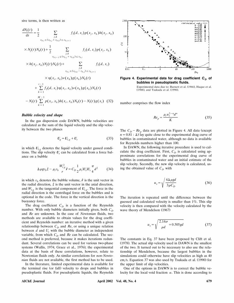
Figure 4. Experimental data for drag coefficient C ofDbubbles in pseudoplastic fluids.

Ž .Experimental data due to: Barnett et al. 1966 , Haque et al.Ž . Ž .1988 , and Tsukada et al. 1990 .

number comprises the flow index

r u2yndnc s

Re s 35Ž .p K

ŽThe C y Re data are plotted in Figure 4. All data exceptD p.ns0.81 : D lay quite close to the experimental drag curve of

bubbles in contaminated water, although no data is availablefor Reynolds numbers higher than 100.

In DAWN, the following iterative procedure is used to cal-culate the drag coefficient. First, C is calculated using ap-Dproximate correlations for the experimental drag curve ofbubbles in contaminated water and an initial estimate of theslip velocity. Secondly, the new slip velocity is calculated, us-ing the obtained value of C withD

4D r gdu s 36Ž .s ( 3rCD

The iteration is repeated until the difference between theguessed and calculated velocity is smaller than 1%. This slipvelocity is then compared with the velocity calculated by the

Ž .wave theory of Mendelson 1967

2.14su s q0.505gd 37Ž .s ( r d

The constants in Eq. 37 have been proposed by Clift et al.Ž .1978 . The actual slip velocity used in DAWN is the smallestof the two. It turned out to be necessary to also use the rela-tionship of Mendelson, because the largest bubbles in thesimulations could otherwise have slip velocities as high as 40

Ž .cmrs. Equation 37 was also used by Tsukada et al. 1990 forthe upper limit of slip velocities.

One of the options in DAWN is to correct the bubble ve-locity for the local void fraction a . This is done according to


Ž .Richardson and Zaki 1954

us qy1s 1y a 38Ž . Ž .u`

in which q is a function of the Reynolds number Re .pBubble Shapes. Important for the mass transfer}and in-

directly for C }is an accurate description of the surface areaDof a bubble. At low Reynolds and Eotvos numbers, interfacial¨ ¨tension and viscous forces are much more important than in-ertia forces, and the bubble has a spherical shape. At higherReynolds and Eotvos numbers, the bubbles are more ellip-¨ ¨

Ž . Ž .soidal with varying width a over height b ratio. The Eotvos¨ ¨number is defined as

g r d2e

Eos 39Ž .s

in which d is the diameter of a volume-equivalent sphere.eŽThe transition sphericalrellipsoidal see Figure 2.5 in Clift et

Ž ..al. 1978 is approximated by

w xlog Res1.205 ?exp y1.631 log Eo 40Ž .

The width to height ratio arb of an ellipse is calculated fromŽ .a plot presented by Harmathy 1960 . No special treatment

was introduced for spherical cap bubbles that will occur ifEo)40.

Mass transferThe mass-transfer coefficient k is calculated on the basisl

Ž .of the surface renewal concept of Kawase et al. 1987 . ThisŽ .concept is based on Higbie’s penetration theory Higbie, 1935Ž .and the surface renewal model of Danckwerts 1951 . In the

model, turbulence brings elements of bulk fluid up to thefree surface of a bubble, where unsteady mass transfer occursfor a time t , after which the element returns to the bulk ande

Ž .is replaced by another. k is then given by Higbie, 1935l

2 DDk s 41Ž .l (' tp e

The exposure time t is further modeled according to theeperiodic transitional sublayer model of Pinczewski and Side-

Ž . Žman 1974 . For power-law fluids, t is written as Kawasee.and Ulbrecht, 1983

1rnKrrŽ .q2t sT 42Ž .e 2rnn 0

in which Tq is a dimensionless bursting time period, and n 0Ž .is a friction velocity, given by Metkin and Sokolov 1982 as

Ž .1r2 1q nKnr2Ž1qn.n s2e 43Ž .0 ž /r

Substitution of Eqs. 42 and 43 into Eq. 41 yields

Ž .y1r2 1q n4 1 K1rn 1r2 1r2Ž1qn.k s 2 DD e 44Ž .l q ž /' T rp

where the factor 4 is included to account for the reducedexposure time at a free surface compared to a rigid surface,

q Žand the value of T is taken as 15.0 Kawase and Ulbrecht,.1983 . For Newtonian fluids, Eq. 44 reduces to

1r4y1r2k s3.01Sc en 45Ž . Ž .l

Ž .which was also used by Bakker and van den Akker 1994 intheir gas dispersion model GHOST!.

The local volumetric mass-transfer coefficient k a is calcu-llated when the surface area a of each bubble in a grid cell isbknown. In the case of ellipsoidal bubbles, the surface area isgiven by

2 2'ln arbq a rb y1b ž /2a s2p a 1q 46Ž .b 2 2a 'a rb y1

The summation of all the bubbles in each class then gives thelocal k al

M

k as k N a 47Ž .Ýl l i b , iis1

Integration of the local values of k a over the entire vessellgives the overall mass-transfer coefficient. In the output ofDAWN, both the overall value of k a and the local valueslare reported. This makes it possible to identify the regionswhere the highest mass-transfer rates occur.

Experimental SetupGlobal and local measurements of the gas fraction in a

stirred vessel have been performed to validate the predic-tions by the PBE model. The diameter T of the baffled ves-sel was 0.441 m, a six-blade Rushton type impeller was used

Ž .with diameter Ds0.147 m Figure 5 . The working fluid wasŽ .a 0.075 wt. % solution of Xanthan gum trade name Keltrol .

Its rheological behavior could well be described with the fol-lowing power-law parameters: K s0.0367 kg s2ynrm and ns0.65. The solution had a surface tension of s s0.0672 Nrm.

A ring sparger was placed midway between the flat vesselbottom and the impeller disc. The diameter of the spargerwas the same as the impeller disc diameter. In all cases, airwas used as the disperse phase. In the experiments, a gas-flowrate of Q s0.85 Lrs was used. The impeller speed was Nsg5.0 revrs, giving a power input of P s0.29 Wrkg. With thesegexperimental conditions, the gas was completely dispersed.

The power drawn was calculated from measuring the rota-tional speed of the impeller and the torque exerted by theimpeller. The overall gas holdup was visually determined byreading the liquid level. Local measurements of the gas frac-

Žtion were determined with an optical fiber probe Venneker,.1999 .


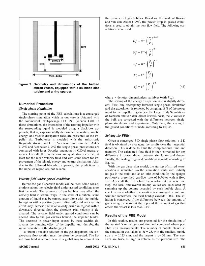
Figure 5. Geometry and dimensions of the baffledstirred vessel, equipped with a six-blade discturbine and a ring sparger.

Numerical ProcedureSingle-phase simulation

The starting point of the PBE calculations is a convergedsingle-phase simulation which in our case is obtained with

Ž .the commercial CFD-package FLUENT version 4.40 . Inthese simulations, the interaction of the rotating impeller withthe surrounding liquid is modeled using a black-box ap-proach, that is, experimentally determined velocities, kineticenergy, and viscous dissipation rates are presented at the im-peller tip. Turbulence is modeled with the anisotropicReynolds stress model. In Venneker and van den AkkerŽ . Ž .1997 and Venneker 1999 the single-phase predictions are

Ž .compared with laser Doppler anemometry LDA measure-ments. Overall, the predictions are qualitatively correct, atleast for the mean velocity field and with some room for im-provement of the kinetic energy and energy dissipation. Also,due to the followed black-box approach, the predictions inthe impeller region are not reliable.

Velocity field under gassed conditionsBefore the gas dispersion model can be used, some consid-

erations about the velocity field under gassed conditions mustfirst be made. The presence of gas bubbles may affect thevelocity field in several ways. In the wake of a bubble, someamount of liquid may be carried away along with the bubble.

Ž .In regions with a positive upward directed axial velocity thiseffect may increase the axial velocity, while in regions with adownward directed flow, the absolute axial velocity is de-creased. The velocity field under gassed conditions can bealtered also by the gas cavities behind the impeller blades.The decrease in power input caused by these cavities de-creases the pumping effect of the impeller and, thereby, theradial velocities in the discharge jet.

To obtain a reliable solution of the gas dispersion, the sin-gle-phase flow solution must therefore be corrected. The liq-uid flow field is altered here in a global way to account for

the presence of gas bubbles. Based on the work of RousarˇŽ .and van den Akker 1994 , the power drop in gassed condi-

tions is used to obtain the new flow field. The following cor-relations were used

0.65PgU UU sU ?g ž /P

0.4PgU UV sV ?g ž /P

0.65PgU UW sW ?g ž /P

PgU Uk s k ?g ž /P

2r3PgU Ue se ? 48Ž .g ž /P

Ž .where ) denotes dimensionless variables with V .tipThe scaling of the energy dissipation rate is slightly differ-

ent. First, any discrepancy between single-phase simulationand the experiment is removed by assigning 18% of the power

Žinput to the impeller region see the Large Eddy SimulationsŽ ..of Derksen and van den Akker 1998 . Next, the e values in

the bulk are corrected with the difference between single-phase simulation and experiment. Only then, the scaling tothe gassed conditions is made according to Eq. 48.

Sol©ing the PBEsGiven a converged 3-D single-phase flow solution, a 2-D

field is obtained by averaging the results over the tangentialdirection. This is done to limit the computational time andmemory. The calculated flow field is then corrected for anydifference in power drawn between simulation and theory.Finally, the scaling to gassed conditions is made according toEq. 48.

With the gas dispersion model, the startup of stirred vesselaeration is simulated. So the simulation starts with initially

Žno gas in the tank, and as an inlet condition at the sparger.position a prescribed gas-flow rate of bubbles with a fixed

size. After all the PBEs have been solved at the new timestep, the local and overall holdup values are calculated bysumming up the volume occupied by each bubble class. Acheck is made whether the solution is converged or not, andwhether somewhere the local holdup exceeds 100%. The so-lution is converged if the difference between the amount ofgas leaving the vessel at the top and the amount of gas thatenters the vessel is less than 0.1%.

Results of the PBE ModelIn this section, results are presented for the simulation of

the aerated Xanthan gum solution and compared where pos-sible with measurements. The number of bubble classes inthe simulation was taken as Ms25, with the smallest bubblesize d s0.125 mm, and the largest d s32 mm. The next1 25sizes are twice as large in volume as the previous size. The


Figure 6. PBE simulation results of 0.075% Keltrol.Ž . w x Ž .a Local gas fraction % in experiment; b predicted local

Ž . w x Ž .gas fraction; c predicted Sauter mean diameter m ; dw xpredicted mass transfer coefficient 1rs . Overall holdup ex-

periment: 3.6%"0.2; simulation: 3.08%. Overall db s 5.1932mm; Overall k as 0.0147 1rs.l

limits were determined by examining the bubble-size distri-bution in each computational cell and making sure that theamount of bubbles in the first and last class are practicallyzero. Finally, a time step of 0.01 s was used.

In Figures 6a and 6b, contour plots of the experimentallyand computationally determined local holdup values areshown. The measurements were performed at the intersec-tion of the drawn lines. The red areas in the figure denoteregions with gas fractions higher than 10%.

This figure clearly shows the potential strength of CFD ingeneral and of DAWN in particular; the internal distributionof gas inside a stirred vessel can now be calculated and iswith this first attempt using population balance equationsquite comparable with experiments. The model is capable ofpredicting the essential features of this particular flow regime:high gas fractions above the sparger and in the impeller out-flow; the concentration of gas in the upper part of the vessel;the accumulation of gas in the lower part of the vessel nearthe vessel wall; and the absence of gas beneath the sparger.

The reason why the two contour plots in Figure 6 are notidentical can be contributed to more than one fact. First, thesimulations are for an averaged 2-D field, whereas the mea-surements were performed in the plane between the baffles.Second, the errors in the gas fraction are to a large extentcaused by errors in the calculated single-phase flow field andthe subsequent scaling. With the solution strategy of DAWN,

Ž .improvements in the scaling of single-phase flow field areeasily extended to improvements in the gas fraction field.Also, in the formulation of DAWN, there is room for im-provement. Eventually, a two-way coupling between the liq-uid and the gas is necessary. At present however, the theoryon multiphase flow modeling is far from that point.

To perceive which future improvements are necessary, thesimulation is now analyzed in more detail. The experimentshows a clear meandering of the gas fraction field in the up-per part of the vessel. This meandering is caused by a smallliquid recirculation loop near the wall in the top of the ves-sel. This effect can also be seen in the drawing of the bulkflow patterns in an aerated stirred vessel of Nienow et al.Ž .1977 . The meandering is absent in the simulation, which isnot surprising because the secondary recirculation loop is alsonot present in the single-phase calculation. Clearly, a sub-stantial change in flow direction due to the presence of gascannot be predicted with this model.

ŽA striking fact are the higher gas fractions compared to.experiments in the bulk of the vessel. This can also be seen

in Figure 7, where a-profiles are shown for different heights.The overall holdup in the simulation was, however, lower thanobtained experimentally. The most plausible reason for thiscontradiction is the fact that not all bubbles were detected bythe glass fiber probe. Bubbles smaller than 1 mm are notpierced at all by the probe, while larger bubbles are not de-tected when their approach direction is not in line with theprobe tip.

Bubble Size and Mass-Transfer Predictions. As a final re-sult, contour plots of the local Sauter mean bubble diameterdb and the local mass-transfer coefficient k a are pre-32 l

Ž .sented see Figures 6c and d . In Figure 6c, it can be seenthat the smallest bubbles are localized in the lower part ofthe vessel, and not as one would expect, in the impeller re-gion. This is caused for the following reason. Small bubblesare formed in the impeller region where turbulence intensityis highest. In that region, not all bubbles are broken; as aconsequence, the minimum local value of db is not found32in the impeller outflow. At the height where the impeller out-flow reaches the vessel wall, the flow is divided into two cir-culation loops. The largest bubbly are mainly carried awaywith the upper loop, while small bubbles can be found ineither loop. In the circulation loops, turbulence intensity islow. With increasing height, db increases because of coales-32cence. This occurs in both loops, which explains the relativelyhigh bubble sizes in the lower corner of the vessel near thewall. From this latter region, only the smallest bubbles aretaken away towards the impeller, while the larger bubbleshave a sufficiently high slip velocity to escape and rise alongthe vessel wall. As a consequence, the region with the lowestdb is found in the lower corner near the symmetry axis,32which is a region with low gas fraction.

Bubble-size distributions in four characteristic positions inŽ .the vessel see Figure 6c are shown in Figure 8. Comparing


Figure 7. Measurements and predictions of the localgas fraction at several heights in 0.075% Kel-trol.Experimental conditions: N s 5.0 revrs, Q s1.0 Lrs, P sg g0.275 Wrkg.

points A, close to the impeller tip, and B, close to the wall,we see at point B that more smaller bubbles are present andthe class with the maximum number of bubbles has shiftedfrom 17 to 16. The region with the highest fraction of small-est bubbles is found just above the vessel bottom, and pointC shows a typical bubble-size distribution. Finally, point Dshows the distribution in the quiescent region in the upperpart of the tank where large bubbles are formed by coales-cence.

The bubble-size histograms can serve as a third validationmethod, next to measurements of the overall and local valuesof the gas fraction, of the model. Experimentally determinedbubble-size distributions can, for example, be obtained by a

Ž .suction probe Greaves and Barigou, 1988 or photographi-Ž .cally Takahashi and Nienow, 1993 .

The ability of predicting local bubble-size distributions isthe major advantage of the PBE formulation over two-fluidmodeling. It offers the possibility of investigating the internal

Figure 8. Bubble-size distribution as predicted byDAWN at characteristic positions in the ves-sel.

gas-liquid structure and can be used to improve the mass-transfer process.

The contour plot of k a shows that mass transfer is farlfrom uniform throughout the vessel, although the flow regimeis completely dispersed. The highest values of k a are foundlbelow the impeller disc and in the outflow of the impeller. Itmust be noted that in reality the bubble sizes directly be-neath the impeller disc are not as small as predicted by themodel. The specific area a is thus overpredicted there, mean-ing that the majority of the mass transfer occurs in the im-peller outflow. Given this irregular distribution of k a, it islobvious why multiple impellers are used in practical situa-tions.

ConclusionsA model has been presented based on the use of popula-

tion balance equations to simulate the behavior of bubbleswith different sizes in a turbulently agitated vessel. The inter-action between liquid and gas was assumed to be 1.5 waycoupled, and the liquid flow field is obtained from a single-phase flow simulation. With the model, local values of gasholdup, bubble size, number densities, and mass-transfer co-efficients in an aerated stirred tank can be calculated. Themodel predictions concerning local gas holdup are compara-ble with experiments and are encouraging enough to con-clude that the use of population balance equations is apromising technique to study dispersed flows. The main ad-vantage of using PBEs is that bubble-bubble interactions areexplicitly taken into account. Hence, research on mass trans-fer in dispersed flows can be carried out more accurately thanwith models with only one bubble size. In future work, themethodology as discussed in this article will be applied to


3-D, transient simulations of stirred tanks to realistically pre-dict gas dispersion.

AcknowledgmentsThe authors thank Kim Vahl for improving the simulation proce-

dure. This work was supported by the Netherlands Foundation forŽ .Chemical Research SON with financial aid from the Netherlands

Ž .Technology Foundation STW .

Notationasheigh of ellipse, masradius of thinning disc, mastotal specific bubble area, my1

a ssurface area of bubble, m2b

AsHamaker constant, kg ?m2 ? sy2

bswidth of ellipse, mBsbirth function, my4 ? sy1

csrelative speed of a bubble, m ? sy1

dsbubble diameter, mdb sSauter mean bubble diameter, m32

d sdiameter of a volume-equivalent sphere, meDsdeath function, my4 ? sy1

DDsdiffusion coefficient, m2 ? sy1

esenergy of an eddy, kg ?m2 ? sy2

essurface energy, kg ?m2 ? sy2

Esthree-dimensional energy spectrum, m3? sy2

f , f sfraction1 2g sbreakage frequency, sy1

hseffective swept volume rate, m3? sy1

hsfilm thickness, mh scritical film thickness at rupture, mch sinitial film thickness, m0kskinetic energy of turbulence per unit of mass, m2 ? sy2

kswave number, my1

k smass-transfer coefficient, m ? sy1l

K sconsistency, kg ? sny 2 ?my1

l sKolmogorov length micro scale, mdm smass of an eddy, kgl

Msnumber of bubble classesnsnumber density probability, my4

n snumber density probability of eddies, my4l

nsflow indexNsimpeller rotational speed, sy1

Nsnumber density, my3

pscoalescence efficiencyp sbreakage efficiencybP spower draw impeller, W ?kgy1

Q sgas-flow rate, m3? sy1gr sbubble radius, mr sradial co-ordinate, m

R sequivalent bubble radius, meqtstime, stsdrainage time, s

t sexposure time, set sdrainage time for deformable fully mobile interfaces, smob

T stank diameter, mTqsdimensionless bursting time

usbubble velocity, m ? sy1

u scritical eddy velocity, m ? sy1c

u sgas velocity, m ? sy1g

u seddy velocity as function of wave number, m ? sy1k

u sliquid velocity under gassed conditions, m ? sy1l, gu sbubble slip velocity, m ? sy1

su seddy velocity as function of eddy size, m ? sy1

l

Usmean axial velocity, m ? sy1

®scharacteristic velocity, m ? sy1

V sapproach velocity between bubbles, m ? sy1

V smean radial velocity, m ? sy1

W smean tangential velocity, m ? sy1

xsbubble diameter, mzsheight co-ordinate, m

Greek lettersa sgas fractione sdissipation rate of turbulent kinetic energy, m2 ? sy3

hsdaughter probability distribution, my1

Ž .lseddy size s kr2p , mn snumber of bubbles formed by breakage

n sfriction velocity, m ? sy10

r sdensity of continuous phase, kg ?my3c

s ssurface tension, kg ? sy2

t seddy turnover time, sv seddy-bubble collision rate, my1 sy1

Subscriptsbsbubble related variableg sgassed condition

i, j, jsclass indexlseddy related variable

Dimensionless groupsC sdrag coefficient, 4D r gdr3ru2

d sEosEotvos number, g r d2rs¨ ¨ c e

Re sbubble Reynolds number, r u2y ndnrKb c sScsSchmidt number, nrDD

WesWeber number, r u2drsc

Literature CitedBakker, A., ‘‘Hydrodynamics of Stirred Gas-Liquid Dispersions,’’PhD

Ž .Thesis, Delft Univ. of Technology 1992 .Bakker, A., and H. E. A. van den Akker, ‘‘A Computational Model

for the Gas-Liquid Flow in Stirred Reactors,’’ Trans. Inst. Chem.Ž .Eng., 72, 594 1994 .

Barnett, S. M., A. E. Humphrey, and M. Litt, ‘‘Bubble Motion andŽ .Mass Transfer in Non-Newtonian Fluids,’’ AIChE J., 12, 253 1966 .

Batchelor, G. K., ‘‘Pressure Fluctuations in Isotropic Turbulence,’’Ž .Proc. Camb. Phil. Soc., 47, 359 1951 .

Chesters, A. K., ‘‘The Applicability of Dynamic-Similarity Criteria toIsothermal, Liquid-Gas, Two-Phase Flows without Mass Transfer,’’

Ž .Int. J. Multiphase Flow, 2, 191 1975 .Chesters, A. K., ‘‘The Modelling of Coalescence Processes in Fluid-

Liquid Dispersions: A Review of Current Understanding,’’ Trans.Ž .Inst. Chem. Eng., 69, 25 1991 .

Clift, R., J. R. Grace, and M. E. Weber, Bubbles, Drops and Particles,Ž .Academic Press 1978 .

Coulaloglou, C. A., and L. L. Tavlarides, ‘‘Description of InteractionProcesses in Agitated Liquid-Liquid Dispersions,’’ Chem. Eng. Sci.,

Ž .32, 1289 1977 .Danckwerts, P. V., ‘‘Significance of Liquid-Film Coefficients in Gas

Ž .Absorption,’’ Ind. Eng. Chem., 43, 1460 1951 .Derksen, J. J., and H. E. A. van den Akker, ‘‘Parallel Simulation of

Turbulent Fluid Flow in a Mixing Tank,’’ Lecture Notes in Com-puter Science}High-performance Computing and Networking, P.

Ž .Sloot, M. Bubak, and B. Hertzberger, eds., Vol. 1401, p. 96 1998 .Djebbar, R., M. Roustan, and A. Line, ‘‘Numerical Computation of

Turbulent Gas-Liquid Dispersions in Mechanically Agitated Ves-Ž .sels,’’ Trans. Inst. Chem. Eng., 74, 492 1996 .

Gosman, A. D., C. Lekakou, S. Politis, R. I. Issa, and M. K. Looney,‘‘Multidimensional Modelling of Turbulent Two-Phase Flows in

Ž .Stirred Vessels,’’ AIChE J., 38, 1946 1992 .Grace, J. R., T. Wairegi, and T. H. Nguyen, ‘‘Shapes and Velocities

of Single Drops and Bubbles Moving Freely Through ImmiscibleŽ .liquids,’’ Trans. Inst. Chem. Eng., 54, 167 1976 .

Greaves, M., and M. Barigou, ‘‘The Internal Structure of Gas-LiquidDispersions in a Stirred Reactor,’’ Eur. Conf. on Mixing, Pavia, Italy,

Ž .p. 313 May 24]26, 1988 .


Haque, M. W., K. D. P. Nigam, K. Viswanathan, and J. B. Joshi,‘‘Studies on Bubble Rise Velocity in Bubble Columns Employing

Ž .Non-Newtonian Solutions,’’ Chem. Eng. Commun., 73, 31 1988 .Harmathy, T. Z., ‘‘Velocity of Large Drops and Bubbles in Media of

Ž .Infinite or Restricted Extent,’’ AIChE J., 6, 281 1960 .Hesketh, R. P., A. W. Etchells, and T. W. F. Russell, ‘‘Experimental

Observations of Bubble Breakage in Turbulent Flow,’’ Ind. Eng.Ž .Chem. Res., 30, 835 1991 .

Higbie, R., ‘‘The Rate of Absorption of a Pure Gas into a Still Liq-uid During Short Periods of Exposure,’’ Trans. AIChE, 31, 365Ž .1935 .

( )Hinze, J. O., Turbulence second edition , McGraw-Hill, New YorkŽ .1975 .

Hulburt, H. M., and S. L. Katz, ‘‘Some Problems in Particle Technol-ogy. A Statistical Mechanical Formulation,’’ Chem. Eng. Sci., 19,

Ž .555 1964 .Ishii, M., Thermo-fluid Dynamic Theory of Two-Phase Flow, EyrollesŽ .1975 .

Issa, R. I., and A. D. Gosman, ‘‘The Computation of Three-Dimen-sional Turbulent Two-Phase Flows in Mixer Vessels,’’ 2nd Int. Conf.

Ž .Numerical Methods in Laminar and Turbulent Flow, p. 827 1981 .Jenne, M., and M. Reuss, ‘‘Fluid Dynamic Modelling and Simulation

of Gas-Liquid Flow in Baffled Stirred Tank Reactors,’’ Mixing IX.Recent Ad®ances in Mixing, J. Bertrand and J. Villermaux, eds., 201Ž .1997 .

Kawase, Y., B. Halard, and M. Moo-Young, ‘‘Theoretical Predictionof Volumetric Mass Transfer Coefficients in Bubble Columns forNewtonian and Non-Newtonian Fluids,’’ Chem. Eng. Sci., 42, 1609Ž .1987 .

Kawase, Y., and J. J. Ulbrecht, ‘‘Turbulent Heat and Mass Transferin Non-Newtonian Pipe-Flow: a Model Based on the Surface Re-

Ž .newal Concept,’’ Phys. Chem. Hydr., 4, 351 1983 .Kirkpatrick, R. D., and M. J. Lockett, ‘‘The Influence of Approach

Ž .Velocity on Bubble Coalescence,’’ Chem. Eng. Sci., 29, 2363 1974 .Kolmogorov, A. N., ‘‘Local Structure of Turbulence in Incompress-

ible Viscous Fluid for Very Large Reynolds Number,’’ Dokl. Akad.Ž .Nauk SSSR, 30, 229 1941 .

Kuboi, R., I. Komasawa, and T. Otake, ‘‘Behavior of Dispersed Par-Ž .ticles in Turbulent Liquid Flow,’’ J. Chem. Eng. Jap., 5, 349 1972 .

Lathouwers, D., and H. E. A. van den Akker, ‘‘A Numerical Methodfor the Solution of Two-Fluid Model Equations,’’ Numerical Meth-

Ž .ods for Multiphase Flow, FED, Vol. 236, p. 121 1996 .Levich, V. G., Physicochemical Hydrodynamics, Prentice-Hall, Engle-

Ž .wood Cliffs, NJ 1962 .Lewalle, J., L. L. Tavlarides, and V. Jairazbhoy, ‘‘Modeling of Tur-

bulent, Neutrally Buoyant Droplet Suspensions in Liquids,’’ Chem.Ž .Eng. Comm., 59, 15 1987 .

Luo, H., and H. F. Svendsen, ‘‘Theoretical Model for Drop and Bub-Ž .ble Breakup in Turbulent Dispersions,’’ AIChE J., 42, 1225 1996 .

Mendelson, H. D., ‘‘The Prediction of Bubble Terminal VelocitiesŽ .from Wave Theory,’’ AIChE J., 13, 250 1967 .

Metkin, V. P., and V. N. Sokolov, ‘‘Hydraulic Resistance to Flow ofGas-Liquid Mixtures Having Non-Newtonian Properties,’’ J. Appl.

Ž .Chem. USSR, 55, 558 1982 .Morud, K. E., and B. H. Hjertager, ‘‘LDA Measurements and CFD

Modelling of Gas-Liquid Flow in a Stirred Vessel,’’ Chem. Eng.Ž .Sci., 51, 233 1996 .

Nienow, A. W., D. J. Wisdom, and J. C. Middleton, ‘‘The Effect ofScale and Geometry on Flooding, Recirculation, and Power inGassed Stirred Vessels,’’ 2nd Eur. Conf. on Mixing, Cambridge,

Ž .U.K., 1 1977 .Ž .Pinczewski, W. V., and S. Sideman, ‘‘A Model for Mass Heat

Transfer in Turbulent Tube Flow. Moderate and High SchmidtŽ . Ž .Prandtl Numbers,’’ Chem. Eng. Sci., 29, 1969 1974 .

Prince, M. J., and H. W. Blanch, ‘‘Bubble Coalescence and Break-UpŽ .in Air-Sparged Bubble Columns,’’ AIChE J., 36, 1485 1990 .

Ramkrishna, D., ‘‘The Status of Population Balances,’’ Re®. in Chem.Ž .Eng., 3, 49 1985 .

Richardson, J. F., and W. F. Zaki, ‘‘Sedimentation and Fluidisation:Ž .I,’’ Trans. Inst. Chem. Engrs., 32, 35 1954 .

Ritchie, B. W., and A. H. Togby, ‘‘General Population Balance Mod-elling of Unpremixed Feedstream Chemical Reactors: a Review,’’

Ž .Chem. Eng. Comm., 2, 249 1978 .Rousar, I., and H. E. A. van den Akker, ‘‘LDA Measurements ofˇ

Liquid Velocities in Sparged Agitated Tanks with Single and Mul-tiple Rushton Turbines,’’ 8th Eur. Conf. on Mixing, Cambridge,

Ž .U.K., 89 Sept. 21]23, 1994 .Takahashi, K., and A. W. Nienow, ‘‘Bubble Sizes and Coalescence

Rates in an Aerated Vessel Agitated by a Rushton Turbine,’’ J.Ž .Chem. Eng. Jap., 26, 536 1993 .

Tennekes, H., and J. L. Lumley, A First Course in Turbulence, MITŽ .Press, Cambridge, MA 1972 .

Tsouris, C., and L. L. Tavlarides, ‘‘Breakage and Coalescence Mod-Ž .els for Drops in Turbulent Dispersions,’’ AIChE J., 40, 395 1994 .

Tsukada, T., H. Mikami, M. Hozawa, and N. Imaishi, ‘‘Theoreticaland Experimental Studies of the Deformation of Bubbles Movingin Quiescent Newtonian and Non-Newtonian Liquids,’’ J. Chem.

Ž .Eng. Jap., 23, 192 1990 .van Santen, H., D. Lathouwers, C. R. Kleijn, and H. E. A. van den

Akker, ‘‘Influence of Segregation on the Efficiency of Finite Vol-ume Methods for the Incompressible Navier-Stokes Equations,’’

Ž .Proc. of Fluid Eng. Di®. of ASME, Vol. 3, FED Vol. 238, 151 1996 .Venneker, B. C. H., ‘‘Turbulence Flow and Gas Dispersion in Stirred

Vessels with Pseudo-Plastic Liquids,’’ PhD Thesis, Delft UniversityŽ .of Technology 1999 .

Venneker, B. C. H., and H. E. A. van den Akker, ‘‘CFD Calculationsof the Turbulent Flow of Shear-Thinning Fluids in Agitated Tanks,’’Mixing IX. Recent Ad®ances in Mixing, J. Bertrand and J. Viller-

Ž .maux, eds., 179 1997 .Wallis, G. B., ‘‘The Terminal Speed of Single Drops or Bubbles in

Ž .an Infinite Medium,’’ Int. J. Multiphase Flow, 1, 491 1974 .Manuscript recei®ed Mar. 29, 2001, and re®ision recei®ed Oct. 1, 2001.


population balance modeling of aerated stirred vessels

Documents