popeye g-sand log responses and synthetic seismogram ties v 1 · · 2016-01-13popeye g-sand log...
TRANSCRIPT
Popeye G-SandLog Responses and Synthetic
Seismogram Tiesv 1.0
Tin-Wai LeeNovember 2002
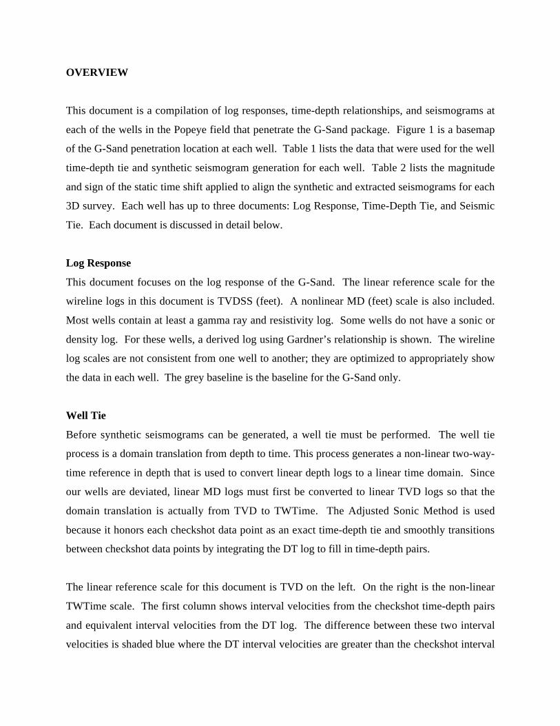
OVERVIEW
This document is a compilation of log responses, time-depth relationships, and seismograms at
each of the wells in the Popeye field that penetrate the G-Sand package. Figure 1 is a basemap
of the G-Sand penetration location at each well. Table 1 lists the data that were used for the well
time-depth tie and synthetic seismogram generation for each well. Table 2 lists the magnitude
and sign of the static time shift applied to align the synthetic and extracted seismograms for each
3D survey. Each well has up to three documents: Log Response, Time-Depth Tie, and Seismic
Tie. Each document is discussed in detail below.
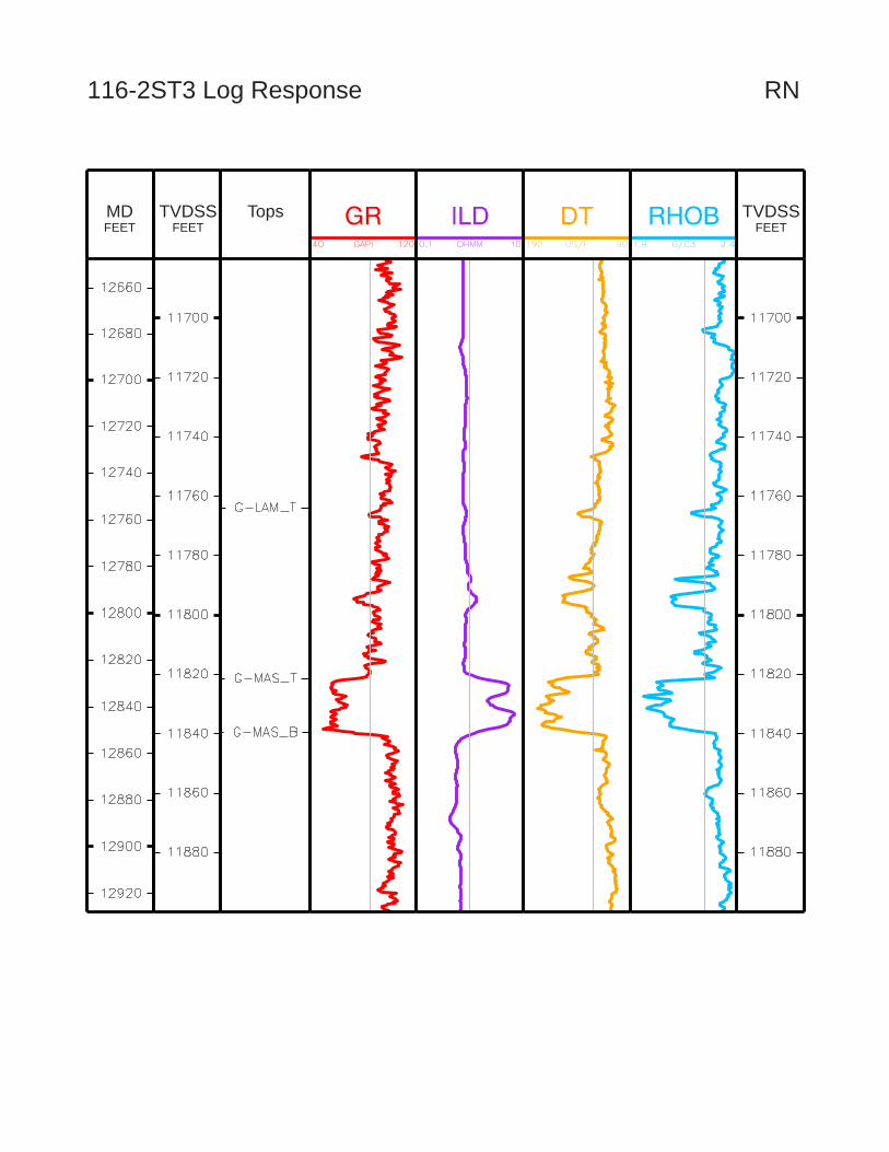
Log Response
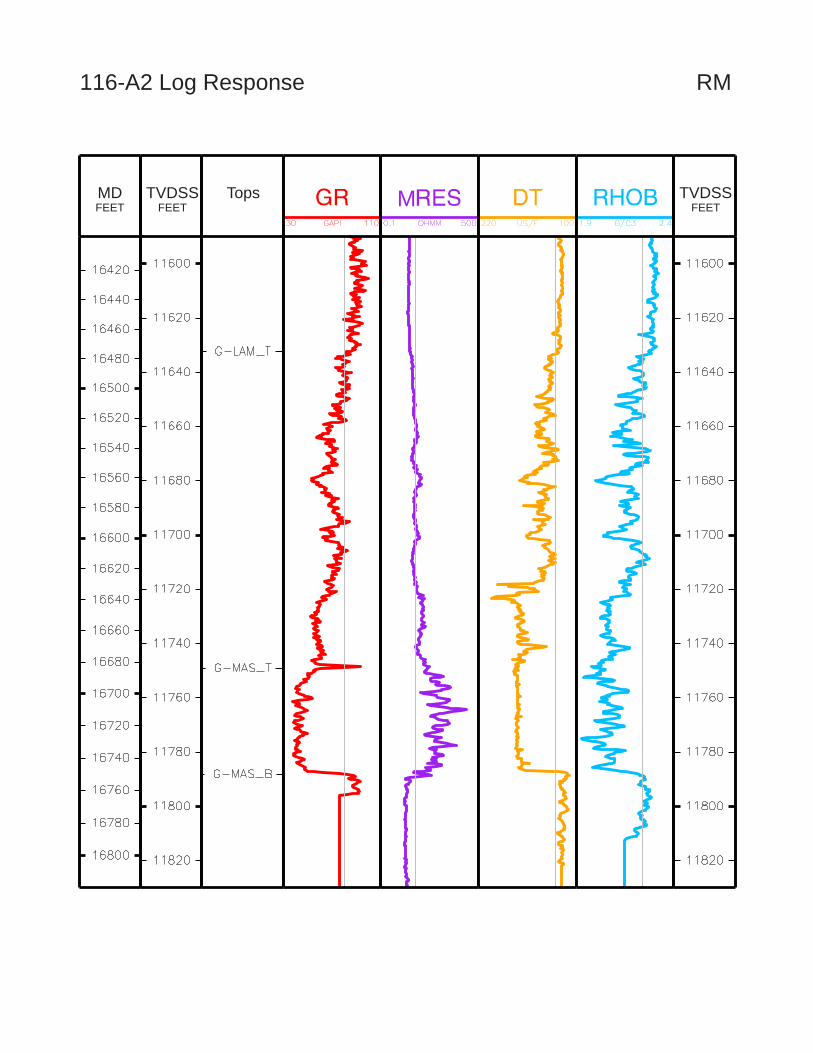
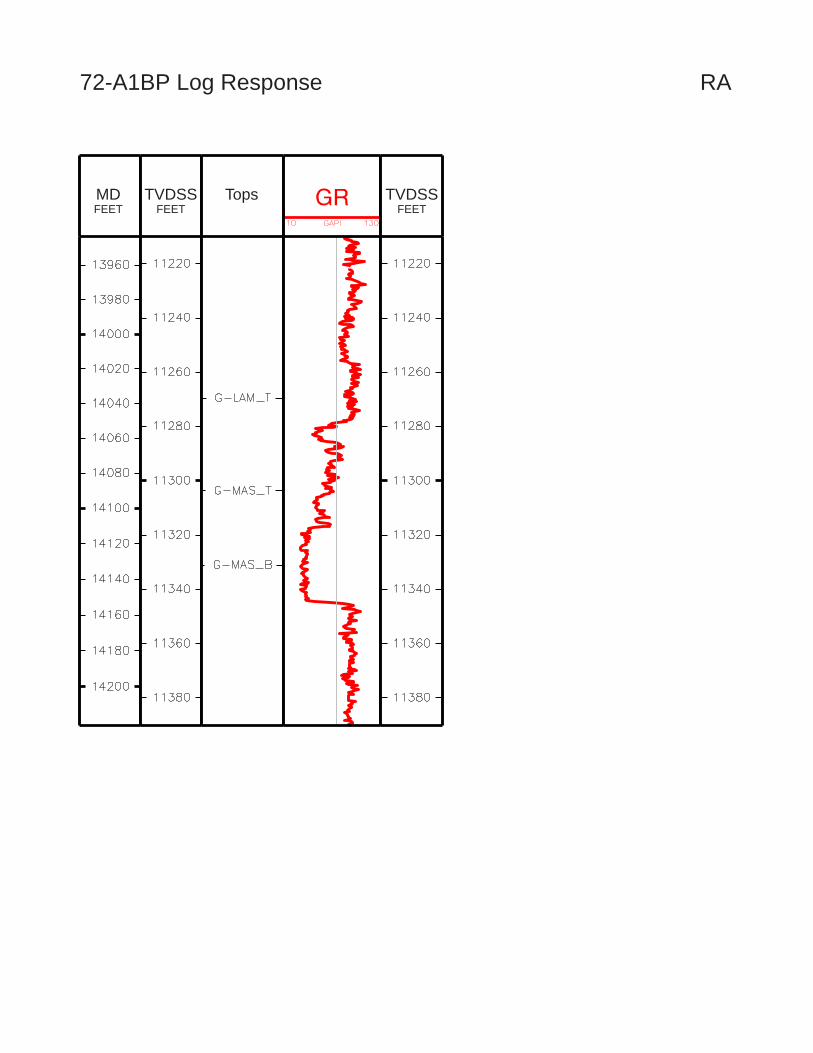
This document focuses on the log response of the G-Sand. The linear reference scale for the
wireline logs in this document is TVDSS (feet). A nonlinear MD (feet) scale is also included.
Most wells contain at least a gamma ray and resistivity log. Some wells do not have a sonic or
density log. For these wells, a derived log using Gardner’s relationship is shown. The wireline
log scales are not consistent from one well to another; they are optimized to appropriately show
the data in each well. The grey baseline is the baseline for the G-Sand only.
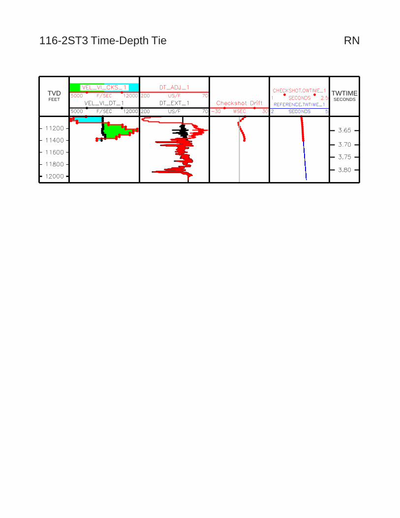
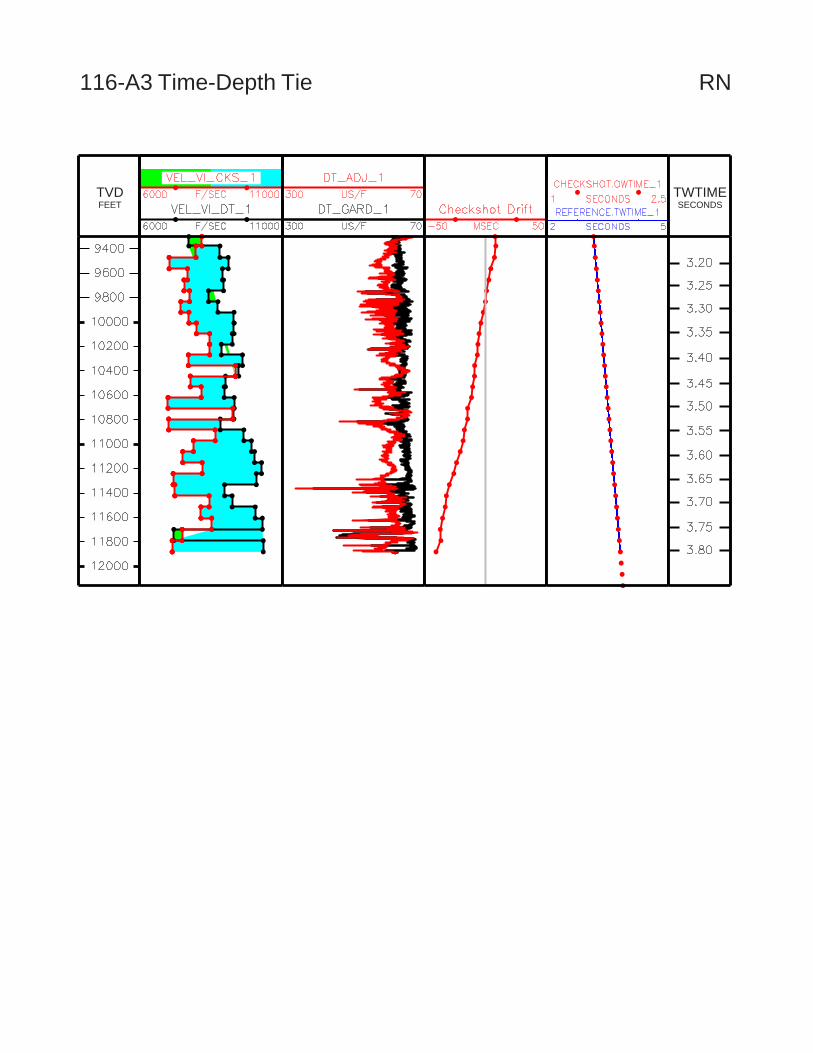
Well Tie
Before synthetic seismograms can be generated, a well tie must be performed. The well tie
process is a domain translation from depth to time. This process generates a non-linear two-way-
time reference in depth that is used to convert linear depth logs to a linear time domain. Since
our wells are deviated, linear MD logs must first be converted to linear TVD logs so that the
domain translation is actually from TVD to TWTime. The Adjusted Sonic Method is used
because it honors each checkshot data point as an exact time-depth tie and smoothly transitions
between checkshot data points by integrating the DT log to fill in time-depth pairs.
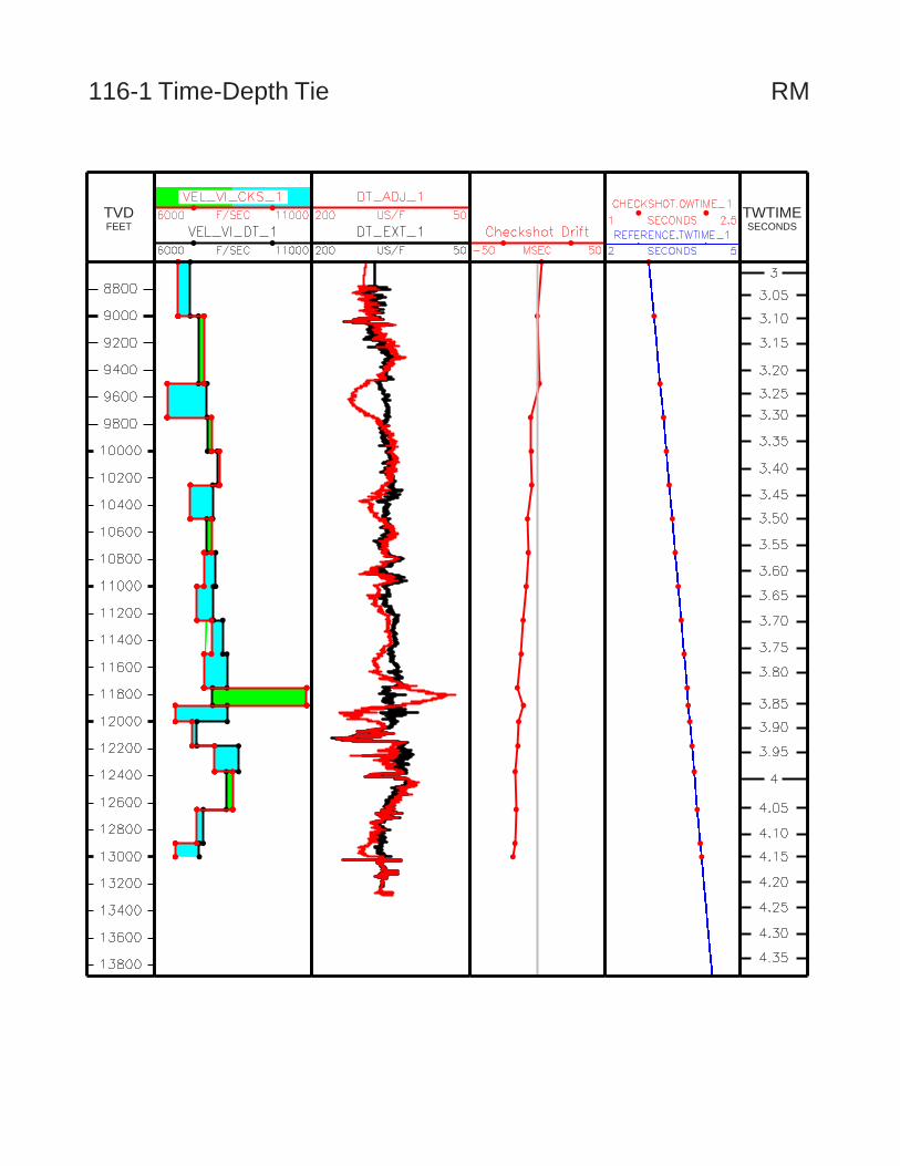
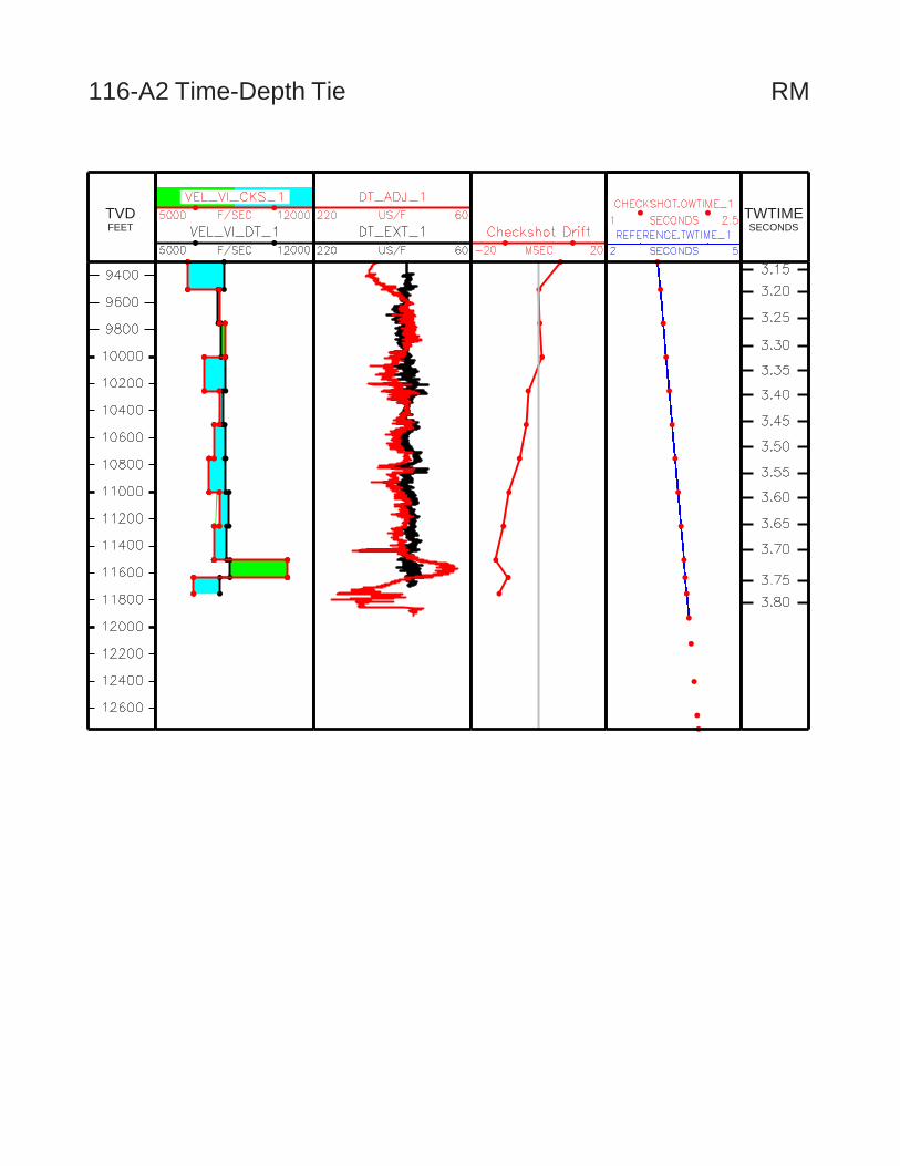
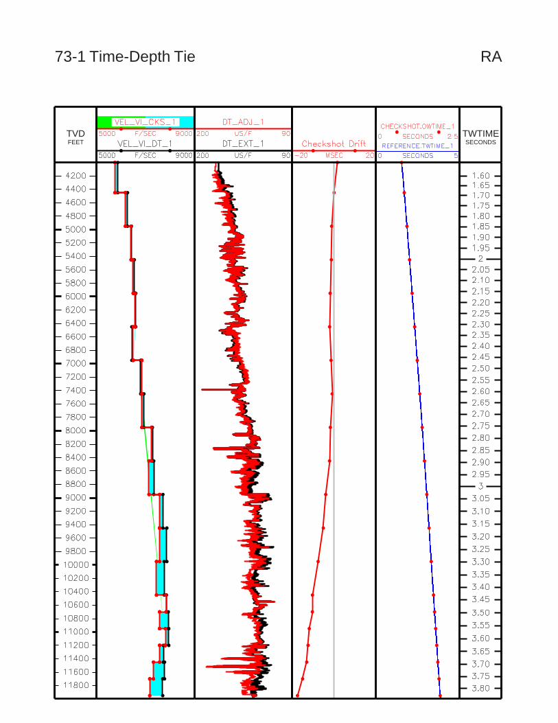
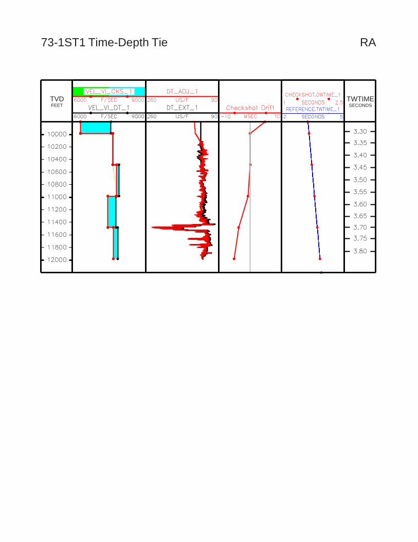
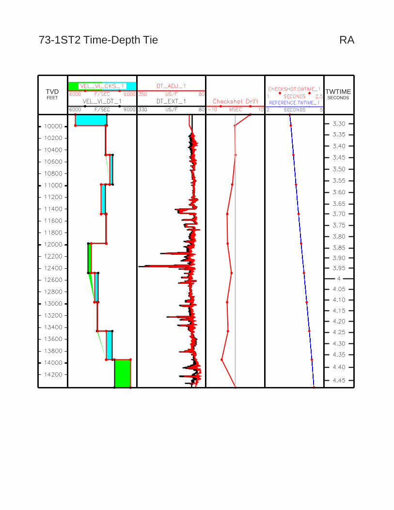
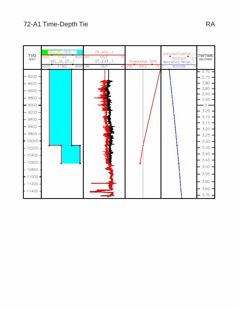
The linear reference scale for this document is TVD on the left. On the right is the non-linear
TWTime scale. The first column shows interval velocities from the checkshot time-depth pairs
and equivalent interval velocities from the DT log. The difference between these two interval
velocities is shaded blue where the DT interval velocities are greater than the checkshot interval
velocities. It is shaded green where the checkshot interval velocities are greater than the DT
interval velocities. The second column shows both the input DT log in black and the adjusted
DT log in red. The adjusted DT log is the reconciled DT log that incorporates the checkshot
drift. The middle column shows checkshot drift in ms. Checkshot drift is the difference in
TWTime between the integrated sonic and the checkshot survey. Checkshot drift is set to zero at
the first checkshot datapoint below the start of the DT and RHOB logs, and should smoothly
increase with depth. Any kinks may represent a bad checkshot data point or a true distinct
velocity due to lithology or overpressure. Checkshot surveys with closely spaced datapoints are
more likely to have kinks. The last column shows the resulting time-depth relationship with the
checkshot data points lying exactly on it.
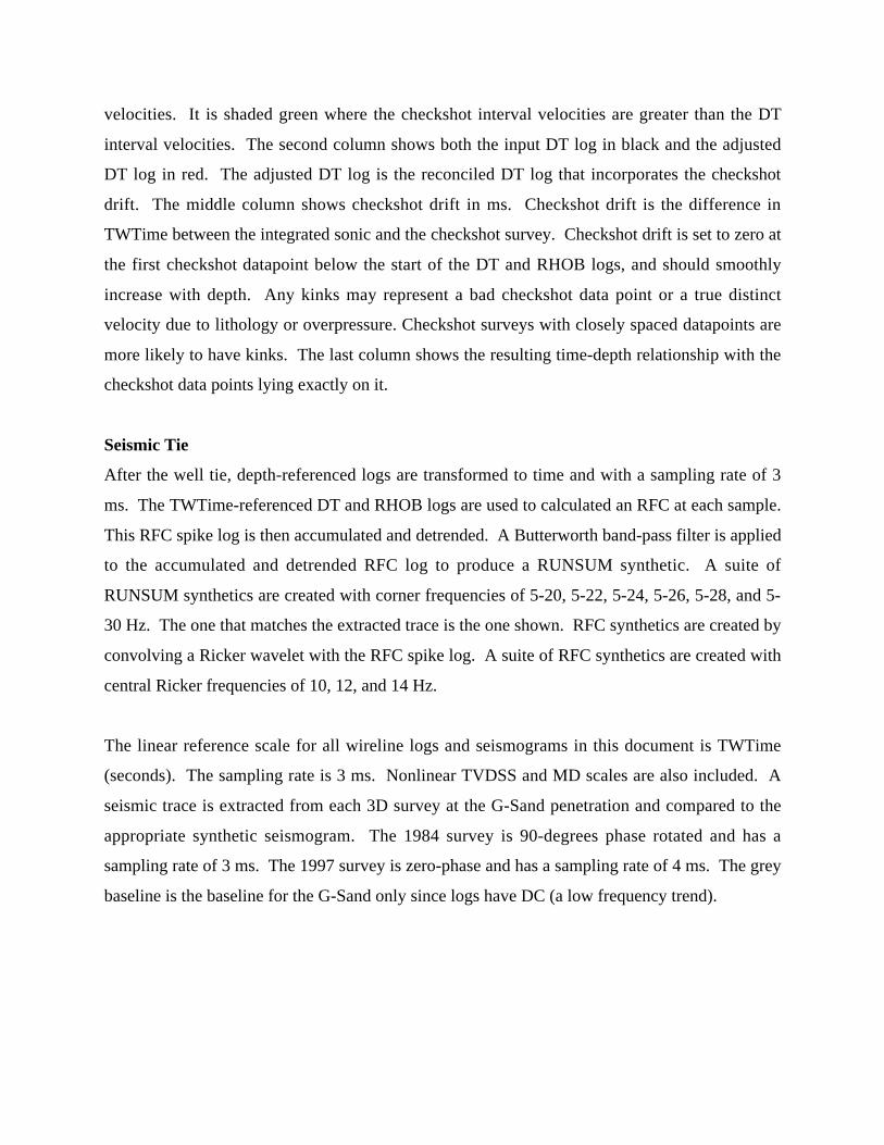
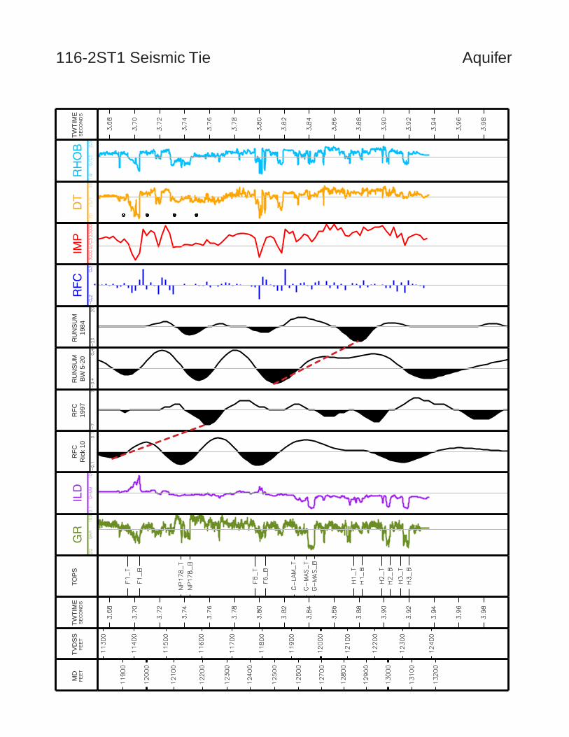
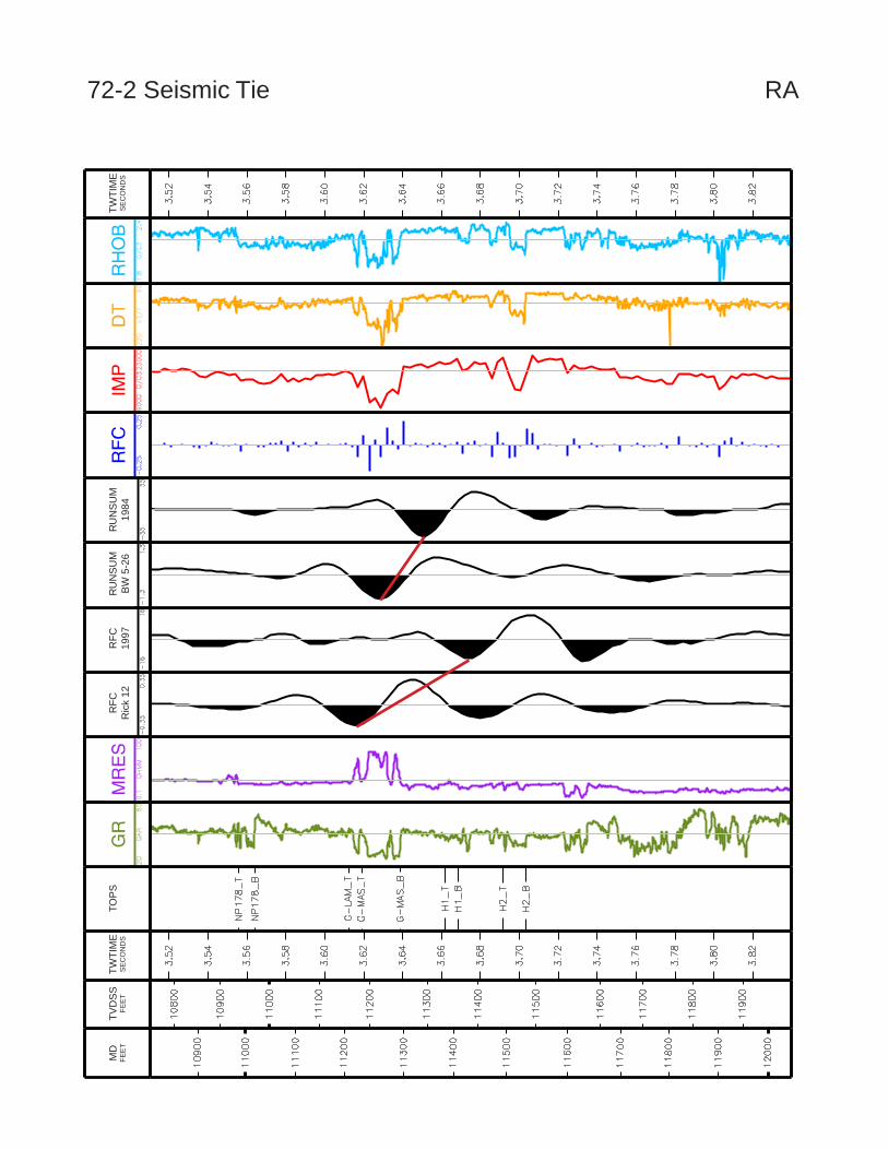
Seismic Tie
After the well tie, depth-referenced logs are transformed to time and with a sampling rate of 3
ms. The TWTime-referenced DT and RHOB logs are used to calculated an RFC at each sample.
This RFC spike log is then accumulated and detrended. A Butterworth band-pass filter is applied
to the accumulated and detrended RFC log to produce a RUNSUM synthetic. A suite of
RUNSUM synthetics are created with corner frequencies of 5-20, 5-22, 5-24, 5-26, 5-28, and 5-
30 Hz. The one that matches the extracted trace is the one shown. RFC synthetics are created by
convolving a Ricker wavelet with the RFC spike log. A suite of RFC synthetics are created with
central Ricker frequencies of 10, 12, and 14 Hz.
The linear reference scale for all wireline logs and seismograms in this document is TWTime
(seconds). The sampling rate is 3 ms. Nonlinear TVDSS and MD scales are also included. A
seismic trace is extracted from each 3D survey at the G-Sand penetration and compared to the
appropriate synthetic seismogram. The 1984 survey is 90-degrees phase rotated and has a
sampling rate of 3 ms. The 1997 survey is zero-phase and has a sampling rate of 4 ms. The grey
baseline is the baseline for the G-Sand only since logs have DC (a low frequency trend).

Well without seismic-tie
Well with seismic-tie
116-A2BP
116-A3
72-A1ST
72-A1BP72-A1
73-1
73-1ST1 73-1ST2
116-2 116-2ST1
116-2ST3
116-2ST2
72-272-1
116-1
116 117
72 73
116-A2
0 1 km
0 1 mi
Basemap
RM
RN
RA
RB
N

DATA USED
Table 1 summarizes the data used for the time-depth tie and synthetic seismogram creation.
Table 1: Data Used
A check indicates that the well uses its own data. If a well does not have its own checkshot
survey, an edited checkshot survey from a nearby well is used. This editing process assumes that
the geology is the same between the location of the checkshot survey and the location of the well
without a checkshot survey. It only compensates for the difference in KB and WD between the
two locations in both the depths and times so that interval velocities remain the same. If a well
does not have a DT or a RHOB log, then one is derived from the other using Gardner’s
relationship as follows:
Well Checkshot DT RHOB
116-1 � � �
116-2 � � �
116-2ST1 � � �
116-2ST2 � � �
116-2ST3 116-2ST2 � �
116-A2 116-1 � �
116-A2BP 116-1 � �
116-A3 116-2 Gardner �
72-1 -- -- --
72-2 � � �
72-A1 72-2 � �
72-A1BP -- -- --
72-A1ST -- -- --
73-1 � � �
73-1ST1 � � �
73-1ST2 73-1ST1 � Gardner

ρ = 0.23⋅ v0.25
RHOB = 0.23⋅ 106
DT
0.25
DT = 106
RHOB0.23
4
If a well does not have both DT and RHOB logs nor a checkshot survey, then neither a time-
depth tie nor a seismic tie is performed for the well. This is the case for wells 72-1, 72-A1PB,
and 72-A1ST.

SEISMOGRAM SHIFT
Table 2 summarizes the amount of static time shift in seconds that is necessary to align the
extracted seismogram of both surveys to the synthetic seismogram at each well. The amount of
shift is defined as:
Shift = TWTime (synthetic) – TWTime (extracted)
Therefore a negative shift indicates that the extracted trace was deeper than the synthetic trace
and a positive shift indicates that the extracted trace was shallower than the synthetic trace.
Table 2: Static Shift to Align Extracted and Synthetic Seismograms
The amount of shift is usually calculated on the time-depth pair of the trough minima that
represents the top of the G-Sand in zero-phase data and the middle of the G-Sand in RUNSUM
1997 1984Shift (s) Shift (s)
116-1 -0.048 -0.024
116-2 -0.046 -0.033
116-2ST1 -0.072 -0.066
116-2ST2 -0.082 -0.066
116-2ST3 -0.075 -0.066
116-A2 -0.116 -0.096
116-A2BP -0.125 -0.108
116-A3 -0.063 -0.054
72-1 -- --
72-2 -0.054 -0.021
72-A1 -0.056 -0.027
72-A1BP -- --
72-A1ST -- --
73-1 -0.039 0.003
73-1ST1 -0.078 -0.01873-1ST2 -0.084 -0.030
Well

data. Where it is difficult or impossible to identify the G-Sand trough minima, the amount of
shift is calculated on the time-depth pair of either the peak maxima below the G-Sand trough
minima or the trough minima of another sand. This was necessary for the wet well (116-2ST1),
the well with only 6 ft of G-Sand (73-1), and also 116-A2 and 116-A2BP.
Both RFC and RUNSUM synthetics were created with a sampling rate of 3 ms, which is the
same sampling rate as the 1984 dataset. Therefore the shift for the 1984 dataset is an integer
multiple of 3 ms. Since the sampling rate of the 1997 dataset is 4 ms, the shift is a multiple of 1
ms.

TVDSSFEET
TVDSSFEET
MDFEET
Tops
116-2 Log Response RN

TWTIMESECONDS
TVDFEET
116-2 Time-Depth Tie RN
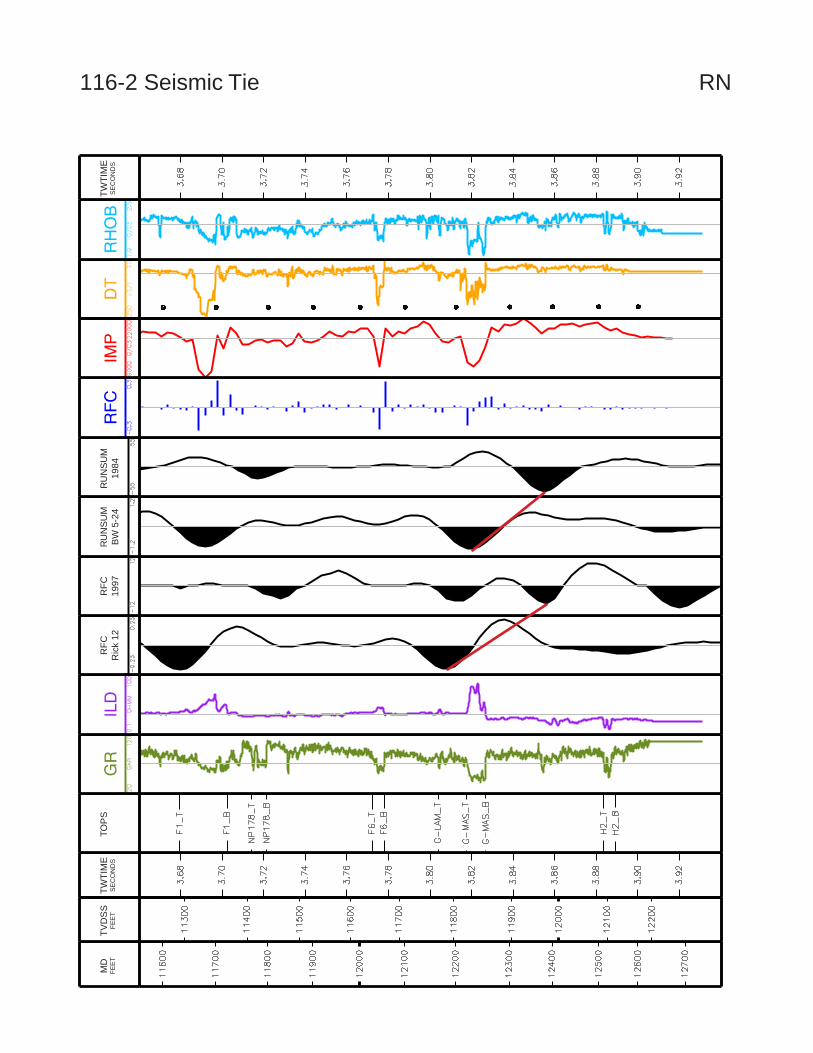
116-2 Seismic Tie T
VD
SS
FE
ET
TOP
SR
FC
Ric
k 12
RF
C19
97R
UN
SU
MB
W 5
-24
RU
NS
UM
1984
TW
TIM
ES
EC
ON
DS
TW
TIM
ES
EC
ON
DS
MD
FE
ET
RN

TVDSSFEET
TVDSSFEET
MDFEET
Tops
116-2ST2 Log Response RN

TWTIMESECONDS
TVDFEET
116-2ST2 Time-Depth Tie RN

TV
DS
SF
EE
TTO
PS
RF
CR
ick
12R
FC
1997
RU
NS
UM
BW
5-2
4R
UN
SU
M19
84T
WT
IME
SE
CO
ND
ST
WT
IME
SE
CO
ND
SM
DF
EE
T
116-2ST2 Seismic Tie RN
TVDSSFEET
TVDSSFEET
MDFEET
Tops
116-2ST3 Log Response RN
TWTIMESECONDS
TVDFEET
116-2ST3 Time-Depth Tie RN

TV
DS
SF
EE
TTO
PS
RF
C19
97R
UN
SU
MB
W 5
-24
RU
NS
UM
1984
TW
TIM
ES
EC
ON
DS
TW
TIM
ES
EC
ON
DS
MD
FE
ET
116-2ST3 Seismic Tie RNR
FC
Ric
k 12

116-A3 Log Response
TVDSSFEET
TVDSSFEET
MDFEET
Tops
RN
The sonic log is derived from the density log using Gardner's relationship.
TWTIMESECONDS
TVDFEET
116-A3 Time-Depth Tie RN

TV
DS
SF
EE
TTO
PS
RF
CR
ick
12R
FC
1997
RU
NS
UM
BW
5-2
0R
UN
SU
M19
84T
WT
IME
SE
CO
ND
ST
WT
IME
SE
CO
ND
SM
DF
EE
T
RN116-A3 Seismic Tie

TVDSSFEET
TVDSSFEET
MDFEET
Tops
116-2ST1 Log Response Aquifer

TWTIMESECONDS
TVDFEET
116-2 ST1 Time-Depth Tie Aquifer
TV
DS
SF
EE
TTO
PS
RF
CR
ick
10R
FC
1997
RU
NS
UM
BW
5-2
0R
UN
SU
M19
84T
WT
IME
SE
CO
ND
ST
WT
IME
SE
CO
ND
SM
DF
EE
T
116-2ST1 Seismic Tie Aquifer

TVDSSFEET
TVDSSFEET
MDFEET
Tops
116-1 Log Response RM
TWTIMESECONDS
TVDFEET
116-1 Time-Depth Tie RM

TV
DS
SF
EE
TTO
PS
RF
CR
ick
10R
FC
1997
RU
NS
UM
BW
5-2
8R
UN
SU
M19
84T
WT
IME
SE
CO
ND
ST
WT
IME
SE
CO
ND
SM
DF
EE
T
116-1 Seismic Tie RM
TVDSSFEET
TVDSSFEET
MDFEET
Tops
116-A2 Log Response
M
RM
TWTIMESECONDS
TVDFEET
116-A2 Time-Depth Tie RM

TV
DS
SF
EE
TTO
PS
RF
C19
97R
UN
SU
MB
W 5
-28
RU
NS
UM
1984
TW
TIM
ES
EC
ON
DS
TW
TIM
ES
EC
ON
DS
MD
FE
ET
RM116-A2 Seismic Tie R
FC
Ric
k 14

TVDSSFEET
TVDSSFEET
MDFEET
Tops
116-A2BP Log Response RM

TWTIMESECONDS
TVDFEET
116-A2BP Time-Depth Tie RM

TV
DS
SF
EE
TTO
PS
RF
CR
ick
12R
FC
1997
RU
NS
UM
BW
5-2
4R
UN
SU
M19
84T
WT
IME
SE
CO
ND
ST
WT
IME
SE
CO
ND
SM
DF
EE
T
116-A2BP Seismic Tie RM

TVDSSFEET
TVDSSFEET
MDFEET
Tops
73-1 Log Response RA
TWTIMESECONDS
TVDFEET
73-1 Time-Depth Tie RA

TV
DS
SF
EE
TTO
PS
RF
CR
ick
10R
FC
1997
RU
NS
UM
BW
5-2
8R
UN
SU
M19
84T
WT
IME
SE
CO
ND
ST
WT
IME
SE
CO
ND
SM
DF
EE
T
RA73-1 Seismic Tie

73-1ST1 Log Response
TVDSSFEET
TVDSSFEET
MDFEET
Tops
RA
TWTIMESECONDS
TVDFEET
73-1ST1 Time-Depth Tie RA

TV
DS
SF
EE
TTO
PS
RF
CR
ick
12R
FC
1997
RU
NS
UM
BW
5-3
0R
UN
SU
M19
84T
WT
IME
SE
CO
ND
ST
WT
IME
SE
CO
ND
SM
DF
EE
T
RA73-1ST1 Seismic Tie

TVDSSFEET
TVDSSFEET
MDFEET
Tops
73-1ST2 Log Response RA
The density log is derived from the sonic log using Gardner's relationship.
TWTIMESECONDS
TVDFEET
73-1ST2 Time-Depth Tie RA

TV
DS
SF
EE
TTO
PS
RF
CR
ick
12R
FC
1997
RU
NS
UM
BW
5-2
8R
UN
SU
M19
84T
WT
IME
SE
CO
ND
ST
WT
IME
SE
CO
ND
SM
DF
EE
T
RA73-1ST2 Seismic Tie

72-A1 Log Response
TVDSSFEET
TVDSSFEET
MDFEET
Tops
RA
TWTIMESECONDS
TVDFEET
72-A1 Time-Depth Tie RA

TV
DS
SF
EE
TTO
PS
RF
CR
ick
12R
FC
1997
RU
NS
UM
BW
5-2
6R
UN
SU
M19
84T
WT
IME
SE
CO
ND
ST
WT
IME
SE
CO
ND
SM
DF
EE
T
RA72-A1 Seismic Tie

72-A1ST Log Response
TVDSSFEET
TVDSSFEET
MDFEET
Tops
RA
72-A1BP Log Response
TVDSSFEET
TVDSSFEET
MDFEET
Tops
RA
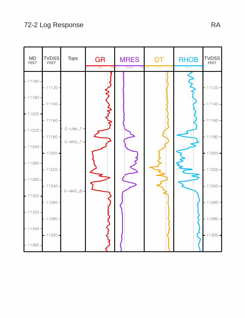
72-2 Log Response
TVDSSFEET
TVDSSFEET
MDFEET
Tops
RA

TWTIMESECONDS
TVDFEET
72-2 Time-Depth Tie RA
TV
DS
SF
EE
TTO
PS
RF
CR
ick
12R
FC
1997
RU
NS
UM
BW
5-2
6R
UN
SU
M19
84T
WT
IME
SE
CO
ND
ST
WT
IME
SE
CO
ND
SM
DF
EE
T
RA72-2 Seismic Tie