ponza 05 june 2008 status report on analysis f. ambrosino t. capussela f. perfetto status...
TRANSCRIPT

Ponza 05 June 2008
Status report on analysis
F. Ambrosino T. Capussela F. Perfetto
Status report on analysisFrascati 29 September 2008

Outline Now Future Conclusions
Ponza 05 June 2008
Outline
Where we stand now:
Improved the selection procedure Tested the fit procedure Semplified the analysis Which are the future plans:
Understand the slope in the wrong pairing (w.p.) Select the approach in which to give the result Finally to publish!!!!
Frascati 29 September 2008

OLD approach:
7 and only 7 pnc with 21° < < 159° and E > 10 MeV > 18° Kin Fit with no mass constraint P(2) > 0.01 320 MeV < Erad < 400 MeV AFTER PHOTON’S PAIRINGKinematic Fit with and mass
constraints (on DATA M= 547.822
MeV/c2 )
NEW approach:
7 and only 7 pnc with 21° < < 159° and E > 10 MeV > 18° Kin Fit with mass constraint
(on DATA M= 547.874 MeV/c2 ) P(2) > 0.01 320 MeV < Erad < 400 MeV AFTER PHOTON’S PAIRINGKinematic Fit with mass constraint
Frascati 29 September 2008
Outline Now Future Conclusions
Sample selection

Outline Now Future Conclusions
Ponza 05 June 2008
Zgen in acceptance
Frascati 29 September 2008
After kinematic fit After P(2) > 0.01
After EVCL
After > 18°
After E > 10 MeV
After 320 MeV < Erad < 400 MeV

Outline Now Future Conclusions
Ponza 05 June 2008
Effect on purity and efficiency new approach
Frascati 29 September 2008
> 18°
> 15°
> 12°
> 9° > 6°
PUR % 82.2 82.1 81.9 81.7 81.4
% 12.4 8.2 6.8 4.9 4.7
PUR % 89.4 89.3 89.2 89 88.9
% 15.8 13.1 11.1 9.1 8.9
PUR % 95.1 95.0 94.9 94.8 94.7
% 22 19.2 16.8 14.6 13.6
PUR % 97.1 97.0 96.9 96.9 96.8
% 28 26 23 20.4 19
PUR % 99 98.97 98.95 98.88 98.8
% 27 21.4 20.7 18 16.6
Low
Med I
Med II
Med III
High
Outline Now Future Conclusions
Ponza 05 June 2008
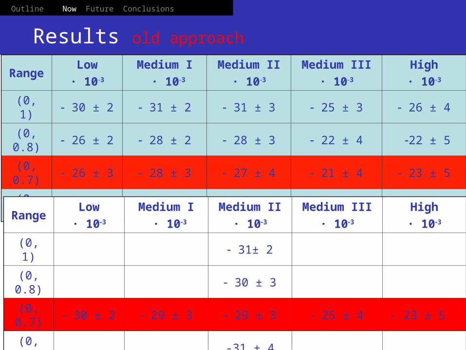
Results old approach
Frascati 29 September 2008
RangeLow
· 103Medium I
· 103Medium II
· 103Medium III
· 103High
· 103
(0, 1) 30 ± 2 31 ± 2 31 ± 3 25 ± 3 26 ± 4
(0, 0.8) 26 ± 2 28 ± 2 28 ± 3 22 ± 4 22 ± 5
(0, 0.7) 26 ± 3 28 ± 3 27 ± 4 21 ± 4 23 ± 5
(0, 0.6) 30 ± 4 31 ± 4 31 ± 4 24 ± 5 20 ± 6
RangeLow
· 103Medium I
· 103Medium II
· 103Medium III
· 103High
· 103
(0, 1) 31± 2
(0, 0.8) 30 ± 3
(0, 0.7) 30 ± 2 29 ± 3 29 ± 3 25 ± 4 - 23 ± 5
(0, 0.6) -31 ± 4

Outline Now Future Conclusions
Ponza 05 June 2008
Fit procedure
ni log i i
We obtain an extimate by minimizingThe fit is done using a binned likelihood approach
Where:
ni = recostructed eventsi = for each MC event (according pure phase space): Evaluate its ztrue and its zrec (if any!) Enter an histogram with the value of zrec
Weight the entry with 1 + 2 ztrue Weight the event with the fraction of combinatorial background, for the signal (bkg) if it has correct (wrong) pairing
Frascati 29 September 2008
Outline Now Future Conclusions
Ponza 05 June 2008
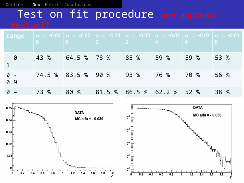
Test on fit procedure new approach MediumII
range
0 - 1 43 % 64.5 % 78 % 85 % 59 % 59 % 53 %
0 - 0.9 74.5 % 83.5 % 90 % 93 % 76 % 70 % 56 %
0 – 0.8 73 % 80 % 81.5 % 86.5 % 62.2 % 52 % 38 %
0 – 0.7 62 % 69 % 71 % 80 % 51 % 49 % 33 %
0 – 0.6 32 % 66 % 72 % 78 % 68 % 63 % 45 %

Outline Now Future Conclusions
Ponza 05 June 2008
Test on fit procedure
Hit or Miss fit procedure

Outline Now Future Conclusions
Ponza 05 June 2008
Three new samples
Frascati 29 September 2008
LOWPur 90.02% Eff 30.48 %9.5 %Res 0.1421
MEDIUMPur 95.6% Eff 20.92 %13.11 %Res 0.1234
HIGHPur 97.42% Eff 16 %9 %Res 0.1177

Outline Now Future Conclusions
Ponza 05 June 2008
Wrong Pairing fit old vs. new approach
MEDIUM MEDIUM
HIGH HIGH
Old approach New approach
LOW
Old approach New approach
Old approach New approach
LOW

Outline Now Future Conclusions
Ponza 05 June 2008
Results old vs. new approach
Frascati 29 September 2008
91 % 43 % 66 %
(0, 0.6) 30 ± 4 29 ± 5 24 ± 4
83 % 28 % 52 %
Range
PLow
· 103Medium
· 103HIGH
· 103
(0, 1) 27 ± 2 26 ± 2 22 ± 3
96 % 62 % 73 %
(0, 0.7) 28 ± 3 25 ± 4 22 ± 4
8 % 3 % 0.1 %
(0, 0.6) 46 ± 2 53 ± 3 54 ± 4
2 % 2 % 3 %
RangeLow
· 103Medium
· 103HIGH
· 103
(0, 1) 41 ± 3 46 ± 2 44 ± 3
6 % 2 % 0.1 %
(0, 0.7) 46 ± 4 46 ± 3 47 ± 4

Outline Now Future Conclusions
Ponza 05 June 2008
Residuals old vs. new approach
HIGH OLD approach
HIGH NEW approach
MEDIUM NEW approach
MEDIUM OLD approach
LOW NEW approach
LOW NEW approach

Outline Now Future Conclusions
Ponza 05 June 2008
Future plans & conclusions
Frascati 29 September 2008
In order to understand the presence of the slope in the wrong pairing fit : Introduce in the kinematic fit procedure the √s run by run
Use the MC samples with different values to fit the w.p.
If do you have other ideas?... They are very welcomes.

Introduction Analysis Results Conclusions
Ponza 05 June 2008
Zgen in acceptance
Frascati 29 September 2008

Introduction Analysis Results Conclusions
Ponza 05 June 2008
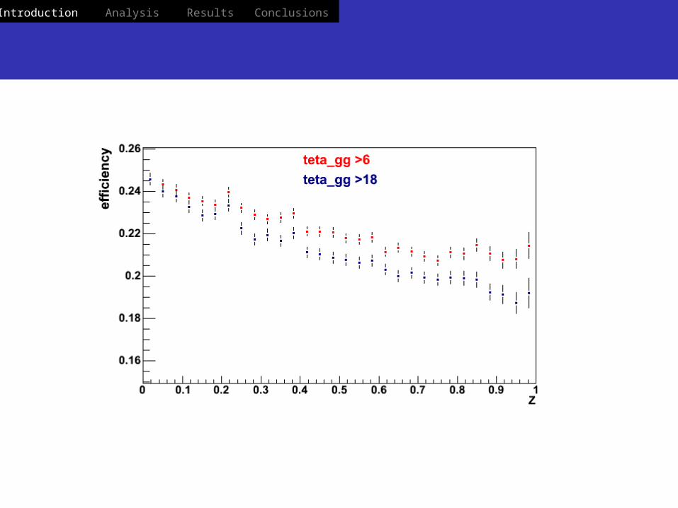
Efficienza con i diversi tagli in sample Medium II
Frascati 29 September 2008
Introduction Analysis Results Conclusions
Ponza 05 June 2008

Introduction Analysis Results Conclusions
Ponza 05 June 2008
Da confrontare con i risultati dalla procedura di fit
Medium II
· 103
37 ± 2
34 ± 3
36 ± 3
42 ± 4
Medium II
· 103
32 ± 2
28 ± 3
27 ± 3
38 ± 3
Range
(0, 1)
(0, 0.8)
(0, 0.7)
(0, 0.6)
Ripesando per il BKG
Nonripesando per il BKG
Introduction Analysis Results Conclusions
Status report on analysisPonza 05 June 2008
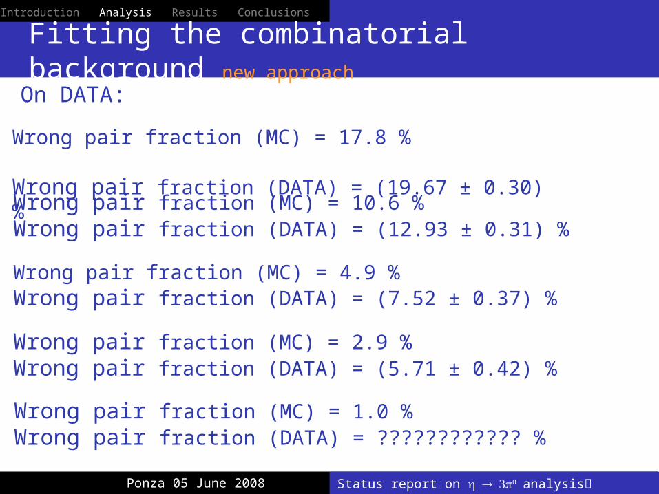
Fitting the combinatorial background new approach
On DATA:
Wrong pair fraction (MC) = 10.6 %Wrong pair fraction (DATA) = (12.93 ± 0.31) %
Wrong pair fraction (MC) = 4.9 %Wrong pair fraction (DATA) = (7.52 ± 0.37) %
Wrong pair fraction (MC) = 2.9 %Wrong pair fraction (DATA) = (5.71 ± 0.42) %
Wrong pair fraction (MC) = 1.0 %Wrong pair fraction (DATA) = ???????????? %
Wrong pair fraction (MC) = 17.8 % Wrong pair fraction (DATA) = (19.67 ± 0.30) %

Status report on analysisPonza 05 June 2008
Results Old – New
RangeLow
· 103Medium I
· 103Medium II
· 103Medium III
· 103High
· 103
(0, 1) 30 ± 2 31 ± 2 31 ± 3 25 ± 3 26 ± 4
(0, 0.8) 26 ± 2 28 ± 2 28 ± 3 22 ± 4 22 ± 5
(0, 0.7) 26 ± 3 28 ± 3 27 ± 4 21 ± 4 23 ± 5
(0, 0.6) 30 ± 4 31 ± 4 31 ± 4 24 ± 5 20 ± 6
RangeLow
· 103Medium I
· 103Medium II
· 103Medium III
· 103High
· 103
(0, 1) 36 ± 2 37 ± 2 37 ± 2 35 ± 3
(0, 0.8) 36 ± 2 37 ± 2 34 ± 3 32 ± 3
(0, 0.7) 38 ± 2 40 ± 3 36 ± 3 33 ± 3
(0, 0.6) 44 ± 3 48 ± 4 42 ± 4 37 ± 4
Introduction Analysis Results Conclusions

Introduction Analysis Results Conclusions
Ponza 05 June 2008
Residui old – new approach
Status report on analysis
HIGH OLD approach
HIGH NEW approach
MEDIUM NEW approach
MEDIUM OLD approach

Introduction Analysis Results Conclusions
Ponza 05 June 2008
Residui old – new approach
Status report on analysis
LOW NEW approach
LOW OLD approach

Introduction Analysis Results Conclusions
Ponza 05 June 2008
Test con nuovo taglio in P(2)
Status report on analysis
Taglio finora utilizzatoP(2) > 0.012 < 25
Taglio nuovoP(2) > 0.12 < 19
Cosa succede al fondo……

Introduction Analysis Results Conclusions
Ponza 05 June 2008
Test con nuovo taglio in P(2) new approach
Status report on analysis
HIGH
MEDIUM MEDIUM

Introduction Analysis Results Conclusions
Ponza 05 June 2008
Test con nuovo taglio in P(2) new approach
Status report on analysis
LOWLOW
…. Purtroppo non è cambiato niente!!!!!

E1
E2
E
Introduction Analysis Results Conclusions
Status report on analysisPonza =5 June 2008
Systematic on Resolution
A further check can be done comparing the energies of the two photons in the pion rest frame as function of pion energy
Vs.

Introduction Analysis Results Conclusions
Statu report on analysisPonza 05 June 2008
Systematic on Resolution
Stefano ha chiesto di •confrontare il valor medio e la sigma del fit gaussiano,•graficare le diverse slices per il wrong e right pairing (versione cartacea) •Mettere in tabella Ncore e Ntail
A further check can be done comparing the energies of the two photons in the pion rest frame as function of pion energy

Introduction Analysis Results Conclusions
Ponza 05 June 2008
valor medi campioni low e High new approach
Status report on analysis
Low
MCDATA
MCDATA
High

Introduction Analysis Results Conclusions
Ponza 05 June 2008
sigma campioni low e High new approach
Status report on analysis
MCDATA
MCDATA
Low High La discrepanza potrebbe essere dovuta al fatto che io ho fatto un fit con 3gaus e ho plottato solo la di core, avrei dovuto tenere conto delle altre opportunamentepesate per Ni

Introduction Analysis Results Conclusions
Ponza 05 June 2008
Tabella Ncore Ntails
Status report on analysis
MC
Ncore Ntails
361 146
1494 1064
1458 1554
3095 1806
3749 1972
3991 2078
4129 2062
3852 1690
2920 1303
744 393
DATA
Ncore Ntails
86 42
399 264
558 532
828 517
930 571
1055 587
1063 549
932 476
761 315
197 128
195 133
Campione MEDIUM

Introduction Analysis Results Conclusions
Ponza 05 June 2008
Plot vari
Status report on analysis
Ho solo la copia cartacea dei vari check effettuati…

Introduction Analysis Results Conclusions
Ponza 05 June 2008
SPARE SLIDES
Status report on analysis

Status report on analysisPonza 05 June 2008
Sample selection
OLD approach:
7 and only 7 pnc with 21° < < 159° and E > 10 MeV > 18° Kin Fit with no mass constraint P(2) > 0.01 320 MeV < Erad < 400 MeV AFTER PHOTON’S PAIRINGKinematic Fit with and mass
constraints (on DATA M= 547.822
MeV/c2 )
NEW approach:
7 and only 7 pnc with 21° < < 159° and E > 10 MeV > 18° Kin Fit with mass constraint
(on DATA M= 547.874 MeV/c2 ) P(2) > 0.01 320 MeV < Erad < 400 MeV AFTER PHOTON’S PAIRINGKinematic Fit with mass constraint
Introduction Analysis Results Conclusions

Status report on analysisPonza 05 June 2008
Purity Old – New
Using the same cuts on min and
Pur 75.4%
Pur 84.5%
Pur 92%
Pur 94.8%
Pur 97.6%
Pur 82.2%
Pur 99%
Pur 97.1%
Pur 95.1%
Pur 89.4%
Low purity
Medium I purity
Medium II purity
Medium III purity
High purity
Introduction Analysis Results Conclusions
Status report on analysisPonza 05 June 2008
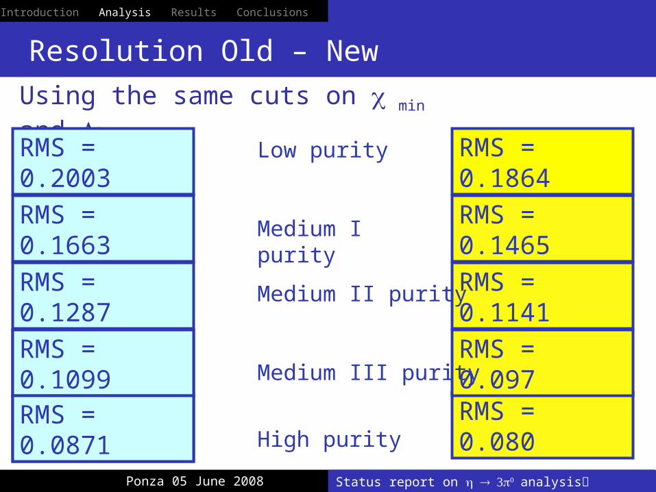
Resolution Old – New
Using the same cuts on min and
RMS = 0.2003
RMS = 0.1663
RMS = 0.1287
RMS = 0.2003
RMS = 0.1864
RMS = 0.080
RMS = 0.097
RMS = 0.1141
RMS = 0.1465
Low purity
Medium I purity
Medium II purity
Medium III purity
High purity
RMS = 0.1099
RMS = 0.0871
Introduction Analysis Results Conclusions

Status report on analysisPonza 05 June 2008
Resolution (Medium II sample )
Introduction Analysis Results Conclusions

Status report on analysisPonza 05 June 2008
Efficiency Old – New
Using the same cuts on min and
= 22.02 %
= 13.64 %
= 9.24 %
= 4.34%
= 30.15 %
6.60%
= 11.76%
= 16.24%
= 23.69 %
Low purity
Medium I purity
Medium II purity
Medium III purity
High purity
Introduction Analysis Results Conclusions
Status report on analysisPonza 05 June 2008
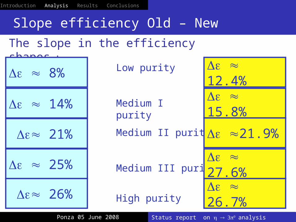
Slope efficiency Old – New
The slope in the efficiency shapes
8%
14%
21%
25%
26%
Low purity
Medium I purity
Medium II purity
Medium III purity
High purity
12.4%
15.8%
21.9%
27.6%
26.7%
Introduction Analysis Results Conclusions

Status report on analysisPonza 05 June 2008
Efficiency (Medium II sample)
Introduction Analysis Results Conclusions

Introduction Analysis Results Conclusions
Status report on analysisPonza 05 June 2008
Fitting the combinatorial background (Old)
On DATA:
Wrong pair fraction (MC) = 15.5 %Wrong pair fraction (DATA) = (16.7 ± 0.28) %
Wrong pair fraction (MC) = 7.9 %Wrong pair fraction (DATA) = (8.98 ± 0.37) %
Wrong pair fraction (MC) = 5.2 %Wrong pair fraction (DATA) = (5.2 ± 0.45) %
Wrong pair fraction (MC) = 2.4 %Wrong pair fraction (DATA) = (3.47 ± 1.00) %
Wrong pair fraction (MC) = 24.6 % Wrong pair fraction (DATA) = (26.45 ± 0.26) %

Introduction Analysis Results Conclusions
Status report on analysisPonza 05 June 2008
Fitting the combinatorial background (New)
On DATA:
Wrong pair fraction (MC) = 10.6 %Wrong pair fraction (DATA) = (12.86 ± 1.14) %
Wrong pair fraction (MC) = 4.9 %Wrong pair fraction (DATA) = (7.21 ± 1.37) %
Wrong pair fraction (MC) = 2.9 %Wrong pair fraction (DATA) = (5.09 ± 1.69) %
Wrong pair fraction (MC) = 1.0 %Wrong pair fraction (DATA) = ???????????? %
Wrong pair fraction (MC) = 17.8 % Wrong pair fraction (DATA) = (19.16 ± 1.10) %

Introduction Analysis Results Conclusions
Status report on analysisPonza 05 June 2008
Fit procedure
ni log i i
We obtain an extimate by minimizingThe fit is done using a binned likelihood approach
Where:
ni = recostructed eventsi = for each MC event (according pure phase space): Evaluate its ztrue and its zrec (if any!) Enter an histogram with the value of zrec
Weight the entry with 1 + 2 ztrue Weight the event with the fraction of combinatorial background, for the signal (bkg) if it has correct (wrong) pairing

Introduction Analysis Results Conclusions
Status report on analysisPonza 05 June 2008
The systematic check
This procedure relies heavily on MC.
The crucial checks for the analysis can be summarizedin three main questions:
I. Is MC correctly describing efficiencies ?II. Is MC correctly describing resolutions ?III. Is MC correctly estimating the “background” ?

Introduction Analysis Results Conclusions
Status report on analysisPonza 05 June 2008
Efficiency (I)
Correction to the photon efficiency is applied weighting the Montecarloevents for the Data/MC photon efficiency ratio ≈ 1 exp(E/8.1)

Introduction Analysis Results Conclusions
Status report on analysisPonza 05 June 2008
Efficiency (I) (Medium II sample)
Correction to the photon efficiency is applied weighting the Montecarloevents for the Data/MC photon efficiency ratio ≈ 1 exp(E/8.1)

Introduction Analysis Results Conclusions
Status report on analysisPonza 05 June 2008
Efficiency (II)
Further check is to look at the relative ratio between the different samples:
N2/N1 data = 0.7888 ± 0.0010
N3/N1 data = 0.5466 ± 0.0008
N4/N1 data = 0.3988 ± 0.0006
N5/N1 data = 0.2273 ± 0.0004
N2/N1 mc = 0.7859 ±0.0007
N3/N1 mc = 0.5382 ±0.0006
N4/N1 mc = 0.3894 ±0.0005
N5/N1 mc. = 0.2188 ±0.0003

Introduction Analysis Results Conclusions
Status report on analysisPonza 05 June 2008
Resolution (I)
Introduction Analysis Results Conclusions
Status reort on analysisPonza 05 June 2008
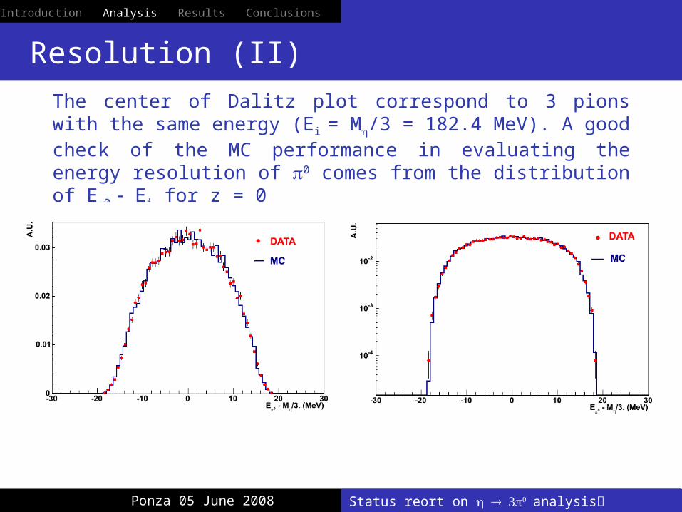
Resolution (II)
The center of Dalitz plot correspond to 3 pions with the same energy (Ei = M/3 = 182.4 MeV). A good check of the MC performance in evaluating the energy resolution of 0 comes from the distribution of E0 Ei for z = 0

E1
E2
E
Introduction Analysis Results Conclusions
Status report on analysisPonza =5 June 2008
Resolution (III)
A further check can be done comparing the energies of the two photons in the pion rest frame as function of pion energy
Vs.

Introduction Analysis Results Conclusions
Statu report on analysisPonza 05 June 2008
Resolution (IV)
A data MC discrepancy at level of 12 % is observed.Thus we fit filling a histo with: z’rec = zgen + (zrec zgen ).
A further check can be done comparing the energies of the two photons in the pion rest frame as function of pion energy

Introduction Analysis Results Conclusions
Status report on analysisPonza 05 June 2008
Background Old
Background composition, Medium II purity sample

Introduction Analysis Results Conclusions
Status report on analysisPonza 05 June 2008
Background Old

Introduction Analysis Results Conclusions
Status report on analysisPonza 05 June 2008
Background New
Background composition, Medium II purity sample

Introduction Analysis Results Conclusions
Status report on analysisPonza 05 June 2008
Background New
Status report on analysisPonza 05 June 2008
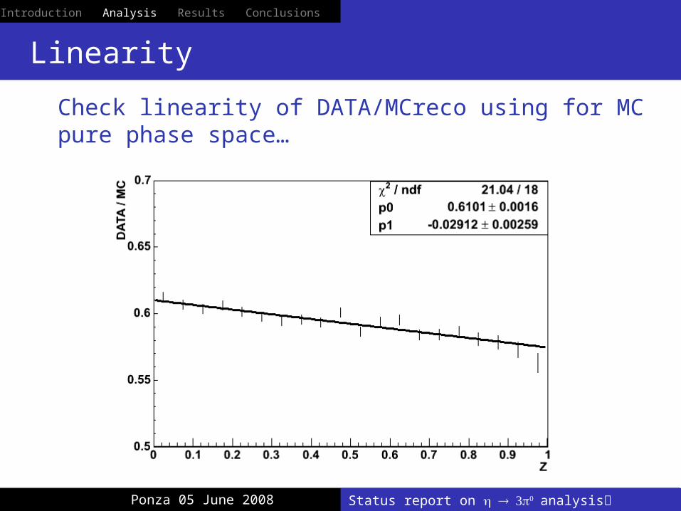
Linearity
Check linearity of DATA/MCreco using for MC pure phase space…
Introduction Analysis Results Conclusions

Status report on analysisPonza 05 June 2008
Results Old – New
RangeLow
· 103Medium I
· 103Medium II
· 103Medium III
· 103High
· 103
(0, 1) 30 ± 2 31 ± 2 31 ± 3 25 ± 3 26 ± 4
(0, 0.8) 26 ± 2 28 ± 2 28 ± 3 22 ± 4 22 ± 5
(0, 0.7) 26 ± 3 28 ± 3 27 ± 4 21 ± 4 23 ± 5
(0, 0.6) 30 ± 4 31 ± 4 31 ± 4 24 ± 5 20 ± 6
RangeLow
· 103Medium I
· 103Medium II
· 103Medium III
· 103High
· 103
(0, 1) 36 ± 2 37 ± 2 37 ± 2 35 ± 3
(0, 0.8) 36 ± 2 37 ± 2 34 ± 3 32 ± 3
(0, 0.7) 38 ± 2 40 ± 3 36 ± 3 33 ± 3
(0, 0.6) 44 ± 3 48 ± 4 42 ± 4 37 ± 4
Introduction Analysis Results Conclusions

Status report on analysisPonza 05 June 2008
Systematic uncertainties Old - New
EffectLow
· 103Medium I
· 103Medium II
· 103Medium III
· 103High
· 103
Res 9 6 4 3 3
Low E 1.6 1.9 1.6 1.3 1.4
Bkg 0. 0. 0. 1 1 +1
M 1 1 2 2 5
Range 4 3 4 4 3 +3
Purity 2 +5 +7 1 + 6 7 5 + 2
Tot 10 + 5 7 + 7 6 + 6 9 9 + 4
EffectLow
· 103Medium I
· 103Medium II
· 103Medium III
· 103
Res - 4 - 4 - 2 - 2
Low E negligible negligible negligible negligible
Bkg 3. -1 +3 -3 2
M 1 +1 0 0 1 +1
Range -6 + 2 8 +3 6 +2 -4 + 1
Purity -2 +5 +7 4 + 3 7
Tot 8 + 6 9 + 8 8 + 4 9 + 1
Introduction Analysis Results Conclusions

Status report on analysisPonza 05 June 2008
Data / Fit distribution New
Introduction Analysis Results Conclusions
Status report on analysisPonza 05 June 2008
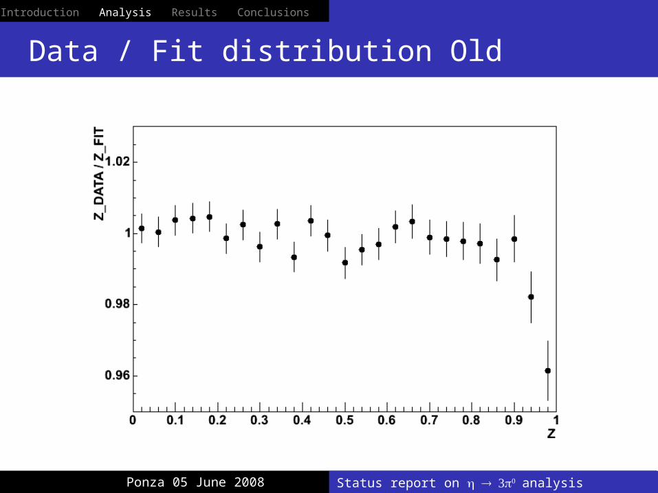
Data / Fit distribution Old
Introduction Analysis Results Conclusions

Status report of analysisPonza 05 June 2008
Results No bkg - bkg
RangeLow
· 103Medium I
· 103Medium II
· 103Medium III
· 103
(0, 1) 33 ± 2 33 ± 2 32 ± 2 29 ± 3
(0, 0.8) 32 ± 2 30 ± 2 28 ± 3 25 ± 3
(0, 0.7) 32 ± 2 31 ± 3 27 ± 3 24 ± 3
(0, 0.6) 36 ± 4 24 ± 3 38 ± 3 25 ± 4
RangeLow
· 103Medium I
· 103Medium II
· 103Medium III
· 103
(0, 1) 36 ± 2 37 ± 2 37 ± 2 35 ± 3
(0, 0.8) 36 ± 2 37 ± 2 34 ± 3 32 ± 3
(0, 0.7) 38 ± 2 40 ± 3 36 ± 3 33 ± 3
(0, 0.6) 44 ± 3 48 ± 4 42 ± 4 37 ± 4
Introduction Analysis Results Conclusions

Status report on analysisPonza 05 June 2008
Systematic uncertainties No bkg - bkg
EffectLow
· 103Medium I
· 103Medium II
· 103Medium III
· 103
Res
Low E
Bkg
M
Range -4 2 +7 11 -5
Purity +8 -1 +7 5 + 3 8
Tot 4 + 8 2 + 10 12 + 3 9
EffectLow
· 103Medium I
· 103Medium II
· 103Medium III
· 103
Res - 4 - 4 - 2 - 2
Low E negligible negligible negligible negligible
Bkg 3. -1 +3 -3 2
M 1 +1 0 0 1 +1
Range -6 + 2 8 +3 6 +2 -4 + 1
Purity -2 +5 +7 4 + 3 7
Tot 8 + 6 9 + 8 8 + 4 9 + 1
Introduction Analysis Results Conclusions

Status report on analysisPonza 05 June 2008
Data / Fit distribution
Introduction Analysis Results Conclusions

Introduction Analysis Results Conclusions
Status report on analysisPonza 05 June 2008
Summary
Using the Old approach, we have published this preliminary results:
This result is compatible with the published Crystal Ball result: = 0.031 ± 0.004
And the calculations from the +- analysis using only the - rescattering in the final state.
= 0.027 ± 0.004stat ± 0.006 syst
= 0.038 ± 0.003stat +0.012
-0.008 syst
Using the New approach we have:
0.027< < 0.036

Introduction Theoretical tools Results Conclusions
Status report on analysisPonza 05 June 2008
Conclusions

Introduction Theoretical tools Results Conclusions
Ponza 05 June 2008
Spare
Status report on analysis
Introduction Theoretical tools Results Conclusions
Ponza 05 June 2008
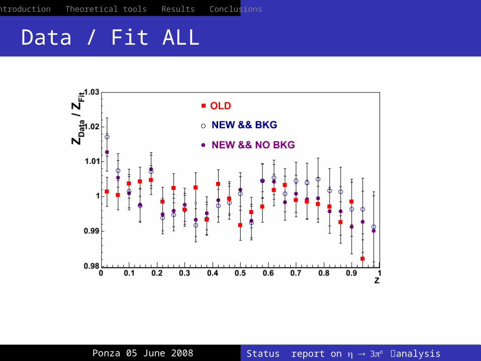
Data / Fit ALL
Status report on analysis

Introduction Analysis Results Conclusions
Ponza 05 June 2008
Background Old - New
Status report on analysis

Status of analysis
F. Ambrosino T. Capussela F. Perfetto
Status of analysisPonza 05 June 2008

Status of analysis
Conclusions: 12 March 2008
We have to resolve the Data MC discrepancy on min
2
We are ready to fit and to evaluate the systematical errors in the NEW approach.
Ponza 05 June 2008

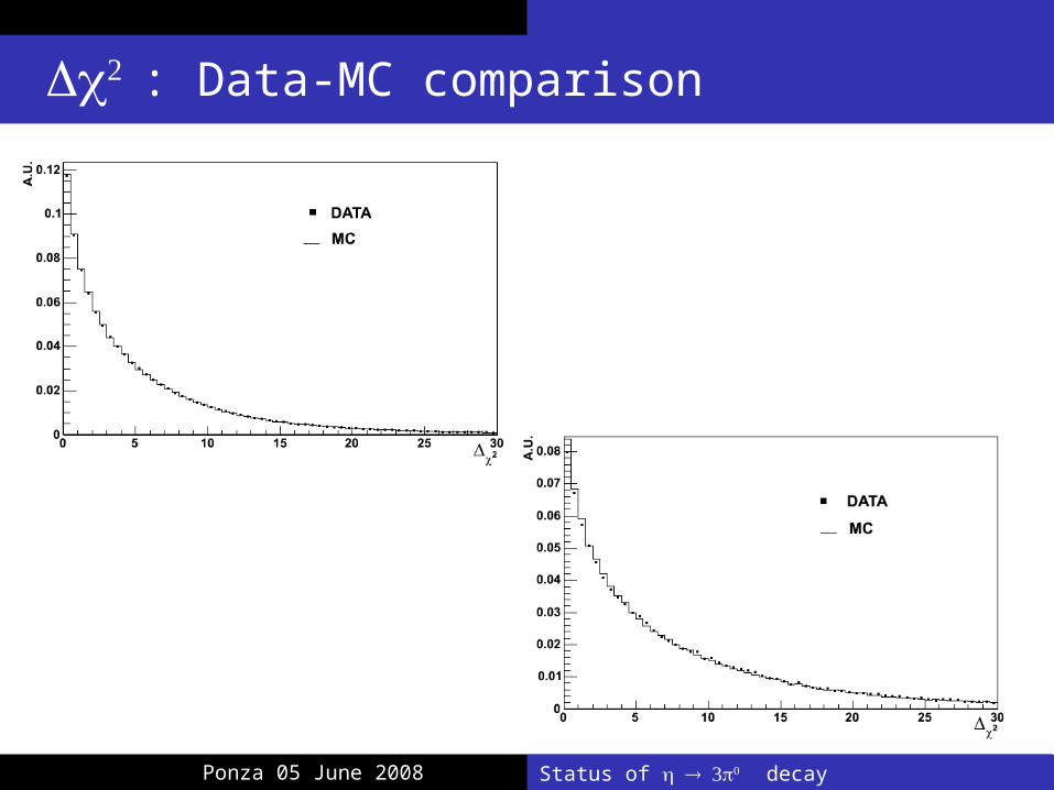
Status of analysis
min : Data-MC comparison
Ponza 05 June 2008

Status of analysis
min
m0
j
m ioj
j2
m i
0j M
0
m0
j
i1
3
2
Recoil is the most energetic cluster.In order to match every couple of photon to the right 0 we build a 2-like variable for each of the 15 combinations:
With:
is the invariant mass of i0 for j-th combination
= 134.98 MeV
is obtained as function of photon energies
M 0
Ponza 05 June 2008

Status of decayFrascati 14 May 2008
min : Data-MC comparison

Introduction Analysis Results Conclusions
Status of analysis
Energy resolution
EEp1 1 e
p2
E p3
Ep4
E
MM
1
2
E1
E1
E2
E2
We have corrected the for the observed Data-MC discrepancy
Ponza 05 June 2008

Status of analysis
Sample selection
OLD approach:
7 and only 7 pnc with 21° < < 159° and E > 10 MeV > 18° Kin Fit with no mass constraint P(2) > 0.01 320 MeV < Erad < 400 MeV AFTER PHOTON’S PAIRINGKinematic Fit with and mass
constraints (on DATA M=547.822
MeV/c2 )
NEW approach:
7 and only 7 pnc with 21° < < 159° and E > 10 MeV > 18° Kin Fit with mass constraint
(on DATA M= 547.822 MeV/c2 ) P(2) > 0.01 320 MeV < Erad < 400 MeV AFTER PHOTON’S PAIRINGKinematic Fit with mass constraint
Ponza 05 June 2008

Status of analysis
OLD – NEW results
RangeLow
· 103Medium I
· 103Medium II
· 103Medium III
· 103High
· 103
(0, 1) 30 ± 2 31 ± 2 31 ± 3 25 ± 3 26 ± 4
(0, 0.8) 26 ± 2 28 ± 2 28 ± 3 22 ± 4 22 ± 5
(0, 0.7) 26 ± 3 28 ± 3 27 ± 4 21 ± 4 23 ± 5
(0, 0.6) 30 ± 4 31 ± 4 31 ± 4 24 ± 5 20 ± 6
RangeLow
· 103Medium I
· 103Medium II
· 103Medium III
· 103High
· 103
(0, 1) 36 ± 2 37 ± 2 37 ± 2 35 ± 3
(0, 0.8) 36 ± 2 37 ± 2 34 ± 3 32 ± 3
(0, 0.7) 38 ± 2 40 ± 3 36 ± 3 33 ± 3
(0, 0.6) 44 ± 3 48 ± 4 42 ± 4 37 ± 4
Ponza 05 June 2008

Introduction Theoretical tools Results Conclusions
Dalitz plot analysis of with the KLOE experiment
OLD – NEW systematic uncertainties
EffectLow
· 103Medium I
· 103Medium II
· 103Medium III
· 103High
· 103
Res 9 6 4 3 3
Low E 1.6 1.9 1.6 1.3 1.4
Bkg 0. 0. 0. 1 1 +1
M 1 1 2 2 5
Range 4 3 4 4 3 +3
Purity 2 +5 +7 1 + 6 7 5 + 2
Tot 10 + 5 7 + 7 6 + 6 9 9 + 4
EffectLow
· 103Medium I
· 103Medium II
· 103Medium III
· 103
Res ???? ???? + 5 ?????
Low E 0.2 0.1 .2 0.4
Bkg 3. -1 +3 -3 2
M 1 +1 0 0 1 +1
Range -6 + 2 8 +3 6 +2 -4 + 1
Purity -2 +5 +7 4 + 3 7
Tot 6 + 6 8 + 8 8 + 6 8 +1Ponza 05 June 2008

Status of analysis
OLD – NEW result
In the OLD approach we give the final result for the slope parameter in corrispondence of the sample with 92% of purity (Medium II):
= 0.027 ± 0.004stat ± 0.006 syst
In the NEW approach we give the final result for the slope parameter in corrispondence of the sample with 95% of purity (MediumII):
= 0.036 ± 0.003stat - 0.008/+0.006 syst
Ponza 05 June 2008

Status of analysis
OLD - NEW
Using the same cuts on min and
Pur 75.4%
Pur 84.5%
Pur 92%
Pur 94.8%
Pur 97.6%
Pur 82.2%
Pur 99%
Pur 97.1%
Pur 95.1%
Pur 89.4%
Low purity
Medium I purity
Medium II purity
Medium III purity
High purity
Ponza 05 June 2008

Status of analysis
OLD - NEW
The slope in the efficiency shapes
8%
14%
21%
25%
26%
Low purity
Medium I purity
Medium II purity
Medium III purity
High purity
12.4%
15.8%
21.9%
27.6%
26.7%
Ponza 05 June 2008

Status of analysis
OLD - NEW
RMS = 0.1169
RMS = 0.1632
Ponza 05 June 2008
Status of decay
: Data-MC comparison
Ponza 05 June 2008