pontificia universidad catolica de chile ......estructura de khace que, o bien la teor a di era...
TRANSCRIPT

PONTIFICIA UNIVERSIDAD CATOLICA DE CHILEFACULTAD DE MATEMATICAS
CALCULO ULTRAMETRICO SOBRE UN CUERPO K CONUNA VALUACION DE RANGO INFINITO
por
Hector Moreno Barrera
Tesis presentada a la Facultad de Matematicasde la Pontificia Universidad Catolica de Chile
para optar al grado de Doctor en Matematicas.
Profesor Guıa: Herminia Ochsenius Alarcon.
Comision Informante: Wim SchikhofJuan Rivera-LeterierClaudio Fernandez
Diciembre, 2013Santiago, Chile
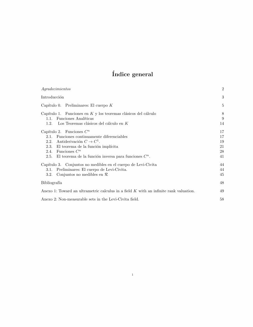
Indice general
Agradecimientos 2
Introduccion 3
Capıtulo 0. Preliminares: El cuerpo K 5
Capıtulo 1. Funciones en K y los teoremas clasicos del calculo 81.1. Funciones Analıticas 91.2. Los Teoremas clasicos del calculo en K 14
Capıtulo 2. Funciones Cn 172.1. Funciones continuamente diferenciables 172.2. Antiderivacion C → C1. 192.3. El teorema de la funcion implıcita 212.4. Funciones Cn 282.5. El teorema de la funcion inversa para funciones Cn. 41
Capıtulo 3. Conjuntos no medibles en el cuerpo de Levi-Civita 443.1. Preliminares: El cuerpo de Levi-Civita. 443.2. Conjuntos no medibles en R 45
Bibliografıa 48
Anexo 1: Toward an ultrametric calculus in a field K with an infinite rank valuation. 49
Anexo 2: Non-measurable sets in the Levi-Civita field. 58
1

Agradecimientos
A mi familia, por el amor infinito que me han entregado y los sacrificios que han hecho por mı entodos estos anos. Por el apoyo y comprension que han sido fundamentales en toda mi vida estudiantil.
A mi profesora guıa Herminia Ochsenius, por todos las ensenanzas, consejos, apoyo y la confianzaque siempre deposito en mı.
A los profesores Claudio Fernandez y Juan Rivera-Letelier por aceptar leer cuidadosamente mitesis e integrar la comision informante.
A Conicyt, por haberme otorgado la beca de estudios de Doctorado en Chile.
A la Vicerrectoria de Investigacion de la PUC, por sus becas de Ayudante e Instructor Becario.
Quiero agradecer en especial al profesor Wim Schikhof, por sus colaboraciones, consejos y sugeren-cias fueron muy importantes durante mis estudios de doctorado. A pesar de las difıciles circunstancias,tuvo la disposicion de leer cuidadosamente mi tesis y de haber integrado la comision informante.

Introduccion
En 1980, H. Keller construye el primer espacio de tipo Hilbert sobre un cuerpo K distinto de R. Esinfinito dimensional, completo en la topologıa de la norma inducida por un producto interno, y en eles valido el teorema de Proyeccion. Son las caracterısticas algebraicas de K: su orden no arquimedianoy la estructura del grupo cuociente K+\(K+)2, las que permitieron la construccion del espacio (ver[4]). Pero la investigacion hasta la fecha se ha centrado en los espacios de tipo Hilbert, y no se harealizado un estudio de K desde el punto de vista del calculo y analisis ultrametrico, que es el temade esta Tesis.
Por otra parte K admite una valuacion no arquimediana, cuyo grupo de valores Γ, linealmente ordenadopor ≤, es la union de una sucesion estrictamente creciente de subgrupos cada uno de los cuales es unsubconjunto convexo del grupo. Esto es, la valuacion de K es de rango infinito. A partir de los estudiosen cuerpos p-adicos hay muchos y profundos estudios centrados en el analisis en cuerpos valuadoscon grupo de valores isomorfo a un subgrupo de (R+, ·) (valuaciones de rango 1). En particular seesta desarrollando una teorıa sobre uno de ellos, el cuerpo de Levi-Civita, que es ademas real cerrado.Sobre cuerpos con valuaciones de rango infinito hay pocos trabajos, y en general se les pide quesean algebraicamente cerrados (y por tanto no ordenables). Esta tesis esta en deuda con todos ellos,en particular con el libro Ultrametric Calculus de W. Schikhof, en tanto que han presentado lıneasde estudio y desarrollado nuevos conceptos para abordar las dificultades que se presentan. Pero laestructura de K hace que, o bien la teorıa difiera sustancialmente de los resultados allı obtenidos, obien que ellos sean validos, pero con demostraciones diferentes. En particular, aquı el interjuego entreel orden, la valuacion y la ultrametrica definida en K es central en la demostracion de los teoremas,ası como en la existencia de los numerosos contraejemplos a las versiones clasicas de los teoremas delcalculo y analisis.
Se adjuntan como Anexos a la Tesis los dos artıculos publicados en la serie Contemporary Mathematics.Los teoremas demostrados en ellos se citan aquı sin demostracion.
En los Preliminares se describe el cuerpo K. El capıtulo 1 se centra en las funciones analıticas, cuyocomportamiento difiere tanto del caso clasico como del correspondiente a los cuerpos con valuaciones derango 1. Puesto que K es ordenado tienen sentido los enunciados de teoremas sobre extremos relativos.Hay contraejemplos para ellos en el caso general de funciones continuas pero se puede demostrar suvalidez, con la excepcion del teorema de valor intermedio, en el caso de funciones analıticas.
El segundo capıtulo traslada a K la nocion de funciones Cn, desarrollada en [3], que es la version masexigente de la propiedad de ser continuamente diferenciables. En este marco se establece un teoremade funcion inversa, y en el caso n = 1 un teorema de funcion implıcita. Se discute tambien la existenciade antiderivadas.
El ultimo capıtulo tiene una historia distinta. Puesto que en cuerpos ordenados se pueden definirintervalos y su longitud, es natural pensar en medidas, hay una teorıa bien desarrollada en el cuerpo
3

INTRODUCCION 4
de Levi-Civita, que ha permitido establecer en forma natural un proceso de integracion (ver [6]). Alestudiar este trabajo pensando en la valuacion no arquimediana de ese cuerpo surgio la pregunta por lamedida de la bola unitaria. Se pudo establecer que ella no es medible, y como consecuencia, que todointervalo (a, b) en Levi-Civita contiene infinitos subconjuntos convexos no medibles, en agudo contrastecon el caso clasico. El trabajo fue publicado recientemente y constituye el Anexo 2 cuyo resumen eseste capıtulo.

Capıtulo 0
Preliminares: El cuerpo K
El cuerpo K que constituye un objeto central en esta investigacion, es ordenado, posee una valuacion derango infinito y es ultrametrizable. Resumimos aquı los resultados obtenidos en la seccion Preliminaresde [1], y damos la notacion que sera usada en la Tesis.
Se construye primero el cuerpo F∞ adjuntando a R el conjunto de variables {Xi}i∈N, es decir,
F∞ :=
∞⋃
n=0
Fn
donde F0 := R, y Fn = Fn−1(Xn) si n ≥ 1.
Ordenamos F∞ en la forma siguiente. Consideramos F0 = R con el orden usual. Para n ≥ 1, el cuerpoFn = Fn−1(Xn) = F0(X1, X2, . . . , Xn) se ordena segun potencias de Xn: un polinomio P (Xn) =a0 + a1Xn + ... + asX
sn ∈ Fn−1[Xn] es positivo en Fn si y solo si as > 0 en Fn−1, y un cuociente de
polinomios λ =p(Xn)
q(Xn)es positivo en Fn si y solo si el polinomio p(Xn)q(Xn) lo es. Por tanto, F∞
tiene el orden inducido. Este orden es no arquimediano ya que N es un conjunto acotado, por ejemplopor X1. Ademas, induce el valor absoluto definido por |x| = max{x,−x}Este orden genera una topologıa en F∞ cuya base de vecindades del cero es la coleccion de conjuntosUε = {a ∈ F∞ : |a| < ε} para todo ε ∈ F∞.
Construiremos ahora una valuacion no arquimediana en F∞. Comenzamos definiendo su grupo devalores. Para cada i = 1, 2, 3, 4, ... escogemos un numero real gi > 1 y consideramos el subgrupo cıclicomultiplicativo Gi generado por gi con el orden usual de R. Definimos Γ como
Γ :=
{γ ∈ (gn1
1 , gn22 , gn3
3 , ..., gnii , ...) ∈
∞∏
i=1
Gi : ni ∈ Z y supp(γ) es finito
},
donde supp(γ) := {i ∈ N : ni 6= 0}. Γ es un grupo linealmente ordenado con la operacion componentea componente y con el orden antilexicografico, cuyo elemento identidad es 1 = (1, 1, 1, 1, 1, ...).
Para cada m ≥ 1 ponemos
Hm = G1 ×G2 × ...×Gm × {1} × {1} × ...y tenemos que {1} = H0 ⊂ H1 ⊂ H2 ⊂ ... son los subgrupos convexos de Γ. Por ello el grupo (y porextension, la valuacion que se define a continuacion) se dice de rango infinito. Esto lleva a una teorıacon diferencias importantes respecto al caso de rango 1. Allı el grupo de valores tiene como unicosubgrupo convexo propio a {1} y es por tanto isomorfo a un subgrupo de (R+, ·).Adjuntamos a Γ un menor elemento 0 que cumple 0 · g = g · 0 = 0. Definimos entonces la valuacion deKrull v : F∞ → Γ ∪ {0} como
5

0. PRELIMINARES: EL CUERPO K 6
1. v|R es la valuacion trivial,2. v(Xn) := (1, ..., 1, gn, 1, ...).
Notacion: En lo que sigue, usaremos con frecuencia gn := v(Xn), y por tanto g−1n = v( 1
Xn).
Para definir normas de funciones en K, necesitaremos la completacion por cortaduras de Dedekind deΓ, denotada por Γ#, sobre la cual actua Γ por
g · s = supΓ#
{gr : r ∈ G, r ≤ s},
para g ∈ Γ y s ∈ Γ#.
F∞ es ultrametrizable. En efecto, sea φ : F+∞ → R dada por φ(0) = 0, y
φ(x) = 2−mın{m∈N: X−1m ≤x}
si x 6= 0. De forma directa se verifica que la funcion d : F∞×F∞ → R+ definida por d(x, y) = φ(|x−y|)es ultrametrica en F∞.
Definicion 0.0.1. El cuerpo K es la completacion del espacio ultrametrico (F∞, d), su topologıase denotara por τ .
Las afirmaciones siguientes se demuestran en [1]:
El orden ≤, la valuacion v y la ultrametrica d definen la misma topologıa en F∞. Mas aun,(F∞, d), (F∞,≤) y (F∞, v) definen las mismas sucesiones de Cauchy.
La valuacion v de F∞ se extiende a K y (K, v) es un cuerpo valuado completo.
El orden ≤ de F∞ se extiende a K y (K,≤) es un cuerpo ordenado completo.
Las topologıas definidas en K por las extensiones de la valuacion y del orden coinciden con τ . Enparticular, se tienen las inclusiones:
{y ∈ K : d(x, y) <1
2n+1} ⊂ {y ∈ K : |x− y| < 1
Xn} ⊂ {y ∈ K : d(x, y) <
1
2n},
ası como
{y ∈ K : |x− y| < 1
Xn} ⊂ {y ∈ K : v(x− y) < g−1
n } ⊂ {y ∈ K : |x− y| < 1
Xn−1}.
Indicaremos a continuacion otros hechos basicos (ver [1], [4], o [5]):
Puesto que es inducida por una valuacion no arquimediana, τ es cero-dimensional y los con-juntos
Ba(r) = {x ∈ K : v(x− a) ≤ r}Ba(r−) = {x ∈ K : v(x− a) < r}
son abiertos y cerrados (clopen) en (K, τ) para todo a ∈ K y r ∈ Γ.
(K, τ) no es localmente compacto, pues
{x ∈ K : v(x) ≤ 1} =⋃
a∈R(a+ {x ∈ K : v(x) < 1}) =
⋃
a∈R{x ∈ K : v(x− a) < 1}
es un cubrimiento no numerable de B0(1) que no tiene subcubrimiento finito. Esto implica quela bola unitaria en K no es compacta.

0. PRELIMINARES: EL CUERPO K 7
K no es separable ya que R es un conjunto no numerable y discreto en K.
B0(1) es un anillo local cuyo ideal maximal es la bola B0(1−). Por lo tanto k := B0(1)/B0(1−)es el cuerpo residual asociado al subgrupo convexo {1}, y es isomorfo a R.
Por ser un cuerpo ordenado, K no es algebraicamente cerrado. Pero tampoco es real cerrado.
Observacion 0.0.2. La sucesion(
1Xn
)n
es coinicial en K+, por lo tanto converge a 0 en (K, τ).
Tambien la sucesion asociada g−1n = v( 1
Xn) tiende a 0 en Γ ∪ {0}. Este hecho se usara con frecuencia
en las acotaciones.
Puesto que K es un espacio (ultra)metrico, las definiciones de los conceptos basicos del calculo comolımites, continuidad, convergencias, etc, son las usuales. Equivalentemente, se expresaran en terminosde la valuacion o del orden.

Capıtulo 1
Funciones en K y los teoremas clasicos del calculo
Puesto que K es un cuerpo ordenado, es interesante plantear la pregunta sobre la validez de losteoremas del valor intermedio, valor medio, Rolle, entre otros. El problema es complejo ya que en estecaso tenemos un cuerpo que no es real cerrado y no es localmente compacto. Mostraremos primero,mediante contraejemplos, que versiones generales de estos teoremas no son validos. A continuacion seestudian las propiedades de las funciones analıticas en K. Los resultados centrales de este capıtulomuestran que en este caso las dificultades desaparecen.
Comenzamos con algunas definiciones previas.
Definicion 1.0.3. Sea X ⊂ K. Si f : X → K es una funcion acotada, definimos
‖f‖∞ = supΓ#
{v(f(x)) : x ∈ X}.
Definicion 1.0.4. Sea X ⊂ K y f : X → K una funcion. Diremos que f es localmente constanteen X si para cada punto a ∈ X existe una vencindad Va de a tal que f es constante en Va ∩X.
Teorema 1.0.5. Sea f : X → K una funcion continua, entonces, dado ε ∈ Γ, existe una funcionlocalmente constante g : X → K tal que v(f(z)− g(z)) < ε para todo z ∈ X.
Demostracion. La demostracion propuesta en [3] es valida para este caso. Se basa en probarque la relacion ∼ en X definida por
x ∼ y si v(f(x)− f(y)) < ε
es una relacion de equivalencia, cuyas clases de equivalencia son conjuntos Ui (i ∈ I) abiertos y cerradosa la vez (clopen). Luego, para cada i ∈ I se fija ai ∈ Ui y se define la funcion g : X → K como g(x) = aisi x ∈ Ui. Observamos que g es localmente constante en X y v(f(x)− g(x)) < ε para todo x ∈ X. �
Si f es localmente constante en X, entonces X admite una particion en conjuntos clopen Ui y f esconstante en cada Ui. Las funciones localmente constantes por tanto son continuas y con derivada 0en todo punto.
Ejemplo 1.0.6 (No se satisface el teorema del valor intermedio). Sea f : [0, 1]→ K definida porf(x) = x2. Observamos que f es continua en K y que f(0) < 1
X1< f(1). Pero X1 no es un cuadrado
en K, de lo contrario, si X1 = a2 para algun a ∈ K entonces (g1, 1, 1, . . .) = v(X1) = v(a)2 lo quecontradice la definicion de los elementos que contiene Γ.
Ejemplo 1.0.7 (Una funcion continua y acotada en un intervalo cerrado pero que no tiene maximoni mınimo). Sea J = B0(1−), por tanto el cuerpo residual k asociado al subgrupo convexo {1} es iguala
k = {a+ J : a ∈ R}.8

1.1. FUNCIONES ANALITICAS 9
La funcion f : [−X1, X1]→ K definida por
f(z) =
{a si z ∈ a+ J0 si no.
,
cumple las condiciones pedidas.
Ejemplo 1.0.8 (Un funcion diferenciable, no inyectiva y con derivada constante distinta de 0).Para cada n ∈ N con n ≥ 1 definimos los conjuntos
Bn =
{z ∈ K : v
(z − 1
Xn
)< g−1
2n
}.
Claramente los conjuntos Bn son clopen; ademas observamos que si z ∈ Bn para algun n ∈ N entoncesv(z) = g−1
n , lo que implica que Bn ∩Bm = ∅ si m 6= n. Definimos la funcion f : K → K como
f(z) =
{z − 1
X2nsi z ∈ Bn para algun n ∈ N.
z en otro caso.
Tenemos que f no es inyectiva en ninguna vecindad de 0, pues v( 1Xn− 1
X2n− 1
Xn) = v( 1
X2n) lo que
implica que
f
(1
Xn− 1
X2n
)=
1
Xn− 1
X2n= f
(1
Xn
).
La funcion g(z) = z − f(z) es localmente constante y por tanto diferenciable en K con derivada 0.Luego f es diferenciable, no es inyectiva en ninguna vecindad de 0 y f ′ ≡ 1.
En la ultima seccion de este capıtulo mostraremos que las dificultades desaparecen para el caso defunciones analıticas.
1.1. Funciones Analıticas
La mayorıa de los resultados que presentaremos en esta seccion fueron probados detalladamente en[1], por lo tanto solo daremos sus enunciados.
Definicion 1.1.1. Sea a0, a1, a2, . . . una sucesion en K. La serie de potencias
∞∑
j=0
ajzj es el lımite
de la sucesion s0(z), s1(z), . . . de polinomios en la variable z dados por sn(z) =
n∑
j=0
ajzj .
Como es usual, llamamos region de convergencia de la serie de potencias
∞∑
j=0
ajzj al conjunto {z ∈ K :
(sn(z))n converge}.
El teorema siguiente muestra la diferencia fundamental con el analisis clasico, ası como el del calculoultrametrico para cuerpos con valuacion de rango 1.
Teorema 1.1.2 ([1], 3.2). Una serie de potencias de la forma
∞∑
j=0
ajzj con aj ∈ K converge si y
solo si lımn→∞
an = 0.

1.1. FUNCIONES ANALITICAS 10
Corolario 1.1.3. Si S es la region de convergencia de una serie de potencias∞∑
j=0
aj(z − z0)j (z0 ∈ S)
entonces, o bien S = K, o bien S = {z0}.Senalamos una importante consecuencia del Teorema 1.1.2 que es la imposibilidad de definir las fun-ciones exponencial, logaritmo o trigonometricas como series de potencias en el sentido clasico, pues
por la definicion de v se tiene que v
(± 1
n!
)= 1 para todo n ∈ N \ {0}.
Teorema 1.1.4 ([1], 3.3). Sea
∞∑
n=0
anzn una serie de potencias que converge en K. Luego, para
cada a ∈ K la serie anterior converge uniformente en Ba(r) para todo r ∈ Γ. La funcion
x 7→∞∑
n=0
anzn (z ∈ K)
es diferenciable y su derivada es
x 7→∞∑
n=1
nanzn−1 (z ∈ K).
Definicion 1.1.5. Sea D ⊆ K abierto. Diremos que una funcion f : D → K es analıtica en Dsi existen elementos u ∈ D y a0, a1, . . . ∈ K tales que
f(z) =
∞∑
n=0
an(z − u)n (z ∈ D).
Teorema 1.1.6 ([1], 3.6). Sea f una funcion analıtica en un abierto D. Luego para cada v ∈ D
existen b0, b1, . . . ∈ K tales que f(z) =
∞∑
n=0
bn(z − v)n para todo z ∈ D.
Observamos que la continuacion analıtica es trivial en este caso. Por otro lado, si f es una funcionanalıtica en un abierto D, podemos extender f(z) para todo z ∈ K. Puesto que 0 ∈ K, el teorema
1.1.6 nos asegura que existen elementos a0, a1, a2, ... en K tales que f(z) =
∞∑
n=0
anzn para todo z ∈ K,
en particular, para todo z ∈ D. Concluımos que f(z) es una funcion analıtica en D si y solo si existena0, a1, . . . ∈ K tales que para cada z ∈ D
f(z) =
∞∑
n=0
anzn.
Al igual que en caso de funciones analıticas definidas sobre C, los ceros de una funcion analıtica noconstante no se pueden acumular. Mas aun, dada una bola B en K, una funcion analıtica f en K solopuede contener a lo mas un numero finito de ceros contenidos en B. Esta situacion se debe al siguienteteorema.
Teorema 1.1.7 ([1], 3.7). Sea f una funcion analıtica en un abierto D. Si existe una sucesion{zk}n∈N de puntos distintos en D con f(zk) = 0, entonces f ≡ 0 en D.

1.1. FUNCIONES ANALITICAS 11
Del mismo modo que en los casos clasicos y rango 1, se podrıa pensar que si f es analıtica en unabierto U y f(z) 6= 0 para todo z ∈ U entonces 1
f es analıtica en U . El siguiente ejemplo muestra que
la afirmacion anterior es falsa.
Ejemplo 1.1.8. Consideremos la funcion analıtica f : B0(1)→ K dada por la siguiente serie
f(z) =
∞∑
n=0
1
Xnzn.
Si existiese una funcion analıtica g(z) =
∞∑
n=0
bnzn sobre B0(1) tal que f(z)g(z) = 1, entonces b0 = 1 y
bn = −n−1∑
i=0
bi1
Xn−i(n ≥ 1).
Por induccion sobre n, se puede probar directamente que v(bn) = v(X1)−n para todo n ∈ N. Por lotanto la funcion g no es analıtica en B0(r), pues la sucesion (bn)n no converge a 0 si n→∞.
Teorema 1.1.9 (Principio del Maximo). Sea f una funcion analıtica en B0(r) con r ∈ Γ y
sea
∞∑
n=0
anzn su desarrollo en series de potencias, entonces existe max{v(f(z)) : v(z) ≤ r}, y en ese
caso
max{v(f(z)) : v(z) ≤ r} = max{v(f(z)) : v(z) = r} = maxn∈N{v(an)rn} <∞.
Demostracion. Supongamos que f es analıtica en B0(1) y consideramos k el cuerpo residual conrespecto al subgrupo convexo {1} de Γ. Sin perder generalidad suponemos que max
nv(an) = 1. Como
lımn→∞
anzn = 0, proyectando en k se obtiene el polinomio
f(t) =
m∑
n=0
antn 6= 0
para algun m ∈ N. Como este ultimo es un polinomio con coeficientes en k, existe s ∈ k tal que s 6= 0y f(s) 6= 0 (pues |k| =∞). Considerando b ∈ K con b = s, tenemos que
v
( ∞∑
n=0
anbn
)= 1
por lo tanto
max{v(f(z)) : v(z) ≤ 1} = max{v(f(z)) : v(z) = 1} = 1
(= max
n∈N{v(an)(1)n}
).
Para el caso r ∈ Γ arbitrario, podemos aplicar lo anterior para la funcion g(z) = f(az) con a ∈ K,v(a) = r y z ∈ B0(1). �
Corolario 1.1.10 (Teorema de Liouville). Sea f una funcion entera. Si existe r ∈ Γ tal quev(f(z)) ≤ r para todo z ∈ K, entonces f es constante.

1.1. FUNCIONES ANALITICAS 12
Demostracion. Si f(z) =
∞∑
n=0
anzn es acotada en todo K, por el Principio del Maximo tenemos
que v(an)sn ≤ r para todo s ∈ Γ, lo que implica que v(an) ≤ (sn)−1r. Considerando la sucesionsm = Xm, observamos en particular que
v(an) ≤ lımm→∞
v(Xnm)−1r = 0
para todo n ≥ 1. Luego, an = 0 para todo n ≥ 1. �
Puesto que K no es localmente compacto, no hay un teorema de aproximacion polinomial para fun-ciones continuas. De hecho el siguiente ejemplo muestra el caso de una funcion continua en B0(g1) queno es aproximable uniformemente por polinomios.
Ejemplo 1.1.11. Como en el ejemplo 1.0.6, sea J = B0(1−). Pero ahora definimos f : B0(g1)→ Kpor
f(z) =
{n si z ∈ n+ J0 si no
,
donde n ∈ N. Observamos f es localmente constante en B0(g1) y por tanto es continua. Si ε < 1X1
y existe un polinomio p(z) tal que v(f(z) − p(z)) < ε para todo z ∈ B0(g1), tenemos que f(z) =p(z) +w(z) con v(w(z)) < ε. Aplicando el Principio del Maximo a p(z), v(p(z)) alcanza el maximo en{z ∈ K : v(z) = γ1}, pero en este conjunto
v(p(z)) = v(f(z) + (p(z)− f(z)))
≤ max{v(f(z)), v(p(z)− f(z))}≤ max{0, v(w(z))} < ε < 1.
Sin embargo, v(p(n)) = v(f(n)− w(n)) = v(n− w(n)) = 1 para todo n ∈ N pues v(w(n)) < ε < 1.
Una consecuencia importante del Principio del Maximo explica la situacion anterior.
Teorema 1.1.12. Sean a ∈ K y r ∈ Γ. Si pn : Ba(r) → K es una sucesion de polinomios enK[X] que es de Cauchy con respecto a ‖ ‖∞ en Ba(r), entonces pn converge uniformemente a unafuncion analıtica f : Ba(r)→ K.
Demostracion. Sea r ∈ Γ, sin perder generalidad suponemos que a = 0. Sea ε > 0 con ε < ri
para todo i ∈ N y (pn(z))n una sucesion de polinomios(en K[x]) que es de Cauchy con respecto a ‖ ‖∞en B0(r). Consideremos los siguientes casos:
Si {deg(pn(z)) : n ∈ N} es finito, entonces la sucesion de polinomios es de la forma
pn(z) =
m∑
i=0
a(n)i zi
(a
(n)i ∈ K
)
para algun m ∈ N. Puesto que (pn) es de Cauchy, existe N ∈ N tal que ‖pt − pu‖∞ < ε2 para todot, u ≥ N y para todo i ∈ {0, ..,m}. Aplicando el Principio del Maximo a (pt − pu), observamos que
v(a
(t)i − a
(u)i
)ri ≤ max
1≤i≤mv(a
(t)i − a
(u)i
)ri = ‖pt − pu‖∞ < ε2
Por lo tanto, por la eleccion de ε, v(a(t)i − a
(u)i ) < ε para todo t, u ≥ N y para todo i ∈ {0, ..,m}, lo
que implica que la sucesion (a(n)i )n es de Cauchy uniformemte en i y por tanto es convergente en K.

1.1. FUNCIONES ANALITICAS 13
Sea ai = lımn→∞
a(n)i , entonces utilizando argumentos clasicos se puede probar directamente que (pn)n
converge uniformemente a p(z) =
m∑
i=0
aizi en B0(r).
Si {deg(pn(z)) : n ∈ N} es infinito, escogemos una subsucesion (qn(z))n de (pn(z))n con deg(qk) <deg(qk+1), y claramente (qn(z))n es una sucesion de Cauchy. Supongamos que
qn(z) =
Mn∑
i=0
a(n)i zi
donde Mn = deg(qn(z)). Puesto que a(n)i = 0 si i ≥Mn, escribimos
qn(z) =
∞∑
i=0
a(n)i zi.
Por argumentos similares a los utilizados en el caso anterior, existe N ∈ N tal que
v(a(t)i − a
(u)i ) < ε (t, u ≥ N) (∗)
para todo i ∈ N. Por lo tanto la sucesion (a(n)i )n es de Cauchy uniformemente en i y por tanto es
convergente en K. Sea ai = lımn→∞
a(n)i . Fijando u y haciendo t→∞ en (∗), tenemos que v(ai−a(N)
i ) < ε
para todo i ∈ N. Ademas, a(N)i = 0 si i > MN , lo que implica que
v(ai) = v(ai − a(N)i ) < ε (i > MN ).
Por lo tanto lımi→∞
ai = 0, y por el Teorema 1.1.2 la funcion p(z) =
∞∑
i=0
aizi esta bien definida en B0(r).
Con argumentos clasicos se puede probar que la sucesion (qn(z))n converge uniformemente a p(z) enB0(r). Por otra parte,
‖pn − p‖∞ ≤ max{‖pn − qn‖∞‖qn − p‖∞}.Puesto que (qn(z))n es una subsucesion de (pn(z))n y esta ultima es de Cauchy uniformemente enB0(r), entonces (pn(z) − qn(z))n → 0 si n → ∞ uniformemente en B0(r). Por lo tanto, se concluyeque la sucesion de polinomios pn(z) converge uniformemente a una funcion analıtica p(z). �
Corolario 1.1.13. Sea (fn)n una sucesion de funciones analıtcas definidas en B0(r) para algunr ∈ Γ. Si lım
n→∞fn = f uniformemente en B0(r), entonces f es una funcion analıtica en B0(r).
Demostracion. Sea ε > 0. Existe una sucesion de polinomios (pn)n tal que ‖fn−pn‖∞ < ε paratodo n ∈ N. Por lo tanto
‖f − pn‖∞ ≤ max{‖f − fn‖∞, ‖fn − pn‖∞}.
Por la convergencia de fn se tiene que lımn→∞
pn = f uniformemente en B0(r), y el teorema anterior
afirma que f es analıtica en B0(r). �

1.2. LOS TEOREMAS CLASICOS DEL CALCULO EN K 14
1.2. Los Teoremas clasicos del calculo en K
Sea f : K → K una funcion analıtica no constante y x0 ∈ K. Tenemos que f(z) tiene una expansionen series de potencias en torno a x0 de la forma
f(z) =
∞∑
n=0
an(z − x0)n.
Con argumentos clasicos, se prueba que an =f (n)(x0)
n!para todo n ∈ N. Entonces para todo x ∈ K
existe mx ∈ N \ {0} tal que f (mx)(x) 6= 0, de lo contrario, f(z) serıa una funcion constante. Luego,para todo x ∈ K se tiene que
mın{n ∈ N \ {0} : f (n)(x) 6= 0}existe.
Proposicion 1.2.1. Sea f : K → K una funcion analıtica no constante, y sea x0 ∈ K. Si
m = mın{n ∈ N \ {0} : f (n)(x0) 6= 0},entonces x0 es un extremo relativo si y solo si m es par. En ese caso, x0 es un maximo si f (m)(x0) < 0,y es un mınimo si f (m)(x0) > 0.
Demostracion. Si f es analıtica en K, entonces tiene una expansion en torno a x0 de la forma
f(z) =
∞∑
n=0
f (n)(x0)
n!(z − x0)n (z ∈ K).
Sea h ∈ K, reemplazando z por x0 + h en la formula anterior tenemos que
f(x0 + h)− f(x0) =f (m)(x0)hm
m!+
∞∑
n=m+1
f (n)(x0)
n!hn.
Probaremos que existe una vecindad de h tal que f(x0 + h) − f(x0) yf (m)(x0)hm
m!tienen el mismo
signo en aquella vecindad.
Puesto que la serie
∞∑
n=0
f (n)(x0)
n!(z−x0)n converge en K, se tiene que lım
n→∞f (n)(x0)
n!= 0. Por lo tanto,
existe g ∈ G tal que para todo n ≥ m
v
(f (n)(x0)
n!
)< g,
ası como g1, g2 ∈ G tales que
g−11 < g y g−1
2 < g−1v
(f (m)(x0)
m!
).
Sea δ ∈ K tal que v(δ) < mın{g−11 , g−1
2 , 1}, entonces para todo h ∈ (−δ, 0) ∪ (0, δ) y n > m se tieneque
v(h) ≤ v(δ) < mın{g−11 , g−1
2 , 1} y
v
(f (n)(x0)
n!hn−m
)< gmın{g−1
1 , g−12 , 1} ≤ v
(f (m)(x0)
m!
),

1.2. LOS TEOREMAS CLASICOS DEL CALCULO EN K 15
es decir,
v
(f (n)(x0)hn
n!
)< v
(f (m)(x0)hm
m!
).
Luego,
v
( ∞∑
n=m+1
f (n)(x0)
n!hn
)≤ max
{v
(f (n)(x0)
n!hn)
: n ≥ m+ 1
}< v
(f (m)(x0)hm
m!
),
lo que implica que ∣∣∣∣∣∞∑
n=m+1
f (n)(x0)
n!hn
∣∣∣∣∣ <|f (m)(x0)||h|m
m!.
Por propiedades del valor absoluto, concluımos que en la expresion
f(x0 + h)− f(x0) =f (m)(x0)hm
m!+
∞∑
n=m+1
f (n)(x0)
n!hn,
f(x0 + h)− f(x0) yf (m)(x0)
m!hm tienen el mismo signo.
Ahora bien, x0 es extremo relativo de f si y solo si el signo de f(x0 + h) − f(x0) es el mismo paratodo h ∈ (−δ, 0) ∪ (0, δ). Esto se cumple si y solo si m es par, de lo contrario hm serıa negativo sih < 0 y positivo si h > 0. Luego x0 es maximo relativo (resp. mınimo relativo) si y solo si m es par yf (m)(x0) < 0 (resp. f (m)(x0) > 0).
�
Como consecuencia de lo anterior, tenemos el siguiente corolario.
Corolario 1.2.2. Si x0 es extremo relativo de f entonces f ′(x0) = 0.
Teorema 1.2.3 (Extremos absolutos). Sean a, b ∈ K con a < b y f [a, b] :→ K una funcionanalıtica, entonces f(z) alcanza su maximo y mınimo absoluto en [a, b].
Demostracion. Supongamos que f(z) es una funcion analıtica no constante. Si f(z) no tieneextremos relativos en (a, b), entonces el maximo de f(z) en [a, b] es max{f(a), f(b)} y su mınimo en[a, b] es mın{f(a), f(b)}. Luego, el teorema es cierto en este caso.
Supongamos ahora que
A := {x ∈ [a, b] : x es extremo relativo de f(z)} 6= ∅.Por el corolario anterior, si x0 ∈ A entonces x0 es un cero de f ′(z). Pero f ′(z) es una funcion analıtica,y por el teorema 1.1.7, el conjunto de ceros de f ′ en [a, b] es finito, luego |A| <∞.
Sean x1, x2, . . . , xn los elementos de A, entonces el maximo de f(z) en [a, b] es
max{f(a), f(b), f(x1), . . . , f(xn)}y su mınimo en [a, b] es
mın{f(a), f(b), f(x1), . . . , f(xn)}.�
Corolario 1.2.4 (Teorema de Rolle). Sean a, b ∈ K con a < b y f [a, b] :→ K una funcionanalıtica no constante. Si f(a) = f(b) entonces existe c ∈ (a, b) tal que f ′(c) = 0.
1.2. LOS TEOREMAS CLASICOS DEL CALCULO EN K 16
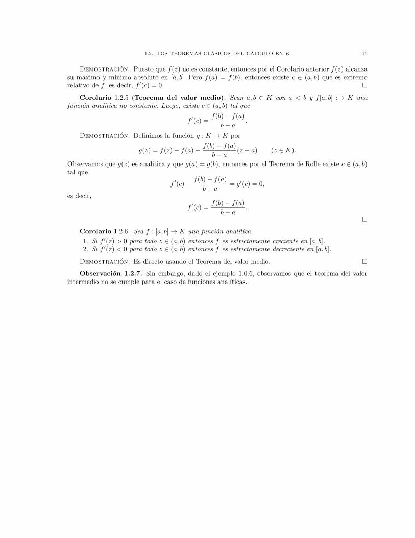
Demostracion. Puesto que f(z) no es constante, entonces por el Corolario anterior f(z) alcanzasu maximo y mınimo absoluto en [a, b]. Pero f(a) = f(b), entonces existe c ∈ (a, b) que es extremorelativo de f , es decir, f ′(c) = 0. �
Corolario 1.2.5 (Teorema del valor medio). Sean a, b ∈ K con a < b y f [a, b] :→ K unafuncion analıtica no constante. Luego, existe c ∈ (a, b) tal que
f ′(c) =f(b)− f(a)
b− a .
Demostracion. Definimos la funcion g : K → K por
g(z) = f(z)− f(a)− f(b)− f(a)
b− a (z − a) (z ∈ K).
Observamos que g(z) es analıtica y que g(a) = g(b), entonces por el Teorema de Rolle existe c ∈ (a, b)tal que
f ′(c)− f(b)− f(a)
b− a = g′(c) = 0,
es decir,
f ′(c) =f(b)− f(a)
b− a .
�Corolario 1.2.6. Sea f : [a, b]→ K una funcion analıtica.
1. Si f ′(z) > 0 para todo z ∈ (a, b) entonces f es estrictamente creciente en [a, b].2. Si f ′(z) < 0 para todo z ∈ (a, b) entonces f es estrictamente decreciente en [a, b].
Demostracion. Es directo usando el Teorema del valor medio. �Observacion 1.2.7. Sin embargo, dado el ejemplo 1.0.6, observamos que el teorema del valor
intermedio no se cumple para el caso de funciones analıticas.
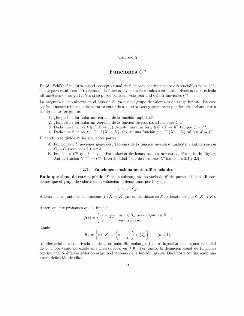
Capıtulo 2
Funciones Cn
En [3], Schikhof muestra que el concepto usual de funciones continuamente diferenciables no es sufi-ciente para establecer el teorema de la funcion inversa o resultados sobre antiderivacion en el calculoultrametrico de rango 1. Pero si se puede construir esta teorıa al definir funciones Cn.
La pregunta quedo abierta en el caso de K, ya que su grupo de valores es de rango infinito. En estecapıtulo mostraremos que la teorıa se extiende a nuestro caso y permite responder afirmativamente alas siguientes preguntas:
1. ¿Es posible formular un teorema de la funcion implıcita?.2. ¿Es posible formular un teorema de la funcion inversa para funciones Cn?.3. Dada una funcion f ∈ C(X → K), ¿existe una funcion g ∈ C1(X → K) tal que g′ = f?.4. Dada una funcion f ∈ Cn−1(X → K), ¿existe una funcion g ∈ Cn(X → K) tal que g′ = f?.
El capıtulo se divide en las siguientes partes:
A. Funciones C1: nociones generales, Teorema de la funcion inversa e implıcita y antiderivacionC → C1(secciones 2.1 a 2.3).
B. Funciones Cn que incluyen: Formulacion de lemas basicos necesarios, Formula de Taylor,Antiderivacion Cn−1 → Cn, Invertibilidad local de funciones Cn(secciones 2.4 y 2.5).
2.1. Funciones continuamente diferenciables
En lo que sigue de este capıtulo, X es un subconjunto no vacıo de K sin puntos aislados. Recor-demos que el grupo de valores de la valuacion lo denotamos por Γ, y que
gn := v(Xn).
Ademas, el conjunto de las funciones f : X → K que son continuas en X lo denotamos por C(X → K).
Anteriormente probamos que la funcion
f(z) =
{z − 1
X2nsi z ∈ Bn para algun n ∈ N.
z en otro caso.,
donde
Bn =
{z ∈ K : v
(z − 1
Xn
)< g−1
2n
}(n > 1),
es diferenciable con derivada continua no nula. Sin embargo, f no es inyectiva en ninguna vecindadde 0, y por tanto no existe una inversa local en f(0). Por tanto, la definicion usual de funcionescontinuamente diferenciables no asegura el teorema de la funcion inversa. Daremos a continuacion unanueva definicion de ellas.
17

2.1. FUNCIONES CONTINUAMENTE DIFERENCIABLES 18
Para una funcion f : X → K, definimos la funcion Φ1f de dos variables como
Φ1f(x, y) =f(x)− f(y)
x− y (x, y ∈ X, x 6= y).
Definicion 2.1.1. Diremos que una funcion f es continuamente diferenciable en a ∈ X o C1
en a si
1. Es diferenciable en a.2. Si para todo ε ∈ Γ existe δ ∈ Γ tal que si v(x− a) < δ, v(y − a) < δ y x 6= y entonces
v (Φ1f(x, y)− f ′(a)) < ε.
f es continuamente diferenciable en X si lo es para cada a ∈ X. Diremos que f es C1 en Xo f ∈ C1(X → K).
En el caso del analisis real, como consecuencia del teorema del valor medio, esta definicion es equivalentea la definicion clasica.
Proposicion 2.1.2. Sea f : X → K. Las siguientes condiciones son equivalentes:
1. f es continuamente diferenciable en X.2. La funcion Φ1f puede extenderse de manera unica a una funcion continua Φ1f sobre X ×X.3. Existe una funcion continua R : X ×X → K tal que
f(x) = f(y) + (x− y)R(x, y) (x, y ∈ X).
Demostracion. 1 ⇒ 2. Podemos definir Φ1f(x, y) = Φ1f(x, y) si x 6= y y Φ1f(x, x) = f ′(x).Se puede verificar directamente que Φ1f es continua sobre X ×X. La continuidad de Φ1f verifica launicidad de esta funcion, y por tanto es la unica extension continua.2⇒ 3. Basta con considerar R(x, y) = Φ1f(x, y) con x, y ∈ X.3⇒ 1. Es directo por la continuidad de R(x, y) en X ×X. �
Podemos entonces establecer un teorema de funcion inversa en este marco, en forma similar al obtenidoen [3] para cuerpos con valuacion de rango 1. Sin embargo, nuestra demostracion difiere fundamental-mente de esta, ya que el cuerpo K no es henseliano.
Teorema 2.1.3 (Invertibilidad local para funciones C1). Sea f : X → K una funciondefinida en alguna vecindad de a ∈ X. Si f es C1 en a y f ′(a) 6= 0, entonces para algun r ∈ Γsuficientemente pequeno la restriccion f : Ba(r)→ Bf(a)(v(f(a))r) de f a Ba(r) es inyectiva y sobre.La inversa local g de f
g : Bf(a)(v(f(a))r)→ Ba(r)
es C1 en f(a) y g′(f(a)) = f ′(a)−1.
Demostracion. Como f es C1 en a, para alguna bola Ba(r) se tiene que
sup
{v
(f(x)− f(y)
x− y − f ′(a)
): x, y ∈ Ba(r), x 6= y
}< v(X−1
1 f ′(a)).
Claramente f es inyectiva en Ba(r) y que ademas f(Ba(r)) ⊆ Bf(a)(v(f ′(a))r). Por otro lado, seac ∈ Bf(a)(v(s)r) donde s = f ′(a), entonces debemos probar que la funcion x 7→ f(x) − c tiene

2.2. ANTIDERIVACION C → C1. 19
un cero en Ba(r). Definimos la funcion h por h(z) = z − s−1(f(z) − c) y claramente se tiene queh(Ba(r)) ⊆ Ba(r). Sea x, y ∈ Ba(r), entonces
v(h(x)− h(y)) = v(x− y − s−1(f(x)− f(y)))
= v(s−1(x− y)) v
(f(x)− f(y)
x− y − s)
< v(X−11 (x− y)).
Luego, |h(x)− h(y)| < |X−11 (x− y)| para todo x, y ∈ Ba(r), lo que implica que
φ(|h(x)− h(y)|) ≤ φ(|X−11 (x− y)|) ≤ φ(|X−1
1 |)φ(|x− y|)y por tanto d(h(x), h(y)) ≤ 1
2d(x, y). Puesto que las topologıas generadas por d, | | y v( ) son iguales,aplicamos el teorema del punto fijo de Banach a h y obtenemos que esta ultima funcion tiene un unicopunto fijo en Ba(r). Se concluye que f : Ba(r)→ Bf(a)(v(f(a))r) es sobre.
Utilizando la desigualdad triangular fuerte observamos que
v(f(x)− f(y)) = v(f ′(a))v(x− y).
Luego, la funcion g : Bf(a)(v(f(a))r)→ Ba(r) es un multiplo de una isometrıa y por tanto es continua.Sea z, t ∈ Bf(a)(v(f(a))r), entonces
Φ1g(z, t) = (Φ1f(g(z), g(t)))−1
y g′(f(a)) = lım(z,t)→(f(a),f(a))
Φ1g(z, t) = lım(u,v)→(a,a)
(Φ1f(u, v))−1 = f ′(a)−1 obteniendose la afirmacion.
�
2.2. Antiderivacion C → C1.
Recordemos que X es un subconjunto no vacıo de K sin puntos aislados. Probaremos que toda funcionf ∈ C(X → K) tiene una antiderivada F ∈ C1(X → K). Comenzamos con algunas definicionesprevias.
Recordemos que para g ∈ Γ y s ∈ Γ#,
g · s = supΓ#
{gr : r ∈ G, r ≤ s}.
Una aproximacion de la identidad sobre X es una sucesion σ0, σ1, σ2, . . . de aplicaciones X → Xtales que σ0 es constante, σm ◦ σn = σn ◦ σm = σn si m ≥ n, y tal que para todo n ∈ N, x, y ∈ X
v(x− y) < g−1n implica σn(x) = σn(y),
v(σn(x)− x) < gn.
Definicion 2.2.1. Sea σ0, σ1, σ2, . . . una aproximacion de la identidad sobre X. Para una funcioncontinua f : X → K definimos
(Pf)(x) :=
∞∑
n=0
f(xn)(xn+1 − xn)
donde xn = σn(x), x ∈ X y n ∈ N.
2.2. ANTIDERIVACION C → C1. 20
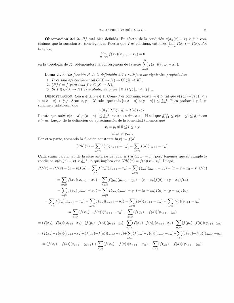
Observacion 2.2.2. Pf esta bien definida. En efecto, de la condicion v(σn(x) − x) < g−1n con-
cluimos que la sucesion xn converge a x. Puesto que f es continua, entonces lımn→∞
f(xn) = f(x). Por
lo tanto,
lımn→∞
f(xn)(xn+1 − xn) = 0
en la topologıa de K, obteniendose la convergencia de la serie
∞∑
n=0
f(xn)(xn+1 − xn).
Lema 2.2.3. La funcion P de la definicion 2.2.1 satisface las siguientes propiedades:
1. P es una aplicacion lineal C(X → K)→ C1(X → K),2. (Pf)′ = f para toda f ∈ C(X → K),3. Si f ∈ C(X → K) es acotada, entonces ‖Φ1(Pf)‖∞ ≤ ‖f‖∞.
Demostracion. Sea a ∈ X y ε ∈ Γ. Como f es continua, existe m ∈ N tal que v(f(x)−f(a)) < εsi v(x − a) < g−1
m . Sean x, y ∈ X tales que max{v(x − a), v(y − a)} ≤ g−1m . Para probar 1 y 2, es
suficiente establecer que
v(Φ1(Pf)(x, y)− f(a)) < ε.
Puesto que max{v(x − a), v(y − a)} ≤ g−1m , existe un unico s ∈ N tal que g−1
s+1 ≤ v(x − y) ≤ g−1s con
s ≥ m. Luego, de la definicion de aproximacion de la identidad tenemos que
xi = yi si 0 ≤ i ≤ s y,
xs+1 6= ys+1.
Por otra parte, tomando la funcion constante h(x) := f(a)
(Ph)(x) =∑
n∈Nh(x)(xn+1 − xn) =
∑
n∈Nf(a)(xn+1 − xn).
Cada suma parcial Sk de la serie anterior es igual a f(a)(xk+1 − x), pero tenemos que se cumple lacondicion v(σn(x)− x) < g−1
n , lo que implica que (Ph)(x) = f(a)(x− x0). Luego,
Pf(x)− Pf(y)− (x− y)f(a) =∑
n∈Nf(xn)(xn+1 − xn)−
∑
n∈Nf(yn)(yn+1 − yn)− (x− y + x0 − x0)f(a)
=∑
n∈Nf(xn)(xn+1 − xn)−
∑
n∈Nf(yn)(yn+1 − yn)− (x− x0)f(a) + (y − x0)f(a)
=∑
n∈Nf(xn)(xn+1 − xn)−
∑
n∈Nf(yn)(yn+1 − yn)− (x− x0)f(a) + (y − y0)f(a)
=∑
n∈Nf(xn)(xn+1 − xn)−
∑
n∈Nf(yn)(yn+1 − yn)−
∑
n∈Nf(a)(xn+1 − xn) +
∑
n∈Nf(a)(yn+1 − yn)
=∑
n∈N(f(xn)− f(a))(xn+1 − xn)−
∑
n∈N(f(yn)− f(a))(yn+1 − yn)
= (f(xs)−f(a))(xs+1−xs)−(f(ys)−f(a))(ys+1−ys)+∑
n>s
(f(xn)−f(a))(xn+1−xn)−∑
n>s
(f(yn)−f(a))(yn+1−yn)
= (f(xs)−f(a))(xs+1−xs)−(f(xs)−f(a))(ys+1−xs)+∑
n>s
(f(xn)−f(a))(xn+1−xn)−∑
n>s
(f(yn)−f(a))(yn+1−yn)
= (f(xs)− f(a))(xs+1 − ys+1) +∑
n>s
(f(xn)− f(a))(xn+1 − xn)−∑
n>s
(f(yn)− f(a))(yn+1 − yn).
2.3. EL TEOREMA DE LA FUNCION IMPLICITA 21
Observamos que,v(xn − a) ≤ max{v(xn − x), v(x− a)} ≤ gn−1
si n ≥ s, y por la continuidad de f tenemos que v(f(xn) − f(a)) ≤ ε si n ≥ s, de la misma forma seprueba que v(f(yn)− f(a)) ≤ ε si n ≥ s.Por otra parte,
v(xs+1 − ys+1) ≤ max{v(xs+1 − x), v(x− y), v(y − ys+1)} ≤ max{g−1s+1, v(x− y)} = v(x− y),
y para n > s tenemos que
v(xn+1 − xn) ≤ max{v(xn+1 − x), v(xn − x)} ≤ g−1n ≤ g−1
s+1 ≤ v(x− y).
Por lo tanto,v((Pf)(x)− (Pf)(y)− (x− y)f(a)) ≤ ε v(x− y),
lo que implica que Pf ∈ C1(X → K). Esto concluye la demostracion de las dos primeras afirmacionesdel lema.
Para demostrar la tercera, consideramos x, y ∈ X con x 6= y, entonces
(Pf)(x)− (Pf)(y) =∑
n∈Nf(xn)(xn+1 − xn)−
∑
n∈Nf(yn)(yn+1 − yn).
De forma similar a la parte anterior, se prueba que v(xn+1 − xn) y v(yn+1 − yn) estan acotadossuperiormente por v(x− y), lo que implica que
v((Pf)(x)− (Pf)(y)) ≤ v(x− y) · ‖f‖∞.�
Destacamos que como corolario se obtiene el siguiente teorema:
Teorema 2.2.4 (Antiderivacion C → C1). Toda funcion f ∈ C(X → K) tiene una antiderivadaF ∈ C1(X → K).
Demostracion. La demostracion es directa. �
2.3. El teorema de la funcion implıcita
Comenzamos esta seccion con el siguiente ejemplo:
Ejemplo 2.3.1. Recordemos que en el ejemplo 1.0.8, probamos que la funcion f : K → K definidapor
f(z) =
{z − 1
X2nsi z ∈ Bn para algun n ∈ N
z en otro caso,
donde
Bn =
{z ∈ K : v
(z − 1
Xn
)< g−1
2n
},
es una funcion diferenciable, con derivada no nula pero que no es inyectiva en ninguna vecindad delcero.
Consideramos ahora F : K ×K → K definida por F (x, y) = f(y)− x. Es inmediato que se cumplen:
1. F (0, 0) = 0,2. Fx(x, y) = −1 y Fy(x, y) = 1 son continuas en K ×K,3. Fy(0, 0) = 1 6= 0.
2.3. EL TEOREMA DE LA FUNCION IMPLICITA 22
Supongamos que existen vecindades U , V de 0, y una aplicacion h : U → V tales que
{(x, y) ∈ U × V : F (x, y) = 0} = {(x, h(x)) : x ∈ U}.Ahora al tomar, con n suficientemente grande, x = 1
Xn− 1
X2n∈ U , y1 = 1
Xn, e y2 = 1
Xn− 1
X2n∈ V ,
se tiene que
x =1
Xn− 1
X2n= f(y1) = f
(1
Xn
)= f
(1
Xn− 1
X2n
)= f(y2).
Entonces F (x, y1) = F (x, y2) = 0 lo que implica que la aplicacion h no es funcion. De este modo, elteorema de la funcion implıcita no se cumple en K en su forma clasica.
Las dificultades desaparecen si exigimos condiciones adicionales. Necesitaremos dos resultados previos.
Lema 2.3.2. Sea X ⊂ K sin puntos aislados y sea (fn)n una sucesion de funciones C1 en X.Supongamos que f(x) := lım
n→∞fn(x) existe puntualmente en X y que lım
n→∞Φ1fn existe uniformemente
en X ×X \∆. Entonces f ∈ C1(X → K) y lımn→∞
Φ1fn = Φ1f uniformemente en X ×X.
Demostracion. Sea a ∈ X, primero probaremos que f es C1 en a. Sea ε ∈ Γ y sean x, y ∈ Xtales que x 6= y. Observamos que
v(f ′n+1(a)− f ′n(a)) ≤ max
{v
(f ′n+1(a)− fn+1(x)− fn+1(y)
x− y
), v
(fn(x)− fn(y)
x− y − f ′n(a)
),
v
(fn+1(x)− fn+1(y)
x− y − fn(x)− fn(y)
x− y
)}.
Puesto que (Φ1fn)n converge uniformemente en X ×X \∆, existe n0 ∈ N tal que para todo n ≥ n0
supΓ#
{v
(fn+1(x)− fn+1(y)
x− y − fn(x)− fn(y)
x− y
): x, y ∈ X, x 6= y
}< ε.
Sea m ∈ N con m ≥ n0. Recordemos que fn ∈ C1(X → K) para todo n ∈ N, en particular para todon ≥ n0. Entonces existe una vecindad Vm de a tal que para todo x, y ∈ Vm
supΓ#
{v
(f ′m+1(a)− fm+1(x)− fm+1(y)
x− y
), v
(fm(x)− fm(y)
x− y − f ′m(a)
)}< ε.
Luego, si x, y ∈ Vm con x 6= y entonces
v(f ′m+1(a)− f ′m(a)) ≤ max
{v
(f ′m+1(a)− fm+1(x)− fm+1(y)
x− y
), v
(fm(x)− fm(y)
x− y − f ′m(a)
),
v
(fm+1(x)− fm+1(y)
x− y − fm(x)− fm(y)
x− y
)}
< ε.
Como n ≥ n0 es arbitrario, obtenemos que (f ′n(a))n es una sucesion de Cauchy en K. Pero la existenciade n0 es independiente de a ∈ X, pues solo depende de la convergencia uniforme de (Φ1fn)n enX ×X \∆. Por lo tanto, (f ′n)n converge uniformemente en K.
Sea ma = lımn→∞
f ′n(a), si x, y ∈ Vm con x 6= y entonces
v
(f(x)− f(y)
x− y −ma
)≤ max
{v
(f(x)− f(y)
x− y − fn(x)− fn(y)
x− y
), v (f ′n(a)−ma) ,
2.3. EL TEOREMA DE LA FUNCION IMPLICITA 23
v
(fn(x)− fn(y)
x− y − f ′n(a)
)}.
Por argumentos similares a los utilizados en la parte anterior, se prueba que f es C1 en a y f ′(a) = ma.
Para la segunda afirmacion, solo basta verificar que la sucesion (f ′n)n converge uniformemente enX, pero esto ultimo esta dado en la primera parte de la demostracion. Por lo tanto, tenemos quelımn→∞
Φ1fn = Φ1f uniformemente en X ×X. �
El lema anterior nos permite construir un espacio metrico completo.
Sea f ∈ C1(X → K) y supongamos que ‖f‖∞ y ‖Φ1f‖∞ existen. Definimos ‖f‖1 = max{‖f‖∞, ‖Φ1f‖∞}y
BC1(X → K) := {f ∈ C1(X → K) : ‖f‖1 existe}.Este es un espacio normado sobre K (en el sentido de [5]) y ‖f‖1 es no arquimediana con valores enΓ#. La topologıa dada por la norma se denotara por τ(B), y sus entornos basales tienen la forma
Af (q−) = {g ∈ BC1(X → K) : ‖g − f‖1 < q}.para cada f ∈ BC1(X → K) y q ∈ Γ#.
Por otra parte definimos una (ultra)metrica d1 en BC1(X → K) utilizando para ello la ultrametricad : K → R+ (ver Preliminares). Recordamos que el conjunto de valores de d es discreto, por lo quehablamos de maximos en vez de supremos. En forma precisa, tenemos:
d1 : BC1(X → K)×BC1(X → K)→ R+
d1(f, g) := max
{maxx∈X{d(f(x), g(x))}, max
(x,y)∈X×X\∆{d(Φ1f(x, y),Φ1g(x, y))}
},
Es una verificacion directa que d1 es una ultrametrica en BC1(X → K); por tanto induce una topologıaen este conjunto.
Sea Bf (n) = {g ∈ BC1(X → K) : maxx∈X d(f(x), g(x)) < 12n } y BΦ1f (n) = {g ∈ BC1(X → K) :
maxx∈X d(Φ1f,Φ1g) < 12n } y recordemos que para todo a ∈ K y n ∈ N \ {0}
{z ∈ K : d(z, a) <1
2n} ⊂ {z ∈ K : v(z − a) < g−1
n } ⊂ {z ∈ K : d(z, a) <1
2n−1}.
De aquı se derivan las siguientes inclusiones para todo n ∈ N \ {0}Bf (n) ⊂ {g ∈ BC1(X → K) : ‖f − g‖∞ < g−1
n } ⊂ Bf (n− 1),
BΦ1f (n) ⊂ {g ∈ BC1(X → K) : ‖Φ1f − Φ1g‖∞ < g−1n } ⊂ BΦ1f (n− 1).
Luego para todo f, g en BC1(X → K), si d1(f, g) < 12n entonces ‖f − g‖1 < g−1
n lo que a su vez
implica que d1(f, g) < 12n−1 .
Por lo tanto, las topologıas inducidas por ‖ ‖1 y d1 en BC1(X → K) son iguales.
La ultrametrica d1 genera una uniformidad en BC1(X → K) de la siguiente manera: para cada s ∈ R+
consideramos los conjuntos
Vs = {(f, g) : f, g ∈ BC1(X → K), d1(f, g) < s}.Se puede probar directamente que el conjunto {Vs : s ∈ R+} es una base para una uniformidad Ud1en BC1(X → K).

2.3. EL TEOREMA DE LA FUNCION IMPLICITA 24
Por otra parte, para cada r ∈ Γ# consideramos los conjuntos
Sr = {(f, g) : f, g ∈ BC1(X → K), ‖f − g‖1 < r}.Se satisface las siguientes propiedades:
1. (Sr)−1 = {(g, f) : (f, g) ∈ Sr} = Sr,
2. Sr ∩ St = Sk, donde k = mın{s, t},3. Sr ◦ Sr = {(f, h) : existe g ∈ BC1(X → K) tal que (f, g), (g, h) ∈ Sr} = Sr.
Por lo tanto, {Sr : r ∈ Γ#} es una base para una uniformidad U‖ ‖1 . Dada la relacion que existe entrelas bolas abierta generadas por d1 y ‖ ‖1, se tiene que V 1
2n⊂ Sg−1
n⊂ V 1
2n−1. Entonces, los conjuntos
{Vs : s ∈ R+} y {Sr : r ∈ Γ#} son bases para una misma uniformidad, es decir, Ud1 = U‖ ‖1 . Estauniformidad en comun la denotamos por U .
El espacio uniforme (BC1(X → K),U) es ultrametrizable, entonces este es completo si y solo si todasucesion de Cauchy converge en BC1(X → K). Por lo tanto, si B es una base de U , entonces unasucesion fn es de Cauchy si y solo si para todo miembro U de B existe n0 ∈ N tal que si m,n ≥ n0
implica (am, an) ∈ U . Luego, las siguientes afirmaciones son equivalentes:
1. (fn)n∈N es una sucesion de Cauchy en (BC1(X → K),U).2. Para todo ε > 0 existe n0 ∈ N tal que si m,n ≥ n0 entonces d1(am, an) < ε.3. Para todo ε ∈ Γ# existe n1 ∈ N tal que si m,n ≥ n1 entonces ‖am − an‖1 < ε.
Lema 2.3.3. (BC1(X → K), d1) es un espacio metrico completo.
Demostracion. Sea (fn)n una sucesion de Cauchy en (BC1(X → K), d1).
Dada la relacion entre ‖ ‖1 y d1 establecida anteriormente, basta probar que (fn)n converge en(BC1(X → K), ‖ ‖1).
Sea ε ∈ Γ#, entonces existe m ∈ N tal que para todo k, n ≥ m,
max{‖Φ1fk − Φ1fn‖∞, ‖fk − fn‖∞} < ε.
Para cada x ∈ K observamos que v(fk(x)− fn(x)) ≤ ‖fk− fn‖∞ < ε, entonces cada sucesion (fn(x))nes de Cauchy y por lo tanto converge en K.
Definimos la funcion f : X → K como f(x) = lımn→∞
fn(x). Probaremos que fn converge uniformemente
a f en X. Puesto que,
max{‖Φ1fk − Φ1fn‖∞, ‖fk − fn‖∞} < ε (k, n ≥ m),
entonces para todo x ∈ Kv(fk(x)− fn(x)) < ε (k, n ≥ m).
Si k →∞ en el lado izquierdo de la expresion anterior, para todo x ∈ K se tiene que
v(f(x)− fn(x)) < ε (n ≥ m).
Por lo tanto, ‖f − fn‖∞ < ε para todo n ≥ m.
Ahora, si (x, y) ∈ X ×X \∆,
Φ1f(x, y) =f(x)− f(y)
x− y = lımn→∞
fn(x)− fn(y)
x− y = lımn→∞
Φ1fn(x, y).
Pero, para todo n, k ≥ msupΓ#
{v (Φ1fk(x, y)− Φ1fn(x, y)) : x, y ∈ X, x 6= y} ≤ ‖fk − fn‖1 < ε.

2.3. EL TEOREMA DE LA FUNCION IMPLICITA 25
Entonces, procediendo de la misma forma que en el caso de f , si k →∞ tenemos que ‖Φ1f−Φ1fn‖∞ < εpara todo n ≥ m en X ×X \∆.
Luego, f(x) = lımn→∞
fn(x) uniformemente en X y lımn→∞
Φ1fn(x, y) existe uniformemente en X ×X \∆,
por el Lema anterior se obtiene que f ∈ C1(X → K) y lımn→∞
Φ1fn = Φ1f uniformemente en X ×X.
Por lo tanto, fn converge a f en (BC1(X →,K), ‖ ‖1).
Por otro lado, considerando m ∈ N de la parte anterior,
v(f(x)) = v(fm(x) + f(x)− fm(x))
≤ max{v(fm(x)), v(f(x)− fm(x)))}≤ max{v(fm(x)), ‖f − fm‖∞}≤ max{‖fm‖∞, ε}.
Puesto que fm ∈ BC1(X → K), tenemos que ‖f‖∞ <∞. En forma similar se prueba que ‖Φ1f‖∞ <∞. Por lo tanto, f ∈ BC1(X → K). �
Corolario 2.3.4. Si C es un subconjunto cerrado de K, entonces (BC1(X → C), d1) es un espaciometrico completo.
Demostracion. Sea (fn)n una sucesion de Cauchy en BC1(X → C). Por la proposicion anterior,BC1(X → K) es completo con la metrica d1. Observamos que BC1(X → C) ⊂ BC1(X → K),entonces existe una funcion f ∈ BC1(X → K) tal que fn converge a f en (BC1(X → K), d1).Debemos probar que f ∈ BC1(X → C).
Puesto que f ∈ BC1(X → K), tenemos que f es C1 en X y ‖f‖1 <∞, entonces solo debemos verificarque f(X) ⊂ C. Pero, (fn(x))n es una sucesion en C para cada x ∈ Bx0(r), y como C es cerrado en K,se tiene que f(x) = lım
n→∞fn(x) ∈ C. �
Enunciamos ahora el teorema principal de esta seccion.
Teorema 2.3.5 (Teorema de la Funcion Implıcita). Sea F : K2 → K una funcion continuay (x0, y0) ∈ K2. Supongamos que
1. F (x0, y0) = 0,2. la funcion G definida por
G(x, y, y′) =F (x, y)− F (x, y′)
y − y′
se extiende a una funcion continua G : K3 → K,3. la funcion H definida por
H(x, x′, y) =F (x, y)− F (x′, y)
x− x′
se extiende a una funcion continua H : K3 → K,4. Fy(x0, y0) 6= 0.
Entonces existen vecindades U y V de x0 e y0 respectivamente, y una unica funcion ψ ∈ C1(U → V )tal que F (x, ψ(x)) = 0 para todo x ∈ U .

2.3. EL TEOREMA DE LA FUNCION IMPLICITA 26
Demostracion. La prueba del teorema tiene tres partes. En la primera se escoge apropiadamentevalores de r y δ para que Bx0(r) sea eventualmente el entorno U y By0(δ) el entorno V . Luego en elespacio metrico completo (BC1(Bx0
(r)→ By0(δ)), d1) se elige una funcion h, se prueba que esta biendefinida, y que es una contraccion. El teorema del punto fijo de Banach permite completar la prueba.
Sea s = Fy(x0, y0). Observamos que el lımite de G(x0, y0, y) cuando y → y0 es G(x0, y0, y0) =Fy(x0, y0).
Puesto que G es continua en K3 y Fy(x0, y0) 6= 0, existe δ ∈ Γ tal que si x ∈ Bx0(δ), y, y′ ∈ By0(δ)
con y 6= y′, entonces
v
(F (x, y)− F (x, y′)
y − y′ − s)< g−1
1 v(s).
Por la desigualdad triangular fuerte observamos que
v(F (x, y)− F (x, y′)) = v(s)v(y − y′)
si y, y′ ∈ By0(δ), x ∈ Bx0(δ). Del mismo modo, usando la continuidad de H en K3, se puede probar
que existe δ1 ∈ Γ tal que si x, x′ ∈ Bx0(δ1), y ∈ By0(δ1) entonces
v(F (x, y)− F (x′, y)) = v(s)v(x− x′).
Por otro lado, F (x, y) es continua en (x0, y0) y F (x0, y0) = 0, entonces existe δ2 ∈ Γ tal quev(F (x, y0)) ≤ s · δ si x ∈ Bx0(δ2).
Sea r = mın{δ, δ1, δ2} y consideramos el conjunto
BC1(Bx0(r)→ By0(δ)) := {f ∈ C1(Bx0
(r)→ By0(δ)) : max{‖f‖∞, ‖Φ1f‖∞} <∞}.
Recordemos que By0(δ) es un subconjunto cerrado de K, entonces por el corolario 2.3.4 se tiene que(BC1(Bx0(r)→ By0(δ)), d1) es un espacio metrico completo.
Para f ∈ BC1(Bx0(r)→ By0(δ)), definimos la funcion
h : BC1(Bx0(r)→ By0(δ))→ BC1(Bx0
(r)→ By0(δ))
como
(h(f))(x) := f(x)− s−1F (x, f(x)).
Probaremos que h esta bien definida. Si x ∈ Bx0(r), entonces
v((h(f))(x)− y0) = v(f(x)− s−1F (x, f(x))− s−1F (x, y0) + s−1F (x, y0)− y0)
≤ max{v(f(x)− y0), v(s−1)v(F (x, f(x))− F (x, y0)), v(s−1F (x, y0))}.
Puesto que v(F (x, y)− F (x, y′)) = v(s)v(y − y′) si y, y′ ∈ By0(δ), x ∈ Bx0(r), tenemos que
v(s−1)v(F (x, f(x))− F (x, y0)) = v(f(x)− y0).
Por otra parte, v(F (x, y0)) ≤ v(s) δ si v(x− x0) ≤ r, lo que implica que v((h(f))(x)− y0) ≤ δ. Luego,(h(f))(x) ∈ By0(δ).

2.3. EL TEOREMA DE LA FUNCION IMPLICITA 27
Sean x, y ∈ Bx0(δ) con x 6= y, entonces
Φ1(h(f))(x, y) =f(x)− s−1F (x, f(x))− f(y) + s−1F (y, f(y))
x− y
= Φ1f(x, y)− s−1
(F (x, f(x))− F (x, f(y)) + F (x, f(y))− F (y, f(y))
x− y
)
= Φ1f(x, y)− s−1
(F (x, f(x))− F (x, f(y))
x− y +F (x, f(y))− F (y, f(y))
x− y
).
Como f ∈ BC1(Bx0(r)→ By0(δ)) y G,H son continuas en K3, tenemos que h(f) es C1 en Bx0(r).
Recordemos que si x, y ∈ Bx0(r) y f(x), f(y) ∈ By0(δ), entonces v(F (x, f(y))−F (y, f(y))) = v(s)v(x−
y) y v(F (x, f(x)))− F (x, f(y))) = v(s)v(f(x)− f(y)). Luego, de la expresion
Φ1(h(f))(x, y) = Φ1f(x, y)− s−1
(F (x, f(x))− F (x, f(y))
x− y +F (x, f(y))− F (y, f(y))
x− y
)
podemos concluir que
v(Φ1(h(f))(x, y)) ≤ max{v(Φ1f(x, y)), v(s−1)v(sΦ1f(x, y)), v(s)−1v(x− y)−1v(s)v(x− y)
}
≤ max{v(Φ1f(x, y)), 1}.Por lo tanto, ‖Φ1(h(f))‖∞ < ∞ y h(f) ∈ BC1(Bx0
(δ) → By0(r)), lo que implica que h esta biendefinida.
Finalmente, probaremos que
h : (BC1(Bx0(r)→ By0(δ)), d1)→ (BC1(Bx0(r)→ By0(δ)), d1)
es una contraccion, y por tanto tiene un punto fijo.
Sean f, g ∈ BC1(Bx0(r)→ By0(δ)), luego para todo x ∈ Bx0
(r) con f(x) 6= g(x)
v((h(f))(x)− (h(g))(x)) = v((f(x)− s−1F (x, f(x)))− (g(x)− s−1F (x, g(x))))
= v((f(x)− g(x))− s−1(F (x, f(x))− F (x, g(x))))
= v(s−1(f(x)− g(x)))v
(s− F (x, f(x))− F (x, g(x))
f(x)− g(x)
).
Puesto que para cada x ∈ Bx0(r) se tiene que f(x), g(x) ∈ By0(δ), y de la condicion
v
(F (x, y)− F (x, y′)
y − y′ − s)< g−1
1 v(s),
observamos que
v
(F (x, f(x))− F (x, g(x))
f(x)− g(x)− s)< g−1
1 v(s).
Luego, si x ∈ Bx0(r) tal que f(x) 6= g(x),
v((h(f))(x)− (h(g))(x)) = v((f(x)− s−1F (x, f(x)))− (g(x)− s−1F (x, g(x))))
≤ v(F (x, f(x))− F (x, g(x))
f(x)− g(x)− s)v(s−1)v(f(x)− g(x))
< g−11 v(f(x)− g(x)).

2.4. FUNCIONES Cn 28
Del mismo modo que en la demostracion del Teorema de la funcion inversa para funciones C1,
d((h(f))(x), (h(g))(x)) ≤ 1
2d(f(x), g(x))) (x ∈ Bx0
(δ), f(x) 6= g(x)).
Si f(x) = g(x) para algun x ∈ Bx0(r), entonces (h(f))(x) = (h(g))(x) y se cumple la desigualdadanterior. Por lo tanto, para todo x ∈ Bx0(r) se tiene que
d((h(f))(x), (h(g))(x)) ≤ 1
2d(f(x), g(x))) ≤ 1
2d1(f, g).
Siguiendo el mismo tipo de argumento se prueba que
d(Φ1(h(f))(x, y),Φ1(h(g))(x, y)) ≤ 1
2d(Φ1f(x, y),Φ1g(x, y)) ≤ 1
2d1(f, g) (x, y ∈ Bx0
(r)).
Por lo tanto, h es una contraccion. Por el Teorema del punto fijo de Banach existe un unica funcion
ψ ∈ BC1(Bx0(r)→ By0(δ))
tal que (h(ψ))(x) = ψ(x). Pero (h(ψ))(x) = ψ(x)− s−1F (x, ψ(x)), es decir, F (x, ψ(x)) = 0 para todox ∈ Bx0
(r).�
2.4. Funciones Cn
Al igual que en el caso de las funciones continuamente diferenciales, introduciremos una nueva nocion defuncion Cn. Por tanto daremos nuevas definiciones siguiendo las lıneas de [3], donde se construyo estateorıa para cuerpos con valuaciones de rango 1.
Definicion 2.4.1. Para cada n ∈ N, sea
∇nX := {(x1, x2, . . . , xn) ∈ Xn : si i 6= j entonces xi 6= xj}.El n-esimo cuociente de diferencias Φnf : ∇n+1X → K de una funcion f : X → K se define inducti-vamente como Φ0f = f y
Φnf(x1, x2, . . . , xn+1) =Φn−1f(x1, x3, . . . , xn+1)− Φn−1f(x2, x3, . . . , xn+1)
x1 − x2,
donde n ∈ N \ {0} y (x1, x2, . . . , xn+1) ∈ ∇n+1X.
Para cada n ≥ 1 consideraremos Xn con la topologıa producto con respecto a la topologıa relativa aX. Diremos que f es una funcion Cn en X si Φnf puede extenderse a una funcion continua
Φnf : Xn+1 → K.
El conjunto de las funciones Cn en X sera denotado por Cn(X → K). Definimos ademas
C∞(X → K) :=⋂
n∈NCn(X → K),
y sus elementos se llamaran funciones C∞.
En el siguiente lema estableceremos propiedades de Φnf .
Lema 2.4.2. Sean f, g : X → K y λ, µ ∈ K y n ∈ N \ {0}. Luego, se tienen las siguientesafirmaciones:
1. Si (x, y, z, x1, . . . , xn−1) ∈ ∇n+2X entonces
(x− y)Φnf(x, y, x1, . . . , xn−1) + (y − z)Φnf(y, z, x1, . . . , xn−1) = (x− z)Φnf(x, z, x1, . . . , xn−1).
2.4. FUNCIONES Cn 29
2. Φnf es una funcion simetrica de sus n+1 variables, es decir, es invariante bajo permutacionesσ ∈ Sn+1.
3. Si (x1, . . . , xn, a1, . . . , an) ∈ ∇2nX, entonces
Φn−1f(x1, . . . , xn)− Φn−1f(a1, . . . , an) =
n∑
j=1
(xj − aj)Φnf(a1, . . . , aj , xj , . . . , xn).
4. Φn(λf + µg) = λΦnf + µΦng.5. Si (x1, . . . , xn+1) ∈ ∇n+1X, entonces
Φn(fg) =
n∑
j=0
Φjf(x1, . . . , xj+1)Φn−jg(xj+1, . . . , xn).
6. Si f(x) 6= 0 para todo x ∈ X, g = 1f , (x1, . . . , xn+1) ∈ ∇n+1X, entonces
Φng = −f(x1)−1n∑
j=1
Φjf(x1, . . . , xj+1)Φn−jg(xj+1, . . . , xn+1).
Demostracion. 1. De la definicion de Φnf , tenemos que
(x− y)Φnf(x, y, x1, . . . , xn−1) + (y − z)Φnf(y, z, x1, . . . , xn−1)
= (Φn−1f(x, x1, . . . , xn−1)−Φn−1f(y, x1, . . . , xn−1))+(Φn−1f(y, x1, . . . , xn−1)−Φn−1f(z, x1, . . . , xn−1))
= (Φn−1f(x, x1, . . . , xn−1)− Φn−1f(z, x1, . . . , xn−1)) = (x− z)Φnf(x, z, x1, . . . , xn−1).
2. Procederemos por induccion sobre n ≥ 2. El caso n = 2 esta dado por la definicion de Φ1f .Por otra parte, por 1 se prueba directamente que
Φnf(x1, x2, x3, . . . , xn+1) = Φnf(x3, x2, x1, . . . , xn+1).
La hipotesis de induccion nos dice que Φn−1f es simetrica, lo que implica que Φnf invariantebajo las permutaciones de x2, x3 y permutaciones de x1, x4, . . . , xn+1. Por lo tanto, podemosdeducir que es invariante bajo la permutacion xσ(i) = xi+1 si 1 ≤ i ≤ n y xσ(n+1) = x1. Perola hipotesis de induccion tambien implica que Φnf es invariante por permutaciones de x1, x2.Por lo tanto, Φnf es invariante bajo la transposicion (1 2) y el ciclo (1 2 · · · n + 1) que songeneradores del grupo Sn.
3. Por la definicion de Φnf ,
Φn−1f(x1, . . . , xn)− Φn−1f(a1, . . . , an) = (Φn−1f(x1, . . . , xn)− Φn−1f(a1, x2, . . . , xn))
+(Φn−1f(a1, x2, . . . , xn)−Φn−1f(a1, a2, x3, . . . , xn))+. . .+(Φn−1f(a1, . . . , an−1, xn)−Φn−1f(a1, . . . , an))
= (Φn−1f(x1, . . . , xn)− Φn−1f(a1, x2, . . . , xn))
+
n−1∑
j=1
(Φn−1f(a1, . . . , aj , xj+1, . . . , xn)− Φn−1f(a1, . . . , aj+1, xj+2, . . . , xn))
= −(a1 − x1)Φnf(a1, x1, . . . , xn) + (xn − an)
n∑
j=2
Φnf(a1, . . . , aj , xj , . . . , xn).
4. Es directo usando la definicion de Φnf .

2.4. FUNCIONES Cn 30
5. Sea (x1, x2, . . . , xn+1) ∈ ∇n+1X. El caso n = 1 es trivial. Supongamos que es cierto para n−1con n > 1. La definicion de Φn(fg) nos dice que
Φn(fg)(x1, . . . , xn+1) =(Φn−1(fg)(x1, x3, . . . , xn+1)− Φn−1(fg)(x2, x3, . . . , xn+1)
x1 − x2.
Consideremos a1 = x1, b1 = x2 y ai = bi = xi+1 para i ≥ 2. Por hipotesis de induccion
Φn(fg)(x1, . . . , xn+1) =
n−1∑
j=0
Φjf(a1, . . . , aj+1)Φn−1−jg(aj+1, . . . , an)
a1 − b1
−
n−1∑
j=0
Φjf(b1, . . . , bj+1)Φn−1−jg(bj+1, . . . , bn)
a1 − b1.
Haciendo calculos elementales, obtenemos
Φn(fg)(x1, . . . , xn+1) =Φ0f(x1)Φn−1g(x1, x3, . . . , xn+1)− Φ0f(x2)Φn−1g(x2, . . . , xn+1)
x1 − x2
+
n∑
j=2
Φjf(x1, x2, . . . , xj+1)Φn−jg(xj+1, . . . , xn+1)
=Φ0f(x1)Φn−1g(x1, x3, . . . , xn+1)
x1 − x2+
(Φ0f(x1)− Φ0f(x2))Φn−1g(x2, . . . , xn+1)
x1 − x2
−Φ0f(x1))Φn−1g(x2, . . . , xn+1)
x1 − x2+
n∑
j=2
Φjf(x1, x2, . . . , xj+1)Φn−jg(xj+1, . . . , xn+1)
=Φ0f(x1)(Φn−1g(x1, x3, . . . , xn+1)− Φn−1g(x2, . . . , xn+1))
x1 − x2+
n∑
j=1
Φjf(x1, x2, . . . , xj+1)Φn−jg(xj+1, . . . , xn+1)
= Φ0f(x1)Φng(x1, x2, . . . , xn+1) +
n∑
j=1
Φjf(x1, x2, . . . , xj+1)Φn−jg(xj+1, . . . , xn+1).
6. Si (fg) = 1, entonces Φn(fg) = 0 para todo n ∈ N \ {0}. Utilizando la parte anterior
0 =
n∑
j=0
Φjf(x1, . . . , xj)Φn−jg(xj+1, . . . , xn)
= f(x1)Φng(x1, . . . , xn+1) +
n∑
j=0
Φjf(x1, . . . , xj)Φn−jg(xj+1, . . . , xn),
obteniendo la afirmacion.�
Corolario 2.4.3. Cn(X → K) ⊂ Cn−1(X → K) para todo n ≥ 1.

2.4. FUNCIONES Cn 31
Demostracion. Sea f ∈ Cn(X → K). Si (x1, . . . , xn, a1, . . . , an) ∈ ∇2nX, por 3 del lema anterior
Φn−1f(x1, . . . , xn)− Φn−1f(a1, . . . , an) =
n∑
j=1
(xj − aj)Φnf(a1, . . . , aj , xj , . . . , xn).
Fijamos a1, a2, . . . , an distintos entre sı. Puesto que f ∈ Cn(X → K), podemos extender continuamenteel lado derecho de la expresion anterior para todo (x1, . . . , xn) ∈ X y por definicion f ∈ Cn−1(X →K). �
Lema 2.4.4. Sea f ∈ Cn−1(X → K) para algun n ≥ 1. Luego Φnf puede extenderse a una funcioncontinua Φ∗nf en Xn+1 \∆, donde la diagonal ∆ es el conjunto
∆ := {(x, x, x, . . . , x) : x ∈ X}.Demostracion. Para 1 ≤ i, j ≤ n+ 1, i 6= j definimos los conjuntos
Ui,j = {(x1, . . . , xn+1 : xi 6= xj)}.Sean xi, xj ∈ X tales que xi 6= xj . Tenemos que la topologıa en K es Haussdorf, por lo tanto ladiagonal en X es cerrada en X ×X. Entonces existe δi,j ∈ G tal que el conjunto
{(x, y) ∈ X ×X : max{v(x− xi), v(y − xj)} < δi,j}esta contenido propiamente en X ×X \∆.
Sea δ = mın{δi,j : 1 ≤ i, j ≤ n+ 1}, entonces
{(a1, . . . , an+1) ∈ Xn+1 : max{v(ak − xk) : 1 ≤ k ≤ n+ 1} < δ} ⊂ Ui,j ,y por tanto Ui,j es abierto en Xn+1. Ademas,
⋃
i,j
Ui,j = Xn+1 \∆.
Definimos hi,j : Ui,j → K por
hi,j(x1, . . . , xn+1) := (xi−xj)−1(Φn−1f(x1, . . . , xj−1, xj+1, . . . , xn+1)−Φn−1f(x1, . . . , xi−1, xi+1, . . . , xn+1)).
Puesto que f ∈ Cn−1(X → K), hi,j es una funcion continua sobre Ui,j y que extiende a Φn−1f . Luego,definimos
Φ∗nf(x1, x2, . . . , xn+1) := hi,j(x1, x2, . . . , xn+1)
si (x1, x2, . . . , xn+1) ∈ Ui,j , y
Φ∗nf(x1, x2, . . . , xn+1) = Φnf(x1, x2, . . . , xn+1)
si (x1, x2, . . . , xn+1)∇n+1X. La buena definicion y la continuidad esta dada porque los abiertos Ui,json disjuntos entre sı y por la continuidad de hi,j sobre cada Ui,j . �
Definicion 2.4.5. Sea n ∈ N. Una funcion f : X → K se dice que es Cn en un punto a ∈ X,si el siguiente lımite
lımu→a, u∈∇n+1X
Φnf(u) (a = (a, . . . , a) ∈ Xn+1)
existe.
Teorema 2.4.6. Una funcion es Cn en X si y solo si f es Cn en cada a ∈ X.

2.4. FUNCIONES Cn 32
Demostracion. Si f ∈ Cn(X → K), claramente f lo es en cada a ∈ X.Por otro lado, supongamos que f es Cn en cada a ∈ X. Probaremos por induccion sobre n ≥ 1 quef ∈ Cn(X → K). El caso n = 1 esta dado por la Proposicion 2.1.2. Ahora supongamos que es ciertopara n− 1 si n > 1.
Sea a ∈ X. Por la hipotesis de induccion se tiene que f es Cn−1 en X. Luego, por el lema 2.4.4, Φnfse puede extender a una funcion continua Φ∗nf en Xn+1 \∆.
Definimos la funcion Φnf : Xn+1 → K como sigue:
Φnf(a1, . . . , an+1) =
Φ∗nf(a1, . . . , an+1) si (a1, . . . , an+1) ∈ Xn+1 \∆
lımu→a, u∈∇n+1X
Φnf(u) si a = (a1, . . . , an+1) ∈ ∆.
Para probar la continuidad de Φnf en Xn+1, solo basta probar que es continua en ∆.
Sea ε ∈ G y supongamos que a = (a, a, . . . , a). Consideramos l := lımu→a, u∈∇n+1X
Φnf(u) ∈ K, entonces
existe δ ∈ G tal que si (u1, . . . , un+1) ∈ ∇n+1X y max{v(ui − ai)} < δ implica
v(Φnf(u1, . . . , un+1)− l) < ε.
Probaremos que para todo (y1, . . . , yn+1) ∈ Xn+1 tal que max{v(yi−ai)} < δ se tiene que v(Φnf(y1, . . . , yn+1)−l) < ε.
Supongamos que existe (y1, . . . , yn+1) ∈ Xn+1 tal que max{v(yi − ai)} < δ y
v(Φnf(y1, . . . , yn+1)− l) > ε.
Puesto que l = lımu→a, u∈∇n+1X
Φnf(u) existe, se tiene que (y1, . . . , yn+1) ∈ Xn+1 \ (∇n+1X ∪∆), o bien,
(y1, . . . , yn+1) ∈ ∆. Si (y1, . . . , yn+1) ∈ Xn+1 \ (∇n+1X ∪∆), entonces por la continuidad de Φ∗nf enXn+1 \∆ existe δ1 ∈ G tal que si (x1, . . . , xn+1) ∈ Xn+1 \∆ y max{v(xi − yi)} < δ1 implica
(Φ∗nf(x1, . . . , xn+1)− Φ∗nf(y1, . . . , yn+1)) < ε.
Sin perder generalidad supongamos que δ1 < δ.
Luego, si max{v(xi − yi)} < δ1 y (x1, . . . , xn+1) ∈ ∇n+1X
v(xi − ai) ≤ max{v(xi − yi), v(yi − ai)} < δ,
lo que implica quev(Φnf(x1, . . . , xn+1)− l) < ε.
Por otra parte,
v(Φnf(x1, . . . , xn+1)− l) ≤ max{v(Φnf(x1, . . . , xn+1)−Φnf(y1, . . . , yn+1)), v(Φnf(y1, . . . , yn+1)− l)}.Puesto que v(Φnf(y1, . . . , yn+1) − l) > ε y v(Φnf(x1, . . . , xn+1) − Φnf(y1, . . . , yn+1)) < δ, por ladesigualdad triangular fuerte
v(Φnf(x1, . . . , xn+1)− l) = ε,
lo que contradice que v(Φnf(x1, . . . , xn+1)−l) < ε. Por lo tanto, si (y1, . . . , yn+1) ∈ Xn+1\(∇n+1X∪∆)y max{v(yi − ai)} < δ entonces v(Φnf(y1, . . . , yn+1)− l) < ε.
Utilizando el mismo tipo de argumento se puede probar que si (y1, . . . , yn−1) ∈ ∆ y max{v(yi−ai)} < δentonces v(Φnf(y1, . . . , yn+1)− l) < ε. �
Para los siguientes resultados, introduciremos la siguiente definicion.
2.4. FUNCIONES Cn 33
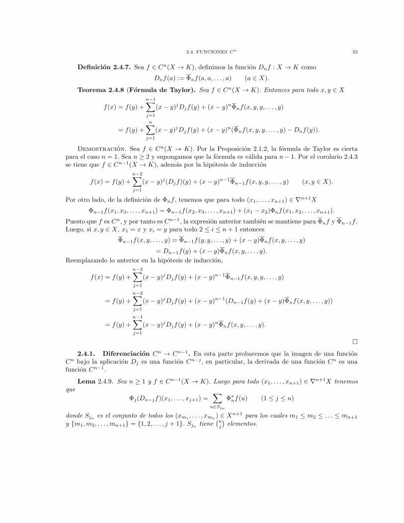
Definicion 2.4.7. Sea f ∈ Cn(X → K), definimos la funcion Dnf : X → K como
Dnf(a) := Φnf(a, a, . . . , a) (a ∈ X).
Teorema 2.4.8 (Formula de Taylor). Sea f ∈ Cn(X → K). Entonces para todo x, y ∈ X
f(x) = f(y) +
n−1∑
j=1
(x− y)jDjf(y) + (x− y)nΦnf(x, y, y, . . . , y)
= f(y) +
n∑
j=1
(x− y)jDjf(y) + (x− y)n(Φnf(x, y, y, . . . , y)−Dnf(y)).
Demostracion. Sea f ∈ Cn(X → K). Por la Proposicion 2.1.2, la formula de Taylor es ciertapara el caso n = 1. Sea n ≥ 2 y supongamos que la formula es valida para n− 1. Por el corolario 2.4.3se tiene que f ∈ Cn−1(X → K), ademas por la hipotesis de induccion
f(x) = f(y) +
n−2∑
j=1
(x− y)j(Djf)(y) + (x− y)n−1Φn−1f(x, y, y, . . . , y) (x, y ∈ X).
Por otro lado, de la definicion de Φnf , tenemos que para todo (x1, . . . , xn+1) ∈ ∇n+1X
Φn−1f(x1, x3, . . . , xn+1) = Φn−1f(x2, x3, . . . , xn+1) + (x1 − x2)Φnf(x1, x2, . . . , xn+1).
Puesto que f es Cn, y por tanto es Cn−1, la expresion anterior tambien se mantiene para Φnf y Φn−1f .Luego, si x, y ∈ X, x1 = x y xi = y para todo 2 ≤ i ≤ n+ 1 entonces
Φn−1f(x, y, . . . , y) = Φn−1f(y, y, . . . , y) + (x− y)Φnf(x, y, . . . , y)
= Dn−1f(y) + (x− y)Φnf(x, y, . . . , y).
Reemplazando lo anterior en la hipotesis de induccion,
f(x) = f(y) +
n−2∑
j=1
(x− y)jDjf(y) + (x− y)n−1Φn−1f(x, y, y, . . . , y)
= f(y) +
n−2∑
j=1
(x− y)jDjf(y) + (x− y)n−1(Dn−1f(y) + (x− y)Φnf(x, y, . . . , y))
= f(y) +
n−1∑
j=1
(x− y)jDjf(y) + (x− y)nΦnf(x, y, . . . , y).
�2.4.1. Diferenciacion Cn → Cn−1. En esta parte probaremos que la imagen de una funcion
Cn bajo la aplicacion Dj es una funcion Cn−j , en particular, la derivada de una funcion Cn es unafuncion Cn−1.
Lema 2.4.9. Sea n ≥ 1 y f ∈ Cn−1(X → K). Luego para todo (x1, . . . , xn+1) ∈ ∇n+1X tenemosque
Φj(Dn−jf)(x1, . . . , xj+1) =∑
u∈Sjn
Φ∗nf(u) (1 ≤ j ≤ n)
donde Sjn es el conjunto de todos los (xm1, . . . , xmn
) ∈ Xn+1 para los cuales m1 ≤ m2 ≤ . . . ≤ mn+1
y {m1,m2, . . . ,mn+1} = {1, 2, . . . , j + 1}. Sjn tiene(nj
)elementos.

2.4. FUNCIONES Cn 34
Demostracion. Un elemento de Sjn esta determinado por la cantidad de veces que aparece cada xi.Si ki es la cantidad de veces que aparece xi en un elemento x ∈ Sjn , entonces calcular |Sjn | equivale acalcular la cantidad de soluciones enteras de la ecuacion
k1 + k2 + . . .+ kj+1 = n+ 1
con ki ≥ 1, que es(n−j+j−1−1
n−j)
=(nn−j)
=(nj
). Para probar la formula, procederemos por induccion
sobre n ≥ 1. Supongamos que n = 1, entonces
Φ1(D0f)(x1, x2) =f(x1)− f(x2)
x1 − x2= Φ∗1f(x1, x2),
y la afirmacion es cierta en este caso.
Ahora supongamos que el lema es cierto para n−1 con n > 1. Debemos probar que la formula es ciertapara 2 ≤ j ≤ n. Sea (x1, . . . , xn+1) ∈ ∇n+1X. Por definicion de Φnf y por la hipotesis de induccion,tenemos que
Φj(Dn−jf)(x1, . . . , xj+1) =Φj−1(Dn−jf)(x1, x3, . . . , xj+1)− Φj−1(Dn−jf)(x2, . . . , xj+1)
x1 − x2
= (x1 − x2)−1
(∑
u∈AΦ∗n−1f(u)−
∑
u∈BΦ∗n−1f(u)
)
donde A y B son subconjuntos de {(xm1, . . . , xmn
) ∈ Xn : m1 ≤ . . . ≤ mn} determinado por{m1, . . . ,mn} = {1, 3, . . . , j + 1} y {m1, . . . ,mn} = {2, 3, . . . , j + 1} respectivamente. Si intercam-biamos 1 y 2 en A y B respectivamente, obtenemos una correspondencia u↔ u′ entre A y B.
Sea u = (u1, . . . , un) ∈ A. Luego existe k ≥ 1 tal que u1 = u2 = . . . = uk = x1 y uk+1 = x3, entonces
u = (x1, . . . , x1, uk+1, . . . , un)
y su correspondiente imagen u′ en B es
u′ = (x2, . . . , x2, uk+1, . . . , un).
Puesto que f ∈ Cn−1(X → K), por continuidad podemos extender el Lema 2.4.2 a Φn−1f y obtenemosque
Φ∗n−1f(u)− Φ∗n−1f(u′) = (x1 − x2)∑
t∈Au
Φ∗nf(t)
donde Au es el conjunto de todos los (xm1 , xm2 , . . . , xmn+1) ∈ Xn+1 tales que
m1 ≤ m2 ≤ . . . ≤ mk+1
{m1,m2, . . . ,mk+1} = {1, 2}(xmk+2
, . . . , xmn+1) = (uk+1, . . . , un)
{mk+2,mk+3, . . . ,mn+1} = {3, . . . , n+ 1}.Tenemos que Au ⊂ Sjn . Por otra parte, si v = (v1 . . . , vn+1) ∈ Sjn existe k1 ≥ 1 tal que vk1 = x2 yvk1+1 = x3, observamos que v ∈ Au con
u = (x1, . . . , x1, vk1+1, . . . , vn+1).
2.4. FUNCIONES Cn 35
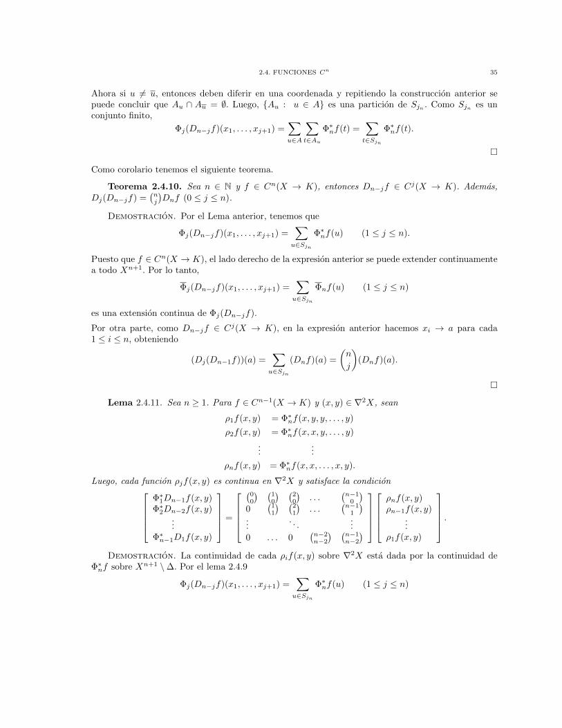
Ahora si u 6= u, entonces deben diferir en una coordenada y repitiendo la construccion anterior sepuede concluir que Au ∩ Au = ∅. Luego, {Au : u ∈ A} es una particion de Sjn . Como Sjn es unconjunto finito,
Φj(Dn−jf)(x1, . . . , xj+1) =∑
u∈A
∑
t∈Au
Φ∗nf(t) =∑
t∈Sjn
Φ∗nf(t).
�
Como corolario tenemos el siguiente teorema.
Teorema 2.4.10. Sea n ∈ N y f ∈ Cn(X → K), entonces Dn−jf ∈ Cj(X → K). Ademas,Dj(Dn−jf) =
(nj
)Dnf (0 ≤ j ≤ n).
Demostracion. Por el Lema anterior, tenemos que
Φj(Dn−jf)(x1, . . . , xj+1) =∑
u∈Sjn
Φ∗nf(u) (1 ≤ j ≤ n).
Puesto que f ∈ Cn(X → K), el lado derecho de la expresion anterior se puede extender continuamentea todo Xn+1. Por lo tanto,
Φj(Dn−jf)(x1, . . . , xj+1) =∑
u∈Sjn
Φnf(u) (1 ≤ j ≤ n)
es una extension continua de Φj(Dn−jf).
Por otra parte, como Dn−jf ∈ Cj(X → K), en la expresion anterior hacemos xi → a para cada1 ≤ i ≤ n, obteniendo
(Dj(Dn−1f))(a) =∑
u∈Sjn
(Dnf)(a) =
(n
j
)(Dnf)(a).
�
Lema 2.4.11. Sea n ≥ 1. Para f ∈ Cn−1(X → K) y (x, y) ∈ ∇2X, sean
ρ1f(x, y) = Φ∗nf(x, y, y, . . . , y)
ρ2f(x, y) = Φ∗nf(x, x, y, . . . , y)
......
ρnf(x, y) = Φ∗nf(x, x, . . . , x, y).
Luego, cada funcion ρjf(x, y) es continua en ∇2X y satisface la condicion
Φ∗1Dn−1f(x, y)Φ∗2Dn−2f(x, y)
...Φ∗n−1D1f(x, y)
=
(00
) (10
) (20
). . .
(n−1
0
)
0(
11
) (21
). . .
(n−1
1
)...
. . ....
0 . . . 0(n−2n−2
) (n−1n−2
)
ρnf(x, y)ρn−1f(x, y)
...ρ1f(x, y)
.
Demostracion. La continuidad de cada ρif(x, y) sobre ∇2X esta dada por la continuidad deΦ∗nf sobre Xn+1 \∆. Por el lema 2.4.9
Φj(Dn−jf)(x1, . . . , xj+1) =∑
u∈Sjn
Φ∗nf(u) (1 ≤ j ≤ n)

2.4. FUNCIONES Cn 36
donde Sjn es el conjunto de todos los (xm1 , . . . , xmn) ∈ Xn+1 para los cuales m1 ≤ m2 ≤ . . . ≤ mn+1 y{m1,m2, . . . ,mn+1} = {1, 2, . . . , j+1}. Puesto que Φ∗nf esta definida sobre Xn \∆, en el lado izquierode la expresion anterior hacemos x1 → x y xi → y si 2 ≤ i ≤ n. Luego,
lımx1→x, xi→y
Φj(Dn−jf)(x1, . . . , xj+1) = Φ∗j (Dn−jf)(x, y, . . . , y).
En el lado derecho, por argumentos combinatorios, observamos que existen(n−sj−1
)elementos de la forma
(u1, u2, . . . , un) tales que
u1 = u2 = . . . = us = x1, us+1 = x2.
Como las variables deben aparecer al menos una vez, s ∈ {1, . . . , n + 1 − j}. Si x1 → x y xi → y si2 ≤ i ≤ n en cada uno de estos elementos mencionados, observamos que
lımx1→x,xi→y
Φ∗nf(u) = ρsf(x, y).
Por lo tanto,
Φ∗j (Dn−jf)(x, y, . . . , y) =
n+1−j∑
s=1
(n− sj − 1
)ρsf(x, y) =
n−1∑
i=j−1
(i
j − 1
)ρn−if(x, y).
�
2.4.2. Antiderivacion Cn−1 → Cn.
Definicion 2.4.12. Sea n ∈ N \ {0}, f ∈ Cn−1(X → K). Consideramos xm como en la definicion2.2.1, es decir, xm = σm(x) donde (σm)m∈N es una aproximacion de la identidad. Escribimos
Pnf(x) :=∑
m∈N
n−1∑
j=0
f (j)(xm)
(j + 1)!(xm+1 − xm)j+1 (x ∈ X).
Probaremos que si f ∈ Cn−1(X → K) entonces la funcion Pnf es una antiderivada Cn de f . Para ello,estableceremos algunos resultados previos.
Teorema 2.4.13 (Formula de Taylor para Pnf). Sea n ∈ \{0}, f ∈ Cn−1(X → K). Luego
Pnf(x)− Pnf(y) =
n∑
j=1
(x− y)j
j!f (j−1)(y) + (x− y)nRn(x, y) (x, y ∈ X)
donde Rn(x, y) es una funcion continua que se anula en la diagonal ∆.
Demostracion. Definimos Rn : X ×X → K como
Rn(x, y) := (x− y)−n
Pnf(x)− Pnf(y)−
n∑
j=1
(x− y)j
j!f (j−1)(y)
.
Probaremos que efectivamente R(x, y) es una funcion continua sobre X ×X y que lımx,y→a
R(x, y) = 0
para cada a ∈ X. Recordemos que
Pnf(x) :=∑
m∈N
n−1∑
j=0
f (j)(xm)
(j + 1)!(xm+1 − xm)j+1 (x ∈ X).

2.4. FUNCIONES Cn 37
Por el Lema 2.4.9, f (j) ∈ Cn−j−1(X → K). Aplicando la formula de Taylor a f (j), para cada j ∈ Nexisten funciones continuas Λj : X ×X → K que se anulan en la diagonal tal que
f (j)(xm) =
n−j−1∑
s=0
(xm − y)s
s!f (s+j)(y) + (xm − y)n−j−1Λj(xm, y).
Reemplazando esta ultima expresion en la formula para Pnf(x), tenemos que
Pnf(x) =∑
m∈N
n−1∑
j=0
1
(j + 1)!
(n−j−1∑
s=0
(xm − y)s
s!f (s+j)(y) + (xm − y)n−j−1Λj(xm, y)
)(xm+1 − xm)j+1
=
n−1∑
k=0
((x− y)k− (x0− y)k)1
(k + 1)!f (k)(y) +
∑
m∈N
n−1∑
j=0
1
(j + 1)!(xm− y)n−j−1(xm+1−xm)j+1Λj(xm, y).
De la misma forma se tiene que
Pnf(y) =n−1∑
k=0
((y−y)k−(y0−y)k)1
(k + 1)!f (k)(y)+
∑
m∈N
n−1∑
j=0
1
(j + 1)!(ym−y)n−j−1(ym+1−ym)j+1Λj(ym, y)
Recordemos que x0 = y0, entonces
Pnf(x)−Pnf(y) =∑
m∈N
n−1∑
j=0
1
(j + 1)!
((xm − y)n−j−1(xm+1 − xm)j+1Λj(xm, y)
)−
n∑
j=1
(x− y)j
j!f j−1(y)
−∑
m∈N
n−1∑
j=0
1
(j + 1)!(ym − y)n−j−1(ym+1 − ym)j+1Λj(ym, y) +
n−1∑
k=0
(x− y)k1
(k + 1)!f (k)(y)
=∑
m∈N
n−1∑
j=0
1
(j + 1)!
((xm − y)n−j−1(xm+1 − xm)j+1Λj(xm, y)− (ym − y)n−j−1(ym+1 − ym)j+1Λj(ym, y)
).
Luego,v(Pnf(x)− Pn(y))
≤ maxm∈N, 1≤j≤n−1
{v((xm−y)n−j−1(xm+1−xm)j+1Λj(xm, y)), v((ym−y)n−j−1(ym+1−ym)j+1Λj(ym, y))}.
Sea ε ∈ G. Como Λj(u, v) es continua en X ×X, existe s ∈ N tal que si max{v(x− a), v(y− a)} < g−1s
implica v(Λj(x, y)) < ε. Por otra parte, existe t ≥ s tal que xi = yi si 0 ≤ i ≤ t y xt+1 6= yt+1.
Observamos que g−1t+1 ≤ v(x− y) < g−1
t . Luego, si m ≥ tv(xm − y) = v(xm − x+ x− y) ≤ max{v(xm − x), v(x− y)} ≤ max{g−1
m , v(x− y)} = ε(v(x− y))n,
yv(xm+1 − xm) ≤ {v(xm+1 − x), v(xm − x)} ≤ g−1
m ≤ v(x− y).
Por lo tanto,
v((xm − y)n−j−1(xm+1 − xm)j+1Λj(xm, y)) ≤ (v(x− y))nv(Λj(xm, y)) ≤ (v(x− y))nε.
Si 0 ≤ t < m, observamos que v((xt−y)n−j−1(xt+1−xt)j+1Λj(xt, y)) = 0. De similar forma se pruebaque
v((ym − y)n−j−1(ym+1 − ym)j+1Λj(ym, y)) ≤ ε (∀m ∈ N).
Luego, si max{v(x− a), v(y − a)} < g−1s entonces v((x− y)nRn(x, y)) ≤ (v(x− y))nε, y eso concluye
la demostracion. �

2.4. FUNCIONES Cn 38
Lema 2.4.14. Sea n ∈ N \ {0}, f ∈ Cn−1(X → K) tal que f ′ ∈ Cn−1(X → K). Supongamos que
f(x) = f(y) +
n∑
j=1
(x− y)jf (j)(y)
j!+ (x− y)nRn(x, y) (x, y ∈ X),
donde Rn es una funcion continua y que se anula en la diagonal. Luego para cada a ∈ X y todo j con1 ≤ j ≤ n
lımx,y→a
ρjf(x, y) =f (n)(a)
n!,
donde cada ρj estan definidos en el lema 2.4.11.
Demostracion. Sean x, y ∈ X. Por la formula de Taylor tenemos que
f(x) = f(y) +
n−1∑
j=1
(x− y)jf (j)(y)
j!+ (x− y)n−1(Φnf(x, y, . . . , y)−Dn−1f(y)).
Igualando con la expresion de la hipotesis, obtenemos
f (n)(y)
n!+Rn(x, y) = (x− y)n−1(Φn−1f(x, y, . . . , y)−Dn−1f(y))
= Φ∗nf(x, y, . . . , y) = ρ1f(x, y).
Puesto que Rn es continua y se anula en la diagonal ∆,
lımx,y→a
ρ1f(x, y) =f (n)(a)
n!.
Consideremos la expresion obtenida en la demostracion del Teorema 2.4.11,
Φ∗j (Dn−jf)(x, y, . . . , y) =
n−1∑
i=j−1
(i
j − 1
)ρn−if(x, y).
Si j = n− 1,
Φ∗n−1(D1f)(x, y, . . . , y) =
n−1∑
i=n−2
(i
n− 2
)ρn−if(x, y)
=
(n− 2
n− 2
)ρ2f(x, y) +
(n− 1
n− 2
)ρ1f(x, y)
= ρ2f(x, y) + nρ1f(x, y).
Despejando ρ2f(x, y), obtenemos
ρ2f(x, y) = Φ∗n−1(D1f)(x, y, . . . , y)− nρ1f(x, y).
Si x, y → a, por el Teorema 2.4.10
lımx,y→a
ρ2f(x, y) =
(n
n− 1
)(Dnf)(a)− (n− 1)
f (n)(a)
n!
= nf (n)(a)
n!− (n− 1)
f (n)(a)
n!=f (n)(a)
n!.

2.4. FUNCIONES Cn 39
De similar forma se prueba que si j = n− 2, entonces lımx,y→a
ρ3f(x, y) =f (n)(a)
n!. Repitiendo recursiva-
mente el proceso para j = n− 2, n− 3, . . . , 1 se prueba que
lımx,y→a
ρn−jf(x, y) =f (n)(a)
n!.
�Lema 2.4.15. Sea n ≥ 1 y f ∈ Cn−1(X → K). Sean B y S bolas en K. Supongamos que para
cada j ∈ {1, 2, . . . , n}ρjf(x, y) ∈ S (x, y ∈ B ∩X,x 6= y).
Luego, Φ∗nf(x1, . . . , xn+1) ∈ S para todo (x1, x2, . . . , xn+1) ∈ Xn+1 \ ∆ tal que xi ∈ B para cadai ∈ {1, 2 . . . , n}
Demostracion. Sea Λ := {(x1, . . . , xn+1) ∈ Xn+1\∆ : xi ∈ B para cada i}. Para j ∈ {2, . . . , n+1}, sea
Λj := {(x1, . . . , xn+1) ∈ Λ : {x1, x2, . . . , xn+1} tiene exactamente j elementos distintos entre si}.Luego Λ =
⋃n+1j=2 Λj . Puesto que cada ρj(x, y) ∈ S, observamos que Φ∗nf(Λ2) ⊂ S.
Supongamos que el Lema es cierto para j − 1 con 3 ≤ j ≤ n + 1. Probaremos que cada elemento deΦ∗nf(Λj) es una combinacion convexa de elementos de Φ∗nf(Λj−1). Sea u ∈ Λj . Por la simetrıa de Φ∗nf ,podemos suponer sin perder generalidad que u es de la forma
u = (x1, . . . , x1, x2, . . . , x2, . . . , x3, . . .)
tal que x1, x2, x3 son distintos entre sı, y que v(x1 − x2) ≥ max{v(x1 − x3), v(x2 − x3)}. Supongamosque x1 se repite k veces y que x2 se repite l veces, entonces por simplicidad denotamos u de la siguienteforma:
u = (xk1 , xl2, x3, . . .).
Aplicando el Lema 2.4.2 parte 1 a Φ∗nf , observamos que
Φ∗nf(xk1 , xl2, x3, . . .) =
x1 − x3
x1 − x2Φ∗nf(xk1 , x
l−12 , x3, . . .) +
x2 − x3
x1 − x2Φ∗nf(xk−1
1 , xl2, x3, . . .),
y esta es una combinacion convexa. Si l − 1 ≥ 1, podemos continuar escribiendo Φ∗nf(xk1 , xl−12 , x3, . . .)
como combinacion lineal convexa de Φ∗nf(xk1 , xl−22 , x3, . . .) y Φ∗nf(xk1 , x
l−12 , x3, . . .). De la misma forma
podemos continuar si k − 1 ≥ 1. Por lo tanto, podemos escribir Φ∗nf(u) como combinacion convexade elementos de la forma Φ∗n(v) donde v = (x3, . . .), lo que implica que v ∈ Λj−1. Por la hipotesis deinduccion, tenemos que Φ∗n(v) ∈ S y por lo anterior podemos concluir que Φ∗n(u) ∈ S. �
Lema 2.4.16. Sea n ∈ N \ {0} y sea f diferenciable tal que f ′ ∈ Cn−1(X → K). Supongamos que
f(x) = f(y) +
n∑
j=1
(x− y)jf (j)(y)
j!+ (x− y)nRn(x, y) (x, y ∈ X),
donde Rn(x, y) es una funcion continua que se anula sobre la diagonal ∆. Luego, f ∈ Cn(X → K).
Demostracion. Procedemos por induccion sobre n ≥ 1. El caso n = 1 viene de la definicion deΦ1f . Supongamos que es cierto para n− 1 con n > 1, entonces tenemos que f ∈ Cn−1(X → K). Porel Lema 2.4.14 tenemos que
lımx,y→a
ρj(x, y) =f (n)(a)
n!
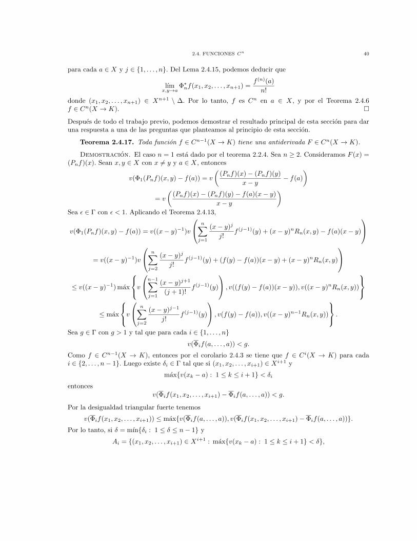
2.4. FUNCIONES Cn 40
para cada a ∈ X y j ∈ {1, . . . , n}. Del Lema 2.4.15, podemos deducir que
lımx,y→a
Φ∗nf(x1, x2, . . . , xn+1) =f (n)(a)
n!
donde (x1, x2, . . . , xn+1) ∈ Xn+1 \ ∆. Por lo tanto, f es Cn en a ∈ X, y por el Teorema 2.4.6f ∈ Cn(X → K). �
Despues de todo el trabajo previo, podemos demostrar el resultado principal de esta seccion para daruna respuesta a una de las preguntas que planteamos al principio de esta seccion.
Teorema 2.4.17. Toda funcion f ∈ Cn−1(X → K) tiene una antiderivada F ∈ Cn(X → K).
Demostracion. El caso n = 1 esta dado por el teorema 2.2.4. Sea n ≥ 2. Consideramos F (x) =(Pnf)(x). Sean x, y ∈ X con x 6= y y a ∈ X, entonces
v(Φ1(Pnf)(x, y)− f(a)) = v
((Pnf)(x)− (Pnf)(y)
x− y − f(a)
)
= v
((Pnf)(x)− (Pnf)(y)− f(a)(x− y)
x− y
)
Sea ε ∈ Γ con ε < 1. Aplicando el Teorema 2.4.13,
v(Φ1(Pnf)(x, y)− f(a)) = v((x− y)−1)v
n∑
j=1
(x− y)j
j!f (j−1)(y) + (x− y)nRn(x, y)− f(a)(x− y)
= v((x− y)−1)v
n∑
j=2
(x− y)j
j!f (j−1)(y) + (f(y)− f(a))(x− y) + (x− y)nRn(x, y)
≤ v((x− y)−1) max
v
n−1∑
j=1
(x− y)j+1
(j + 1)!f (j−1)(y)
, v((f(y)− f(a))(x− y)), v((x− y)nRn(x, y))
≤ max
v
n∑
j=2
(x− y)j−1
j!f (j−1)(y)
, v(f(y)− f(a)), v((x− y)n−1Rn(x, y))
.
Sea g ∈ Γ con g > 1 y tal que para cada i ∈ {1, . . . , n}v(Φif(a, . . . , a)) < g.
Como f ∈ Cn−1(X → K), entonces por el corolario 2.4.3 se tiene que f ∈ Ci(X → K) para cadai ∈ {2, . . . , n− 1}. Luego existe δi ∈ Γ tal que si (x1, x2, . . . , xi+1) ∈ Xi+1 y
max{v(xk − a) : 1 ≤ k ≤ i+ 1} < δi
entoncesv(Φif(x1, x2, . . . , xi+1)− Φif(a, . . . , a)) < g.
Por la desigualdad triangular fuerte tenemos
v(Φif(x1, x2, . . . , xi+1)) ≤ max{v(Φif(a, . . . , a)), v(Φif(x1, x2, . . . , xi+1)− Φif(a, . . . , a))}.Por lo tanto, si δ = mın{δi : 1 ≤ δ ≤ n− 1} y
Ai = {(x1, x2, . . . , xi+1) ∈ Xi+1 : max{v(xk − a) : 1 ≤ k ≤ i+ 1} < δ},

2.5. EL TEOREMA DE LA FUNCION INVERSA PARA FUNCIONES Cn. 41
entonces tenemos que para todo 1 ≤ i ≤ n− 1
sup{v(Φif(x1, x2, . . . , xi+1)) : (x1, x2, . . . , xi+1) ∈ Ai} ≤ g.Sea y ∈ X tal que v(y − a) < δ. Hacemos xk → y, y obtenemos que para todo j ∈ {2, . . . , n}
v(f (j−1)(y)) = v((j − 1)!Dj−1f(y)) ≤ g.
Dada la continuidad de f y Rn(x, y) en X, existen r1, r2 ∈ Γ tales que
(v(y − a) < r2)⇒ (v(f(y)− f(a)) < ε),
(max{v(x− a), v(y − a)} < r1)⇒ (v(R(x, y)) < ε).
Finalmente, si consideramos r = mın{r1, r2, δ, ε, 1} tenemos que v((x− y)n−1) ≤ 1 y
v(Φ1(Pnf)(x, y)− f(a)) ≤ max{v((x− y)j−1f (j−1)(y)), v(f(y)− f(a)), v((x− y)n−1Rn(x, y))
}
≤ max{gε, ε, gε}.Por lo tanto (Pnf)′ = f .
Para la otra parte de la afirmacion, por el teorema 2.4.13
Pnf(x)− Pnf(y) =
n∑
j=1
(x− y)j
j!f (j−1)(y) + (x− y)nRn(x, y)
=
n∑
j=1
(x− y)j
j!((Pnf)′)(j−1)(y) + (x− y)nRn(x, y)
=
n∑
j=1
(x− y)j
j!(Pnf)(j)(y) + (x− y)nRn(x, y).
Por el lema 2.4.16 se tiene que Pnf , que es una antiderivada de f , pertenece a Cn(X → K). �
2.5. El teorema de la funcion inversa para funciones Cn.
Lema 2.5.1. Sea f : X → K una funcion inyectiva y sea g : f(X) → X su inversa. Sea n ∈ Ncon n ≥ 2, y sea Sn el conjunto formado por las siguientes funciones definidas sobre ∇n+1f(X)
(x1, x2, . . . , xn+1) 7→ Φ1g(xi1 , xi2) (i1 < i2)
(x1, x2, . . . , xn+1) 7→ Φ2g(xi1 , xi2 , xi3) (i1 < i2 < i3)
...
(x1, x2, . . . , xn+1) 7→ Φn−1g(xi1 , . . . , xin) (i1 < i2 < . . . < in)
y
(x1, x2, . . . , xn+1) 7→ Φ1f(g(xi1), g(xi2)) (i1 < i2)
(x1, x2, . . . , xn+1) 7→ Φ2f(g(xi1), g(xi2), g(xi3)) (i1 < i2 < i3)
...
(x1, x2, . . . , xn+1) 7→ Φn−1f(g(xi1), . . . , g(xin)) (i1 < i2 < . . . < in)
(x1, x2, . . . , xn+1) 7→ Φn−1f(g(x1), g(x2), . . . , g(xn), g(xn+1))
Sea Rn el anillo generado por Sn. Luego Φng ∈ Rn.
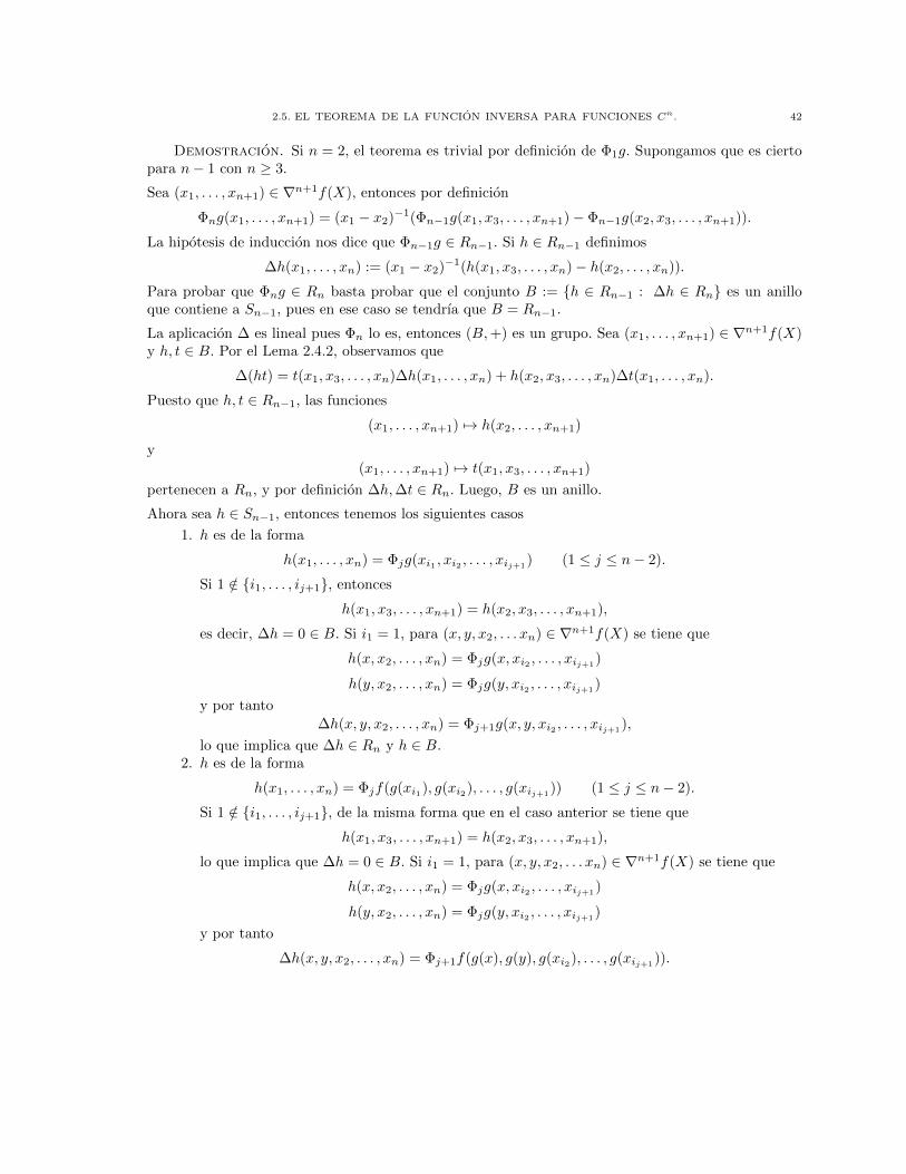
2.5. EL TEOREMA DE LA FUNCION INVERSA PARA FUNCIONES Cn. 42
Demostracion. Si n = 2, el teorema es trivial por definicion de Φ1g. Supongamos que es ciertopara n− 1 con n ≥ 3.
Sea (x1, . . . , xn+1) ∈ ∇n+1f(X), entonces por definicion
Φng(x1, . . . , xn+1) = (x1 − x2)−1(Φn−1g(x1, x3, . . . , xn+1)− Φn−1g(x2, x3, . . . , xn+1)).
La hipotesis de induccion nos dice que Φn−1g ∈ Rn−1. Si h ∈ Rn−1 definimos
∆h(x1, . . . , xn) := (x1 − x2)−1(h(x1, x3, . . . , xn)− h(x2, . . . , xn)).
Para probar que Φng ∈ Rn basta probar que el conjunto B := {h ∈ Rn−1 : ∆h ∈ Rn} es un anilloque contiene a Sn−1, pues en ese caso se tendrıa que B = Rn−1.
La aplicacion ∆ es lineal pues Φn lo es, entonces (B,+) es un grupo. Sea (x1, . . . , xn+1) ∈ ∇n+1f(X)y h, t ∈ B. Por el Lema 2.4.2, observamos que
∆(ht) = t(x1, x3, . . . , xn)∆h(x1, . . . , xn) + h(x2, x3, . . . , xn)∆t(x1, . . . , xn).
Puesto que h, t ∈ Rn−1, las funciones
(x1, . . . , xn+1) 7→ h(x2, . . . , xn+1)
y(x1, . . . , xn+1) 7→ t(x1, x3, . . . , xn+1)
pertenecen a Rn, y por definicion ∆h,∆t ∈ Rn. Luego, B es un anillo.
Ahora sea h ∈ Sn−1, entonces tenemos los siguientes casos
1. h es de la forma
h(x1, . . . , xn) = Φjg(xi1 , xi2 , . . . , xij+1) (1 ≤ j ≤ n− 2).
Si 1 /∈ {i1, . . . , ij+1}, entonces
h(x1, x3, . . . , xn+1) = h(x2, x3, . . . , xn+1),
es decir, ∆h = 0 ∈ B. Si i1 = 1, para (x, y, x2, . . . xn) ∈ ∇n+1f(X) se tiene que
h(x, x2, . . . , xn) = Φjg(x, xi2 , . . . , xij+1)
h(y, x2, . . . , xn) = Φjg(y, xi2 , . . . , xij+1)
y por tanto∆h(x, y, x2, . . . , xn) = Φj+1g(x, y, xi2 , . . . , xij+1
),
lo que implica que ∆h ∈ Rn y h ∈ B.2. h es de la forma
h(x1, . . . , xn) = Φjf(g(xi1), g(xi2), . . . , g(xij+1)) (1 ≤ j ≤ n− 2).
Si 1 /∈ {i1, . . . , ij+1}, de la misma forma que en el caso anterior se tiene que
h(x1, x3, . . . , xn+1) = h(x2, x3, . . . , xn+1),
lo que implica que ∆h = 0 ∈ B. Si i1 = 1, para (x, y, x2, . . . xn) ∈ ∇n+1f(X) se tiene que
h(x, x2, . . . , xn) = Φjg(x, xi2 , . . . , xij+1)
h(y, x2, . . . , xn) = Φjg(y, xi2 , . . . , xij+1)
y por tanto
∆h(x, y, x2, . . . , xn) = Φj+1f(g(x), g(y), g(xi2), . . . , g(xij+1)).

2.5. EL TEOREMA DE LA FUNCION INVERSA PARA FUNCIONES Cn. 43
Luego ∆h es un producto de dos funciones en Sn. Por lo tanto ∆h ∈ Rn y h ∈ B.
�Tenemos el teorema central de esta seccion,
Teorema 2.5.2 (Teorema de la funcion inversa para funciones Cn). Sea f ∈ Cn(X → K)y sea a ∈ X tal que f ′(a) 6= 0. Entonces existe una vecindad U de a tal que f : U ∩X → f(U ∩X) esinyectiva y su inversa local g : f(U ∩X)→ U ∩X es una funcion Cn.
Demostracion. Procedemos por induccion sobre n. El caso n = 1 esta dado por el Teorema2.1.3. Supongamos que el Teorema es cierto para el caso n− 1 con n > 1.
Sea f ∈ Cn(X → K) y a ∈ X tal que f ′(a) 6= 0, entonces por la hipotesis de induccion existe unavecindad U de a tal que f es inyectiva en U ∩ X y su inversa local g : f(U ∩ X) → U ∩ X es unafuncion Cn−1.
Para probar que g ∈ Cn(X → K), aplicamos el Lema anterior a f y g, y tenemos que Φng ∈ Rn.Como f, g ∈ Cn−1(X → K), las funciones que pertenecen a Rn pueden extenderse continuamente a(f(U ∩X))n+1. Eso termina la demostracion. �

Capıtulo 3
Conjuntos no medibles en el cuerpo de Levi-Civita
En [6], K. Shamseddine y M. Berz establecieron una Teorıa de la Medida en el cuerpo de Levi-Civita,R, que les permite definir funciones medibles en subconjuntos medibles y con ello la integral de talesfunciones. Todas sus definiciones y teoremas se dan en el marco del orden de este cuerpo. Pero Radmite tambien una valuacion no arquimediana v, que es compatible con el orden en el sentido que|a| ≤ |b| ⇒ v(a) ≤ v(b) . Por tanto la pregunta que surge naturalmente es por la medida de la bolaunitaria B0(1) = {x ∈ R : v(x) ≤ 1}.En el artıculo que se adjunta como Anexo 2 se establece que B0(1) no es medible, y como corolarioobtenemos que todo intervalo (a, b) ⊂ R contiene una infinitud de subconjuntos convexos que no sonmedibles. Presentamos aquı un resumen, primeramente se describira el cuerpo de Levi-Civita y luegose citan los resultados principales.
3.1. Preliminares: El cuerpo de Levi-Civita.
Definicion 3.1.1. Un subconjunto S ⊂ Q se llama finito-izquierdo si para cada q ∈ Q el conjunto{s ∈ S : s < q} es finito.Consideramos el conjunto de las funciones F = {x : Q → R} y sea supp(x) = {s ∈ Q : x(s) 6= 0} elsoporte de x. Entonces definimos el cuerpo de Levi-Civita por
R := {x ∈ F : supp(x) es finito izquierdo}.
Notacion: Sea x ∈ R, la imagen de un elemento q ∈ Q bajo x se denota por x[q] y sera λ(x) :=mın supp(x) si x 6= 0, λ(x) :=∞ si x = 0.
Definimos la suma y multiplicacion en R por
(x+ y)[q] = x[q] + y[q],
(x · y)[q] =∑
qx+qy=q
x[qx]y[qy].
La multiplicacion en R esta bien definida, pues para cada q ∈ Q existe una cantidad finita de sumandos
en∑
qx+qy=q
x[qx]y[qy]. Se prueba directamente que (R,+, ·) es efectivamente un cuerpo. Cada numero
real r se puede identificar en R con la funcion r : Q→ R definida por
r[q] =
{0 if q 6= 0r if q = 0
,
mas aun, esta asignacion es un isomorfismo de anillos . Por lo tanto R extiende al cuerpo R .
Definimos ahora un orden en R: Sean x 6= y en R, diremos que x ≤ y si (x− y)[λ(x− y)] < 0. Comoes usual, x ≥ y si y ≤ x. La relacion binaria ≤ es un orden lineal y (R,≤) es un cuerpo ordenado. El
44
3.2. CONJUNTOS NO MEDIBLES EN R 45
orden ≤ induce un valor absoluto | | en el sentido usual, es decir, |x| = max{x,−x} para todo x ∈ R.Notamos ademas que este orden es no-arquimediano, ya que N es acotado por cualquier funcion x talque λ(x) > 0 y x[λ(x)] > 0 en R.
Por otra parte, definimos la funcion v : R → R+ por
v(x) =
{e−λ(x) si x 6= 00 si x = 0
.
Se verifica directamente que v es una valuacion no arquimediana en R que, como en [5] 1.4.1, defineuna ultrametrica. La valuacion v es compatible con el orden definido anteriormente en el siguientesentido, para todo a, b ∈ R con |a| ≤ |b| entonces v(a) ≤ v(b). Equivalentemente, si v(a) > v(b) implicaque |a| > |b|.
Definicion 3.1.2. El elemento d ∈ R es la funcion definida por d[1] = 1 y d[q] = 0 si q 6= 1.
Observamos que para n ≥ 1
dn[q] =
{0 si q 6= n1 si q = n
.
El orden y la valuacion v inducen una topologıa en R respectivamente. Tenemos que estas topologıasson iguales, esta topologıa en comun la denotamos por τ . (R, τ) es un espacio ultrametrico, completopues las sucesiones de Cauchy en R convergen. Observamos que la sucesion (dn)n∈N es estrictamentedecreciente y que lım
n→∞dn = 0, por lo tanto es una sucesion coinicial en R+ \ {0}.
3.2. Conjuntos no medibles en REn lo que sigue, Ia,b es un intervalo en R con puntos finales a, b (a < b) de la forma (a, b), [a, b], (a, b] o[a, b). El largo de un intervalo I = Ia,b es l(I) := b− a. Las siguientes definiciones fueron introducidaspor K. Shamseddine y M. Berz, para mas detalles ver [6].
Definicion 3.2.1. Diremos que A ⊂ R es medible si para todo n ∈ N existen conjuntos {Ink :k ∈ N} y {Jnk : k ∈ N} de intervalos disjuntos dos a dos contenidos en R tales que
∞⋃
k=0
Jnk ⊂ A ⊂∞⋃
k=0
Ink ,
las series∑∞k=0 l(I
nk ) and
∑∞k=0 l(J
nk ) convergen en R, y∣∣∣∣∣∞∑
k=0
l(Ink )−∞∑
k=0
l(Jnk )
∣∣∣∣∣ < dn.
Observamos que en esta definicion si m > n el conjunto de intervalos {Imk : k ∈ N} (respectivamente{Jmk : k ∈ N}) no tiene necesariamente relacion con {Ink : k ∈ N} (respectivamente {Jnk : k ∈ N}).Para obtener el resultado deseado fue necesario demostrar el siguiente lema, (mencionado en [6]).
Lema 3.2.2 ([2], 2.4). Sea A un conjunto medible, entonces para todo n ∈ N existen colecciones{Ink : k ∈ N} y {Jnk : k ∈ N} de intervalos contenidos en R disjuntos dos a dos tales que
∞⋃
k=0
Jn−1k ⊂
∞⋃
k=0
Jnk ⊂ A ⊂∞⋃
k=0
Ink ⊂∞⋃
k=0
In−1k ,

3.2. CONJUNTOS NO MEDIBLES EN R 46
las series∑∞k=0 l(I
nk ) y
∑∞k=0 l(J
nk ) convergen en R, y
∞∑
k=0
l(Ink )−∞∑
k=0
l(Jnk ) < dn.
Mas aun los lımites
lımn→∞
∞∑
k=0
l(Ink ) y lımn→∞
∞∑
k=0
l(Jnk )
existen en R y son iguales.
Podemos ahora definir una medida µ.
Definicion 3.2.3. Sea A la clase de los conjuntos medibles enR. Definimos la funcion µ : A→ R+
por:
µ(A) := lımn→∞
∞∑
k=0
l(Ink ) = lımn→∞
∞∑
k=0
l(Jnk ),
Utilizando el lema 3.2.2, en [2] se prueba que µ es una funcion bien definida, en el sentido de que si Aes medible entonces µ(A) es independiente de la eleccion de las colecciones de intervalos {Ink : k ∈ N}y {Jnk : k ∈ N} que satisfacen las condiciones de la definicion 3.2.1.
Teorema 3.2.4 ([2]). µ satisface las siguientes propiedades:
µ(I) = l(I) para todo intervalo I = Ia,b.
Si {Ek}∞k=0 es una sucesion de intervalos de R disjuntos dos a dos tales que l(Ek) ∈ R+ y∞∑
k=0
l(Ek) converge en R, entonces
µ
( ∞⋃
k=0
Ek
)=
∞∑
k=0
l(Ek).
Si A es medible entonces A+ λ tambien lo es, y µ(A) = µ(A+ λ) para todo λ ∈ R.
Con respecto a la monotonıa de µ citamos a [6], pg. 377: Si B ⊂ A ⊂ R y si A, B ası como A \B sonmedibles, entonces µ(B) ≤ µ(A).
El resultado principal, de este capıtulo son los dos teoremas siguientes:
Teorema 3.2.5 ([2], 2.6). Para todo δ ∈ R se tiene que la bola
B0(δ) = {x ∈ R : v(x) ≤ δ}no es medible. En particular, la bola unitaria B0(1) no es medible.
Ahora consideramos un intervalo Ia,b en R. Dado que la valuacion v es compatible con el ordendefinido en R, para todo x0 ∈ Ia,b existe ε ∈ R tal que Bx0
(ε) ⊂ Ia,b. Si Bx0(ε) fuese medible entonces
B0(ε) = −x0 +Bx0(ε) tambien lo serıa, lo que contradice el teorema 3.2.5. Por tanto:
Teorema 3.2.6 ([2], 2.7). Todo intervalo Ia,b en R contiene un subconjunto convexo no vacıo Cque no es medible.

3.2. CONJUNTOS NO MEDIBLES EN R 47
Como R es ordenado y completo, cada intervalo contiene Ia,b con a < b contiene infinitos puntos x0
que son distintos de a y b, lo que establece el siguiente corolario:
Corolario 3.2.7 ([2], 2.8). Todo intervalo Ia,b contiene infinitos conjuntos convexos que no sonmedibles.

Bibliografıa
[1] H. M. Moreno, Toward an ultrametric calculus in a field K with an infinite rank valuation, in Advances in non-
Archimedean Analysis, Contemp. Math., vol. 551, Amer. Math. Soc., Providence, RI, 2011, pp. 221-230.[2] H. M. Moreno, Non-measurable sets in the Levi-Civita field, in Advance in Ultrametric Analysis, Contemp. Math.,
vol. 596, Amer. Math. Soc., Providence, RI, 2013, pp. 163-177.
[3] W.H. Schikhof, Ultrametric calculus: An introduction to p-adic analysis, Cambridge Studies in Advanced Mathe-matics 4. Cambridge University Press (1984).
[4] H. Keller, Ein nicht-klassischer Hilbertscher Raum, Math Z. 172 (1980), 41 − 49.
[5] H. Ochsenius and W. Schikhof, Banach spaces over fields with an infinite rank valuation, In p-Adic FunctionalAnalysis, Lecture Notes in pure and applied mathematics 207, edited by J. Kakol, N. De Grande-De Kimpe and C.
Perez-Garcia. Marcel Dekker (1999), 233-293.
[6] K. Shamseddine and M. Berz, Measure theory and integration in Levi-Civita field. Contemp. Math. 319, Amer.Math. Soc. (2003), 369 − 387.
[7] K. Shamseddine and M. Berz, Convergence on the Levi-Civita field and study of power series, Lecture Notes in
Pure and Applied Mathematics, Marcel Dekker (2000), 283-299.[8] M.P. Soler, Characterization of Hilbert spaces by orthomodular spaces. Communications in Algebra 23 (1995),
219 − 243.[9] P. Ribenboim, Theorie des valuations. Deuxieme edition multigraphiee. Seminaire de Mathematiques Superieures,
No. 9 (Ete, 1964), Les Presses de l’Universitde Montreal, Montreal, Que. 1968.
48

This is a free offprint provided to the author by the publisher. Copyright restrictions may apply.
Toward an ultrametric calculus in a field K with an infiniterank valuation.
Hector M. Moreno
Abstract. K is the scalar field of the first orthomodular (or Form Hilbert) space, described by H. Keller in 1980. It has a non-archimedean order,an infinite rank valuation as well as an explicitly defined ultrametric, all ofwhich induce the same topology. We will present results concerning analyticfunctions, and show some examples that sharply contrast with the case of rank
one valuations. Finally we prove a theorem concerning local invertibility forC1 functions.
1. Introduction
Ultrametric Calculus over valued fields of rank one is a well developed theory (see[1] ), and for the last years it has been studied in the case of the field of Levi Civita,where the valuation has rank 1. In the case of fields with valuations of infinite rank,R. Hobeika (Ph.D Thesis, University of Paris VI, 1976) studied power series anLaurent series on Krull valued fields F , and showed that the domain of convergenceof a power series is either K or reduced to a point. Therefore the classical definitionof an analytic function on an open subset only gives entire functions on K. Y.Perrin extended the notion of analytic functions on an open subset, following ideasof Krasner ([3]) and studied properties of these functions (algebraic operations,derivation, characterization of the set of their zeros, Weierstrass theorem, Mittag-Leffler theorem). (See [4], [5], [6] and [7]). However the fields she considers arealways algebraically closed.
We approach the study of ultrametric calculus from another direction. We willconsider here the field K, described in [2]. Its importance comes from the factthat it is the prototypical canonical example of a scalar field for orthomodular non-classical spaces of Hilbert type. According to the theorem of M.P. Soler (see [8]),these fields can never be algebraically closed. K has a non-archimedean order, whichextends the usual ordering of its subfield R. This order induces an ultrametrizabletopology, that is also generated by a valuation v of infinite rank. A crucial differencewith the Levi Civita field, that is also an ordered field, is the fact that there is nodistinguished element d > 0 such that
∀ε > 0 ∃k ∈ N (dk < ε),
2000 Mathematics Subject Classification. Primary 46S10; Secundary 46H35.Key words and phrases. ultrametric calculus, valued fields, analytic functions.Partially suported by Fondecyt Proyecto 1080194.
1
Contemporary MathematicsVolume 551, 2011
221

This is a free offprint provided to the author by the publisher. Copyright restrictions may apply.
2 HECTOR M. MORENO
but instead ”infinitely many degrees of infinity”. This has as a consequence thatK has properties that sharply contrast with these fields as well as with the clas-sical fields of reals or complex numbers. We recall for instance that the region ofconvergence of power series is either one point, or the whole K, and there existselements z ∈ K such that 0 < z < 1 but the sequence {zn} does not convergeto zero. In this paper we aim to give an introduction to Ultrametric Calculus inK. We describe in the Preliminaries the field K, its ordering and the valuation v.Then we show results for analytic functions that are clearly different from the caseof rank one, or that coincide with them but with completely different proofs. Wealso give counterexamples to some theorems for the real or complex case.
2. Preliminaries
2.1. The field K. Let us consider F0 = R with its usual ordering, and theset of variables {X1, X2, X3, . . .}. For any n ≥ 1 define Fn : = F0(X1, . . . , Xn) andlet
F∞ : =∞∪
n=0Fn
.
We order Fn by powers of Xn, a polynomial P (Xn) = a0 + a1Xn + ... + asXsn ∈
Fn−1[Xn] is positive in Fn if and only if as > 0 in Fn−1. For λ ∈ Fn, λ =p(Xn)
q(Xn)with p(Xn), q(Xn) ∈ Fn−1[Xn] and q(Xn) �= 0, we shall say that λ is a positiveelement in Fn if and only if p(Xn)q(Xn) > 0. Since the ordering of Fn extends theordering of Fn−1, F∞ is an ordered field. In fact given λ ∈ F∞ there exists n ∈ Zsuch that λ ∈ Fn, hence λ > 0 in F∞ if and only if the same is true in Fn. Noticethat this ordering is non-archimedean.
As usual |λ| will denote the absolute value of λ ∈ F∞, that is to say,
|λ| =
{λ, if λ ≥ 0
−λ, if that is not the case.
The order of F∞, induces a topology in the field, which has as a base of zeroneighborhoods the collection of sets Uε = {a ∈ K : |a| < ε} for all ε in F∞.
We consider now a non-archimedean valuation in F∞. Firstly we define the valuegroup.For every i = 1, 2, 3, 4, ... we pick a real number gi > 1 and we consider the mul-tiplicative cyclic subgroup Gi generated by gi, ordered by the usual ordering of R.We define Γ by
Γ :=
{γ ∈ (gn1
1 , gn22 , gn3
3 , ..., gnii , ...) ∈
∞∏
i=1
Gi : ni ∈ Z such that supp(γ) is finite
},
with supp(γ) := {i ∈ N : ni �= 0}. Γ is a linearly ordered group with thecomponentwise operation and the antilexicographical ordering. The identity is1 = (1, 1, 1, 1, 1, ...).
For every m ≥ 1 we put
Hm = G1 × G2 × ... × Gm × {1} × {1} × ...
and then {1} = H0 ⊂ H1 ⊂ H2 ⊂ ... are the convex subgroups of Γ. Therefore thisis a group of infinite rank.
222
This is a free offprint provided to the author by the publisher. Copyright restrictions may apply.
TOWARD AN ULTRAMETRIC CALCULUS IN A FIELD K WITH AN INFINITE RANK VALUATION.3
The valuation v : F∞ → Γ ∪ {0} is the unique valuation defined on F∞ such that
(1) v|R is the trivial valuation(2) v(Xn) = gn := (1, ..., 1, gn, 1, ...).
where 0 is a minimal element adjoined to Γ such that 0 · g = g · 0 = 0.
Let r ∈ Γ and a ∈ F∞. The open ball with center a and radius r is the set
Ba(r−) = {x ∈ K : v(x − a) < r}.
Now we define an ultrametric in F∞. Let φ : F+∞ → R be given by
φ(α) =
⎧⎪⎪⎪⎪⎪⎪⎪⎨⎪⎪⎪⎪⎪⎪⎪⎩
2n+1 if Xsn < α ≤ Xr
n+1 for all s ∈ Z and some r ∈ Z+.2 if s < α < Xr
1 for all s ∈ Z+ and some r ∈ Z+.1 if 1
s ≤ α ≤ r, with r, s ∈ Z+.12 if 1
Xr1
< α < s for all s ∈ Z+ and some r ∈ Z+.
2−(n+1) if 1Xr
n+1< α ≤ 1
Xsn
for all s ∈ Z and some r ∈ Z+.
0 if α = 0.
where n ∈ Z+ \ {0}. A direct computation shows that the map d : F∞ × F∞ → R+
defined byd(x, y) = φ(|x − y|)
is indeed an ultrametric for F∞.
It can be proven directly that each of the following collections of subsets of F∞
Bo = {Oa(t−) : a, t ∈ F∞}Bd = {Ca(s−) : a ∈ F∞, s ∈ R+}Bv = {Ba(r−) : a ∈ F∞, r ∈ Γ}
whereOa(t−) = {x ∈ F∞ : |x − a| < t}
Ca(s−) = {x ∈ F∞ : d(x − a) < s}Ba(r−) = {x ∈ F∞ : v(x − a) < r}.
is a subbasis for a topology in K. But since for every x ∈ F∞ the following inclusionshold.
Cx
(1
2n−1
−)⊂ Ox
(1
Xn
−)⊂ Cx
(1
2n
−)
Ox
(1
Xn
−)⊂ Bx((g−1
n )−) ⊂ Ox
(1
Xn−1
−)
for every n ≥ 1, these topologies are identical. This common topology will bedenoted by τ .
(F∞, τ ) is an ultrametrizable topological space, therefore we can consider K thecompletion of F∞ by Cauchy sequences (nets). The topology in K is generated bythe extension of d to K,
d(x, y) = limn→∞
d(xn, yn)
where x, y ∈ K and (xn)n, (yn)n are sequences in F∞ such that limn→∞ xn = x ylimn→∞ yn = y.
Let a, b ∈ K and (an)n, (bn)n sequences in F∞ such that limn→∞ an = a andlimn→∞ bn = b. It can be proved directly that K is a field with the operationsa + b = limn→∞(an + bn), ab = limn→∞(anbn) and a−1 = limn→∞ a−1
n .
TOWARD AN ULTRAMETRIC CALCULUS IN A FIELD K 223

This is a free offprint provided to the author by the publisher. Copyright restrictions may apply.
4 HECTOR M. MORENO
On the other hand, we extend the order of F∞ to K by defining the binary relation≤ in K as a ≤ b if and only if a = b, or, a �= b and there exist sequences in F∞such that limn→∞ an = a, limn→∞ bn = b and (an − bn) ≤ 0 for all n ≥ N for someN ∈ N.
Proposition 2.1. (K, ≤) is an ordered field.
The order in K induces an absolute value, which will also be denoted by | |.Let a ∈ K with a �= 0, there exists a sequence (an)n in F∞ that converges to a.Hence, for some N ∈ N we have that
v(an) = v(an − aN + aN ) = v(aN ) (n ≥ N).
Therefore we can extend the valuation v of F∞ to K as v(a) = v(aN ), and it canbe proved directly that (K, v) is a valued field with a valuation of infinite rank.
As in the case of F∞, each of the maps d, v and | | induce the same topology τ inK, and (K, τ ) is a topological field. We remark that K is not locally compact since
{x ∈ K : v(x) ≤ 1} =⋃
a∈R(a + {x ∈ K : v(x) < 1}) =
⋃
a∈R{x ∈ K : v(x − a) < 1}
is a countable covering by disjoint open sets and thus it cannot have a finite sub-covering. This implies that the unit ball in K is not compact.
In addition K is not separable since R is an uncountable discrete set in K.
3. The Main Result.
An ultrametric calculus for the field K is currently being developed. New resultshave been obtained that sharply contrast with the case of fields with a rank onevaluation.
3.1. Analytic functions.
Definition 3.1. Let a0, a1, ... be a sequence in K. The power series∑∞
j=0 ajzj
is the sequence of polynomial functions en the variable z given by sn(z) =∑n
j=0 ajzj .
The region of convergence of the power series∑∞
j=0 ajzj is the set
{z ∈ K : (sn(z))n converges in K}
Theorem 3.2. A power series
∞∑
j=0
ajzj with aj ∈ K converges, for z �= 0, if
and only if limn→∞ an = 0.
Proof. Assume that the sequence is convergent, then limn→∞ anzn = 0. Letz be an element in K, there exist a convex subgroup Hm �= {Id} of Γ such thatfor all n ∈ N, v(zn) ∈ Hm. Choose y ∈ K such that v(y) ∈ Hm+1 \ Hm andv(y) < v(zn) for all n ∈ N. It follows that
v(an)v(y) < v(an)v(zn) → 0
when n → ∞. Therefore limn→∞ an = 0.
On the other hand, let us suppose that limn→∞ an = 0. For any z ∈ K and m ∈ Nsuch that v(z) ∈ Hm, choose y ∈ K with v(y) ∈ Hm+1 \Hm, v(zn) < v(y) for everyn ∈ N. Then
v(an)v(zn) < v(an)v(y) → 0
224

This is a free offprint provided to the author by the publisher. Copyright restrictions may apply.
TOWARD AN ULTRAMETRIC CALCULUS IN A FIELD K WITH AN INFINITE RANK VALUATION.5
when n → ∞, and the power series∑∞
j=0 ajzj converges in K. �
A direct consequence of Theorem 3.2 is the fact that the usual series expansion forthe exponential, logarithm, and trigonometric functions are not convergent in K.
Theorem 3.3. Let∑∞
n=0 anzn be a convergent power series in K. Then forevery a ∈ K this series converges uniformly in Ba(r), for all r ∈ Γ. The function
z �→∞∑
n=0
anzn (z ∈ K)
is differentiable and its derivative is the function
z �→∞∑
n=1
nanzn−1 (z ∈ K).
Proof. Let ε > 0 . Choose y /∈ Ba(r) such that v(y) > v(z) for every z ∈Ba(r). Since the series
∑∞n=0 anzn converges, we observe that limn→∞ an = 0, this
implies that there exists n0 ∈ N such tha maxn≥n0v(an)v(y) < ε. Hence for any
z ∈ Ba(r)
v
( ∞∑
n=n0
anzn
)≤ max
n≥n0
v(an)v(zn) ≤ maxn≥n0
v(an)v(y) < ε.
We conclude that the power series∑∞
n=0 anzn converges uniformly in Ba(r).
Since standard classical arguments hold true in this case, for the proof of the secondstatement it is enough to observe the following. For all n ≥ 1, v(nanzn−1) =v(z−1)v(anzn), hence the power series
∑∞n=1 nanzn−1 converges for all z ∈ K. �
Definition 3.4. Let D ⊆ K be a non-empty open set. A function f : D → Kis analytic in D if there are elements u ∈ D, r ∈ Γ and a0, a1, . . . ∈ K such that forevery z ∈ D
f(z) =
∞∑
n=0
an(z − u)n.
Let us now study the following situation. In the real or complex case, as well asin rank one valued fields, if f is a analytic in an open ball U and f(z) �= 0 for anyz ∈ U then 1
f is analytic in U .
The following example shows that this statement is false in K.
Example 3.5. Let us consider the function f : B0(1) → K defined by thepower series
f(z) =
∞∑
n=0
1
Xnzn.
It is clearly an analytic function. By theorem 3.7 there exists r ∈ Γ such thatf(z) �= 0 for all z ∈ B0(r). However if there were an analytic function g(z) =∑∞
n=0 bnzn in B0(r) such that f(z)g(z) = 1, then b0 = 1 and
bn = −n−1∑
i=0
bi1
Xn−i(n ≥ 1).
TOWARD AN ULTRAMETRIC CALCULUS IN A FIELD K 225

This is a free offprint provided to the author by the publisher. Copyright restrictions may apply.
6 HECTOR M. MORENO
By induction on n, it can be proved directly that v(bn) = v(X1)−n for every n ∈ N.
Therefore g is not analytic in B0(r), since the sequence (bn)n does not converge to0 when n → ∞.
Theorem 3.6. Let f be an analytic function in a open subset D. Then forevery v ∈ D there exists b0, b1, . . . ∈ K such that f(z) =
∑∞n=0 bn(z − v)n for all
z ∈ D.
Proof. The proof given in [1] is valid for this case. �
Analytic continuation is trivial in this case. On the other hand, let f(z) =∑∞
n=0 bn(z−u)n be an analytic function in an open set D. By theorem 3.2, we can extend thisfunction for all z ∈ K, and the theorem 3.6 assures us that there are a1, a2, ... ∈ Ksuch that for every z ∈ K we have that f(z) =
∑∞n=0 anzn, in particular, for every
z ∈ D. Therefore, we can conclude that a function is analytic in D if and only ifthere exists a0, a1, ... ∈ K such that for every z ∈ D
f(z) =
∞∑
n=0
anzn.
For the proof of the next theorem we need to introduce the residual fields kn, n ∈ N,associated to K. Recall that for n ∈ N the convex subgroup Hn is defined by
Hn = G1 × G2 × ... × Gn × {1} × {1} × ...
Let us consider now
Rn = {z ∈ K : v(z) ≤ s for some s ∈ Hn}
Dn = {z ∈ K : v(z) < s for all s ∈ Hn}Then Rn is a local ring with maximal ideal Dn. In fact, Rn is the valuationring corresponding to the valuation vn : K → Γ/Hn ∪ {0}. The residual field is
kn := Rn/Dn. It is isomorphic to R(X1, . . . , Xn). Clearly, if m < n then Rm ⊂ Rn.
The canonical homomorphism from Rn to kn will be denoted by θm.
Theorem 3.7. Let f be an analytic function on the ball Ba(r) . If there is asequence {wk}k in Ba(r) such that wi �= wj for i �= j and f(wk) = 0 for all k ∈ N,then f ≡ 0.
Proof. Let f(z) =∑∞
j=0 ajzj be analytic in Ba(r), without loss of generality
we can assume that maxj v(aj) = 1. Now Ba(r) ⊆ B0(s) for some s ∈ Γ, therefore
there exists m ∈ N such that v(wk) ∈ Rm for all k. Since maxj v(aj) = 1, f(z)
induces a function θn(f(z)) in any residual field kn, n ≥ m. But limk ak = 0,
therefore θn(f(z)) is a polynomial with coefficients in kn. Let us first consider
the projection θm from Rm to km. For every wk we have that θm(wk) is a zeroof θm(f(z)). But a polynomial can only have a finite number of zeros in a field,
therefore for a cofinite subset of {wk}k we have that θm(wk) = 0 in km. This means
that there is a subsequence {w(m)k }k of {wk}k such that for r �= s, v(w
(m)r −w
(m)s ) ∈
Dm.
Now consider the sequence {w(m)k }k. We observe that w
(m)k ∈ Rm+1 and f(w
(m)k ) =
0 for all k ∈ N. By the argument used above, there exists a subsequence {w(m+1)k }k
226

This is a free offprint provided to the author by the publisher. Copyright restrictions may apply.
TOWARD AN ULTRAMETRIC CALCULUS IN A FIELD K WITH AN INFINITE RANK VALUATION.7
of {w(m)k }k such that v(w
(m+1)r − w
(m+1)s ) ∈ Dm+1. This procedure can be contin-
ued, and we obtain a sequence of sequences
w(m+1)1 w
(m+1)2 w
(m+1)3 · · ·
w(m+2)1 w
(m+2)2 w
(m+2)3 · · ·
w(m+3)1 w
(m+3)2 w
(m+3)3 · · ·
......
...
such that each sequence is a subsequence of the predecesor and for each j ∈ N,
v(w(m+j)r − w
(m+j)s ) ∈ Dm+j for all r, s ∈ N. The sequence {w
(m+k)k }k≥1 is still
a subsequence of {wk}k, and satisfies v(w(m+r)r − w
(m+s)s ) ∈ Dm+d where d =
min{r, s}. Hence, {w(m+k)k }k≥1 is a Cauchy sequence of zeros of f(z) that converges
in K. By classical arguments we prove that this implies that an = 0 for every n ∈ Nand f(z) ≡ 0. �
Definition 3.8. Let X ⊂ K. A function f : X → K is locally constant onX if for every a ∈ X there is a neighbourhood Va of a such that f is constant inVa ∩ X.
If f is locally constant on X, then X admits a partition into relatively clopen setsUi, and f is constant on each Ui. The locally constant functions are continous. Inadition they are differentiable but not analytic.
Remark 3.9 (No intermediate value theorem). K is an ordered field, thereforeone could ask if the intermediate value theorem holds true for continuous functions.But is not the case, since locally constant functions that take a finite numbers ofvalues are, in particular, continuous. As an example consider the following locallyconstant function.
f(z) =
{1 if v(z) ≤ 10 otherwise.
In adition, let g(z) = z2 − X1. It is clearly an analityc function in [0, X3]. Howeverg(0) = −X1 and g(X3) = X2
3 − X1, but g(z) = 2X1 has no solution in K becauseX1 is not a square in this field.
3.2. C1 functions. Our purpose is to establish a theorem of invertibility forcontinuously differentiable functions.If we define them as continuous functions with continuous derivatives, we can findexamples that satisfy these conditions but do not have a local inverse. This isshown in the following example, based in [1]. Define f : K → K by
f(z) =
{z − 1
X2nif z ∈ Bn for some n ∈ N.
z otherwise.
with Bn ={
z ∈ K : v(z − 1
Xn
)< g−1
2n
}and n ≥ 1.
The sets Bn are both open and closed, in addition we observe that if z ∈ Bn forsome n ∈ N then v(z) = g−1
n , which implies that Bn ∩ Bm = ∅ if m �= n. Thereforef is well defined.
TOWARD AN ULTRAMETRIC CALCULUS IN A FIELD K 227

This is a free offprint provided to the author by the publisher. Copyright restrictions may apply.
8 HECTOR M. MORENO
We have that f is not injective in any neighbourhood of 0, since v( 1Xn
− 1X2n
− 1Xn
) =
v( 1X2n
) which implies that
f
(1
Xn− 1
X2n
)= f
(1
Xn
)=
1
Xn− 1
X2n.
On the other hand the map
g(z) = z − f(z) =
{1
X2nif z ∈ Bn for some n ∈ N.
0 in any other case.
is locally constant and therefore differentiable in K with derivative zero, From thiswe can conclude that f is differentiable, it is not injective in any neighbourhood ofzero and f ′ ≡ 1, therefore there is no local inverse in f(0).
Definition 3.10. Let X be a set with no isolated points. We say that afunction f is continuously differentiable in a ∈ X if
(1) it is diferentiable in a.(2) for every ε > 0 there exists δ > 0 such that if v(x − a) < δ, v(y − a) < δ
and x �= y then
v
(f(x) − f(y)
x − y− f ′(a)
)< ε.
f is continuously differentiable in X(f is C1 in X) if it is so in every a ∈ X.
The following theorem is well known in the case of rank one valuations. But itsproof relies in the fact that those fields are henselian, since they are complete. Thisis not true for K, since the field of formal power series R((X1, X2, ...)) is a maximalproper extension of K. A new proof is given, which relies on the ultrametrizabilityof the topology of K.
Theorem 3.11 (Local invertibility for C1 functions). Let X be a set with noisolated points and f : X → K be a function defines in some neighbourhood ofa ∈ X. If f is C1 in a and f ′(a) �= 0 then for some small enough r ∈ Γ therestriction f : Ba(r) → Bf(a)(v(f(a))r) of f to Ba(r) is inyective and surjective.The local inverse g of f
g : Bf(a)(v(f(a))r) → Ba(r)
is C1 in f(a) and g′(f(a)) = f ′(a)−1.
Proof. Since f is C1 in a, there is a ball Ba(r) such that
supΓ#
{v
(f(x) − f(y)
x − y− f ′(a)
): x, y ∈ Ba(r), x �= y
}< v(X−1
1 f ′(a)).
By the strong triangle inequality we can conclude that
v(f(x) − f(y)) = v(f ′(a))v(x − y) (x, y ∈ Ba(r)).
Therefore f is injective in Ba(r) and f(Ba(r)) ⊆ Bf(a)(v(f ′(a))r).
On the other hand, let c ∈ Bf(a)(v(s)r) where s = f ′(a). In order to prove that therestriction f : Ba(r) → Bf(a)(v(f(a))r) of f to Ba(r) is surjective, we must provethat the function x �→ f(x)− c has a zero in Ba(r). For that we define the functionh by h(z) = z − s−1(f(z) − c). Clearly h(Ba(r)) ⊆ Ba(r).
228

This is a free offprint provided to the author by the publisher. Copyright restrictions may apply.
TOWARD AN ULTRAMETRIC CALCULUS IN A FIELD K WITH AN INFINITE RANK VALUATION.9
Let x, y ∈ Ba(r), then
v(h(x) − h(y)) = v(x − y − s−1(f(x) − f(y)))
= v(s−1(x − y)) v
(f(x) − f(y)
x − y− s
)
< v(X−11 (x − y)).
Hence, |h(x) − h(y)| < |X−11 (x − y)| for every x, y ∈ Ba(r), which implies that
φ(|h(x) − h(y)|) ≤ φ(|X−11 (x − y)|) ≤ φ(|X−1
1 |)φ(|x − y|).Therefore d(h(x), h(y)) ≤ 1
2d(x, y), we obtain that h is a contraction in the metricspace (K, d). Since K is complete and d is an ultrametric whose topology coincideswith that induced by | | and v( ), we apply Banach’s fixed point theorem to h andwe obtain the fact that this map has a unique fixed point in Ba(r). This meansthat f : Ba(r) → Bf(a)(v(f(a))r) is surjective.
Let g be the algebraic inverse of f : Ba(r) → Bf(a)(v(f(a))r). The fact that
v(f(x) − f(y)) = v(f ′(a))v(x − y) = v(f ′(a))v(g(f(x)) − g(f(y))) (x, y ∈ Ba(r))
implies the continuity of g in Bf(a)(v(f(a))r). Let z, t ∈ Bf(a)(v(f(a))r), then
g′(f(a)) = lim(z,t)→(f(a),f(a))
g(z) − g(t)
z − t= lim
(u,v)→(a,a)
u − v
f(u) − f(v)= f ′(a)−1
where f(u) = z and f(v) = t, proving the second part of the theorem. �
References
[1] W.H. Schikhof, Ultrametric calculus: An introduction to p-adic analysis, Cambridge Studiesin Advanced Mathematics 4. Cambridge University Press (1984).
[2] H. Keller, Ein nicht-klassischer Hilbertscher Raum, Math Z. 172 (1980), 41 − 49.[3] M. Krasner, Rapport sur le prolongement analytique uniforme dans les corps values complets
par la methode des elements analytiques quasi-connexes, Bull. Soc. Math. France (1974),39 − 40.
[4] Y. Feynerol-Perrin, Repartitions des zeros des elements et des fonctions analytiques sur unouvert dun corps value au sens de Krull , Cr. Acad. Sc. Paris 287 (1978).
[5] Y. Feynerol-Perrin, Fonctions analytiques dans les corps values de rang superieur a un,Compositio Math. 49 (1983), 51 − 74.
[6] Y. Feynerol-Perrin et Labib Haddad, Un theoreme de Mittag-Leffler pour les fonctionsmeromorphes sour un corps value su sens de Krull, Compositio Math. 57 (1986), 249 − 269.
[7] Y. Feynerol-Perrin, Transformations conformes dans les corps Hederiques. Studia Scien-tiarum Mathematicarum Hungarica 24 (1989), 219 − 238.
[8] M.P. Soler, Characterization of Hilbert spaces by orthomodular spaces. Communications inAlgebra 23 (1995), 219 − 243.
[9] P. Ribenboim, Theorie des valuations. Deuxieme edition multigraphiee. Seminaire de
Mathematiques Superieures, No. 9 (Ete, 1964), Les Presses de l’Universitde Montreal, Mon-treal, Que. 1968.
Facultad de Matematicas, Pontificia Universidad Catolica de Chile, Santiago, Chile.E-mail address: [email protected]
TOWARD AN ULTRAMETRIC CALCULUS IN A FIELD K 229

This is a free offprint provided to the author by the publisher. Copyright restrictions may apply.
Contemporary MathematicsVolume 596, 2013
Non-measurable sets in the Levi-Civita field
Hector M. Moreno
Abstract. In Shamseddine and Berz (2003) a measure theory on Levi-Civitafield, R was developed. This work relies heavily on the fact that this field is
an extension of R that has a non-archimedean ordering, with respect to whichit is real closed, and complete in the order topology. However, using the factthat it also is a valued field, with a valuation v compatible with the order, weprove that it has infinitely many non-measurable convex subsets. In particularthe unit ball B0(1) = {x ∈ R : v(x) ≤ 1} cannot be measured.
1. Preliminaries
Definition 1.1. Let R be the set
R := {f : Q → R : {x ∈ Q : f(x) �= 0} is left-finite in R},
that is, the elements of R are functions f : Q → R such that, below every rationalnumber q there are only finitely many points where f does not vanish.
The value of the function x ∈ R at q ∈ Q is denoted by x[q] and λ(x) := min supp(x)if x �= 0 , λ(x) = ∞ if x = 0.
Addition and multiplication are given by
(x + y)[q] = x[q] + y[q],
(x · y)[q] =∑
qx+qy=q
x[qx]y[qy].
Multiplication is a well defined operation in R, since for every q ∈ Q there are only
a finite number of summands in∑
qx+qy=q
x[qx]y[qy]. It can be proven in a direct way
that (R, +, ·) is a field. The real numbers R are identified with the functions
r[q] =
{0 if q �= 0r if q = 0
.
Moreover the embedding above is compatible with addition and multiplication.Therefore R is a field extension of R.
2000 Mathematics Subject Classification. Primary 46S10; Secundary 46H35.Key words and phrases. ordered fields, valued fields, measure theory.Partially suported by Beca Doctorado Mecesup.
c©2013 American Mathematical Society
163

This is a free offprint provided to the author by the publisher. Copyright restrictions may apply.
164 HECTOR M. MORENO
Now we will introduce an order relation as well as a non-archimedean valuation onR. The interplay between them will be crucial in the proof of our main theorem inthe last section.
The order in R is defined as follows. For x �= y in R, we shall say that x < y if(x − y)[λ(x − y)] < 0. As usual x > y means y < x. Now ≤ is a linear order and(R, ≤) is an ordered field. The order induces an ‘absolute value ’| |, in the classicalsense, |x| = max{x, −x} for all x.
On the other hand we define a map v : R → R+ by
v(x) =
{e−λ(x) if x �= 00 if x = 0
.
Then v is a non-archimedean valuation on R, and it defines as usual an ul-trametric. The valuation v is compatible with the order defined before in thefollowing sense.
Lemma 1.2. For all a, b ∈ R if |a| ≤ |b| then v(a) ≤ v(b). Equivalently,v(a) > v(b) implies |a| > |b|.For the proof we remark that it is a direct consequence of the fact that λ(a + b) ≥min{λ(a), λ(b)}.
Definition 1.3. The element d ∈ R is the element defined by d[1] = 1 andd[q] = 0 for q �= 1.
Notice that for n ≥ 1
dn[q] =
{0 if q �= n1 if q = n
.
Remark 1.4. Clearly for all r ∈ R+, d < r and dm < rdn whenever m > n.
We now study R as a topological field. It is a direct verification that each of thefollowing families of susets of R
Bo = {Oa(t−) : a ∈ R, t ∈ R+}Bv = {Ba(r−) : a ∈ R, r ∈ R+}
where
Oa(t−) = {x ∈ R : |x − a| < t}Ba(r−) = {x ∈ R : v(x − a) < r}.
is a subbase for a topology in R. But, since for all x ∈ R and all n ≥ 1 the followinginclusions hold,
Bx
((e−n)−)
⊂ Ox
((dn)−)
⊂ Bx
((e−(n−1))−
)
we conclude that the topologies are equal. This unique topology will be denotedby τ . (R, τ ) is an ultrametric space, complete in the sense that every Cauchysequence in R converge. Notice that the sequence (dn)n is strictly decreasing andlim
n→∞dn = 0, hence it is a coinitial sequence in R+ \ {0}.

This is a free offprint provided to the author by the publisher. Copyright restrictions may apply.
NON-MEASURABLE SETS IN THE LEVI-CIVITA FIELD 165
For our purposes we need to introduce general definitions of convergence of se-quences and series in R; see [2]. For a detailed study of convergence of sequencesand series in R, we refer the reader to [4].
Definition 1.5. Let T a countable set and n → an a mapping from T into R.We shall say that
(1) limn∈T
an = a ∈ R, if for every ε > 0 in R there exists a finite subset T ′ ⊂ T
such that v(an − a) < ε for every n ∈ T \ T ′.
(2)∑
n∈T
an = s ∈ R , if for every ε > 0 in R there exists a finite subset T ′ ⊂ T
such that for every finite subset T ′′, for which T ′ ⊂ T ′′ ⊂ T , the followingholds.
v
(s −
∑
n∈T ′′
an
)< ε.
In the case T = N we obtain the usual definitions of limn→∞
an = a and∑
n∈Nan = s
as stated in the following Lemma.
Lemma 1.6. Let (an)n be a sequence in R, and a, s elements in R, then
(1) limn→∞
an = a if and only if limn∈N
an = a, where a ∈ R.
(2)∑
n∈Nan = s if and only if
∞∑
n=0
an = s, where s ∈ R.
Proof. Choose ε > 0 in R.
(1) If limn→∞
an = a, there exists n0 ∈ N such that v(an−a) < ε if n ≥ n0. Then
with T ′ = {1, 2, . . . , n0} we observe that limn∈N
an = a. On the other hand,
if limn∈N
an = a there exists a finite subset T ′ of N such that v(a − an) < ε
for n ∈ T \T ′. Since T ′ is finite, we consider n0 = max T ′, hence if n ≥ n0
we have that v(a − an) < ε. Therefore limn→∞
an = a.
(2) Suppose that∞∑
n=0
an = s, then there exists n0 ∈ N such that
v
⎛⎝s −
n∑
j=0
aj
⎞⎠ < ε
for all n ≥ n0. With T ′ = {0, 1, . . . , n0}, we obtain∑
n∈Nan = s.
On the other hand, if∑
n∈Nan = s there exists a finite subset T ′ of N such
that for every finite subset T ′′ for which T ′ ⊂ T ′′ ⊂ T , we have that
v
(s −
∑
n∈T ′′
an
)< ε.

This is a free offprint provided to the author by the publisher. Copyright restrictions may apply.
166 HECTOR M. MORENO
Since T ′ is finite, we observe that for m /∈ T ′,
v(am) = v
⎛⎝ ∑
n∈T ′∪{m}an −
∑
n∈T ′
an
⎞⎠
≤ max
⎧⎨⎩v
⎛⎝ ∑
n∈T ′∪{m}an − s
⎞⎠ , v
(s −
∑
n∈T ′
an
)⎫⎬⎭
< ε.
We conclude that limn∈N
an = 0. From the first part of the Lemma we
observe limn→∞
an = 0. Hence the series∞∑
n=0
an converges and it is equal to
s, since if this were not so, we would have a contradiction with the firstpart of the proof.
�
This lemma permits us to give formal proofs of some classical facts about series.
Proposition 1.7. Let (ai)i be a sequence in R such that∞∑
i=0
ai converges in
the valuation topology of R, then for every bijection σ of N we have that
∞∑
i=0
ai =
∞∑
i=0
aσ(i).
Proof. Let σ be a permutation of N. We consider T = {σ(i) : i ∈ N} and wehave that T = N. Hence
∞∑
i=0
aσ(i) =∑
n∈T
an =∑
n∈Nan =
∞∑
n=0
an.
�
Lemma 1.8. Let T be a countable set and {an : n ∈ T} a subset of R. Hence
limn∈T
an = 0 if and only if∑
n∈T
an exists.
Proof. Suppose that limn∈N
an = 0. Since T is a numerable set, there exists a
surjective map σ : N → T . For each i ∈ N, let bi := aσ(i). Then
limn∈T
an = limi∈N
aσ(i) = limi∈N
bi = 0,
and by Lemma 1.6 we conclude
∑
n∈T
an =∑
i∈Naσ(i) =
∞∑
i=0
aσ(i) =
∞∑
i=0
bi
.
On the other hand, let us suppose that s =∑
n∈T
an exists in R. Let ε > 0 in R,
then there exists a finite subset T ′ of T such that for every finite subset T ′′ of T

This is a free offprint provided to the author by the publisher. Copyright restrictions may apply.
NON-MEASURABLE SETS IN THE LEVI-CIVITA FIELD 167
that contains T ′ we have that v
(s −
∑
n∈T ′′
an
)< ε. If we consider m /∈ T ′,
v(am) = v
⎛⎝s −
∑
n∈T ′∪{am}an − s +
∑
n∈T ′
an
⎞⎠
≤ max
⎧⎨⎩v
⎛⎝s −
∑
n∈T ′∪{am}an
⎞⎠ , v
(s −
∑
n∈T ′
an
)⎫⎬⎭
≤ ε.
Hence limn∈T
an = 0. �
Proposition 1.9. Let {amn : m, n ∈ N} be a subset of R such that limn→∞
amn =
0 for every m ∈ N and limm→∞
amn = 0 uniformly in n. Then,
∑
(m,n)∈N×Namn =
∞∑
n=0
∞∑
m=0
amn =
∞∑
m=0
∞∑
n=0
amn.
Proof. Let ε > 0 in R. Since limm→∞
amn = 0 uniformly in n, we have that
there exists N ∈ N such that v(amn) < ε if m ≥ N and for all n ∈ N. Thereforeby considering T = {(m, n) : m, n < N}, we have that lim
(m,n)∈N×Namn = 0. By the
previous lemma∑
(m,n)∈N×Namn exists in R.
We now prove the second part of the proposition. As∑
(m,n)∈N×Namn = s for some
s ∈ R, there exists a finite subset T ′ of N × N such that
v
⎛⎝s −
∑
(m,n)∈T ′′
amn
⎞⎠ < ε
for any finite subset T ′′ of N × N that contains T ′. Choose
m0 = max{m : (m, n) ∈ T ′},
n0 = max{n : (m, n) ∈ T ′}.
We observe that
v
(s −
p∑
m=0
q∑
n=0
amn
)= v
⎛⎝s −
∑
(m,n)∈Q
amn
⎞⎠ < ε
if p, q ≥ max{m0, n0}, since Q = {(m, n) : 0 ≤ m ≤ p, 0 ≤ n ≤ q} is a finite subsetcontaining T ′.
On the other hand, from the fact that lim(m,n)∈N×N
amn = 0 we can conclude that
v(amn) < ε if m ≥ N0 for some N0 ∈ N and for all n ∈ N. Therefore, v
( ∞∑
m=N0
amn
)<
ε for all n ∈ N.

This is a free offprint provided to the author by the publisher. Copyright restrictions may apply.
168 HECTOR M. MORENO
Hence, if N = max{n0, m0, N0} and p ≥ N we have that
v
(s −
p∑
m=0
∞∑
n=0
amn
)= v
(s −
p∑
m=0
N∑
n=0
amn −p∑
m=0
∞∑
n=N+1
amn
)
≤ max
{v
(s −
p∑
m=0
N∑
n=0
amn
), v
(p∑
m=0
∞∑
n=N+1
amn
)}
< ε
Therefore,∑
(m,n)∈N×Namn =
∞∑
m=0
∞∑
n=0
amn.
A similar argument proves that
∑
(m,n)∈N×Namn =
∞∑
n=0
∞∑
m=0
amn.
�
2. Non-measurable sets in R.
In what follows we denote by Ia,b an interval in R with end points a, b (a < b) ofany of the forms (a, b), [a, b], (a, b] or [a, b). The length of I = Ia,b is l(I) := b − a.The following definitions were introduced by K. Shamseddine and M. Berz, for moredetails see [1].
Definition 2.1. We shall say that A ⊂ R is measurable if for every n ∈ Nthere exist sequences of pairwise disjoint intervals {In
k : k ∈ N} and {Jnk : k ∈ N}
subsets of R such that∞⋃
k=0
Jnk ⊂ A ⊂
∞⋃
k=0
Ink ,
the series∑∞
k=0 l(Ink ) and
∑∞k=0 l(Jn
k ) converge in R, and∣∣∣∣∣
∞∑
k=0
l(Ink ) −
∞∑
k=0
l(Jnk )
∣∣∣∣∣ < dn.
Proposition 2.2. If {Ik : k ∈ N} y {Jk : k ∈ N} are sequences of pairwisedisjoint intervals in R such that
∞⋃
k=0
Jk ⊂∞⋃
k=0
Ik,
and both series∑∞
k=0 l(Ik) and∑∞
k=0 l(Jk) converge in R, then
∞∑
k=0
l(Jk) ≤∞∑
k=0
l(Ik).
Proof. Let m ∈ N. Without loss of generality J1, J2, J3, . . . are not empty.Since
m⋃
k=0
Jk ⊂∞⋃
k=0
Ik,

This is a free offprint provided to the author by the publisher. Copyright restrictions may apply.
NON-MEASURABLE SETS IN THE LEVI-CIVITA FIELD 169
each Jk is properly contained in⋃∞
k=0 Ik. Therefore for each k = 0, . . . , m thereexist a subsequence of intervals (Ikj
)j such that Jk ∩ Ikj�= ∅ and Jk ∩ In = ∅ if
n �= kj . Therefore Jk =⋃
j∈N(Ikj∩Jk), and all the intervals (Ikj
∩Jk) are pairwisedisjoint for different values of j.
We assume now that each interval Ikj∩ Jk is of the form I(akj
, bkj), Jk = I(a, b),
ak1= a and bk2
= b. As Jk =⋃
j∈N(Ikj∩ Jk), for each Ikj
∩ Jk = I(akj, bkj
) there
exists an interval Iks∩ Jk = I(aks
, bks) such that bkj
= aks. We reorder the terms
of the series∞∑
j=0
l(Ikj∩ Jk) (which is convergent) by defining the map σ : N → N
in the following way: Ikσ(1):= Ik1
, Ikσ(2):= Ik2
, Ikσ(3)∩ Jk := Ikt
∩ Jk = I(akt, bkt
)
where akt= b1, Ikσ(4)
∩ Jk := Iks∩ Jk = I(aks
, bks) with bks
= a2, and so on. ByProposition 1.7, we have that
∞∑
j=0
l(Ikj∩ Jk) =
∞∑
j=0
l(Ikσ(j)∩ Jk).
On the other hand,∞∑
j=0
l(Ikj∩ Jk) =
∞∑
j=0
l(Ikσ(j)∩ Jk) =
∞∑
j=0
l(Ikσ(2j)∩ Jk) +
∞∑
j=0
l(Ikσ(2j+1)∩ Jk).
But∞∑
j=0
l(Ikσ(2j)∩Jk) converges to −a and
∞∑
j=0
l(Ikσ(2j+1)∩Jk) converges to b. Hence
∞∑
j=0
l(Ikj∩ Jk) = (b − a) = l(Jk).
The intervals Jk are pairwise disjoint, therefore {(Ikj∩ Jk) : j ∈ N, 0 ≤ k ≤ m} is
a family of intervals pairwise disjoint. By the Proposition 1.7m∑
k=0
l(Jk) =
m∑
k=0
∞∑
j=0
l(Ikj∩ Jk) ≤
∞∑
k=0
l(Ik).
Since m is arbitrary, this ends the proof. �The facts in the following lemma have been taken from the work of K. Shamseddineand M. Berz; see [1]. I have included here the details of the proof since they willbe needed for the main theorem.
Lemma 2.3. Let A be a measurable set, then for all n ∈ N there exist sequences{In
k : k ∈ N} and {Jnk : k ∈ N} of intervals in R, pairwise disjoint, such that
(1)∞⋃
k=0
Jnk ⊂ A ⊂
∞⋃
k=0
Ink
(2) the series∑∞
k=0 l(Ink ) and
∑∞k=0 l(Jn
k ) converge in R,
(3)∞∑
k=0
l(Ink ) −
∞∑
k=0
l(Jnk ) < dn.

This is a free offprint provided to the author by the publisher. Copyright restrictions may apply.
170 HECTOR M. MORENO
(4) And if n > 1
∞⋃
k=0
Jn−1k ⊂
∞⋃
k=0
Jnk ⊂ A ⊂
∞⋃
k=0
Ink ⊂
∞⋃
k=0
In−1k ,
Proof. By induction on n. Clearly the case n = 1 is true by the definition ofmeasurability.
Now suppose that for n = 1, . . . , N there exist sequences {Ink : k ∈ N} and {Jn
k :k ∈ N} of intervals in R pairwise disjoint such that
∞⋃
k=0
J1k ⊂ . . . ⊂
∞⋃
k=0
JNk ⊂ A ⊂
∞⋃
k=0
INk ⊂ . . . ⊂
∞⋃
k=0
I1k ,
the series∑∞
k=0 l(Ink ) and
∑∞k=0 l(Jn
k ) converge in R, and
∞∑
k=0
l(Ink ) −
∞∑
k=0
l(Jnk ) < dn.
By definition of measurability there are sequences {Ik : k ∈ N} and {Jk : k ∈ N}of pairwise disjoint intervals in R such that
∞⋃
k=0
Jk ⊂ A ⊂∞⋃
k=0
Ik,
the series∑∞
k=0 l(Ik) and∑∞
k=0 l(Jk) converge in R, and
∞∑
k=0
l(Ik) −∞∑
k=0
l(Jk) < dN+1.
The sequences (Ik)k and (INk )k will be used to construct (IN+1
k )k. Notice that wecan assume, without loss of generality, that for every k ∈ N
INk ∩ A �= ∅ y Ik ∩ A �= ∅.
Now, we fix k ∈ N and subdivide Ik into pairwise disjoint intervals. Clearly thereexist a subsequence {kj}j such that Ik ∩ IN
kj�= ∅ and Ik ∩ IN
m = ∅ if m �= kj . For
k, j ∈ N we define the intervals
Ik,j := Ik ∩ INkj
.
Notice that {Ik,j : k, j ∈ N} is a countable family of intervals pairwise disjoint,that l(Ik,j) ≤ l(Ikj
) → 0 when j → ∞ (since limk→∞
l(Ik) = 0), and that l(Ik,j) ≤l(Ik) → 0 when k → ∞ uniformly in j. Hence by Proposition 1.9, we have that the
series∑
(k,j)∈N×Nl(Ik,j) exists and
∑
(k,j)∈N×Nl(Ik,j) =
∞∑
k=0
∞∑
j=0
l(Ik,j) =
∞∑
j=0
∞∑
k=0
l(Ik,j).
Let σ : N → N × N be a bijective map, then this last series can be written as
∑
(k,j)∈N×Nl(I(k,j)) =
∑
k∈Nl(Iσ(k)) =
∞∑
k=0
l(Iσ(k))

This is a free offprint provided to the author by the publisher. Copyright restrictions may apply.
NON-MEASURABLE SETS IN THE LEVI-CIVITA FIELD 171
Define IN+1k := Iσ(k), then we have
A ⊂∞⋃
k=0
IN+1k =
⋃
k,j∈NIk,j ⊂
∞⋃
k=0
INk
which is the needed result. In addition,
A ⊂∞⋃
k=0
IN+1k =
⋃
k,j∈NIk,j ⊂
∞⋃
k=0
Ik.
Now we construct the sequence (JN+1k )k.
Let us define the following sets.
A1 := {Jk : JNm ⊂ Jk for some m ∈ N},
A2 = {JNm : Jk ⊂ JN
m for some k ∈ N},
A3 := {Jk : Jk �∈ A1, and for some m ∈ N, Jk ∩ JNm �= ∅ and Jk �⊂ JN
m },
A4 := {JNm : JN
m �∈ A2, and for some k ∈ N, Jk ∩ JNm �= ∅ and JN
m �⊂ Jk },
A5 := {Jk : Jk ∩ JNm = ∅ for all m ∈ N},
A6 := {JNm : Jk ∩ JN
m = ∅ for all k ∈ N}.
Suppose that I ∈ A3. Since (Jk)k and (JNk )k are sequences of intervals pairwise
disjoint, I cannot be a proper subset of any interval JNk or Jk; the same is true for
J ∈ A4. In addition, any interval properly contained in A1 ∪ A3 can only intersectat most two intervals in A2 ∪ A4, and reciprocally.
Therefore, defining for I ∈ A1 ∪ A3 ,
PI := {I ∩ J ′ : J ′ ∈ A2 ∪ A4}and for J ∈ A2 ∪ A4
QJ := {J ∩ I ′ : I ′ ∈ A1 ∪ A3}we have that both sets of intervals have cardinality less than or equal to 2.
By definition of PI , QJ and Ai
(1)( ⋃
I∈A1∪A3
(I \ ∪PI)
)∪
( ⋃
I∈A1∪A3
∪PI
)∪
( ⋃
J∈A2∪A4
(J \ ∪QJ )
)∪
( ⋃
J∈A2∪A4
∪QJ
)∪A5∪A6
is a countable set of pairwise disjoint intervals.
We enumerate the sets in (1) as follows( ⋃
I∈A1∪A3
(I \ ∪PI)
)= (J(k,1,1))k
⋃
I∈A1∪A3
∪PI = (J(k,1,2))k
( ⋃
I∈A2∪A4
(J \ ∪QJ )
)= (JN
(k,1,1))k
⋃
J∈A2∪A4
∪QJ = (JN(k,1,2))k
A5 = {J(k,2) : k ∈ N}

This is a free offprint provided to the author by the publisher. Copyright restrictions may apply.
172 HECTOR M. MORENO
A6 = {JN(k,2) : k ∈ N}.
Define the sequence (JN+1k )k as follows: JN+1
6k = J(k,1,1), J6k+1 = J(k,2,1), J6k+2 =
J(k,2), J6k+3 = JN(k,1,1), J6k+4 = JN
(k,1,2) and J6k+5 = JN(k,2) where k ∈ N. Clearly
∞⋃
k=0
INk ⊂
∞⋃
k=0
IN+1k ⊂ A.
In order to study convergence of the sequence of lengths of the intervals (IN+1k )k,
we first enumerate the intervals in the sets A1 ∪ A3 and A2 ∪ A4 as follows
A1 ∪ A3 = {J(k,1) : k ∈ N},
A2 ∪ A4 = {JN(k,1) : k ∈ N}.
The lengths of the intervals contained in ∪PI and I \ ∪PI are less than or equal tol(I), the same applies with the intervals contained in ∪QJ and I \∪QJ . Remembernow that lim
k→∞l(Jk) = 0 and lim
k→∞l(JN
k ) = 0 for i = 1, 2, then limk→∞
l(J(k,i)) =
limk→∞
l(JN(k,i)) = 0 and
limk→∞
l(J(k,1,1)) = limk→∞
l(J(k,1,2)) = 0,
limk→∞
l(JN(k,1,1)) = lim
k→∞l(JN
(k,1,2)) = 0.
Therefore limk→∞
l(JN+1k ) = 0, and the series
∞∑
k=0
l(JN+1k ) converges.
On the other hand,
∞⋃
k=0
Jk ⊂∞⋃
k=0
JN+1k ,
∞∑
k=0
l(Jk) ≤∞∑
k=0
l(JN+1k ) and
∞∑
k=0
l(Ik) −∞∑
k=0
l(JN+1k ) ≤
∞∑
k=0
l(Ik) −∞∑
k=0
l(Jk) < dN+1.
Therefore,
0 <
∞∑
k=0
l(IN+1k ) −
∞∑
k=0
l(JN+1k ) =
∞∑
k=0
l(IN+1k ) −
∞∑
k=0
l(Ik) +
∞∑
k=0
l(Ik) −∞∑
k=0
l(JN+1k )
<
∞∑
k=0
l(IN+1k ) −
∞∑
k=0
l(Ik) + dN+1.
But we had already concluded that
∞⋃
k=0
IN+1k ⊂
∞⋃
k=0
Ik and
∞∑
k=0
l(IN+1k ) ≤
∞∑
k=0
l(Ik).
Hence,
0 <
∞∑
k=0
l(IN+1k ) −
∞∑
k=0
l(JN+1k ) <
∞∑
k=0
l(IN+1k ) −
∞∑
k=0
l(Ik)
︸ ︷︷ ︸<0
+dN+1 < dN+1.
This completes the proof of the lemma. �
While Lemma 2.3 asserts the existence of particular sequences (Ink )k and (Jn
k )k
which satisfy (1), (2), (3) and (4), the next lemma deals with any pair of sequenceswhich satisfy only the definition of measurability of A.

This is a free offprint provided to the author by the publisher. Copyright restrictions may apply.
NON-MEASURABLE SETS IN THE LEVI-CIVITA FIELD 173
Lemma 2.4. Let A be a measurable set and, for every n ∈ N we consider{In
k : k ∈ N}, {Jnk : k ∈ N} collections of intervals as in the definition of
measurability. Then
( ∞∑
k=0
l(Ink )
)
n
and
( ∞∑
k=0
l(Jnk )
)
n
are Cauchy sequences in R;
therefore, they converge in R. Then both
limn→∞
∞∑
k=0
l(Ink ) and lim
n→∞
∞∑
k=0
l(Jnk ).
exist, and they are equal.
Proof. We maintain the notation of the definition of a measurable set. Usingthe proof of the previous lemma, we can build sequences {In
k : k ∈ N} and {J nk :
k ∈ N} of intervals in R, pairwise disjoint, such that
∞⋃
k=0
J nk ⊂
∞⋃
k=0
J n+1k ⊂ A ⊂
∞⋃
k=0
In+1k ⊂
∞⋃
k=0
Ink ,
the series∞∑
k=0
l(Ink ) and
∞∑
k=0
l(J nk ) converge in R,
∞∑
k=0
l(Ink ) −
∞∑
k=0
l(J nk ) < dn,
and
(2)
∞⋃
k=0
Jnk ⊂
∞⋃
k=0
J nk ⊂ A ⊂
∞⋃
k=0
Ink ⊂
∞⋃
k=0
Ink .
Let n, j ∈ N and notice that∣∣∣∣∣∑
k∈Nl(In+j
k ) −∑
k∈Nl(In
k )
∣∣∣∣∣ =
∣∣∣∣∣∑
k∈Nl(In+j
k ) −∑
k∈Nl(J n+j
k ) +∑
k∈Nl(J n+j
k ) −∑
k∈Nl(In
k )
∣∣∣∣∣
≤∣∣∣∣∣∑
k∈Nl(In+j
k ) −∑
k∈Nl(J n+j
k )
∣∣∣∣∣ +
∣∣∣∣∣∑
k∈Nl(J n+j
k ) −∑
k∈Nl(In
k )
∣∣∣∣∣ .
But for every n ∈ N⋃
k∈NJn
k ⊂⋃
k∈NJ n+1
k ⊂ A ⊂⋃
k∈NIn+1
k ⊂⋃
k∈NInk ,
therefore by Proposition 2.2,∣∣∣∣∣∑
k∈Nl(In+j
k ) −∑
k∈Nl(In
k )
∣∣∣∣∣ ≤∣∣∣∣∣∑
k∈N(In+j
k ) −∑
k∈Nl(J n+j
k )
∣∣∣∣∣ +
∣∣∣∣∣∑
k∈Nl(J n+j
k ) −∑
k∈Nl(In
k )
∣∣∣∣∣
=∑
k∈Nl(In+j
k ) −∑
k∈Nl(J n+j
k ) −∑
k∈Nl(J n+j
k ) +∑
k∈Nl(In
k )
≤∑
k∈Nl(In+j
k ) −∑
k∈Nl(J n+j
k ) −∑
k∈Nl(J n
k ) +∑
k∈Nl(In
k )
< dn+j + dn ≤ 2dn,

This is a free offprint provided to the author by the publisher. Copyright restrictions may apply.
174 HECTOR M. MORENO
whence
(∑
k∈Nl(In
k )
)
n
is a Cauchy sequence in R. In a similar way we can prove
(∑
k∈Nl(J n
k )
)
n
is a Cauchy sequence in R.
Now, let n, j ∈ N, then∣∣∣∣∣∑
k∈Nl(In+j
k ) −∑
k∈N(In
k )
∣∣∣∣∣ =
∣∣∣∣∣∑
k∈Nl(In+j
k ) −∑
k∈Nl(J n+j
k ) +∑
k∈Nl(J n+j
k ) −∑
k∈Nl(In
k )
∣∣∣∣∣
=
∣∣∣∣∣∑
k∈Nl(In+j
k ) −∑
k∈Nl(J n+j
k ) +∑
k∈Nl(J n+j
k ) −∑
k∈Nl(J n
k ) +∑
k∈Nl(J n
k ) −∑
k∈Nl(In
k )
∣∣∣∣∣
≤∣∣∣∣∣∑
k∈Nl(In+j
k ) −∑
k∈Nl(J n+j
k )
∣∣∣∣∣ +
∣∣∣∣∣∑
k∈Nl(J n+j
k ) −∑
k∈Nl(J n
k )
∣∣∣∣∣ +
∣∣∣∣∣∑
k∈Nl(J n
k ) −∑
k∈Nl(In
k )
∣∣∣∣∣ .
But, for every n ∈ N⋃
k∈NJn
k ⊂⋃
k∈NJ n
k ⊂ A ⊂⋃
k∈NIn
k ⊂⋃
k∈NInk
and by Proposition 2.2 we can conclude
0 ≤∑
k∈Nl(In+j
k ) −∑
k∈Nl(J n+j
k ) ≤∑
k∈Nl(In+j
k ) −∑
k∈Nl(Jn+j
k ) < dn+j
0 ≤∑
k∈Nl(In
k ) −∑
k∈Nl(J n
k ) ≤∑
k∈Nl(In
k ) −∑
k∈Nl(Jn
k ) < dn.
Therefore,∣∣∣∣∣∑
k∈Nl(In+j
k ) −∑
k∈Nl(In
k )
∣∣∣∣∣ ≤ dn+j + dn +
∣∣∣∣∣∑
k∈Nl(J n+j
k ) −∑
k∈Nl(J n
k )
∣∣∣∣∣ .
Since
(∑
k∈Nl(J n
k )
)
n
is a Cauchy sequence, we obtain that
(∑
k∈Nl(In
k )
)
n
is also a
Cauchy sequence in R. As R is complete in the order topology, this sequence is
convergent. In a similar way the convergence of
(∑
k∈Nl(Jn
k )
)
n
can be established.
On the other hand, we have that for every n ∈ N
0 <∞∑
k=0
l(Ink ) −
∞∑
k=0
l(Jnk ) < dn,
therefore if n → ∞ we observe that limn→∞
∞∑
k=0
l(Ink ) − lim
n→∞
∞∑
k=0
l(Jnk ) = 0. �
With the notations introduced in the previous definition let us consider the mapμ : A → R+ ∪ {0} defined by
μ(A) := limn→∞
∞∑
k=0
l(Ink ) = lim
n→∞
∞∑
k=0
l(Jnk ),
where A is the class of measurable sets in R.

This is a free offprint provided to the author by the publisher. Copyright restrictions may apply.
NON-MEASURABLE SETS IN THE LEVI-CIVITA FIELD 175
Supose that for every n ∈ N there exist other sequences of intervals {Ink,1 : k ∈ N}
and {Jnk,1 : k ∈ N} that satisfy the conditions in the definition of a measurable set
but
limn→∞
∞∑
k=0
l(Jnk ) �= lim
n→∞
∞∑
k=0
l(Jnk,1).
Without loss of generality we can suppose that limn→∞
∞∑
k=0
l(Jnk ) < lim
n→∞
∞∑
k=0
l(Jnk,1),
then there exists N ∈ N such that∞∑
k=0
l(Jnk ) <
∞∑
k=0
l(Jnk,1) for all n > N . We observe
that
∞⋃
k=0
Jnk,1 ⊂
∞⋃
k=0
INk , and by Proposition 2.2 we have that
0 ≤∞∑
k=0
l(Ink ) −
∞∑
k=0
l(Jnk,1) ≤
∞∑
k=0
l(Ink ) −
∞∑
k=0
l(Jnk ) < dn for every n > N.
Hence limn→∞
∞∑
k=0
l(Ink ) = lim
n→∞
∞∑
k=0
l(Jnk,1), which contradicts lim
n→∞
∞∑
k=0
l(Jnk ) �= lim
n→∞
∞∑
k=0
l(Jnk,1).
Thus
μ(A) = limn→∞
∞∑
k=0
l(Jnk,1) = lim
n→∞
∞∑
k=0
l(Ink,1),
and μ(A) is well defined.
Definition 2.5. For any measurable set A we shall call μ(A) the measure ofA.
The map μ satisfies the following properties.
(1) μ(I) = l(I) for all I = Ia,b.
(2) If {Ek}∞k=0 is a sequence of intervals in R pairwise disjoint, l(Ek) ∈ R+
and
∞∑
k=0
l(Ek) converges in R, then
μ
( ∞⋃
k=0
Ek
)=
∞∑
k=0
l(Ek).
Thus the notion of measurability and the definition of μ only depends onthe order of R.
(3) μ is translation invariant on the family of intervals Ia,b of R. Hence, if Ais measurable then the same holds for A + λ and μ(A) = μ(A + λ) for allλ ∈ R.
Now we can prove our main theorem.
Theorem 2.6. For every δ > 0 in R the ball
B0(δ) = {x ∈ R : v(x) ≤ δ}is not measurable. In particular, the unit ball B0(1) is not measurable.
This is a free offprint provided to the author by the publisher. Copyright restrictions may apply.
176 HECTOR M. MORENO
Proof. Let δ > 0 in R. Suppose that B0(δ) is measurable, then by definition ofmeasurability and Lemma 2.4, for every n ∈ N there exist a sequence of intervalspairwise disjoint {Jn
k : k ∈ N} in R such that
∞⋃
k=0
Jnk ⊂ B0(δ),
the series∞∑
k=0
l(Jnk ) converges, and
μ(B0(δ)) −∞∑
k=0
l(Jnk ) < dn.
Since the sequence (dn)n converges to 0, there exists N0 ∈ N such that v(dn) < δfor all n ≥ N0. Let us fix n ∈ N such that n ≥ N0, and we observe
Jnk ⊂
∞⋃
k=0
Jnk ⊂ B0(δ)
for every k ∈ N, which implies that
v
( ∞∑
k=0
l(Jnk )
)≤ max{v(l(Jn
k )) : k ≥ 0} ≤ δ.
Therefore,
v(μ(B0(δ))) ≤ max
{v
(μ(B0(δ)) −
∞∑
k=0
l(Jnk )
), v
( ∞∑
k=0
l(Jnk )
)}≤ max{v(dn), δ}.
It follows that v(μ(B0(δ))) ≤ δ, and hence μ(B0(δ)) ∈ B0(δ). Therefore for alla ∈ B0(δ) and ε > 0 in R with v(ε) < δ,
I(a, a + μ(B0(δ)) ⊂ I(a, a + μ(B0(δ)) + ε) ⊂ B0(δ).
Hence
l(I(a, a+μ(B0(δ))) = μ(B0(δ)) < μ(B0(δ))+ε = l(I(a, a+μ(B0(δ))+ε)) ≤ μ(B0(δ)),
that is, μ(B0(δ)) < μ(B0(δ)). But that is not possible in (R, ≤).Therefore the ball B0(δ) cannot be measured. �
Theorem 2.7. Every interval Ia,b in R contains a non-empty convex subset Cthat is not measurable.
Proof. Let us consider x0 ∈ Ia,b (arbitrary) and ε ∈ R such that 0 < ε <min{|x0 − a|, |b − x0|}. The compatibility of v with the order of R assures that forall g ∈ R such that 0 < g < v(ε) we have that Bx0
(g) ⊂ Ia,b. By the strong triangleinequality Bx0
(g) is a convex subset (see [3], Definition 1.4.2 and Proposition 1.4.3).Now, if Bx0
(δ) were measurable, then so is −x0+Bx0(δ) = B0(δ), which contradicts
the main theorem. �
As R is an ordered complete field, each interval Ia,b contains infinitely many num-bers x0 different from a and b. This entails the following corollary.
Corollary 2.8. Every interval Ia,b contains an infinitude of convex subsetsthat are not measurable in R.

This is a free offprint provided to the author by the publisher. Copyright restrictions may apply.
NON-MEASURABLE SETS IN THE LEVI-CIVITA FIELD 177
Acknowledgement
The author wishes to thank the referee for his suggestions which improved theproof of the main theorem.
References
[1] Khodr Shamseddine and Martin Berz, Measure theory and integration on the Levi-Civitafield, Contemp. Math., vol. 319, Amer. Math. Soc., Providence, RI, 2003, pp. 369–387, DOI10.1090/conm/319/05583. MR1977457 (2004c:12012)
[2] W. H. Schikhof, Ultrametric calculus: An introduction to p-adic analysis, Cambridge Studiesin Advanced Mathematics, vol. 4, Cambridge University Press, Cambridge, 1984. MR791759(86j:11104)
[3] H. Ochsenius and W. H. Schikhof, Banach spaces over fields with an infinite rank valuation,p-adic functional analysis (Poznan, 1998), Lecture Notes in Pure and Appl. Math., vol. 207,Dekker, New York, 1999, pp. 233–293. MR1703500 (2000i:46076)
[4] Khodr Shamseddine and Martin Berz, Convergence on the Levi-Civita field and study of powerseries, p-adic functional analysis (Ioannina, 2000), Lecture Notes in Pure and Appl. Math.,vol. 222, Dekker, New York, 2001, pp. 283–299. MR1838300 (2002f:12013)
Facultad de Matematicas, Pontificia Universidad Catolica de Chile, Santiago, Chile.E-mail address: [email protected]