1

POLYTECHNIC SCHOOL OF THE UNIVERSITY OF SÃO PAULO

Chemical Engineering Program

LILIANA PATRICIA OLIVO ARIAS

MODELING AND EXPERIMENTAL STUDY OF INVERSE SUSPENSION

POLYMERIZATION OF ACRYLIC ACID AND TRIMETHYLOLPROPANE

TRIACRYLATE FOR HYDROGEL PRODUCTION

2016

2

LILIANA PATRICIA OLIVO ARIAS

MODELING AND EXPERIMENTAL STUDY OF INVERSE SUSPENSION

POLYMERIZATION OF ACRYLIC ACID AND TRIMETHYLOLPROPANE

TRIACRYLATE FOR HYDROGEL PRODUCTION

Dissertation presented to the Chemical Engineering program of University of

São Paulo as part of the requisites to obtain the tittle of M.Sc. in Chemical

Engineering

Concentration area

Chemical Engineering

Supervisor

Prof. Dr Reinaldo Giudici

SÃO PAULO

2016

3

LILIANA PATRICIA OLIVO ARIAS

IMPROVING OF ENGINEERING COURSE

Dissertation presented to the Chemical Engineering program of University of

São Paulo as part of the requisites to obtain the tittle of M.Sc. in Chemical

Engineering

Concentration area

System process Engineering

Supervisor

Prof. Dr Reinaldo Giudici

v.1

SÃO PAULO

2016

4

5

"I dedicate my dissertation

To GOD, my PARENTS whose efforts helped me to accomplish my goal and learn

how I could move in this crazy world"

6

ACKNOWLEDGEMENTS

I would like to thank my advisor, Prof. Dr. Reinaldo Giudici for his much

appreciated orientation, motivation and patience, as well as for giving me the

opportunity to work with him and improve my knowledge.

To my Research Group: Paula Ambrogi, Maria Magdalena Espinola, Esmar Souza,

Vinicius Nobre, Natalia Barbosa, Giuliana Torraga, Camila Emilia, Veronica

Carranza, Victor Postal, Bruna Mattos and Dennis Chicoma, for their wise advice

and support during my stay in Brazil.

To Leandro Aguiar, Paulo Moreira, Rodrigo Ramos, André Yamashita and Joel

Mendes for supplying their lab expertise, materials, equipment and computational

knowledge.

To Lidiane Andrade, Marco Antonio Stefano, Ana Fadeu, Maria Anita Mendes and

engineering technicians for analyzing my samples and supplying material and their

expertise.

To the University of São Paulo, specially to the research personnel that worked

with me at the Semi-industrial building, secretaries, teachers, library personnel and

colleagues who helped me in my experimental studies.

To my Church Group, Roommates and Friends here in São Paulo, Oscar, Any,

Hector, Mario, Rose, Paulo and Maria Clara, for supporting me in my difficult

moments and helping me in my academic studies

To CAPES Foundation, for supporting my stance in São Paulo, for 2 years and

FDTE Foundation for helping me to finish my work.

7

"The first and best victory is to conquer self."

— Plato

8

ABSTRACT

In the present work, a super water-absorbent poly(acrylic acid) was synthetized by

inverse suspension polymerization, using Span60 as the dispersant, toluene as the

dispersing organic phase, trimethylolpropane triacrylate as the crosslinking agent,

and sodium persulfate as the initiator. The synthesis was conducted in a small-

scale glass reactor operated in semi-batch mode. The following reaction conditions

were evaluated: effects of initiator concentration, temperature, percentage of

multifunctional cross-linker agent and monomer concentration. Also, two important

properties were determined, conversion and gel fraction. A kinetic model including

a population balance was employed to simulate the process. The proposed model

uses the numerical fractionation technique and is capable of predicting the pre-gel

and post-gel properties, the effect of the crosslinking agent level on the polymer

properties and the dynamic of gelation. The model was compared with the

experimental results and showed a satisfactory representation of the system after

parameter adjusting.

Keywords: Mathematical and Kinetic Modeling; Inverse Suspension

Polymerization; Superabsorbent (poly-acrylic acid); Cross-linking, Numerical

Fractionation Technique.

9

FIGURES LIST

Figure 1 - Scheme of propagation and crosslinking reactions in FCC of vinyl/divinyl

monomers beyond the gel point. kpi (i = 1, and 2) is the instantaneous propagation

rate constant defined…………………………………………………………………….32

Figure 2- Predicted dynamics of the weight fraction of gel (wg) and monomer

conversion…………………………………………………………………………..........37

Figure 3 - Predicted dynamics of the weigth fraction of gel (wg). Effect of the initial

mole fraction of crosslinker………………………………………………………..........37

Figure 4- Predicted time evolution of monomer conversion and Wg……………...38

Figure 5- Predicted dynamics of the weigth fraction of gel with different crosllinker

agents………………………………………………………………………....................38

Figure 6- Inverse suspension polymerization in a batch reactor……………………53

Figure 7 - Numerical fractionational method – transition of generation………........61

Figure 8- Schematic of the reactor used in the inverse suspension polymerization

reactions…………………………………………………………………………………..69

Figure 9- Vacuum Distillation equipment used for removing the MEHQ inhibitor.

……………………………………………………………………………………………..69

Figure 10- Samples for determination by gravimetry method…………………........73

Figure 11- Dry Samples …………………................................................................73

Figure 12- Soxhlet extraction equipment……………………………………………...74

Figure 13- Conversion-time homopolymerization of acrylic acid in run

E12………………………………………………………………………………………...77

Figure 14- Conversion-time homopolymerization of acrylic acid during run E13 and

run E13 replicated………………………………………………………………………..78

Figure 15- Conversion-time inverse suspension polymerization at different

temperatures……………………………………………………………………………..79

10

Figure 16- Conversion-time inverse suspension polymerization with TMPTA

concentration Run E 10…………………………………………………………………81

Figure 17- Conversion-time inverse suspension polymerization with different

crosslinkers TAO and EGDMA Run E 15 and E 14…………………………………81

Figure 18- Conversion-time inverse suspension polymerization at different Sodium

Persulfate concentration Run E 2 and E 6…………………………………………….82

Figure 19- Conversion-time inverse suspension polymerization at different feed

flow rate time Run E 2 and E 8………………………………………………………....83

Figure 20- Conversion-Polymerization rate of inverse suspension polymerization

Run E8…………………………………………………………………………………….84

Figure 21- Conversion-Polymerization rate of inverse suspension polymerization

Run E2…………………………………………………………………………………….84

Figure 22- Conversion-time inverse suspension different acrylic acid concentration

Run E2 and E9…………………………………………………………………………...85

Figure 23- Polymerization rate and inhibition time as a function of deoxygenation

conditions.No deoxygenation…………………………………………………………...87

Figure 24- Polymerization rate and inhibition time as a function of deoxygenation

conditions. 15 min deoxygenation……………………………………………………...88

Figure 25- Polymerization rate and inhibition time as a function of deoxygenation

conditions. 30 min deoxygenation……………………………………………………...88

Figure 26- Polymerization rate and inhibition time as a function of deoxygenation

conditions. 60 min deoxygenation……………………………………………………...89

11

Figure 27- Weight Fraction of Gel at different Crosslinkers concentration TMPTA

0.0205……………………………………………………………………………………..90

Figure 28- Weight Fraction of Gel at different Crosslinkers concentration TAO and

EGDMA 0.0205%...................................................................................................91

Figure 29- Comparison between experimentally observed and predicted dynamics

of monomer conversion and weight fraction of gel during the copolymerization of

acrylic acid and two different crosslinker with tetraallyloxyethane and Etheylene

glycol dimetricrylate……………………………………………………………………...91

Figure 30- Conversion-time Homopolymerization process at 60°C……………......95

Figure 31-Conversion-time dependence of the rate coefficient for the

homopropagation of acrylic acid Kp11 70°C…………………………………………...96

Figure 32- Conversion-time dependence rate coefficient for the homopropagation

of acrylic acid Kp11 60°C………………………………………………………………..97

Figure 33- Conversion-Time different values of the rate coefficient for the

homopropagation of acrylic acid Kp11 50°C…………………………………………...97

Figure 34- Conversion-time different values of rate coefficient homopropagation of

acrylic acid (Kp11) influence of crosslinkers TAO……………………………………98

Figure 35- Conversion-time dependence of the rate coefficient homopropagation of

acrylic acid (Kp11) influence of crosslinkers TMPTA 60 °C…………………………99

Figure 36- Conversion-time rate different values of the coefficient homopropagation

of acrylic acid (Kp11) Influence of crosslinkers EGDMA……………………………99

12

Figure 37- Conversion-time different values of the rate coefficient for the

homopropagation of acrylic acid (Kp11 ) influence low initiator concentration of

sodium persulfate………………………………………………………………………100

Figure 38- Conversion-time different values of the rate coefficient homopropagation

of acrylic acid (Kp11)–influence on feed flow rate time……….101

Figure 39- Conversion-time different values of the rate coefficient for the

homopropagation of acrylic acid (Kp11 ) different acrylic acid concentration at

60°C……………………………………………………………………………………...101

Figure 40- Conversion-time dependence rate coefficient homopropagation of

acrylic acid (Kp11), 1500 L/mol.s Polymerization rate and inhibition time as a

function of deoxygenation condition- No Deox……………………………………...102

Figure 41-Conversion-time dependence of rate coefficient homopropagation of

acrylic acid (Kp11) 5000 L/mol.s -Polymerization rate and inhibition time as a

function of 15 min of deoxygenation condition………………………………………102

Figure 42- Conversion-time rate coefficient homopropagation of acrylic acid (Kp11)

2000 L/mol.s -Polymerization rate and inhibition time as a function of 30 min of

deoxygenation condition……………………………………………………………….101

Figure 43- Conversion-time dependence of the rate coefficient homopropagation of

acrylic acid (Kp11) 2000 L/mol.s -Polymerization rate and inhibition time as a

function of 60 min of deoxygenation condition………………………………………103

Figure 44- Evolution of the gel fraction calculated using different numbers of

generations (n = 1, 2 3, 4 and 5)……………………………………………………...105

13

Figure 45- Evolution of the gel fraction calculated with numerical fractionation

technique with 5 generations using different reactivity ratios of PDBs

……………………………………………………………………………………………106

Figure 46- Evolution of the gel fraction calculated with numerical fractionation

technique with 5 generations using different reactivity ratios of PDBs

……………………………………………………………………………………………106

14

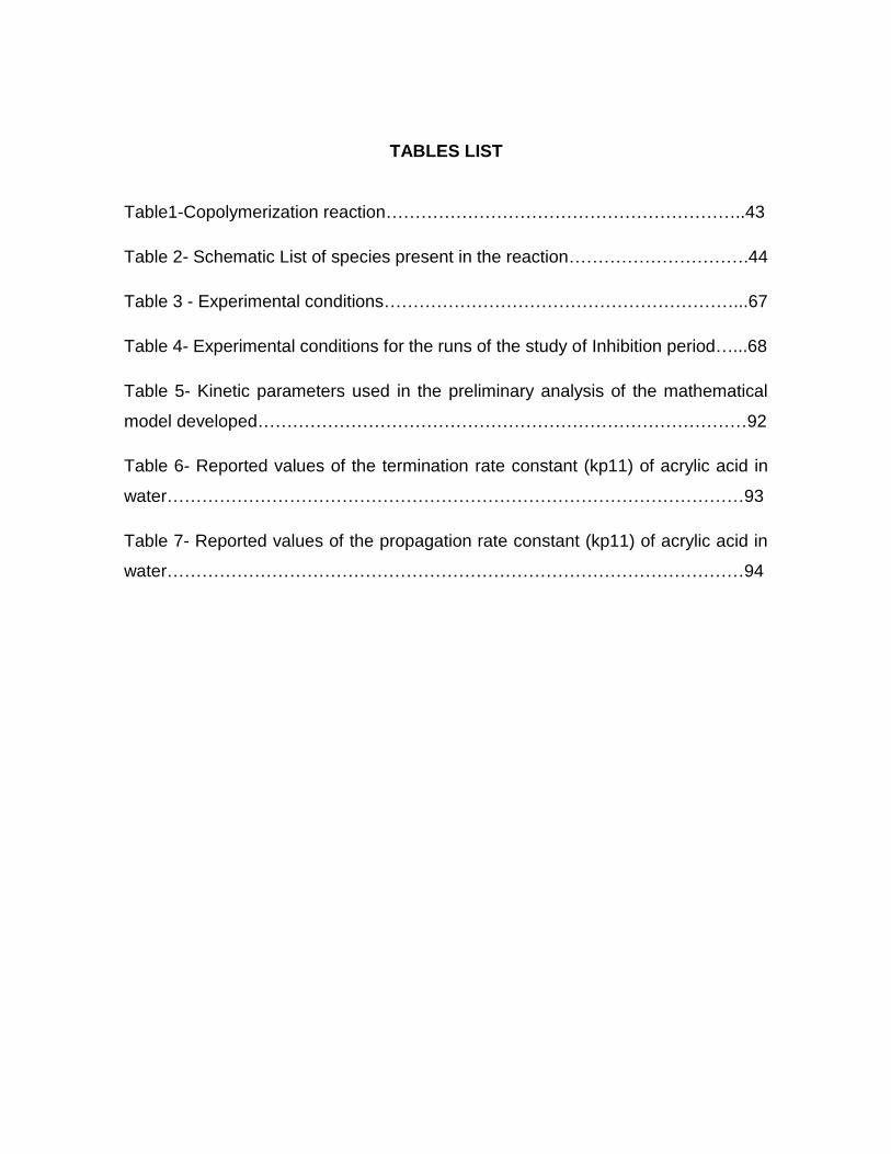
TABLES LIST

Table1-Copolymerization reaction……………………………………………………..43

Table 2- Schematic List of species present in the reaction………………………….44

Table 3 - Experimental conditions……………………………………………………...67

Table 4- Experimental conditions for the runs of the study of Inhibition period…...68

Table 5- Kinetic parameters used in the preliminary analysis of the mathematical

model developed…………………………………………………………………………92

Table 6- Reported values of the termination rate constant (kp11) of acrylic acid in

water………………………………………………………………………………………93

Table 7- Reported values of the propagation rate constant (kp11) of acrylic acid in

water………………………………………………………………………………………94

15

NOMENCLATURE AND SIGLE LIST

AA Acrylic acid

TMPTA Trimethylol propane triacrylate

PAA Poly(acrylic Acid)

PDB Pendent Double Bond

MWD Molecular Weight Distribution

ODE Ordinary Diferential Equation

TAO Tetraallyloxy ethane

EGDMA Ethylene glycol dimethylacrylate

FCC Free-radical crosslinking copolymerization

MEHQ Monomethyl ether of hydroquinone

MAA

PSSH

Methacrylic acid

Pseudo Steady State Hypothesis

16

SYMBOL LIST

I: Initiator;

Di: Pendant double bond;

PS: Dead Polymer containing "s" monomeric units;

Pr,i: Dead polymer containing pendant double bonds of type "i" and "r" monomeric

units;

R0: Primary Radical (formed by the initiator decomposition);

Mj: Monomer type j (j = 1: acrylic acid, j = 2: trimethylolpropane triacrylate);

Rr,i: Polymeric radical of size “r” and type "i" (i = 1: i = 2: i = 3: i = 4: i = 5);

S: Inert Species;

PH = Hydrogen Potential

kd: Rate constant for the initiator decomposition (s-1);

Ki,j: Rate constant of initiation of monomer or crosslinker agent (L.mol-1.s-1);

Kp,ij: Rate constant of propagation of a radical of the type "i" and a monomer of

type "j" (L.mol-1.s-1);

Kfr,i: Rate constant of chain transfer of a radical of the type "i" (L.mol-1.s-1);

kh: Rate constant of the hydrogen abstraction reaction (L.mol-1.s-1);

Ktc: Rate constant of termination by combination (L.mol-1.s-1)

Ktd: Rate constant of termination by disproportionation (L.mol-1.s-1);

KI: Constant initiation;

R0: Concentration of primary radicals;

M: Concentration monomer;

17

Kp: Constant propagation;

Y0: Moment of order zero for total radicals;

V: Volume of the reaction medium;

ρU: Density of the monomer unit (g/L);

ρM: Density of the monomer (g/L).

CI : molar concentration to Sodium Persulfate (moles/liter)

CM1 : molar concentration to Acrylic acid (moles/ml)

CM2: molar concentration to Trimethylolpropanetriacrylate (moles/liter)

CD3: molar concentration to Pendant double bond (moles/liter)

CD4: molar concentration to Pendant double bond (moles/liter)

qe : Feed Flow Rate (L/min)

m1 = weight of the empty Beaker flask (g),

m2 = weight of the flask with hydroquinone solution (g)

m3 = weight of the flask with the sample taken from the reactor plus HQ (g),

m4 = weight of the flask with the dry sample (g),

fhydroquinone = weight fraction of the hydroquinone solution added to the sample

fspan60 = weight fraction of Span 60 in the formulation,

facrylic acid = weight fraction of acrylic acid in the formulation.

m5 = weight of the empty filter paper (g),

m6 = weight of the initial dry polymer sample and the filter paper (g),

m7 = weight of the final dry sample after extraction and filter paper (g).

18

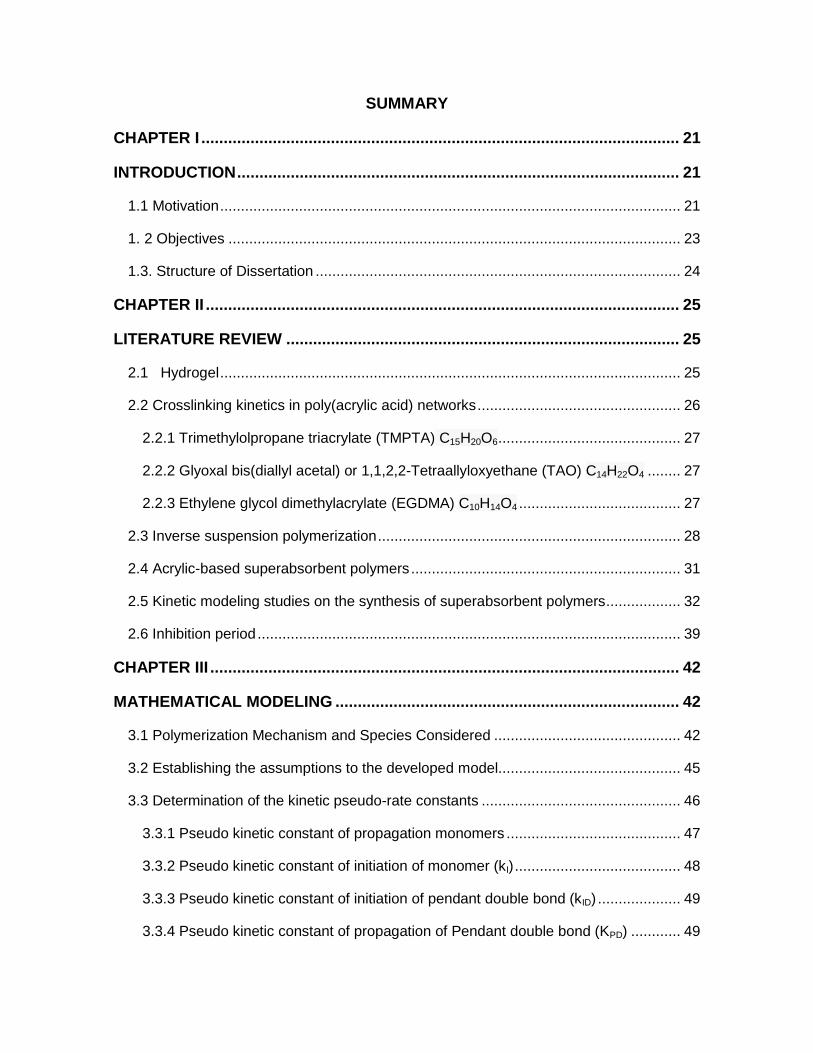
SUMMARY

CHAPTER I ........................................................................................................... 21

INTRODUCTION ................................................................................................... 21

1.1 Motivation ............................................................................................................... 21

1. 2 Objectives ............................................................................................................. 23

1.3. Structure of Dissertation ........................................................................................ 24

CHAPTER II .......................................................................................................... 25

LITERATURE REVIEW ........................................................................................ 25

2.1 Hydrogel ............................................................................................................... 25

2.2 Crosslinking kinetics in poly(acrylic acid) networks ................................................. 26

2.2.1 Trimethylolpropane triacrylate (TMPTA) C15H20O6 ............................................ 27

2.2.2 Glyoxal bis(diallyl acetal) or 1,1,2,2-Tetraallyloxyethane (TAO) C14H22O4 ........ 27

2.2.3 Ethylene glycol dimethylacrylate (EGDMA) C10H14O4 ....................................... 27

2.3 Inverse suspension polymerization ......................................................................... 28

2.4 Acrylic-based superabsorbent polymers ................................................................. 31

2.5 Kinetic modeling studies on the synthesis of superabsorbent polymers .................. 32

2.6 Inhibition period ...................................................................................................... 39

CHAPTER III ......................................................................................................... 42

MATHEMATICAL MODELING ............................................................................. 42

3.1 Polymerization Mechanism and Species Considered ............................................. 42

3.2 Establishing the assumptions to the developed model ............................................ 45

3.3 Determination of the kinetic pseudo-rate constants ................................................ 46

3.3.1 Pseudo kinetic constant of propagation monomers .......................................... 47

3.3.2 Pseudo kinetic constant of initiation of monomer (kI) ........................................ 48

3.3.3 Pseudo kinetic constant of initiation of pendant double bond (kID) .................... 49

3.3.4 Pseudo kinetic constant of propagation of Pendant double bond (KPD) ............ 49

19

3.3.5 Calculating the mole fraction of radicals of type “i” ........................................... 51

3.4 Model Description ................................................................................................. 53

3.4.1 Mass Balance .................................................................................................. 53

3.4.2 Balance of Moments ........................................................................................ 57

3.4.3 Numerical Fractionation Technique .................................................................. 60

CHAPTER IV ........................................................................................................ 66

EXPERIMENTAL SECTION ................................................................................. 66

4.1 Materials................................................................................................................. 66

4.2 Equipments ............................................................................................................ 68

4.3 Experimental Procedure: ........................................................................................ 69

4.3.1 Preparation of the organic phase ..................................................................... 69

4.3.2 Preparation of the aqueous phase ................................................................... 69

4.3.3 Polymerization runs ......................................................................................... 70

4.3.4 Purification monomer ....................................................................................... 70

4.3.5 Study of the inhibition period ............................................................................ 71

4.3.6 Gravimetric analysis for conversion.................................................................. 72

4.3.7 Determination of gel fraction by Soxhlet system ............................................... 74

CHAPTER V ......................................................................................................... 76

RESULTS AND DISCUSSIONS ........................................................................... 76

5.1 Conversion measured by Gravimetry ..................................................................... 76

5.1.2 Homopolymerization ........................................................................................ 76

5.1.3 Copolymerization ............................................................................................. 78

5.2 Gel Fraction ............................................................................................................ 89

5.2.1 Crosslinker agents ........................................................................................... 89

5.3. Simulation results and comparison with experimental data .................................... 92

5.3.1 Effect of the value of the propagation rate constant (kp11) ................................ 93

20

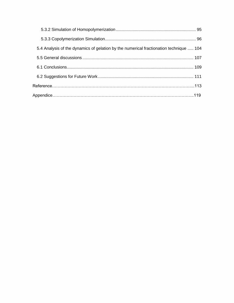
5.3.2 Simulation of Homopolymerization ................................................................... 95

5.3.3 Copolymerization Simulation ............................................................................ 96

5.4 Analysis of the dynamics of gelation by the numerical fractionation technique ..... 104

5.5 General discussions ............................................................................................. 107

6.1 Conclusions .......................................................................................................... 109

6.2 Suggestions for Future Work ................................................................................ 111

Reference………………………………………………………………………………………...113

Appendice………………………………………………………………………………………..119

21

CHAPTER I

INTRODUCTION

This chapter presents the general considerations and motivation for the

study, the objectives, and the structure of the dissertation.

1.1 Motivation

The synthesis and application of hydrogels have received special attention

of researchers in recent years.

Hydrogels are three-dimensional chains of hydrophilic polymers or

copolymers; despite their affinity for water, they are insoluble due to the presence

of crosslinking in their structure, which characterizes them as polymer networks.

Hydrogels have been used in the sanitary industry, agriculture, environment,

separation procedures and other operations of chemical engineering. They have

also been used in clinical practice and experimental medicine for a wide range of

applications, including tissue engineering and separation of biomolecules, among

others. However, the application that has raised more interest is the controlled

release of drugs.

The modeling of the hydrogels polymerization allows systematize the

knowledge of the reaction mechanism. The importance of developing the models

and improve the ability to predict, and therefore to control the reaction rates and

the molecular structure of the polymer formed, are key aspects in the design and

operation of polymerizing reactors.

In relation to mathematical modeling, currently there is a growing need for a

more detailed understanding of the phenomena taking place in the polymer

22

reactor. One quantitative form of this process understanding is the mathematical

model, which can represent the detailed behavior of the polymerization process.

The mathematical model is an invaluable tool for developing the optimal design

and optimal control system for these reactors.

The copolymerization with polyvinyl acrylic monomers in aqueous phase has

a complex kinetics that have been studied in recent years, the influence of factors

such as temperature and pH on the reaction rate of these chemical systems. Due

to lack of mechanistic understanding of this process, the literature still has little

information regarding the speed of the reactions involved in the polymerization of

hydrogels.

Suspension polymerization has been the focus of much attention due to its

easy temperature control, low viscosity of the dispersion, low levels of impurities

within the polymer product, and low separation cost, when compared with bulk and

solution polymerization processes.

The advances in industrial production of polymers occurred in an

accelerated manner. Synthetic polymers present advantages such as versatility in

terms of final properties (e.g., glass transition temperature and modulus of

elasticity), which can be modified in function of the process variables (e.g.,

concentration of reactants, additives and temperature). Many polymers are

produced and sold without a clear, detailed understanding on the polymer structure

or on the reactions involved in their synthesis. For instance, in the controlled

radical copolymerization process, some open questions are the need to define the

mechanism involved, the presence of secondary reactions; the effects caused by

the addition of controlling agent on the gel point and on the polymer properties

produced; the formation of cyclizations and their effects on the final product

properties.

In the present work, the production of hydrogels of poly (acrylic acid) was

experimentally studied using the inverse suspension polymerization process. The

present work contributes as an effort improve the understanding of the

23

polymerization process of the synthesis of hydrogels, by combine a set of

experiments and the interpretation of the results by a mathematical model of the

process.

In this work, a kinetic model based on population balance was developed to

simulate the inverse-suspension polymerization process for producing hydrogels of

acrylic acid and trimethylolpropane triacrylate. The experiments were carried out in

a semibatch mode with control of the process variables. The sensitivity of the

copolymerization of acrylic acid and trimethylolpropane triacrylate to the presence

of dissolved oxygen in the reaction medium was analyzed to verify possible action

as inhibitor or retardant of the polymerization.

The purpose of this study is to better understand the kinetic mechanism, to

evaluate kinetics parameters, as well as the effects of the operating conditions, for

example, temperature or reagent concentrations during the polymerization process

on the monomer conversion and gel fraction.

1. 2 Objectives

General objetive

To perform experiments of polymerization of acrylic acid / trimethylolpropane

triacrylate (TMPTA) and measure process variables such as monomer

conversion and gel fraction, modifying reagent concentrations of initiator and

crosslinking, and evaluating effects on the reaction to different operating

temperatures, feeding time, and presence/concentration of inhibitor.

Specific objectives

To identify the phenomena involved in the production process of the hydrogels

and interpret them in terms of the reaction mechanisms currently found in the

literature, thus contributing to a better understanding of the polymerization

24

process in terms of the fundaments (a mathematical model was used to assist

in this study);

To determinate the changes in gel fraction during the prolymerization process,

by using the extraction method, and from experimental data, to analyze the

evolution of the gel fraction using different number of generations in the

technique of numerical fractionation and considering different values of kinetic

constants;

To verify the effectiveness of the cross-linking agents trimethylolpropane

triacrylate (TMPTA), tetraallyloxyethane (TAO) and ethylenglicol dimetracrylate

(EGDMA) used in the experimental study and compare the gel formation in the

systems.

1.3. Structure of Dissertation

This dissertation is structured as described below.

In Chapter 2, a literature review on the subjects related to this work is

presented, emphasizing some recent work in the area. It also describes some

concepts that were used throughout the study.

Chapter 3 describes the mathematical model of the polymerization system

studied.

Chapter 4 presents the experimental equipment and the methods employed

in the experiments.

Chapter 5 presents the results of the experimental study, as well as, the

simulation results.

Finally, Chapter 6 presents conclusions and recommendations and

suggestions for further studies.

25

CHAPTER II

LITERATURE REVIEW

This Chapter presents general information taken from the literature about

the main topics treated in the dissertation. It includes the basic concepts about

hydrogels and inverse suspension polymerization. Also, a literature review is

presented on the different experimental studies and on the kinetic studies of

polymerization processes used to obtain hydrogels.

2.1 Hydrogel

Hydrogel products constitute a group of polymeric materials, the hydrophilic

structure of which renders them capable of holding, by swelling, large amounts of

water in their three-dimensional networks. Extensive use of these products in a

number of industrial and environmental areas of application is considered to be of

prime importance such as pharmaceutical, biology, separation process etc.

The materials of interest in this brief review are primarily hydrogels, which

are polymer networks extensively swollen with water.

Hydrogels can be divided into two categories based on the chemical or

physical nature of the cross-link junctions. Chemically cross-linked networks have

permanent bonds, while physical networks have nonpermanent connections that

arise from either polymer chain entanglements or physical interactions such as

ionic interactions, hydrogen bonds and dipole forces (Ahmed, 2013).

Hydrogels are usually prepared from polar monomers. According to their

starting materials, they can be divided into natural polymer hydrogels, synthetic

polymer hydrogels, and combinations of the two classes. From a preparative point

of view, they can be obtained by graft polymerization, cross-linking polymerization,

networks formation of water-soluble polymer, radiation-induced cross-linking, etc.

There are many types of hydrogels; mostly, they are slightly cross-linked

26

copolymers of acrylate and acrylic acid, and grafted starch-acrylic acid polymers

prepared by inverse suspension, emulsion polymerization, and solution

polymerization.

2.2 Crosslinking kinetics in poly(acrylic acid) networks

A cross-link is a bond that links one polymer chain to another. They can be

covalent bonds or ionic bonds. "Polymer chains" can refer to synthetic polymers or

natural polymers (such as proteins). When the term "cross-linking" is used in the

synthetic polymer science field, it usually refers to the use of cross-links to promote

a difference in the polymers' physical properties. When "crosslinking" is used in the

biological field, it refers to the use of a probe to link proteins together to check for

protein–protein interactions, as well as other creative cross-linking methodologies.

Cross-linking is used in both synthetic polymer chemistry and in the

biological sciences. Although the term is used to refer to the "linking of polymer

chains" for both sciences, the extent of crosslinking and specificities of the

crosslinking agents vary. When cross links are added to long rubber molecules, the

flexibility decreases, the hardness increases and the melting point increases as

well.

Network formation in free-radical polymerization is a non-equilibrium

process, namely, it is kinetically controlled, and therefore each primary polymer

molecule experiences a different history of crosslinking.

Different kind of crosslinker can be used in order to produce hydrogels; two

most used are trimethylolpropane triacrylate (TMPTA) and tetraallyloxyethane

(TAO) and ethylene glycol dimethylacrylate (EGDMA).

27

2.2.1 Trimethylolpropane triacrylate (TMPTA) C15H20O6

Trimethylolpropane triacrylate is a trifunctional monomer used in the

manufacture of plastics, adhesives, etc. It is useful for its low volatility and fast cure

response, and improves the properties of resistance against weather, chemical,

water and abrasion. End products include alkyd coatings, compact discs,

hardwood floors, concrete polymers, dental polymers, lithography, letterpress,

screen printing, elastomers, automobile headlamps, acrylics and plastic

components for the medical industry.

2.2.2 Glyoxal bis(diallyl acetal) or 1,1,2,2-Tetraallyloxyethane (TAO) C14H22O4

1,1,2,2-Tetraallyloxyethane is a tetrafunctional crosslinker used for different

applications; it has a high functionality due to the presence of the double bonds,

with variations in their reactivities. This crosslinking agent is used to prepare

superabsorbent, hydrophilic gels that are able to retain, at a high absorption rate,

huge amounts of water.

2.2.3 Ethylene glycol dimethylacrylate (EGDMA) C10H14O4

Ethylene glycol dimethylacrylate is a diester formed by condensation of two

equivalents of methacrylic acid and one equivalent of ethyleneglycol. EGDMA can

be used as crooslinker in free radical copolymerizations. When used with methyl

methacrylate, it leads to gel point at relatively low concentrations because of the

nearly equivalent reactivities of all the double bonds involved.

28

2.3 Inverse suspension polymerization

Dispersion polymerization is an advantageous method for preparing polymer

dispersions because the products are obtained as powder or microspheres

(beads), and thus, grinding is not required. In the production of hydrogels, water-in-

oil (W/O) process is chosen instead of the more common oil-in-water (O/W)

processes, and then the polymerization is referred to as „„inverse suspension

polymerization‟‟.

The dispersion is thermodynamically unstable and requires both continuous

agitation and addition of a lipophilic-balanced (HLB) suspending agent.

In suspension polymerization, the drops are stabilized against coalescence

by the addition of water-soluble polymers called stabilizers or protective colloids.

One of the commonly used stabilizers is Span 60 (Ahmed, 2013).

The function of surface-active agents is to absorb onto the droplet interface

and prevent other drops from approaching because of electrostatic and/or steric

repulsion forces. This causes a reduction of immediate coalescence due to the

increasing strength of the liquid film entrapped between two colliding drops. The

presence of a protective film prolongs the contact time required for drop

coalescence, thus, increasing the probability of drop separation by agitation

(Ahmed, 2013).

The use of inverse suspension polymerization is a development relatively

new. Inverse suspension polymerization is conducted by dispersing water-soluble

monomers in a continuous organic phase. Thermodynamically, the dispersion is

unstable and requires continuous stirring and adding of stabilizing agents. Initiation

(production of free radicals) is usually done thermally or chemically, with chemical

initiators such as azo-compounds or peroxide compounds. In the case of using a

single initiator component, polymerization may be initiated by decomposition of the

initiator in the organic phase, in the aqueous phase or in both phases, depending

29

on how the initiator is partitioned into the two phases (Machado; Lima; Pinto,

2007).

Kalfas et al. (1993) carried out extensive studies of aqueous suspension

homo- and copolymerizations with methyl methacrylate, styrene, and vinyl acetate

in a lab-scale batch reactor. Simulation results from homogeneous and two-phase

free-radical polymerization kinetic models, using physical and kinetic parameter

values taken from the literature of bulk and solution polymerization were found to

be in good agreement with batch suspension experimental results.

Wang et al. (1997) studied the synthesis of water-superabsorbent sodium

polyacrylate by inverse suspension polymerization, using Span60 as the

dispersant, cyclohexane as the organic phase, N,N*-methylene bisacrylamide as

the crosslinking agent, and potassium persulfate as the initiator. The effect of

reaction conditions such as reaction time, and concentrations of crosslinking agent,

and dispersant on the swelling of deionized-water and saline solution, average

particle size, and distribution of the sol–gel of the resin was discussed. The

deionized-water and saline-solution swelling ratios of sodium polyacrylate prepared

at proper conditions were 300–1200 and 50–120, respectively; the number-

average particle size was 10–50 mm and the weight fraction of gel was 20–85wt%.

Omidian et al. (1998) reported an exploratory investigation of the influence

of cross-linking agents on the capacity for absorbing water and on the rate of

absorption of acrylate polymers produced by using both inverse suspension and

solution polymerization, which are the main process used industrially. They used a

simple, small scale laboratory version of the polymerization part of this process,

which permitted contact with air and evaporative losses, the effects of varying the

heat input and the initiator concentration were explored. The presence of oxygen

resulted in an inhibition period which prolonged the time for completing

polymerization and consequently increased evaporative losses of water. The

swelling was highest for the products obtained under conditions of short reaction

times. Long reaction times resulted in long inhibition periods, runaway

30

polymerization and low swelling. These effects were accounted for in terms of

oxygen participation in the polymerization and extensive losses of water as the

solvent.

Mayoux et al. (2000) studied the crosslinked poly(acrylic acid) synthesized

by inverse suspension polymerization. This process was investigated to determine

the influence of different parameters like temperature, stirring speed, solution pH,

and crosslinker concentration and to obtain the best control of the kinetics. An

aqueous phase containing partially neutralized acrylic acid, crosslinking agent, and

initiator agent was dispersed in an organic phase and stabilized by a surfactant.

The inverse suspension was carried out in heptane as the organic phase with a

different ratio of neutralization of the monomer, different crosslinker concentrations,

and several stirring speeds. The polymerization was initiated by potassium

persulfate (K2S2O8) with N-N′-methylenebisacrylamide (MBAC) as the crosslinker

and sorbitan monooleate as the surfactant. The influence of several parameters on

the bead size and the swelling capacity was investigated. Particle diameters

ranged from 10 to 130 μm. The kinetic results obtained by differential scanning

calorimetry showed that conversion and polymerization rates are a function of the

solution pH, and they decreased when the concentration of the crosslinking agent

MBAC was higher than 7.5%.

Choudhary (2009) carried out inverse suspension polymerizations in a one-

liter glass reactor to produce superabsorbent polymers (SAPs) based on acrylic

monomers for hygiene applications. Strongly water-absorbing polymers, based on

acrylic acid, sodium acrylate were prepared by copolymerization using potassium

persulfate as initiator and N-N′ methylene-bisacrylamide (MBA) as crosslinking

agent. The effect of varying monomer, crosslinker, initiator, dispersant

concentration, reaction time and degree of neutralization, on absorption capacities

was investigated. The continuous hydrocarbon phase was taken as 50:50 wt%

mixture of n-heptane and cyclohexane (aliphatic-alicyclic) because the availability

of crosslinker in the aqueous phase is controlled by the partition coefficient of the

31

crosslinker between the aqueous phase and the continuous hydrocarbon phase.

The SAPs were evaluated for their free absorption capacities in distilled water,

saline solution (0.9wt% NaCl), and also absorption under load (AUL). The

experimental results show that these SAPs have good absorbency both in water

and in NaCl solutions. It was observed that SAP synthesized from acrylic acid with

about 70% degree of neutralization, containing 1wt% cross-linker, and 0.5–1.0wt%

initiator concentration with 10wt% dispersant exhibited absorption capacities in

water, saline solution as 220 g/g, 70 g/g, respectively.

2.4 Acrylic-based superabsorbent polymers

From a material resource point of view, superabsorbent polymers (SAPs)

can also be divided into natural macromolecules, semi-synthetic polymers, and

synthetic polymers. From a preparation point of view, they can be synthesized by

graft polymerization, cross-linking polymerization, networks formation of water-

soluble polymer and radiation cross-linking, etc. There are many types of SAPs

presently in the market, mostly they are lightly cross-linked copolymers of acrylate

and acrylic acid and grafted starch-acrylic acid polymers prepared by inverse

suspension, emulsion polymerization, and solution polymerization. There are some

examples of different studies.

Cutié et al. (1997) described the simplest polymerization kinetic model,

which has a first-order dependence in monomer and half order in initiator. The

isothermal polymerization (55°C), of acrylic acid in water was monitored as a

function of concentration, degree of neutralization and initiator level to define a

kinetic model and to obtain accurate values for the rate constants.

The thesis of Souza (2013) focused on the experimental study of the

synthesis of hydrogels of poly(acrylic acid), as well as its mathematical

representation by building a kinetic model. For this purpose, experiments of acrylic

32

acid homopolymerization and copolymerization of acrylic acid and trimethylpropane

triacrylate in aqueous solution using sodium persulfate as initiator were performed.

Conversion, gel fraction and quantification of pendant double bonds were

determined using gravimetric techniques, extraction with water and titration

respectively. A mathematical model was developed, in order to achieve a better

understanding of the process.

2.5 Kinetic modeling studies on the synthesis of superabsorbent polymers

Few recent studies were found in the literature on kinetic modeling of the

reaction of inverse suspension polymerization for producing hydrogels.

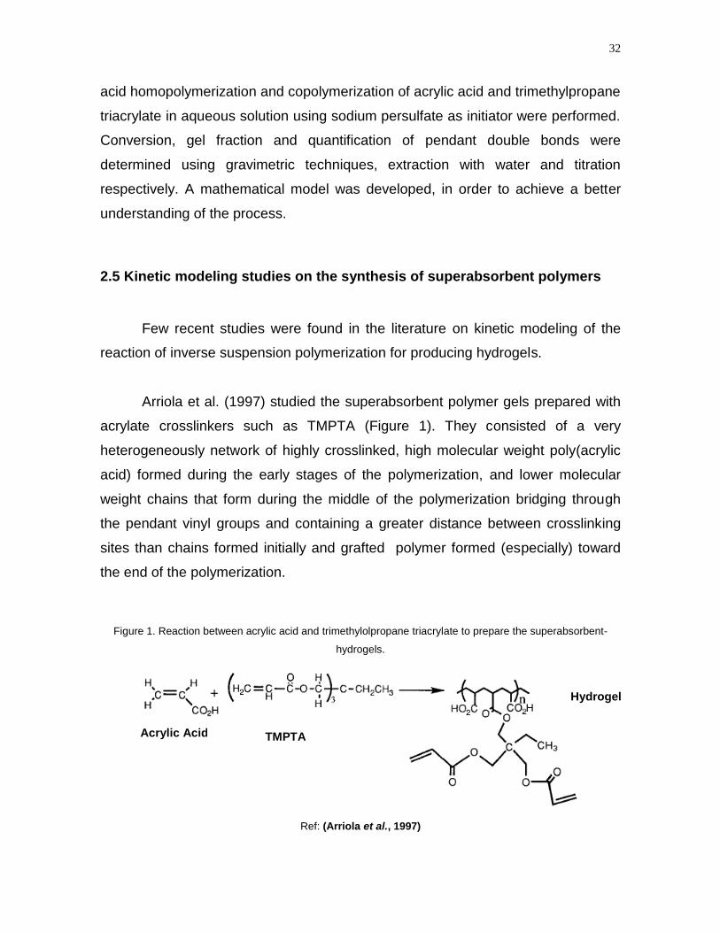
Arriola et al. (1997) studied the superabsorbent polymer gels prepared with

acrylate crosslinkers such as TMPTA (Figure 1). They consisted of a very

heterogeneously network of highly crosslinked, high molecular weight poly(acrylic

acid) formed during the early stages of the polymerization, and lower molecular

weight chains that form during the middle of the polymerization bridging through

the pendant vinyl groups and containing a greater distance between crosslinking

sites than chains formed initially and grafted polymer formed (especially) toward

the end of the polymerization.

Figure 1. Reaction between acrylic acid and trimethylolpropane triacrylate to prepare the superabsorbent-

hydrogels.

Ref: (Arriola et al., 1997)

Acrylic Acid

TMPTA

Hydrogel

33

Arriola et al. (1997) evaluated the reactivity ratio for acrylic acid, varied from 0.31

(65% neutralization) to 0.77 (non-neutralized). The reactivity ratio was affected by

the percent solids (solvent effect), but was insensitive to temperature over the

range of 55–80°C. It was observed that all of the double bonds of TMPTA were

incorporated into gel network as opposed to prior models predicting only two bonds

reacting. The reported inefficiency of TMPTA is postulated to be caused by a

solubility problem in the monomer mixture. Very low levels of extractables were

found in the products even though the crosslinker was consumed by 70%

conversion. Based on these data, they proposed that a major component of the gel

network is graft polymer that forms late in the polymerization onto the crosslinked

gel formed earlier.

Cutie et al. (1997) used nuclear magnetic resonance (NMR) to monitor the

polymerization rates in situ. This method made it possible to obtain isothermal data

during exothermic conditions of up to 2% conversion/min in 5 mm tubes. The 5 mm

diameter NMR tubes were loaded via a glass pipette and deoxygenated with

nitrogen. The results showed that the rate of incorporation of the crosslinker

(TMPTA) was, under all conditions, much faster than the rate of polymerization of

acrylic acid, the rate of incorporation of crosslinker resulting in earlier depletion

from the monomer mixture, was faster in the more neutralized systems.

McKenna et al. (2000) investigated the inverse suspension of partially

neutralized acrylic acid under variations of initiator and surfactant concentrations;

they used data taken at low initiator concentration and maximum stirring rate to

evaluated some kinetic constants and compared with literature values.

Costa et al. (2003) presented a kinetic approach for modeling irreversible

non-linear polymerizations. Their model utilizes the numerical fractionation

technique and is capable of predicting a broad range of distributional properties

both for pre- and postgel operating conditions as well as polymer properties such

34

as the crosslink density and branching frequency. Mass balance equations in terms

of the moment generating function of the distribution of mole concentrations of

polymeric species for free radical copolymerizations of mono/divinyl monomers

could be numerically solved after gel point. They observed that the predictions by

the pseudo-kinetic method are reasonable only when equal reactivity of double

bonds prevails, causing early gelation in the batch reactor. The mathematical

model for the crosslinking copolymerization of a vinyl and a divinyl monomer was

developed and applied to the case of polymerization of methyl methacrylate and

ethylene glycol dimethacrylate in a batch reactor. Model results compared

favorably to the experimental data of Li et al. (1989) for the system investigated

and confirmed the experimental findings of Li et al. (1989) that either the increase

of CTA concentration or the decrease of divinyl monomer delays the onset of

gelation. The effects of these variables on the crosslink densities are also

demonstrated using this model. After gelation, the decrease in sol crosslink density

is faster at higher levels of divinyl monomer, while gels of higher crosslink densities

are obtained at higher levels of divinyl monomer.

Harrisson et al. (2003) evaluated the rate constants of propagation and

termination of methyl methacrylate (MMA) in the ionic liquid 1-butyl-3-

methylimidazolium hexafluorophosphate using the pulsed laser polymerization

technique across a range of temperatures. Arrhenius parameters were calculated

for the rate of propagation at ionic liquid concentrations of 0, 20, and 50% v/v. The

decrease in activation energy leads to large increases in the rate of propagation. In

addition, the rate of termination decreases by an order of magnitude as the ionic

liquid concentration is increased to 60% v/v. The increase in propagation rate was

attributed to the increased polarity of the medium, while the decrease in the

termination rate is due to its increased viscosity.

Rintoul et al. (2005) studied the reactivity ratio of polar monomers such as

acrylic acid in free radical copolymerization. A strong impact on the reactivity ratios

were identified for the pH and total monomer concentration. Specifically, at

35

constant total monomer concentration of 0.4 mol/L and T=313 K, the reactivity ratio

of acrylamide increases from 0.54 at pH 1.8 to 3.04 at pH 12. Contrarily, the

reactivity ratio of acrylic acid decreases from 1.48 to 0.32. Electrostatic effects to

the variation of the degree of ionization of acrylic acid were primarily suggested to

influence the kinetics. When the total monomer concentration increases from 0.2 to

0.6 mol/L at constant pH=12, the reactivity ratios of acrylamide and acrylic acid

decrease from 4.01 to 2.13 and increase from 0.25 to 0.47, respectively. Reduction

of electrostatic repulsion between the ionized monomer acrylic acid and partially

charged growing polymer chain ends due to higher ionic strength at higher total

monomer concentration serves as explanation of the effect.

The thesis of Haque (2010) presented an experimental investigation

performed to study the kinetics of copolymerization of monomers in aqueous and

alcoholic media by considering factors such as type of initiator and solvent, and

pH, in order to determine how these affect the reactivity ratios of these monomers.

Reactivity ratios were determined by non-linear least squares (NLLS) and the

error-in-variables-model (EVM) techniques and full conversion range kinetic

investigations were carried out to confirm these values.

Gonçalves et al. (2011) presented a kinetic model for gelling free radical

polymerization based upon population balance equations of generating functions,

and applied this model to predict the variations, in a batch reactor, of properties

such as the weight fraction of gel and the average molecular weights of the soluble

fraction. Simulations were carried out considering the synthesis of polyacrylic acid

gels with a trifunctional crosslinker (TMPTA used as case study) at an initial mole

fraction in the monomer mixture of 0.0025% (around the lower limit used in

practice). In these simulations, three different values of the rate coefficient for the

homopropagation of acrylic acid (kp1) were considered, in a range that is plausible

for this monomer under these particular conditions. Predictions were used to

evaluate the dependence of the dynamics of gelation on the following

kinetic/operation parameters:

36

Propagation rate coefficient of monovinyl monomer (acrylic acid);

Reactivity ratio of the pendant double bonds of the crosslinker;

Initial mole fraction of the crosslinker;

Functionality of the crosslinker (bi-, triand, tetrafuncional were considered).

Kinetic parameters (propagation and termination rate coefficients) for this

copolymerization system varies with different synthesis conditions (temperature,

concentration, pH, ionic strength, etc), showing the following effects:

- Monomer/solvent concentration ratio with non-ionic systems. A decrease of

about one order of magnitude in kp was observed upon increasing monomer

concentration.

- Degree of ionization. At low monomer concentration, a decrease in kp of

about one order of magnitude was measured when the degree of ionization

was changed from 0 to 100%.

- Opposite variations were observed when the two effects (monomer

concentration and ionization) are present: a weaker drop of kp with

monomer concentration was found when the monomer is partially ionized.

For a fully ionized monomer, kp increases when monomer concentration is

also increased. Occurrence of Trommsdorff effect is another issue

complicating the kinetics of these polymerization systems.

The above observations show that is difficult to establish a fully reliable set of

kinetic parameters valid for the different conditions to be considered in the

synthesis of water soluble homopolymers based on acrylic acid.

Simulations like those presented in Figure 2 and Figure 3 can be used to

estimate the reactivity of PDBs using experimental measurements of the dynamics

of gel formation. The effect of the initial mole fraction of crosslinker (Yc) on the

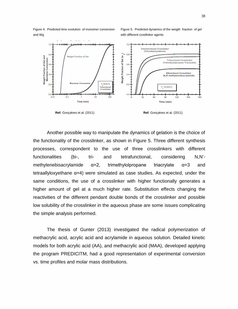
dynamics of the weight fraction of gel is illustrated in Figure 4. This variable can be

readily used to manipulate the properties of the final products, as depicted in that

figure. Simulations for Yc ranging from the lower limit used in practice (around

0.0025%) to ten times this value show the change of Wg from around 0.4 to 1.

37

Under these conditions, gelation is predicted to occur within some

hundredths of seconds as shown in Figure 4 and the weight fraction of gel in the

polymer rises very fast to around 1. However, in practice, polymerization must be

prolonged in order to reach high monomer conversion.

Kinetic gelation theories are able to deal with spatial heterogeneities

resulting from topological constraints occurring with highly crosslinked networks but

on the other hand present deficiencies with lightly crosslinked systems due to the

failure to account for monomer and polymer mobility.

Figure 2. Predicted dynamics of the weight fraction of gel

(wg) and monomer conversion. Effect of reactivity of the

pendant double bonds

Figure 3. Predicted dynamics of the weigth fraction of gel

(wg). Effect of the initial mole fraction of crosslinker.

Ref: Gonçalves et al. (2011)

38

Figure 4. Predicted time evolution of monomer conversion

and Wg

Figure 5. Predicted dynamics of the weigth fraction of gel

with different crosllinker agents

Ref: Gonçalves et al. (2011)

Ref: Gonçalves et al. (2011)

Another possible way to manipulate the dynamics of gelation is the choice of

the functionality of the crosslinker, as shown in Figure 5. Three different synthesis

processes, correspondent to the use of three crosslinkers with different

functionalities (bi-, tri- and tetrafunctional, considering N,N‟-

methylenebisacrylamide α=2, trimethylolpropane triacrylate α=3 and

tetraallyloxyethane α=4) were simulated as case studies. As expected, under the

same conditions, the use of a crosslinker with higher functionally generates a

higher amount of gel at a much higher rate. Substitution effects changing the

reactivities of the different pendant double bonds of the crosslinker and possible

low solubility of the crosslinker in the aqueous phase are some issues complicating

the simple analysis performed.

The thesis of Gunter (2013) investigated the radical polymerization of

methacrylic acid, acrylic acid and acrylamide in aqueous solution. Detailed kinetic

models for both acrylic acid (AA), and methacrylic acid (MAA), developed applying

the program PREDICITM, had a good representation of experimental conversion

vs. time profiles and molar mass distributions.

39

2.6 Inhibition period

Substances that may be present in the polymerization medium in very small

quantities, causing a large decrease in the polymerization rate can be classified

into two types according to their effectiveness: inhibitors and retarders. Inhibitors

neutralize all free radicals, those come from the initiator, of the active centers of the

chains or from the monomer. The polymerization is complete standstill until the

inhibitor is consumed. Retardants are less effective inhibitors and neutralize only a

fraction of the radicals. In this case, polymerization can occur, but at a slower

speed. Some authors relate the mechanism responsible for inhibiting the

deactivation of the centers of initiation or reduction in the rate of generation of

these, while the delay associated with the interruption of chain propagation

(Bamford, 1988). Same substance can act as an inhibitor, retarder or both

simultaneously, depending on its concentration. The difference between inhibitors

and retarders is therefore in magnitude, not as to the way in which the inhibition or

delay occurs.

Cutie et al. (1997) studied the effect of the monomethyl ether of

hydroquinone (MEHQ) on the polymerization of acrylic acid. The rate of

polymerization was quantified at various levels of MEHQ by use of an in situ NMR

technique. While oxygen acts as an inhibitor in acrylic acid polymerizations, MEHQ

was shown to function as a retarder. The decrease in the rate of polymerization

allowed the calculation of an inhibition constant for this system. MEHQ was found

to remain in the polymerizing mixture throughout the course of the reaction,

significantly reducing the rate of polymerization, but not reducing the molecular

weight of the polymer.

Bunyakan et al. (1999) evaluated the isothermal acrylic acid polymerization

by precipitation in toluene at various monomer and initiator concentrations over the

temperature range of 40°C–50°C. 2,2-Azobis (2,4-dimethyl-valeronitrile) was

employed as a chemical initiator. The rate of polymerization was found to depend

40

on the monomer and initiator concentration to the 1.7th and 0.6th orders,

respectively. The greater than first order dependence on monomer concentration

indicates a secondary, monomer-enhanced, decomposition step for the initiator

molecules. The approximately half-order dependence of the rate of precipitation

polymerization on the initiator concentration indicates that the chain termination

process is predominantly bimolecular.

Li et al. (2006) studied the inhibitors MEHQ (monomethyl ether

hydroquinone) and PTZ (phenothiazine) that are added to commercial acrylic acid

to prevent its spontaneous polymerization during shipping and storage. Dissolved

oxygen is also an strong inhibitor, and its presence in the solution enhances the

inhibition effects of MEHQ. The authors developed a comprehensive mathematic

model for the inhibition of acrylic acid polymerization and simulated the inhibition

effects of oxygen and MEHQ on the polymerization of acrylic acid in batch and

semi-batch processes. The key kinetic parameters were obtained from the

literature or estimated from experimental data in the literature. The model was able

to predict most of the effects of inhibitors. Although the literature data used did not

show the synergistic inhibition effects of oxygen and MEHQ, the model was able to

predict the effects. Simulation results showed that oxygen is a strong inhibitor in

both batch and semi-batch reactors and does not act as a retarder as expected.

Lorber et al. (2010) presented an original tool to monitor polymerization

kinetics. It consists in a droplet based millifluidic approach where the use of

aqueous droplets of monomer can be seen as polymerization microreactors.

Acrylic acid mixed with sodium persulfate at low pH was used as a fast and

exothermic polymerization model. By using a nonintrusive spectroscopic system

with a millifluidic system, they were able to safely investigate harsh polymerization

conditions. As expected, polymerizations exhibited higher order with respect to

monomer concentration than the usual first-order kinetics expected for ideal free-

radical polymerization, and half-order dependence with respect to the initiator

concentration. These results indicated the potential for further studies of

41

polymerization reactions where detailed basic kinetic data must be acquired in

conditions which cannot be investigated by using conventional batch glassware,

i.e., high temperatures or concentrations. This versatile approach can also be used

as an efficient high throughput screening tool.

42

CHAPTER III

MATHEMATICAL MODELING

This Chapter presents the mathematical model used to interpret the

experimental results of this dissertation for inverse-suspension polymerization of

acrylic acid and trimethylolpropane triacrylate (TMPTA), a crosslinker with

functionality 3 (number of active double bonds). This model was based on that

developed in the thesis of Aguiar (2013) and also used in the work of Souza

(2013).

3.1 Polymerization Mechanism and Species Considered

The mathematical model was developed in this research using the

population balance for the different species present in the reactor.

The species considered are the following:

I: Initiator;

Di: Pendant double bond type i;

PS: Dead Polymer containing "s" monomeric units;

Pr,i: Dead polymer containing pendant double bonds of type "i" and "r" monomeric

units;

R0: Primary Radical (formed by the initiator decomposition);

Mj: Monomer type j (j = 1: acrylic acid, j = 2: trimethylolpropane triacrylate);

Rr,i: Polymeric radical of size “r” and type "i" (i = 1: i = 2: i = 3: i = 4: i = 5);

S: Inert Species;

43

Table 1 shows the reaction steps considered in the mechanism:

decomposition of the initiator, initiation, propagation and termination of the chains,

chain transfer to the polymer and the hydrogen abstraction. The kinetic scheme

presented in Table 1 is a simplified description of the polymerization system that

was here adopted in order to keep this presentation within a manageable size;

however, this kinetic approach was conceived to deal with much more detailed

descriptions of non-linear polymerization systems.

Table 1. Copolymerization reaction

Reaction Mechanism

Initiator Thermal Decomposition 02RI dk

Initiator 21 ,10 jRMR j

k

jIj

Monomer Propagation

21 ,51 ,1,, jiRMR jr

k

jirijp

Crosslinker Initiator

43 ,0, iRDR ir

k

iiI

PDB Propagation (crosslinking) 43 51 ,1, ijRDR jr

k

ijrpij

Hydrogen Abstration SRRP s

k

sh 0

Chain Transfer 51 ,,, iPRRP irs

k

irsifr

Termination by combination 51 51 ,, ijPRR sr

k

isjrtc

Termination by disproportionation

51 51 ,, ijPPRR sr

k

isjrtd

kd: Rate constant for the initiator decomposition (s-1);

ki,j: Rate constant of initiation of monomer or crosslinker agent (L.mol-1.s-1);

kp,ij: Rate constant of propagation of a radical of the type "i" and a monomer of type "j" (L.mol-1.s-1);

kfr,i: Rate constant of chain transfer of a radical of the type "i" (L.mol-1.s-1);

kh: Rate constant of the hydrogen abstraction reaction (L.mol-1.s-1);

ktc: Rate constant of termination by combination (L.mol-1.s-1)

ktd: Rate constant of termination by disproportionation (L.mol-1.s-1);

44

Table 2 presents a description of the different species, groups, radicals, monomers

and pendant double bonds considered in the model.

Table 2 - Schematic list of species considered in the model.

Symbol Name Species and group

I Initiator -

R0 Primary radical -

M1 Acrylic Acid

M2 TMPTA (Trimethylolpropanetriacrylate)

D3

Pendant double bond (PBDs)

D4 Pendant double bond (PBDs)

U1 Polymeric units AA ( acrylic acid)

U2

Polymeric unit AA (Acrylic Acid)

R1 Radical AA (Acrylic Acid)

R2 Radical TMPTA

(trimethylolpropanetriacrylate)

R3 Radical D3

R4 Radical D4

R5 Backbone radical

Source:(Souza, 2013)

45

3.2 Establishing the assumptions to the developed model

The following simplifying assumptions were considered in the development

of the kinetic model:

a) Pseudo Steady State Hypothesis (PSSH) for the radical species (i.e., the

radicals are considered to be consumed almost instantly after they are

produced, because of their very short lifetime; the net production rate of each

radical species is nil);

b) Pseudo-homopolymerization approach (the kinetics of the copolymerization

reactions are combined in proportion to the respective radical types and

monomer types);

c) Each soluble polymer chain has only one radical center (mono-radical);

d) The closure equation of Saidel and Katz (Aguiar et al., 2014) was used to close

the set of balance equations for the moments of the molecular weight

distribution;

e) During each time integration step, fractions of each type of radical are

considered to be constant. The rate of bimolecular reactions involving polymeric

groups is independent of the size of the polymer chain;

f) The reactions occur only in droplets dispersed in the organic medium (the

droplets behave or operate as a reactor); each monomer drop is considered as

a mini-reactor in which a bulk polymerization takes place and the overall

behavior of the reactor is the sum of every drop of behavior;

g) The drop density is constant (there are only changes in the volume during the

feed of the aqueous phase in the polymerization process);

h) Negligible cyclization reactions (this assumption was adopted because the

experimental quantification of the amount of double bonds for this systems is

not easy)

46

3.3 Determination of the kinetic pseudo-rate constants

Based on the assumptions and reaction mechanism for the polymerization

of acrylic acid and TMPTA, two monomer species are considered, five types of

polymeric radicals and two types of pendant double bonds, as shown in Table 2. In

order to simplify the model equations for this reaction scheme, the assumption of

pseudo-homopolymerization was adopted to determine the pseudo kinetic

constants. These constants were determined for the reactions of initiation and

propagation of monomers and pendant double bonds (Souza, 2013).

The mole fractions of the different radical types, of different monomer types, and of

different pendant double bonds are defined, respectively, as:

5

iRï

jj

Rf

R

(1)

1 2

iMi

Mf

M M

(2)

i

Di

Df

D

(3)

3 4

1

S

D Df

Q

(4)

1 2M M M (5)

3 4D D D (6)

47

1 1 2 2 1 211 12 21 22p p p p p

R M M R M Mk k k k k

R M M R M M

4 1 2 5 1 241 42 51 52p p p p

R M M R M Mk k k k

R M M R M M

3.3.1 Pseudo kinetic constant of propagation monomers

Considering the reaction scheme given in Table 1, the propagation rate is

expressed by:

1 11 1 12 2 2 21 1 22 2 3 31 1 32 2p p p p p p pR R k M k M R k M k M R k M k M

4 41 1 42 2 5 51 1 52 2p p p pR k M k M R k M k M (7)

For a homopolymerization, the propagation rate would be:

p pR k RM (8)

where R is the total radical concentration, while M is the total monomer

concentration. Substituting Equation 7 into 8:

1 11 1 12 2 2 21 1 22 2 3 31 1 32 2p p p p p pk RM R k M k M R k M k M R k M k M

4 41 1 42 2 5 51 1 52 2p p p pR k M k M R k M k M (9)

Dividing both sides by [R] [M]:

M

Mk

M

Mk

R

Rpp

232

131

3

1 11 1 12 2 2 21 1 22 2 3 31 1 32 2p R p M p M R p M p M R p M p Mk f k f k f f k f k f f k f k f

4 41 1 42 2 5 51 1 52 2R p M p M R p M p Mf k f k f f k f k f (10)

48

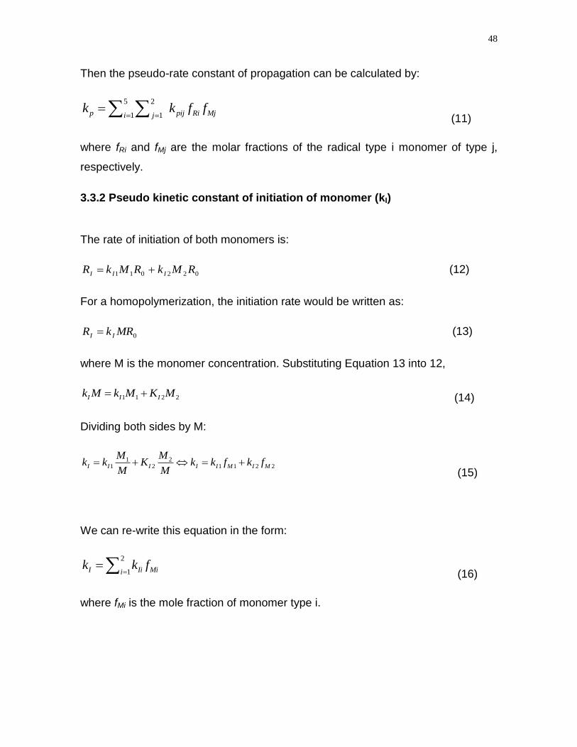
Then the pseudo-rate constant of propagation can be calculated by:

5 2

1 1p pij Ri Mji jk k f f

(11)

where fRi and fMj are the molar fractions of the radical type i monomer of type j,

respectively.

3.3.2 Pseudo kinetic constant of initiation of monomer (kI)

The rate of initiation of both monomers is:

022011 RMkRMkR III (12)

For a homopolymerization, the initiation rate would be written as:

0MRkR II (13)

where M is the monomer concentration. Substituting Equation 13 into 12,

1 1 2 2I I Ik M k M K M (14)

Dividing both sides by M:

1 21 2 1 1 2 2I I I I I M I M

M Mk k K k k f k f

M M

(15)

We can re-write this equation in the form:

2

1I Ii Miik k f

(16)

where fMi is the mole fraction of monomer type i.

49

3.3.3 Pseudo kinetic constant of initiation of pendant double bond (kID)

The rate of initiation of pending double bonds is expressed by:

3 0 3 4 0 4ID ID IDR k R D K R D (17)

For a homopolymerization, the corresponding herefore, the initiation

homopolymerization rate, for pendant double bond would be:

10QRkR IDIR (18)

Where D is the concentration of pendant double bond. Substituting Equation 18 in

17,

0 1 3 0 3 4 0 4ID ID IDk R Q k R D k R D (19)

Dividing both sides by R0 and (D3 + D4)

31 4

3 4 3 3 4 4

3 4 3 4 3 4

1ID ID ID ID ID D ID D

s

DQ Dk k k k k f k f

D D D D D D f

3 3 4 4ID ID D ID D sk k f k f f (20)

This equation can written as:

4

3ID IDi Di sik k f f

(21)

where is the molar pending i.e., the double type is the molar fraction of pending

double bond, the dead polymer fraction.

3.3.4 Pseudo kinetic constant of propagation of Pendant double bond (KPD)

The propagation rate of the pendant double bonds is expressed as:

50

1 13 3 14 4 2 23 3 24 4 3 33 3 34 4PD p p p p p pR R k D k D R k D k D R k D k D

4 43 3 44 4 5 53 3 54 4p p p pR k D k D R k D k D (22)

While for a homopolymerization, the corresponding rate would be:

1PD PD rR k R Q (23)

where in Rr represents the concentration of radicals size "r" while Q1 is the number

of monomeric units in neutral polymer. Substituting Equation 23 into 22:

)()(

)()()(

45435354443434

4343333424323241431311

5

1

DkDkRDkDkR

DkDkRDkDkRDkDkRQRk

pppp

ppppppr rPD

(24)

Dividing both sides by

5

1r rR e :43 DD

43

4

54

43

3

535

1

5

43

4

44

43

4

435

1

4

43

4

34

43

3

335

1

3

43

4

24

43

3

235

1

2

43

4

14

43

3

135

1

1

43

1

DD

Dk

DD

Dk

R

R

DD

Dk

DD

Dk

R

R

DD

Dk

DD

Dk

R

R

DD

Dk

DD

Dk

R

R

DD

Dk

DD

Dk

R

R

DD

Qk

pp

r r

pp

r r

pp

r r

pp

r r

pp

r r

PD

45435354443434

434333342432324143131'

1

DpDpRDpDpR

DpDpRDpDpRDpDpR

D

PD

fkfkffkfkf

fkfkffkfkffkfkff

k

D

DpDpRDpDpR

DpDpRDpDpRDpDpR

PD ffkfkffkfkf

fkfkffkfkffkfkfk '

45435354443434

434333342432324143131

(25)

51

5 4

12 1 2 1 1 11 1 1 1 1 1 1 12 30 p pi i p p i i fri i

k R M k R M k R M k R D k Q R

Simplifying the equation:

5

1 4433 'r DDpiDpiRiPD ffkfkfk (26)

where fRi and fDj are, respectively, the mole fractions of the polymeric radical of

type “i” and the mole fraction of double bonds of type “j”.

3.3.5 Calculating the mole fraction of radicals of type “i”

From a system of linear equations arising from the mass balance conducted for

each group, it is possible to determine the fraction of radicals of type "i". Ortiz

(2008) (apud Souza, 2013) disclosed a similar study using two types of radicals,

which results in a less complex solution to the system of equations.

The mass balance for the polymer type groups R1 is expressed below

5 41

1 0 1 12 1 2 1 1 11 1 1 1 12 3I p pi i p p i ii i

dRk R M k R M k R M k R M k R D

dt

5

1 1 1 11fr t jjk Q R k R R

(27)

According to the pseudo-steady state:

(28)

Dividing both sides of the equation 28, is obtained:

5 41 2 1 1

12 1 15 5 52 3

1 1

0 i i

p pi p ii i

j j jj j j

R M R M R Dk k k

M D M D M DR R R

52

1

1 5

1

fr

jj

R Qk

M DR

(29)

and,

5

1j j

iRi

R

Rf

DM

Mf i

i

' , for 2i

DM

Df i

i

' , for 43 i

DM

Qf S

1'

sRfrr RiPiRPr RiPiRP ffkffkffkffkffk '''''0 11

4

3 111111

5

2 112112 (30)

Developing the above equation, to obtain:

51541431321211

4

3 112121 ''''0 pRpRpRpRSfri ipPR kfkfkfkfffkfkfkf (31)

Following the same reasoning for the other extreme, one obtains the following

equations

2 21 2 23 3 24 4 2 2 1 12 3 32 4 42 5 520 ' ' ' 'R p p p fr S R p R p R p R pf k f k f k f k f M f k f k f k f k (32)

3 31 1 32 2 34 4 3 3 1 13 2 32 4 43 5 530 ' ' ' ' 'R p p p fr S R p R p R p R pf k f k f k f k f f f k f k f k f k (33)

4 41 1 42 2 43 3 4 1 4 1 14 2 24 3 34 5 540 ' ' 'R p p p fr R p R p R p R pf k f k f k f k Q D f k f k f k f k (34)

5 51 1 52 2 53 3 54 4 1 1 1 2 2 3 3 4 40 R p p p p R fr R fr R fr R frf k M k M k D k D Q f k f k f k f k (35)

1 2 3 4 51 R R R R Rf f f f f (36)

53

Fractions fi of each radical are obtained by solving the system of linear

equations (31) - (36). These fractions will be useful in the determination of pseudo-

kinetic constants.

3.4 Model Description

3.4.1 Mass Balance

Besides the differential equation of the balances of initiator, monomer A and

monomer B, the model has a set of ordinary differential equations for the balances

of radicals and dead chains of each size (population balance for the MWD).

The balances were formulated according to the reaction scheme

(mechanism) shown in Table 1 that takes into account the classical steps of free

radical polymerization in a batch reactor. (Figure 6).

Figure 6. Inverse suspension polymerization in a batch reactor

A B C

Ref.( Olivo 2015)

A : Organic Phase ( Toluene and Span 60)

B: Aquouse Phase ( Acrylic acid, tmpta, water and Sodium Persulfate)

A

A

54

Molar Balances of non-polymeric species

The mole balance in the semi-batch reactor for the non-polymeric molecular

species, for monomers and polymeric groups present have the following

expressions:

Initiator

VCKCq

dt

VCd

dt

dNIdIe

II

e (37)

Primary Radical

VQRkDRkMRkIfk

dt

VCd

dt

dNRhi iIij jIjd

R

10

4

3 0

2

1 00 20

(38)

Acrylic acid -M1

VMRkMRkCq

dt

VCd

dt

dNMi irr piIMe

M

5

1 1,1 1101

1

1

1 (39)

TMPTA-Trimethylolpropane triacrylate

VMRkMRkCq

dt

VCd

dt

dNMi irr piIMe

M

5

1 2,1 2202

2

2

2 (40)

Pendant double bonds (D3):

VRCDRk

DRkMRkMRkdt

dND

j Djrr pj

i Iirr piI

)

(

5

1 3,1 3

5

1 3032,1 22023

3

(41)

Pendant double bonds (D4):

VRCRC

DRkDRkDRkDRkdt

dND

DD

j j jrr pjjrr pjII

)

(

34

5

1

5

1 3,1 34,1 44043034

(42)

55

Balance of Radicals

Radical 1

VRRkRQkDRk

MRkMRkMRkMRkdt

dNR

jj tfrii ip

pii pipI

)

(

1

5

11111

4

3 1

11111

5

1 121121011

(43)

Radical 2

VRRkRQkDRk

MRkMRkMRkMRkdt

dNR

jj tfri iip

pii pipI

)

(

2

5

1212

4

322

22222

5

1 212212022

(44)

Radical 3

VRRkQRkDRkDRk

MkRRDkDRkdt

dNR

jj tfrpI

ii ippii pi

)

(

3

5

11334334303

2

1 3333333

5

1 3

3

(45)

Radical 4

VRRkQRkDRkDRk

MkRRDkDRkdt

dNR

jj tfrpI

ii ippii pi

)

(

4

5

11443443404

2

1 4444444

5

1 44

(46)

Radical 5

VRRk

QRkQRkQRkMRkdt

dNR

jj t

hfrii frijj jp

)

(

5

5

1

101551

5

15

2

1 5

5

(47)

56

Balance of Polymer chains

Balance of polymeric radicals of size 1 (Rf = 1):

VQRkQRk

RRkRPskMRkMRkdt

dNR

IDrPD

srs trsfrrpIr

)

(

1011

111101

(48)

Balance of polymeric radicals of size "r" (Rr):

VYRkRPskYPrkYPrk

QRkQRkPrRkMRkMRkdt

dNR

rtsrs

r

sPDrhrfr

rfrrPDrIDrprpr

)

(

0

1

100

1101

(49)

Balance of dead polymer of size “r” (Pr)

VYRkRRk

RPrkQRkYPrkPrYkPrRkdt

dNP

rtdsr

r

s stc

rhrfrrfrrPDrIDr

)2

(

0

1

1

01000

(50)

Balance of Volume

mu

pIe VMYkMRkqdt

dV

11)06.72()( 00

(51)

where 72.06(g/mol) is the molar mass of the monomer, ρu=1150 g/L is the polymer

density and ρm=1050 g/L is the monomer density, and,

kI: rate constant for initiation;

R0: Concentration of primary radicals;

M: Concentration monomer;

kp: propagation rate constant;

Y0: Moment of order zero for total radicals;

V: Volume of the reaction medium;

57

ρU: Density of the monomer unit (g/L);

ρM: Density of the monomer (g/L).

CI : molar concentration to Sodium Persulfate (moles/liter)

CM1 : molar concentration to Acrylic acid (moles/ml)

CM2: molar concentration to Trimethylolpropanetriacrylate (moles/liter)

CD3: molar concentration to Pendant double bond (moles/liter)

CD4: molar concentration to Pendant double bond (moles/liter)

qe : Feed Flow Rate (L/min)

3.4.2 Balance of Moments

As commonly found in several other polymerization systems, the analytical

solution for the molecular weight distribution (MWD) is not possible for the system

under study. Under these circumstances, techniques such as moment generating

functions or the method of moments can be used. The method of moments can be

employed to evaluate the first moments of the MWD, from which the molecular

weight averages and polydispersity can be calculated (Aguiar et al., 2014; Souza,

2013).

The moment of order “i” of the MWD of the polymeric radical (“live polymer”,

Yi, and the moment of order “i” of the MWD of the polymer chains (“dead polymer”),

Qi, are defined by:

1

i

i rrY r R

(52)

1

i

i rrQ r P

(53)

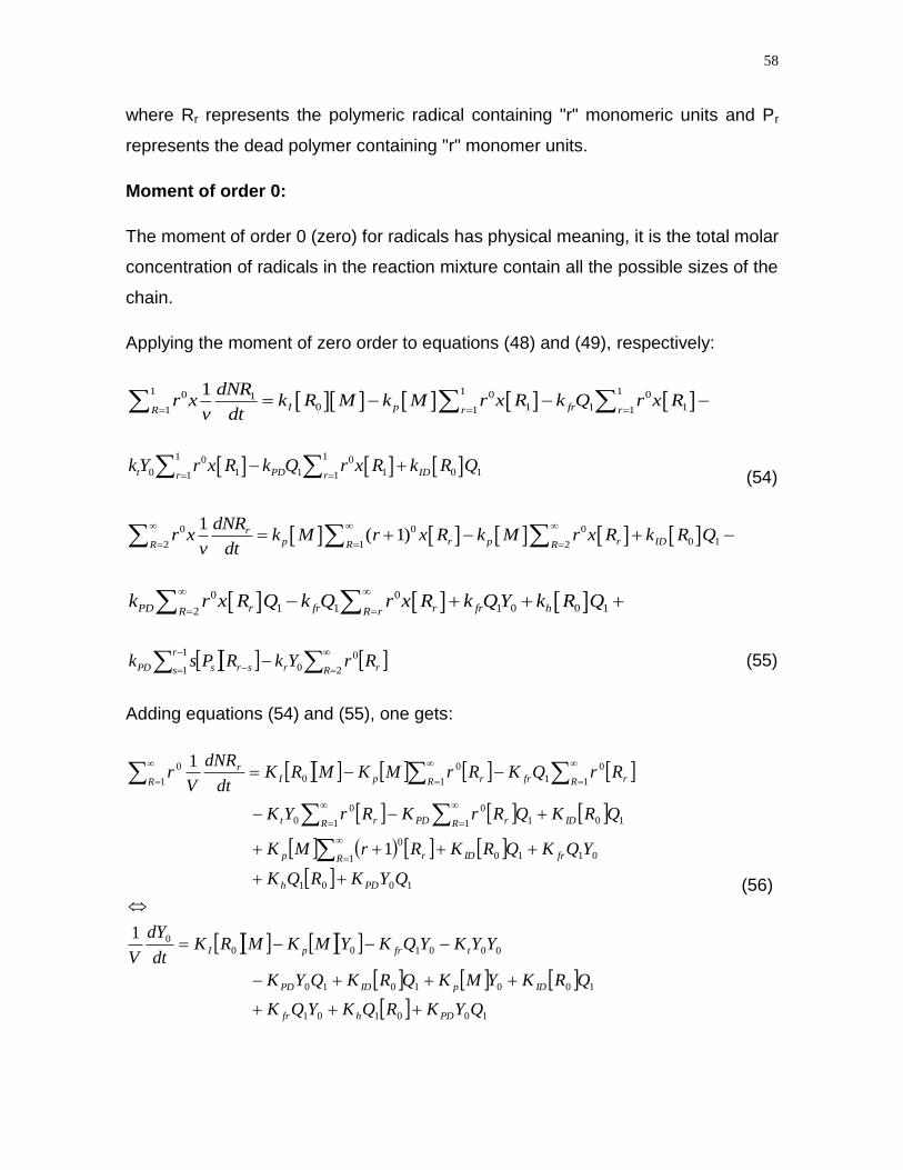
58

where Rr represents the polymeric radical containing "r" monomeric units and Pr

represents the dead polymer containing "r" monomer units.

Moment of order 0:

The moment of order 0 (zero) for radicals has physical meaning, it is the total molar

concentration of radicals in the reaction mixture contain all the possible sizes of the

chain.

Applying the moment of zero order to equations (48) and (49), respectively:

1 1 10 0 01

0 1 1 11 1 1

1I p frR r r

dNRr x k R M k M r x R k Q r x R

v dt

1 10 0

0 1 1 1 0 11 1t PD IDr rk Y r x R k Q r x R k R Q

(54)

0 0 0

0 12 1 2

1( 1)r

p r p r IDR R R

dNRr x k M r x R k M r x R k R Q

v dt

0 0

1 1 1 0 0 12PD r fr r fr hR R rk r x R Q k Q r x R k QY k R Q

rRr

r

s srsPD RrYkRPsk

2

0

0

1

1 (55)

Adding equations (54) and (55), one gets:

100101

1001010

000100

0

1001

01101

0

1011

0

1

0

0

1

0

11

0

01

0

1

1

1

QYKRQKYQK

QRKYMKQRKQYK

YYKYQKYMKMRKdt

dY

V

QYKRQK

YQKQRKRrMK

QRKQRrKRrYK

RrQKRrMKMRKdt

dNR

Vr

PDhfr

IDpIDPD

tfrpI

PDh

frIDrRp

IDrRPDrRt

rRfrrRpIr

R

(56)

59

Thus simplifying the above equation, we arrive at the following expression:

2

0011000 2

1YKRQKQRKMRK

dt

dY

VthIDI (57)

Applying the hypothesis pseudo- steady state (PSSH), we obtain:

2

0 0 1 1 0 02 0I ID h tk R M k R Q k Q R k Y (58)

This is an equation of second order to be solved using the Bhaskara formula

(Souza, 2013).

Moment of first order

For the development of the balance equations of the moment of first order, the

same reasoning used in the equations of moment of order 0 applies, differing only

in the multiplication factor, which goes from r0 to r1. The final expression is deduced

below:

10 0 0 2 1 1 1 1 2 0 2 0I p ID PD fr h fr

dYk R M k Y M k R Q k QY k QY k Q R k Q Y

dt

2 0 1 1 0 1PD tk Q Y QY k Y Y

1011020202

1101200011

YYkYQYQkYQkRQk

YQkYQkQRkMYkMRkdt

dY

V

tPDfrh

frPDIDpI

(59)

Applying the case of the pseudo-steady state is obtained:

0 0 0 2 2 0 2 0 2 0

1

1 0

I p ID h fr PD

fr t

k R M k Y M k R Q k Q R k Q Y k Q YY

k Q k Y

(60)

Overall moment for the dead Polymer

Following the reasoning used to refer to the moments of the polymeric radicals, the

following equations are obtained:

60

Moment of zero order:

2

0

2

00110100

2

1YkY

kRQkQYkQRk

dt

dQ

Vtd

tchPDID (61)

Moment of first order

101002112020201 2

2

1YYkYY

kRQkQYkQYkQYkQRk

dt

dQ

Vtd

tchfrfrPDID (62)

Given this, it is necessary to eliminate the Q2 equation model. To this end, it

replaces Y1 expression of the moment of order 1, and isolating Q2:

MYkMRkdt

dQ

VPI 00

11 (63)

3.4.3 Numerical Fractionation Technique

For polymerization systems that form gels (polymer network), the moments

of order higher than 1 diverges (i.e., tends to infinite) at the gel point (the point at

which the gel is formed). The technique of numerical fractionation was developed

by Teymour and Campbell (1994) to deal with these problems. In this technique,

the overall polymer population is divided numerically into a series of sub-

distributions, called "generations", having similar scale or degree of clustering and

sizes, due to the process through which they were formed. As one moves from one

generation to the next, the average molecular size will grow geometrically, thus

leading (at least theoretically) toward a generation of infinitely large polymer

molecules, which is the gel. At the beginning of the process, there are only linear

chains, grouped as "Generation Zero". Then the first crosslinks are formed, e.g.,

when a primary radical reacts with a pendant double bond (PDB) of a linear chain,

forming a branched chain ("First Generation") (Figure 7). Polymer chains of the

First Generation can continue reacting with linear chains, still remaining in the First

Generation. The change to the "Second Generation" occurs when two chains of

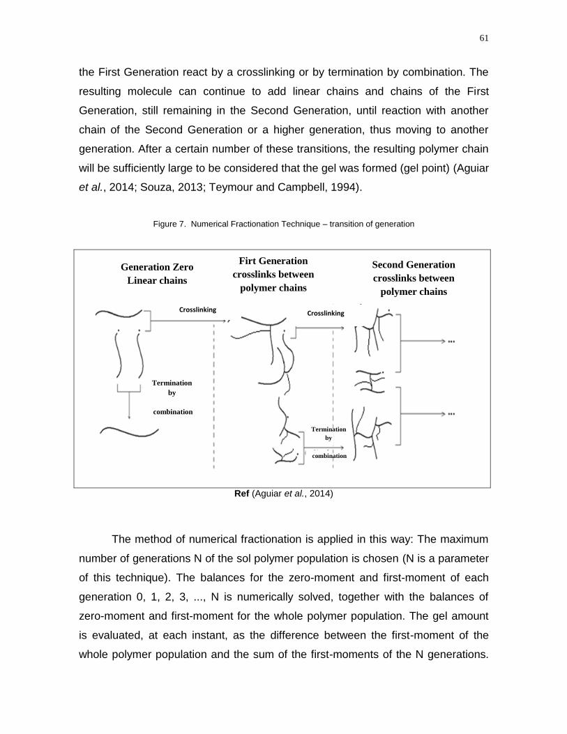
61

the First Generation react by a crosslinking or by termination by combination. The

resulting molecule can continue to add linear chains and chains of the First

Generation, still remaining in the Second Generation, until reaction with another

chain of the Second Generation or a higher generation, thus moving to another

generation. After a certain number of these transitions, the resulting polymer chain

will be sufficiently large to be considered that the gel was formed (gel point) (Aguiar

et al., 2014; Souza, 2013; Teymour and Campbell, 1994).

Figure 7. Numerical Fractionation Technique – transition of generation

Ref (Aguiar et al., 2014)

The method of numerical fractionation is applied in this way: The maximum

number of generations N of the sol polymer population is chosen (N is a parameter

of this technique). The balances for the zero-moment and first-moment of each

generation 0, 1, 2, 3, ..., N is numerically solved, together with the balances of

zero-moment and first-moment for the whole polymer population. The gel amount

is evaluated, at each instant, as the difference between the first-moment of the

whole polymer population and the sum of the first-moments of the N generations.

Termination

by

combination

Crosslinking

Termination

by

combination

Generation Zero

Linear chains

Firt Generation

crosslinks between

polymer chains

Crosslinking

Second Generation

crosslinks between

polymer chains

62

The simulation is repeated for different number of generations N until the result

does not change significantly and become independent of N. Teymour and

Campbell (1994) states that the use of 5 generations is usually enough to achieve

this condition.

Balance equations for the zero generation

The generation zero contains only linear chains.

Polymeric radicals of zero generation

011

000

YkQkQk

MRkY

tPDfr

I

(64)

0 00

01

1 1 0

I p

fr PD t

k R M k Y MY

k Q k Q k Y

(65)

011

00010

02

2

YkQkQk

YYMkMRkY

tPDfr

pI

(66)

Dead Polymer of the zero generation

Zero Order

000

2

0000100100101001000

2)(

YYk

Yk

RQkYQYQkQYkQRkdt

dQ

td

tchfrPDID

(67)

First Order:

001

000100201100202002001 )(

YYk

YYkRQkYQYQkQYkQRkdt

dQ

td

tchfrPDID

(68)

63

Second Order:

002

2

010002

00302103003003002

YYkYYYk

RQkYQkQYkQYkQRkdt

dQ

tdtc

hfrfrPDID

(69)

Balance equations for first generation

Polymeric radicals of first generation

Zero Order

01011

110001101001101011010

10YkQkQQk

QQRkQQYkQQRkQQYkY

tfrPD

IDPDhfr

(70)

First Order

01011

01110012100201010002

12002012002012002010

11YkQkQQk

YQYQYQYQYQk

QRQRkQRQRkQYQYkMYk

YtfrPD

PD

IDhfrp

(71)

Second Order

01011

02110112001311021003020101020003

1303013030130301011

12

222

2

YkQkQQk

YQYQYQYQYQYQYQYQk

QQRkQQRkQQYkMYMYk

YtfrPD

PD

IDhfrp

(72)

Death Polymer of first generation

Zero Order

100 11 0 11 11 0 1 10 11 0 00 11 0 10( )ID PD fr h tc td

dQk R Q k Y Q k Q Y QY k Q R k Y Y k Y Y

dt

(73)

Firts Order

110 12 0 12 12 0 1 11 12 0 11 00 10 01 11 0( )ID PD fr h tc tc td

dQk R Q k Y Q k Q Y QY k Q R k Y Y k Y Y k Y Y

dt

(74)

64

Second Order

012120011011002

01312101313013012

)2( YYKYYYYYYK

RQKYQKYQKQYKQRKdt

dQ

tdtc

hfrfrPDID

(75)

Balance equations for the generation "i"

Polymeric radicals of generation “i”

Zero Order

01

1

0 1,1

1,0

1

0 0,1,0,11,11,01,0

0

YkQkQQk

QRkYQYQkQRkQYkY

tfr

i

j jPD

iID

i

j jiiiPDihifr

i

(76)

First Order

01

1

0 1,1

1

0 1,1,

1

0 0,2,

1

0 2,0,1,11,10,12,1

2,02,02,00,

1

YkQkQQk

YQYQQYYQYQk

QRkQRkQYkMYk

Y

tfr

i

j jPD

i

j ji

i

j ji

i

j jiiiiiPD

iIDihifrip

i

(77)

Second Order

01

1

0 1,1

1

0 1,2,

1

0 0,3,

1

0 2,1,

2,11,1

1

0 3,0,1,12,10,13,1

3,03,03,00,1,

2

2

22

22

2

YkQkQQk

YQYQQY

YQQYYQYQk

QRkQRkQYkYYMk

Y

tfr

i

j jPD

i

j ji

i

j ji

i

j ji

ii

i

j jiiiii

PD

iIDihifriip

i

(78)

Death Polymer of generation “i”

Zero Order

00

1

00

2

0,1

01010110100

2itd

i

j joi

i

tc

ihiifriPDiIDi

YYkYYY

k

RQkYQYQkQYKQRkdt

dQ

(79)

65

2

2 2 13

1 0

2 i i ii

i i

Q Q QQ

Q Q

First Order

01

1

0 01

1

0 101.10.1

02110220201

YYkYYYYYYk

RQkYQYQkQYkQRkdt

dQ

itd

i

j ji

i

j jiiitc

ihiifriPDiIDi

(80)

Second Order

1

0 0

1

0 211

1

0 20

2

0,12,10.1

2003210330302

2i

j j

i

j iji

i

j jiiiitc

itdihiifriPDiIDi

YYYYYYYYYk

YYkRQkYQYQkQYkQRkdt

dQ

(81)

Application of closure relation of Saidel and Katz (1968);[Aguiar., 2014]; [Souza,

2013]:

66

CHAPTER IV

EXPERIMENTAL SECTION

In this chapter, the materials and equipments used are described and the

experimental procedures are explained.

4.1 Materials

Acrylic acid (AA) (Sigma-Aldrich, 99% purity, containing 200 ppm of MEHQ

as inhibitor) was used as the main water-soluble monomer. Trimethylolpropane

triacrylate (TMPTA) (Sigma Aldrich, containing 600 ppm of MEHQ)) and

tetraallyloxyethane (TAO) were used as crosslinkers (multifunctional monomers).

Sodium persulfate (Sigma-Aldrich) was employed as initiator. Toluene (Quimica

Moderna) was chosen as the inert continuous phase in the inverse-suspension

polymerizations, and Span 60 (Sigma Aldrich) as stabilizer. Hydroquinone (Sigma-

Aldrich) was used as inhibitor to shortstop the polymerization reaction in the

samples taken from the reactor. Unless otherwise stated, the reagents were used

as received, without further purification.

Tables 3 and 4 present the formulation of the hydrogels prepared by the

homopolymerization and by the copolymerization process, for the different studies.

The effects of five experimental variables were investigated: temperature, initiator

concentration, feed rate, crosslinker agent concentration and monomer

concentration.

In Runs E1 to E14 (Table 3), monomer conversion was measured as a

function of time. In Runs E5, E10 and E14, in addition to the monomer conversion,

the gel fraction was also measured along the experiments.

In all experiments in Table 3, the reaction medium was continuously

sparged with nitrogen to deoxygenate the mixture during the whole duration of the

run, in order to reduce the effect of the inhibition by the dissolved oxygen in water.

67

Table 3. Experimental Conditions

Formulation

Run T

(°C)

Toluene

(g)

Span

60

(g)

Water

(g)

Acrylic

Acid

(g)

TMPTA

(g)

EGDMA

(g)

TAO

(g)

Sodium

Persulfate

(g)

Feeding

Time

(min)

E1 70 191.18 3.54 30.8870 7.8443 0.1016 0 0 0.1512 40

E2 60 191.25 3.88 35.2797 7.7132 0.1081 0 0 0.15 40

E3 50 192.8 3.58 29.7509 7.714 0.1208 0 0 0.1522 40

E4 60 192.85 3.51 30.7055 7.713 0 0 0.1 0.1598 40

E5 60 196.12 3.56 34.5494 7.717 0 0 0.057 0.1569 40

E6 60 191.8 3.68 29.9852 7.68 0.1015 0 0 0.0689 40

E7 60 190.85 3.6 30.4854 7.8196 0.117 0 0 0.07581 40

E8 60 190.72 3.8 31.1329 7.8759 0.1175 0 0 0.1546 60

E9 60 190.99 3.61 26.3136 3.5363 0.10 0 0 0.1546 40

E10 60 191.75 3.6 30.2885 7.7702 0.05 0 0 0.1199 40

E11 60 193.47 3.59 30.0425 7.844 0.14 0 0 0.11 40

E12 60 191.4 4.0 30.1472 7.7218 0 0 0 0.2088 40

E13 60 646.5 12.09 141.76 26.2791 0 0 0 0.869 40

E14 60 193.78 3.72 30.4835 7.7866 0 0.0633 0 0.1976 40

Experiments E15 to E18 in Table 4 were carried out under conditions similar

to E6, except that the time of bubbling nitrogen in the reaction medium was varied

to assess the possible inhibition effect of the dissolved oxygen. In these

experiments, the monomer was previously purified by removing the inhibitor, as will

be explained below.

68

Table 4. Experimental conditions for the runs of the study of Inhibition period.

Inhibition Period

Run T

°C

Toluene

(g)

Span

60

(g)

Water

(g)

Acrylic

Acid

(g)

TMPTA

(g)

Induction

Period

(min)

Sodium

Persulfate

(g)

Feeding

Time

(min)

E15 60 191.8 3.68 29.9852 7.68 0.1015 0 0.0689 40

E16 60 191.8 3.68 29.9852 7.68 0.1015 15 0.0689 40

E17 60 191.8 3.68 29.9852 7.68 0.1015 30 0.0689 40

E18 60 191.8 3.68 29.9852 7.68 0.1015 60 0.0689 40

4.2 Equipments

The inverse suspension polymerizations were carried out in a a 250 mL five-

necked jacketed glass reactor, equipped with an impeller, reflux condenser, a

dropping tube (buret), a thermometer, and nitrogen line. The reactor is shown in

Figure 8. Water from a thermostatic bath circulated through the reactor jacket to

control the temperature and discharge valve.

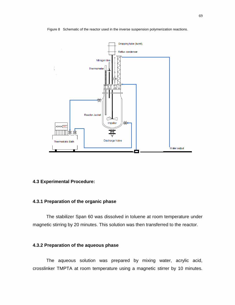
69

Figure 8 Schematic of the reactor used in the inverse suspension polymerization reactions.

4.3 Experimental Procedure:

4.3.1 Preparation of the organic phase

The stabilizer Span 60 was dissolved in toluene at room temperature under

magnetic stirring by 20 minutes. This solution was then transferred to the reactor.

4.3.2 Preparation of the aqueous phase

The aqueous solution was prepared by mixing water, acrylic acid,

crosslinker TMPTA at room temperature using a magnetic stirrer by 10 minutes.

70

Then the initiator (sodium persulfate) dissolved in a small amount of water was

added to this mixture at room temperature.

4.3.3 Polymerization runs

The prepared organic solution (Span 60 and toluene) was transferred a 250

mL four-necked jacketed glass reactor. Water from a thermostatic bath flows

through the jacket to control the temperature. The reactor content was heated

(under a mild stream of nitrogen bubbling to remove dissolved oxygen from the

medium) until reached the desired temperature.

Then the aqueous solution, composed of acrylic acid, crosslinker (when

used), sodium persulfate and water, transferred to the buret, was added dropwise

to the organic phase under an agitation speed of 400 rpm. The duration of the

feeding was 40-60 min. At the end of the aqueous phase feeding period, the first

sample was withdrawn from the reactor and the time was set to zero.

After finishing the feeding of the aqueous solution, samples were taken at

different times along the operation time for the analysis of monomer conversion

and gel content.

4.3.4 Purification monomer

Commercial monomers have some amount of inhibitor MEHQ to prevent

spontaneous polymerization in the storage flask. Inhibitors and retarders are

characterized by having the ability to form a stabilized free radical. The standard

inhibitor level in commercial acrylic acid (Sigma-Aldrich) is 200 ppm Monomethyl

Ether of Hydroquinone (MEHQ), and in commercial TMPTA (Sigma-Aldrich) is 600

ppm.

Experiments E6 and E15-E18 were performed with monomer (and

crosslinker) without inhibitor MEHQ (Mono Methyl Ether of Hydroquinone).

71

Monomers can be purified in lab scale by steam or vacuum distillation. In the

present study, vacuum distillation was used (Figure 9). During the distillation, a

copper gauze was placed in the monomer to inhibit polymerization.

Following the safety recommendations, after distillation, acrylic acid and

TMPTA should be stored at a temperature range of 18 to 25 °C, to prevent any

crystallization (freezing point = 13 °C). It is recommended that the monomers be

stored indoors at a temperature lower than 25°C and away from light, under air

atmosphere (because oxygen acts also as an inhibitor).

Figure 9. Vacuum Distillation equipment used for removing the MEHQ inhibitor.

4.3.5 Study of the inhibition period

The inhibition period, usually observed in polymerization of commercial

monomers, is the initial period of process in which no formation of polymer (no

consumption of monomer) takes place from the starting of the polymerization

Copper Gauze

72

process. This occurs due to the presence of inhibitor. Besides to inhibitor present

in commercial grade monomers, oxygen is also a very active inhibitor for most free

radical polymerization processes. Moreover, the solubility of oxygen in water is

sufficiently high.

In order to study the effect of the oxygen as an inhibitor, the procedure

proposed by Cutié et al. (1996) and Li et al. (2006) was employed in the present

work. After removed the commercial MEHQ inhibitor from the monomer, it was

aerated with air for 60 min to allow the saturation of the solution with oxygen. Then,

the solution was deoxygenated at different levels by bubbling with nitrogen for 15,

30, and 60 min (as indicated in Table 4). Monomer deoxygenated at different levels

was employed in the polymerization runs (E15-E18) to test the effect of different

oxygen concentrations on the monomer conversion. These runs were conducted

with low concentration of initiator (0.03% wt) in order to maximize the effect under

study.

4.3.6 Gravimetric analysis for conversion

The monomer conversion during the polymerization was determined by

gravimetric analysis, using analytical balance (with accuracy of 0.0001 g). An

empty glass container (Beaker) is previously weighed (m1) and then an amount (~

0.25 mL) of aqueous solution of 2 %wt hydroquinone (inhibitor) was added (to

shortstop the reaction), and the flask is weighed (m2). Then, a sample of ~10 mL

taken from the reactor is poured into the flask and weighed again (m3). Samples

were kept immersed in an ice bath, Figure 10, to prevent further polymerization. At

the end of the experimental run, all samples were placed in an oven at 68°C for 48

hours in order to remove the volatile components (toluene and unreacted

monomer). Then the samples were weighed again several times over a period of 4

days to ensure that the dry sample reached a constant weight (m4). Figure 11

illustrates the wet and dry samples.

73

Figure 10. Samples immersed in an ice bath Figure 11. Dry samples

The conversion was calculated by equation (83):

idacryliccac

ehydoquinonspan

fmm

fmmfmmmmX

)(

)()()(

23

12602314

(83)

where

m1 = weight of the empty Beaker flask (g),

m2 = weight of the flask with hydroquinone solution (g)

m3 = weight of the flask with the sample taken from the reactor plus HQ (g),

m4 = weight of the flask with the dry sample (g),

fhydroquinone = weight fraction of the hydroquinone solution added to the sample

fspan60 = weight fraction of Span 60 in the formulation,

facrylic acid = weight fraction of acrylic acid in the formulation.

74

4.3.7 Determination of gel fraction by Soxhlet system

The gel fraction of polymer samples was determined by extracting the sol

fraction (soluble fraction) using a Soxhlet-type equipment (Soxtherm Gerhardt

Multistat/SX PC), composed of 6 extraction units, multistate control unit, extraction

glass beakers, filter paper, compressed air supply and thermal bath equipment,

shown in Figure 12 (http://soxtherm.gerhardt.de/en/).

Figure 12. Soxhlet extraction equipment

A sample of dry polymer was placed inside the thick filter paper (previously

weighed, m5) and weighed (m6). The filter paper with the polymer sample was

placed in the extraction thimble, which was then loaded into the main chamber of

the Soxtherm extractor. The extraction solvent (water, in the present case) was

placed in the distillation flask and heated to reflux for 3 hours for the extraction of

the soluble fraction of polymer (sol fraction). The filter paper with the insoluble

polymer was then dried in an oven for about 24 hours, left in a desiccator for 2

hours for cooling down to the ambient temperature and then weighed (m7).

75

The following equation was used to determinate the gel fraction:

)(

)(

56

57

mm

mmGF

(84)

where

m5 = weight of the empty filter paper (g),

m6 = weight of the initial dry polymer sample and the filter paper (g),

m7 = weight of the final dry sample after extraction and filter paper (g).

76

CHAPTER V

RESULTS AND DISCUSSIONS

In this Chapter, the experimental results of monomer conversion and gel

fraction measured in the different experiments are presented and discussed. The

results are also compared with the prediction of the mathematical model, and the

sensitivity of the certain key parameters is tested.

The runs were performed typically, as a base case, in a total of four hours in

batch operation, after 40 min of feeding period before the time zero (time was set

to zero at the end of the feeding period), at temperature of 60°C and stirring speed

of 400 rpm. Runs with changes in these conditions were carried out to assess the

effects of the process conditions on the process performance.

5.1 Conversion measured by Gravimetry

5.1.2 Homopolymerization

Figure 13 presents the evolution of the monomer conversion measured

during the homopolymerization of acrylic acid in run E12, in which no

multifunctional monomer (crosslinker) was used.

The monomer conversion increased very slowly during the first 40 minutes

(probably an effect of retardation/inhibition), and then increased fast, reaching

conversion of almost 80% at 160 min. The last two points, measured at

conversions above 60%, seems to be higher than the trend, probably an indication

of autoacceleration effect (gel effect).

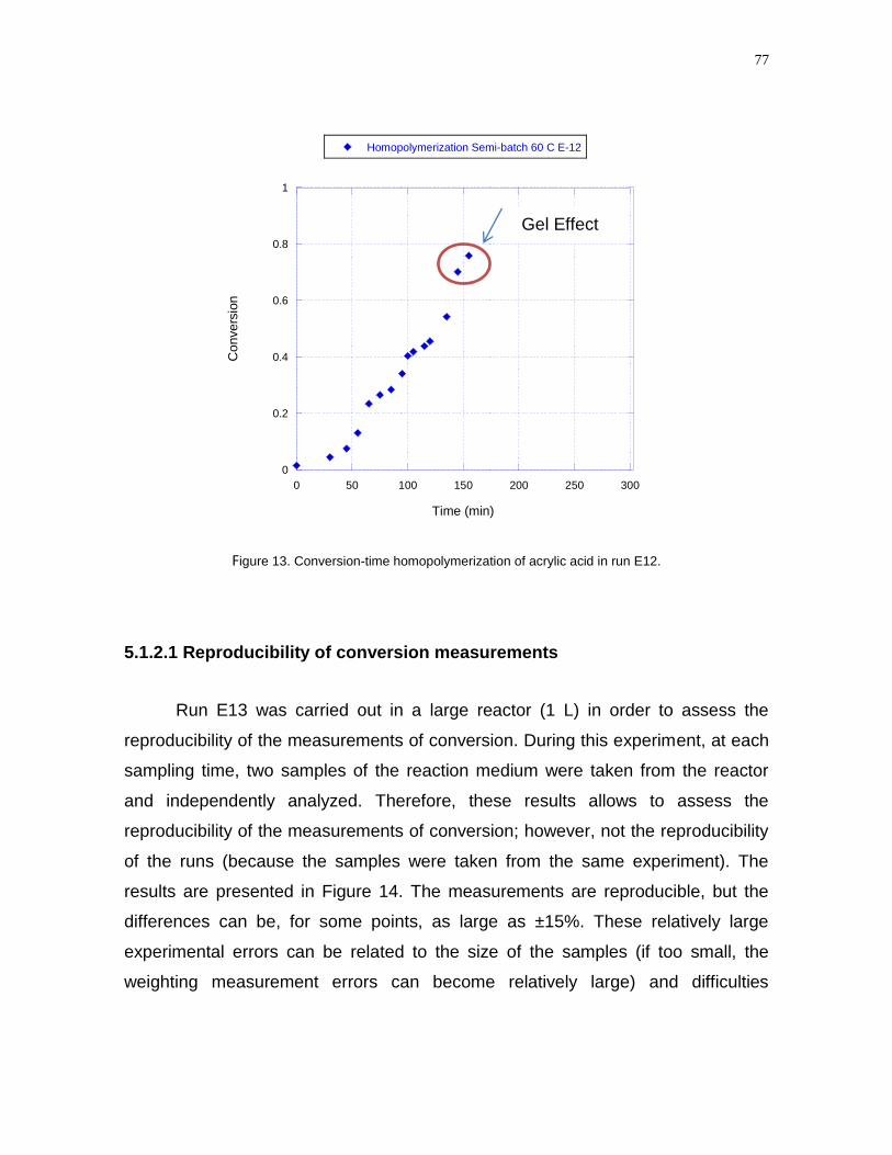
77

0

0.2

0.4

0.6

0.8

1

0 50 100 150 200 250 300

Homopolymerization Semi-batch 60 C E-12

Co

nvers

ion

Time (min)

Figure 13. Conversion-time homopolymerization of acrylic acid in run E12.

5.1.2.1 Reproducibility of conversion measurements

Run E13 was carried out in a large reactor (1 L) in order to assess the

reproducibility of the measurements of conversion. During this experiment, at each

sampling time, two samples of the reaction medium were taken from the reactor

and independently analyzed. Therefore, these results allows to assess the

reproducibility of the measurements of conversion; however, not the reproducibility

of the runs (because the samples were taken from the same experiment). The

results are presented in Figure 14. The measurements are reproducible, but the

differences can be, for some points, as large as ±15%. These relatively large

experimental errors can be related to the size of the samples (if too small, the

weighting measurement errors can become relatively large) and difficulties

Gel Effect

78

involved in complete drying of the sample due to formation of dry skin on the film

surface.

Figure 14. Conversion-time homopolymerization of acrylic acid during run E13 and run E13 replicated.

5.1.3 Copolymerization

In this section, experimental data of conversion for the different

copolymerization runs are presented and discussed. The effects of different

process variables, such as, temperature, crosslinker type, crosslinker

concentration, acrylic acid concentration, initiator concentration, duration of feeding

period, etc., are analyzed by comparing the results of runs performed under similar

conditions, having, when possible, only significant variation of the variable under

analysis (one variable at a time).

Experiments T (°C)

Toluene (g)

Span 60 (g)

Water (g)

Acrylic Acid (g)

TMPTA (g)

EGDMA (g)

TAO (g)

Sodium Persulfate

(g)

Feeding Time (min)

E13 60 646.5 12.09 141.76 26.2791 0 0 0 0.869 40

79

5.1.3.1 Effect of temperature

Experiments E1, E2 and E3 were carried out at different temperatures, 70,

60 and 50°C, respectively. The conversion-versus-time variations for these runs

are presented in Figure 15.

It is evident from this figure that the duration of the induction period changes

with the temperature. However, the rate of polymerization (after the end of the

induction period) seems to be almost the same for the three runs.

Run T (°C)

Toluene (g)

Span 60 (g)

Water (g)

Acrylic Acid (g)

TMPTA (g)

EGDMA

(g) TAO (g)

Sodium Persulfate

(g)

Feeding Time (min)

E1 70 191.18 3.54 30.8870 7.8443 0.1016 0 0 0.1512 40

E2 60 191.25 3.88 35.2797 7.7132 0.1081 0 0 0.15 40

E3 50 192.8 3.58 29.7509 7.714 0.1208 0 0 0.1522 40

0

0.2

0.4

0.6

0.8

1

0 50 100 150 200 250 300

Temp 50 °C- Copolymerization E-3Temp 60 °C Copolymerization E-2Temp 70 °C Copolymerization E-1

Co

nvers

ion

Time(min)

Figure 15. Conversion-time inverse suspension polymerization at different temperatures

For run E3 at 50 °C, the conversion was low (~10-15%) for the first 180 min,

then increased, but reached a relatively low final conversion, stopped at ~72%.

Run E1 at 70°C presented a much shorter induction period (~70 min) and then

80

increased the polymerization rate, reaching complete conversion (100%) at 145

minutes. These observations are in accord to the classical theory of free radical

polymerization: at higher temperature, the decomposition of the initiator is faster,

thus generating more radicals and consuming faster the initial amount of inhibitor,

thus reducing the induction period.

Curiously, however, the complete final conversion (100%) was obtained in

even short period for run E2, which was performed at the intermediate

temperature, 60°C. Run E2 apparently had no strong induction period, as the initial

conversion at time zero (i.e., at the time immediately after the feeding period) was

surprisingly high (~25%).

5.1.3.2 Effect of Crosslinker Type

The effect of the crosslinker type was studied by performing experiments

with similar conditions changing the type of crosskinking agent. The results for run

E14 (with bi-functional crosslinker EGDMA), run E10 (with tri-functional crosslinker

TMPTA) and run E5 (with tetra-functional crosslinker TAO) are presented in Figure

16 and 17.

In this Figure, the highest polymerization rate was observed for EGDMA and

the lowest for TAO, the conversion-versus-time curve for TMPTA presenting an

intermediate behavior. The direct interpretation of these results is difficult due to

the differences in functionality and molar mass, as these runs were performed with

about the same weight concentration of the crosslinkers. Moreover, the reactivity of

the different crosslinkers with acrylic acid can be different, as well as the reactivity

of the different pendant double bonds left by each of the crosslinkers.

Run T (°C)

Toluene (g)

Span 60 (g)

Water (g)

Acrylic Acid (g)

TMPTA (g)

EGDMA (g)

TAO (g)

Sodium Persulfate

(g)

Feeding Time (min)

E5 60 196.12 3.56 34.5494 7.717 0 0 0.057 0.1569 40

E10 60 191.75 3.6 30.2885 7.7702 0.05 0 0 0.1199 40

E14 60 193.78 3.72 30.4835 7.7866 0 0.0633 0 0.1976 40

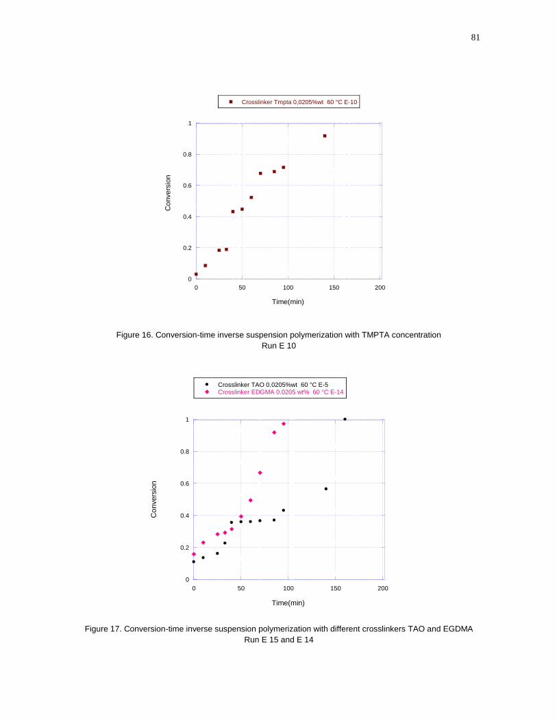
81

0

0.2

0.4

0.6

0.8

1

0 50 100 150 200

Crosslinker Tmpta 0,0205%wt 60 °C E-10

Co

nvers

ion

Time(min)

Figure 16. Conversion-time inverse suspension polymerization with TMPTA concentration

Run E 10

0

0.2

0.4

0.6

0.8

1

0 50 100 150 200

Crosslinker TAO 0.0205%wt 60 °C E-5Crosslinker EDGMA 0.0205 wt% 60 °C E-14

Co

nvers

ion

Time(min)

Figure 17. Conversion-time inverse suspension polymerization with different crosslinkers TAO and EGDMA

Run E 15 and E 14

82

5.1.3.3 Effect of initiator concentration

Figure 18 shows the effect of the initiator (sodium persulfate) concentration

on the polymerization rate. The overall rate of polymerization increased with

initiator concentration, as expected from the classical theory of free-radical

polymerization, which predicts the rate of polymerization to be proportional to the

square-root of the initiator concentration. The average polymerization rate for run

E6 was ~0.60 %/min, while was ~0.85 %/min for run E2.

Also, the delay (induction period), caused by the presence of commercial

inhibitor MEHQ in the monomer, was a little longer for the run with lower initiator

concentration, which is also in accord with the classical theory of free-radical

polymerization.

Run T (°C)

Toluene (g)

Span 60 (g)

Water (g)

Acrylic Acid (g)

TMPTA (g)

EGDMA

(g) TAO (g)

Sodium Persulfate

(g)

Feeding Time (min)

E2 60 191.25 3.88 35.2797 7.7132 0.1081 0 0 0.1500 40

E6 60 191.80 3.68 29.9852 7.6800 0.1015 0 0 0.0689 40

0

0.2

0.4

0.6

0.8

1

0 50 100 150 200 250 300

Initiator Concentration NPS 0.06%wt-60 °C E-2Initiator Concentration NPS 0.03%wt-60°C E-6

Co

nvers

ion

Time (min)

Figure 18. Conversion-time inverse suspension polymerization at different Sodium Persulfate concentration

Run E 2 and E 6

83

5.1.3.4 Effect of the Feeding Time

The effect of the duration of the feeding of aqueous solution (containing

acrylic acid, TMPTA, sodium persulfate and water) to the reactor, before the zero-

time of the batch process, was analyzed in Figure 20, in which the conversion-

versus-time curves for runs E2 (feeding time 40 min) and E8 (feeding time 60 min)

are compared.

Run T (°C)

Toluene (g)

Span 60 (g)

Water (g)

Acrylic Acid (g)

TMPTA (g)

EGDMA

(g) TAO (g)

Sodium Persulfate

(g)

Feeding Time (min)

E2 60 191.25 3.88 35.2797 7.7132 0.1081 0 0 0.1500 40

E8 60 190.72 3.80 31.1329 7.8759 0.1175 0 0 0.1546 60

0

0.2

0.4

0.6

0.8

1

0 50 100 150 200 250 300

Copolymerization Feed Flow Rate 40min 60°C E-2 Copolymerization Feed Flow Rate 60min 60°C E-8

Co

nvers

ion

Time(min)

Figure 19. Conversion-time inverse suspension polymerization at different feed flow rate time

Run E 2 and E 8

For run E8 (longer feeding time, 60 min), no induction time is observed, but

the polymerization during the batch period was slower (0.3 %/min), see Figure 20.

For run E2 (shorter feeding time, 40 min) Figure 21, an induction time of about 50-

60 min was observed, followed by a period of faster polymerization (1.0 %/min).

84

0

0.05

0.1

0.15

0.2

0.25

0.3

0.35

0 0.2 0.4 0.6 0.8 1

Polymerization rate % min

Po

lym

erization r

ate

% m

in

Conversion

Figure 20. Conversion-Polymerization rate of inverse suspension polymerization Run E8

0.075

0.08

0.085

0.09

0.095

0.1

0.105

0.11

0.2 0.3 0.4 0.5 0.6 0.7 0.8 0.9

Polymerization Rate % min E2

Po

lym

erization R

ate

% m

in

Conversion

Figure 21. Conversion-Polymerization rate of inverse suspension polymerization Run E2

85

5.1.3.5 Effect of acrylic acid concentration

Experiments E2 and E9 were carried out under similar conditions except the

concentration of acrylic acid, which was ~3.20wt% in E2 and ~1.20wt% in E9. The

results of these two runs are compared in Figure 22.

Run T (°C)

Toluene (g)

Span 60 (g)

Water (g)

Acrylic Acid (g)

TMPTA (g)

EGDMA

(g) TAO (g)

Sodium Persulfate

(g)

Feeding Time (min)

E2 60 191.25 3.88 35.2797 7.7132 0.1081 0 0 0.1500 40

E9 60 190.99 3.61 26.3136 3.5363 0.1000 0 0 0.1546 40

0

0.2

0.4

0.6

0.8

1

0 50 100 150 200 250 300

Acrylic Acid concentration 3.20% E-2Acrylic Acid concentration 1.20% wt E-9

Co

nvers

ion

Time (min)

Figure 22. Conversion-time inverse suspension different acrylic acid concentration

Run E2 and E9

The induction time was about 140 min for run E9 and about 30 min for run

E2. This result indicates that the induction time is caused not only by the inhibitor

86

MEHQ that comes with the commercial monomers. If MEHQ was the only inhibitor

responsible for the induction time, the expected effect is directly proportional to the

presence of oxygen and impurities. However, the opposite behavior is observed in

Figure 22. Therefore, this effect is probably ascribed to the presence of oxygen as

an additional inhibitor. It should be mentioned that the control of the nitrogen

feeding was not very precise, so variations of the nitrogen flow between the

different runs may be the cause for the differences in induction time observed.

After the end of the induction period, the polymerization occurred fast in both

runs E9 and E2. The polymerization rate was 1.53 %/min for run E9 and 2.5 %/min

for run E2. Comparing these values with the monomer concentration in the two

runs, the apparent order for monomer was 1.6, which is in accordance to the value

1.5 reported in the literature for solution polymerization of acrylic acid (Cutié et al.,

1997b; Qui et al., 2016; Lorber et al., 2010) and 1.7 for precipitation polymerization

of acrylic acid (Bunyakan et al., 1999).

5.1.3.6 Effect of Deoxygenation

Experiments E15, E16, E17 and E18 were carried out to evaluate the effect

of the deoxygenation period (after saturation of the initial solution with air). These

experiments are similar to those performed by Cutié et al. (1997a). The aqueous

solution, prepared with purified, distilled monomers (without MEHQ), was aerated

by 60 minutes, then the solution was bubbled with nitrogen during different periods

of time to partially deoxygenate the solution and then used in the polymerization

experiments. The objective was to analyze the inhibition effect of dissolved oxygen.

The results are presented in Figures 23-26, and compared with experiment

E6, performed under similar conditions but with commercial monomer (containing

inhibitor MEHQ).

Figure 23 compares run E6 and run E15 (for which no deoxygenation was

done). For the remaining experiments, the duration of deoxygenation time was

increased progressively (15 min for E-16, 30 min for E17, 60 min for E18) and the

87

results are presented in Figures 23-26. The ultimate rates of polymerization show

little dependence on the deoxygenation conditions, but the magnitude of the

induction time depends strongly on the deoxygenation conditions.

The presence of oxygen did not diminish (significantly) the rate of reaction,

but rather lengthened the induction period, indicated that oxygen was an inhibitor

rather than a retarder for this polymerization. However, slow inlet of air into the

reactor (due to incomplete sealing and insufficient bubbling of inert gas) would

result in a polymerization that appears retarded.

Run T °C

Toluene (g)

Span 60 (g)

Water (g)

Acrylic Acid (g)

TMPTA (g)

Deoxygenation Period (min)

Sodium Persulfate

(g)

Feeding Time (min)

E6 60 191.8 3.68 29.9852 7.68 0.1015 --- 0.0689 40

E15 60 191.8 3.68 29.9852 7.68 0.1015 0 0.0689 40

E16 60 191.8 3.68 29.9852 7.68 0.1015 15 0.0689 40

E17 60 191.8 3.68 29.9852 7.68 0.1015 30 0.0689 40

E18 60 191.8 3.68 29.9852 7.68 0.1015 60 0.0689 40

0

0.2

0.4

0.6

0.8

1

24 44 64 104 124

E-6No Deox- E 15

Co

nvers

ion

Time (min)

Figure 23. Polymerization rate and inhibition time as a function of deoxygenation conditions. No deoxygenation

88

0

0.2

0.4

0.6

0.8

1

24 44 64 104 124

E-615 min Deox E 16

Co

nvers

ion

Time (min)

Figure 24. Polymerization rate and inhibition time as a function of deoxygenation conditions. 15 min deoxygenation

0

0.2

0.4

0.6

0.8

1

24 44 64 104 124

E-630 min Deox E 17

Co

nvers

ion

Time (min)

Figure 25. Polymerization rate and inhibition time as a function of deoxygenation conditions. 30 min deoxygenation

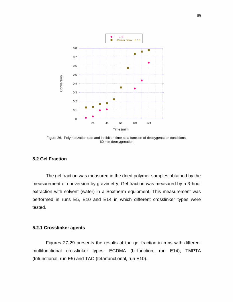
89

0

0.1

0.2

0.3

0.4

0.5

0.6

0.7

0.8

24 44 64 104 124

E-660 min Deox E 18

Co

nvers

ion

Time (min)

Figure 26. Polymerization rate and inhibition time as a function of deoxygenation conditions. 60 min deoxygenation

5.2 Gel Fraction

The gel fraction was measured in the dried polymer samples obtained by the

measurement of conversion by gravimetry. Gel fraction was measured by a 3-hour

extraction with solvent (water) in a Soxtherm equipment. This measurement was

performed in runs E5, E10 and E14 in which different crosslinker types were

tested.

5.2.1 Crosslinker agents

Figures 27-29 presents the results of the gel fraction in runs with different

multifunctional crosslinker types, EGDMA (bi-function, run E14), TMPTA

(trifunctional, run E5) and TAO (tetarfunctional, run E10).

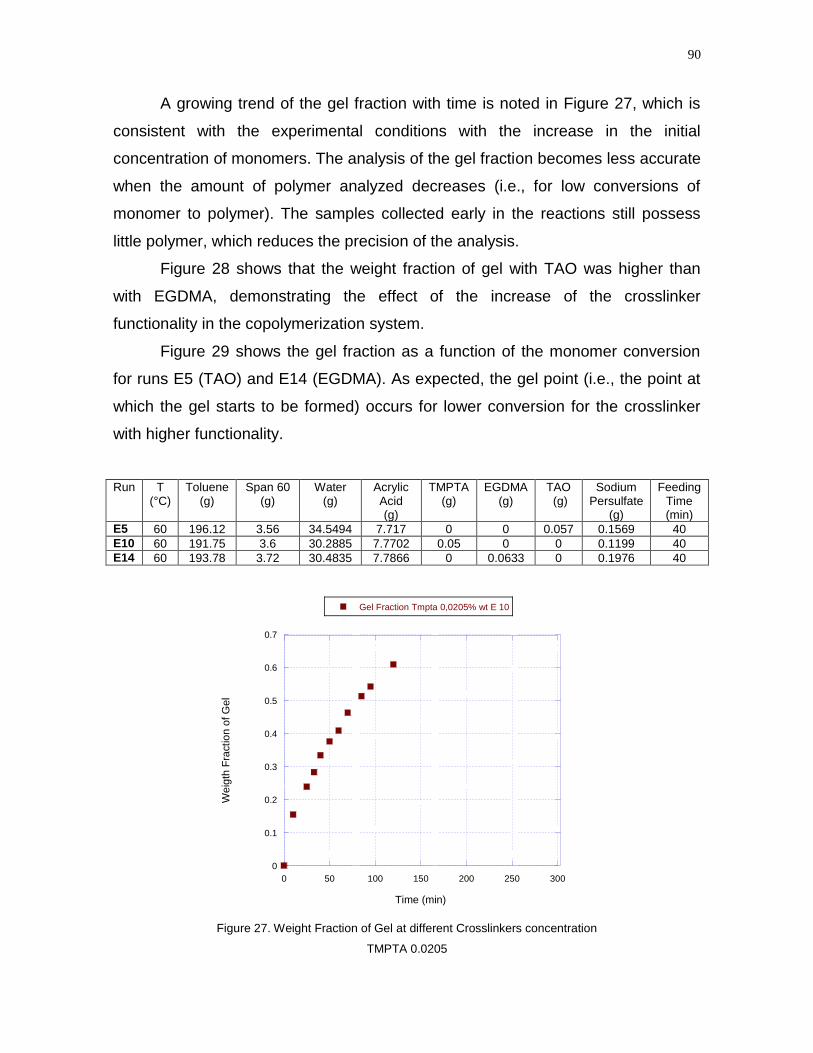
90

A growing trend of the gel fraction with time is noted in Figure 27, which is

consistent with the experimental conditions with the increase in the initial

concentration of monomers. The analysis of the gel fraction becomes less accurate

when the amount of polymer analyzed decreases (i.e., for low conversions of

monomer to polymer). The samples collected early in the reactions still possess

little polymer, which reduces the precision of the analysis.

Figure 28 shows that the weight fraction of gel with TAO was higher than

with EGDMA, demonstrating the effect of the increase of the crosslinker

functionality in the copolymerization system.

Figure 29 shows the gel fraction as a function of the monomer conversion

for runs E5 (TAO) and E14 (EGDMA). As expected, the gel point (i.e., the point at

which the gel starts to be formed) occurs for lower conversion for the crosslinker

with higher functionality.

Run T (°C)

Toluene (g)

Span 60 (g)

Water (g)

Acrylic Acid (g)

TMPTA (g)

EGDMA (g)

TAO (g)

Sodium Persulfate

(g)

Feeding Time (min)

E5 60 196.12 3.56 34.5494 7.717 0 0 0.057 0.1569 40

E10 60 191.75 3.6 30.2885 7.7702 0.05 0 0 0.1199 40

E14 60 193.78 3.72 30.4835 7.7866 0 0.0633 0 0.1976 40

0

0.1

0.2

0.3

0.4

0.5

0.6

0.7

0 50 100 150 200 250 300

Gel Fraction Tmpta 0,0205% wt E 10

We

igth

Fra

ctio

n o

f G

el

Time (min)

Figure 27. Weight Fraction of Gel at different Crosslinkers concentration

TMPTA 0.0205

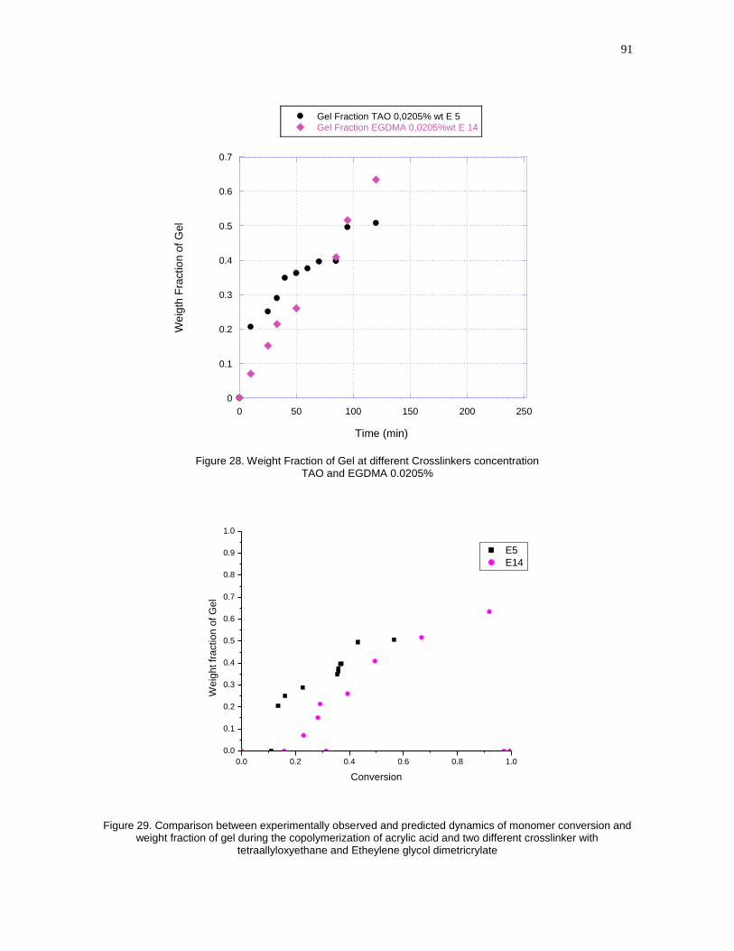
91

0

0.1

0.2

0.3

0.4

0.5

0.6

0.7

0 50 100 150 200 250

Gel Fraction TAO 0,0205% wt E 5Gel Fraction EGDMA 0,0205%wt E 14

We

igth

Fra

ctio

n o

f G

el

Time (min)

Figure 28. Weight Fraction of Gel at different Crosslinkers concentration TAO and EGDMA 0.0205%

0.0 0.2 0.4 0.6 0.8 1.0

0.0

0.1

0.2

0.3

0.4

0.5

0.6

0.7

0.8

0.9

1.0

We

igh

t fr

actio

n o

f G

el

Conversion

E5

E14

Figure 29. Comparison between experimentally observed and predicted dynamics of monomer conversion and weight fraction of gel during the copolymerization of acrylic acid and two different crosslinker with

tetraallyloxyethane and Etheylene glycol dimetricrylate

92

5.3. Simulation results and comparison with experimental data

In this section, the results of the model simulation are compared with the

experimental data.

Table 5 shows the values of the kinetic parameters used in the model

developed in the present work.

Table 5. Kinetic parameters used in the preliminary analysis of the mathematical model developed

*Variable changing propagation rate constant

As presented in Chapter 3, the model was developed on the basis of the

recent study by Gonçalves et al. (2011) to simulated the synthesis of acrylic acid

hydrogels using a kinetic model based on the population balance equations and

generating functions in order to predict the changes in the properties like the gel

fraction and monomer conversion.

Reaction Kinetic Parameters Unit

Initiator Decomposition (Sodium persulfate)

10 226001,433 10

1,987dk Exp

T

f =0,7

s

-1

Initiation 1 1 5Ij p jk k j

L.mol-1

s-1

Chain Transfer for polymer 0frk

L.mol-1

s-1

Hydrogen Abstration 0hk

L.mol-1

s-1

Termination by combination 75 10tck

L.mol-1

s-1

Termination by disproportionation 0tdk

L.mol-1

s-1

*Propagation rate constant Kp11

11

1 11

var ,

1 5

p

pi p

k iavel

being

k k i

L.mol-1

s-1

*Crosslinker Reactivity ratios

r31 = kp13/kp11

r43 = kp43/kp13

r31 =0.3 r43 =0.1 r31 =2.31 r43 =0.25

93

5.3.1 Effect of the value of the propagation rate constant (kp11)

Gonçalves et al. (2011) reported some values of propagation kinetic

constant (Tables 7 and 8), and its dependency of temperature and monomer

concentration.

Table 6. Reported values of the termination rate constant (kp11) of acrylic acid in water

Ref: (Gonçalves et al., 2011)

For generality, no particular chemical system has been selected for this

study, but the chosen kinetic parameters should allow a simulation as much as

possible close to the real behavior of the crosslinking copolymerization systems. A

basic set of kinetic parameters were fixed in the calculations in order to have a

realistic time evolution of the copolymerization; they are collected in the

supplementary material.

The comparison of the monomer conversion profile (AA) between the model

and the experimental data is presented in Figures 30 to 43, showing the effect of

the variation of the propagation rate constant (kp11).

94

Table 7. Reported values of the propagation rate constant (kp11) of acrylic acid in water

Ref: (Gonçalves et al., 2011)

95

0 50 100 150 200 250 3000

0.1

0.2

0.3

0.4

0.5

0.6

0.7

0.8

0.9

1

Time(min)

Co

nve

rsio

n

E 12

Kp11-1200L/mol.s

5.3.2 Simulation of Homopolymerization

Figure 30 shows the comparison of the simulation results with the

experimental data of monomer conversión for the homopolymerization of acrylic

acid during run E12. Because the effect of inhibitor was not explicitly accounted for

in the model, in the simulation, an induction time of 30 minutes, based on the

experimental data, was assumed. In order to make the simulation results closer to

the experimental data, the parameter KP11, the propagation rate constant for acrylic

acid, was adjusted to a value equal to 1200 L/(mol.s). This value allowed fitting

reasonably the trend of the experimental data, except for the last two points that

indicated an autoacceleration effect (“gel effect”, or diffusion-controlled

termination).

The procedure for model adjusting was simply by repeated simulations and

trial-and-error. The model could be further improved by refining the search of the

parameter value by a formal optimization routine and by include the

autoacceleration effect (diffusion-controlled termination), but this was not employed

in the present work.

Figure 30.Conversion-time Homopolymerization process at 60°C

96

5.3.3 Copolymerization Simulation

5.3.3.1 Reaction Temperature

Figure 31 to 33 shows the comparison between model results and

experimental data for the runs E1, E2 and E3 carried out at different temperatures

(50 to 70 °C). The procedure included, again, the shifting of the simulated curves

by an induction time obtained directly from the experimental data. In run E2 (70 °C,

Figure 31), the induction time was assumed to be 75 minutes and the fitted value

of KP11 was 6000 L/(mol.s). For run E2 (60 °C, Figure 32), no induction time was

needed and the fitted value of KP11 was 5000 L/(mol.s). For run E3 (50 °C, Figure

33) the induction time assumed was 180 minutes and the adjusted value of KP11

was 4500 L/(mol.s).

0 50 100 150 200 250 3000

0.1

0.2

0.3

0.4

0.5

0.6

0.7

0.8

0.9

1

Time(min)

Co

nve

rsio

n

E 1

Kp11-6000 L/mol.s

Figure 31.Conversion-time dependence of the rate coefficient for the homopropagation of acrylic acid Kp11

70°C

97

0 50 100 150 200 250 300 3500

0.1

0.2

0.3

0.4

0.5

0.6

0.7

0.8

0.9

1

Time (min)

Con

ve

rsio

n

E 2

Kp11-5000 L/mol.sktc= 5e7 L/mol.sr21=1.2987

Figure 32. Conversion-time dependence rate coefficient for the homopropagation of acrylic acid Kp11 60°C

0 50 100 150 200 250 3000

0.1

0.2

0.3

0.4

0.5

0.6

0.7

0.8

0.9

1

Time (min)

Co

nve

rsio

n

E3

Kp 11-4500 L/mol.s

Figure 33. Conversion-Time different values of the rate coefficient for the homopropagation of acrylic acid Kp11

50°C

No clear explanation can be drawn from the values of the induction time,

which is known to depend on the presence of inhibitors MEHQ (which comes in the

commercial monomers used) and oxygen (which can be dissolved in the aqueous

solution). Although nitrogen was bubbled in all experiments to deoxygenate the

reaction medium, the nitrogen flow rate was not precisely controlled nor was equal

98

in all experiments. This is probably the reason for the differences in induction time

observed experimentally.

On the other hand, the values of KP11, manipulated to fit the experimental

trend, showed the expected tendency of increase progressively with the increasing

in temperature.

5.3.3.2 Crosslinkers

Figures 34 to 36 show the adjusted model curves for runs E5 (crosslinker

TAO), E10 (crosslinker TMPTA) and E14 (crosslinker EGDMA). In these runs, no

strong induction time was observed and then the induction time was assumed to

be zero in the simulations. The values of adjusted KP11 were in the range 1500-

3000 L/(mol.s). Although the adjust was reasonable, no clear trend was observed

between the values of KP11 and the functionality of the crosslinker (1500 L/(mol.s)

for TAO, 3000 L/(mol.s) for TMPTA and 2000 L/(mol.s) for EGDMA), reflecting the

experimental tendency of the experimental conversion-versus-time curves.

0 50 100 150 200 250 3000

0.1

0.2

0.3

0.4

0.5

0.6

0.7

0.8

0.9

1

Time (min)

Con

ve

rsio

n

E 5

Kp11-1500 L/mol.s

Figure 34. Conversion-time different values of rate coefficient homopropagation of acrylic acid (Kp11) influence of crosslinkers TAO

99

0 50 100 150 200 250 300 3500

0.1

0.2

0.3

0.4

0.5

0.6

0.7

0.8

0.9

1

Time (min)

Con

ve

rsio

n

E 10

Kp11-3000 L/mol.sKtc= 5e7 L/mol.sr21=1.2987

Figure 35. Conversion-time dependence of the rate coefficient homopropagation of acrylic acid (Kp11) influence of crosslinkers TMPTA 60 °C

0 50 100 150 200 250 3000

0.1

0.2

0.3

0.4

0.5

0.6

0.7

0.8

0.9

1

Time (min)

Co

nve

rsio

n

E 14

Kp11-2000 L/mol.s

Figure 36. Conversion-time rate different values of the coefficient homopropagation of acrylic acid (Kp11) Influence of crosslinkers EGDMA

100

5.3.3.3 Run with low concentration of Sodium persulfate

Figure 37 compares the experimental results and simulation of run E-6, in

which a lower concentration of sodium persulfate (0.03wt %) was employed. Based

on the experimental data, the induction time used in the simulation was assumed

to be 30 minutes. The adjusted value of KP11 was 1700 L/(mol.s).

0 50 100 150 200 250 3000

0.1

0.2

0.3

0.4

0.5

0.6

0.7

0.8

0.9

1

Time (min)

Co

nve

rsio

n

E 6

Kp11-1700L/mol.s

Figure 37. Conversion-time different values of the rate coefficient for the homopropagation of acrylic acid

(Kp11 ) influence low initiator concentration of sodium persulfate

5.3.3.4 Run with long feeding time of the aqueous phase

Figure 38 compares the experimental and simulated results for Run E8 that

was performed after a longer feeding time (60 minutes, before the time zero). No

induction time was considered in the simulation and a value of KP11 = 1000

L/(mol.s) was adjusted.

The purpose of this experiment was to analyze if there occurs kinetic

changes in relation to feeding from the aqueous phase and how it could affect the

reaction medium.

101

0 50 100 150 200 250 3000

0.1

0.2

0.3

0.4

0.5

0.6

0.7

0.8

0.9

1

Time (min)

Co

nve

rsio

n

E 8

Kp11-1000 L/mol.s

Figure 38. Conversion-time different values of the rate coefficient homopropagation of acrylic acid (Kp11)–

influence on feed flow rate time

5.3.2.5 Run with low concentration of acrylic acid

The experiment E9 was conducted at low initial concentration of monomer.

Figure 38 shows the experimental and simulation results. An unexpectedly long

induction time was observed (a value of 154 minutes was assumed to fit the model

to this run) and a the adjusted value of KP11 was 3000 L/(mol.s).

0 50 100 150 200 250 3000

0.1

0.2

0.3

0.4

0.5

0.6

0.7

0.8

0.9

1

Time (min)

Con

ve

rsio

n

E 9

Kp 11- 3000 L/mol.s

Figure 39. Conversion-time different values of the rate coefficient for the homopropagation of acrylic acid

(Kp11 ) different acrylic acid concentration at 60°C

102

5.3.3.6 Deoxygenation period

Experiments E15, E16, E17 and E18, all conducted with a low concentration

of initiator, are shown in Figures 40 to 43. The commercial monomer containing

200 ppm of MEHQ was previously purified by distillation, aerated by bubbling air

for 60 minutes, and then deoxygenated by bubbling nitrogen for different

deoxigenation times (0, 15, 30 and 60 minutes).

0 50 100 150 200 250 3000

0.1

0.2

0.3

0.4

0.5

0.6

0.7

0.8

0.9

1

Time (min)

Co

nve

rsio

n

E 15

Kp 11-1500 L/mol.s

Figure 40. Conversion-time dependence rate coefficient homopropagation of acrylic acid (Kp11), 1500 L/mol.s -Polymerization rate and inhibition time as a function of deoxygenation condition- No Deox

0 50 100 150 200 250 3000

0.1

0.2

0.3

0.4

0.5

0.6

0.7

0.8

0.9

1

Time (min)

Co

nve

rsio

n

E 16

Kp11-5000 L/mol.s

Figure 41. Conversion-time dependence of rate coefficient homopropagation of acrylic acid (Kp11) 5000 L/mol.s -Polymerization rate and inhibition time as a function of 15 min of deoxygenation condition

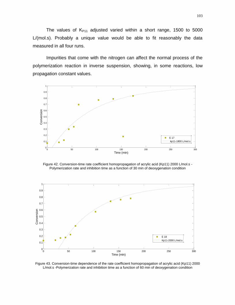
103

The values of KP11 adjusted varied within a short range, 1500 to 5000

L/(mol.s). Probably a unique value would be able to fit reasonably the data

measured in all four runs.

Impurities that come with the nitrogen can affect the normal process of the

polymerization reaction in inverse suspension, showing, in some reactions, low

propagation constant values.

0 50 100 150 200 250 3000

0.1

0.2

0.3

0.4

0.5

0.6

0.7

0.8

0.9

1

Time (min)

Co

nve

rsio

n

E 17

kp11-1800 L/mol.s

Figure 42. Conversion-time rate coefficient homopropagation of acrylic acid (Kp11) 2000 L/mol.s -Polymerization rate and inhibition time as a function of 30 min of deoxygenation condition

0 50 100 150 200 250 3000

0.1

0.2

0.3

0.4

0.5

0.6

0.7

0.8

0.9

1

Time (min)

Co

nve

rsio

n

E 18

Kp11-2000 L/mol.s

Figure 43. Conversion-time dependence of the rate coefficient homopropagation of acrylic acid (Kp11) 2000 L/mol.s -Polymerization rate and inhibition time as a function of 60 min of deoxygenation condition

104

5.4 Analysis of the dynamics of gelation by the numerical fractionation

technique

In this section, a comparison is presented between the gel fraction profile

obtained from the model developed in this work.

The reactivity ratios for pendant double bond polymerization was

evaluated in these simulations, as shown from Figures 44 to 46 , to observe its

effect on the model curves of gel fraction.

Also, the effect of the number of generations considered in the simulations

was also studies. The number of generations is a parameter of the numerical

fractionation technique by Teymour (1994). In principle, the higher the number of

generations considered, the better the approximation of the model to calculate the

gel fraction. On the other hand, the increase of number of generations causes an

increase in the computational effort to solve the model. Therefore, the number of

generations should be chosen as the lowest value to which the further increase

does not change significantly the model responses.

In the simulations, it was observed that the computer program does not

provide good results when more than 5 generations is chosen. This limitation is

probably related to the use of an ODE solver for nonstiff systems (ode45) in the

MATLAB program. When the number of generations was increased, the stiffness of

the ODE system increased and the solver failed.

The effect of the number of generations on the simulation results is shown in

Figure 44. It can be seen that the differences in the simulated value of gel fraction

decrease as the number of generations increases. The difference becomes

negligible for simulations with 4 and 5 generations, indicating the use of 5

generations is sufficient to the correct prediction of the gel fraction.

105

0 50 100 150 200 250 3000

0.05

0.1

0.15

0.2

0.25

0.3

0.35

0.4

0.45

0.5

Time (min)

We

igh

t F

ractio

n o

f G

el

Generation number=1

Generation number=2

Generation number=3

Generation number=4

Generation number=5

Figure 44. Evolution of the gel fraction calculated using different numbers of generations (n = 1, 2 3, 4 and 5).

The effect of the reactivity of the PDBs on the dynamics of gel formation is

shown in Figures 45 and 46. These simulations were performed with 5

generations. Under these conditions, the reactivity of pendant double bonds (rPDB)

has an effect on the dynamics of gel formation. As expected, lower gel content is

predicted if the reactivity of PDBs is much lower than for the double bonds of the

crosslinker (rPDB 0.3). The gel content increases with the increase of the value of

this parameter (rPDB), as shown in Figure 46 (in comparision with Figure 45). Due

to the low content of crosslinker in the polymerization system, the overall monomer

conversion (not shown) is almost insensitive to this parameter. The reactivity of the

all the three double bonds of TMPTA to react with acrylic acid would be expected

to, but once incorporated into the polymer network, the reactivity of the other two

remaining double bonds are assumed to be lower.

106

0 50 100 150 200 250 3000

0.1

0.2

0.3

0.4

0.5

0.6

0.7

Time (min)

We

igth

Fra

ctio

n o

f G

el

rpdb31=0.3rpdb43=0.1Generation number=5

Figure 45. Evolution of the gel fraction calculated with numerical fractionation technique with 5 generations

using different reactivity ratios of PDBs

0 50 100 150 200 250 3000

0.1

0.2

0.3

0.4

0.5

0.6

0.7

0.8

0.9

Time (min)

We

igth

Fra

ctio

n o

f G

el

rpdb 31=2.31rpdb 43=0.25Gonçalves (2011)Generation Number=5

Figure 46. Evolution of the gel fraction calculated with numerical fractionation technique with 5 generations

using different reactivity ratios of PDBs

107

5.5 General discussions

This work was proposed to evaluate some key variables of the process of

inverse suspensions polymerization of acrylic acid (and crosslinkers) to produce

hydrogel. Experiments were carried out in laboratory-scale reactor and monomer

conversion and gel fraction were measured as a function of time during the

polymerization. The effects of initiator concentration, feed flow rate, crosslinker

concentration and monomer concentration on these results were evaluated.

These possible scenarios may account for some sources of different

induction period, uncertainties at different stages of the experimentation and the

analytical testing methods used for calculation of polymerization rate and inhibition

time, as function of deoxygenation conditions, which need to be considered. The

induction period varied a lot in the different runs, reflecting either the presence of

MEHQ inhibitor in the commercial monomers (different concentrations due to

different lots of monomer, or different storage time of the same lot) or the effect of

the dissolved oxygen in the aqueous phase. A limited number of experiments were

performed with purified acrylic acid monomer (which was distilled to remove the

inhibitor) trying to assess the effect of dissolved oxygen by changing the

deoxygenation time.

Three types of crosslinkers, namely trimetylolpropane triacrylate (TMPTA),

tetraallyloxyethane (TAO) and ethylene glycol dimethacrylate (EGDMA), were

employed in the experiments to compare their effectiveness as a comonomer/

crosslinker. This kind of crosslinking agent is typically used for generating highly-

crosslinked polymer structures, thus increasing polymer toughness, modulus and

solvent resistance. An increase in the comonomer functionality dramatically

decreases the general mobility of monomer functional group in the medium during

polymerization due to the earlier formation of a crosslinked network hydrogel even

at very low conversions. For example, trimethylol propane triacrylate, a trifunctional

monomer, is less sensitive to oxygen inhibition than the bifunctional comonomer.

Monomer structure may also be a significant factor in reducing oxygen inhibition

especially when monomers have abstractable hydrogen such as vinyl ether

groups, which are among the most common functional groups.

108

The conversion profiles over all conditions and modes of operation are

generally well represented by a model that uses, after the adjustment of the

propagation rate constant for acrylic acid (Kp11) and imposing in the simulations an

initial period of induction caused by the inhibition. This induction time was obtained

from the experimental observation. The quantitative prediction of the effect of the

inhibitor on the simulated results would require to change the kinetic model in order

to include explicitly the inhibition reactions, which is easy to do, but would require

the estimation of the involved kinetic parameters of the inhibition process. This

would require additional measurements in experiments specially designed for this

purpose.

109

CHAPTER VI

CONCLUSIONS AND SUGGESTIONS

6.1 Conclusions

In this topic the main conclusions and contributions are presented:

In the present work, experimental studies and mathematical model were

developed for the homopolymerization and copolymerization of acrylic acid in an

inverse suspension polymerization process, for the determination of the monomer

conversion and gel fraction. The effects of temperature, monomer concentration,

concentration and type of of the comonomer/crosslinker, concentration of the

initiator, and feeding time of the aqueous phase were studied.

The results contribute to increase the database of experimental data of this

process and to test the mathematical model, thus contribute to improve the general

knowledge on this complex process.

The experimental measurements of monomer conversion by gravimetry

presented errors of about 15%. This is still acceptable, but is higher than the usual

uncertainties of this method. These errors are related to the size of the samples

and to the formation of dry skin in the samples during drying. This reinforces the

special care required in conversion measurements in gelling polymerization

systems.

For some runs, gel fraction was measured by extraction with solvent (water),

which is also a delicate measurement technique subject to errors related to the

incomplete extraction and with the propagation of the weighting errors due to very

small samples involved. The obtained results for gel fraction were sound and

acceptable, indicating the employed extraction method was reliable.

Some polymerization reactions showed extensive induction time, which was

caused by the presence of dissolved oxygen and the content of MEHQ inhibitor in

110

the commercial-grade monomer. Some experiments were performed with distilled

monomer and by changing the dissolved oxygen in a systematic way, yet the

dissolved oxygen was not directly measured. These results show that both oxygen

and MEHQ affect the results.

A mathematical model for the process was developed based on the previous

models reported in the literature, in special that of Gonçalves et al. (2011). The

model predicted the time history of monomer conversion and gel fraction to be

compared with the data collected in the experiments.

The model does not account for explicitly the inhibition reactions, so it is not

capable of predict the induction time observed experimentally. In order to account

for the induction period in the simulated curves, the zero time of the simulated

curves were shifted towards higher times by adding a specified value of induction

time directly estimated from the experimental data.

After this induction time, the simulated curves were fitted to the experimental

data by adjusting the value of the kinetic constants of propagation of acrylic acid

(KP11), in a similar way performed in the literature (Arriola et al., 1996; Gonçalves

et al., 2011). The obtained values of this rate constant increases with temperature,

as expected.

The gel fraction was calculated in the model by using the numerical

fractionation technique. The number of generations was studied and determined

that 5 generations were sufficient for the gel fraction calculation.

The comparison of gel fraction predictions with the experimental data shows

that additional fitting should be necessary, because the model is predicting that the

gel point occurs much after the gel point started in practice.

In summary, this research provided new experimental data and a better

understanding of some of the variables affecting the inverse suspension

polymerization of acrylic acid and TMPTA. The mathematical model developed for

this process is suitable to represent the main features of this system, was partially

111

adjusted to the monomer conversion data and should be better fitted to the gel

fraction by adjusting additional kinetic parameters.

6.2 Suggestions for Future Work

The following suggestions can be recommended to future works in this topic:

Improve the mathematical model to account for the effect of inhibitors

The model could be improved by including explicitly the kinetics of the inhibition

by both dissolved oxygen and MEHQ. The work of Li and Schork (2006) would

provide a general basis to change the kinetic model and balance equations

accordingly. Specific experiments (see, e.g., Cutie et al., 1997) could be

designed to assess these effects and to allow for estimation of the unknown

parameters.

Study the kinetics with DSC and FTIR, and measurement of pH to

controlling to KP

Use of DSC is appropriate for recording the heat production of chemical and

physical process and for obtaining data changes with time to follow the kinetics

of the reaction. This allows determining the dependence of the polymerization

rate on various reaction parameters. And also use the FTIR in-line monitoring

technique, in order to determinate the monomer conversion and validate with

the gravimetric analysis, giving a better perspective of what is happening inside

the reactor

Study the hydrogel performance in controlled releasing of drugs

continuing the research to characterize the controlled release of pharmaceutical

products (like insulin) from the hydrogel matrix, performing and simulating

changes of pH, and identify which of the samples of hydrogels is the most

suitable for this process

112

Neutralization of Acrylic acid, aqueous solution of acrylic acid salts obtain

trough the neutralization of AA, with a base such as NaOH, are also usually

consider in SAP production, improving condition medium reaction due to pH

control , reach a higher conversion and also gel fraction results.

SEM micrographic of particles The particle size distributions of hydrogels, is

one of the topics of great importance in processes make by inverse suspension

polymerization and the dependence of absorption, studying the characteristics

on particle size using the MEV technique and determinate another variable

such as the salinity of the water on absorption effects, and develop a model to

accompany this type of research.

Swelling of crosslinkers is one of the important physical properties of

hydrogels and depend on the precise structure of the polymer network, of key

importance is equilibrium swelling capacity. The effect of different crosslinkers

(e.g., TMPTA, TAO and EGDMA) on the swelling capacity of the hydrogel.

Molecular theories of rubber elasticity describe with varying accuracy the

relationship between the molecular structure of a crosslinked polymer and the

amount of swelling. Crosslink density can be determined by the two methods,

modulus and swelling measurements.

NIR Infrared spectroscopy prediction of the evolution of monomer

concentration, conversion and average particle diameter in acrylic acid in

inverse suspension polymerization using different kind of initiators such as

AIBN, benzoyl peroxide, hydroperoxide. Multivariate partial least squares

calibration models can be developed to relate NIR spectra collected by the

immersion sensor with online conversion and polymer particle size data, values

predicted by the NIR calibration models and these latter were also able to

detect different types of operational disturbances.

113

REFERENCES

AGUIAR, L. G. et al. Development of Cyclic Propagation Kinetics for Modeling the

Nitroxide-mediated Radical Copolymerization of Styrene–Divinylbenzene

Macromolecular Reaction Engineering, v. 8, n. 4, p. 282–294, 2014.

AHMED, E. M. Hydrogel: Preparation, characterization, and applications. Journal

of Advanced Research, 2013.

ARRIOLA, D. J. et al. Crosslinker reactivity and the structure of superabsorbent

gels. Journal of Applied Polymer Science, v. 63, n. 4, p. 439–451, 1997.

BOWMAN, C. N.; PEPPAS, N. A. A kinetic gelation method for the simulation of

free-radical polymerizations. Chemical Engineering Science, v. 47, n. 6, p. 1411–

1419, 1992.

BUNYAKAN, C., & Hunkeler, D. Precipitation polymerization of acrylic acid in

toluene. I: synthesis, characterization and kinetics. Polymer, 40(23), 6213-6224.

(1999).

BUNYAKAN, C., & Hunkeler, D. Precipitation polymerization of acrylic acid in

toluene. II: synthesis, characterization and kinetics. Polymer, 40(23), 6213-6224.

(1999).

CHOUDHARY, M. S. Inverse Suspension Polymerization of Partially Neutralized

and Lightly Cross-Linked Acrylic Acid: Effect of Reaction Parameters.

Macromolecular Symposia, v. 277, n. 1, p. 171–176, 1 fev. 2009.

COSTA, M. R.; DIAS, R. Prediction of sol fraction and average molecular weights

after gelation for non-linear free radical polymerizations using a kinetic approach.

2003.

114

CUTIÉ, S. S. et al. The effects of MEHQ on the polymerization of acrylic acid in the

preparation of superabsorbent gels. Journal of Applied Polymer Science, v. 64, n.

3, p. 577–589, 18 abr. 1997.

CUTIÉ, S. S. et al. Acrylic acid polymerization kinetics. Journal of Polymer Science

Part B: Polymer Physics, v. 35, n. 13, p. 2029–2047, 30 set. 1997.

GONÇALVES, M. et al. Modeling studies on the synthesis of superabsorbent

hydrogels using population balance equations. 2011.

GUPTA, P.; VERMANI, K.; GARG, S. Hydrogels: from controlled release to pH-

responsive drug delivery. Drug Discovery Today, v. 7, n. 10, p. 569–579, 15 maio.

2002.

HARRISSON, S.; MACKENZIE, S. R.; HADDLETON, D. M. Pulsed Laser

Polymerization in an Ionic Liquid:  Strong Solvent Effects on Propagation and

Termination of Methyl Methacrylate. Macromolecules, v. 36, n. 14, p. 5072–5075, 1

jul. 2003.

HENNINK, W. E.; NOSTRUM, C. F. VAN. Novel crosslinking methods to design

hydrogels. Advanced Drug Delivery Reviews, v. 64, p. 223–236, dez. 2012.

HENTON, D. E.; POWELL, C.; REIM, R. E. The decomposition of sodium

persulfate in the presence of acrylic acid. Journal of Applied Polymer Science, v.

64, n. 3, p. 591–600, 1997.

H. OMIDIAN, M. J. Z.-M. Polymerization of sodium acrylate in inverse-suspension

stabilized by sorbitan fatty esters. European Polymer Journal, v. 39, n. 5, p. 1013–

1018, 2003.

115

HUSSAIN, Y. A.; LIU, T.; ROBERTS, G. W. Synthesis of Cross-Linked, Partially

Neutralized Poly(Acrylic Acid) by Suspension Polymerization in Supercritical

Carbon Dioxide. Industrial & Engineering Chemistry Research, v. 51, n. 35, p.

11401–11408, 5 set. 2012.

JAHANZAD, F.; SAJJADI, S.; BROOKS, B. W. Characteristic intervals in

suspension polymerisation reactors: An experimental and modelling study.

Chemical Engineering Science, v. 60, n. 20, p. 5574–5589, out. 2005a.

JAHANZAD, F.; SAJJADI, S.; BROOKS, B. W. Characteristic intervals in

suspension polymerisation reactors: An experimental and modelling study.

Chemical Engineering Science, v. 60, n. 20, p. 5574–5589, out. 2005b.

KALFAS, G.; YUAN, H.; RAY, W. H. Modeling and experimental studies of

aqueous suspension polymerization processes. 2. Experiments in batch reactors.

Industrial & Engineering Chemistry Research, v. 32, n. 9, p. 1831–1838, 1 set.

1993.

KIZILEL, S. et al. Mathematical Model for Vinyl-Divinyl Polymerization.

Macromolecular Reaction Engineering, v. 1, n. 6, p. 587–603, 20 nov. 2007.

KUCHTA, F.-D.; HERK, A. M. VAN; GERMAN, A. L. Propagation Kinetics of Acrylic

and Methacrylic Acid in Water and Organic Solvents Studied by Pulsed-Laser

Polymerization. Macromolecules, v. 33, n. 10, p. 3641–3649, 1 maio. 2000.

LACÍK, I.; BEUERMANN, S.; BUBACK, M. PLP−SEC Study into Free-Radical

Propagation Rate of Nonionized Acrylic Acid in Aqueous Solution.

Macromolecules, v. 36, n. 25, p. 9355–9363, 1 dez. 2003.

116

LIN, H.-R. Solution polymerization of acrylamide using potassium persulfate as an

initiator: kinetic studies, temperature and pH dependence. European Polymer

Journal, v. 37, n. 7, p. 1507–1510, jul. 2001.

LI, R.; SCHORK, F. J. Modeling of the Inhibition Mechanism of Acrylic Acid

Polymerization. Industrial & Engineering Chemistry Research, v. 45, n. 9, p. 3001–

3008, 1 abr. 2006.

LOISEAU, J. et al. Synthesis and Characterization of Poly(acrylic acid) Produced

by RAFT Polymerization. Application as a Very Efficient Dispersant of CaCO3,

Kaolin, and TiO2. Macromolecules, v. 36, n. 9, p. 3066–3077, 2003.

LORBER, N., Pavageau, B., & Mignard, E. Droplet-based millifluidics as a new

miniaturized tool to investigate polymerization reactions.Macromolecules, 43(13),

5524-5529. (2010).

MACHADO, F.; LIMA, E. L.; PINTO, J. C. A review on suspension polymerization

processes. Polímeros, v. 17, n. 2, p. 166–179, jun. 2007a.

MACHADO, F.; LIMA, E. L.; PINTO, J. C. Dynamic optimization of semibatch vinyl

acetate/acrylic acid suspension copolymerizations. Polymer Engineering &

Science, v. 50, n. 4, p. 697–708, 1 abr. 2010a.

MACHADO, F.; LIMA, E. L.; PINTO, J. C. Dynamic optimization of semibatch vinyl

acetate/acrylic acid suspension copolymerizations. Polymer Engineering &

Science, v. 50, n. 4, p. 697–708, 1 abr. 2010b.

MARCELO KAMINSKI LENZI, F. M. S. Semibatch styrene suspension

polymerization processes. Journal of Applied Polymer Science, v. 89, n. 11, p.

3021 – 3038, 2003.

117

MAYOUX, C. et al. Inverse suspension polymerization of sodium acrylate:

Synthesis and characterization. Journal of Applied Polymer Science, v. 77, n. 12,

p. 2621–2630, 19 set. 2000.

MURLI, C.; SONG, Y. Pressure-Induced Polymerization of Acrylic Acid: A Raman

Spectroscopic Study. The Journal of Physical Chemistry B, v. 114, n. 30, p. 9744–

9750, 2010.

NI, X. et al. Suspension polymerization of acrylamide in an oscillatory baffled

reactor: From drops to particles. AIChE Journal, v. 47, n. 8, p. 1746–1757, 1 ago.

2001.

OKAY, O. Gel growth in free radical crosslinking copolymerization: Effect of

inactive gel radicals. Macromolecular Theory and Simulations, v. 9, n. 6, p. 354–

361, 1 jul. 2000b.

OMIDIAN, H.; HASHEMI, S. A.; SAMMES, P. G.; MELDRUM, I. G. Modified

acrylic-based superabsorbent polymers. Effect of temperature and initiator

concentration. Polymer, v. 39, n. 15, p. 3459–3466, jul. 1998.

OMIDIAN, H. et al. Modified acrylic-based superabsorbent polymers (dependence

on particle size and salinity). Polymer, v. 40, n. 7, p. 1753–1761, mar. 1999.

PARK, H.; ROBINSON, J. R. Mechanisms of mucoadhesion of poly(acrylic acid)

hydrogels. Pharmaceutical Research, v. 4, n. 6, p. 457–464, dez. 1987.

QIU, L., Wang, K., Zhu, S., Lu, Y., & Luo, G. Kinetics study of acrylic acid

polymerization with a microreactor platform. Chemical Engineering Journal, 284,

233-239. (2006).

118

RINTOUL, I.; WANDREY, C. Polymerization of ionic monomers in polar solvents:

kinetics and mechanism of the free radical copolymerization of acrylamide/acrylic

acid. Polymer, v. 46, n. 13, p. 4525–4532, 17 jun. 2005.

SILVA, F. M.; LIMA, E. L.; PINTO, J. C. Control of the Copolymer Composition in

Suspension Copolymerization Reactions. Industrial & Engineering Chemistry

Research, v. 43, n. 23, p. 7312–7323, 1 nov. 2004.

SOUZA, E. F. Estudo experimental e modelação matemática do processo de

produção de hidrogéis de poli(ácido acrílico). 2013.

TEYMOUR, F.; CAMPBELL, J. D. Analysis of the Dynamics of Gelation in

Polymerization Reactors Using the “Numerical Fractionation” Technique.

Macromolecules, v. 27, n. 9, p. 2460–2469, 1994.

TOBITA, H.; HAMIELEC, A. E. Crosslinking kinetics in polyacrylamide networks.

Polymer, v. 31, n. 8, p. 1546–1552, 1 ago. 1990.

TOBITA, H.; HAMIELEC, A. E. Kinetics of free-radical copolymerization: the

pseudo-kinetic rate constant method. Polymer, v. 32, n. 14, p. 2641–2647, 1991.

TOBITA, H.; KUMAGAI, M.; AOYAGI, N. Microgel formation in emulsion

polymerization. Polymer, v. 41, n. 2, p. 481–487, jan. 2000.

VERROS, G. D.; ACHILIAS, D. S.; GIANNOUKOS, G. I. Development of a

comprehensive mathematical model for free radical suspension polymerization of

methyl methacrylate. Polymer Engineering & Science, v. 51, n. 4, p. 670–678, 1

abr. 2011.

WANG, G.; LI, M.; CHEN, X. Inverse suspension polymerization of sodium

acrylate. Journal of Applied Polymer Science, v. 65, n. 4, p. 789–794, 1997.

119

APPENDICE

APPENDICE A-. Chemical properties of reagents/Initial condition

Ref: https://en.wikipedia.org/.

Reagents

Chemical Properties

Molar Concentration

mol/L

Boling Temperature

°C

Melting Temperature

°C

Density g/ml

Sodium Persulfate 0.020207

- 180 2.59

Acrylic Acid 2.0 141 14 1.05 Trimetylolpropane Triacrylate 0.0004261

155 - 1.1

Tetraallytoxyethane 0.00015012

160 - 1.06

Ethylene glycol dimethacrylate

0.00017012

98 to 100 °C – 40 °C 1.051

120

APPENDICE B. Experimental runs-Matlab

Experiment Time (min) Conversion

E1 0 0.043249056 24 0.012490692 34 0.088700536 44 0.100011691 54 0.102162219 74 0.148058148 84 0.463276812 104 0.764417248 114 0.993500687

Experiment Time (min) Conversion

E2 0 0.251331285 24 0.26842 34 0.27823918 44 0.369273455 54 0.405575175 64 0.48117 84 0.880286592

Experiment Time (min) Conversion

E3 0 0.097795456 24 0.126431666 34 0.091220091 44 0.12666868 64 0.114684696 74 0.148845114 94 0.118550449 124 0.07202903 144 0.07182901 164 0.086728234 184 0.124342619 200 0.284232218 215 0.44624250 230 0.622375982 245 0.684803436

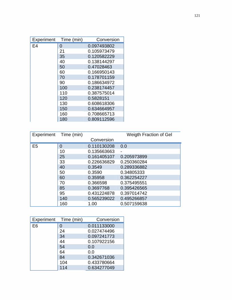
121

Experiment Time (min) Conversion

E4 0 0.097493802 21 0.105973479 35 0.120582229 40 0.138144297 50 0.47028463 60 0.166950143 70 0.178701159 90 0.186634972 100 0.238174457 110 0.387575014 120 0.5828151 130 0.608618306 150 0.634664957 160 0.708665713 180 0.809112596

Experiment Time (min) Conversion

Weigth Fraction of Gel

E5 0 0.110130208 0.0 10 0.135663663 - 25 0.161405107 0.205973899 33 0.226636829 0.250360284 40 0.3549 0.289336882 50 0.3590 0.34805333 60 0.35958 0.362254227 70 0.366598 0.375495551 85 0.3697768 0.395426565 95 0.431224878 0.397014742 140 0.565239022 0.495266857 160 1.00 0.507159638

Experiment Time (min) Conversion

E6 0 0.011133000 24 0.027474496 34 0.097241773 44 0.107922156 54 0.0 64 0.0 84 0.342671036 104 0.433780664 114 0.634277049

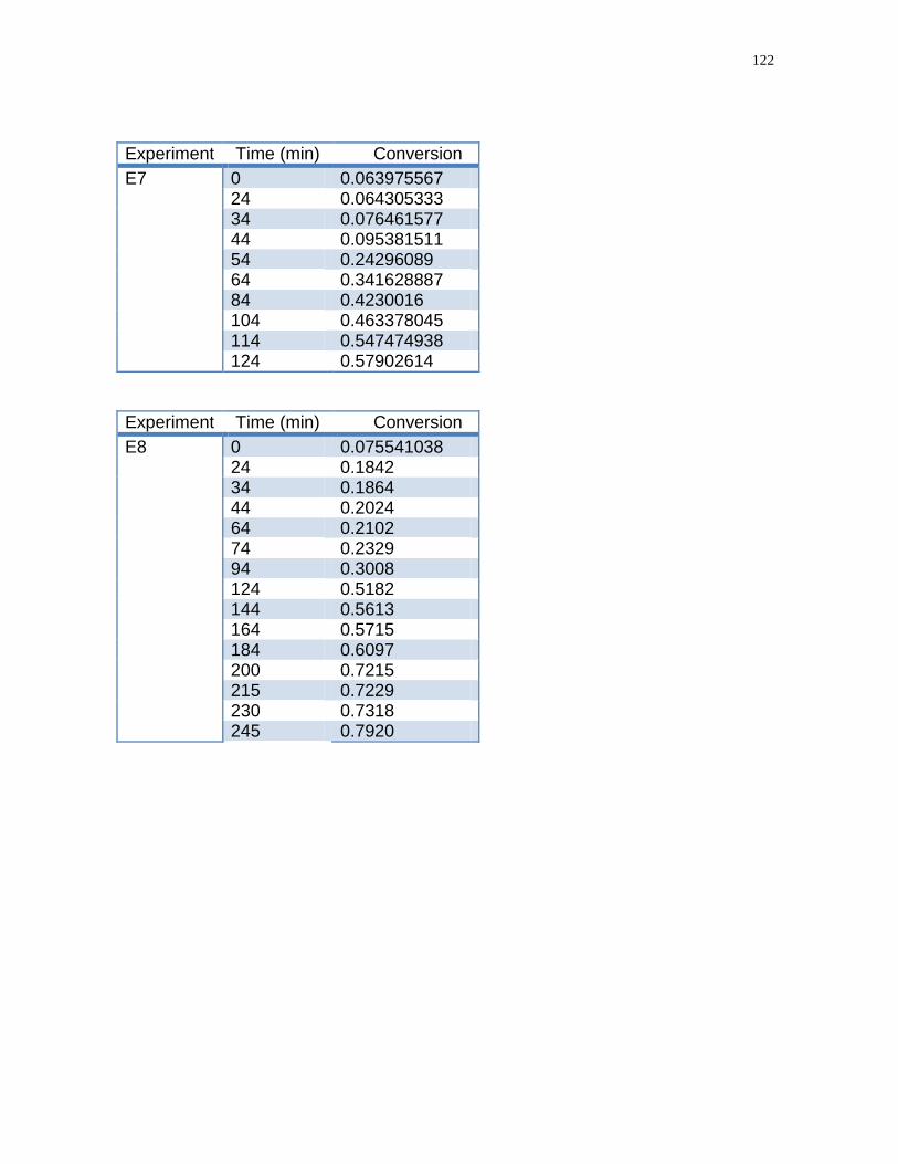
122

Experiment Time (min) Conversion

E7 0 0.063975567 24 0.064305333 34 0.076461577 44 0.095381511 54 0.24296089 64 0.341628887 84 0.4230016 104 0.463378045 114 0.547474938 124 0.57902614

Experiment Time (min) Conversion

E8 0 0.075541038 24 0.1842 34 0.1864 44 0.2024 64 0.2102 74 0.2329 94 0.3008 124 0.5182 144 0.5613 164 0.5715 184 0.6097 200 0.7215 215 0.7229 230 0.7318 245 0.7920

123

Experiment Time (min) Conversion

E9 0 0.0079266 24 0.012491 34 0.029973 44 0.033147 64 0.057132 74 0.06973 94 0.088701 124 0.10001 144 0.10216 164 0.14806 184 0.3481 200 0.46328 215 0.643 230 0.76442 245 0.80349

Experiments

Time (min) Conversion

Weigth Fraction of Gel

E10 0 0.029586 0.0 10 0.0842579 0.15421458 25 0.186918 0.239066402 33 0.1889047 0.283167632 40 0.4311739 0.334243273 50 0.4473012 0.376115165 60 0.5225997 0.408828547 70 0.676308 0.462585507 85 0.6877301 0.512871323 95 0.7147112 0.541705286 140 0.9177995 0.609218052

124

Experiment Time (min) Conversion

E11 0 0.1479 10 0.1499 20 0.2369 30 0.3696 40 0.3960 50 0.4560 60 0.4857 70 0.5116 80 0.5177 90 0.5234 100 0.5793 110 0.5994 120 0.6835 135 0.6841 145 0.6874 150 0.7095 170 0.7980 180 0.8139 200 0.8268 220 0.9827

Experiment Time (min) Conversion

E12 0 0.01432 30 0.04389 45 0.07369 55 0.1295 65 0.2332 75 0.26417 85 0.28303 95 0.33943 100 0.40235 105 0.41775 115 0.43712 120 0.45419 135 0.54149 145 0.69996 155 0.75782

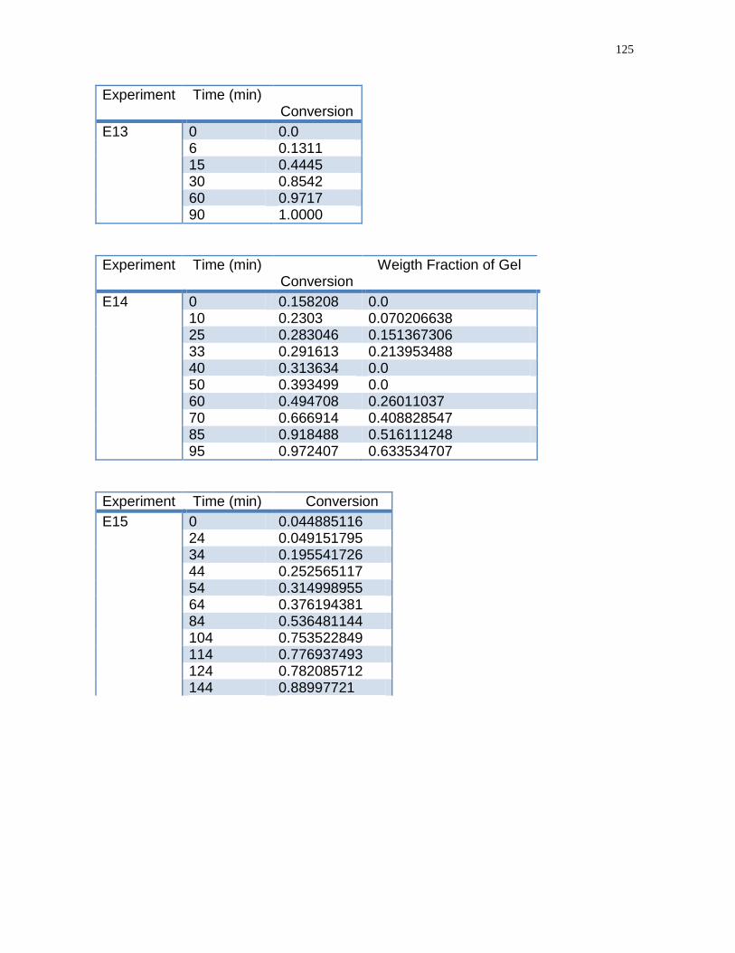
125

Experiment Time (min) Conversion

E13 0 0.0 6 0.1311 15 0.4445 30 0.8542 60 0.9717 90 1.0000

Experiment Time (min) Conversion

Weigth Fraction of Gel

E14 0 0.158208 0.0 10 0.2303 0.070206638 25 0.283046 0.151367306 33 0.291613 0.213953488 40 0.313634 0.0 50 0.393499 0.0 60 0.494708 0.26011037 70 0.666914 0.408828547 85 0.918488 0.516111248 95 0.972407 0.633534707

Experiment Time (min) Conversion

E15 0 0.044885116 24 0.049151795 34 0.195541726 44 0.252565117 54 0.314998955 64 0.376194381 84 0.536481144 104 0.753522849 114 0.776937493 124 0.782085712 144 0.88997721

126

Experiment Time (min) Conversion

E16 0 0.11208225 24 0.23545104 34 0.27415721 44 0.54802538 64 0.55974058 74 0.74926421 94 0.88681986 124 0.9381462 144 0.96539589 164 0.99786944

Experiment Time (min) Conversion

E17 0 0.0717 24 0.08501 34 0.11924 44 0.29743 54 0.33762 64 0.69662 104 0.77036 134 0.7874 154 0.17967 174 0.83599

Experiment Time (min) Conversion

E18 0 0.12922563 24 0.1358834 34 0.16865779 44 0.1778416 54 0.22123919 64 0.3552454 104 0.57347872 134 0.73470495 154 0.759961 174 0.77686238

127

APPENDICE C- MATLAB CODE

Condições iniciais % I AA TMPTA (mol/L) CI=[0.020207 2.055 0.0004261];

% TC=50 ; %Temperatura em °C TC=60 ; %Temperatura em °C % TC=70 ; %Temperatura em °C fsol= 0.0 ; %Fração solúvel de oxigênio (inibidor) em relação ao

equilíbrio a 17°C

% Resultados Experimentais

% Conversão de monômero

% % % % %(min) X % conv1=[ 0 0.043249056 % 24 0.012490692 % 34 0.088700536 % 44 0.100011691 % 54 0.102162219 % 74 0.148058148 % 84 0.463276812 % 104 0.764417248 % 114 0.993500687];

% % % % % (min) X % conv2=[0 0.251331285 % 24 0.26842 % 34 0.27823918 % 44 0.369273455 % 54 0.405575175 % 64 0.48117 % 84 0.880286592];

128

% % % % %(min) X % conv3=[ 0 0.097795456 % 24 0.126431666 % 34 0.091220091 % 44 0.12666868 % 64 0.114684696 % 74 0.148845114 % 94 0.118550449 % 124 0.07202903 % 144 0.07182901 % 164 0.086728234 % 184 0.124342619 % 200 0.284232218 % 215 0.44624250 % 230 0.622375982 % 245 0.684803436];

% % (min) X % % conv4=[ 0 0.097493802 % 21 0.105973479 % 35 0.120582229 % 40 0.138144297 % 50 0.47028463 % 60 0.166950143 % 70 0.178701159 % 90 0.186634972 % 100 0.238174457 % 110 0.387575014 % 120 0.5828151 % 130 0.608618306 % 150 0.634664957 % 160 0.708665713 % 180 0.809112596];

% % (min) X % conv5=[0 0.110130208 % 10 0.135663663 % 25 0.161405107 % 33 0.226636829 % 40 0.3549 % 50 0.3590 % 60 0.35958 % 70 0.366598 % 85 0.3697768 % 95 0.431224878 % 140 0.565239022 % 160 1.00]; %

129

% % % % % (min) X % conv6=[%0 0.011133000 % 24 0.027474496 % 34 0.097241773 % 44 0.107922156 % %54 0.0 % %64 0.0 % 84 0.342671036 % 104 0.433780664 % 114 0.634277049]; %

% % (min) X % conv7=[ 0 0.063975567 % 24 0.064305333 % 34 0.076461577 % 44 0.095381511 % 54 0.24296089 % 64 0.341628887 % 84 0.4230016 % 104 0.463378045 % 114 0.547474938 % 124 0.57902614];

% % % % (min) X % conv8=[ 0 0.075541038 % 24 0.1842 % 34 0.1864 % 44 0.2024 % 64 0.2102 % 74 0.2329 % 94 0.3008 % 124 0.5182 % 144 0.5613 % 164 0.5715 % 184 0.6097 % 200 0.7215 % 215 0.7229 % 230 0.7318 % 245 0.7920];

%

130

% % (min) X % conv9=[0 0.0079266 % 24 0.012491 % 34 0.029973 % 44 0.033147 % 64 0.057132 % 74 0.06973 % 94 0.088701 % 124 0.10001 % 144 0.10216 % 164 0.14806 % 184 0.3481 % 200 0.46328 % 215 0.643 % 230 0.76442 % 245 0.80349];

% % % (min) X % conv10=[ 0 0.029586 % 10 0.0842579 % 25 0.186918 % 33 0.1889047 % 40 0.4311739 % 50 0.4473012 % 60 0.5225997 % 70 0.676308 % 85 0.6877301 % 95 0.7147112 % 140 0.9177995];

% % % (min) X % conv11=[ 0 0.1479 % 10 0.1499 % 20 0.2369 % 30 0.3696 % 40 0.3960 % 50 0.4560 % 60 0.4857 % 70 0.5116 % 80 0.5177 % 90 0.5234 % 100 0.5793 % 110 0.5994 % 120 0.6835 % 135 0.6841 % 145 0.6874 % 150 0.7095 % 170 0.7980 % 180 0.8139 % 200 0.8268 % 220 0.9827 ];

131

% % % % %(min) X % conv12=[ 0 0.01432 % 30 0.04389 % 45 0.07369 % 55 0.1295 % 65 0.2332 % 75 0.26417 % 85 0.28303 % 95 0.33943 % 100 0.40235 % 105 0.41775 % 115 0.43712 % 120 0.45419 % 135 0.54149 % 145 0.69996 % 155 0.75782];

% % (min) X % % conv13=[ 0 0.0 % % 6 0.1311 % % 15 0.4445 % % 30 0.8542 % % 60 0.9717 % % 90 1.0000];

% % % % (min) X % conv14=[ 0 0.158208 % 10 0.2303 % 25 0.283046 % 33 0.291613 % 40 0.313634 % 50 0.393499 % 60 0.494708 % 70 0.666914 % 85 0.918488 % 95 0.972407 ];

% % % % % % % (min) X % conv15=[ 0 0.044885116 % 24 0.049151795 % 34 0.195541726 % 44 0.252565117 % 54 0.314998955 % 64 0.376194381 % 84 0.536481144 % 104 0.753522849 % 114 0.776937493 % 124 0.782085712 % 144 0.88997721];

132

% % % % % (min) X % conv16=[0 0.11208225 % 24 0.23545104 % 34 0.27415721 % 44 0.54802538 % 64 0.55974058 % 74 0.74926421 % 94 0.88681986 % 124 0.9381462 % 144 0.96539589 % 164 0.99786944];

% % % % % % (min) X % conv17=[ 0 0.0717 % 24 0.08501 % 34 0.11924 % 44 0.29743 % 54 0.33762 % 64 0.69662 % 104 0.77036 % 134 0.7874 % 154 0.17967 % 174 0.83599];

% % % % % % % (min) X % conv18=[0 0.12922563 % 24 0.1358834 % 34 0.16865779 % 44 0.1778416 % 54 0.22123919 % 64 0.3552454 % 104 0.57347872 % 134 0.73470495 % 154 0.759961 % 174 0.77686238]; %

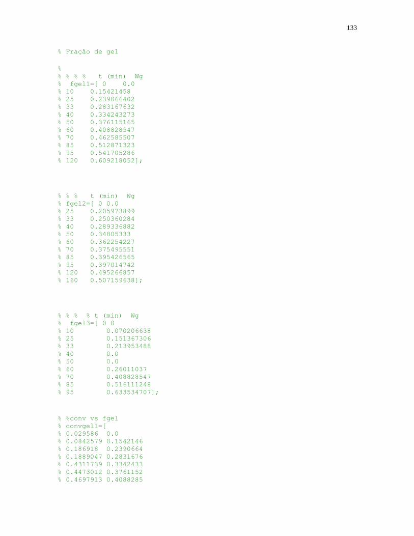
133

% Fração de gel

% % % % % t (min) Wg % fgel1=[ 0 0.0 % 10 0.15421458 % 25 0.239066402 % 33 0.283167632 % 40 0.334243273 % 50 0.376115165 % 60 0.408828547 % 70 0.462585507 % 85 0.512871323 % 95 0.541705286 % 120 0.609218052];

% % % t (min) Wg % fgel2=[ 0 0.0 % 25 0.205973899 % 33 0.250360284 % 40 0.289336882 % 50 0.34805333 % 60 0.362254227 % 70 0.375495551 % 85 0.395426565 % 95 0.397014742 % 120 0.495266857 % 160 0.507159638];

% % % % t (min) Wg % fgel3=[ 0 0 % 10 0.070206638 % 25 0.151367306 % 33 0.213953488 % 40 0.0 % 50 0.0 % 60 0.26011037 % 70 0.408828547 % 85 0.516111248 % 95 0.633534707];

% %conv vs fgel % convgel1=[ % 0.029586 0.0 % 0.0842579 0.1542146 % 0.186918 0.2390664 % 0.1889047 0.2831676 % 0.4311739 0.3342433 % 0.4473012 0.3761152 % 0.4697913 0.4088285

134

% 0.5225997 0.4625855 % 0.676308 0.5128713 % 0.6877301 0.5417053 % 0.7147112 0.6092181 % 0.9177995 0.0 % 1.0407176 0.0];

% % % %conv vs fgel % convgel2=[0.110130208 0.0 % 0.135663663 0.2059739 % 0.161405107 0.2503603 % 0.226636829 0.2893369 % 0.354948634 0.3480533 % 0.35904925 0.3622542 % 0.359581545 0.3754956 % 0.366526718 0.3954266 % 0.369776863 0.3970147 % 0.431224878 0.4952669 % 0.565239022 0.5071596 % 1.003378563 0.0];

% % % % % % conv vs fgel % convgel3=[0.158208 0.0 % 0.2303 0.0702066 % 0.283046 0.1513673 % 0.291613 0.2139535 % 0.313634 0.0 % 0.393499 0.2601104 % 0.494708 0.4088285 % 0.666914 0.5161112 % 0.918488 0.6335347 % 0.972407 0.0 % 0.0 0.0 % 0.0 0.0 % 0.0 0.0 % 0.0 0.0 % 0.995762 0.0 % 0.0 0.0];

% Parâmetros cinéticos

n=1; % Número de gerações m=100 ; % Tamanho máximo da sequencia

kp11=5000; % Constante de propagação do AA. (L/mol.s) r21= 1.2987; % Razão de reatividade r21= kp12/kp11 (= 1.2987 ==>

Gonçalves. 2011) r31= 0.2; % Razão de reatividade r31= kp13/kp11 r43= 0.5; % Razão de reatividade r31= kp14/kp13 r2=1; % Razão de reatividade r2= kp2i/kp1i (p/i= 1 a 4) r3= 0.5; % Razão de reatividade r3= kp3i/kp1i (p/i= 1 a 4) r4=0.25; % Razão de reatividade r3= kp4i/kp1i (p/i= 1 a 4) r5= 1; % Razão de reatividade r3= kp5i/kp1i (p/i= 1 a 4)

135

kd=1.433e10*exp(-22600/(1.987*(TC+273.15))); % Constante de

decomposição do iniciador. NPS fe=0.7; % Eficiência do iniciador

(=0.7 ==> Gonçalves. 2011) kfr=0; % Constante de

transferência de cadeia para o polímero. kh=0; % Constante de abstração

de hidrogênio. kz0= 8e5; % Constante de inibição de

radicais primários. kz= kz0; % Constante de inibição de

radicais poliméricos. ktc=5e7; % Constante de terminação

por combinação. ktd=0; % Constante de terminação

por dismutação. kp13c(2)=1e4; % Constante cinética de

ciclização (entre radical de AA e D3 separados por 2 unidades

monoméricas)

136

function dydt=EDOAATMPTA(t,y) global n m

%Variáveis das equações

DADOSDEFESA %Condições iniciais para Parâmetro Cinéticos

NI=y(1); % Número de mols de iniciador (mol). NM1=y(2); % Número de mols do monómero ácido acrilico (AA) (mol). NM2=y(3); % Número de mols do monómero triacrilato trimetilpropano

TMPTA (mol). NZ= y(4); ND3=y(5); % Número de mols de unidades polimericas com duas duplas

ligações pendentes. ND4=y(6); % Número de mols de unidades polimericas com uma dupla

ligação pendente. VQ0T=y(7); % variável referente ao polímero de ordem o. VQ1T=y(8); % Variável referente ao polímero de ordem 1. VQ00=y(9); %Variável referente ao polímero morto de ordem 0 e geração

0. VQ01=y(10); % Variável referente ao polímero morto de ordem 1 e geração

0. VQ02=y(11); % Variável referente ao polímero morto de ordem 2 e geração

0. V=y(12); % Volume.

for i=1:n

VQ0(i)=y(12+i); % Variável referente ao polímero morto de ordem

0 e geração de 1 a n. VQ1(i)=y(12+n+i); % Variável referente ao polímero morto de ordem

1 e geração de 1 a n. VQ2(i)=y(12+2*n+i); % variável referente ao polímero morto de ordem

2 e geração de 1 a n. Q0(i)=VQ0(i)/V; Q1(i)=VQ1(i)/V; Q2(i)=VQ2(i)/V; end

M1= NM1/V; M2= NM2/V; Z= NZ/V; D3= ND3/V; D4= ND4/V; Q0T=VQ0T/V; Q1T=VQ1T/V; Q00=VQ00/V; Q01=VQ01/V; Q02=VQ02/V; I=NI/V;

M=M1+M2; D=D3+D4;

137

kp12=r21*kp11; % Constante de propagação do TMPTA. kp13=r31*kp11; kp14=r43*kp13; kp21= r2*kp11; kp22= r2*kp12; kp23= r2*kp13; kp24= r2*kp14; kp31= r3*kp11; kp32= r3*kp12; kp33= r3*kp13; kp34= r3*kp14; kp41= r4*kp11; kp42= r4*kp12; kp43= r4*kp13; kp44= r4*kp14; kp51= r5*kp11; kp52= r5*kp12; kp53= r5*kp13; kp54= r5*kp14;

kp14c(2)=(kp14/kp13)*(kp13c(2)); kp23c(2)=(kp23/kp13)*(kp13c(2)); kp24c(2)=(kp24/kp13)*(kp23c(2)); kp33c(2)=(kp33/kp13)*(kp13c(2)); kp34c(2)=(kp34/kp13)*(kp33c(2)); kp43c(2)=(kp43/kp13)*(kp13c(2)); kp44c(2)=(kp44/kp13)*(kp43c(2)); kp53c(2)=(kp53/kp13)*(kp13c(2)); kp54c(2)=(kp54/kp13)*(kp53c(2));

for r= 2:m kp13c(r)= ((1/(r-1))^1.5)*kp13c(2); kp14c(r)= ((1/(r-1))^1.5)*kp14c(2); kp23c(r)= ((1/(r-1))^1.5)*kp23c(2); kp24c(r)= ((1/(r-1))^1.5)*kp24c(2); kp33c(r)= ((1/(r-1))^1.5)*kp33c(2); kp34c(r)= ((1/(r-1))^1.5)*kp34c(2); kp43c(r)= ((1/(r-1))^1.5)*kp43c(2); kp44c(r)= ((1/(r-1))^1.5)*kp44c(2); kp53c(r)= ((1/(r-1))^1.5)*kp53c(2); kp54c(r)= ((1/(r-1))^1.5)*kp54c(2); end

%Constantes das equações ki1=kp11; % A taxa de consumo e

produção de radicais são praticamente iguais no estado pseudo-

estacionário. ki2=kp12; % A taxa de consumo e

produção de radicais são praticamente iguais no estado pseudo-

estacionário. ki3=kp13; ki4=kp14;

138

kt=ktc+ktd; kfr1=kfr; kfr2=kfr; kfr3=kfr; kfr4=kfr; kfr5=kfr;

%Concentrações Molares

%Fracções de monómeros e radicais

fM1=M1/M; fM2=M2/M;

if D3==0 fd3=0; fs=0; else fd3=D3/D; fs=D/Q1T; end

if D4==0 fd4=0; else fd4=D4/D; end

fi1=-(kp12*M2)-(kp13*D3+kp14*D4)-(kfr1*Q1T)-kz*Z; fi2=-(kp21*M1)-(kp23*D3+kp24*D4)-(kfr2*Q1T)-kz*Z; fi3=-(kp31*M1+kp32*M2)-(kp34*D4)-(kfr3*Q1T)-kz*Z; fi4=-(kp41*M1+kp42*M2)-(kp43*D3)-(kfr4*Q1T)-kz*Z; fi5=-(kp51*M1+kp52*M2)-(kp53*D3+kp54*D4)-kz*Z;

YR=[0;0;0;0;1]; XR=[ fi1 M1*kp21 M1*kp31 M1*kp41 M1*kp51 M2*kp12 fi2 M2*kp32 M2*kp42 M2*kp52 D3*kp13 D3*kp23 fi3 D3*kp43 D3*kp53 D4*kp14 D4*kp24 D4*kp34 fi4 D4*kp54 1 1 1 1 1 ];

Br=XR\YR;

fr1=Br(1); fr2=Br(2); fr3=Br(3); fr4=Br(4); fr5=Br(5);

kp=(fr1*(kp11*fM1+kp12*fM2))+(fr2*(kp21*fM1+kp22*fM2))+(fr3*(kp31*fM1+kp3

2*fM2))+(fr4*(kp41*fM1+kp42*fM2))+(fr5*(kp51*fM1+kp52*fM2));

139

ki=(ki1*fM1)+(ki2*fM2);

kpd=((kp13*fd3+kp14*fd4)*fs*fr1)+((kp23*fd3+kp24*fd4)*fs*fr2)+((kp33*fd3+

kp34*fd4)*fs*fr3)+((kp43*fd3+kp44*fd4)*fs*fr4)+((kp53*fd3+kp54*fd4)*fs*fr

5); kid=(ki3*fd3+ki4*fd4)*fs;

R0=(2*kd*fe*I)/((ki1*M1)+(ki2*M2)+(ki3*D3)+(ki4*D4)+kh*Q1T+kz0*Z); a=(ktc+ktd); b=kz*Z; c=-((ki*R0*M)+(kid*R0*Q1T)+kh*Q1T*R0); delta=(b^2)-(4*a*c); Y0T=(-b+(delta^(0.5)))/(2*a);

%Método dos caminhos

kp13c(1)=0; kp14c(1)=0; kp23c(1)=0; kp24c(1)=0; kp33c(1)=0; kp34c(1)=0;

R1= Y0T*fr1; R2= Y0T*fr2; R3= Y0T*fr3; R4= Y0T*fr4; R5= Y0T*fr5;

% Fração de radicais em caminhos frci

fr= [fr1 fr2 fr3 fr4 fr5]; for i=1:4 frs(i)= fr(i)/(fr1+fr2+fr3+fr4); end

T(1)=((ki2*R0*M2)+(M2*(kp12*R1+kp22*R2+kp32*R3+kp42*R4+kp52*R5))+kfr*Q1T)

/((kp21*M1+kp22*M2)+(kp23*D3+kp24*D4)+(ki3*R0)+(kp13*R1+kp23*R2+kp33*R3+k

p43*R4+kp53*R5)+(kt*(R1+R2+R3+R4+R5))+kz*Z+(kp23c(1))); for r=2:m T(r)=((T(r-

1)*(kp11*frs(1)*M1+kp21*frs(2)*M1+kp31*frs(3)*M1+kp41*frs(4)*M1+kp12*frs(

1)*M2+kp22*frs(2)*M2+kp32*frs(3)*M2+kp42*frs(4)*M2+kp13*frs(1)*D3+kp23*fr

s(2)*D3+kp33*frs(3)*D3+kp43*frs(4)*D3+kp14*frs(1)*D4+kp24*frs(2)*D4+kp34*

frs(3)*D4+kp44*frs(4)*D4)))/((kp11*fr1*M1+kp21*fr2*M1+kp31*fr3*M1+kp41*fr

4*M1+kp12*fr1*M2+kp22*fr2*M2+kp32*fr3*M2+kp42*fr4*M2)+(kp13*frs(1)*D3+kp2

3*frs(2)*D3+kp33*frs(3)*D3+kp43*frs(4)*D3+kp14*frs(1)*D4+kp24*frs(2)*D4+k

p34*frs(3)*D4+kp44*frs(4)*D4)+(ki3*R0)+(kp13*R1+kp23*R2+kp33*R3+kp43*R4+k

p53*R5)+(kt*(R1+R2+R3+R4+R5))+kz*Z+(frs(1)*kp13c(r)+frs(2)*kp23c(r)+frs(3

)*kp33c(r)+frs(4)*kp43c(r))); end % CORRIGIR! (Não existe caminho contendo R5) for r=1:m

140

RCD3r(r)= (kp13c(r)*fr1+kp23c(r)*fr2+kp33c(r)*fr3+kp43c(r)*fr4)*T(r); end RCD3=sum(RCD3r);

L(1)=((ki3*R0*D3)+(D3*(kp13*R1+kp23*R2+kp33*R3+kp43*R4+kp53*R5))+(RCD3))/

((kp31*M1+kp32*M2)+(kp33*D3+kp34*D4)+(ki4*R0)+(kp14*R1+kp24*R2+kp34*R3+kp

44*R4+kp54*R5)+(kt*(R1+R2+R3+R4+R5))+kz*Z+(kp34c(1))); for r=2:m L(r)=((L(r-

1)*((kp11*fr1*M1+kp21*fr2*M1+kp31*fr3*M1+kp41*fr4*M1+kp51*fr5*M1+kp12*fr1

*M2+kp22*fr2*M2+kp32*fr3*M2+kp42*fr4*M2+kp52*fr4*M2)+(kp13*fr1*D3+kp23*fr

2*D3+kp33*fr3*D3+kp43*fr4*D3+kp53*fr5*D3+kp14*fr1*D4+kp24*fr2*D4+kp34*fr3

*D4+kp44*fr4*D4+kp54*fr5*D4))))/((kp11*frs(1)*M1+kp21*frs(2)*M1+kp31*frs(

3)*M1+kp41*frs(4)*M1+kp12*frs(1)*M2+kp22*frs(2)*M2+kp32*frs(3)*M2+kp42*fr

s(4)*M2)+(kp13*fr1*D3+kp23*fr2*D3+kp33*fr3*D3+kp43*fr4*D3+kp53*fr5*D3+kp1

4*fr1*D4+kp24*fr2*D4+kp34*fr3*D4+kp44*fr4*D4+kp54*fr5*D4)+(ki4*R0)+(kp13*

R1+kp23*R2+kp33*R3+kp43*R4+kp53*R5)+(kt*(R1+R2+R3+R4+R5))+kz*Z+(fr1*kp14c

(r)+fr2*kp24c(r)+fr3*kp34c(r)+fr4*kp44c(r)+fr5*kp54c(r))); end

for r=1:m RCD4r(r)=

(kp14c(r)*fr1+kp24c(r)*fr2+kp34c(r)*fr3+kp44c(r)*fr4+kp54c(r)*fr5)*L(r); end RCD4=sum(RCD4r);

%Balanço Volumétrico

densu=1150; %g/L densm=1050; %g/L

dVdt=(ki*R0*M+kp*Y0T*M)*72.06*V*((1/(densu))-(1/(densm)));

%Balanços de espécies

dNIdt=(-kd*I)*V;

% Balanço ao iniciador. dNM1dt=((ki1*R0*M1)-((kp11*R1+kp21*R2+kp31*R3+kp41*R4+kp51*R5)*M1))*V;%

Balanço ao ácido acrilíco. dNM2dt=((ki2*R0*M2)-((kp12*R1+kp22*R2+kp32*R3+kp42*R4+kp52*R5)*M2))*V;

% Balanço ao TMPTA. dNZdt= -(kz0*R0*Z+kz*Y0T*Z)*V; dND3dt=((ki2*R0*M2)+(((kp12*R1)+(kp22*R2)+(kp32*R3)+(kp42*R4)+(kp52*R5))*

M2)-(ki3*R0*D3)-(((kp13*R1)+(kp23*R2)+(kp33*R3)+(kp43*R4)+(kp53*R5))*D3)-

RCD3)*V; % Balanço as unidades polimericas com duas duplas pendentes. dND4dt=((ki3*R0*D3)-(ki4*R0*D4)-

(((kp14*R1)+(kp24*R2)+(kp34*R3)+(kp44*R4)+(kp54*R5))*D4)+(((kp13*R1)+(kp2

3*R2)+(kp33*R3)+(kp43*R4)+(kp53*R5))*D3)-RCD4+RCD3)*V; % Balanço as

unidades poliméricas com uma dupla pendente. dVQ0Tdt=(-(kid*R0*Q1T)-(kpd*Y0T*Q1T)-

(kh*Q1T*R0)+((ktc/2)*(Y0T^2))+((ktd*(Y0T^2)))+kz*Y0T*Z)*V; dVQ1Tdt=(ki*R0*M+kp*Y0T*M)*V;

141

if Q01==0; Q03=0; else Q03= (2*(Q02^2)/(Q01))-((Q02*Q01)/Q00); end

for i=1:n if Q1(i)==0 Q3(i)=0; else Q3(i)=((2*((Q2(i))^2))/(Q1(i)))-((Q2(i)*Q1(i))/Q0(i)); end end

%Geração 0

Y00=(ki*R0*M)/((kfr*Q1T)+(kpd*Q1T)+(kt*Y0T)+kz*Z); Y01=((ki*R0*M)+(kp*Y00*M))/((kfr*Q1T)+(kpd*Q1T)+(kt*Y0T)+kz*Z); Y02=((ki*R0*M)+(kp*M*(2*Y01+Y00)))/((kt*Y0T)+(kpd*Q1T)+(kfr*Q1T)+kz*Z); dVQ00dt=(-(kid*R0*Q01)-(kpd*Y0T*Q01)-(kfr*(Q01*Y0T-Q1T*Y00))-

(kh*Q01*R0)+((ktc*(Y00^2))/2)+(ktd*Y00*Y0T)+kz*Y00*Z)*V; dVQ01dt=(-(kid*R0*Q02)-(kpd*Y0T*Q02)-(kfr*(Q02*Y0T-Q1T*Y01))-

(kh*Q02*R0)+(ktc*Y01*Y00)+(ktd*Y01*Y0T)+kz*Y01*Z)*V; dVQ02dt=(-(kid*R0*Q03)-(kpd*Y0T*Q03)-(kfr*Y0T*Q03)+(kfr*Q1T*Y02)-

(kh*Q03*R0)+(ktc*(Y02*Y00+Y01^2))+(ktd*Y02*Y0T)+kz*Y02*Z)*V;

%Geração 1

Y0(1)=((kid*R0*Q01)+(Y00*(kpd*(Q01+Q1(1))))+(kfr*Y0T*Q01)+(kfr*Y0T*Q1(1))

+(kh*R0*(Q01+Q1(1)))+(kid*R0*Q1(1)))/(kpd*(Q1T-

Q01)+(kfr*Q1T)+((ktc+ktd)*Y0T)+kz*Z); Y1(1)=((kp*Y0(1)*M)+(kfr*(Y0T*Q02+Y0T*Q2(1)))+kh*(R0*Q02+R0*Q2(1))+kid*R0

*(Q02+Q2(1))+kpd*(Q02*Y00+Q01*Y01+Q02*Y0(1)+Q2(1)*Y00+Q1(1)*Y01))/((kpd*(

Q1T-Q01)+kfr*Q1T+(ktc+ktd)*Y0T)+kz*Z); Y2(1)=((kp*M*(2*Y1(1)+Y0(1)))+(kfr*Y0T*(Q03+Q3(1)))+kh*R0*(Q03+Q3(1))+(ki

d*R0*(Q03+Q3(1)))+(kpd*(Q03*Y00+2*Q02*Y01+Q01*Y02+Q03*Y0(1)+2*Q02*Y1(1)+Q

3(1)*Y00+2*Q2(1)*Y01+Q1(1)*Y02)))/(kpd*(Q1T-Q01)+kfr*Q1T+kt*Y0T+kz*Z); dVQ0dt(1)=(-(kid*R0*Q1(1))-(kpd*Y0T*Q1(1))-(kfr*(Q1(1)*Y0T-Q1T*Y0(1)))-

(kh*Q1(1)*R0)+(ktc*Y00*Y0(1))+(ktd*Y0(1)*Y0T)+kz*Y0(1)*Z)*V; dVQ1dt(1)=(-(kid*R0*Q2(1))-(kpd*Y0T*Q2(1))-(kfr*(Q2(1)*Y0T-Q1T*Y1(1)))-

(kh*Q2(1)*R0)+(ktc*Y1(1)*Y00)+(ktc*Y0(1)*Y01)+(ktd*Y1(1)*Y0T)+kz*Y1(1)*Z)

*V; dVQ2dt(1)=(-(kid*R0*Q3(1))-(kpd*Y0T*Q3(1))-

(kfr*Y0T*Q3(1))+(kfr*Q1T*Y2(1))-

(kh*Q3(1)*R0)+(ktc*(Y02*Y0(1)+2*Y01*Y1(1)+Y00*Y2(1)))+(ktd*Y2(1)*Y0T)+kz*

Y2(1)*Z)*V;

142

%Geração i

for i=2:n

Y0(i)=(kfr*Q1(i)*Y0T+kh*R0*Q1(i)+kpd*Y0(i-1)*Q1(i-

1)+kpd*Q1(i)*(Y00+sum(Y0(1:i-1)))+(kid*R0*Q1(i)))/(kpd*(Q1T-

(Q01+sum(Q1(1:i-1))))+kfr*Q1T+kt*Y0T+kz*Z); Y1(i)=(kp*Y0(i)*M+kfr*Q2(i)*Y0T+kh*R0*Q2(i)+kpd*(Q2(i-1)*Y0(i-1)+Q1(i-

1)*Y1(i-1)+Y0(i)*(Q02+sum(Q2(1:i-1)))+Q2(i)*(Y00+sum(Y0(1:i-

1)))+Q1(i)*(Y01+sum(Y1(1:i-1))))+kid*R0*Q2(i))/(kpd*(Q1T-(Q01+sum(Q1(1:i-

1))))+kfr*Q1T+kt*Y0T+kz*Z); Y2(i)=(kp*M*(2*Y1(i)+Y0(i))+kfr*Q3(i)*Y0T+kh*Q3(i)*R0+kpd*(Q3(i-1)*Y0(i-

1)+2*Q2(i-1)*Y1(i-1)+Y0(i)*(Q03+sum(Q3(1:i-1)))+Q1(i-1)*Y2(i-

1)+2*Y1(i)*(Q02+(sum(Q2(1:i-1))))+Q3(i)*(Y00+sum(Y0(1:i-

1)))+Q1(i)*(Y02+sum(Y2(1:i-1)))+2*Q2(i)*(Y01+sum(Y1(1:i-

1))))+kid*R0*Q3(i))/(kpd*(Q1T-(Q01+sum(Q1(1:i-1))))+kfr*Q1T+kt*Y0T+kz*Z); dVQ0dt(i)=(-(kid*R0*Q1(i))-(kpd*Y0T*Q1(i))-(kfr*(Q1(i)*Y0T-Q1T*Y0(i)))-

(kh*Q1(i)*R0)+ktc*(((Y0(i-1))^2)/2+Y0(i)*(Y00+sum(Y0(1:i-

1))))+ktd*Y0T*Y0(i)+kz*Y0(i)*Z)*V; dVQ1dt(i)=(-(kid*R0*Q2(i))-(kpd*Y0T*Q2(i))-(kfr*(Q2(i)*Y0T-Q1T*Y1(i)))-

(kh*Q2(i)*R0)+ktc*(Y0(i-1)*Y1(i-1)+Y0(i)*(Y01+sum(Y1(1:i-

1)))+Y1(i)*(Y00+sum(Y0(1:i-1))))+(ktd*Y1(i)*Y0T)+kz*Y1(i)*Z)*V; dVQ2dt(i)=(-(kid*R0*Q3(i))-(kpd*Y0T*Q3(i))-(kfr*(Q3(i)*Y0T-Q1T*Y2(i)))-

(kh*Q3(i)*R0)+ktc*(Y0(i-1)*Y2(i-1)+(Y1(i-1))^2+Y0(i)*(Y02+sum(Y2(1:i-

1)))+2*Y1(i)*(Y01+sum(Y1(1:i-1)))+Y2(i)*(Y00+sum(Y0(1:i-

1))))+ktd*Y2(i)*Y0T+kz*Y2(i)*Z)*V; end

dydt=[dNIdt;dNM1dt;dNM2dt;dNZdt;dND3dt;dND4dt;dVQ0Tdt;dVQ1Tdt;dVQ00dt;dVQ

01dt;dVQ02dt;dVdt;dVQ0dt';dVQ1dt';dVQ2dt'];

143

lobal n m clear all clc

DADOSDEFESA

nexps=size(CI);

for k=1:nexps(1)

EXP=CI(k,:);

NIo=EXP(1); NM1o=EXP(2); NM2o=EXP(3); fAA= NM1o*72/1050; mH2O= (((NM1o*72)/1.050)*(1-fAA)/fAA)/1000; %kg SolubO2= 0.00965; % (g O2/kg H2O a 17ºC) NZo= fsol*mH2O*SolubO2/32; % mol ND3o=0; ND4o=0; Q0To=0; Q1To=0; Q00o=0; Q01o=0; Q02o=0; Vo=1; for j=1:n Qi0o(j)=0; Qi1o(j)=0; Qi2o(j)=0; end

intt=[0:1:300]*60;

%Intervalo de tempo da reacção de copolimerização radicalar do AA-TMPTA

(s) f0=[NIo;NM1o;NM2o;NZo;ND3o;ND4o;Q0To;Q1To;Q00o;Q01o;Q02o;Vo;Qi0o';Qi1o';Q

i2o']; %Condições iniciais dos componentes da

reacção %ode45('cop',intt,f0); [t,f]=ode45('EDOAATMPTA',intt,f0);

NI=f(:,1); NM1=f(:,2); NM2=f(:,3); NZ=f(:,4); ND3=f(:,5); ND4=f(:,6); Q0T=f(:,7); Q1T=f(:,8); Q00=f(:,9); Q01=f(:,10); Q02=f(:,11); V=f(:,12);

144

for j=1:n Q0(:,j)=f(:,12+j); Q1(:,j)=f(:,12+n+j); Q2(:,j)=f(:,12+2*n+j); end

for i=1:length(NI) X(i,k)=((NM1o+NM2o)-(NM1(i)+NM2(i)))/(NM1o+NM2o); % Mn(i)=(Q01(i)+sum(Q1(i,:)))*72.06/(Q00(i)+sum(Q0(i,:))); % Mw(i)=(Q02(i)+sum(Q2(i,:)))*72.06/(Q01(i)+sum(Q1(i,:))); % Mw0(i)=(Q02(i))*72.06/(Q01(i)); % Mw1(i)=(Q2(i,1))*72.06/((Q1(i,1))); % Mw2(i)=(Q2(i,2))*72.06/((Q1(i,2))); % Mw3(i)=(Q2(i,3))*72.06/((Q1(i,3))); % Mw4(i)=(Q2(i,4))*72.06/((Q1(i,4))); %Mw5(i)=(Q2(i,5))*72.06/((Q1(i,5))); Wg(i,k)=(Q1T(i)-(Q01(i)+sum(Q1(i,:))))/Q1T(i); end

end % % [Q1T Q01 Q1]

tmin=intt/60;

%figure (6) %x= %curva de ajuste pontos experimentais %x = lsqcurvefit(@myfun,x0,xdata,ydata) %where myfun is a MATLAB function such as %function F = myfun(x,xdata) %F = ... % Compute function values at x, xdata %fun can also be a function handle for an anonymous function. %f = @(x,xdata)x(1)*xdata.^2+x(2)*sin(xdata); %x = lsqcurvefit(f,x0,xdata,ydata); %hold all

% % % Figure(8) subplot(1,2,2) plot(fgel1(:,1), fgel1(:,2),'s',tmin,Wg,'-') hold all

% % % figure (6) % subplot(1,2,1) % plot(conv17(:,1), conv17(:,2),'s',tmin,X,'-') % hold all

% figure(82) % subplot(1,2,2) % plot(convgel2(:,1), convgel2(:,2),'s',X,Wg,'-') % plot(convgel3(:,1), convgel3(:,2),'s',X,Wg,'-') % hold all