POLYNOMIAL PATTERNS Learning Task:1. In the activation activity, we looked at four different polynomial functions. a. Let’s break down the word: poly- and –nomial. What does “poly” mean? b. A monomial is a numeral, variable, or the product of a numeral and one or more variables. For example, -1, ½, 3x, and 2xy are monomials. Give a few examples of other monomials: c. What is a constant? Give a few examples: d. e. The degree of a monomial is the sum of the exponents of its variables. The monomial 5x3y has degree 4. Why? What is the degree of the monomial 3? Why? f. The examples shown below are all polynomials. Based on these examples and the definition of a monomial, define polynomial .

2x2 + 3x 4xy3 7x5 18x3 + 2x2 – 3x + 5

A coefficient is the numerical factor of a monomial or the ___________ in front of the variable in a monomial. Give some examples of monomials and their coefficients.

Monomial Coefficient

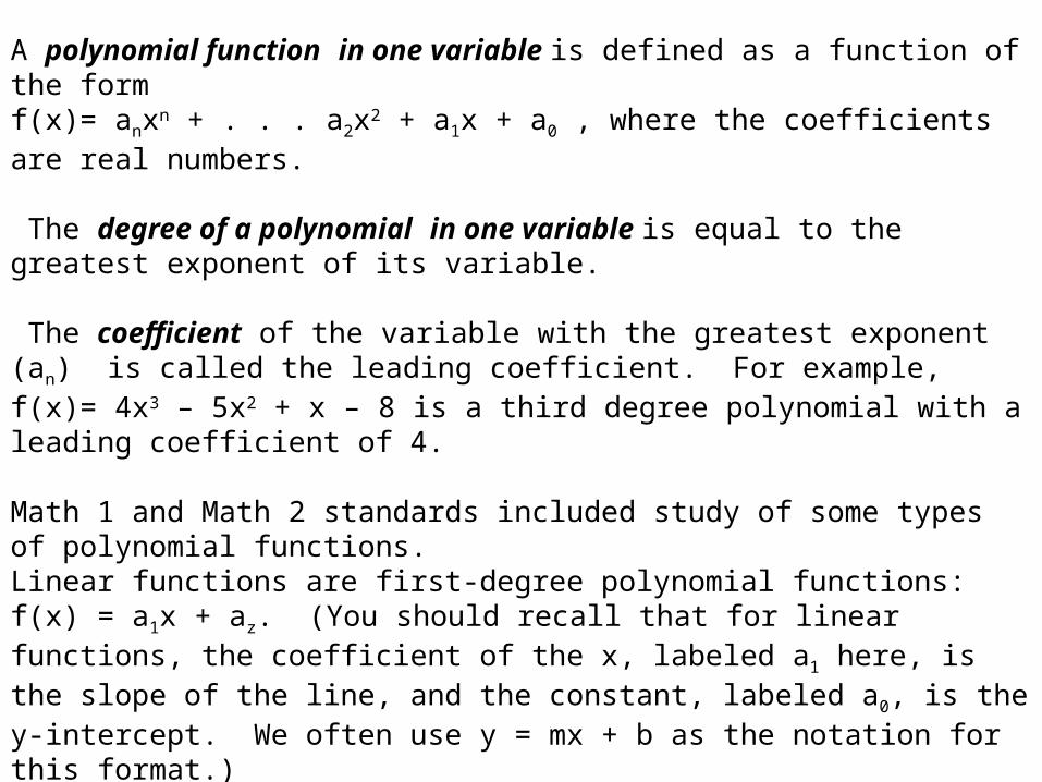
A polynomial function in one variable is defined as a function of the formf(x)= anxn + . . . a2x2 + a1 x + a0 , where the coefficients are real numbers.

The degree of a polynomial in one variable is equal to the greatest exponent of its variable.

The coefficient of the variable with the greatest exponent (an) is called the leading coefficient. For example, f(x)= 4x3 – 5x2 + x – 8 is a third degree polynomial with a leading coefficient of 4. Math 1 and Math 2 standards included study of some types of polynomial functions. Linear functions are first-degree polynomial functions: f(x) = a1x + az. (You should recall that for linear functions, the coefficient of the x, labeled a1 here, is the slope of the line, and the constant, labeled a0, is the y-intercept. We often use y = mx + b as the notation for this format.)

Quadratic functions are second-degree polynomial functions: f(x) = a2x2 + a1x + az.Cubic functions are third-degree polynomial functions: f(x) = a3x3 + a2x2 + a1x + az.There are also fourth, fifth, sixth, etc. degree polynomial functions.

2. To get an idea of what these functions look like, we can graph some basic first through fifth degree polynomials with leading coefficients of 1 and constants equal to 0. For each polynomial function, make a table of 6 points and then plot them so that you can determine the shape of the graph. Choose points that are both positive and negative so that you can get a good idea of the shape of the graph. Also, include the x intercept as one of your points.

a. On a sheet of graph paper, write tables and draw graphs for the second-, third-, fourth-, and fifth-degree functions with leading coefficients of 1 and constants equal to 0.

b. By looking at the graphs, describe in your own words how the second-degree function is similar to and how it is different from the fourth-degree function.Describe how the third-degree function is similar to and how it is different from thefifth-degree function.

Note any other observations about how the characteristics of these graphs compare with each other.

For example, for a first order polynomial function with a leading coefficient of 1 and a constant of 0, the function may be written as f(x) = x. A sample table and the graph of the function are shown to the right.

x f(x)-3 -3-1 -10 02 25 5

10 10

3. In this unit, we are going to discover different characteristics of polynomial functions by looking at patterns in their behavior. Polynomials can be classified by the number of monomials, or terms, as well as by the degree of the polynomial. Remember that the degree of the polynomial is the same as that of the term with the highest degree. Complete the following chart. Make up your own expression for the last row.

ExampleDegre

eName (based on degree)

No. of terms

Name (based on

no. of terms)

2 Constant Monomial2x2 + 3 Quadratic Binomial

-x3 Cubicx4 + 3x2 Quartic

3x5 – 4x + 2 Quintic Trinomial

In order to examine their characteristics in detail so that we can find the patterns that arise in the behavior of polynomial functions, we can study some examples of polynomial functions and their graphs. On a separate page are eight polynomial functions and their accompanying graphs that we will use to refer back to throughout the task. Each of these equations is written in the standard polynomial format, then rewritten as a product of linear factors by factoring the equations. Use colored pencils to label the indicated features in the equations and on the graphs.

4. a. For each graph, use the graph to find the x-intercepts of the functions. On the table below, write the x-intercepts of the function in the first column, then write the linear factors of the function in the second column.

How are the intercepts related to the linear factors?

Why might it be useful to know the linear factors of a function?

Functionx-intercepts Linear factors

f(x) = x2 + 2xg(x) = -2x2 + xh(x)= x3 - xj(x) = -x3 + 2x2 + 3xk(x) = x4 – 5x2 + 4l(x) = -(x4 – 5x2 + 4)m(x) = ½(x5+4x4-7x3-22x2+24x) n(x) = -½(x5+4x4-7x3-22x2+24x)

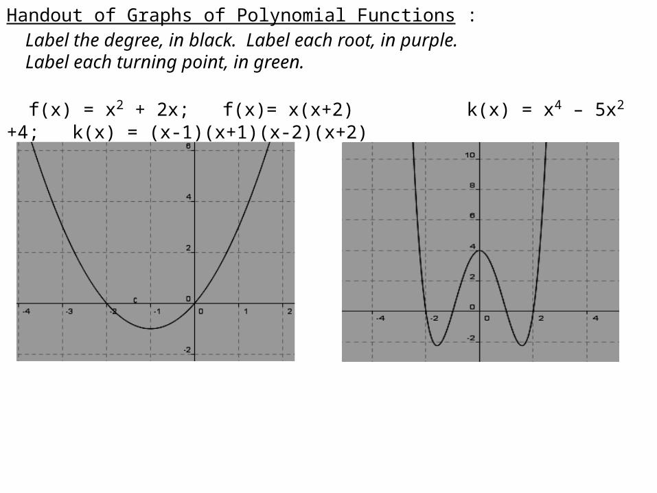
Handout of Graphs of Polynomial Functions : Label the degree, in black. Label each root, in purple. Label each turning point, in green.

f(x) = x2 + 2x; f(x)= x(x+2) k(x) = x4 – 5x2 +4; k(x) = (x-1)(x+1)(x-2)(x+2)

g(x) = -2x2 + x; g(x) = x(-2x+1) l(x) = -(x4 – 5x2 +4); l(x) = -(x-1)(x+1)(x-2)(x+2)

h(x) = x3 – x; m(x) = ½(x5 + 4x4 – 7x3 – 22x2 + 24x) h(x) = x(x – 1)(x + 1) m(x) = ½x(x - 1)(x - 2)(x + 3)(x + 4)

j(x) = -x3 + 2x2 + 3x; n(x) = -½(x5 + 4x4 – 7x3 – 22x2 + 24x) j(x) = -x(x - 3)(x + 1) n(x) = -½x(x – 1)(x – 2)(x + 3)(x + 4)

5. a. Although we will not factor higher order polynomial functions in this unit, you have factored quadratic functions in Math I and Math II. For review, factor the following second degree polynomials, or quadratics.

y = x2 – x – 12 y = x2 + 5x – 6 y = 2x2 – 6x – 10

b. Using these factors, find the roots of these three equations.

c. Use the relationship between the linear factors and x-intercepts to sketch graphs of the three quadratic equations above.

6

4

2

-2

-4

-6

-10 -5 5 10

6

4

2

-2

-4

-6

-10 -5 5 10

6

4

2

-2

-4

-6

-10 -5 5 10

5. d. Although you will not need to be able to find all of the roots of higher order polynomials until a later unit, using what you already know, you can factor some polynomial equations and find their roots in a similar way. Factor y = x5 + x4 – 2x3.

What are the roots of this fifth order polynomial function?

How many roots are there?

Why are there not five roots since this is a fifth degree polynomial? e. For other polynomial functions, we will not be able to draw upon our knowledge of factoring quadratic functions to find zeroes. For example, you may not be able to factor y = x3 + 8x2 + 5x - 14, but can you still find its zeros by graphing it in your calculator? How? What are the zeros of this polynomial function?

In the previous problems, we studied the relationship between x-intercepts and linear factors and comparisons between polynomials of various derees. Using the same eight graphs, the next characteristic of polynomial functions we will consider is symmetry.

In the previous problems, we studied the relationship between x-intercepts and linear factors and comparisons between polynomials of various degrees. Using the same eight graphs, the next characteristic of polynomial functions we will consider is symmetry. 6. a. Sketch a function you have seen before that has symmetry about the y-axis. Describe in your own words what it means to have symmetry about the y-axis.

What do we call a function that has symmetry about the y-axis?

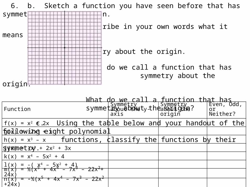
6. b. Sketch a function you have seen before that has symmetry about the origin.

Describe in your own words what it means to have symmetry about the origin.

What do we call a function that has symmetry about the origin?

What do we call a function that has symmetry about the origin?

c. Using the table below and your handout of the following eight polynomial functions, classify the functions by their symmetry.

Function Symmetry about the y-axis

Symmetry about the origin

Even, Odd, or Neither?

f(x) = x2 + 2x

g(x) = -2x2 + x

h(x) = x3 – x

j(x) = -x3 + 2x2 + 3x

k(x) = x4 – 5x2 + 4

l(x) = -( x4 – 5x2 + 4)m(x) = ½(x5 + 4x4 – 7x3 – 22x2+ 24x) n(x) = -½(x5 + 4x4 – 7x3 – 22x2 +24x)

6. d. Sketch your own higher order e. Sketch your own higher order polynomial polynomial function (an equation function with symmetry about the origin. is not needed) with symmetry about the y-axis.

f. Using these examples from the handout and the graphs of the first through fifth degree polynomials you made, why do you think an odd function may be called an odd function? Why are even functions called even functions?

6. g. Why don’t we talk about functions that have symmetry about the x-axis? Sketch a graph that has symmetry about the x-axis. What do you notice?

Another characteristic of functions that you have studied is domain and range. 7. Complete the table below for each of the eight functions.

Function Domain Range

f(x) = x2 + 2x

g(x) = -2x2 + x

h(x) = x3 – x

j(x) = -x3 + 2x2 + 3x

k(x) = x4 – 5x2 + 4

l(x) = -( x4 – 5x2 + 4)m(x) = ½(x5 + 4x4 – 7x3 – 22x2+ 24x) n(x) = -½(x5 + 4x4 – 7x3 – 22x2 +24x)

We can also describe the functions by determining some points on the functions. We can find the x-intercepts for each function as we discussed before. 8. a. For each of the eight functions, write the degree and the ordered pairs of the x-intercepts in the table below.

FunctionDegre

eOrdered pairs of x-intercepts Zeros

Number of

Zerosf(x) = x2 + 2xg(x) = -2x2 + xh(x) = x3 – xj(x) = -x3 + 2x2 + 3xk(x) = x4 – 5x2 + 4l(x) = -( x4 – 5x2 + 4)m(x) = ½(x5 + 4x4 – 7x3 – 22x2+ 24x) n(x) = -½(x5 + 4x4 – 7x3 – 22x2 +24x)

8. b. These x-intercepts are called the zeros of the polynomial functions. Why do you think they have this name? c. Fill in the column labeled “Zeroes” by writing the zeroes that correspond to the x-intercepts of each polynomial function, and also record the number of zeroes each function has. d. Make a conjecture about the relationship of degree of the polynomial and number of zeroes.

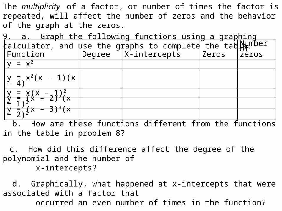
The multiplicity of a factor, or number of times the factor is repeated, will affect the number of zeros and the behavior of the graph at the zeros.

9. a. Graph the following functions using a graphing calculator, and use the graphs to complete the table.

Function Degree X-intercepts ZerosNumber of zeros

y = x2

y = x2(x – 1)(x + 4)y = x(x – 1)2

y = (x – 2)2(x + 1)2

y = (x – 3)3(x + 2)2

b. How are these functions different from the functions in the table in problem 8?

c. How did this difference affect the degree of the polynomial and the number of x-intercepts?

d. Graphically, what happened at x-intercepts that were associated with a factor that occurred an even number of times in the function?

e. Graphically, what happened at x-intercepts that were associated with a factor that occurred an odd number of times in the function?

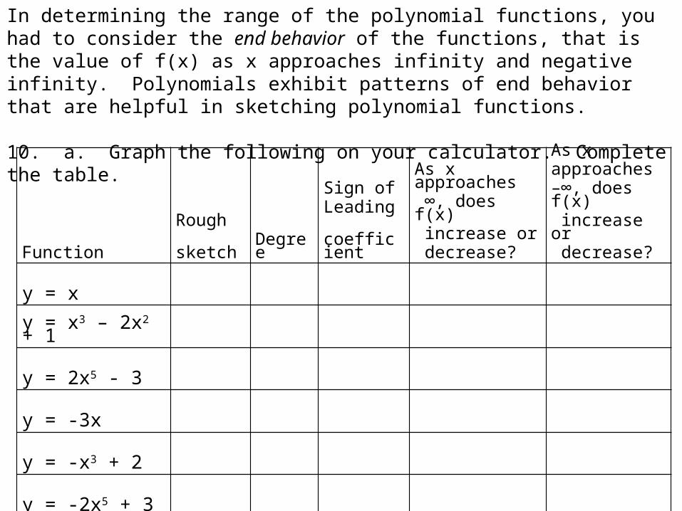
In determining the range of the polynomial functions, you had to consider the end behavior of the functions, that is the value of f(x) as x approaches infinity and negative infinity. Polynomials exhibit patterns of end behavior that are helpful in sketching polynomial functions.

10. a. Graph the following on your calculator. Complete the table.

FunctionRough sketch

Degree

Sign ofLeading coefficient

As x approaches ∞, does f(x) increase or decrease?

As x approaches –∞, does f(x) increase or decrease?

y = x

y = x3 – 2x2 + 1

y = 2x5 - 3

y = -3x

y = -x3 + 2

y = -2x5 + 3

b. Graph the following on your calculator. Complete the table.

FunctionRough sketch

Degree

Sign ofleading Coefficient

As x approaches ∞, does f(x) increase or decrease?

As x approaches -∞, does f(x) increase or decrease?

y = x2

y = -x2 + 2

y = 5x4

y = -3x4

y = x6

y = -2x6

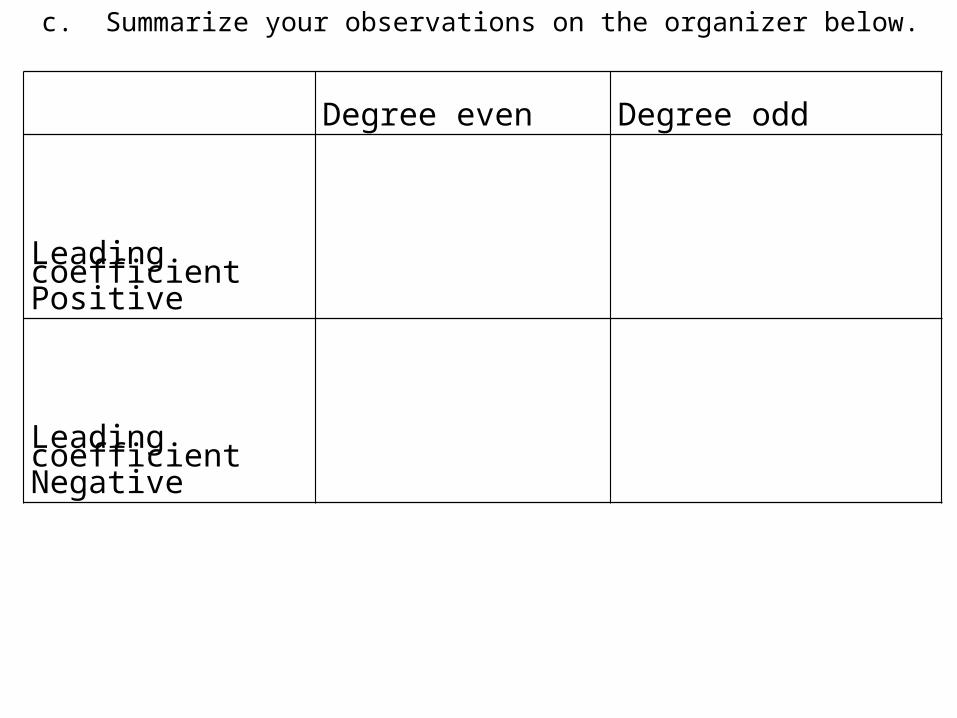
c. Summarize your observations on the organizer below.

Degree even Degree odd

Leading coefficientPositive

Leading coefficient Negative

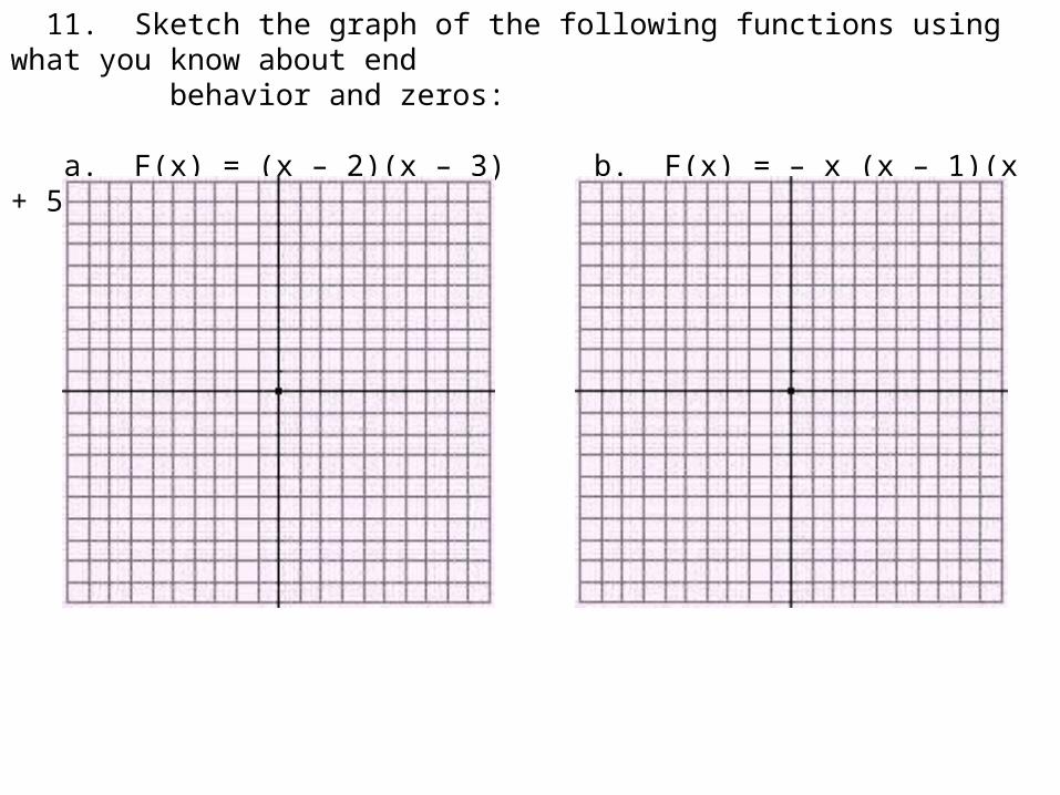
11. Sketch the graph of the following functions using what you know about end behavior and zeros:

a. F(x) = (x – 2)(x – 3) b. F(x) = – x (x – 1)(x + 5)(x – 7)

Other points of interest in sketching the graph of a polynomial function are the points where the graph begins or ends increasing or decreasing.

12. Recall what it means for a point of a function to be an absolute minimum or an absolute maximum.

a. Which of the twelve graphs from problem 10 have an absolute maximum? b. Which have an absolute minimum? c. What do you notice about the degrees of these functions? d. Can you ever have an absolute maximum AND an absolute minimum in the same function? If so, sketch a graph with both. If not, why not?

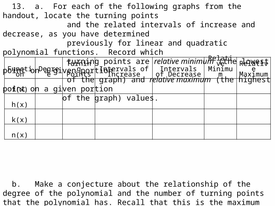
13. a. For each of the following graphs from the handout, locate the turning points and the related intervals of increase and decrease, as you have determined previously for linear and quadratic polynomial functions. Record which turning points are relative minimum (the lowest point on a given portion of the graph) and relative maximum (the highest point on a given portion of the graph) values.

b. Make a conjecture about the relationship of the degree of the polynomial and the number of turning points that the polynomial has. Recall that this is the maximum number of turning points a polynomial of this degree can have because these graphs are examples in which all zeros have a multiplicity of one.

c. Sometimes points that are relative minimums or maximums are also absolute minimums or absolute maximum. Are any of the relative extrema in your table also absolute extrema?

Function

Degree

Turning Points

Intervals of Increase

Intervals of Decrease

Relative Minimu

m

Relative Maximu

m

f(x)

h(x)

k(x)

n(x)