polygonal invariant curves for a planar piecewise...

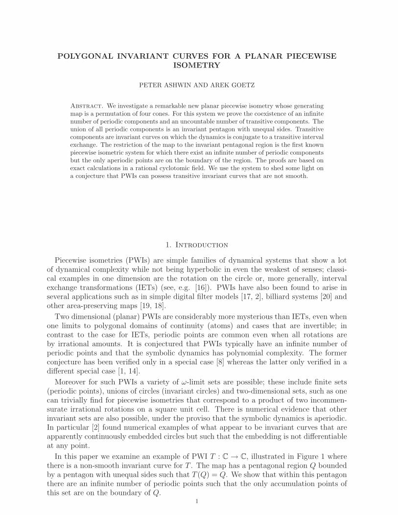
POLYGONAL INVARIANT CURVES FOR A PLANAR PIECEWISEISOMETRY

PETER ASHWIN AND AREK GOETZ

Abstract. We investigate a remarkable new planar piecewise isometry whose generatingmap is a permutation of four cones. For this system we prove the coexistence of an infinitenumber of periodic components and an uncountable number of transitive components. Theunion of all periodic components is an invariant pentagon with unequal sides. Transitivecomponents are invariant curves on which the dynamics is conjugate to a transitive intervalexchange. The restriction of the map to the invariant pentagonal region is the first knownpiecewise isometric system for which there exist an infinite number of periodic componentsbut the only aperiodic points are on the boundary of the region. The proofs are based onexact calculations in a rational cyclotomic field. We use the system to shed some light ona conjecture that PWIs can possess transitive invariant curves that are not smooth.

1. Introduction

Piecewise isometries (PWIs) are simple families of dynamical systems that show a lotof dynamical complexity while not being hyperbolic in even the weakest of senses; classi-cal examples in one dimension are the rotation on the circle or, more generally, intervalexchange transformations (IETs) (see, e.g. [16]). PWIs have also been found to arise inseveral applications such as in simple digital filter models [17, 2], billiard systems [20] andother area-preserving maps [19, 18].

Two dimensional (planar) PWIs are considerably more mysterious than IETs, even whenone limits to polygonal domains of continuity (atoms) and cases that are invertible; incontrast to the case for IETs, periodic points are common even when all rotations areby irrational amounts. It is conjectured that PWIs typically have an infinite number ofperiodic points and that the symbolic dynamics has polynomial complexity. The formerconjecture has been verified only in a special case [8] whereas the latter only verified in adifferent special case [1, 14].

Moreover for such PWIs a variety of ω-limit sets are possible; these include finite sets(periodic points), unions of circles (invariant circles) and two-dimensional sets, such as onecan trivially find for piecewise isometries that correspond to a product of two incommen-surate irrational rotations on a square unit cell. There is numerical evidence that otherinvariant sets are also possible, under the proviso that the symbolic dynamics is aperiodic.In particular [2] found numerical examples of what appear to be invariant curves that areapparently continuously embedded circles but such that the embedding is not differentiableat any point.

In this paper we examine an example of PWI T : C → C, illustrated in Figure 1 wherethere is a non-smooth invariant curve for T . The map has a pentagonal region Q boundedby a pentagon with unequal sides such that T (Q) = Q. We show that within this pentagonthere are an infinite number of periodic points such that the only accumulation points ofthis set are on the boundary of Q.

1

2 PETER ASHWIN AND AREK GOETZ

As such, the map restricted to Q has a set of periodic points of unbounded period, butin contrast to previous examples [1], in this case the set of aperiodic points is ∂Q, and ithas dimension one (and hence the conjecture in Remark 4, p217 [4] is false). Such behavioris also in contrast to the case for one dimensional interval exchange transformations wherethere is a uniform bound on the period if all points are periodic [6].

The dynamics on the boundary of Q is such that a first return map is a rotation with

golden mean γ = 1+√

52

rotation number. Outside of Q there is a continuum of invariantcurves on which first return maps can be found that are also golden mean rotations.

The structure of the paper is as follows; for clarity we have separated the results and theproofs, which are based on finite computations with integer arithmetic. In the remainder ofthis section we fix the notation and define the map we consider. We summarize the natureof tools used in the proof in Section 3.1. The proofs of results are included afterwards andwe conclude the article with various remarks and numerical observations. These numericssuggest that the polygonal invariant curves exist for other rational rotation maps and thatthey may become ‘non-smooth invariant curves’ for maps including irrational rotations.

In this article we will ignore a countable union of lines on which the orbits are not welldefined; namely those points that hit the boundary of an atom at some point in the future.This set, usually referred to as the exceptional set [8, 9] has Hausdorff dimension one.Its closure, which includes all points that have aperiodically coded trajectories, may haveHausdorff dimension up to two. Two dimensional, rationally coded cells (sets of pointsthat follow the same eventually periodic coding pattern), have interiors free of exceptionalset and boundaries contained within the exceptional set and the union of the boundariesof the atoms.

Acknowledgments. The work on this artice commenced during Arek Goetz’s visit toExeter sponsored by the London Mathematical Society. The second author was partiallysupported by NSF research grant 0103882, and San Francisco State Presidential ResearchLeave. We thank Michael Boshernitzan for useful conversation and suggestions.

Symbolic computations were aided by Mathematica routines, some of which were devel-oped in connection with a project by Goetz and Poggiaspalla.

Interactive animations at http://math.sfsu.edu/goetz/Research/pentagon/mapT/ illus-trate definitions and selected results from this article.

1.1. Definition of the generating map T : C → C. Let ρ = eπi/5 be the primitive tenthroot of unity. Partition the plane C into four atoms, one half plane and three cones asillustrated in Figure 1 and defined as follows.

P0 = {r ρs| r > 0, s ∈ (0, 5)}(1)

P1 = {r ρs| r > 0, s ∈ (5, 8)}(2)

P2 = {r ρs| r > 0, s ∈ (8, 9)}(3)

P3 = {r ρs| r > 0, s ∈ (9, 10)}.(4)

We define the rotations

R0(z) = ρ6z − 1 + ρ(5)

R1(z) = ρ8z − 1 + ρ(6)

R2(z) = ρ4z − 1 + ρ(7)

R3(z) = ρ2z − 1 + ρ.(8)

and the piecewise rotation T : C → C is defined as Tz = Rjz if z ∈ Pj. One can generalizethis map to allow for irrational rotations ρ; see [5].

POLYGONAL INVARIANT CURVES FOR A PLANAR PIECEWISE ISOMETRY 3

Figure 1. The action of the generating piecewise rotation T . The map Tpermutes four cones, P0, P1, P2, and P3, and then translates them by 1 − ρ.

2. Results

2.1. The existence of a polygon fixed by T . In this section we demonstrate that thereexists a centrally located pentagon Q that is invariant under T .

By [a1, . . . , an] we denote a closed polygon with vertices ak ∈ C; in the case [a1, a2] it issimply the line segment joining a1 and a2. Given any subset A ⊂ C we define (first) returntime kA(z) to be the least integer k ≥ 1 such that T k(z)(z) ∈ A. For any z ∈ A we define

TA(z) = T kA(z)(z)

to be the (first) return map to A and the transient part of the orbit of return to A to be

tranAT (z) = {z, T (z), · · · , T kA(z)−1(z)}.

We define

a = 1, b = ρ + ρ3, c = −1 + ρ + ρ3, d = −1, e = −ρ3, g = ρ − ρ3.

(see Figure 2.)

Proposition 1. Invariance of the Pentagon Q. The pentagon Q = [b, c, d, e, g] is fixedby T , namely T (Q) = Q.

The dynamics outside and inside of Q are characterized later on in Theorems 1 and 2.

2.2. Existence and dynamics of invariant polygonal curves outside the pentagonQ. The dynamics outside the pentagon Q is dramatically different than inside Q. Thecomplement of Q splits into invariant polygonal curves on which there are periodic andminimal components. Let

b0 = b + δρ and b1 = b + δρ2(9)

c0 = c + δρ3 and c1 = c + δρ4(10)

d0 = d + δρ5 and d1 = d + δρ6(11)

e0 = e + δρ7 and e1 = e + δρ8(12)

g0 = g + δρ9 and g1 = g + δ.(13)

Fix δ ≥ 0. Let Cδ be the closed curve (illustrated in Figure 2) defined as

Cδ = [b0, b1]∪ [b1, c0]∪ [c0, c1]∪ [c1, d0]∪ [d0, d1]∪ [d1, e0]∪ [e0, e1]∪ [e1, g0]∪ [g0, g1]∪ [g1, b0].

Note that for δ = 0 this is simply the boundary of the pentagon Q.


Figure 2. The invariant pentagon Q = [a, b, c, d, e, g] and an invariant10-sided curve Cδ outside Q. The points u and u0 are as in Theorem 1.

The following theorem states the existence and of invariant curves Cδ. It also describesthe dynamics on these curves in detail. We show that T acts on Cδ as an interval exchangetransformation that splits into two components, one periodic and one uniquely ergodic.The dynamics on the uniquely ergodic component reduces to the irrational rotation by thegolden mean for a suitable return map.

Theorem 1. Existence and dynamics on the invariant curves.(i) Existence. The curves Cδ (δ ≥ 0) together with the pentagon Q exhaust the plane, thatis

(14) C = Q ∪⋃

δ∈R+

Cδ.

Moreover, each curve, Cδ, is T -invariant,

(15) T (Cδ) = Cδ.

(ii) The periodic component. The map T |Cδpermutes five intervals:

(16) [b0, b1]T−→ [e0, e1]

T−→ [d0, d1]T−→ [c0, c1]

T−→ [g0, g1]T−→ [b0, b1].

(iii) The uniquely ergodic component. Let a0 = a+ δ. The interval [g1, a0] ⊂ Cδ. Theorbit of [g1, a0] is disjoint to the periodic orbit [b0, b1]. Together, these two orbits cover thecurve Cδ, that is,

(17) Cδ =⋃

0≤n≤4

T n[b0, b1] ∪⋃n≥0

T n[g1, a0].

(iv) Golden mean return map. The first return map T[g1,a0], is independent of δ andis an exchange of two intervals, [g1, u0] and [u0, a0], where g1 = δ + ρ − ρ3, a0 = δ + 1,u0 = δ − 2 + 3 ρ − 2 ρ3 ∈ [g1, a0] and

(18) T[g1,a0](z) =

{z + (a0 − u0) if z ∈ [g1, u0]z + (g1 − u0) if z ∈ [u0, a0].

The ratiou0 − g1

a0 − u0

=1 +

√5

2is the golden mean.


Remark 1. Since by Theorem 1 the action on ∂Q = C0, is minimal, it follows that theclosure of a periodic cell in Q must be disjoint from ∂Q, a conclusion of Corollary 1.

Remark 2. By permutation (16) in Theorem 1, entire cone sectors, {[b0, b1]| δ ≥ 0},{[e0, e1]| δ ≥ 0}, {[d0, d1]| δ ≥ 0}, {[c0, c1]| δ ≥ 0}, {[g0, g1]| δ ≥ 0}, are permuted byrotations. Hence in order to obtain invariant curves Cδ one can replace the straight seg-ments in these sectors with any other curve contained within the sectors with matchingendpoints.

2.3. The dynamics inside the pentagon Q. In the previous section we remarked thatT (Q) = Q. In this section we summarize the dynamics inside Q. We show that thepentagon Q consists of an infinite number of cells, all of which are periodic. We illustratethe distribution of periods of the cells in the pentagon.

Given a point z ∈ C, let perT (z) denote the period of z under T . (If z is not periodic welet perT (z) = ∞). We denote the Hausdorff distance between two sets A,B by dist(A,B).

Theorem 2. Distribution of periodic points within the pentagon.

(i) Periodicity. Every point in int(Q) is periodic.

(ii) Distribution of periodic cells. Fix an arbitrary distance ε > 0. For all z ∈ int(Q),

(19) sup{perT (z)| dist(z, ∂Q) ≥ ε} < ∞.

Moreover,

(20) lim infε→0+

{perT (z)| dist(z, ∂Q) < ε} = ∞.

Corollary 1. All periodic cells in the pentagon Q are a positive distance away from theboundary of Q.

Corollary 2. For every subset U ⊂ Q that is a positive distance away from the boundaryof Q, there exists n > 0 such that T n is the identity on U .

Finally, we remark that map K = T |int(Q) is first known example of an invertible piecewiserotation with convex atoms for which there are periodic points with unbounded period butno aperiodic points except on the boundary.

Corollary 3. Let K = T |int(Q). The map K is an invertible piecewise rotation with fourconvex polygonal atoms. Let E be the exceptional set for the piecewise rotation K. Then,(i) All points under K are periodic, however, their period is unbounded.(ii) E = E.

Corollary 3 describes a new phenomenon that is not present in dimension one. Everyinterval exchange transformation splits into a finite number of transitive and periodic com-ponents [6]. In particular, an interval exchange transformation for which there are onlyperiodic components must have a uniform upper bound on the period.

3. Proofs

3.1. Symbolic computations. In this section we outline a rigorous verification methodof the computations included in the proofs. Symbolic software (Mathematica and Maple)was used to aid in the computations. Similar techniques are used in [11] and computeraided symbolic computations for real number field extensions are used in [15].

Let ρ = eπi/5. Let Q[ρ] denote a collection of polynomial expressions in ρ with integercoefficients. (Actually, Q[ρ] is a field obtained by adjoining either ρ, or ρ2 to rationals. LetPol denote a collection of convex polygons whose vertices lie in Q[ρ].


In the proofs below we frequently use verifications of the following type. Given a pointz ∈ Q[ρ] and a polygon W ∈ Pol, one needs to decide whether z ∈ W . Since the center ofmass of W , o, is in Q[ρ], it is enough to compute the intersections of [o, z] with the segmentsthat comprise the boundary of W . This problem reduces to verifications whether a realpart of an element z ∈ Q[ρ] is postive or zero. In the first case one solves an inequalitythat involves only elements in Q[

√5]. In the latter case, it is enough to verify whether the

polynomial is divisible by the cyclotomic polynomial C10(z) = 1 − z + z2 − z3 + z4. (Thepolynomial C10 has the least degree among the polynomials with rational coefficient thatvanish at z = ρ.)

3.2. Proof of Proposition 1.

Proof. The proof is an elementary verification that the polygons: R0(P0 ∩Q), R1(P1 ∩Q),R1(P2 ∩ Q) and R2(P3 ∩ Q) do not overlap and that they are contained in Q. ¤

3.3. Proof of Theorem 1.

3.3.1. Proof of (i), (ii). Examining Figure 2, we can verify that the intervals that composeCδ are mapped in a one-to-one manner onto each other. In particular, we verify that theintervals [b0, b1], [e0, e1], [d0, d1], [c0, c1] and [g0, g1] are cyclically permuted in this order (16),meaning that the fifth iterate on these intervals acts as the identity. This is an elementarycalculation whose flavor we now illustrate. For example we show that T [b0, b1] = [e0, e1].Since b0, b1 ∈ P0, it is enough that trace the endpoints. For example,

R0b0 = ρ6(b + δρ) − 1 + ρ = ρ6(ρ + ρ3 + δρ) − 1 + ρ = −ρ3 + δρ7 = e0.

In the above calculation the simplification used the fact that the cyclotomic C10(z) =1 − z + z2 − z3 + z4 vanishes at z = ρ.

Similarly, one can verify that the union of all the other intervals on the curve are mappedto each other in a one-to-one manner, although this is not a simple permutation. This gives(15).

Any point outside Q lies on such a curve for some δ > 0 and so the complement of Q isexhausted by the curves Cδ, (14) and concludes the proof of (i) and (ii).

3.3.2. Proof of (iii) and (iv). We divide obtaining return maps at two stages. Stage 1 isthe following lemma.

Lemma 1. The return map to the segment [g1, b0], (Figure 3) is the exchange of intervalsas follows.

(21) T[g1,b0](z) =

{z + (g1 − a0) if z ∈ [a0, b0]z + k(a0 − g1) + ρ3. if z ∈ [g1, a0],

In the second line of (21), k is the integer such that z + k(a0 − g1) + ρ3 ∈ [g1 + b0 −a0, b0]. Moreover, the T -orbit of any point in [g1, b0] (disregarding the exceptional set) isCδ −

⋃0≤n≤4 T n[b0, b1].

Note that one can easily verify that the intersection of the exceptional set with any Cδ

is a countable union of points and hence zero-dimensional.

Remark 3. The map T[g1,b0] is an exchange of three intervals for almost all choices of δ. SeeFigure 3.


Figure 3. Illustration of the return map to the wedge [g, g1, b0, b]. In theright figure we illustrated the transient orbit of the wedge in the originalsystem T : C → C. The regions that return to the wedge after the samenumber of iterates are shaded in the same way.

Proof. First, we observe that

(22)[a0, b0]

T−→ [e0, d1]T−→ [d0, c1]

T−→ [g1, g1 + b0 − a0]∩ ∩ ∩ ∩P0 P1 P0 [g1, b0]

The interval [a0, b0] ⊂ [g1, b0] returns to [g1, b0] translated by g1 − a0. This concludes thefirst part of verification of the upper equation of (21).

On the other hand, consider z ∈ [g1, a0]; this is mapped into atom P0 and then alternatesbetween P2 and P0, being successively shifted along the intervals [e1, g0] and [b1, c0] until itenters P3 and is then mapped back onto the interval [b0 + a0 − g1, b0].

Note that the length of [e1, g0] is γ + γδ, that of [g1, a0] is 1 − γ and that of [g1, b0] is

2 + γδ, where γ =√

5−12

= 0.61803398.

Hence on the first return to [g1, b0], z will be shifted by a distance being the difference inlengths of [e1, g0] and [g1, b0] modulo adding on a multiple of the length of [g1, a0]. Henceon first return z is translated by a distance

2 + γδ − 1 − γδ + k(1 − γ) = 1 + k(1 − γ)

relative to g1 in the direction ρ3, for some k > 0 integer such that the image lies within[b0 − a0 + g1, b0]. This means that the map has the form

z 7→ z + k(a0 − g1) + ρ3.

for some k (the number of iterates to return on this interval will take two possible values).¤

We now use Lemma 1 to investigate the return of T[g1,b0] to [g1, a0] ⊂ [g1, b0]. (This is thereturn map T[g1,a0] of T to [g1, a0])

Lemma 2. The return map T[g1,b0] induces a return map on [g1, a0] given by Theorem 1(iv).

Proof. This can be obtained by noting that the map on [g1, a0] must have the form

T[g1,a0](z) = z + l(a0 − g1) + ρ3 = z + l(1 − ρ + ρ3) + ρ3


Figure 4. The action of the return map F = T41 and the partition of 41

into periodic cells.

for some integer l such that T (z) ∈ [g1, a0]; one can verify that independent of δ, l = 2 orl = 3 and

T[g1,a0](z) =

{z + 3 − 3ρ + 2ρ3 if z ∈ [g1, u0]z + 2 − 2ρ + ρ3 if z ∈ [u0, a0]

which corresponds to the stated map, where u0 = −2 + 3ρ − 2ρ3 + δ. ¤

We now prove (17). Observe that the transient orbit of [g1, a0] under T[g1,b0] is [g1, b0].Since the transient T -orbit of [g1, b0] is Cδ −

⋃0≤n≤4 T n[b0, b1] (Lemma 1) we conclude that

the transient T -orbit of [g1, a0] is also Cδ −⋃

0≤n≤4 T n[b0, b1], giving (17).

3.4. Proof of Theorem 2. In order to prove Theorem 2, we show that the pentagon Qsplits into a finite number of periodic families of cells, as well as the orbit of a small trianglenear the vertex d, 41 = [d, p, q] (Figure 6). Let

F (z) = T41(z)

be the return map to 41 (Figure 4 on page 8).

The central goal is to prove an analogous result to Theorem 2 for the map F : 41 → 41

which, as we will see later (Lemma 9) contains essentially all dynamics of the map T .

3.5. Dynamics of the map F .

Lemma 3. Key Lemma. Let F be the return map T41 to 41 = [d, p, q], where

d = −1, p = 1 − 3 ρ2 + 3 ρ3 and q = −1 + 5 ρ − 8 ρ2 + 5 ρ3.

Fix an arbitrary distance ε > 0. Then F is well defined and for all z ∈ int(41) and allε > 0

(23) sup{perF (z)| dist(z, [d, q]) ≥ ε} < ∞.

Moreover,

(24) lim infε→0+

{perF (z)| dist(z, [d, p]) < ε} = ∞.

The proof of Lemma 3 involves several steps. The first is to show that F is conjugateto the return of F on one of its atoms which allows us to show that all points in 41 areF -periodic. We then investigate the distribution of cells in 41.

We begin by computing the return map to 41. Let λ = 2 − ρ − ρ−1 = 0.38196601, let

Λ(z) = λ(z + 1) − 1

be the contraction about d = −1 with contraction ratio λ and let

42 = Λ41

be the scaled version of 41 (see Figure 4).


PF =

(−30, 34,−8,−13) (−9, 34,−42, 21) (4, 0,−8, 8)(−30, 34,−8,−13) (25,−21,−8, 21) (−9, 34,−42, 21)(−25, 34,−16,−5) (−4, 13,−16, 8) (−4, 0, 5,−5)(−25, 34,−16,−5) (9,−21, 18,−5) (−4, 13,−16, 8)(−9, 13,−8, 0) (12,−8,−8, 13) (−1, 13,−21, 13)(−4, 0, 5,−5) (1, 0,−3, 3) (9,−21, 18,−5)

(−1, 0, 0, 0) (4, 0,−8, 8) (−1, 13,−21, 13)(−1, 5,−8, 5) (−1, 13,−21, 13) (12,−8,−8, 13)(−9, 13,−8, 0) (−1, 13,−21, 13) (−9, 34,−42, 21) (25,−21,−8, 21)(−4, 0, 5,−5) (−4, 13,−16, 8) (−1, 5,−8, 5) (4, 0,−8, 8)

(26)

RF =

(0,−1, 0, 0) (−17, 4, 18,−21)(0, 0, 0,−1) (−1, 5,−8, 4)(1, 0, 0, 0) (0, 0, 0, 0)(0, 0, 1, 0) (−12, 16,−7,−2)(0, 0, 0,−1) (7,−8, 0, 4)(−1, 1,−1, 1) (−3, 9,−12, 7)

(1, 0, 0, 0) (0,−8, 13,−8)(1, 0, 0, 0) (0,−13, 21,−13)(1, 0, 0, 0) (0,−21, 34,−21)(0, 0, 1, 0) (−4, 8,−7, 3)

(27)

Table 1. The map F = T∆1. In the list of atoms, PF , a vertex of apolygon, v = a0 + a1ρ + a2ρ

2 + a3ρ3 ∈ Q(ρ), is represented by (a0, a1, a2, a3).

In the list RF of isometries the first column is the rotational component, andthe second is the translational component, e.g., RF 1(z) = −ρz − 17 + 4 ρ +18 ρ2 − 21 ρ3 and RF 3(z) = z.

Lemma 4. Self-similarity of F . Let F42 be the F -return map of 42 to 41. Then F42

is conjugate to F under the similarity Λ.

(25) F42(z) = Λ−1 F Λ(z) for all z ∈ 41.

Proof. First we verify that each of the 10 polygons listed in Table 1 (a) is contained in41, (b) the total area of the polygons is the area of 41, (c) each polygon returns to 41

following a unique coding, different for each polygon, (d) the first iterate of the polygonPF j, that is contained in 41, is given by applying the isometry RF j to PF j. From (a), (b),(c) and (d) it follows that the map defined in Table 1 is the T -first return map to 41.

Having defined F , we define a new map F42 by (25). To conclude the proof of Lemma 4we verify that F42 is the first return map of F to 42. ¤

Lemma 5. Periodic decomposition of the triangle 41. The 41 is the disjoint unionof the F -orbit of 42 and a finite number of periodic cells (see Figure 5). Each of theseperiodic cells is located at a positive distance from [d, q].

Proof. The proof is a computer aided verification in the field Q(p). The 8 polygons arelisted in Table 2. We verify that each polygon in this list is a periodic sub-cell that followsa coding different for each polygon.

The total area of the orbits of the polygons listed above is Ap = 50962 − 101924 ρ +329833 ρ2

4− 77863 ρ3

4. The area of the orbit of 42 is Ar = − (

1019412

)+ 101941 ρ − 82472 ρ2 +

19469 ρ3. We compute the area Ar by adding up the areas of the 10 induced atoms of PF

(Lemma 4) together with all their F -iterates that are disjoint from 42.

Together these areas add up to the area of 41, A41 = Ar+Ap = − (172

)+17 ρ− 55 ρ2

4+ 13 ρ3

4which completes the proof of Lemma 5. ¤


1 (−25, 34,−16,−5) (−4, 13,−16, 8) (−4, 0, 5,−5)2 (−22, 13, 13,−21) (12, 13,−42, 34) (12,−42, 47,−21) (−22, 47,−42, 13) (33,−42, 13, 13)3 (−25, 34,−16,−5) (9, 0,−16, 16) (−12, 0, 18,−18) (−12, 34,−37, 16) (9,−21, 18,−5)4 (−9, 13,−8, 0) (4, 0,−8, 8) (−4, 0, 5,−5) (−4, 13,−16, 8) (4,−8, 5, 0)5 (−30, 34,−8,−13) (25,−21,−8, 21) (−9, 34,−42, 21)6 (−25, 34,−16,−5) (9,−21, 18,−5) (−4, 13,−16, 8)

7 (−77, 68, 13,−55) (12, 68,−131, 89) (12,−76, 102,−55) (−77, 157,−131, 34) (67,−76, 13, 34)8 (−30, 34,−8,−13) (−9, 34,−42, 21) (4, 0,−8, 8)

Table 2. The list of the vertices of 8 periodic polygonal cells whose orbits,together with the orbit of 42, add up to 41. A vertex v = a0 + a1ρ + a2ρ

2 +a3ρ

3 ∈ Q(ρ) is represented by (a0, a1, a2, a3).

Figure 5. The left figure illustrates the transient orbit of the induced atomsof F42 (42 = [d, Λp, Λq]) shown as shaded polygons within 41. The whitepolygons are periodic cells that never enter 42. For details, see Lemma 5.The right figure is an illustration to Lemma 7.

We now prove two geometric lemmas which will be used in proving Lemma 3. The firstdescribes the “quasi equidistant” behavior of transient orbits tran42

F 42 near the boundary[d, q] of 41.

Let U = [−77+89 ρ− 21 ρ2 − 34 ρ3, 67− 55 ρ− 21 ρ2 +55 ρ3,−22+89 ρ− 110 ρ2 +55 ρ3].In Figure 5, left, U is the smallest shaded (in orange) triangle contained in 42 = [d, p, q](U is an atom of T42).

Lemma 6. The triangle U is a periodic cell. Moreover, for the map F : 41 → 41 definedin Table 1 and all z ∈ 42 − U ,

(28)dist(tran42

F (z), [d, q])

µ1

≤ dist(z, [d, q]) ≤ dist(tran42

F (z), [d, q])

µ2

,

where µ1 = 1 + ρ2 − ρ3 = 1+√

52

, and µ2 = ρ2 − ρ3 = −1+√

52

.

Remark 4. The exclusion of z ∈ U from the estimate (28) is necessary to obtain an in-equality sharp enough for an argument in Lemma 7. We will need µ1λ < 1. If points z ∈ Uare included in the estimate, then µ1 would be 1/λ.

Proof. Since tran42

F consists of the atoms of F42 together with their finite iterates, andsince each of these iterates is convex, we have verified inequality (28) for all the vertices ofthe iterates of the atoms of F42 . ¤

For any h ∈ (0, 1) we define the triangle

4h = h(41 − p) + p

scaled by a factor h with vertex p fixed (see Figure 5).


Lemma 7. For any h ∈ (1, 0) we have the containment

(29) 41−µ2+µ2h ⊂ tran42

F (Λ4h) ∪4h ∪ M,

where M is a finite union of periodic cells and the transient F -orbit of the periodic cell U .

Proof. The proof is an immediate geometric observation, the application of the first partof inequality (28) in the previous lemma, and the algebraic simplification 1− (1− h)λµ1 =1 − µ2 + µ2h. ¤

In Figure 5 the set M is represented by non-shaded polygons and the transient orbit ofthe small periodic triangular cell U by the shaded cells.

Lemma 8. Distribution of periodic cells in 41. For all h ∈ (0, 1), perF (4h) is afinite set.

Proof. Since the function perF : 41 → [1,∞] is invariant under iteration, perF (tran42

F (Λ4h)) =perF (Λ4h). From Lemma 7, equation (29), we thus obtain,

(30) perF (41−µ2+µ2h) ⊂ perF (Λ4h) ∪ perF (4h) ∪ per(M).

Suppose that for some h, perF (4h) is finite. Observe that the right-hand side of (30)is also a finite set of periods. The set perF (M) is a finite set of periods since M is afinite union of periodic cells. By conjugation of F : 41 → 41 to its return map to Λ41

(Lemma 4), set perF (Λ4h) is a finite set of periods because perF (4h) is a finite set ofperiods.

By (30), we conclude that perF (41−µ2+µ2h) is also a finite set of periods. Since perF (40)is finite set of periods, it follows by induction that for all hn | hn = 1−µ2 +µ2hn−1; h0 = 0,perF (4h) is a finite set of periods. Since hn → 1, (the global attractor for the functionh 7→ 1 − µ2 + µ2h is h = 1) this yields the desired conclusion of Lemma 8. ¤

Finally, to conclude the proof of key Lemma 3, we need to show inequality (24). (Lemma 8implies Inequality (23)). Suppose, on the contrary, that

(31) lim infε→0+

{perF (z)| dist(z, [d, p]) < ε} = M < ∞.

Then there is a {nk} ⊂ 41, nk → [d, q] such that perF (nk) = M .

Since 41 splits into a disjoint union of periodic cells located at a positive distancefrom [d, q] and the transient orbit of 42, tran42

F 42, (Lemma 5), we may assume that

{nk} ⊂ tran42

F 42. This means that there is a sequence

(32) {mk} ⊂ 42

of preimages of {nk}.Since the return time to 42 under F is at least 2 for all points in 42 (F (42) and 42

are disjoint and a positive distance apart), we have

(33) 2perT42(mk) ≤ perF (nk) = M

Moreover since nk → [d, q], by Lemma 6 (the second part of the inequality (28), we obtain,

(34) mk → [d, q] as k → ∞From (39), (40), (41), we obtain

(35) lim infε→0+

{perT42(z)| dist(z, [d, p]) < ε} ≤ M/2.


Figure 6. The upper figure illustrates the T -orbit of 41 = [d, p, q] in Q.The lower figure shows the complement of the orbit of 41. This complementsplits into 19 families of periodic polygonal cells listed in Table 3. For details,refer to Lemma 9.

On the other hand, since the maps F and T42 are conjugate (Lemma 4), the left-handside of (31) and the left-hand side of (35) must equal to each other, a contradiction. Thisconcludes the proof of (20), and also the proof of the key Lemma 3.

3.5.1. Proof of Theorem 2 (i). We now return to the dynamics on the pentagon Q.

Lemma 9. Decomposition of the pentagon. The pentagon int(Q) splits into a disjointunion of the transient orbit of 41 and a finite number of periodic cells. All these periodiccells are located at a positive distance from the boundary ∂Q. (Figure 6).


1 (−3, 4,−2, 0) (1, 0,−2, 2) (−1, 0, 2,−2) (−1, 4,−4, 2) (1,−2, 2, 0)2 (−2, 3,−1,−1) (1, 0,−1, 1) (−1, 0, 2,−2) (−1, 3,−3, 1) 1,−2, 2,−1)3 (−1, 1, 0,−1) (1,−1, 0, 0) (0,−1, 2,−2) (0, 1,−1, 0) (1,−2, 2,−1)4 (−3, 4,−1,−2) (2,−1,−1, 1) (−1,−1, 4,−4) (−1, 4,−4, 1) (2,−4, 4,−2)5 (−5, 6,−1,−3) (3,−2,−1, 2) (−2,−2, 7,−6) (−2, 6,−6, 2) (3,−7, 7,−3)6 (−3, 5,−4, 1) (0, 2,−4, 3) (−2, 2,−1, 0) (−2, 5,−6, 3) (0, 0,−1, 1)

7 (−2, 0, 4,−4) (−2, 5,−4, 1) (−1, 2,−1, 0) (1, 0,−1, 1)8 (−1, 0, 2,−2) (1, 0,−1, 1) (−1, 2,−1, 0)9 (−6, 8,−4,−1) (2, 0,−4, 4) (−3, 0, 4,−4) (−3, 8,−9, 4) (2,−5, 4,−1)10 (−14, 17,−4,−7) (7,−4,−4, 6) (−6,−4, 17,−15) (−6, 17,−17, 6) (7,−17, 17,−7)11 (−2, 5,−4, 1) (3, 0,−4, 4) (0, 0, 1,−1)12 (−9, 13,−5,−3) (−1, 5,−5, 2) (−6, 5, 3,−6) (−6, 13,−10, 2) (−1, 0, 3,−3)

13 (−15, 21,−11,−2) (6, 0,−11, 11) (−7, 0, 10,−10) (−7, 21,−24, 11) (6,−13, 10,−2)14 (−6, 0, 11,−11) (−6, 13,−10, 2) (−3, 5,−2,−1) (2, 0,−2, 2)15 (−4,−1, 9,−9) (9,−1,−12, 12) (9,−22, 22,−9) (−4, 12,−12, 4) (17,−22, 9, 4)16 (−3, 0, 6,−6) (2, 0,−2, 2) (−3, 5,−2,−1)17 (−17, 12, 9,−17) (17, 12,−46, 38) (17,−43, 43,−17) (−17, 46,−46, 17) (38,−43, 9, 17)18 (−6, 13,−10, 2) (7, 0,−10, 10) (−1, 0, 3,−3)19 (−6, 0, 11,−11) (7, 0,−10, 10) (−6, 13,−10, 2)

Table 3. The list of the vertices of 19 periodic polygonal cells. A vertexv = a0 +a1ρ+a2ρ

2 +a3ρ3 ∈ Q(ρ) is represented by (a0, a1, a2, a3). The union

of the orbits of these cells together with the orbit of 41 is the pentagon Q.

Proof. The proof is a rigorous computer-aided verification in the field Q(ρ). The 19 poly-gons are listed in Table 3.

We verify that each polygon in the list above is periodic, its orbit is a positive distanceaway from ∂Q, and it follows a unique coding, different for each polygon. The total area

of the transient orbits of these polygons is Ap = 517200 − 1034400 ρ + 3347395 ρ2

4− 790205 ρ3

4.

There are (Lemma 4) 10 distinct induced atoms on 41 whose total transient area is Ar =

− (1034401

2

)+ 1034401 ρ − 3347391 ρ2

4+ 790213 ρ3

4. Together these areas add up to the area of

Q, AQ = Ar + Ap = − (12

)+ ρ + ρ2 + 2 ρ3. This concludes the proof of Lemma 9. ¤

Note that Lemma 3 implies that every point in 41 − [d, q] is periodic, Theorem 2 (i)then immediately follows from Lemma 9.

3.5.2. Proof of Theorem 2 (ii). We now show that the distribution of periodic cells on 41

extends to the pentagon Q.

Lemma 10. There are positive constants η1, and η2 such that for all z ∈ 41, and suchthat dist(z, [d, q]) < h,

(36)dist(tran41

T (z), [d, q])

η1

≤ dist(z, ∂Q) ≤ dist(tran41

F (z), ∂Q)

η2

,

Remark 5. Unlike in Lemma 6, the values of the constants are not needed for the remainderof the proof.

Proof. There are five atoms {U1, U2, U3, U4, U5} of F that have boundaries that inter-sect the invariant line [d, q] (Figure 5). All remaining five atoms of F have transientT -orbits in Q located at a positive distance to ∂Q. It suffieces to prove Lemma 10 forz ∈ {U1, U2, U3, U4, U5}, and since each of the cells is convex, it is enough to check Lemma 10for each vertex v of each atom {U1, U2, U3, U4, U5}, that (a) if v ∈ [d, q], then the wholetransient orbit of v is in ∂Q, (b) if v 6∈ [d, q], then no transient iterate of v is in ∂Q. Thisis done with help of symbolic software. (We iterate the orbit of a vertex v of an atom Ui

by following the coding of the atom Ui.) ¤


Fix an arbitrary ε > 0. We now show that the set perT ({z ∈ Q, dist(z, ∂Q) ≥ ε}) is afinite set of periods. By Lemma 10 (by the first part of inequality (36)) and by Lemma 9,

(37) {z ∈ Q, dist(z, ∂Q) ≥ ε} ⊂ tran41

T (4εη1) ∪ M,

where M is a union of a finite number of periodic cells.

Observe that by invariance of perT under iteration

perT (tran41

T (4εη1) ∪ M) = perT (4εη1) ∪ perT (M)

is a finite set of periods. By (37), it follows that perT ({z ∈ Q, dist(z, ∂Q) ≥ ε}) is a finiteset of periods. This implies inequality (19) and concludes the proof of Theorem 2 (ii).

3.5.3. Proof of Theorem 2 (iii). The proof is analogous to the proof of inequality (24) onpage 11.

Suppose, on the contrary, that

(38) lim infε→0+

{perT (z)| dist(z, ∂Q) < ε} = M < ∞.

Then there is a {nk} ⊂ Q, nk → ∂Q such that perT (nk) = M .

Since the pentagon Q splits into a disjoint union of periodic cells located at a positivedistance from ∂Q and the transient orbit tran41

T 41, (Lemma 9), we may assume that

{nk} ⊂ tran41

T 41. This means that there is a sequence

(39) {mk} ⊂ 41

of preimages of {nk} such that

(40) perF (mk) ≤ perT (nk) = M

Moreover, since nk → ∂Q, by Lemma 10 (the second part of the inequality (36)), we obtain,

(41) mk → [d, q] as k → ∞.

From (39), (40), (41), we obtain

(42) lim infε→0+

{perF (z)| dist(z, [d, p]) < ε} ≤ M.

Inequality (42) contradicts key Lemma 3 (ii).

This concludes the proof of (iii) and it concludes the proof of Theorem 2.

4. Discussion

Invariant curves and a more general setup. For the map T considered we showthat there is a natural decomposition of C into two disjoint sets; in the interior of Qalmost all initial conditions are periodic (but the period is unbounded) and all points areperiodically coded. In the complement C \ Q there are five wedges which are filled withperiodic points and the remainder is aperiodically coded but limited to a union of five linesegments. As such the map possesses an invariant Jordan curve (the boundary of Q) onwhich the dynamics is aperiodic, and that has a finite number of ‘corners’. The region ofaperiodically coded points can trivally be seen to be non-transitive and non-ergodic dueto the foliation by IETs. The map also gives, in our opinion, the simplest example withunbounded return times that is not a product of interval exchanges.


(a) (b) (c) (d)

Figure 7. (a) Shows trajectories for ten different initial conditions with afamily of invariant 36-gons for Tθ in the case θ = 11π

9= 3.83972. Trajectories

for T = Tθ are shown in (b) θ = 6π/5 = 3.76991, (b) θ = 3.77319 and (c)θ = 3.78319. Each of (a)-(c) shows the computed trajectories starting atthree different initial conditions, where the middle one is very close to theboundary of Q. In the perturbed cases (c) and (d) observe that some of theinvariant lines in (b) break up into lines of periodic behaviour; others seemto persist.

Figure 7 shows some example trajectories for a map Tα that permits variation of theparameter ρ to include irrational rotations. This map is defined on the atoms

P0 = {r eis| r > 0, s ∈ (0, π)}(43)

P1 = {r eis| r > 0, s ∈ (π, θ1)}(44)

P2 = {r eis| r > 0, s ∈ (θ1, θ2)}(45)

P3 = {r eis| r > 0, s ∈ (θ2, 2π)}(46)

by the rotations

R0(z) = eiαz − 1 + ρ(47)

R1(z) = e3iαz − 1 + ρ(48)

R2(z) = e4iαz − 1 + ρ(49)

R3(z) = e2iαz − 1 + ρ(50)

where ρ = eiα/6. The piecewise rotation Tα is defined as Tz = Rjz if z ∈ Pj and we chooseθ1 = −2α and θ2 = π − α modulo 2π. This reduces to the case above if α = 6π/5, and themap is well defined for an interval of α such that the ordering π < θ1 < θ2 < 2π (modulo2π) is preserved.

In another paper [5] we examine maps similar to Tα and observe existence of a largenumber of invariant curves that are apparently nowhere smooth, similar to those observedin [2]. It is a challenge for the future to understand whether these curves are numerical arti-facts, whether they exist only for zero area sets of initial conditions (but nevertheless formboundaries to ergodicity of the exceptional set), or whether they are dynamical featuresthat occupy positive area in the phase space.

References

[1] R.L. Adler, B. Kitchens and C. Tresser, Dynamics of non-ergodic piecewise affine maps of the torus.Ergod. Th. & Dynam. Sys. 21 (2001) 959-999.

[2] P. Ashwin, Non–smooth invariant circles in digital overflow oscillations, Proceedings of the 4th Int.Workshop on Nonlinear Dynamics of Electronic Systems, Sevilla (1996) 417-422.


[3] P. Ashwin and X.-C. Fu, Tangencies in invariant circle packings for certain planar piecewise isometriesare rare. Dynamical Systems 16, 4 (2001) 333-345.

[4] P. Ashwin and X.-C. Fu, On the geometry of orientation preserving planar piecewise isometries. J.Nonlinear Sci. 12 (2002) 207-240.

[5] P. Ashwin and A. Goetz, Invariant curves and explosions of periodic islands in systems of piecewiserotations. (In preparation, 2002).

[6] Michael Boshernitzan, Rank two interval exchange transformations, Ergodic Theory and DynamicalSystems, 8 (1988), 379-394.

[7] J. Buzzi, Piecewise isometries have zero topological entropy. Ergod. Th. Dyn. Sys. 21 (2001) 1371-1377.[8] A. Goetz, Perturbation of 8-attractors and births of satellite systems, Intl. J. Bifn. Chaos 8 (1998)

1937-1956.[9] A. Goetz, Dynamics of a piecewise rotation. Continuous and Discrete Dynamical Systems 4 (1998)

593-608.[10] A. Goetz, A self-similar example of a piecewise isometric attractor. Dynamical systems (Luminy-

Marseille, 1998), 248–258, World Sci. Publishing, River Edge, NJ, (2000).[11] A. Goetz and Gauillaume Poggiaspalla, Rotations by π/7. preprint.[12] E. Gutkin and H. Haydn, Topological entropy of generalized polygon exchanges. Bull. Amer. Math.

Soc. 32 (1995) 50-57.[13] E. Gutkin and N. Simanyi, Dual Billiards and necklace dynamics. Communications in Mathematical

Physics 143 (1992) 431-449.[14] B. Kahng, Dynamics of symplectic piecewise affine elliptic rotation maps on tori. to appear in Ergod.

Th. & Dynam. Sys. (2002).[15] K.L. Kouptsov and J. H. Lowenstein and F. Vivaldi, Quadratic rational rotations of the torus and

dual lattice maps. Nonlinearity 15 (2002) 1795-1842.[16] A. Katok and B. Hasselblat, Introduction to Modern Theory of Dynamical Systems, Cambridge Uni-

versity Press, Cambridge 1995.[17] L. Kocarev, C.W. Wu and L.O. Chua, Complex behaviour in Digital filters with overflow nonlinearity:

analytical results. IEEE Trans CAS-II 43 (1996) 234-246.[18] J. H. Lowenstein and F. Vivaldi, Embedding dynamics for round-off errors near a periodic orbit Chaos

10 (2000) 747-755.[19] A.J. Scott, C.A. Holmes and G.J. Milburn, Hamiltonian mappings and circle packing phase spaces,

Physica D 155 (2001) 34-50.[20] S. Tabachnikov, On the dual billiard problem. Adv. Math. 115 (1995) 221-249.

School of Mathematical Sciences, University of Exeter, Exeter EX4 4QE, UK and

Department of Mathematics, 1600 Holloway Avenue, San Francisco State University, San

Francisco CA 94132 USA

polygonal invariant curves for a planar piecewise...

Documents