polyconvex models for arbitrary anisotropic materials l1

Polyconvex Models forArbitrary Anisotropic Materials

Vera Ebbing, Jorg Schroder, Patrizio Neff

l1bH

e2

e1

−aH − bH

aH

X3

X2X1

G := HHT , J4 = tr[CG], J5 = tr[Cof[C]G]

• Generalized Convexity Conditions

• Crystallographic Motivated Structural Tensors

• Polyconvex Functional Bases

• Polyconvex Anisotropic Free Energy Functions for More General Anisotropy Classes

DFG-Project: NE 902/2-1 SCHR 570/6-1J. Schroder, P. Neff & V. Ebbing [2008], “Anisotropic Polyconvex Energies on the Basis of

Crystallographic Motivated Structural Tensors”, submitted to JMPS

c© Prof. Dr.-Ing. J. Schroder, Institut fur Mechanik, Universitat Duisburg-Essen, Campus Essen

Generalized Convexity Conditions: Implications

Coercivity

Existence of Minimizers

Quasiconvexity

Ellipticity

”s.w.l.s“

Polyconvexity

Convexity

with growth conditions:

W (F ) ≤ k ‖F ‖p +C

Quasiconv.: W (F ) ·Vol(B) ≤∫B W (F +∇w) dV → F is global minimizer.

Ellipticity: Positive definite acoustic tensor → Real wave speeds.


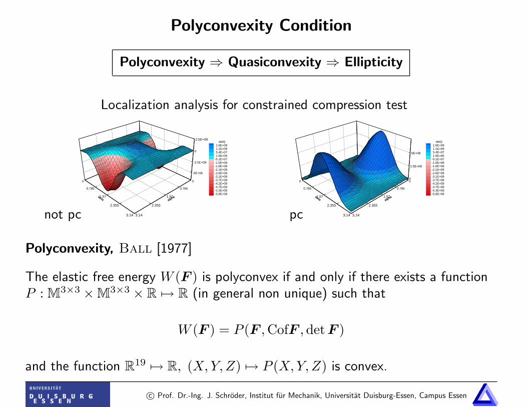
Polyconvexity Condition

Polyconvexity ⇒ Quasiconvexity ⇒ Ellipticity

-5E+08

-2.5E+08

0

2.5E+08

0

0.785

1.57

2.355

3.14

alpha

0

0.785

1.57

2.355

3.14

beta

detQ1.6E+081.1E+085.4E+071.6E+06

-5.1E+07-1.0E+08-1.6E+08-2.1E+08-2.6E+08-3.1E+08-3.7E+08-4.2E+08-4.7E+08-5.3E+08-5.8E+08

not pc

0

2.5E+08

5E+08

0

0.785

1.57

2.355

3.14

alpha

0

0.785

1.57

2.355

3.14

beta

detQ1.6E+081.1E+085.4E+071.6E+06

-5.1E+07-1.0E+08-1.6E+08-2.1E+08-2.6E+08-3.1E+08-3.7E+08-4.2E+08-4.7E+08-5.3E+08-5.8E+08

pc

Localization analysis for constrained compression test

Polyconvexity, Ball [1977]

The elastic free energy W (F ) is polyconvex if and only if there exists a functionP : M3×3 ×M3×3 × R 7→ R (in general non unique) such that

W (F ) = P (F ,CofF ,det F )

and the function R19 7→ R, (X,Y, Z) 7→ P (X,Y, Z) is convex.


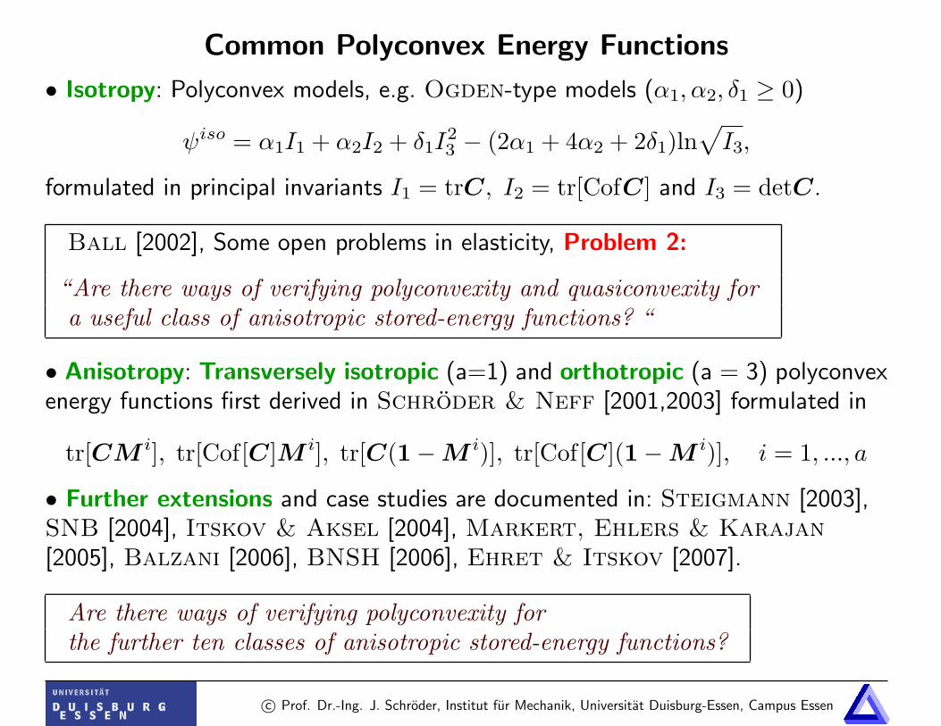
Common Polyconvex Energy Functions

• Isotropy: Polyconvex models, e.g. Ogden-type models (α1, α2, δ1 ≥ 0)

ψiso = α1I1 + α2I2 + δ1I23 − (2α1 + 4α2 + 2δ1)ln

√I3,

formulated in principal invariants I1 = trC, I2 = tr[CofC] and I3 = detC.

Ball [2002], Some open problems in elasticity, Problem 2:

“Are there ways of verifying polyconvexity and quasiconvexity fora useful class of anisotropic stored-energy functions? “

• Anisotropy: Transversely isotropic (a=1) and orthotropic (a = 3) polyconvexenergy functions first derived in Schroder & Neff [2001,2003] formulated in

tr[CM i], tr[Cof[C]M i], tr[C(1−M i)], tr[Cof[C](1−M i)], i = 1, ..., a

• Further extensions and case studies are documented in: Steigmann [2003],SNB [2004], Itskov & Aksel [2004], Markert, Ehlers & Karajan[2005], Balzani [2006], BNSH [2006], Ehret & Itskov [2007].

Are there ways of verifying polyconvexity forthe further ten classes of anisotropic stored-energy functions?


Anisotropic Elasticity

12 anisotropy classes / 32 crystal classes / 7 crystal systems

a1

a3a2

βa2γ

α

a3

a1

with a = ||a1||, b = ||a2||, c = ||a3||

No. crystal system edge lengths axial angle

1 triclinic a 6= b 6= c α 6= β 6= γ 6= 90◦

2 monoclinic a 6= b 6= c α = β = 90◦; γ 6= 90◦

3 trigonal a = b = c α = β = γ 6= 90◦

4 hexagonal a = b 6= c α = β = 90◦; γ = 120◦

5 rhombic a 6= b 6= c α = β = γ = 90◦

6 tetragonal a = b 6= c α = β = γ = 90◦

7 cubic a = b = c α = β = γ = 90◦


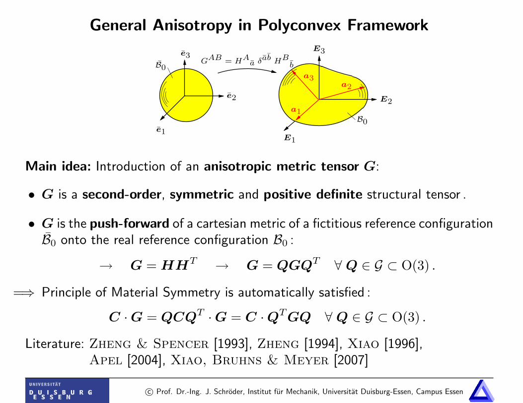
General Anisotropy in Polyconvex Framework

e2

e3

e1

E3

E1

a1

a3a2

B0GAB = HAa δ

ab HBb

E2

B0

Main idea: Introduction of an anisotropic metric tensor G:

• G is a second-order, symmetric and positive definite structural tensor .

• G is the push-forward of a cartesian metric of a fictitious reference configurationB0 onto the real reference configuration B0 :

→ G = HHT → G = QGQT ∀ Q ∈ G ⊂ O(3) .

=⇒ Principle of Material Symmetry is automatically satisfied :

C ·G = QCQT ·G = C ·QTGQ ∀ Q ∈ G ⊂ O(3) .

Literature: Zheng & Spencer [1993], Zheng [1994], Xiao [1996],Apel [2004], Xiao, Bruhns & Meyer [2007]


Metric Tensors for the Seven Crystal Systems

Linear Mapping of the cartesian base vectors onto crystallographic motivated basevectors:

H : ei 7→ ai → H = [a1,a2,a3] with ai = H ei

Special choice: a1 ‖ e1, a2 ⊥ e3 :

a23

a1

γ

α

a22

e3

β

a2

a11a13

a12

a33

e1

e2

a3

H =

a b cos γ c cos β

0 b sin γ c (cosα− cos β cos γ)/ sin γ

0 0 c [1 + 2 cosα cos β cos γ−(cos2 α+ cos2 β + cos2 γ)]1/2/sinγ

E.g. Monoclinic Metric Tensor (a 6= b 6= c, α = β = 90◦, γ 6= 90◦):

Gm = HmHmT =

a2 + b2 cos2 γ b2 cos γ sin γ 0b2 cos γ sin γ b2 sin2 γ 00 0 c2

→ Gm =

a d 0d b 00 0 c


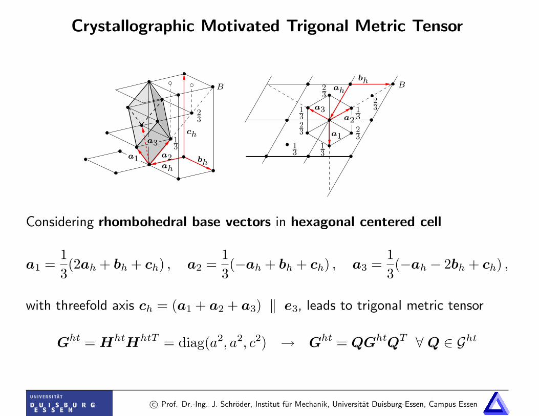
Crystallographic Motivated Trigonal Metric Tensor

232

323

a3

23

bh

13

23

a1

ah

13

bh

B

a2

13

ch

ah

13

B

a1

13a2

a3

Considering rhombohedral base vectors in hexagonal centered cell

a1 =13(2ah + bh + ch) , a2 =

13(−ah + bh + ch) , a3 =

13(−ah − 2bh + ch) ,

with threefold axis ch = (a1 + a2 + a3) ‖ e3, leads to trigonal metric tensor

Ght = HhtHhtT = diag(a2, a2, c2) → Ght = QGhtQT ∀ Q ∈ Ght


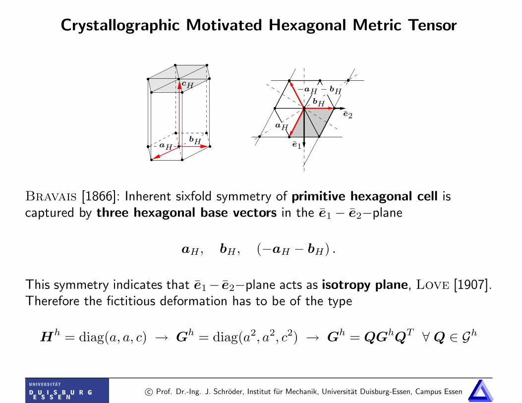
Crystallographic Motivated Hexagonal Metric Tensor

bH

e1

cH

e2

−aH − bH

aH

aHbH

Bravais [1866]: Inherent sixfold symmetry of primitive hexagonal cell iscaptured by three hexagonal base vectors in the e1 − e2−plane

aH, bH, (−aH − bH) .

This symmetry indicates that e1− e2−plane acts as isotropy plane, Love [1907].Therefore the fictitious deformation has to be of the type

Hh = diag(a, a, c) → Gh = diag(a2, a2, c2) → Gh = QGhQT ∀ Q ∈ Gh


Proof of Polyconvexity of tr[CG] and tr[Cof[C]G]

Generic polyconvex anisotropic functions

[tr(F TFG)]k and [tr(Cof(F T )Cof(F )G)]k

with k ≥ 1 and G ∈ Psym.

Proof of Convexity. With identity [tr(F TFG)]k =‖FH ‖2k= 〈FH,FH〉kwe obtain

DF (〈FH,FH〉k) .ξ = 2k〈FH,FH〉k−1〈FH, ξH〉

D2F (〈FH,FH〉k) .(ξ, ξ) = 2k〈FH,FH〉k−1〈ξH, ξH〉

+4k(k − 1)〈FH,FH〉k−2〈FH, ξH〉2

= 2k ‖FH ‖2k−2 ‖ξH ‖2

+4k(k − 1) ‖FH ‖2k−4 〈FH, ξH〉2 ≥ 0.

Detailed proofs are given in Schroder, Neff & Ebbing [2008].


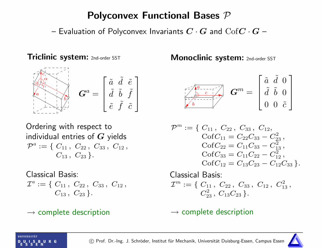
Polyconvex Functional Bases P– Evaluation of Polyconvex Invariants C ·G and CofC ·G –

Triclinic system: 2nd-order SST

ab

αc

β γ

→ complete description

Ga =

a d e

d b f

e f c

Ordering with respect toindividual entries of G yieldsPa := { C11 , C22 , C33 , C12 ,

C13 , C23 }.

Classical Basis:Ia := { C11 , C22 , C33 , C12 ,

C13 , C23 }.

Monoclinic system: 2nd-order SST

b

ca


Gm =

a d 0d b 00 0 c

Pm := { C11 , C22 , C33 , C12,

CofC11 = C22C33 − C223 ,

CofC22 = C11C33 − C213 ,

CofC33 = C11C22 − C212 ,

CofC12 = C13C23 − C12C33 }.

Classical Basis:Im := { C11 , C22 , C33 , C12 , C

213 ,

C223 , C13C23 }.


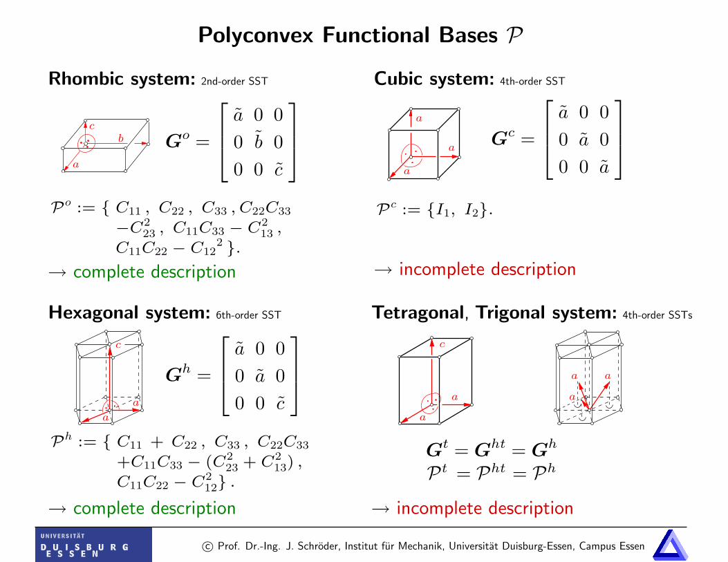
Polyconvex Functional Bases P

Rhombic system: 2nd-order SST

a

bc


Go =

a 0 00 b 00 0 c

Po := { C11 , C22 , C33 , C22C33

−C223 , C11C33 − C2

13 ,

C11C22 − C122 }.

Cubic system: 4th-order SST

a

a

a

→ incomplete description

Gc =

a 0 00 a 00 0 a

Pc := {I1, I2}.

Hexagonal system: 6th-order SST

c

a

a


Gh =

a 0 00 a 00 0 c

Ph := { C11 + C22 , C33 , C22C33

+C11C33 − (C223 + C2

13) ,

C11C22 − C212} .

Tetragonal, Trigonal system: 4th-order SSTs

a

a

c

aa

a

→ incomplete description

Gt = Ght = Gh

Pt = Pht = Ph


Generic Polyconvex Anisotropic Energy Functions

Additive decomposition of the free energy in isotropic and anisotropic terms, i.e.,

ψ = ψiso(I1, I2, I3) + ψaniso(I3, J4j, J5j),

with J4j = tr[CGj] , J5j = tr[Cof[C]Gj] and the j-th metric tensor Gj.

For the isotropic part ψiso we choose a compressible Mooney-Rivlin model,i.e.,

ψiso = α1 I1 + α2 I2 + δ1 I3 − δ2ln(√I3), ∀ α1, α2, δ1, δ2 ≥ 0.

Suitable polyconvex anisotropic energies in terms of f3rj, f4rj, f5rj, f6rj, f7rj

ψaniso1 =n∑r=1

m∑j=1

[f3rj(I3) + f4rj(J4j) + f5rj(J5j)] ,

ψaniso2 =n∑r=1

m∑j=1

[f3rj(I3) + f6rj(I3, J4j) + f7rj(I3, J5j)] ,

ψaniso3 =n∑r=1

m∑j=1

[f3rj(I3) + f4rj(J4j) + f5rj(J5j)

+f6rj(I3, J4j) + f7rj(I3, J5j)] .

Further details: Schroder, Neff & Ebbing [2008].


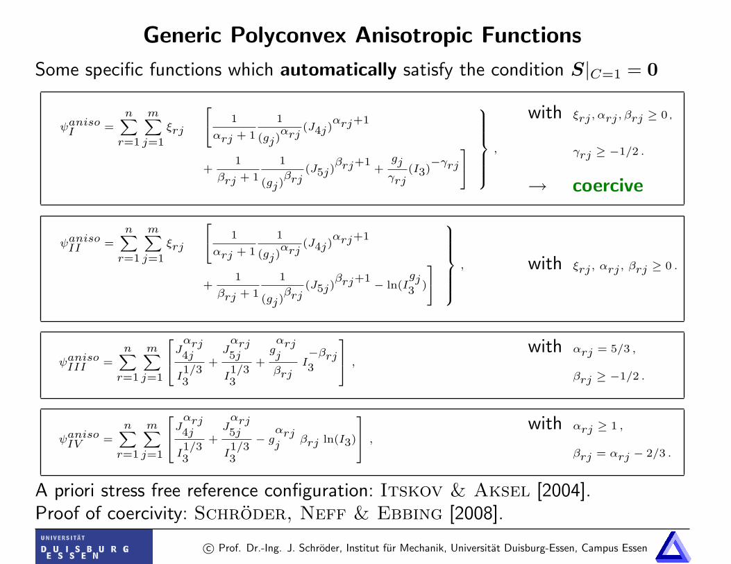
Generic Polyconvex Anisotropic Functions

Some specific functions which automatically satisfy the condition S|C=1 = 0

ψanisoI =nXr=1

mXj=1

ξrj

24 1

αrj + 1

1

(gj)αrj

(J4j)αrj+1

+1

βrj + 1

1

(gj)βrj

(J5j)βrj+1

+gj

γrj(I3)

−γrj35

9>>>>>>=>>>>>>;,

with ξrj, αrj, βrj ≥ 0 ,

γrj ≥ −1/2 .

→ coercive

ψanisoII =nXr=1

mXj=1

ξrj

24 1

αrj + 1

1

(gj)αrj

(J4j)αrj+1

+1

βrj + 1

1

(gj)βrj

(J5j)βrj+1 − ln(I

gj3 )

35

9>>>>>>=>>>>>>;, with ξrj, αrj, βrj ≥ 0 .

ψanisoIII =nXr=1

mXj=1

264Jαrj4j

I1/33

+Jαrj5j

I1/33

+gαrjj

βrjI−βrj3

375 ,with αrj = 5/3 ,

βrj ≥ −1/2 .

ψanisoIV =nXr=1

mXj=1

264Jαrj4j

I1/33

+Jαrj5j

I1/33

− gαrjj

βrj ln(I3)

375 ,with αrj ≥ 1 ,

βrj = αrj − 2/3 .

A priori stress free reference configuration: Itskov & Aksel [2004].Proof of coercivity: Schroder, Neff & Ebbing [2008].


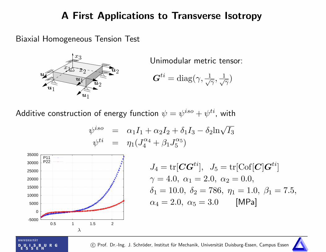
A First Applications to Transverse Isotropy

Biaxial Homogeneous Tension Test

x1

u1u1

x2

x3

u1 u1

u2

u2

Unimodular metric tensor:

Gti = diag(γ, 1√γ ,

1√γ)

Additive construction of energy function ψ = ψiso + ψti, with

ψiso = α1I1 + α2I2 + δ1I3 − δ2ln√I3

ψti = η1(Jα44 + β1J

α55 )

-5000

0

5000

10000

15000

20000

25000

30000

35000

0.5 1 1.5 2

P11P22

λ

J4 = tr[CGti], J5 = tr[Cof[C]Gti]γ = 4.0, α1 = 2.0, α2 = 0.0,δ1 = 10.0, δ2 = 786, η1 = 1.0, β1 = 7.5,α4 = 2.0, α5 = 3.0 [MPa]


Fitting of Monoclinic Moduli C = 4∂2CCψ: Augite

movie

movie

Characteristic surfaces

Young’s modulus

Bulk modulus

Elasticities in [GPa], Simmons [1971]:

C(V )exp =

217.8 72.4 33.9 24.6 0 0

181.6 73.4 19.9 0 0150.7 16.6 0 0

51.1 0 0sym. 55.8 4.3

69.7

Error for ψ = ψanisoI and n = m = 3 :

e =‖ C(V )comp − C(V )exp ‖

‖ C(V )exp ‖≈ 3.48[%]

Metric Tensors:

Gti1 = diag(0.419, 0.419, 1.953),

Gm2 =

[1.503 −0.513 0

−0.513 0.934 0

0 0 1.572

], Gm

3 =

[2.719 0.496 0

0.496 0.547 0

0 0 1.008

]


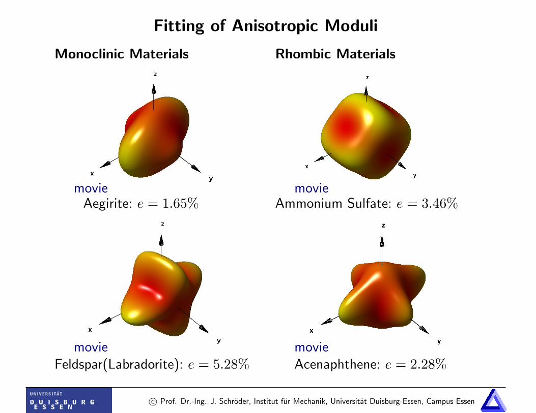
Fitting of Anisotropic Moduli

movieAegirite: e = 1.65%

movieFeldspar(Labradorite): e = 5.28%

movieAmmonium Sulfate: e = 3.46%

movieAcenaphthene: e = 2.28%

Monoclinic Materials Rhombic Materials


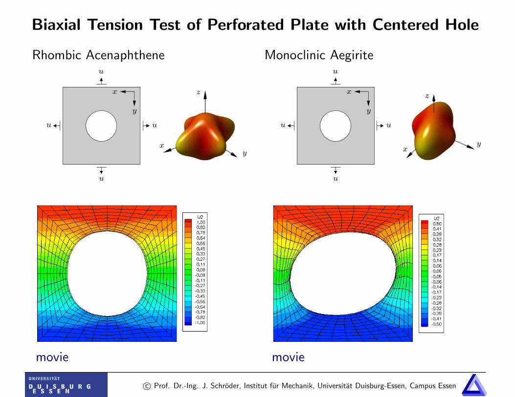
Biaxial Tension Test of Perforated Plate with Centered Hole

movie movie

u

u

u

u

x

y

u

u

u

u

x

y

Rhombic Acenaphthene Monoclinic Aegirite

xy

z

xy

z


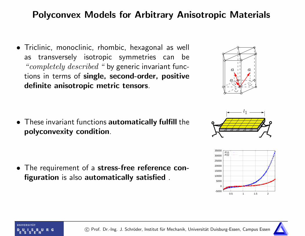
Polyconvex Models for Arbitrary Anisotropic Materials

• Triclinic, monoclinic, rhombic, hexagonal as wellas transversely isotropic symmetries can be“completely described “ by generic invariant func-tions in terms of single, second-order, positivedefinite anisotropic metric tensors.

aa

a

• These invariant functions automatically fulfill thepolyconvexity condition.

l1

• The requirement of a stress-free reference con-figuration is also automatically satisfied .

-5000

0

5000

10000

15000

20000

25000

30000

35000

0.5 1 1.5 2

P11P22


Selected References

- Balzani, D.; Neff, P.; Schroder, J. & Holzapfel, G.A. [2006],“A polyconvex framework for soft biological tissues. Adjustment to experimentaldata”, IJSS, Vol. 43, No. 20, 6052–6070

- Ebbing, V.; Schroder, J. & Neff, P. [2007], “On the construction ofanisotropic polyconvex energy densities”, PAMM, Vol. 7

- Hartmann, S. & Neff, P. [2003], “Polyconvexity of generalized polynomialtype hyperelastic strain energy functions for near incompressibility”, IJSS, Vol.40, 2767–2791

- Schroder, J. & Neff, P. [2001], “On the construction of polyconvex ani-sotropic free energy functions”, in Proceedings of the IUTAM Symposium onComputational Mechanics of Solid Materials at Large Strains, 171–180

- Schroder, J. & Neff, P. [2003], “Invariant formulation of hyperelastictransverse isotropy based on polyconvex free energy functions”, IJSS, Vol. 40,401–445

- Schroder, J.; Neff, P. & Balzani, D. [2004], “A variational approach formaterially stable anisotropic hyperelasticity”, IJSS, Vol. 42/15, 4352–4371

- Schroder, J.; Neff, P. & Ebbing, V. [2008], “Anisotropic PolyconvexEnergies on the Basis of Crystallographic Motivated Structural Tensors”, sub-mitted to JMPS


polyconvex models for arbitrary anisotropic materials l1

Documents