Pollard’s p-1 and Lenstra’s factoringalgorithms

Anne-Sophie Charest

October 2, 2005

Abstract

This paper presents the result of my summer research on Lenstra’salgorithm for factoring with elliptic curves. It first describes Pollard’sp-1 algorithm, which is in a way the basis for Lenstra’s algorithm. Thetheory behind both algorithms will be discussed, as well as the theirdetailed steps, their implementation and their efficiency. This paperis intended for people with little previous knowledge in group theory.Understanding of basic algebra, such as the ideas of gcd and modulararithmetic, is assumed.

Contents

1 Pollard’s p-1 algorithm 31.1 General idea of the algorithm . . . . . . . . . . . . . . . . . . 31.2 The steps of the algorithm . . . . . . . . . . . . . . . . . . . . 41.3 Conditions of success of the algorithm . . . . . . . . . . . . . . 51.4 Efficiency of the algorithm . . . . . . . . . . . . . . . . . . . . 51.5 Possible improvements of the algorithm . . . . . . . . . . . . . 10

2 Lenstra’s algorithm using elliptic curves 112.1 Elliptic curves . . . . . . . . . . . . . . . . . . . . . . . . . . . 112.2 General idea of the algorithm . . . . . . . . . . . . . . . . . . 142.3 The steps of the algorithm . . . . . . . . . . . . . . . . . . . . 152.4 Conditions of success of the algorithm . . . . . . . . . . . . . . 152.5 Efficiency of the algorithm . . . . . . . . . . . . . . . . . . . . 162.6 Possible improvements of the algorithm . . . . . . . . . . . . . 19

1

Introduction

Number theory, although once renowned and loved for its lack of applicationto the real world, is now used in many ways in our everyday life. It’s thebasis of the the RSA cryptography system [8], used by millions of people ev-eryday to exchange secret information, such as credit card numbers, over theInternet. This cryptosystem relies on the fact that it is much more easier totest for primality than to factor integers, which means that we can find twobig primes and multiply them together without too much trouble, but we cannot compute the unique factorisation into primes of the resulting compositein a reasonable amount of time. (For more detailed information on how theRSA cryptographic system and general concepts of cryptography, see [12].)However, the difficulty of factoring integers has not yet been proven, andthis entire system would collapse if it were false and an efficient factoringalgorithm were invented. This is what motivates in great part the search forfast factoring.

The idea of factoring an integer into primes is a very simple one. It canbe performed properly by any elementary school student by dividing the in-teger to factor succesively by all integers smaller than its squareroot. Thistechnique is straigthforward and always successful, but requires many oper-ations. Inded, to find one factor of an integer n we might have to try up to√

n possible divisors. Thus, when the numbers to factorize get huge, such asin the cryptographic setting, this technique becomes rapidly unsuable. Tothis date, no computer is fast enough to factor large integers of about 300digits in fewer than millions of years [3]. Hence, even if the speed of our com-puters would increase drastically, we would still rapidly run into numbers wecouldn’t factor in less than thousands of years.

So, the search for faster factorisation is really the search for new algo-rithms that factor integers in less operations. This report will present twoalgorithms that I have studied over the summer : Pollard’s p-1 algorithmand Lenstra’s algorithm using elliptic curves, the first one being the basis ofthe other one. Although they are not the fastest current algorithms to factorany integer, they can yield impressive results for factoring some particularkind of integers.

2

1 Pollard’s p-1 algorithm

1.1 General idea of the algorithm

The p − 1 algorithm was developped by J.M.Pollard in the 1970’s [6] . Thebasic idea of the algorithm is to use some information about the order of anelement of the group Zp to find a factor p of N . The algorithm is based onthe following theorem :

Theorem 1.1. Fermat’s Little TheoremLet p be a prime and a ε Z such that p - a . Then, ap−1 ≡ 1 mod p.

Proof. Consider the following two sets of equivalence classes :

A = {[a], [2a], [3a], [4a], . . . , [(p− 1)a]}

B = {[1], [2], [3], [4], . . . , [p− 1]} = Zp − {[0]}

First, we want to show that A = B.Clearly, A ⊆ B since p - a and p divides none of 1, 2, 3, . . . , p− 1.Now, suppose that ∃ r, s εN such that 1 ≤ r ≤ s ≤ p− 1 and [ra] = [sa].Then,

[ra]− [sa] = 0

r[a]− s[a] = 0

(r − s)[a] = 0

r − s = 0, since[a] 6= 0 mod p (since p - a)

But, since r ≤ p and s ≤ p, r − s ≡ 0 mod p ⇒ r = s.So, [a], [2a], [3a], · · · , [(p− 1)a] are all different mod p, which means that thecardinality of A is p− 1.And, since ]A = p− 1, ]B = p− 1 and A ⊆ B, we can conclude that A = B,that is the equivalence classes in A are congruent to the equivalence classesof B under a certain rearrangement.Hence,

a ∗ 2a ∗ 3a ∗ · · · ∗ (p− 1)a = 1 ∗ 2 ∗ 3 ∗ · · · ∗ p− 1 mod p

ap−1 ∗ (p− 1)! = (p− 1)!

ap−1 = 1, since(p− 1)! 6= 0 mod p.

3

Note that from a group theory point of view, considering all a ε Z suchthat p - a as Zp, this theorem is equivalent to the theorem that any elementof a group elevated to the cardinality of the group must equal the identityelement.

How can we use this theorem to factor an integer n ? The idea is thatif p | n, and p is prime, then ap−1 = 1 mod p, or d = ap−1 − 1 = 0 mod p,for any a relatively prime to p, so that gcd(d, n) = p, the factor of n we werelooking for. Obviously, we can not directly compute d because we do notknow p at first. We could just compute am with an exponent m = 1, 2, 3, . . .until gcd(d, n) = p, that is until m = p − 1. However, that would not bemore efficient than doing trial division, since we would need to execute p− 1operations, each involving exponentiaton to a relatively big power.There is however a clever way to choose m. The idea is to notice that wedo not need to exponentiate a exactly to the power m = p− 1 since, if m issuch that p− 1 | m, i.e. m = c(p− 1), then

am − 1 = ac(p−1) − 1 = ap−1c − 1 = 1c ≡ 0 mod p

so that gcd(am, n) = p. So, we need to choose an integer m and we will geta factor of n if p− 1 | m. By choosing m as a product of many small primefactors, the chances that this condition holds will increase.

1.2 The steps of the algorithm

1- Choose a bound B for the algorithm, usually about 105 − 106

2- Compute

m =∏

p prime1≤p≤B

pblogB/logpc

3- Choose a random positive integer a between 1 and n.

4- Compute d = gcd(a, n).If d = 1,go to 5.If d 6= 1, return d. (It is a non-trivial factor of n.)

5- Compute am mod n

6- Compute e = gcd(am − 1, n)If e = 1, go to 1 and increase B.If e = n, go to 3 and change a.If e 6= 1 & e 6= n, return d. (It is a non-trivial factor of n.)

4

Note that the bound B defines indirectly the size of the exponent m. Ithence constitutes a measure of the time the algorithm will take to factorn. A bigger B increases the probability of finding a factor of n, but it alsoincreases the time needed to perform the algorithm.

I should also point out that some implementations of the algorithm willuse m = lcm(B). Then, m will still be a product of small primes, but itsfactorisation will not include any power of small primes, so it might fail ifthe factorization of p− 1 contains a prime to a higher power.

1.3 Conditions of success of the algorithm

Pollard’s algorithm will succeed to find a factor p of n if p is such thatp − 1 | m. Using the following definition of an x-smooth integer, we canrestate this condition as follow : Pollard’s p− 1 algorithm with bound b willsucceed to find a factor of n if n has a factor p such that p− 1 is b-smooth,except in the rare cases where p− 1 has a small prime factor to an exponentso large that it is not in the factorisation of m.

Definition 1.1. An integer n is said to be x-smooth if and only if all itsprime factors are smaller or equal to x.

For example, 153 = 32 ∗ 17 is 17-smooth (and so n-smooth ∀nεN ≥ 17).

Obviously, since n, the number to factorize, is finite, p is finite too, sothere surely exists a B such that p− 1 is b-smooth. However, if this B is toobig, then Pollard’s p − 1 algorithm will not be faster than trial division. Ifwe use Pollard’s p-1 algoithm with a bound B to try to factor n, and n hasa prime factor p, then the probability that we will find p is the probabilitythat p is B − smooth. This probability is approximated by the probabilitythat a number near p is B − smooth,which is given by p((log(p))(log(B)) (Theorem 4.9 of [12]).

1.4 Efficiency of the algorithm

There are three possibly time-consumming steps in the Pollard’s p− 1 algo-rithm:

1- Compute m = lcm(b)

2- Compute am mod n

3- Compute d = gcd(am − 1, n)

In this section, I will present some simple algorithms to do each of theseoperations efficiently.

5

Compute m = lcm(b) : Sieve of Eratosthenes

To compute m, we first need to generate a list of all the primes leqB.One technique to find all those primes would be to go through all the in-tegers smaller than B and check if they are primes. Using trial divison tocheck primality, this technique would require O(

√(i)) steps for each integer

2 ≤ i ≤ B, for a total of O(B√

(B)) steps. This is way too much work foronly a preliminary computation.

Finding those primes can be achieved in a faster way by the Sieve of Er-atosthenes. First, we write all the integers between 2 and our bound B.Then, for each number up to

√(B) which is not crossed out yet, we cross

out all its multiples. The numbers remaining will be the integers smallerthan B which have no factor smaller than

√(B), that is the primes smaller

than B. See annex 1 for a sample code of the Sieve of Eratosthenes in Parilanguage.

The Sieve of Eratosthenes is very more efficient than the trivial method.The outer loop will go through all numbers smaller than

√(B) not yet crossed

out. The exact number that is is not really important, we will just bound itabove by

√(B). For each of these integers, we will cross out at most n

p terms. So, the total needed operations will be :

Σ

√(B)

p=2 dBpe ≈

∫ √(B)

2

B

pdp = B · ln(

√(B)) = O(B · log(B))

Moreover, it is faster to add integers and croos-out numbers than to prodeedto divisions, so the advantage of the Sieve of Erasthostenes over the trialdivision method is even greater than shown by this complexity analysis. Asan indication of how long it takes to compute the primes, the implementationfound in annex returns all the primes smaller than 500 000 in less than onesecond on an average computer.

Compute am mod n : Fast modular multiplication

We will compute am mod n by expending m as a sum of powers of 2, repet-edly squaring a, and then multiplying the relevent powers of a.

Let m = k020 + k12

1 + ·+ kr2r, where the ki′s are either 0 or 1.

6

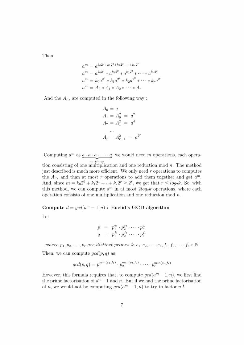
Then,

am = ak020+k122+k222+···+kr2r

am = ak020 ∗ ak122 ∗ ak222 ∗ · · · ∗ akr2r

am = k0a20 ∗ k1a

22 ∗ k2a22 ∗ · · · ∗ kra

2r

am = A0 ∗ A1 ∗ A2 ∗ · · · ∗ Ar

And the Ai′s are computed in the following way :

A0 = a

A1 = A20 = a2

A2 = A21 = a4

...

Ar = A2r−1 = a2r

Computing am as a · a · a · · · · · a︸ ︷︷ ︸m times

, we would need m operations, each opera-

tion consisting of one multiplication and one reduction mod n. The methodjust described is much more efficient. We only need r operations to computesthe Ai′s and than at most r operations to add them together and get am.And, since m = k02

0 + k121 + ·+ kr2

r ≥ 2r, we get that r ≤ log2k. So, withthis method, we can compute am in at most 2log2k operations, where eachoperation consists of one multiplication and one reduction mod n.

Compute d = gcd(am − 1, n) : Euclid’s GCD algorithm

Let

p = pe11 · pe2

2 · · · · · perr

q = pf1

1 · pf2

2 · · · · · pfrr

where p1, p2, . . . , pr are distinct primes & e1, e2, . . . , er, f1, f2, . . . , fr ε N

Then, we can compute gcd(p, q) as

gcd(p, q) = pmin(e1,f1)1 · pmin(e2,f2)

2 · · · · · pmin(er,fr)r

However, this formula requires that, to compute gcd(am − 1, n), we first findthe prime factorisation of am−1 and n. But if we had the prime factorisationof n, we would not be computing gcd(am − 1, n) to try to factor n !

7

The problem of computing the gcd of two integers whose factorisationinto primes we do not know has fortunately been successfully studied longago. Indeed, Euclid published a method to find gcd(p, q) as Proposition II inthe second book of The Elements more than 2000 years ago. It is based onthe following theorem :

Theorem 1.2. GCD and remainderLet a, b ε N+ and q, r εZ such that a = bq + r. Then, gcd(a, b) = gcd(r, b).

Proof. Let d = gcd(a, b) and e = gcd(r, b).We will show that d ≤ e and e ≤ d, so that d = e.

d | a & d | b ⇒ d | a− bq = r

So, d is a common divisor of b and r. And, since e = gcd(b, r), d ≤ e.Also,

e | r & e | b ⇒ e | bq − r = a

So, e is a common divisor of a and b. And, since d = gcd(a, b), e ≤ d.Hence, d = e, i.e gcd(a, b) = gcd(b, r).

Euclid’s algorithm consists of reducing the problem of computing gcd(a, b)of size a to the problem of computing gcd(b, r = a−qb) of size b by the divisionalgorithm and then applying the same technique until we get the gcd(a, b) :

a = bq1 + r1 0 ≤ r1 < b

b = r1q2 + r2 0 ≤ r2 < r1

...

rn−1 = rnqn+1 + rn+1 0 ≤ rn+1 < rn

rn = rn+1qn+2

Since the sequence of remainders is strictly decreasing and the remaindersare all strictly positive, there will necessarily eventually be one remainderequal to 0. In our example, it was rn+2, and so

gcd(a, b) = gcd(b, r1) = . . . = gcd(rn, rn+1) = rn+1

Euclid’s algorithm is really simple to implement recursively. Here is my codeof the Euclidean algorithm in Pari :

8

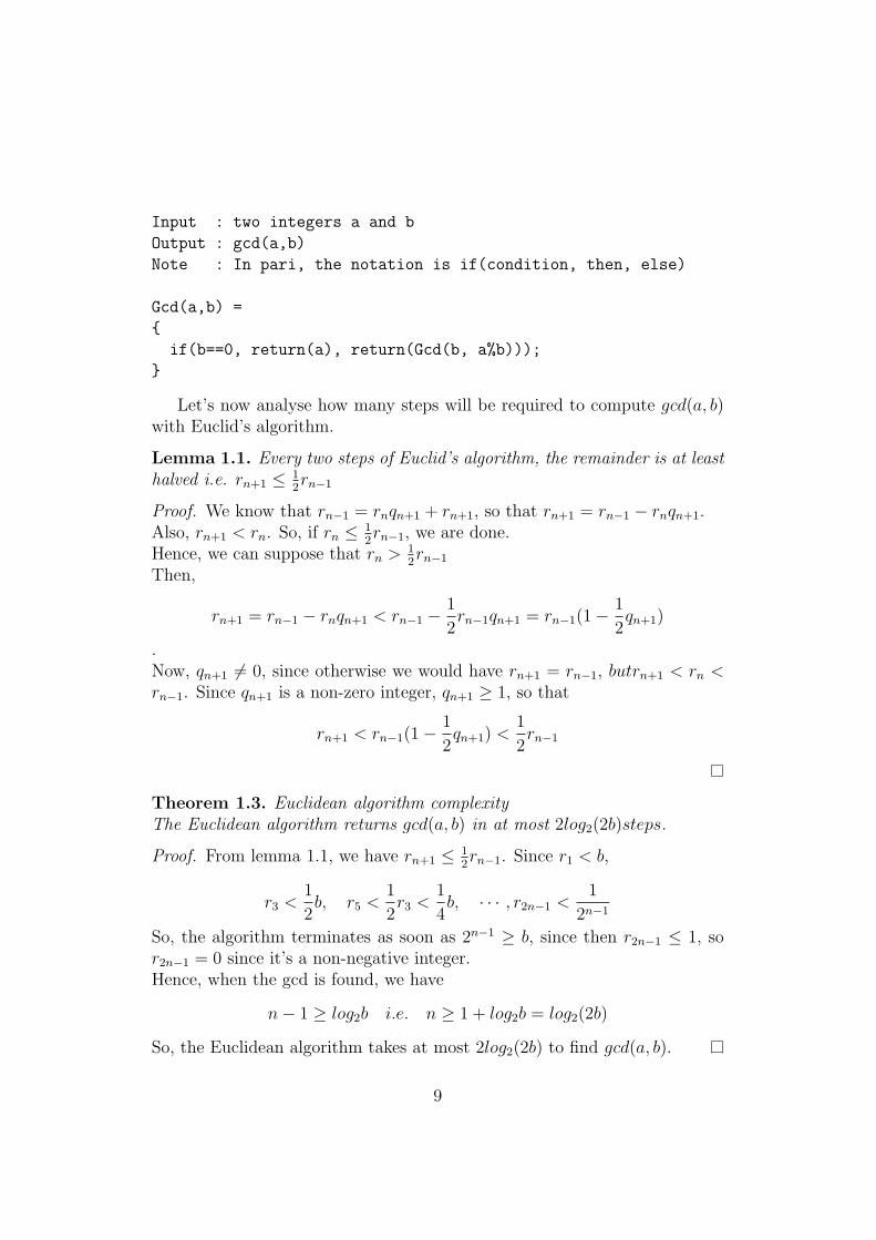
Input : two integers a and b

Output : gcd(a,b)

Note : In pari, the notation is if(condition, then, else)

Gcd(a,b) =

{

if(b==0, return(a), return(Gcd(b, a%b)));

}

Let’s now analyse how many steps will be required to compute gcd(a, b)with Euclid’s algorithm.

Lemma 1.1. Every two steps of Euclid’s algorithm, the remainder is at leasthalved i.e. rn+1 ≤ 1

2rn−1

Proof. We know that rn−1 = rnqn+1 + rn+1, so that rn+1 = rn−1 − rnqn+1.Also, rn+1 < rn. So, if rn ≤ 1

2rn−1, we are done.

Hence, we can suppose that rn > 12rn−1

Then,

rn+1 = rn−1 − rnqn+1 < rn−1 −1

2rn−1qn+1 = rn−1(1−

1

2qn+1)

.Now, qn+1 6= 0, since otherwise we would have rn+1 = rn−1, butrn+1 < rn <rn−1. Since qn+1 is a non-zero integer, qn+1 ≥ 1, so that

rn+1 < rn−1(1−1

2qn+1) <

1

2rn−1

Theorem 1.3. Euclidean algorithm complexityThe Euclidean algorithm returns gcd(a, b) in at most 2log2(2b)steps.

Proof. From lemma 1.1, we have rn+1 ≤ 12rn−1. Since r1 < b,

r3 <1

2b, r5 <

1

2r3 <

1

4b, · · · , r2n−1 <

1

2n−1

So, the algorithm terminates as soon as 2n−1 ≥ b, since then r2n−1 ≤ 1, sor2n−1 = 0 since it’s a non-negative integer.Hence, when the gcd is found, we have

n− 1 ≥ log2b i.e. n ≥ 1 + log2b = log2(2b)

So, the Euclidean algorithm takes at most 2log2(2b) to find gcd(a, b).

9

1.5 Possible improvements of the algorithm

When the bound B becomes so big that it is too expensive to continue doingPollard’s algorithm as describe earlier, there is still a possibility to go on andfactor n, which is a second-stage to the algorithm. At this point, we changethe notation of B to B1, and introduce a new bound B2, usually 100B1 or10000B1. (This actually depends of our implementation, but to increase ourchances of finding a factor, it is suggested in [7] to choose B2 such that ouralgorithm will spend as much time in the second phase as it spend in thefirst one.)

So, in the second stage, we keep the value aQ, where Q = lcm(primes ≤ B1)and we then compute aQq1 , aQq2 , · · · , aQqr , where q1, q2, · · · , qr are all theprimes between B1 and B2, and check each time gcd(aQqi − 1, n) just as inthe last step of the first stage. To compute aQqs from aQqr , compute aQ(qs−qr).Since the difference between two primes is usually not too big, this is doneefficiently by precomputing a2Q, a4Q, · · · , aQ2n with n being a few hundredsbefore starting stage 2.

The second stage of Pollard’s algorithm will find a factor p if its p− 1 primefactors are all ≤ B1 except for one which is between B1 and B2. Notice thatit will not find a factor p if p−1 as more than one factor between B1 and B2because the prime factors are included only one at a time in the exponent,except in a few particuliar cases.

Some other technical improvement can also make the algorithm run faster.For example, we could compute the gcd’s only once a few hundred times,and then go backwards if more than one factor has been found. Some detailson other speeding improvements can be found in [5]. However, even with allthese improvements, Pollard’s algorithm will not factor n if p−1 only has bigprimes in its factorization. At this point, it is better to switch to an otheralgorithm, for example Lenstra’s factoring method which extends the idea ofthe p− 1 algorithm to the group of points on an elliptic curve.

10

2 Lenstra’s algorithm using elliptic curves

Before we study Lenstra’s algorithm for factoring integers with elliptic curves,we need to take a look at a few properties of elliptic curves.

2.1 Elliptic curves

Definition

An elliptic curve is defined by a polynomial of degree threee of two variables,f(x, y) = 0, where x and y are taken from an arbitrary field. By an appro-priate change of variables, any elliptic curve can be reduced to the followingWeierstrass form : y2 = x3 +ax+ b, provided the field over which the ellipticcurve is defined does not have characteristic 2 or 3. We have to exclude thesecases because transforming a general elliptic curve into the Weierstrass forminvolves division by 2 and by 3, which then would not be allowed. Since thealgorithm does not require any elliptic curve over a field of characteristic 2 or3, we will not consider them, and concentratre only on elliptic curves in theWeierstrass form, as this simplifies considerably our work. So, our definitionof an elliptic curve is as follow :

Definition 2.1. An elliptic curve is defined by a non-singular equation of theform y2 = x3 +ax+b where a, b, x, y ε K, and K is a field with characteristic6= 2, 3.

Non-singularity of the curve only means that it does not have any repeatedroots, that is its graph does not have any cusps or self-intersections. Justas the discriminant b2 − 4ac of a quadratic equation ax2 + bx + c vanishesif the equation has a repeated root, the discriminant ∆ = −16(4a3 + 27b2)of an elliptic curve will vanish if the curve is non-singular. So, we check fornon-singularity by adding the condition that 4a3 + 27b 6= 0.

One interesting geometric property of a curve as defined in 2.1 is that anyline crossing the curve at two points on the plane will necessarily meet it ata third point. To see that, suppose that the line is given by y = mx + b andlook at its intersections with the curve y2 = x3 + ax + b. The points whichare both on the line and the curve will satisfy the equation

y2 = (mx + b)2 = mx2 + 2bm + b2 = x3 + ax + b

And,this is a cubic equation in x, so it has either 3 real roots or only 1.

11

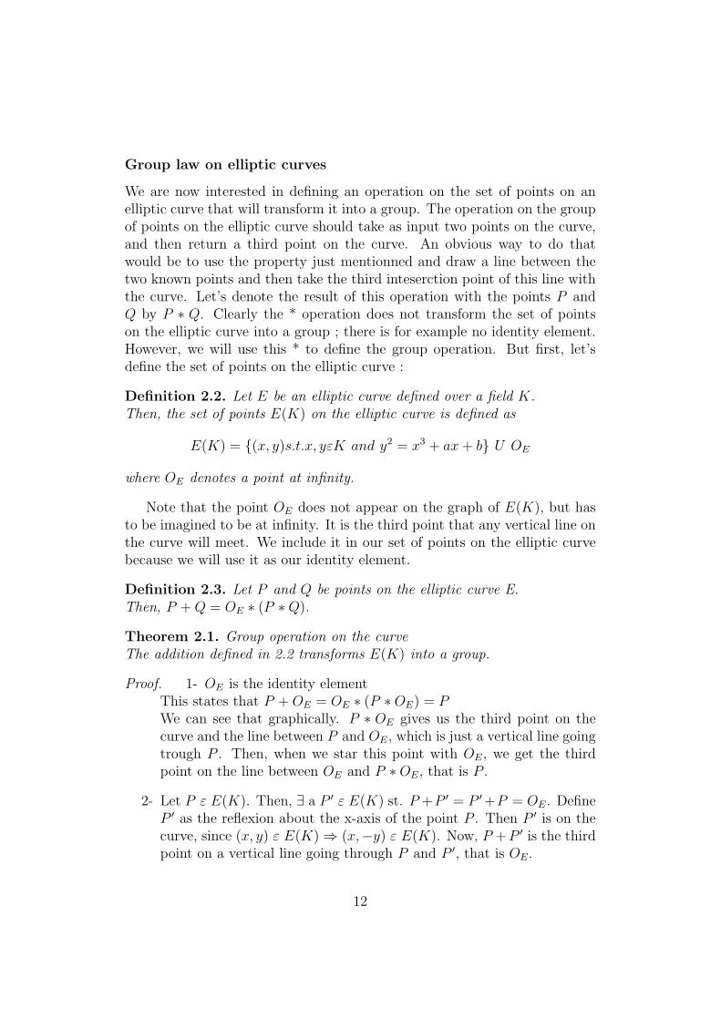
Group law on elliptic curves

We are now interested in defining an operation on the set of points on anelliptic curve that will transform it into a group. The operation on the groupof points on the elliptic curve should take as input two points on the curve,and then return a third point on the curve. An obvious way to do thatwould be to use the property just mentionned and draw a line between thetwo known points and then take the third inteserction point of this line withthe curve. Let’s denote the result of this operation with the points P andQ by P ∗ Q. Clearly the * operation does not transform the set of pointson the elliptic curve into a group ; there is for example no identity element.However, we will use this * to define the group operation. But first, let’sdefine the set of points on the elliptic curve :

Definition 2.2. Let E be an elliptic curve defined over a field K.Then, the set of points E(K) on the elliptic curve is defined as

E(K) = {(x, y)s.t.x, yεK and y2 = x3 + ax + b} U OE

where OE denotes a point at infinity.

Note that the point OE does not appear on the graph of E(K), but hasto be imagined to be at infinity. It is the third point that any vertical line onthe curve will meet. We include it in our set of points on the elliptic curvebecause we will use it as our identity element.

Definition 2.3. Let P and Q be points on the elliptic curve E.Then, P + Q = OE ∗ (P ∗Q).

Theorem 2.1. Group operation on the curveThe addition defined in 2.2 transforms E(K) into a group.

Proof. 1- OE is the identity elementThis states that P + OE = OE ∗ (P ∗OE) = PWe can see that graphically. P ∗ OE gives us the third point on thecurve and the line between P and OE, which is just a vertical line goingtrough P . Then, when we star this point with OE, we get the thirdpoint on the line between OE and P ∗OE, that is P .

2- Let P ε E(K). Then, ∃ a P ′ ε E(K) st. P +P ′ = P ′+P = OE. DefineP ′ as the reflexion about the x-axis of the point P . Then P ′ is on thecurve, since (x, y) ε E(K) ⇒ (x,−y) ε E(K). Now, P +P ′ is the thirdpoint on a vertical line going through P and P ′, that is OE.

12

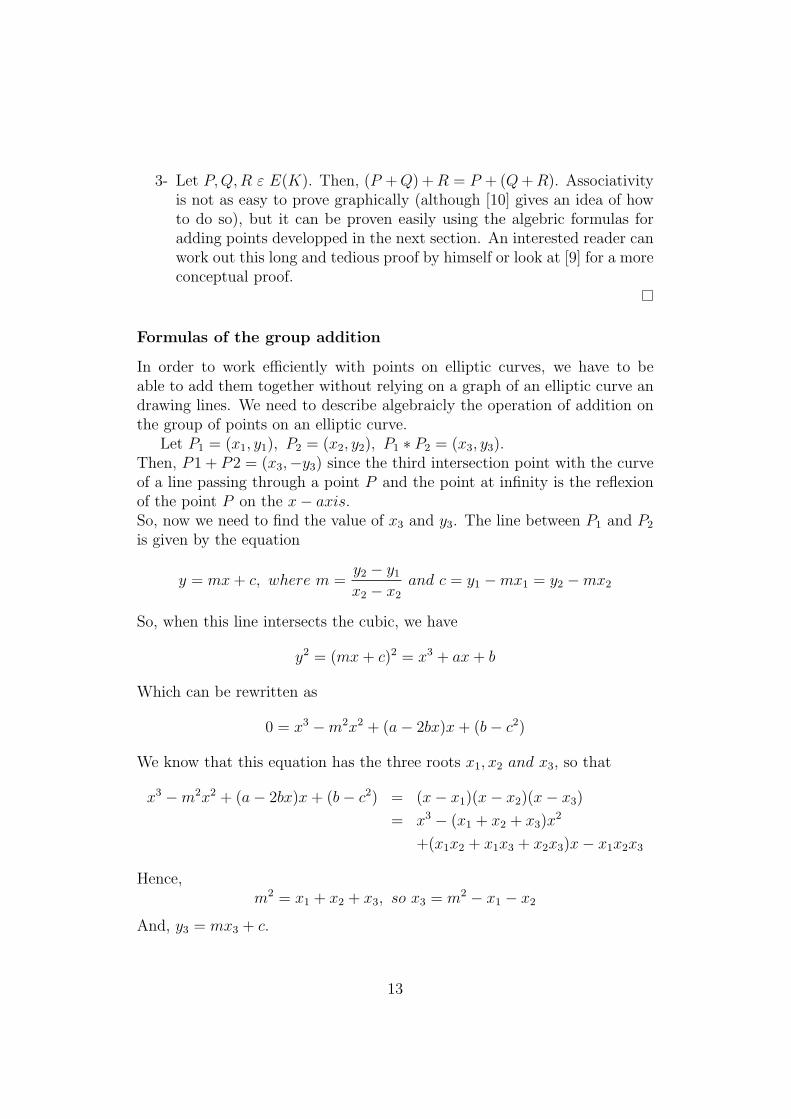
3- Let P, Q,R ε E(K). Then, (P + Q) + R = P + (Q + R). Associativityis not as easy to prove graphically (although [10] gives an idea of howto do so), but it can be proven easily using the algebric formulas foradding points developped in the next section. An interested reader canwork out this long and tedious proof by himself or look at [9] for a moreconceptual proof.

Formulas of the group addition

In order to work efficiently with points on elliptic curves, we have to beable to add them together without relying on a graph of an elliptic curve andrawing lines. We need to describe algebraicly the operation of addition onthe group of points on an elliptic curve.

Let P1 = (x1, y1), P2 = (x2, y2), P1 ∗ P2 = (x3, y3).Then, P1 + P2 = (x3,−y3) since the third intersection point with the curveof a line passing through a point P and the point at infinity is the reflexionof the point P on the x− axis.So, now we need to find the value of x3 and y3. The line between P1 and P2

is given by the equation

y = mx + c, where m =y2 − y1

x2 − x2

and c = y1 −mx1 = y2 −mx2

So, when this line intersects the cubic, we have

y2 = (mx + c)2 = x3 + ax + b

Which can be rewritten as

0 = x3 −m2x2 + (a− 2bx)x + (b− c2)

We know that this equation has the three roots x1, x2 and x3, so that

x3 −m2x2 + (a− 2bx)x + (b− c2) = (x− x1)(x− x2)(x− x3)

= x3 − (x1 + x2 + x3)x2

+(x1x2 + x1x3 + x2x3)x− x1x2x3

Hence,m2 = x1 + x2 + x3, so x3 = m2 − x1 − x2

And, y3 = mx3 + c.

13

But, in the case where P1 = P2, we can not use these equations sincecomputing m will involve a division by zero. In this case, we find the slopem by computing the tangent of the curve at the point P1 = P2:

y2 = f(x) = x3 + ax + b

So, m =dy

dx=

f ′(x)

2y=

3x2 + a

2y

Hence, we can add two points P1 = (x1, y1) and P2 = (x2, y2) on theelliptic curve y2 = x3 + ax + b in the following way :

P1 + P2 =

{OE if P1 = −P2

(m2 − x1 − x2, m(x1 − x3)− y1) otherwise

where

m =

{3x2

1+a

2y1if P1 = P2

y2−y1

x2−x1otherwise

2.2 General idea of the algorithm

Recall that in Pollard’s p-1 algorithm, we can not factor n if it doesn’t havea prime factor p with p − 1 smooth. H.W. Lenstra developped in 1985 [4]a new factorisation algorithm which avoid this problem b use the group ofrandom elliptic curve over the field Zp instead than the multiplicative groupof Zp. The idea is that the later always has order p− 1, but the order of thegroup on an elliptic curve varies with the curve, so that if the order is notsmooth enough, we can just change curve.

Since we do not know p at first, we can not define an elliptic curve overthe field Zp. So, we define the elliptic curve over the ring Zn. Technically anelliptic curve modulo n is not really an elliptic curve. But, by the Chineseremainder theorem, what goes on modn can be imagined seperatly modp andmodq for factors p and q of n. By adding the condition that for the ellipticcurve gcd(4a3 + 27b2, n) = 1, we ensure that it is actually an elliptic curvemod p and modq.

Now, we want to find a number k which is congruent to 0 mod p ormod q, but only for one at a time, so that gcd(k, n) is a non-trivial factorof n. To find this number,we add a point with himself a certain number oftimes using the formulas derived earlier. We can do that even if we do not

14

work over a ring because most residues mod n have inverses, so that wecan correctly compute the sum of two points on this curve. The additionformulas will only break if we find a non-invertible element in Zn, but thenwe will have factored n since non-invertible elements correspond to elementswhose gcd with n is not 1.

2.3 The steps of the algorithm

Here are the steps of the algorithm, given an integer n to factor :

1- Choose a bound B for the algorithm, usually about 105 − 106

2- Compute

k =∏

p prime1≤p≤B

pblogB/logpc

3- Choose random integers a, x, yεZn. Then, b = y2 − x3 − ax. Start overthe step 3 until gcd(4a3 + 27b2, n) 6= 1, E : y2 = x3 + ax + b is anelliptic curve. Then, you have a random elliptic curve E and a pointP = (x, y) on it.

4- Compute kP = P + P + · · ·+ P︸ ︷︷ ︸k times

.

For each computation, we will either get a new point on the curve, ora factor of n.

5- If a factor of n was not found in 4, go back to 3 and make a new choicefor for the point andor the curve, or go to one and increase B.

Note that in step 3, we choose x, y and a and then compute b insteadof choosing first an elliptic curve and then finding a point on it becausethat would require taking the square root of an element of Zn, a problemequivalent to that of factoring n.

2.4 Conditions of success of the algorithm

The success of the algorithm now depends of the order of the random ellipticcurve chosen. If the order of an elliptic curve divides k, than kP will thisidentity element. Since k is again a product of small primes, the probabilitythat this holds is the probability that given a bound B, a random ellipticcurve is B − smooth. First, we have to know approximately what the orderof the elliptic curve will be mod p :

15

Theorem 2.2. Hasse’s TheoremLet E be an elliptic curve mod p. Then,

p + 1− 2√

(p) < #E < p + 1 + 2√

(p)

Proof. The proof of this theorem is not in the scope of this text. You canfind it in [9]. Note that it was also shown by Deuring [2] that every integerin this interval will actually be the order of an elliptic curve mod p, and byLenstra [4] that if the curves are chosen at random, then their orders are welldistributed in this interval.

Unfortunately, we can not conclude that any p+1−2√

(p) < #E(Zp) <

p + 1 + 2√

(p) is B − smooth. But, if we make the assumption that N canbe chosen from a longer interval (say p/2 < N < 3p/2), then, according to[12], it would follow from a theorem of Canfield et al. [1] that the probabilitythat N is smooth is u−u where u = lnp

lnB.

2.5 Efficiency of the algorithm

Implementation optimisation

The implementing difficulties of this algorithm are similar to the ones ofPollard’s algorithm, and so are the solutions. To get the list of all primessmaller or equal to B, we will use the the Sieve of Eratosthenes, as presentedin section 1.4.1. Also, the fast exponentiation algorithm, with multiplicationreplaced by addition of points on the elliptic curve, will allow us to computeefficiently kp.The only difference is that is Lenstra’s algorithm requires that we proceed todivisions mod n for the addition operation. Hence, we need to find inversesof elements in Zn. But not every element in Zn is invertible. So, we need analgorithm that will tell us if the element is invertible or not and, in the lattercase, give us its inverse. We could use the Euclidean algorithm since it wouldgive us gcd(elt, n) and, be going through the equations of the algaorithmbackwards we could find r, and s such that r ∗ elt+ s∗n = gcd(elt, n). So, ifgcd(elt, n) is one, then r is the inverse of elt. An algorithm which do exactlythat is called the Extended Euclidean Algorithm. Here is this algorithm inPari language :

Input : a,b two integers

Output : a vector [g,x,y]

where g=gcd(a,b) and x & y are s.t ax+by=gcd(a,b)

16

Egcd(a,b) =

{

local(x,y,g,r,s,t,u,v,w,q,ans);

x=1; y=0; g=a;

r=0; s=1; t=b;

ans=vector(3);

while(t > 0,

q=floor(g\t);

u=x-q*r; v=y-q*s; w=g-q*t;

x=r; y=s; g=t;

r=u; s=v; t=w;

);

ans[1]=g; ans[2]=x; ans[3]=y;

return(ans);

}

We can see why this algorithm works by concentrating on what happensto the variables g, t, and w. During the algorithm, w gets the value of gmod t, g becomes t and w becomes g. These changes correspond to the onesof the variables a, b, and r in the simple Euclidean algorithm. Thus, sinceg and t are initialized to the values a and b, g is equal to gcd(a, b) at theend of the algorithm. We can also see that x and y are the correct valuessince during the entire algorithm both equations ax+ by = g and ar + bs = tstay true. This is because the assignments in the second line correspond tosubstracting q times the second equation from the first.

Complexity analysis

To analyse the complexity of the elliptic curve algorithm, we need a few moretheoretical results. First, here is a theorem which gives some indication onthe distribution of prime numbers :

Theorem 2.3. Prime Number Theorem Let x be a positive integer. Let π(x)be the number of prime numbers less than or equal to x.Then, limn→∞

π(x)x

lnx= 1.

Proof. This theorem was conjectured more than 200 years ago by Gauss, butwasn’t proved until 1896. There exits different proofs of the Prime NumberTheorem, but they either require some high-level mathematics or are toocomplicated to be included here.

17

Now, we are ready to prove the following theorem from [12] which givesan expected value for the number of group operations needed to factor nwith the elliptic curve method.

Theorem 2.4. Complexity of the elliptic curve methodLet nεZ+, p be a prime factor of n and B be the optimal bound for finding pwith the elliptic curve method.

Then, B = L(p)√

(2)

2 , the expected number of group operations to find p is

L(p)√

(2), and the expected number of group operations to find one prime

factor of n is L(n), where L(x) = e√

(lnxlnlnx).

Proof. The bound B is optimal if it minimizes the number of group oper-ations to find p. By the Prime Number Theorem, we know that there isapproximately B

lnBprimes ≤ B. Now, since for almost all of the primes q less

than or equal to B, qe ≤ B has e = 1, the algorithm used to compute (qe)Pwill take about logB group additions. Hence, the total of group additionsdone per curve is about (B/lnB)lnB = B, given that we work with boundB.From section 2.4, we know that we will need to try 1

u−u = uu curves to factor

n, where u = lnplnB

. So, with bound B, the expected total number of opera-tions to factor n is f(B) = Buu. Now, we need to find the value of B thatwill minimize f(B).

Let a = lnblnL(p)

so that B = (L(p))a. Then,

lnB = aln(L(p)) = a√

lnplnlnp

So,

u =lnp

lnB=

lnp

a√

lnplnlnp=

1

a

√lnp

lnlnp

and

lnu =1

2lnlnp− 1

2lnlnlnp− lna ≈ 1

2lnlnp

Hence,

ulnu =1

a

√lnp

lnlnp

1

2lnlnp =

1

2alnL(p)

This leads touu = eulnu ≈ L(p)

12a

18

Now, the function f(B) that we wanted to minimize can be expressed as

f(B) = Buu ≈ L(p)aL(p)12a = L(p)1+ 1

2a

Now, since L(p) is a positive constant for p ≥ ee, the minimum of f(B)occurs when a + 1

2ais minimal. From calculus, we find that this happens

when a =√

22

and that the value of a + 12a

is then√

(2).

Hence, the optimal value of B for this algorithm is L(p)a = L(p)√

(2)

2 .

Then, the expected total group operations to factor n is f(B) = L(p)√

(2).But, since we do not know p when we start the algorithm, we would ratherhave an estimate for the number of group operations needed with respect ton. Well, considering p as the smallest factor of n, we know that p ≤

√(n) so

that lnp ≤ 12lnn and lnlnp < lnlnn, so the expected total number of group

additions to factor n is

L(p)√

(2) = e√

(2lnplnlnp) < e√

(lnnlnlnn) = L(n)

Note that in our complexity analysis, we assumed that the optimal valueof B was used, but this optimal value can not be computed at first becauseit depends on p, which is not known. However, if we slowly increase B whenusing the algorithm, then it will act as if we were using the optimal value ofB. For some details on how exactly to increase the value of B see [11].

2.6 Possible improvements of the algorithm

Lenstra’s algrithm also admits a second stage just like Pollard’s one that willfactor n if it has a prime factor p such that p − 1 has all its prime factorssmaller than B1 except possibly one between B1 and B2. Again, some othertechnical improvement can also make the algorithm run faster. For example,using projective coordinates diminishes the work needed to compute the sumsof points on E(K). Some details on other speeding improvements can befound in [5].

19

APPENDIX I - Sieve of Eratosthenes

Input : B, a positive integer

Output : pri, a list of all primes smaller or equal than B

Note : The following functions already implemented in Pari are used :

vector(n) creates an empty vector of length n

sqrt(n) returns the square root of n

length(a) returns the length of the vector a

PrimesEratos(B) =

{

local(int,p,i,j,pri,count);

int = vector(B);

int[1] = 1; \\since 1 isn’t prime

p = 2; i = 1;

while( p <= sqrt(B),

i = 2*p;

while( i <= length(int),

int[i] = 1;

i = i + p;

);

p = p + 1;

while(int[p] == 1, p = p + 1);

);

i = 1; j = 1;

count = 0;

while(i < = length(int),

if(int[i] == 0, count = count + 1);

i = i + 1;

);

pri = vector(count);

i = 1;

while(i < = length(int),

if(int[i] == 0, pri[j] = i ; j = j + 1);

i = i + 1;

);

return(pri);

}

20

References

[1] E. Canfield, P. Erdos, C. Pomerance, On a problem of Oppenheim con-cerning ”factorisatio numerorum.” J. Number Theory, 17 (1983), 1-28.

[2] M. Deuring, Die Typen der Multiplikatorenringe elliptischer Funktio-nenkorper Abh. Math. Sem. Hansischen Univ., 14 (1941), 197-272.

[3] D. Harel, Algorithmics - The Spirit of Computing 3rd edition, AddisonWesley : Pearson Education, New-York, 2004.

[4] H. W. Lenstra Jr, Factoring Integers with Elliptic Curves Annals ofMathematics, 126 (1987), 649-673.

[5] P. L. Montgomery, Speeding the Pollard and elliptc curve methods offactorization, Math. Comp. 48 (1987), 243-264.

[6] J. M. Pollard, Theorems on factorization and primality testing Proc.Cambridge Philos. Soc., 76 (1974), 521-528.

[7] H. Risel, Prime Numbers and Computer Method FactorizationBirkhauser, Boston, Massachusetts, Second editon, 1994.

[8] R. L. Rivest, A. Shamir and L. Adleman, A Method for Obtaining DigitalSignatures and Public Key Cryptosystems Communications of the ACM,21, 2(1978), 120-126.

[9] J. H. Silverman, The Arithmetic of Elliptic Curves, Graduate Texts inMathematics 106, Springer-Verlag, 1994.

[10] J. H. Silverman and J. Tate, Rational Points on Elliptic Curves, Grad-uate Texts in Math. 106, Springer-Verlag, New-York 1986.

[11] R. D. Silverman and S.S Wagstaff Jr A practical analysis of the ellipticcurve factoring algorithm Math. Comp., 61 (1993), 445-462.

[12] S. S. Wagstaff Jr, Cyptanalysis of Number Theoretic Ciphers Computa-tional Mathematics Series, Chapman & Hall/CRC, Boca Raton, 2003.

[13] Y.Y Song, Number Theory for Computing 2nd edition, Springer-Verlag,Berlin, New-York, 2002.

21