POLITICAL INSTABILITY, UNCERTAINTY, DEMOCRACY, AND ECONOMIC GROWTH IN EGYPT

Hossam Eldin Mohammed Abdelkader

Working Paper 953

October 2015

Send correspondence to: Hossam Eldin Mohammed Abdelkader Ain Shams University, Egypt drhos620@commerce.asu.edu.eg

First published in 2015 by The Economic Research Forum (ERF) 21 Al-Sad Al-Aaly Street Dokki, Giza Egypt www.erf.org.eg Copyright © The Economic Research Forum, 2015 All rights reserved. No part of this publication may be reproduced in any form or by any electronic or mechanical means, including information storage and retrieval systems, without permission in writing from the publisher. The findings, interpretations and conclusions expressed in this publication are entirely those of the author(s) and should not be attributed to the Economic Research Forum, members of its Board of Trustees, or its donors.

Abstract

This paper aims to determine if there is a relationship between political instability, uncertainty, and political regime, on the one hand, and economic growth in Egypt, on the other. According to the literature, there is a relationship between political regime and stability and economic performance. However, the empirical studies show different results for different regions, different countries, and different periods. Studies concerning the effect of political instability on economic growth are rich in the case of some countries, but are not for other developing countries, like Egypt. This paper tries to estimate the robust relationship between economic growth in Egypt and political instability, uncertainty, and political regime, and estimates their impact on the Egyptian economy during the last four decades. Furthermore, the paper tests the uncertainty impact, resulting from unstable political and economic conditions on economic growth in Egypt. Accordingly, time-series data are used from 1972 to 2013 under the cointegration approach to determine the short- and long-run relationships. Moreover, a GARCH model approach is used in Error-Correction Model (ECM) to introduce the uncertainty impact, and Pesaran’s bound test is used to confirm the results. Results assert the positive impact of the level of democracy on economic growth, while they assert the negative impact of uncertainty on economic growth. However, the impact of political instability on economic growth is ambiguous in the case of Egypt. The results are helpful for policymakers targeting Egypt’s economic growth in the short- and long-runs.

JEL Classification:C220, D720, O11, O40.

Keywords: Political instability, uncertainty, democracy, economic growth, cointegration, ECM, GARCH.

ملخص

تھ���دف ھ���ذه الورق���ة إل���ى تحدی���د م���ا إذا ك���ان ھن���اك عالق���ة ب���ین ع���دم االس���تقرار السیاس���ي، وع���دم الیق���ین، والنظ���ام السیاس���ي، م���ن

عالق���ة ب���ین النظ���ام السیاس���ي واالس���تقرار واألداء ھن���اكجھ���ة، والنم���و االقتص���ادي ف���ي مص���ر، م���ن ناحی���ة أخ���رى. ووفق���ا ل���ألدب،

نت���ائج مختلف���ة لمختل���ف المن���اطق، وبل���دان مختلف���ة، وفت���رات مختلف���ة. ال���ى االقتص���ادي. وم���ع ذل���ك، تش���یر الدراس���ات التجریبی���ة

م��ن دراس��ات بش��أن ت��أثیر ع��دم االس��تقرار السیاس��ي عل��ى النم��و االقتص��ادي غنی��ة ف��ي حال��ة بع��ض البل��دان، ولك��ن لیس��ت لغیرھ��اال

عالق����ة ب����ین النم����و االقتص����ادي ف����ي مص����ر وع����دم االس����تقرار ق����وة الالبل����دان النامی����ة، مث����ل مص����ر. تح����اول ھ����ذه الورق����ة تق����دیر

السیاس���ي، وع���دم الیق���ین، والنظ���ام السیاس���ي، وتق���در تأثیرھ���ا عل���ى االقتص���اد المص���ري خ���الل العق���ود األربع���ة الماض���یة. وع���الوة

یر ع��دم الیق��ین، والن��اجم ع��ن الظ��روف السیاس��یة واالقتص��ادیة غی��ر المس��تقرة عل��ى باختب��ار ت��أثتق��وم ورق��ة ھ��ذه ال عل��ى ذل��ك، ف��إن

ف����ي إط����ار نھ����ج التكام����ل 2013-1972النم����و االقتص����ادي ف����ي مص����ر. وفق����ا ل����ذلك، ی����تم اس����تخدام بیان����ات السالس����ل الزمنی����ة

GARCHھ���ج نم���وذج الم���دى القص���یر والم���دى الطوی���ل. وع���الوة عل���ى ذل���ك، ی���تم اس���تخدام نعل���ى المش���ترك لتحدی���د العالق���ات

لتأكی���د النت���ائج. النت���ائج Pesaran) إلدخ���ال ت���أثیر ع���دم الیق���ین، ویس���تخدم اختب���ار ملزم���ة ECMف���ي تص���حیح الخط���أ نم���وذج (

األث��ر الس��لبي لحال��ة ع��دم الیق��ین بش��أن النم��و تؤك��دتؤك��د األث��ر اإلیج��ابي لمس��توى الدیمقراطی��ة عل��ى النم��و االقتص��ادي، ف��ي ح��ین

نت��ائج ال ھ��ذه ت��أثیر ع��دم االس��تقرار السیاس��ي عل��ى النم��و االقتص��ادي غی��ر واض��ح ف��ي حال��ة مص��ر. االقتص��ادي. وم��ع ذل��ك، ف��إن

مفیدة لصانعي السیاسات التي تستھدف النمو االقتصادي في مصر في األجلین القصیر والطویل.

1

1. Introduction Political instability, uncertainty, and political regime (i.e., level of democracy) together have a distinct effect on the economic growth of any country and especially developing countries. Political instability affects the long-run economic growth of the country, while uncertainty level is expected to mainly affect medium- and short-run economic growth. Middle East and North Africa (MENA) countries, like Tunisia, Egypt, Libya, Yemen and Syria, suffered from low levels of democracy, which resulted in a high level of political instability (the Arab Wakening or Arab Spring, which occurred at the end of 2010 and the beginning of 2011). The Egyptian experience is very rich and interesting due to many periods and events of political instability between the period after the 6th of October War and until the period after the 25th of January Revolution. Additionally, fluctuations in measures of economic activity, which reflect the uncertainty level, can be explained, at least partially, according to the business cycle. However, political instability can affect the uncertainty level, which refers to the overlapping effect. Economic growth depends on many determinants, but some factors will have a high impact on the economy, such as political instability, uncertainty, and level of democracy. No investor will be interested in investing in a country where political instability and economic uncertainty are at a high level, especially since many countries that are stable politically and economically are trying to attract investment. The research on the impact of political instability, uncertainty, and political regime on economic growth is rare compared with other research areas in economics, but it is even scarcer in the case of developing countries, like Egypt. This paper tries to fill a part of this gap to help policymakers, particularly in relation to economics, when they are planning for the economic growth of the country. The next section will look at the literature on economic growth and political instability; the following section will look at econometric methodology; then data and econometric model, and finally the conclusion and policy recommendations.

2. Economic Growth and Political Instability in the Literature The literature on economic growth tries to explain differences in growth trajectories across countries, within a single country, and across decades (see: Barro & Sala-i-Martin, 2004; Romer, 2012). One suggested reason for economic growth differences is the political situation of countries, and the political instability level (Carmignani, 2003). Alesina, Özler, Roubini, and Swagel (1996) referred to the interconnection between economic growth and political instability, with the uncertainty associated with political instability being expected to reduce investment and, in turn, economic growth. Nevertheless, poor economic performance increases popular dissatisfaction and anti-government political action, which, in turn, may lead to political instability through political unrest and the collapse of the government and political leaders. Furthermore, the definition of political instability is generally a bi-dimensional definition. The first dimensional definition concerns socio-political unrest, like revolutions, riots, assassinations and mass violence, which can be returned to ethno-linguistic, religious, and economic conflicts (Carmignani, 2003). However, the second dimensional definition concerns government termination and electoral surprises, which can be explained by the interactions between interest groups and voters (Carmignani, 2003). Carmignani (2003) asserts that the impact of political instability on the economy is rooted in the rise in the uncertainty level about the economic situation and economic policies. This uncertainty will affect economic growth from many directions, however, the direct impact will be through a change in the incentives of the private sector to invest and to accumulate capital. Consequently, irrational acts and polices by the current government are expected as it tries to increase the its chance at survival in office or to tie the hands of its potential successor

2

(Carmignani, 2003, 2). Additionally, political instability could affect economic growth directly through its impact on productivity, as it disrupts the market mechanism and economic relationships (Jong-A-Pin, 2009). This section covers the literature review and previous studies’ summary of results required for this paper. Thus, it is divided into economic growth theory and political instability; and economic growth determinants and political dimension.

2.1 Economic growth theory and political instability The development of the literature on economic growth can be found in many advanced textbooks, like Barro and Sala-i-Martin (2004) and Romer (2012), but this section does not aim at discussing and reviewing these books, but to overview the general main concepts related to this research in order to explain the impact of political instability on economic growth. The relationship between economic growth and political instability can be analyzed under endogenous growth theory with learning-by-doing and technology spillovers (Barro & Sala-i-Martin, 2004; Carmignani, 2003).

Starting by the Solow-Swan production function1, with labor augmenting technology, we can uncover the relationship between political instability and economic growth. Assuming that the output function is (1), where 𝑌𝑌𝑖𝑖 is output of country 𝑖𝑖, 𝐾𝐾𝑖𝑖 and 𝐿𝐿𝑖𝑖 denote physical capital and labor, respectively. However, 𝐴𝐴 represents technology of production.

𝑌𝑌𝑖𝑖 = 𝑓𝑓(𝐾𝐾𝑖𝑖,𝐴𝐴𝐿𝐿𝑖𝑖) (1)

Under the previous production function, the productivity of capital for country 𝑖𝑖 has a positive relationship with investment in physical capital under a learning-by-doing or learning-by-investment approach (Carmignani, 2003). Introducing political instability to the production function requires assuming that country 𝑖𝑖 is uncertain about a proportion of its output, which it will be able to appropriate.2 Carmignani (2003) explained this situation by assuming that in case of political instability, country 𝑖𝑖 will be able to maintain only a fraction of its total production, equals 𝜆𝜆. However, the probability of political instability occurring is 𝜎𝜎, and the required conditions are 0 ≤ 𝜆𝜆 ≤ 1 and 0 ≤ 𝜎𝜎 ≤ 1. In this way, the expected profit function of this country will be (2), where 𝐸𝐸 is the expectation symbol, 𝜋𝜋𝑖𝑖 is the profit function for country i, where prices of output is normalized to 1, 𝑤𝑤 is wage per unit of labor, 𝑟𝑟 is return per unit of capital, and 𝛿𝛿 is a depreciation proportion of physical capital. Rearranging (2) will lead to (3). Consequently, the impact of political instability is captured by term (1 − 𝜎𝜎 + 𝜎𝜎𝜆𝜆) in (3), and it will be named overall inverse index of politically induced uncertainty,𝑃𝑃, where 𝑃𝑃 =(1 − 𝜎𝜎 + 𝜎𝜎𝜆𝜆), which transfers (3) to (4). According to non-negativity of 𝜆𝜆 and 𝜎𝜎, 0 ≤ 𝑃𝑃 ≤ 1. Also, 𝑃𝑃 will equal 1 (i.e., no political induced uncertainty,) in case of 𝜎𝜎 = 0 or 𝜆𝜆 = 1, which means political instability will not occur and the country will appropriate 100% of its output even if political instability exists, respectively. The objective here is to maximize (4) subject to the technological constraint of (1). This approach is used in a number of research, such as Barro and Sala-i-Martin (2004) and Svensson (1998).

𝐸𝐸(𝜋𝜋𝑖𝑖) = (1 − 𝜎𝜎)[𝑌𝑌𝑖𝑖 − 𝑤𝑤𝐿𝐿𝑖𝑖 − (𝑟𝑟 + 𝛿𝛿)𝐾𝐾𝑖𝑖] + 𝜎𝜎[𝜆𝜆𝑌𝑌𝑖𝑖 − 𝑤𝑤𝐿𝐿𝑖𝑖 − (𝑟𝑟 + 𝛿𝛿)𝐾𝐾𝑖𝑖] (2)

𝐸𝐸(𝜋𝜋𝑖𝑖) = (1 − 𝜎𝜎 + 𝜎𝜎𝜆𝜆)𝑌𝑌𝑖𝑖 − 𝑤𝑤𝐿𝐿𝑖𝑖 − (𝑟𝑟 + 𝛿𝛿)𝐾𝐾𝑖𝑖 (3)

𝐸𝐸(𝜋𝜋𝑖𝑖) = 𝑃𝑃 ∙ 𝑌𝑌𝑖𝑖 − 𝑤𝑤𝐿𝐿𝑖𝑖 − (𝑟𝑟 + 𝛿𝛿)𝐾𝐾𝑖𝑖 (4)

1 See Solow (1956) and Swan (1956). 2 The impact of political uncertainty on the economy can be explained by changes in polices, like taxation, enforcement of property rights, and socio-economics conflicts (Carmignani, 2003, 3).

3

From (4) it is clear that the higher 𝑃𝑃 is preferred, and it is a positive function in 𝜆𝜆 and a negative function in 𝜎𝜎. This refers to the positive relation between the expected profit from total output and the maintaining fraction of its total production in case of political instability, while it indicates the negative relationship between the expected profit from total output and the probability of the occurrence of political instability. Carmignani (2003) argues that under neo-classical Cobb-Douglas production function, the decreasing marginal productivity of capital implies that growth in steady-state equals zero. Although this model implies traditional dynamics with non-zero growth rate, it can account for the short-run impact of political instability. Additionally, under Solow-Swan growth model, the growth rate along the transition growth path is increasing the saving rate, which, in turn, will be affected by the political instability, through the reverse impact of uncertainty resulting from political instability on incentives of economic agents to invest (see: Ferderer, 1993; Ingersoll Jr & Ross, 1992; Servén, 1998). The previous discussion gave a general idea about the expected relationship between political instability and economic growth. According to previous analysis, political instability is expected to have a negative impact on economic growth through its impact on the uncertainty level and its impact on investment.

2.2 Economic growth determinants and political dimension Scully (1988) pointed out that in his sample of 115 countries, countries with high political liberty achieved a threefold higher growth rate than those suffering from restricted political rights. Furthermore, Barro (1989) found that in a sample of 98 countries, fewer political rights were associated with lower growth rates, lower investment in human and physical capital, and higher population growth. Haan and Siermann (1996b) argue that countries with low political rights suffer from a 1% lower in growth rate compared with those with high political rights. Additionally, they refer to the adverse impact of political instability on economic growth through capital flight and brain drain. Moreover, Haan and Siermann (1996b) studied 97 countries, and found a negative impact of political instability on economic growth in African and Latin American countries, but found that while political instability affected investment-income ratio in African and Asian countries, it affected capital formation in Latin American countries. However, while some economists think that “democracy is efficient as a competitive market”, current consumption could increase under the democratic system, which would reduce investment and economic growth, so that democracy could be unfavorable to economic growth (Haan & Siermann, 1996a). Furthermore, Haan and Siermann (1996a, p. 181) believe that “politics alone matter very little,” although, political stability and applied policies are more important for economic growth. Additionally, Aisen and Veiga (2013) justify the negative impact of democracy on economic growth by the net effect of decreasing income inequality and increasing access of education for poor people, which have a positive impact on growth, but have a negative impact on accumulation of physical capital. Haan and Siermann (1996a) mentioned that a free press and open public debate could result in economic actions by the government or the private sector that delay economic growth. Additionally, they explained that political and civil freedom complicate the implementation of tough but necessary decisions by the government. Furthermore, Haan and Siermann (1996a) pointed to the need that authoritarian political systems achieve rapid economic growth, which is not in line with civil and political rights. Plümper and Martin (2003) found the existence of an inverse U-shaped relationship between level of democracy and economic growth. Additionally, they argue that countries with a medium level of democracy will achieve a higher level of economic growth, compared to

4

countries with a purely autocratic government or a purely democratic government. In this context, they argue the first will over-invest in rent-seeking activities, while the second will over-invest in public goods (Plümper & Martin, 2003). The results of Alesina et al. (1996) confirm that political instability affects economic growth negatively, noting, however, that low economic growth does not have a significant effect on political instability as measured by the propensity of government changes. Additionally, they did not find any clear evidence that economic growth differs according to the political system (i.e., authoritarian or democratic). Furthermore, they assert that frequent collapse of government increases the probability of this occurring in the future, which means persisting political instability, which is in line with the “Coup Trap”(Alesina et al., 1996). The case of Egypt after the 25th of January Revolution demonstrates this, with eight different Cabinets having been formed between 2011-2014. This number equals that of the period of 1981-2010. Brunetti and Weder (1995) pointed out that the discrepancy between theoretical and empirical studies, which concern the relationship between political instability and economic growth, can be returned, at least in a part, to a measurement problem. This is because the usual measure of political regime (i.e., democracy level), does not capture all economic aspects of a political system. Recently, empirical studies assert that political instability indexes are better at capturing the economic impact of politics, than regime measures (i.e., democratic level). Governments could adopt inefficient policies if they are uncertain about their survival. This occurs by them worsening the situation of a successor, so it increases the probability of their return to power (Alesina et al., 1996). However, a high probability of changing the current government could encourage economic growth if economic agents believe that the current government is inefficient or corrupted and its successor to be efficient and not corrupt (i.e., higher level of transparency) (Alesina et al., 1996). Jong-A-Pin (2009) pointed out differences in the size and significance of different political instability indexes on economic growth. He found that a 100% increase in civil protest decreases the growth rate by1%. Additionally, the explained variance in real GDP per capita growth increased in the estimated model when the protest variable is included. However, results show significant negative effects of the economic regime variable on economic growth, since a 100% increase in this variable leads to a decline in economic growth by 2% (Jong-A-Pin, 2009). Fosu (1992) studied the relationship between political instability and economic growth for 31 countries in Sub-Saharan African during the period 1956-85, and found an adverse impact of political instability on economic growth. Moreover, Fosu (1992) found that countries with high political instability suffer from a reduction of 1.1% in their economic growth rate (i.e. 33% of their growth rate on average), as a result of political instability’s impact, measured by coup events, on economic growth in the same sample. He used three measures of the coup variable (i.e., abortive coups, coup plots, and successful coups), in order to capture the impact of political instability on economic growth, and found that abortive coups have the highest negative impact on economic growth, followed by successful coups, and finally, coup plots (Fosu, 2002). Gyimah-Brempong and Camacho (1998) pointed out the scarcity of research on estimating the impact of political instability on economic growth through the negative impact on human capital and not only on physical capital. Accordingly, they estimated the impact of political instability in 18 Latin American countries on economic growth through the effect on human capital. However, it is difficult to measure human capital; it is multidimensional and includes education, health, nutrition, and life expectancy. Yet Gyimah-Brempong and Camacho (1998) used university enrolment-to-total population ratio as a measure of human capital.

5

Additionally, their results assert the direct negative impact of political instability on economic growth, and indirect negative impact through declining investment in physical and human capital (Gyimah-Brempong & Camacho, 1998). Aisen and Veiga (2013), in their sample of 169 countries, refer to the reverse impact of political instability on the optimality of government economic policies, through shortening policymakers’ horizons. They think that additional change in cabinet change, (i.e., the measure of political instability), will lower GDP growth by 2.39%, which results mainly from the reverse effect of political instability on total factor productivity, and less from its negative impact on physical and human capital (Aisen & Veiga, 2013). Additionally, Aisen and Veiga (2013) pointed out that an increase in the political freedom index by one point will raise economic growth by 1% annually. Campos and Nugent (2003) used the Granger-causality approach to determine the relationship between political instability and aggregate investment and its direction, which can represent the indirect relationship between political instability and economic growth. Their sample contained 94 developing countries in different regions during five years, and they used controlled variables, like initial income and growth of trading partners. They used the last variable since trade shocks can affect investment and political instability. Campos and Nugent (2003) found a significantly positive relationship between political instability and aggregate investment, but it does not exist between investment and political instability. Contrary to common results in the literature, they found this positive relationship and explained it by: i) political instability will destroy a part of aggregate investment, which means a high replacement will be required and/or ii) political instability could result in replacing the current government by another one with high efficiency, then investment will increase in the long-run (Campos & Nugent, 2003, p. 534). Additionally, in short-run the negative impact of political instability on investment is dominant, while, in medium-run to long-run the positive effect will dominate (Campos & Nugent, 2003). Furthermore, the institutional variables, like fairness and effectiveness of the judicial system, the maintenance of property rights, and the quality of the bureaucracy will play an important role in determining the level of aggregate investment (Campos & Nugent, 2003). The effect of uncertainty on economic growth through its impact on investment decisions attracted many researchers who seek to estimate this effect. However there is not a single proxy for uncertainty. Carruth, Dickerson, and Henley (2000) provide a survey for aggregate and disaggregate measures of uncertainty in a sample of studies. Many studies used the condition variance of GDP as a proxy of uncertainty, like Fountas and Karanasos (2006), Price (1996) and Price (1995). Also, the effect of uncertainty about prices of inputs and outputs on investment level are discussed in Hartman (1972) and Abel (1983). Ahmed (2013) estimated the investment function of the private sector in the Egyptian economy, during the last four decades, under uncertainty. An index of uncertainty is estimated using the GARCH(1,1) model for fluctuations in real GDP as an aggregate measure of uncertainty in the economy. The estimated index of uncertainty is used in the ECM of the private sector investment in Egypt. The results of this ECM, including uncertainty index, shows the negative impact and importance of uncertainty level in the short- and long-run in determining the level of investment in Egypt, in such a way that it is determining the economic growth of the country. Bernal-Verdugo, Furceri, and Guillaume (2013) return the recent increase in the concern about political instability in the economic literature to the Arab Spring that occurred in countries like Tunisia, Egypt, Libya and Yemen. The impact of such political instability will exceed the short-run period, so that Bernal-Verdugo et al. (2013) used a sample of 183 countries to test the dynamic impact of political instability on output and economic growth. They found that one extra change in cabinet, as a measure of political instability, resulted in 1% decline of GDP

6

growth rate. However, when MENA countries and Sub-Saharan African countries were excluded from the sample, the negative impact had declined, which raises the importance of political instability in these areas (Bernal-Verdugo et al., 2013). Although the Granger causality test shows a negative relationship between political instability and economic growth in the case of Sub-Saharan African countries and a positive relationship in case of MENA countries, this is not in a line with the theoretical expectations (Carmignani, 2003).

3. Econometric Methodology Econometric models, which estimate the impact of political instability and uncertainty on economic growth, are mainly multivariate regression models. These types of models take the general form of (5), where 𝑦𝑦𝑖𝑖𝑖𝑖 is output growth rate or investment to GDP ratio for country 𝑖𝑖 at time 𝑡𝑡, 𝑿𝑿𝑖𝑖𝑖𝑖 is a vector of economic variables that explain the economic growth development, and 𝒁𝒁𝑖𝑖𝑖𝑖 is a vector of political regime proxies, political instability proxies, uncertainty indexes, and dummy variables. 𝜷𝜷 and 𝜹𝜹 are vectors of coefficients to be estimated in order to determine the relationship between economic growth and economic variables, and between economic growth and political variables, respectively. Also, 𝜀𝜀𝑖𝑖𝑖𝑖 is the error term of the estimated model.

𝑦𝑦𝑖𝑖𝑖𝑖 = 𝛼𝛼 + 𝜷𝜷 𝑿𝑿𝑖𝑖𝑖𝑖 + 𝜹𝜹𝒁𝒁𝑖𝑖𝑖𝑖 + 𝜀𝜀𝑖𝑖𝑖𝑖 (5)

The proper estimated model for the political regime and political instability effect on economic growth will depend on the type of data that will be used in this model. Mainly, there are three types of data that can be used here: cross-section data, panel data, and time-series data. However, every type of these data raises some econometric issues. For example, cross-section data do not provide a full treatment of the estimation bias resulting from parameter heterogeneity, omitted variables, and joint endogeneity (Carmignani, 2003).If cross-section models include a large number of countries, which have different social, political, and economic structure; the estimated parameters will be heterogeneous, inconsistent, and cannot be interpreted (Carmignani, 2003). Furthermore, because country-specific or region-specific variables are usually not included in estimated models of economic growth under political instability, in the case of cross-section data, then an omitted variables bias exists in these models. Moreover, Carmignani (2003) referred to joint endogenity in cross-section models, as these models usually neglect the fact that economic and political variables could be determined jointly. Panel data models overcome some obstacles of cross-section models, like parameter heterogeneity, however, even if country-specific effect omitted, as long as this country-specific effect is time invariant (Carmignani, 2003). Still, panel data models suffer from a lack of precision and inconsistency in cases where no differentiation between fixed effect and dynamic effect clearly occurs (Carmignani, 2003). Time-series data models have recently increased, especially in estimating the impact of political instability on economic growth in a specific country. Additionally, joint endogenity and reverse causality can be addressed through the techniques in these models (Carmignani, 2003). Consequently, this paper follows this suggestion and is applying time-series econometric modelling to the case of Egypt. Time-series models are very rich in diversification, and one very common model is the autoregressive distributed lag (ADL) model. The representation of the ADL model when there is a constant but there is no trend in the model, can be described as in equation (6).

𝑌𝑌𝑖𝑖 = 𝛼𝛼 + �𝛽𝛽𝑗𝑗 𝑌𝑌𝑖𝑖−𝑗𝑗

𝐽𝐽

𝑗𝑗=1

+ ��𝛿𝛿𝑖𝑖𝑖𝑖 𝑋𝑋𝑖𝑖,𝑖𝑖−𝑖𝑖

𝐾𝐾

𝑖𝑖=0

𝑁𝑁

𝑖𝑖=1

+ 𝜀𝜀𝑖𝑖 (6)

7

∀ 𝑖𝑖 = 1, 2, … ,𝑁𝑁 , j = 1, 2, ..., J , k = 0, 1, ..., K

where 𝑌𝑌 is the explained variable and 𝑋𝑋𝑖𝑖𝑠𝑠 are explanatory variables. The intercept is 𝛼𝛼, and 𝛽𝛽 and 𝛿𝛿 are the estimated coefficients of the model. Moreover, the error term in this model is 𝜀𝜀𝑖𝑖. The standard econometric estimation process of a dynamic time series model requires the existence of stationarity between the model’s variables. However, many macroeconomic variables are non-stationary (Granger, 1966; Nelson & Plosser, 1982). Furthermore,Granger and Newbold (1974) assert that if the model’s variables are not stationary then the result may be a spurious regression, which means that estimators and test statistics are misleading. Still, there is a special case (i.e., an exception), that is even if variables are non-stationary, but there exists a linear combination of these variables that is stationary, i.e. I(0), which also could mean a white noise series. In other words, these non-stationary variables are cointegrated, which implies that a long-run (i.e., equilibrium) relationship exists (Verbeek, 2007). A starting point for estimating a plausible dynamic time series model is undertaking a unit root test for variables before estimating the model. One of the widely used unit root tests is the Augmented Dickey-Fuller (ADF) test (Dickey & Fuller, 1979),which considers the null hypothesis of existence a unit root, against the alternative hypothesis of non-existence of a unit root. There are many other tests for unit roots like the Phillips-Perron (PP) test which takes into account the probability of serial correlation in the residuals by using a nonparametric method, through modifying the non-augmented DF-test (Phillips & Perron, 1988). Moreover, the Kwiatkowski, Phillips, Schmidt and Shin (KPSS) test uses the null hypothesis that the series is stationary around a deterministic trend, where the series is assumed to be the sum of deterministic trend, random walk and stationary error (Kwiatkowski, Phillips, Schmidt, & Shin, 1992). The Lagrangian multiplier (LM) test is used, under the KPSS-test, to test the hypothesis that the random walk component has zero variance. Many macroeconomic variables are integrated of degree one (i.e. I(1)). One simple solution to deal with such non-stationary data is using the first difference technique. While the pure first difference technique is acceptable from a statistical view as a remedy for I(1), this method will be inadvisable in the long run as the differences among the variable’s mean values will disappear. If the long-run relationship contains important information, first difference technique will not have a long-run solution. This problem can be solved if cointegration exists so a combination of first differenced and cointegrated variables are used together in one model. The previous model is called the error-correction model (ECM) or equilibrium-correction model (Brooks, 2008, pp. 337-339). The ADL model can be modified to become an ECM as in equation (7).

∆𝑌𝑌𝑖𝑖 = 𝛼𝛼 + ��𝛽𝛽𝑖𝑖,𝑖𝑖∆𝑋𝑋𝑖𝑖,𝑖𝑖−𝑖𝑖

𝐾𝐾

𝑖𝑖=0

𝑁𝑁

𝑖𝑖=1

+ 𝜃𝜃 �𝑌𝑌𝑖𝑖−1 − 𝛼𝛼0 −�𝛾𝛾𝑖𝑖𝑋𝑋𝑖𝑖,𝑖𝑖−1� + 𝜀𝜀𝑖𝑖 (7)

where �𝑌𝑌𝑖𝑖−1 − 𝛼𝛼0 − ∑𝛾𝛾𝑖𝑖𝑋𝑋𝑖𝑖,𝑖𝑖−1� is the error-correction term and𝛾𝛾𝑖𝑖 is the cointegration coefficient between 𝑌𝑌 and 𝑋𝑋𝑖𝑖, and defines the long-run relationship between 𝑌𝑌 and 𝑋𝑋𝑖𝑖. The short-run relationship between 𝑌𝑌and 𝑋𝑋𝑖𝑖 is measured by 𝛽𝛽𝑖𝑖, while 𝜃𝜃 describes the speed of adjustment, which is negative to return to the equilibrium. Pesaran and Shin (1999) proposed an approach, which is known as the ARDL bounds test or Pesaran bounds test, to test for the existence of a relationship between variables in levels, regardless of whether the underlying regressors are purely I(0), purely I(1) or mutually cointegrated. They used Wald or F-statistic in a generalized Dicky–Fuller type to test the significance of lagged levels of the variables under consideration in a conditional unrestricted equilibrium-correction model (ECM). Pesaran, Shin, and Smith (2001) provided two sets of

8

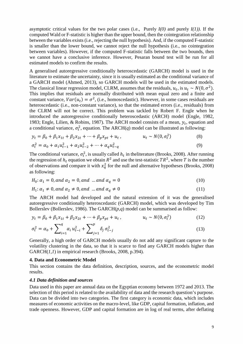
asymptotic critical values for the two polar cases (i.e., Purely I(0) and purely I(1)). If the computed Wald or F-statistic is higher than the upper bound, then the cointegration relationship between the variables exists (i.e., rejecting the null hypothesis). And, if the computed F-statistic is smaller than the lower bound, we cannot reject the null hypothesis (i.e., no cointegration between variables). However, if the computed F-statistic falls between the two bounds, then we cannot have a conclusive inference. However, Pesaran bound test will be run for all estimated models to confirm the results. A generalised autoregressive conditionally heteroscedastic (GARCH) model is used in the literature to estimate the uncertainty, since it is usually estimated as the conditional variance of a GARCH model (Ahmed, 2013), so GARCH models will be used in the estimated models. The classical linear regression model, CLRM, assumes that the residuals, 𝑢𝑢𝑖𝑖, is 𝑢𝑢𝑖𝑖 ∼ 𝑁𝑁(0,𝜎𝜎2). This implies that residuals are normally distributed with mean equal zero and a finite and constant variance, 𝑉𝑉𝑉𝑉𝑟𝑟(𝑢𝑢𝑖𝑖) = 𝜎𝜎2, (i.e., homoscedastic). However, in some cases residuals are heteroscedastic (i.e., non-constant variance), so that the estimated errors (i.e., residuals) from the CLRM will not be correct. This problem was tackled by Robert F. Engle when he introduced the autoregressive conditionally heteroscedastic (ARCH) model (Engle, 1982, 1983; Engle, Lilien, & Robins, 1987). The ARCH model consists of a mean, 𝑦𝑦𝑖𝑖, equation and a conditional variance, 𝜎𝜎𝑖𝑖2, equation. The ARCH(q) model can be illustrated as following:

𝑦𝑦𝑖𝑖 = 𝛽𝛽0 + 𝛽𝛽1𝑥𝑥1𝑖𝑖 + 𝛽𝛽2𝑥𝑥2𝑖𝑖 + ⋯+ 𝛽𝛽𝑝𝑝𝑥𝑥𝑝𝑝𝑖𝑖 + 𝑢𝑢𝑖𝑖 , 𝑢𝑢𝑖𝑖 ∼ 𝑁𝑁(0,𝜎𝜎𝑖𝑖2) (8)

𝜎𝜎𝑖𝑖2 = 𝛼𝛼0 + 𝛼𝛼1𝑢𝑢𝑖𝑖−12 + 𝛼𝛼2𝑢𝑢𝑖𝑖−22 + ⋯+ 𝛼𝛼𝑞𝑞𝑢𝑢𝑖𝑖−𝑞𝑞2 (9)

The conditional variance, 𝜎𝜎𝑖𝑖2, is usually called ℎ𝑖𝑖 in theliterature (Brooks, 2008). After running the regression of ℎ𝑖𝑖 equation we obtain 𝑅𝑅2 and use the test-statistic 𝑇𝑇𝑅𝑅2, where 𝑇𝑇 is the number of observations and compare it with 𝑥𝑥𝑞𝑞2 for the null and alternative hypotheses (Brooks, 2008) as following:

𝐻𝐻0: 𝛼𝛼1 = 0,𝑉𝑉𝑎𝑎𝑎𝑎 𝛼𝛼2 = 0,𝑉𝑉𝑎𝑎𝑎𝑎 … 𝑉𝑉𝑎𝑎𝑎𝑎 𝛼𝛼𝑞𝑞 = 0 (10)

𝐻𝐻1: 𝛼𝛼1 ≠ 0,𝑉𝑉𝑎𝑎𝑎𝑎 𝛼𝛼2 ≠ 0,𝑉𝑉𝑎𝑎𝑎𝑎 … 𝑉𝑉𝑎𝑎𝑎𝑎 𝛼𝛼𝑞𝑞 ≠ 0 (11)

The ARCH model had developed and the natural extension of it was the generalised autoregressive conditionally heteroscedastic (GARCH) model, which was developed by Tim Bollerslev (Bollerslev, 1986). The GARCH(p,q) model can be summarised as follow:

𝑦𝑦𝑖𝑖 = 𝛽𝛽0 + 𝛽𝛽1𝑥𝑥1𝑖𝑖 + 𝛽𝛽2𝑥𝑥2𝑖𝑖 + ⋯+ 𝛽𝛽𝑝𝑝𝑥𝑥𝑝𝑝𝑖𝑖 + 𝑢𝑢𝑖𝑖 , 𝑢𝑢𝑖𝑖 ∼ 𝑁𝑁(0,𝜎𝜎𝑖𝑖2) (12)

𝜎𝜎𝑖𝑖2 = 𝛼𝛼0 + � 𝛼𝛼𝑖𝑖𝑞𝑞

𝑖𝑖=1𝑢𝑢𝑖𝑖−𝑖𝑖2 + � 𝛿𝛿𝑗𝑗

𝑝𝑝

𝑗𝑗=1𝜎𝜎𝑖𝑖−𝑗𝑗2 (13)

Generally, a high order of GARCH models usually do not add any significant capture to the volatility clustering in the data, so that it is scarce to find any GARCH models higher than GARCH(1,1) in empirical research (Brooks, 2008, p.394).

4. Data and Econometric Model This section contains the data definition, description, sources, and the econometric model results.

4.1 Data definition and sources Data used in this paper are annual data on the Egyptian economy between 1972 and 2013. The selection of this period is related to the availability of data and the research question’s purpose. Data can be divided into two categories. The first category is economic data, which includes measures of economic activities on the macro-level, like GDP, capital formation, inflation, and trade openness. However, GDP and capital formation are in log of real terms, after deflating

9

nominal values by a GDP deflator. Additionally, the trade openness is calculated by dividing trade volume on GDP. Other variables (i.e., population and school enrolment) are a percentage from gross. All of these previous variables are defined according to the World Bank – World Development Indicators (WDI) Database. Additionally, investment data are in log of real term, after deflating nominal values by GDP deflator, and collected from the Egyptian Ministry of Planning (MoP) database. Table 1 is summarizes the variables’ symbols, definition and sources of data.

The second category of data is related to political variables3, which differ in measurement and source. The first source of political data is Freedom House’s Freedom in the World Country Ratings Database. Three variables are collected from this dataset (i.e., Political Rights and Civil Liberties, are measured on a one-to-seven scale, with one representing the highest degree of Freedom and seven the lowest). However, the Freedom Status, in case of Egypt, created as a dummy variable takes 1 for Partly Free and 0 for Not Free.4 The second source of political variables (i.e., Polity IV Regime Authority Characteristics and Transitions Datasets) is used to collect data about the assassination of executive and the resignation of executive. Assassination of executive is an indicator of the assassination of the ruling executive during the year of record5(see Marshall & Marshall, 2014). However, resignation of executive due to poor performance and/or loss of authority is defined as an indicator of the coerced resignation of the ruling executive due to poor performance and accompanied by increasing public discontent and popular demonstrations calling for the ouster of the executive leadership6(see Marshall & Marshall, 2014). Another index of political instability is government cabinet change (i.e., number of changes in the cabinet during the year), collected from the Egyptian Cabinet Records. Finally, a dummy variable that takes the value of 1 for 2011 and later, and 0 otherwise, which reflects the period after the 25th of January Revolution, is created by the author.

4.1.1 Political Instability Measures in Egypt This subsection briefly describes the measures of political instability in Egypt.

Government Change One of the used measures of political instability is government change, which reflects the number of changes in the government during one year. According to Figure 1 it is clear that in the 1980s five changes of government occurred, compared with only two during the 1990s. While in the 2000s, only one change occurred. However, in 2011 four changes occurred, and two changes happened between 2012 and 2013, which reflects the increasing trend in political instability. This increasing trend in government changes is related to the January 25 Revolution

Revolution Between 1952 and 2011 only two political revolutions occurred in Egypt. While, the 1952 revolution was led by Free Officers (i.e., an army revolution), the second in 2011 was led by the people. The 2011 revolution was sparked by the actions of youth who expressed their rejection of the unclear political vision, concentration of political power in the hand of one

3Carmignani (2003) indicated that the political instability index could include any of the socio-political unrest variables, like number of revolutions, political strikes, riots, number of coups, political assassination, and executions. 4Beginning with the ratings for 2003, countries whose combined average ratings fall between 3.0 and 5.0 are Partly Free and those between 5.5 and 7.0 are Not Free. 5 Assassinations are perpetrated by persons acting outside the ruling elite and do not result in a substantive change in regime leadership. 6Like assassinations, coerced resignations of an executive do not result in a substantive change in regime leadership, although they lead to new elections.

10

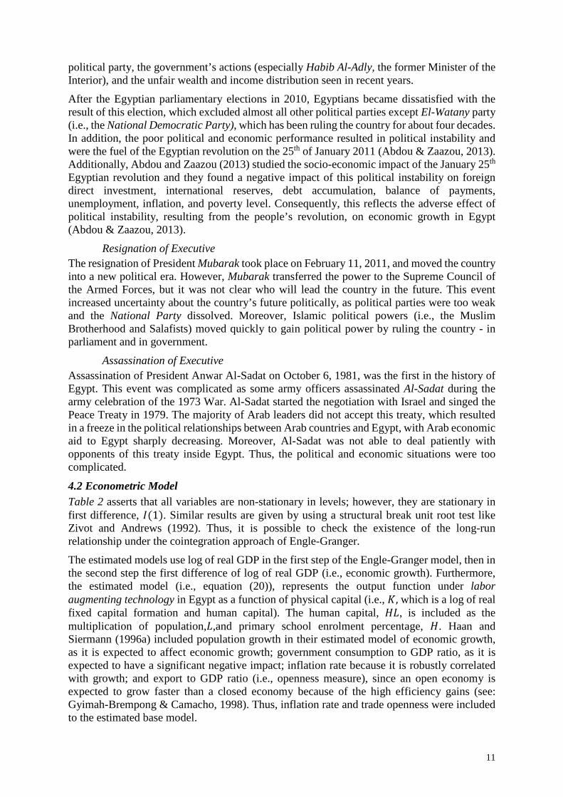
political party, the government’s actions (especially Habib Al-Adly, the former Minister of the Interior), and the unfair wealth and income distribution seen in recent years. After the Egyptian parliamentary elections in 2010, Egyptians became dissatisfied with the result of this election, which excluded almost all other political parties except El-Watany party (i.e., the National Democratic Party), which has been ruling the country for about four decades. In addition, the poor political and economic performance resulted in political instability and were the fuel of the Egyptian revolution on the 25th of January 2011 (Abdou & Zaazou, 2013). Additionally, Abdou and Zaazou (2013) studied the socio-economic impact of the January 25th Egyptian revolution and they found a negative impact of this political instability on foreign direct investment, international reserves, debt accumulation, balance of payments, unemployment, inflation, and poverty level. Consequently, this reflects the adverse effect of political instability, resulting from the people’s revolution, on economic growth in Egypt (Abdou & Zaazou, 2013).

Resignation of Executive The resignation of President Mubarak took place on February 11, 2011, and moved the country into a new political era. However, Mubarak transferred the power to the Supreme Council of the Armed Forces, but it was not clear who will lead the country in the future. This event increased uncertainty about the country’s future politically, as political parties were too weak and the National Party dissolved. Moreover, Islamic political powers (i.e., the Muslim Brotherhood and Salafists) moved quickly to gain political power by ruling the country - in parliament and in government.

Assassination of Executive Assassination of President Anwar Al-Sadat on October 6, 1981, was the first in the history of Egypt. This event was complicated as some army officers assassinated Al-Sadat during the army celebration of the 1973 War. Al-Sadat started the negotiation with Israel and singed the Peace Treaty in 1979. The majority of Arab leaders did not accept this treaty, which resulted in a freeze in the political relationships between Arab countries and Egypt, with Arab economic aid to Egypt sharply decreasing. Moreover, Al-Sadat was not able to deal patiently with opponents of this treaty inside Egypt. Thus, the political and economic situations were too complicated.

4.2 Econometric Model Table 2 asserts that all variables are non-stationary in levels; however, they are stationary in first difference, 𝐼𝐼(1). Similar results are given by using a structural break unit root test like Zivot and Andrews (1992). Thus, it is possible to check the existence of the long-run relationship under the cointegration approach of Engle-Granger. The estimated models use log of real GDP in the first step of the Engle-Granger model, then in the second step the first difference of log of real GDP (i.e., economic growth). Furthermore, the estimated model (i.e., equation (20)), represents the output function under labor augmenting technology in Egypt as a function of physical capital (i.e., 𝐾𝐾, which is a log of real fixed capital formation and human capital). The human capital, 𝐻𝐻𝐿𝐿, is included as the multiplication of population,𝐿𝐿,and primary school enrolment percentage, 𝐻𝐻. Haan and Siermann (1996a) included population growth in their estimated model of economic growth, as it is expected to affect economic growth; government consumption to GDP ratio, as it is expected to have a significant negative impact; inflation rate because it is robustly correlated with growth; and export to GDP ratio (i.e., openness measure), since an open economy is expected to grow faster than a closed economy because of the high efficiency gains (see: Gyimah-Brempong & Camacho, 1998). Thus, inflation rate and trade openness were included to the estimated base model.

11

The signs of variables are in line with the expectations of economic theory. Both physical and human capital have a positive effect on aggregate output, because the increase in those variables represents an increase in factors of production. However, the signs of inflation rate are negative, which could be explained by the negative impact of price level changes on real GDP (i.e., output and economic growth). Furthermore, the sign of trade openness is positive as explained by Gyimah-Brempong and Camacho (1998) and Haan and Siermann (1996a). The impact of physical and human capital on output is greater than the impact of inflation rate and trade openness, because the variables 𝐾𝐾 and 𝐻𝐻𝐿𝐿 are in logarithm scale.7

𝑌𝑌𝑖𝑖 = 19.801 + 0.102 𝐾𝐾𝑖𝑖 + 0.197 𝐻𝐻𝐿𝐿𝑖𝑖 − 0.0004 𝐼𝐼𝑎𝑎𝑓𝑓𝑖𝑖 + 0.342 𝑂𝑂𝑂𝑂𝑂𝑂𝑎𝑎𝑖𝑖 (14)

𝑇𝑇 = 37 𝑅𝑅2 = 0.962 𝑅𝑅𝑎𝑎𝑎𝑎𝑗𝑗2 = 0.958 𝑅𝑅𝑅𝑅𝑅𝑅 = 0.348 𝜎𝜎 = 0.104 𝐹𝐹 = 205.3[0.00]

Where𝑇𝑇 is the number of observations, 𝑅𝑅2 is the determination coefficient, 𝑅𝑅𝑎𝑎𝑎𝑎𝑗𝑗2 is adjusted determination coefficient, 𝑅𝑅𝑅𝑅𝑅𝑅 is residual sum square, 𝜎𝜎 is standard deviation, and 𝐹𝐹 is F-statistic. The second stage of the Engle-Granger approach is to use the residuals of the estimated model in an error-correction model, after testing the stationary of residuals. Consequently, the model’s residuals, 𝑢𝑢𝑖𝑖, will be used as the error correction mechanism (i.e., 𝐸𝐸𝐸𝐸𝐸𝐸). Furthermore, 𝐸𝐸𝐸𝐸𝐸𝐸 is stationary at 1% for DF-test and at 5% for ADF-test, with t-statistics equalling -4.464 and -2.592, respectively.

4.2.1 The uncertainty measures Uncertainty resulting from political instability could be estimated directly from the conditional variance of a political instability measure; however this is not possible for all political instability measures because of the low frequency and variations of values of these measures. Consequently, uncertainty level resulting from political instability could be measured indirectly by using the conditional variance of macroeconomic variables (i.e., income or price level), since political instability is affecting the economy through its impact on macroeconomic measures. The conditional variance of all political instability measures mentioned in Table 1 are used to construct the political uncertainty measure using a 𝐺𝐺𝐴𝐴𝑅𝑅𝐸𝐸𝐻𝐻 (1,1) model. However, none of these variables except civil liberties gives any plausible econometric results and they suffer non-normality. In case of 𝐸𝐸𝐿𝐿, the estimated model is (15), and it is well specified statistically: a moderate level of 𝑅𝑅2 and small RSS, normally distributed, and does not suffer from autocorrelation. Additionally, the conditional variance of civil liberties, ℎ𝑖𝑖𝐶𝐶𝐶𝐶, is significant, where standard errors, 𝑅𝑅𝐸𝐸, are in ( ) under the estimated coefficients. Moreover, ℎ𝑖𝑖𝐶𝐶𝐶𝐶 is stationary at 1%, because ADF-test is -10.117. 𝐸𝐸𝐿𝐿𝑖𝑖

(𝑅𝑅𝐸𝐸)= 1.376

(0.401)+ 0.921

(0.074)𝐸𝐸𝐿𝐿𝑖𝑖−1− 0.186

(0.094)𝐸𝐸𝐿𝐿𝑖𝑖−2

ℎ𝑖𝑖𝐶𝐶𝐶𝐶(𝑅𝑅𝐸𝐸)

= 0.058(0.010)

− 0.187(0.052)

𝑢𝑢𝑖𝑖−12 + 0.809(0.143)

ℎ𝑖𝑖−1𝐶𝐶𝐶𝐶

(15)

𝑅𝑅2 = 0.568𝑅𝑅𝑎𝑎𝑎𝑎𝑗𝑗2 = 0.544𝑅𝑅𝑅𝑅𝑅𝑅 = 9.069𝐴𝐴𝐼𝐼𝐸𝐸 = 1.142𝑅𝑅𝐼𝐼𝐸𝐸 = 1.395

𝐻𝐻𝐻𝐻𝐼𝐼𝐸𝐸 = 1.233 𝐹𝐹𝑎𝑎𝑎𝑎𝑎𝑎ℎ[1,37] = 0.058[0.51]𝜒𝜒𝑛𝑛𝑛𝑛𝑎𝑎2 [2] = 0.223[0.89]

7If transformation is used (i.e., the log scale transferred to normal scale), the coefficients of physical and human capital will be 1.107 and 1.218, respectively.

12

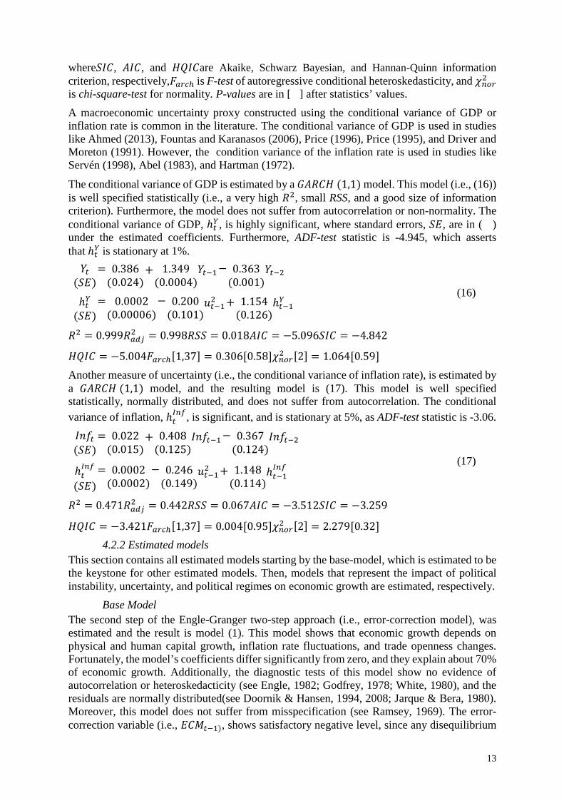
where𝑅𝑅𝐼𝐼𝐸𝐸, 𝐴𝐴𝐼𝐼𝐸𝐸, and 𝐻𝐻𝐻𝐻𝐼𝐼𝐸𝐸are Akaike, Schwarz Bayesian, and Hannan-Quinn information criterion, respectively,𝐹𝐹𝑎𝑎𝑎𝑎𝑎𝑎ℎ is F-test of autoregressive conditional heteroskedasticity, and 𝜒𝜒𝑛𝑛𝑛𝑛𝑎𝑎2 is chi-square-test for normality. P-values are in [ ] after statistics’ values. A macroeconomic uncertainty proxy constructed using the conditional variance of GDP or inflation rate is common in the literature. The conditional variance of GDP is used in studies like Ahmed (2013), Fountas and Karanasos (2006), Price (1996), Price (1995), and Driver and Moreton (1991). However, the condition variance of the inflation rate is used in studies like Servén (1998), Abel (1983), and Hartman (1972).

The conditional variance of GDP is estimated by a 𝐺𝐺𝐴𝐴𝑅𝑅𝐸𝐸𝐻𝐻 (1,1) model. This model (i.e., (16)) is well specified statistically (i.e., a very high 𝑅𝑅2, small RSS, and a good size of information criterion). Furthermore, the model does not suffer from autocorrelation or non-normality. The conditional variance of GDP, ℎ𝑖𝑖𝑌𝑌, is highly significant, where standard errors, 𝑅𝑅𝐸𝐸, are in ( ) under the estimated coefficients. Furthermore, ADF-test statistic is -4.945, which asserts that ℎ𝑖𝑖𝑌𝑌 is stationary at 1%. 𝑌𝑌𝑖𝑖

(𝑅𝑅𝐸𝐸)= 0.386

(0.024)+ 1.349

(0.0004)𝑌𝑌𝑖𝑖−1− 0.363

(0.001)𝑌𝑌𝑖𝑖−2

ℎ𝑖𝑖𝑌𝑌(𝑅𝑅𝐸𝐸)

= 0.0002(0.00006)

− 0.200(0.101)

𝑢𝑢𝑖𝑖−12 + 1.154(0.126)

ℎ𝑖𝑖−1𝑌𝑌

(16)

𝑅𝑅2 = 0.999𝑅𝑅𝑎𝑎𝑎𝑎𝑗𝑗2 = 0.998𝑅𝑅𝑅𝑅𝑅𝑅 = 0.018𝐴𝐴𝐼𝐼𝐸𝐸 = −5.096𝑅𝑅𝐼𝐼𝐸𝐸 = −4.842

𝐻𝐻𝐻𝐻𝐼𝐼𝐸𝐸 = −5.004𝐹𝐹𝑎𝑎𝑎𝑎𝑎𝑎ℎ[1,37] = 0.306[0.58]𝜒𝜒𝑛𝑛𝑛𝑛𝑎𝑎2 [2] = 1.064[0.59] Another measure of uncertainty (i.e., the conditional variance of inflation rate), is estimated by a 𝐺𝐺𝐴𝐴𝑅𝑅𝐸𝐸𝐻𝐻 (1,1) model, and the resulting model is (17). This model is well specified statistically, normally distributed, and does not suffer from autocorrelation. The conditional variance of inflation, ℎ𝑖𝑖

𝐼𝐼𝑛𝑛𝐼𝐼, is significant, and is stationary at 5%, as ADF-test statistic is -3.06. 𝐼𝐼𝑎𝑎𝑓𝑓𝑖𝑖(𝑅𝑅𝐸𝐸)

= 0.022(0.015)

+ 0.408(0.125)

𝐼𝐼𝑎𝑎𝑓𝑓𝑖𝑖−1− 0.367(0.124)

𝐼𝐼𝑎𝑎𝑓𝑓𝑖𝑖−2

ℎ𝑖𝑖𝐼𝐼𝑛𝑛𝐼𝐼

(𝑅𝑅𝐸𝐸)= 0.0002

(0.0002)− 0.246

(0.149)𝑢𝑢𝑖𝑖−12 + 1.148

(0.114)ℎ𝑖𝑖−1𝐼𝐼𝑛𝑛𝐼𝐼

(17)

𝑅𝑅2 = 0.471𝑅𝑅𝑎𝑎𝑎𝑎𝑗𝑗2 = 0.442𝑅𝑅𝑅𝑅𝑅𝑅 = 0.067𝐴𝐴𝐼𝐼𝐸𝐸 = −3.512𝑅𝑅𝐼𝐼𝐸𝐸 = −3.259

𝐻𝐻𝐻𝐻𝐼𝐼𝐸𝐸 = −3.421𝐹𝐹𝑎𝑎𝑎𝑎𝑎𝑎ℎ[1,37] = 0.004[0.95]𝜒𝜒𝑛𝑛𝑛𝑛𝑎𝑎2 [2] = 2.279[0.32] 4.2.2 Estimated models

This section contains all estimated models starting by the base-model, which is estimated to be the keystone for other estimated models. Then, models that represent the impact of political instability, uncertainty, and political regimes on economic growth are estimated, respectively.

Base Model The second step of the Engle-Granger two-step approach (i.e., error-correction model), was estimated and the result is model (1). This model shows that economic growth depends on physical and human capital growth, inflation rate fluctuations, and trade openness changes. Fortunately, the model’s coefficients differ significantly from zero, and they explain about 70% of economic growth. Additionally, the diagnostic tests of this model show no evidence of autocorrelation or heteroskedacticity (see Engle, 1982; Godfrey, 1978; White, 1980), and the residuals are normally distributed(see Doornik & Hansen, 1994, 2008; Jarque & Bera, 1980). Moreover, this model does not suffer from misspecification (see Ramsey, 1969). The error-correction variable (i.e., 𝐸𝐸𝐸𝐸𝐸𝐸𝑖𝑖−1), shows satisfactory negative level, since any disequilibrium

13

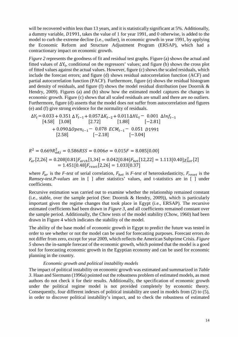
will be recovered within less than 13 years, and it is statistically significant at 5%. Additionally, a dummy variable, 𝐷𝐷1991, takes the value of 1 for year 1991, and 0 otherwise, is added to the model to curb the extreme decline (i.e., outlier), in economic growth in year 1991, by applying the Economic Reform and Structure Adjustment Program (ERSAP), which had a contractionary impact on economic growth. Figure 2 represents the goodness of fit and residual test graphs. Figure (a) shows the actual and fitted values of ∆Yt, conditional on the regressors’ values; and figure (b) shows the cross plot of fitted values against the actual values. However, figure (c) shows the scaled residuals, which include the forecast errors; and figure (d) shows residual autocorrelation function (ACF) and partial autocorrelation function (PACF). Furthermore, figure (e) shows the residual histogram and density of residuals, and figure (f) shows the model residual distribution (see Doornik & Hendry, 2009). Figures (a) and (b) show how the estimated model captures the changes in economic growth. Figure (c) shows that all scaled residuals are small and there are no outliers. Furthermore, figure (d) asserts that the model does not suffer from autocorrelation and figures (e) and (f) give strong evidence for the normality of residuals. ∆𝑌𝑌𝑖𝑖= 0.033

[4.58]+ 0.351

[3.08]∆𝑌𝑌𝑖𝑖−1+ 0.057

[2.72]∆𝐾𝐾𝑖𝑖−2+ 0.011

[1.88]∆𝐻𝐻𝐿𝐿𝑖𝑖− 0.001

[−2.81]∆𝐼𝐼𝑎𝑎𝑓𝑓𝑖𝑖−1

+ 0.090[2.58]

∆𝑂𝑂𝑂𝑂𝑂𝑂𝑎𝑎𝑖𝑖−1− 0.078[−2.18]

𝐸𝐸𝐸𝐸𝐸𝐸𝑖𝑖−1− 0.051[−3.04]

𝐷𝐷1991

𝑅𝑅2 = 0.669𝑅𝑅𝑎𝑎𝑎𝑎𝑗𝑗2 = 0.586𝑅𝑅𝑅𝑅𝑅𝑅 = 0.006𝜎𝜎 = 0.015𝐹𝐹 = 8.085[0.00]

𝐹𝐹𝑎𝑎𝑎𝑎[2,26] = 0.208[0.81]𝐹𝐹𝑎𝑎𝑎𝑎𝑎𝑎ℎ[1,34] = 0.042[0.84]𝐹𝐹ℎ𝑒𝑒𝑖𝑖[12,22] = 1.113[0.40]𝜒𝜒𝑛𝑛𝑛𝑛𝑎𝑎2 [2] = 1.451[0.48]𝐹𝐹𝑎𝑎𝑒𝑒𝑟𝑟𝑒𝑒𝑖𝑖[2,26] = 1.033[0.37]

where 𝐹𝐹𝑎𝑎𝑎𝑎 is the F-test of serial correlation, 𝐹𝐹ℎ𝑒𝑒𝑖𝑖 is F-test of heteroskedasticity, 𝐹𝐹𝑎𝑎𝑒𝑒𝑟𝑟𝑒𝑒𝑖𝑖 is the Ramsey-test.P-values are in [ ] after statistics’ values, and t-statistics are in [ ] under coefficients. Recursive estimation was carried out to examine whether the relationship remained constant (i.e., stable, over the sample period (See: Doornik & Hendry, 2009)), which is particularly important given the regime changes that took place in Egypt (i.e., ERSAP). The recursive estimated coefficients had been drawn in Figure 3, and all coefficients remained constant over the sample period. Additionally, the Chow tests of the model stability (Chow, 1960) had been drawn in Figure 4 which indicates the stability of the model. The ability of the base model of economic growth in Egypt to predict the future was tested in order to see whether or not the model can be used for forecasting purposes. Forecast errors do not differ from zero, except for year 2009, which reflects the American Subprime Crisis. Figure 5 shows the in-sample forecast of the economic growth, which pointed that the model is a good tool for forecasting economic growth in the Egyptian economy and can be used for economic planning in the country.

Economic growth and political instability models The impact of political instability on economic growth was estimated and summarized in Table 3. Haan and Siermann (1996a) pointed out the robustness problem of estimated models, as most authors do not check it for their results. Additionally, the specification of economic growth under the political regime model is not provided completely by economic theory. Consequently, four different indexes of political instability are used in models from (2) to (5), in order to discover political instability’s impact, and to check the robustness of estimated

14

models. The signs (i.e., directions) of all economic variables met the economic theory’s expectations. Previous economic growth affects the contemporaneous economic growth path positively and significantly at 1% for all models. The impact of lagged economic growth is between 33% and 39%, which means an increase by 100% in lagged economic growth will result in an increase in contemporaneous economic growth by 36% in average. Growth in physical capital formation is positively significant at 1% for all models, which means that an increase by 100% in physical capital will raise economic growth by 5.4% to 6.2%. Similarly, changes in human capital have a positive impact on economic growth between 1.0% and 1.3%, however in model (3) this impact is insignificant statistically. Inflation rate changes induce a negative impact on economic growth, about -0.1%, and it is significant statistically at 1% for all models, except model (5) since it is significant at 10%. Trade openness affects economic growth positively from 6.7% up to 9.1%, and its impact is significant at 5% for all models, except model (2) as it is significant at 1% level of significance.

The long-run relationship (i.e., 𝐸𝐸𝐸𝐸𝐸𝐸𝑖𝑖−1) exists in all estimated models, and is statistically significant except in model (3). The negative sign of 𝐸𝐸𝐸𝐸𝐸𝐸𝑖𝑖−1 in all models confirms that any divergence from equilibrium will be sorted out between less than 14 years in model (3), and less than 9 years in model (2), which reflects a plausible speed of adjustment. Additionally, the dummy variable (i.e., 𝐷𝐷1991) is significant at 1% and affects economic growth negatively, which reflects the contractionary impact of ERSAP on economic growth in Egypt. Political instability measured by Cabinet changes had a positive impact on economic growth. However, it is marginally significant at 10%. This result is supported by the results of Carmignani (2003), and it could be explained by Alesina et al. (1996). In the Egyptian case, governments do not change until people cannot accept them any longer. When that happens, the president starts to think about changing the government. People then have positive expectations about the future of the economy, which is encouraging economic growth by encouraging investment. Although, the 25th of January Revolution had a negative impact on economic growth as is expected, it is not significant. Similarly, resignation of executive (i.e., President Mubarak in early 2011), has a negative impact on economic growth according to the political instability induced by uncertainty of the future of the country, see Figure 6.

Furthermore, the variable 𝐴𝐴𝑠𝑠𝐸𝐸𝑥𝑥, which represents President Al-Sadat’s assassination on October 6, 1981, has a positive and significant impact on economic growth in the long-run, see Figure 7. This could be explained by the economic and political situation before and after Al-Sadat’s assassination. Before this event, Al-Sadat had political difficulties with internal and external political powers due to his position in Camp David in 1978 and the Peace Treaty in 1979 with Israel. This situation had developed when leaders of Arab countries cut their international relations with Egypt and stopped giving aid to Egypt (see Feiler, 2003). However, after this event president Mubarak tried to calm down the internal political conflicts and resume relations with Arab countries, which affected economic growth positively. These estimated models help explain between 67% and 75% of changes in economic growth in Egypt. Also, both 𝑅𝑅𝑅𝑅𝑅𝑅 and 𝜎𝜎 are relatively small. The diagnostic tests assert that the models do not suffer from autocorrelation and heteroscedasticity problems. Furthermore, these models follow the normal distribution and are well specified.

Economic growth and uncertainty models The impact of political instability on economic growth could be measured indirectly through the uncertainty level. Consequently, the impact of three uncertainty indexes generated using GARCH(1,1) (ℎ𝑖𝑖𝐶𝐶𝐶𝐶, ℎ𝑖𝑖𝑌𝑌, and ℎ𝑖𝑖

𝐼𝐼𝑛𝑛𝐼𝐼) were included to the base model, and the results were six models - from model (6) to model (11), which are summarized in Table 4. Similarly, the signs,

15

size of impact, and significance of all economic variables are per the theory’s expectations, and, in general, similar to those of political instability models. The variable 𝐷𝐷1991 is significant in all models except model (10), and it shows the negative impact of ERSAP on economic growth. The error-correction mechanism term is negative in all cases and at a reasonable level, where any disequilibrium will be recovered within range between less than 19 years in model (10), and less than 11 years in model (8). Furthermore, 𝐸𝐸𝐸𝐸𝐸𝐸𝑖𝑖−1is significant, which reflects the existence of the long-rum equilibrium, in all models except models (6) and (10). Moreover, the estimated models are able to explain between 48% and 76% of changes in economic growth in Egypt. Also, both 𝑅𝑅𝑅𝑅𝑅𝑅 and 𝜎𝜎 are relatively small. The diagnostic tests assert the existence of normality and statistical well-specified form, and absence of autocorrelation and heteroskedasticity. Figure 8 shows the co-movement between economic growth and uncertainty indexes. Moreover, models (6) and (7) assert the negative impact of uncertainty induced by political instability on economic growth, since variable ℎ𝑖𝑖𝐶𝐶𝐶𝐶 is used in model (6) in level and in model (7) in difference, and results show it is insignificant in model (7). However, model (7) is better than model (6) in estimating the long-run equilibrium relationship, since in this model the variable 𝐸𝐸𝐸𝐸𝐸𝐸𝑖𝑖−1 is statistically significant.

Additionally, models (8) and (9) used ℎ𝑖𝑖𝑌𝑌 as an uncertainty index, in level and in difference. However, model (9) provides results that are more plausible as the impact of ℎ𝑖𝑖𝐶𝐶𝐶𝐶 is negative. Similarly, variable ℎ𝑖𝑖

𝐼𝐼𝑛𝑛𝐼𝐼is used in models (10) and (11) to capture the impact of uncertainty on economic growth in the Egyptian economy. Although, both models assert the negative impact of uncertainty level on economic growth, model (11) is better as the uncertainty variable is highly significant. It is clear that using changes in uncertainty level gives more plausible results than using uncertainty index in level, as the changes in uncertainty play a distinct negative impact on economic growth.

Economic growth and democracy (political regime) models Political regime (i.e., democracy level) is expected to affect economic growth according to theory. In this way, three models, (12), (13), and (14), are estimated with three variables, which represent the democracy level (i.e., freedom level, political rights, and civil liberties). Table 5 shows the impact of democracy level on economic growth, with different indexes of democracy. These models are able to explain about 71% of changes in economic growth in Egypt. In addition, both 𝑅𝑅𝑅𝑅𝑅𝑅 and 𝜎𝜎 are relatively small, and diagnostic tests assert that models do not suffer from autocorrelation and heteroscedasticity problems. Furthermore, the models follow the normal distribution and are well specified. Also, according to these models, economic variables’ impact (i.e., direction, size of effect, and significance) on economic growth is in line with the expectations of economic theory. The long-run relationship exists in all of these estimated models, and is statistically significant at 5%. Moreover, the negative sign of 𝐸𝐸𝐸𝐸𝐸𝐸𝑖𝑖−1 and speed of adjustment assert that any disequilibrium will return to equilibrium after 12 years on average. Also, variable 𝐷𝐷1991 is significant at 1% and affects economic growth negatively in all models. Model (12) confirms the positive impact of democracy measured by degree of freedom on economic growth. This means that in periods of high political freedom, investment and economic growth increases. In Figure 9, the highlighted areas refer to years with a higher level of freedom, which are accompanied by higher economic growth. These results are similar to the results of Aisen and Veiga (2013). Additionally, model (13) asserts the positive impact of a high level of political rights on encouraging economic growth. The 𝑃𝑃𝑅𝑅 variable is measured on a one-to-seven scale, with one

16

representing the highest degree of freedom and seven the lowest. For this reason, the negative sign in this model represents the negative impact of low political rights on economic growth, see Figure 10. Similarly, the third measure of democracy (i.e., civil liberties) is used in model (14), and results assert the negative impact of low civil liberties on economic growth, where 𝐸𝐸𝐿𝐿 variable is measured as 𝑃𝑃𝑅𝑅 variable.

4.2.3 The Bounds Test The ARDL bounds test of Pesaran et al. (2001) is used to confirm the existence of the cointegration relationship between the variables in the economic growth models of the Egyptian economy during the last four decades. Table 6 summarizes the results of the pounds test for all estimated models. The bounds test highly confirm the existence of the long-run equilibrium relationship (i.e., cointegration) for all models at 1% level of significance, except for models (2) and (13) where they are significant at 5%.

5. Conclusion and Policy Recommendations This paper tried to provide an intensive study for the link between political dimension and economic growth. The economics literature does not provide a clear-cut understanding of the impact of political instability on economic growth, and the relationship between political system (i.e., level of democracy) and economic growth. Moreover, the impact of changes in uncertainty levels on economic growth are expected to be negative. Estimated models show the positive and significant impact of physical and human capital on economic growth in Egypt between 1972 and 2013. However, the effect of changes in physical capital on economic growth is higher than the impact of changes in human capital. Additionally, inflation rate fluctuations are responsible for a small and negative impact on economic growth in Egypt, and this impact is statistically significant. While, trade openness has a positive significant impact on economic growth, and its impact, in absolute value, is about nine times the impact of inflation. Furthermore, the economic reform (ERSAP) had a negative and significant impact on economic growth, especially at the start of its implementation in the early 1990s. Political instability measures show an ambiguous impact on economic growth in Egypt during the period of study. Different measures give different results. For example, both government change and assassination of executive (i.e., President Al-Sadat) have a positive and significant impact on economic growth, while both the January 25 Revolution and the resignation of executive (i.e., President Mubarak) have a negative and insignificant impact on economic growth. Consequently, the impact of political instability in Egypt will depend on the selected measure of political instability. Uncertainty level plays a significant role in determining the level of economic growth in Egypt; however, its impact is negative on economic growth, as all models of uncertainty show the adverse impact of a higher level of uncertainty induced by political or economic situations on economic growth in Egypt. The relationship between the level of democracy and economic growth in Egypt is confirmed. The higher level of freedom is associated with a higher level of economic growth. Similarly, a higher level of political rights and civil liberties stimulates investment and economic growth. It is clear that political stability, uncertainty, and democracy level are determining economic growth in Egypt. Thus, we cannot neglect their impact on real sector activities (i.e., investment decisions and economic growth). Additionally, I agree with Gyimah-Brempong and Camacho (1998) that in order to maintain sustainable economic development, policymakers should

17

widen their focus from only economic variables to include political and institutional variables that affect economic growth.

18

References Abdou, D. S., & Zaazou, Z. (2013). The Egyptian Revolution and post Socio-economic impact.

Topics in Middle Eastern and African Economies, 92-115. Abel, A. B. (1983). Optimal Investment Under Uncertainty. The American Economic Review,

73(1), 228-233. Ahmed, H. E. M. A. (2013). Investigating the Transmission Mechanism of Monetary Policy in

Egypt. (PhD), University of Birmingham, Birmingham, the UK. Aisen, A., & Veiga, F. J. (2013). How Does Political Instability Affect Economic Growth?

European Journal of Political Economy, 29, 151-167. Alesina, A., Özler, S., Roubini, N., & Swagel, P. (1996). Political Instability and Economic

Growth. Journal of Economic Growth, 1(2), 189-211. Barro, R. J. (1989). A Cross-Country Study of Growth, Saving, and Government: University of

Chicago Press. Barro, R. J., & Sala-i-Martin, X. (2004). Economic Growth (2 ed.). Cambridge: MIT Press. Bernal-Verdugo, L. E., Furceri, D., & Guillaume, D. M. (2013). The Dynamic Effect of Social

and Political Instability on Output: The Role of Reforms. IMF Working Paper. Research Department. International Monetary Fund (IMF). Washington, D. C.

Bollerslev, T. (1986). Generalized Autoregressive Conditional Heteroskedasticity. Journal of Econometrics, 31(3), 307-327.

Brooks, C. (2008). Introductory Econometrics for Finance (2 ed.). Cambridge: Cambridge University Press.

Brunetti, A., & Weder, B. (1995). Political Sources of Growth: A Critical Note on Measurement. Public Choice, 82(1/2), 125-134.

Campos, N. F., & Nugent, J. B. (2003). Aggregate Investment and Political Instability: An Econometric Investigation. Economica, 70(279), 533-549.

Carmignani, F. (2003). Political Instability, Uncertainty and Economics. Journal of Economic Surveys, 17(1), 1-54.

Carruth, A., Dickerson, A., & Henley, A. (2000). What Do We Know about Investment Under Uncertainty? Journal of Economic Surveys, 14(2), 119-154.

Chow, G. C. (1960). Tests of Equality Between Sets of Coefficients in Two Linear Regressions. Econometrica, 28(3), 591-605.

Dickey, D. A., & Fuller, W. A. (1979). Distribution of the Estimators for Autoregressive Time Series With a Unit Root. Journal of the American Statistical Association, 74(366), 427-431.

Doornik, J. A., & Hansen, H. (1994). An Omnibus Test for Univariate and Multivariate Normality. . Economic Discussion Paper. University of Oxford. Oxford

Doornik, J. A., & Hansen, H. (2008). An Omnibus Test for Univariate and Multivariate Normality. Oxford Bulletin of Economics and Statistics, 70(s1), 927-939.

Doornik, J. A., & Hendry, D. F. (2009). Empirical Econometric Modelling PcGive 13: Volume I (Vol. Volume I). London: Timberlake Consultants Ltd.

Driver, C., & Moreton, D. (1991). The Influence of Uncertainty on UK Manufacturing Investment. The Economic Journal, 101(409), 1452-1459.

19

Engle, R. F. (1982). Autoregressive Conditional Heteroscedasticity with Estimates of the Variance of United Kingdom Inflation. Econometrica, 50(4), 987-1007.

Engle, R. F. (1983). Estimates of the Variance of US Inflation Based upon the ARCH Model. Journal of Money, Credit and Banking, 15(3), 286-301.

Engle, R. F., Lilien, D. M., & Robins, R. P. (1987). Estimating Time Varying Risk Premia in the Term Structure: The ARCH-M Model. Econometrica: Journal of the Econometric Society, 391-407.

Feiler, G. (2003). Economic Relations between Egypt and the Gulf Oil States, 1967-2000: Petro-Wealth and Patterns of Influence. Brighton: Sussex Academic Press.

Ferderer, J. P. (1993). The Impact of Uncertainty on Aggregate Investment Spending: An Empirical Analysis. Journal of Money, Credit and Banking, 25(1), 30-48.

Fielding, D., & Shortland, A. (2005). Political Violence and Excess Liquidity in Egypt. Journal of Development Studies, 41(4), 542-557.

Fosu, A. K. (1992). Political Instability and Economic Growth: Evidence from Sub-Saharan Africa. Economic Development and Cultural Change, 40(4), 829-841.

Fosu, A. K. (2002). Political Instability and Economic Growth: Implications of Coup Events in Sub-Saharan Africa. American Journal of Economics and Sociology, 61(1), 329-348.

Fountas, S., & Karanasos, M. (2006). The Relationship between Economic Growth and Real Uncertainty in the G3. Economic Modelling, 23(4), 638-647.

Godfrey, L. G. (1978). Testing for Multiplicative Heteroskedasticity. Journal of Econometrics, 8(2), 227-236.

Granger, C. W. J. (1966). The Typical Spectral Shape of an Economic Variable. Econometrica, 34(1), 150-161.

Granger, C. W. J., & Newbold, P. (1974). Spurious Regressions in Econometrics. Journal of Econometrics, 2(2), 111-120.

Gyimah-Brempong, K., & Camacho, S. M. D. (1998). Political Instability, Human Capital, and Economic Growth in Latin America. The Journal of Developing Areas, 32(4), 449-466.

Haan, J. d., & Siermann, C. L. J. (1996a). New Evidence on the Relationship between Democracy and Economic Growth. Public Choice, 86(1/2), 175-198.

Haan, J. d., & Siermann, C. L. J. (1996b). Political Instability, Freedom, and Economic Growth: Some Further Evidence. Economic Development and Cultural Change, 44(2), 339-350.

Hartman, R. (1972). The Effects of Price and Cost Uncertainty on Investment. Journal of Economic Theory, 5(2), 258-266.

Ingersoll Jr, J. E., & Ross, S. A. (1992). Waiting to Invest: Investment and Uncertainty. Journal of Business, 1-29.

Jarque, C. M., & Bera, A. K. (1980). Efficient Tests for Normality, Homoscedasticity and Serial Independence of Regression Residuals. Economics Letters, 6(3), 255-259.

Jong-A-Pin, R. (2009). On the Measurement of Political Instability and Its Impact on Economic Growth. European Journal of Political Economy, 25(1), 15-29.

Kwiatkowski, D., Phillips, P. C. B., Schmidt, P., & Shin, Y. (1992). Testing the null hypothesis of stationarity against the alternative of a unit root: How sure are we that economic time series have a unit root? Journal of Econometrics, 54(1–3), 159-178. doi: 10.1016/0304-4076(92)90104-y

20

MacKinnon, J. G. (2010). Critical Values for Cointegration Tests. Working Paper. Department of Economics. Queen’s University. Canada.

Marshall, M. G., & Marshall, D. R. (2014). Coup d'etat Events 1946-2013 Coodbook Polity IV Regime Authority Characteristics and Transitions Datasets: Center for Systemic Peace

Nelson, C. R., & Plosser, C. R. (1982). Trends and Random Walks in Macroeconomic Time Series: Some Evidence and Implications. Journal of Monetary Economics, 10(2), 139-162.

Pesaran, M. H., & Shin, Y. (1999). An Autoregressive Distributed Lag Modelling Approach to Cointegration Analysis. In S. Strom (Ed.), Econometrics and Economic Theory in the 20th Century, The Ragnar Frisch Centennial Symposium (pp. 371-413 ). Cambridge: Cambridge University Press.

Pesaran, M. H., Shin, Y., & Smith, R. J. (2001). Bounds Testing Approaches to the Analysis of Level Relationships. Journal of Applied Econometrics, 16(3), 289-326.

Phillips, P. C. B., & Perron, P. (1988). Testing for a Unit Root in Time Series Regression. Biometrika, 75(2), 335-346.

Plümper, T., & Martin, C. W. (2003). Democracy, Government Spending, and Economic Growth: A Political-Economic Explanation of the Barro-Effect. Public Choice, 117(1/2), 27-50.

Price, S. (1995). Aggregate Uncertainty, Capacity Utilization and Manufacturing Investment. Applied Economics, 27(2), 147-154.

Price, S. (1996). Aggregate Uncertainty, Investment and Asymmetric Adjustment in the UK Manufacturing Sector. Applied Economics, 28(11), 1369-1379.

Ramsey, J. B. (1969). Tests for Specification Errors in Classical Linear Least-Squares Regression Analysis. Journal of the Royal Statistical Society. Series B (Methodological), 31(2), 350-371.

Romer, D. (2012). Advanced Macroeconomics (4 Ed ed.). New York: McGraw-Hill Irwin. Scully, G. W. (1988). The Institutional Framework and Economic Development. Journal of

Political Economy, 96(3), 652-662. Servén, L. (1998). Macroeconomic Uncertainty and Private Investment in Developing

Countries: An empirical Investigation. World Bank Policy Research Working Paper No. 2035.

Solow, R. M. (1956). A Contribution to the Theory of Economic Growth. The Quarterly Journal of Economics, 70(1), 65-94.

Svensson, J. (1998). Investment, Property Rights and Political Instability: Theory and Evidence. European Economic Review, 42(7), 1317-1341.

Swan, T. W. (1956). Economic Growth and Capital Accumulation. Economic Record, 32(2), 334-361.

Verbeek, M. (2007). A Guide to Modern Econometrics (2 ed.). New York: John Wiley & Sons, Ltd.

White, H. (1980). A Heteroskedasticity-Consistent Covariance Matrix Estimator and a Direct Test for Heteroskedasticity. Econometrica: Journal of the Econometric Society, 817-838.

Zivot, E., & Andrews, D. W. K. (1992). Further Evidence on the Great Crash, the Oil-Price Shock, and the Unit-Root Hypothesis. Journal of Business & Economic Statistics, 10(3), 251-270.

21

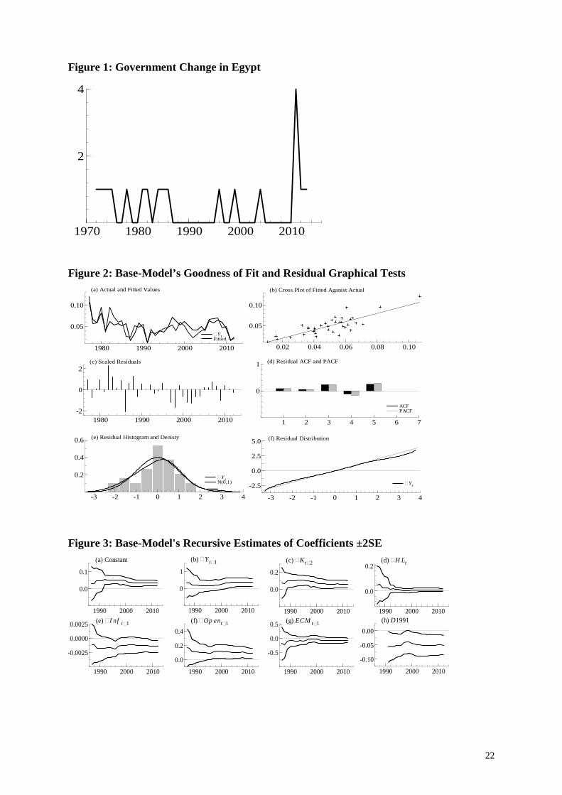
Figure 1: Government Change in Egypt

Figure 2: Base-Model’s Goodness of Fit and Residual Graphical Tests

Figure 3: Base-Model's Recursive Estimates of Coefficients ±2SE

1970 1980 1990 2000 2010

2

4

DYt Fitted

1980 1990 2000 2010

0.05

0.10

(a) Actual and Fitted Values

DYt Fitted

0.02 0.04 0.06 0.08 0.10

0.05

0.10

(b) Cross Plot of Fitted Aganist Actual

1980 1990 2000 2010-2

0

2(c) Scaled Residuals

-3 -2 -1 0 1 2 3 4

0.2

0.4

0.6 (e) Residual Histogram and Denisty

DYt N(0,1)

ACF PACF

1 2 3 4 5 6 7

0

1 (d) Residual ACF and PACF

ACF PACF

DYt

-3 -2 -1 0 1 2 3 4

-2.5

0.0

2.5

5.0 (f) Residual Distribution

DYt

1990 2000 2010

0

1

(b) DYtD1

1990 2000 2010

0.0

0.1

(a) Constant

1990 2000 2010

0.0

0.2

(c) DKtD2

1990 2000 2010

0.0

0.2(d) DH Lt

1990 2000 2010

-0.0025

0.0000

0.0025 (e) DI nf tD1

1990 2000 2010

0.0

0.2

0.4(f) DOp entD1

1990 2000 2010

-0.5

0.0

0.5 (g) ECM tD1

1990 2000 2010

-0.10

-0.05

0.00(h) D1991

22

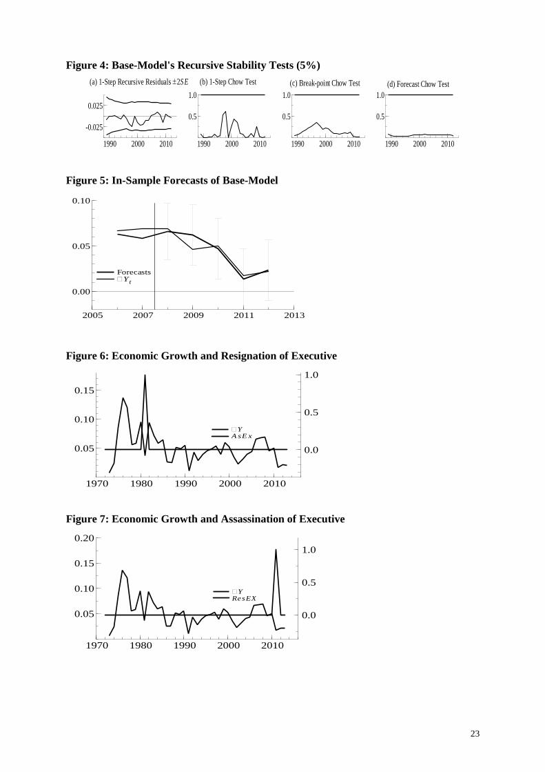
Figure 4: Base-Model's Recursive Stability Tests (5%)

Figure 5: In-Sample Forecasts of Base-Model

Figure 6: Economic Growth and Resignation of Executive

Figure 7: Economic Growth and Assassination of Executive

1990 2000 2010

-0.025

0.025

(a) 1-Step Recursive Residuals ±2S E

1990 2000 2010

0.5

1.0(b) 1-Step Chow Test

1990 2000 2010

0.5

1.0(c) Break-point Chow Test

1990 2000 2010

0.5

1.0(d) Forecast Chow Test

Forecasts DYt

2005 2007 2009 2011 2013

0.00

0.05

0.10

Forecasts DYt

DY A sE x

0.05

0.10

0.15

0.0

0.5

1.0

1970 1980 1990 2000 2010

DY A sE x

DY ResEX

0.05

0.10

0.15

0.20

0.0

0.5

1.0

1970 1980 1990 2000 2010

DY ResEX

23

Figure 8: Economic Growth and Uncertainty

Figure 9: Economic Growth and Democracy

Figure 10: Economic Growth and Political Rights

Figure 11: Economic Growth and Civil Liberties

DYt hY

0.05

0.10

0.15

0.0000

0.0005

0.0010

1980 1990 2000 2010

(a) Economic Growth and Uncertainity of Income

DYt hY DYt hI nf

0.05

0.10

0.002

1980 1990 2000 2010

(b) Economic Growth and Uncertainity of Inflation

DYt hI nf DYt hC L

0.05

0.10

0.15

0.0

0.5

1980 1990 2000 2010

(c) Economic Growth and Uncertainity of Political Regime

DYt hC L

DYt F ree

0.05

0.10

0.5

1.0

1975 1985 1995 2005 2015

DYt F ree

DYt PR

0.0

0.1

4

6

1975 1985 1995 2005 2015

DYt PR

DYt C Lt

0.00

0.05

0.10

4

5

6

1975 1985 1995 2005 2015

DYt C Lt

24

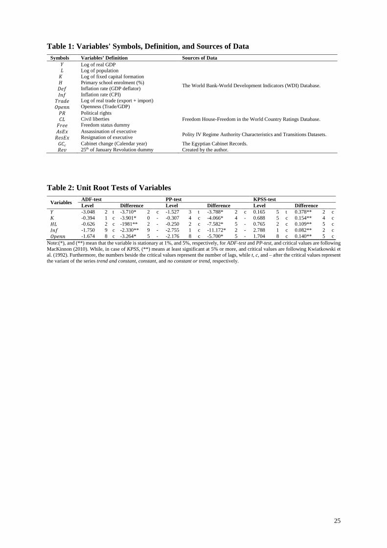
Table 1: Variables' Symbols, Definition, and Sources of Data Symbols Variables’ Definition Sources of Data

𝑌𝑌 𝐿𝐿 𝐾𝐾 𝐻𝐻 𝐷𝐷𝑂𝑂𝑓𝑓 𝐼𝐼𝑎𝑎𝑓𝑓 𝑇𝑇𝑟𝑟𝑉𝑉𝑎𝑎𝑂𝑂 𝑂𝑂𝑂𝑂𝑂𝑂𝑎𝑎𝑎𝑎

Log of real GDP Log of population Log of fixed capital formation Primary school enrolment (%) Inflation rate (GDP deflator) Inflation rate (CPI) Log of real trade (export + import) Openness (Trade/GDP)

The World Bank-World Development Indicators (WDI) Database.

𝑃𝑃𝑅𝑅 𝐸𝐸𝐿𝐿 𝐹𝐹𝑟𝑟𝑂𝑂𝑂𝑂

Political rights Civil liberties Freedom status dummy

Freedom House-Freedom in the World Country Ratings Database.

𝐴𝐴𝑠𝑠𝐸𝐸𝑥𝑥 𝑅𝑅𝑂𝑂𝑠𝑠𝐸𝐸𝑥𝑥

Assassination of executive Resignation of executive Polity IV Regime Authority Characteristics and Transitions Datasets.

𝐺𝐺𝐸𝐸𝑎𝑎 Cabinet change (Calendar year) The Egyptian Cabinet Records. 𝑅𝑅𝑂𝑂𝑅𝑅 25th of January Revolution dummy Created by the author.

Table 2: Unit Root Tests of Variables

Variables ADF-test PP-test KPSS-test Level Difference Level Difference Level Difference

𝑌𝑌 -3.048 2 t -3.710* 2 c -1.527 3 t -3.788* 2 c 0.165 5 t 0.378** 2 c K -0.394 1 c -3.901* 0 - -0.307 4 c -4.066* 4 - 0.688 5 c 0.154** 4 c 𝐻𝐻𝐿𝐿 -0.626 2 c -1981** 2 - -0.250 2 c -7.582* 5 - 0.765 2 c 0.109** 5 c 𝐼𝐼𝑎𝑎𝑓𝑓 -1.750 9 c -2.330** 9 - -2.755 1 c -11.172* 2 - 2.788 1 c 0.082** 2 c 𝑂𝑂𝑂𝑂𝑂𝑂𝑎𝑎𝑎𝑎 -1.674 8 c -3.264* 5 - -2.176 8 c -5.700* 5 - 1.704 8 c 0.140** 5 c

Note:(*), and (**) mean that the variable is stationary at 1%, and 5%, respectively, for ADF-test and PP-test, and critical values are following MacKinnon (2010). While, in case of KPSS, (**) means at least significant at 5% or more, and critical values are following Kwiatkowski et al. (1992). Furthermore, the numbers beside the critical values represent the number of lags, while t, c, and – after the critical values represent the variant of the series trend and constant, constant, and no constant or trend, respectively.

25

Table 3: Impact of Political Instability on Economic Growth

Variables ∆𝒀𝒀𝒕𝒕 (2) (3) (4) (5)

Constant 0.026* [3.25]

0.033* [4.29]

0.033* [4.30]

0.033* [5.20]

∆𝑌𝑌𝑖𝑖−1 0.390* [3.43]

0.348* [2.97]

0.342* [2.84]

0.329* [3.26]

∆𝐾𝐾𝑖𝑖−2 0.054* [2.58]

0.057* [2.67]

0.059* [2.68]

0.062* [3.33]

∆𝐻𝐻𝐿𝐿𝑖𝑖−1 0.013** [2.17]

0.010 [1.48]

0.010*** [1.75]

0.010** [1.97]

∆𝐼𝐼𝑎𝑎𝑓𝑓𝑖𝑖−1 -0.001* [-2.77]

-0.001* [-2.76]

-0.001* [-2.77]

-0.001*** [-1.83]

∆𝑂𝑂𝑂𝑂𝑂𝑂𝑎𝑎𝑖𝑖−1 0.089* [2.62]

0.089** [2.52]

0.091** [2.55]

0.067** [2.10]

𝐸𝐸𝐸𝐸𝐸𝐸𝑖𝑖−1 -0.115* [-2.67]

-0.073 [-1.54]

-0.073*** [-1.74]

-0.087* [-2.73]

𝐷𝐷1991 -0.053* [-3.20]

-0.050* [-2.87]

-0.050* [-2.89]

-0.046* [-3.08]

𝐺𝐺𝐸𝐸𝑖𝑖 0.003 [0.818]

𝐺𝐺𝐸𝐸𝑖𝑖−1 0.007 [1.69]

𝑅𝑅𝑂𝑂𝑅𝑅𝑖𝑖 -0.002 [-0.17]

𝑅𝑅𝑂𝑂𝑠𝑠𝐸𝐸𝑥𝑥𝑖𝑖−1 -0.005 [-0.27]

𝐴𝐴𝑠𝑠𝐸𝐸𝑥𝑥𝑖𝑖−1 0.044* [2.99]

Goodness of Fit Measures 𝑇𝑇 36 36 36 36 𝑅𝑅2 0.705 0.669 0.670 0.751 𝑅𝑅𝑎𝑎𝑎𝑎𝑗𝑗2 0.602 0.571 0.572 0.677 𝑅𝑅𝑅𝑅𝑅𝑅 0.005 0.006 0.006 0.004 𝜎𝜎 0.014 0.015 0.015 0.013 𝐹𝐹 6.902

[0.00] 6.833 [0.00]

6.85 [0.00]

10.19 [0.00]

Diagnostic Tests 𝐹𝐹𝑎𝑎𝑎𝑎 0.148

[0.86] 0.195 [0.82]

0.245 [0.78]

0.093 [0.91]

𝐹𝐹𝑎𝑎𝑎𝑎𝑎𝑎ℎ 0.004 [0.95]

0.029 [0.87]

0.031 [0.86]

0.526 [0.47]

𝐹𝐹ℎ𝑒𝑒𝑖𝑖 1.920 [0.10]

0.953 [0.52]

0.970 [0.50]

0.490 [0.90]

𝜒𝜒𝑛𝑛𝑛𝑛𝑎𝑎2 2.435 [0.30]

1.365 [0.51]

1.307 [0.52]

1.132 [0.57]

𝐹𝐹𝑎𝑎𝑒𝑒𝑟𝑟𝑒𝑒𝑖𝑖 0.669 [0.52]

1.454 [0.25]

1.273 [0.30]

1.063 [0.36]

Note: t-values are under the coefficients and between [ ], while, (*), (**), (***) mean that the variable is statistically significant at 1%, 5%, and 10%, respectively. Also, 𝑂𝑂 − 𝑅𝑅𝑉𝑉𝑣𝑣𝑢𝑢𝑂𝑂 is under diagnostic tests’ statistics between [ ].

26

Table 4: Impact of Uncertainty on Economic Growth

Variables ∆𝒀𝒀𝒕𝒕 (6) (7) (8) (9) (10) (11)

Constant 0.045* [4.66] 0.033* [4.64 ] 0.034* [4.96] 0.032*[5.02] 0.039* [3.93] 0.030* [4.85]

∆𝑌𝑌𝑖𝑖−1 0.324* [2.93]

0.332* [2.87] 0.162 [1.10] 0.315*[3.04 ] 0.254 [1.61] 0.414*

[4.11]

∆𝐾𝐾𝑖𝑖−2 0.063* [3.06] 0.051** [2.33] 0.058* [2.88] 0.050*[2.59] 0.067* [2.72] 0.061* [3.36]

∆𝐻𝐻𝐿𝐿𝑖𝑖−1 0.009 [1.55] 0.010*** [1.84 ] 0.012** [2.19] 0.012**[2.26 ] 0.005 [0.657] 0.007 [1.41]

∆𝐼𝐼𝑎𝑎𝑓𝑓𝑖𝑖−1 -0.002* [-3.37]

-0.001* [-2.86]

-0.001* [-2.68]

-0.002* [-3.48] -0.0005

[-0.91]

∆𝑂𝑂𝑂𝑂𝑂𝑂𝑎𝑎𝑖𝑖−1 0.085** [2.53]

0.095* [2.70 ] 0.058 [1.54] 0.100*[3.18] 0.087**

[1.93] 0.117* [3.74]

𝐸𝐸𝐸𝐸𝐸𝐸𝑖𝑖−1 -0.055 [-1.48]

-0.071*** [-1.91]

-0.097* [-2.71]

-0.065** [ -1.99 ]

-0.054 [-1.25]

-0.063** [-1.99]

𝐷𝐷1991 -0.046* [-2.78]

-0.051* [-3.03]

-0.055* [-3.40]

-0.047* [ -3.10]

-0.002 [-0.105]

-0.046* [-3.14]

ℎ𝑖𝑖−2𝐶𝐶𝐶𝐶 -0.089*** [-1.82]

∆ℎ𝑖𝑖−2𝐶𝐶𝐶𝐶 -0.022 [-0.96]

ℎ𝑖𝑖𝑌𝑌 33.641*** [1.91]

∆ℎ𝑖𝑖𝑌𝑌 -58.84*[-2.72]

ℎ𝑖𝑖−1𝐼𝐼𝑛𝑛𝐼𝐼 -0.056

[-0.012]

∆ℎ𝑖𝑖𝐼𝐼𝑛𝑛𝐼𝐼 -14.004* [-

3.22] Goodness of Fit Measures 𝑇𝑇 36 36 36 36 36 36 𝑅𝑅2 0.705 0.680 0.708 0.740 0.484 0.761 𝑅𝑅𝑎𝑎𝑎𝑎𝑗𝑗2 0.618 0.585 0.622 0.663 0.355 0.690 𝑅𝑅𝑅𝑅𝑅𝑅 0.005 0.006 0.005 0.005 0.009 0.004 𝜎𝜎 0.014 0.015 0.014 0.013 0.018 0.013

𝐹𝐹 8.072 [0.00]

7.166 [0.00] 8.202 [0.00] 9.615 [0.00] 3.755 [0.01] 10.73 [0.00]

Diagnostic Tests

𝐹𝐹𝑎𝑎𝑎𝑎 0.821 [0.45] 0.356 [0.70] 0.763 [0.48] 0.012 [0.99] 0.153 [0.86] 0.577 [0.57]

𝐹𝐹𝑎𝑎𝑎𝑎𝑎𝑎ℎ 0.479 [0.49] 0.211 [0.65] 0.157 [0.69] 0.176 [0.68] 0.115 [0.74] 0.125 [0.73] 𝐹𝐹ℎ𝑒𝑒𝑖𝑖 0.903 [0.57] 0.762 [0.69] 1.056 [0.45] 0.883 [0.59] 0.361 [0.96] 0.608 [0.83] 𝜒𝜒𝑛𝑛𝑛𝑛𝑎𝑎2 0.362 [0.83] 1.196 [0.55] 2.929 [0.23] 0.626 [0.73] 5.698 [0.06] 2.413 [0.30] 𝐹𝐹𝑎𝑎𝑒𝑒𝑟𝑟𝑒𝑒𝑖𝑖 0.584 [0.56] 0.807 [0.46] 0.727 [0.49] 0.828 [0.45] 1.312 [0.29] 2.226 [0.13]

Note: t-values are under the coefficients and between [ ], while, (*), (**), (***) mean that the variable is statistically significant at 1%, 5%, and 10%, respectively. Also, 𝑂𝑂 − 𝑅𝑅𝑉𝑉𝑣𝑣𝑢𝑢𝑂𝑂 is under diagnostic tests’ statistics between [ ].

27

Table 5: Impact of Democracy (Political Regime) on Economic Growth

Variables ∆𝑌𝑌𝑖𝑖 (12) (13) (14)

Constant 0.032* [4.86]

0.083* [3.31]

0.069* [3.31]

∆𝑌𝑌𝑖𝑖−1 0.268** [2.36]

0.283** [2.52]

0.292** [2.56]

∆𝐾𝐾𝑖𝑖−2 0.066* [3.29]

0.063* [3.13]

0.060* [2.96]

∆𝐻𝐻𝐿𝐿𝑖𝑖−1 0.010*** [1.94]

0.010*** [1.90]

0.010*** [1.76]

∆𝐼𝐼𝑎𝑎𝑓𝑓𝑖𝑖−1 -0.002* [-3.16]

-0.002* [-3.10]

-0.002* [-3.08]

∆𝑂𝑂𝑂𝑂𝑂𝑂𝑎𝑎𝑖𝑖−1 0.083** [2.52]

0.087* [2.65]

0.092* [2.76]

𝐸𝐸𝐸𝐸𝐸𝐸𝑖𝑖−1 -0.082** [-2.44]

-0.082** [-2.43]

-0.078** [-2.26]

𝐷𝐷1991 -0.055* [-3.47]

-0.054* [-3.40]

-0.051* [-3.14]

𝐹𝐹𝑟𝑟𝑂𝑂𝑂𝑂𝑖𝑖 0.011** [2.18]

𝑃𝑃𝑅𝑅𝑖𝑖 -0.009 ** [-2.09]

𝐸𝐸𝐿𝐿𝑖𝑖−1 -0.007*** [-1.85]

Goodness of Fit Measures 𝑇𝑇 36 36 36 𝑅𝑅2 0.719 0.715 0.706 𝑅𝑅𝑎𝑎𝑎𝑎𝑗𝑗2 0.635 0.631 0.619 𝑅𝑅𝑅𝑅𝑅𝑅 0.005 0.005 0.005 𝜎𝜎 0.014 0.014 0.014

𝐹𝐹 8.624 [0.00]

8.472 [0.00]

8.120 [0.00]

Diagnostic Tests

𝐹𝐹𝑎𝑎𝑎𝑎 0.160 [0.85]

0.277 [0.76]

0.217 [0.81]

𝐹𝐹𝑎𝑎𝑎𝑎𝑎𝑎ℎ 0.287 [0.60]

0.227 [0.64]

0.059 [0.81]

𝐹𝐹ℎ𝑒𝑒𝑖𝑖 0.832 [0.63]

1.085 [0.42]

0.793 [0.67]

𝜒𝜒𝑛𝑛𝑛𝑛𝑎𝑎2 3.597 [0.17]

2.619 [0.27]

7.007 [0.03]

𝐹𝐹𝑎𝑎𝑒𝑒𝑟𝑟𝑒𝑒𝑖𝑖 0.715 [0.50]

0.956 [0.40]

0.795 [0.46]

Note: t-values are under the coefficients and between [ ], while, (*), (**), (***) mean that the variable is statistically significant at 1%, 5%, and 10%, respectively. Also, 𝑂𝑂 − 𝑅𝑅𝑉𝑉𝑣𝑣𝑢𝑢𝑂𝑂 is under diagnostic tests’ statistics between [ ].

Table 6: Results of the Bound Tests

Type Model No. F-statistic P-value

CI(ii) CI(iii) Upper bound

Lower bound

Upper bound

Lower bound

Base-Model (1) 6.779* [0.000] 3.99 2.88 4.43 3.15

Political Instability Models

(2) 3.895** [0.010] 3.28 2.27 3.16 2.45 (3) 6.320* [0.001]

3.99 2.88 4.43 3.15

(4) 6.089* [0.001] (5) 6.159* [0.001]

Uncertainty Models

(6) 7.975* [0.000] (7) 7.159* [0.000] (8) 6.188* [0.001] (9) 6.208* [0.001]

(10) 8.430* [0.000] (11) 7.390* [0.000]

Political Regime (Democracy) Models

(12) 5.662* [0.001] (13) 3.373** [0.016] 3.28 2.27 3.16 2.45 (14) 4.734* [0.003] 3.99 2.88 4.43 3.15

Note: The critical values are obtained from Pesaran et al. (2001), where CI(ii) is restricted intercept and no trend case and CI(iii) is unrestricted intercept and no trend case. In addition, p-values are between [ ].Also, * and ** mean significant at 1% and 5%, respectively.

28