Political economy of land use and logging in presence of externalities

Author:

Johanna Jussila University of Gothenburg

Sweden

Political Economy of Land Use and Logging in Presence of Externalities

Johanna Jussila

Department of Economics

School of Economics and Commercial Law, University of Gothenburg

August 19, 2003

Abstract:

This paper develops a political economy model with menu auctions between a

government and lobbies to determine the environmental policy. Two of the (three)

production sectors share a common sector-specific factor of production, namely land,

which has two externalities connected to it: a positive one arising from forest

amenities and a negative one arising from logging. The government has two policy

instruments at its disposal: a land tax-cum-subsidy and a production tax-cum-subsidy.

The interdependence between the two land using sectors is shown to impact the

setting of respective land tax-cum-subsidy. Consequently, land use in logging will be

subsidized and that in agriculture will be taxed. Production of logs will be taxed.

Moreover, the paper also studies the effect of property rights. It is found that the

worse the property rights regime, the lower the tax on agricultural land use and

subsidy on logging will be. This leads to more land being allocated to agriculture

than would be optimal were the property rights to (forest) land well defined. Further,

the worse the property rights regime, the more the logging sector has at stake. This

leads to a lower production tax imposed on logging and higher production of logs.

Thus, the model can explain some factors that can lead to the disappearance of

forests from countries with corruptible governments and poorly defined property

rights to forests.

1. Introduction Determination of the optimal forest area has been the subject of several studies. Many

of these have used optimal control (see, e.g., Simeon K. Ehui and Thomas W. Hertel,

1989, Simeon K. Ehui et al., 1990). The weakness of many models within natural

resource economics is, however, that they only do a partial equilibrium analysis of the

problem. Incorporating political economy considerations in this type of models is

difficult. Although the present paper contributes to the solution this problem, it is not

a substitute to studies made using optimal control since the model here is static.

Therefore it is impossible to directly compare the present conclusions with ones

drawn using optimal control techniques.

Deforestation is a very complicated issue. Today, it is mainly a problem in developing

countries; indeed, forest cover in Europe has rather expanded over the past years. The

typical story (gravely simplified) in a developing country seems to go like this: a

logging company gets concessions to log in a certain area, often in virgin forest. In

order to get access to the area, they have to build a road. Once they have logged the

area, they leave, and leave the forest to regenerate, although they most often do not

replant. Assuming there is pressure for more agricultural land, it is then easy for poor

landless people to follow the roads built by logging companies and settle in the forests

thus exposed. Oftentimes the government owns the forests and is either unable or

unwilling to dispel settlers. In many countries, for instance in Brazil and in Indonesia,

it has rather been a government policy to let people settle in “unused” forests.

The presence of diverse interest groups does not make the problem any simpler. In

order to grasp at least some of the complexity, we model the problem by assuming the

presence of two externalities. The first one arises from forests in the form of amenities

(public goods), such as watershed protection, carbon sequestration and biodiversity

conservation. It is included in order to address the issue of conversion of forestland to

agriculture: we assume that land that is being farmed cannot be forested and therefore

will not produce these amenities. The second externality arises from log production.

The case for the externality from logging is less clear-cut than the one arising from

amenities. However, it addresses the issue of the role of logging industry in, first,

unsustainable logging and second, its role in the conversion of forestland to

1

agriculture. As the model is static, we have not been able to model the land

conversion process directly but attempt to determine the equilibrium prices that lead

to a socially or politically optimal allocation of land between the two sectors. Since

the logging industry does have part of the blame in the disappearance of world’s

forests, we conclude that it would be wrong to only assume a negative externality

arising from land use for agriculture.

A further question of interest is the property rights structure to forests and how strictly

these property rights are enforced. If property rights are poorly defined, logging can

be excessive. Examination of property rights also allows us to explain why the forest

area has developed so differently in countries with different property rights regimes.

The question of optimal policy instruments to internalize these externalities then

arises. Traditionally forests have been protected using quantitative restrictions on their

use. In the present paper, however, a tax-cum-subsidy on land use as a factor of

production is used to internalize the positive externality arising from the amenities,

and a production tax cum subsidy is used to internalize the externality arising from

logging. The use of pecuniary policy instruments rather than quantitative ones is

justified by noting that governments do not set environmental regulations without

taking their economic consequences into consideration. Taxes give us an indication of

the costs and benefits associated with keeping a certain area under forests. The taxes

used in the present paper aim at lowering agricultural land use but at the same time

lowering log production without impacting on the forested area. Whether taxes of this

type would be feasible, especially in a developing country and on the land use of

subsistence farmers is a question beyond the scope of this paper.

We model the political economy by using a principle-agent model with menu-

auctions, originally developed by Bernheim and Whinston (1986), and extended by

Grossman and Helpman (1994). The principals, namely the lobbyists, give a menu of

campaign contribution offers to the agent, namely the government, contingent on the

chosen policy in order to influence the latter’s policy decisions. The government

observes the offered contributions and sets the level of taxes (or subsidies) that

maximizes its welfare.

2

Grossman and Helpman’s model has by now given rise to a large literature studying

the effect of lobbying on political outcomes. Fredriksson (1997) shows that in the

presence of both industry and environmental lobbies in a small open economy the

pollution tax rate is increasing in the world market price, the tax is ambiguous in

lobby group membership and that the deviation from optimal tax rate diminishes as

the importance of lobbying activities is reduced. He also shows that a pollution

abatement subsidy may lead to a fall in pollution tax rate. Aidt (1998) considers a

production externality arising from the use of raw materials. The government is

assumed to have both an output- and an input tax-cum-subsidy at its disposal. Aidt

shows that the most efficient tax instrument will be used to internalize the externality.

Further, he shows that although lobbying distorts taxation, the tax always also

contains a Pigouvian element. Schleich (1999) analyses the case where, depending on

the type of externality present, the government has either a production or a

consumption tax, respectively, at its disposal. As compared to Fredriksson (1997) or

Aidt (1998), Schleich explicitly allows for an endogenous trade policy. In the case of

a production tax the conclusion is that whether the environmental quality in political

optimum is higher or lower than socially optimal depends on the slope of the marginal

political cost function in relation to the marginal benefits curve. In case of a

consumption externality, the resulting environmental quality is socially optimal.

Fredriksson (1997, 1999), only considers functionally specialized lobbies’ impact on

taxation whereas Schleich (1999) considers lobbies with multiple goals and Aidt

(1998) considers both cases.

Fredriksson (1999) studies the effect of trade liberalization on total pollution in a

small country where the externality arises from a production externality in a tariff-

protected sector and where pollution abatement is possible. He shows how political

pressure on pollution tax from the two lobbies falls as the tariff decreases and how

political polarization decreases. Trade liberalization may however lead to an increase

in total pollution because the equilibrium pollution tax is shown to fall in most cases.

Fredriksson and Svensson (2003) and Fredriksson and Mani (2003) study the impact

of economic integration on the determination of environmental policies in countries

with corrupt and/or unstable political regimes. The latter paper also considers the

effect of (exogenous) trade liberalization. Both papers find empirical support for the

hypotheses developed.

3

Aidt (2000) develops a model to study the effect of environmental and industry

lobbying on the pollution tax when environmentalists not only care about the

environment in their own country but also in the other (identical) country. His

analysis and results resemble those by Conconi (2003), who develops a large-country

model to determine the optimal levels of trade an pollution taxes in the presence of

functionally specialized environmental and industry lobbies. She further introduces

transboundary pollution. The result is that green lobbying, even in the case where

green lobbies in different countries co-operate, might lead to a decrease in the

pollution tax if trade is totally liberated. Finally, Eerola (2003) studies the

determination of optimal forest area protection in presence of interest groups and a

monopoly in the forestry sector. The conclusion is that an exporting monopoly will

face a stricter conservation policy than a monopoly, whose production is destined for

the domestic market, and that industrial lobbying most often leads to a conservation

policy insufficient as compared to the social optimum.

The main difference between the present model and the previous ones is the attempt

to change the character of the so called sector specific factor input, which in the above

models is assumed to be fixed and specific to each sector. Here two sectors use the

same input factor, namely land, which can be reallocated between the sectors. Further,

the present model includes two externalities that both arise from the production of

goods. One of them is related to the use of factor inputs, as in Aidt (1998) and the

other to production of output, as in, e.g., Fredriksson (1997) and Schleich (1999).

Finally, the paper at hand considers the effect of property rights to forestland on land

use and production.

What follows next is a description of the production side of the economy and the

externalities present. After this we define the consumer’s maximization problem and

describe the political process. In section 3 we calculate the optimum tariffs (or

subsidies) for two cases: one where the lobbies are functionally specialized and one

where they have multiple goals. Section 4 studies the effect of property rights on tax

rates. Finally, section 5 concludes.

4

2. The Model

2.1. Production

Consider a small open economy with three competitive sectors of production: the

numéraire sector, agriculture (A) and logging (L) (also called the “industry”). Both the

consumer and producer price of the numéraire good equals one and the consumer

price of the non-numéraire goods equals their international price, *ip . The numéraire

sector uses only labour as a factor of production whereas agriculture and logging use

land and labour. Production in all sectors exhibits constant returns to scale and the

production functions are assumed to be continuous, strictly increasing, strictly quasi

concave, and they are homogeneous of degree 1. Due to profit

maximization and mobility of labour across sectors the wage rate of the economy can

be set to . Labour supply M is assumed to be large enough so that a positive

amount of the numéraire good is produced.

( )0, 0iy =z

1w =

Total arable land area is denoted by l, and is divided into two uses: land under forests

f and land use in agriculture ( . We can normalize without loss of

generality; land use (demand) in agriculture is then denoted by and land

under forests by f. Further, logging uses a fraction δ of the total forest area for

production of logs, , so that land demand for logging is .

)

)f

1

l f− 1l =

A

L

(1K ≡ −

K fδ≡0 δ≤ ≤

Land is not traded internationally but its price is determined by domestic demand and

production technologies. In equilibrium, the relative land price is equal to the ratio of

the value of marginal product of land in the two sectors: ( ) ( )i ji j i K j Kz z p y p y=

i iz z t= + it

( )z z≡ t

*i i ip p τ= −

,

, . The price of land in each sector i equal . is tax or

subsidies on land use in sector i (negative denoting a subsidy) and is the

variable common part of the land price to both sectors. is the producer

price of good , which is equal to the world market price minus the tax

(subsidy if negative) on production, , and

, ,i j A L= i ≠ j

it

,i A L=

iτ iKy is the marginal productivity of land.

The input and output prices are assumed to be independent of each other. Imposing a

land tax on either sector, holding the tax-cum-subsidy on the other sector constant,

5

changes the relative price of land; besides, both sectors have market power on the

price of land. Therefore, 0 1 , where 1i i iz t z t< ∂ ∂ = ∂ ∂ + < ( )1 0iz t− < ∂ ∂ <t and

j iz t z t∂ ∂ = ∂ ∂ i . We assume that a rise in tax on sector i lower land demand in that

sector and increase demand of land in sector j, i.e., land-demand curves are downward

sloping in price. We further assume that the changes in land demand are of equal size.

This means that L AA AK z K zδ= − ∂ ∂∂ ∂ and that ( )A L

L LK z K z δ= − ∂ ∂

( )iipπ , z iπ

∂ ∂ .

Each firm is a price taker and supplies its output to a competitive market. Profit

maximization lead to the restricted profit functions . is strictly convex

and from Hotelling’s lemma we have ( ),iip zi

ip yπ =∂ ∂ and ( )i ii iz K p= − , zπ∂ ∂ .

is firm i A ’s supply function. Further, since the two sectors are connected,

their profits also depend on land prices in the other sector. Therefore, we have

iy , L=

0=jip∂ ∂π and ( )j j

i jz K z zπ = − ∂ ∂ i

∂ ∂ .1

2.2. Externalities

Benefits from land arise from two sources. It enters into the production functions of

agricultural goods and logs, and besides, if forested, land also produces amenities.

The latter have a public good character. As land that is used for agricultural purposes

cannot be forested, it is assumed that agricultural land use lowers the production of

amenities from forests. Logging sector is assumed to have no effect on amenities as

land that is logged has to be forested.

1 We have further used a number of second order conditions of the profit function. These have been

defined as follows: 2

2 0i i

i i

yp pπ∂ ∂= >

∂ ∂,

2

2 0i i

i i

Kz zπ∂ ∂= − >

∂ ∂,

2 2

0i i i i

i i i i i i

y Kp z z p z p

π π∂ ∂ ∂ ∂= = = −∂ ∂ ∂ ∂ ∂ ∂

<

but “small”, 2

2 0j

ipπ∂ =

∂,

2

2 0j j

j

i i i

zKz z zπ ∂∂ ∂= − >

∂ ∂ ∂,

2 2

0j j

i i i ip z z pπ π∂ ∂= =

∂ ∂ ∂ ∂,

2 2

0j j

j i i jp p p pπ π∂ ∂= =

∂ ∂ ∂ ∂,

2 2

0j j j j

j

j i i j i j i

zy Kp z z p z p z

π π ∂∂ ∂ ∂ ∂= = = −∂ ∂ ∂ ∂ ∂ ∂ ∂

> ,

2 2

0j j j j

j

i j j i j i i

zK Kz z z z z z zπ π ∂∂ ∂ ∂ ∂= = − = −

∂ ∂ ∂ ∂ ∂ ∂ ∂> , and finally,

2 2

0j j

i j j ip z z pπ π∂ ∂= =

∂ ∂ ∂ ∂. For

consistency the last effect should exist and be negative. As we have assumed the own price effect on land use to be “small” and the effect of a price change in sector i on profits on sector j to be nil, it is deemed safe to set the second difference equal to zero.

6

Nevertheless, logging, too, causes a negative externality. As was noted above, a

fraction of δ of the total forest area is logged. A fraction αE of citizens experience a

negative externality from logging. This can be thought of, for instance, as the loss of

recreational value of a forest due to logging. Alternatively, it may be that logging is

not on an entirely sustainable basis and the environmentalists are concerned about

this. Although we, in a static model, are unable to model the conversion of logged

forestland to other purposes because of the low productivity of once logged land, this

is also a possible explanation for a negative externality arising from logging.

We further use the parameter δ as a measure of the property rights regime present in

the country. The greater δ, the worse the property rights regime. The property rights

structure may be an explaining factor to why logging may be unsustainable. This is a

very simple way of modelling property rights but deemed sufficient for present

purposes. The idea is based loosely on Chichilnisky (1994).

In order to internalize the two externalities the government has two policy instruments

at its disposal, namely a tax on output produced ( ) and a tax on land use (tiτ i).

2.3. Consumption

The economy consists of N identical consumers; we normalize without loss of

generality. Each consumer derives utility from consumption of all the three goods and

from the amenities produced by forests. Utility is quasi-linear and additively

separable, and for all other individuals except for the environmentalists it can be

expressed as U x .

1N =

( ) ( ) (0h

A A L Lu x u x fφ= + + + ) 0x is the consumption of the

numéraire good. The sub-utility functions give the utility derived from the

consumption of good , and . We denote benefits from the forest

amenity by

(iu x

,i A L= 0u′ > 0u′′ <

( )

)i

fφ and assume that and , i.e., benefits from

standing forests are increasing but at a decreasing rate. Since forest amenities are a

public good, all individuals consume it in the same proportion.

( ) 0fφ′ > ( )fφ′′ < 0

Environmentalists for their part also receive disutility from logging. This disutility is

assumed to be proportional to the area logged, which in its turn is proportional to

7

output produced, by an exogenously given damage coefficient 0γ > .

Environmentalists’ utility can then be expressed as

. ( ) ( ) ( ) (0 ,e LA A L L LU x u x u x f y pφ γ= + + + − z)

)

i

)

Each consumer receives income from two sources. First, she supplies, inelastically,

her endowment of labour, nh, to the competitive labour market and receives the wage

income nh. Second, each consumer receives an equal share of any government

revenue, , as a lump sum transfer. Furthermore, agriculturalists and loggers

own a share of land in sector i A and get the rent from land use. To simplify

the model each individual holds land claims only in one of the two sectors, i.e., for

each , the share is positive for one i only and zero for the other.

Environmentalists are assumed not to own any land. From utility maximization

subject to income I, and domestic consumer prices p* we derive demand

for the non-numéraire goods, where d p is the inverse of u x . We can

then write the indirect utility of consumer h as:

( ,R t τ

ihα

,i A L

, L=

(i i

= ihα

( )*i id p x=

*ip* ( )i i′ =

( ) ( ) ( ) (,

1 , *h ih h i ii A L

V n p R S fN

α π φ=

= + + + + ∑ , z t τ p )

)* *p

(1)

( ) ( ) (, ,* *i i i i i ii A L i A L

S u d p p d= =

= − ∑ ∑p is the consumer surplus for goods A

and L. As there is no tariff in place the consumer price equals the world market price.

The indirect utility of an environmentalist e is:

( ) ( ) ( ) (1 *e Le LV n R S f y p

Nφ γ = + + + − t, τ p ),z

),Lγ

(2)

Adding the indirect utilities up over all individuals gives the following social welfare

function:

(3) ( ) ( ) ( ) ( ) ( ) (,, *i E

i Li A LW n p R S f y pπ φ α

== + + + + −∑t τ , z t, τ p z

2.4. The Political Process

The incumbent government chooses environmental policy. To this end it has two

environmental policy instruments at its disposal: a tax-cum-subsidy on the use of land

8

as a factor of production and a production tax-cum-subsidy. The net revenue from

taxation and subsidies is given by:

(4) ( ) ( ) ( ) ( ) (, ,, *i

i i i ii A L i A LR z z K p p p y

= == − + −∑ ∑t τ , z z),i

ip

)W

The government is assumed to pursue its own goals and to care about a mixture of

political contributions and social welfare. We assume that the government either

collects political contributions to be used in future elections that are not modelled or

collects bribes to be used for personal consumption of the politicians. Whichever

interpretation we choose does not impact on the results. The objective function of the

government is given as G C( ) ( ) (, ,, ,i

i A L Ea

== +∑t τ t, τ t τ , where Ci are the

contributions made by respective lobby, contingent on the chosen policies.

The formation of lobby groups is not modelled here; the reader is referred to Olson

(1965). We assume that at most three groups overcome the free riding problem

inherent to interest group organization and organize, following Aidt (1998),

functionally specialized lobby groups that offer a menu of campaign contributions to

the government dependent on the environmental policy. In section 3.2 we also study

the case where the lobbies have multiple goals. The three lobbies are the

agriculturalists with a share αA of the total population, loggers with a share αL; these

two groups only care about land rent; and the environmentalists with a share αE, who

only care about the two environmental externalities. Further, there is a group of

workers that constitute 1W

b Bα

∈

= −

bα ∑ of the population, which do not organize

politically. B is the subset of organized lobby groups. The population groups are

mutually exclusive. From equations (1) and (2) we can derive the gross (of

contributions) welfare function of lobby group ,j A L= :

(5) ( ) ( ) ( ) ( )( ) ( ),j j j jW n R Sπ α φ= + + + +t τ p,z t, τ p* f

), fφ

The environmentalists’ gross welfare function is

(6) ( ) ( ) ( ) ( )( ( ), *E E E LLW n R S y pα γ= + + − +t τ t, τ p z

9

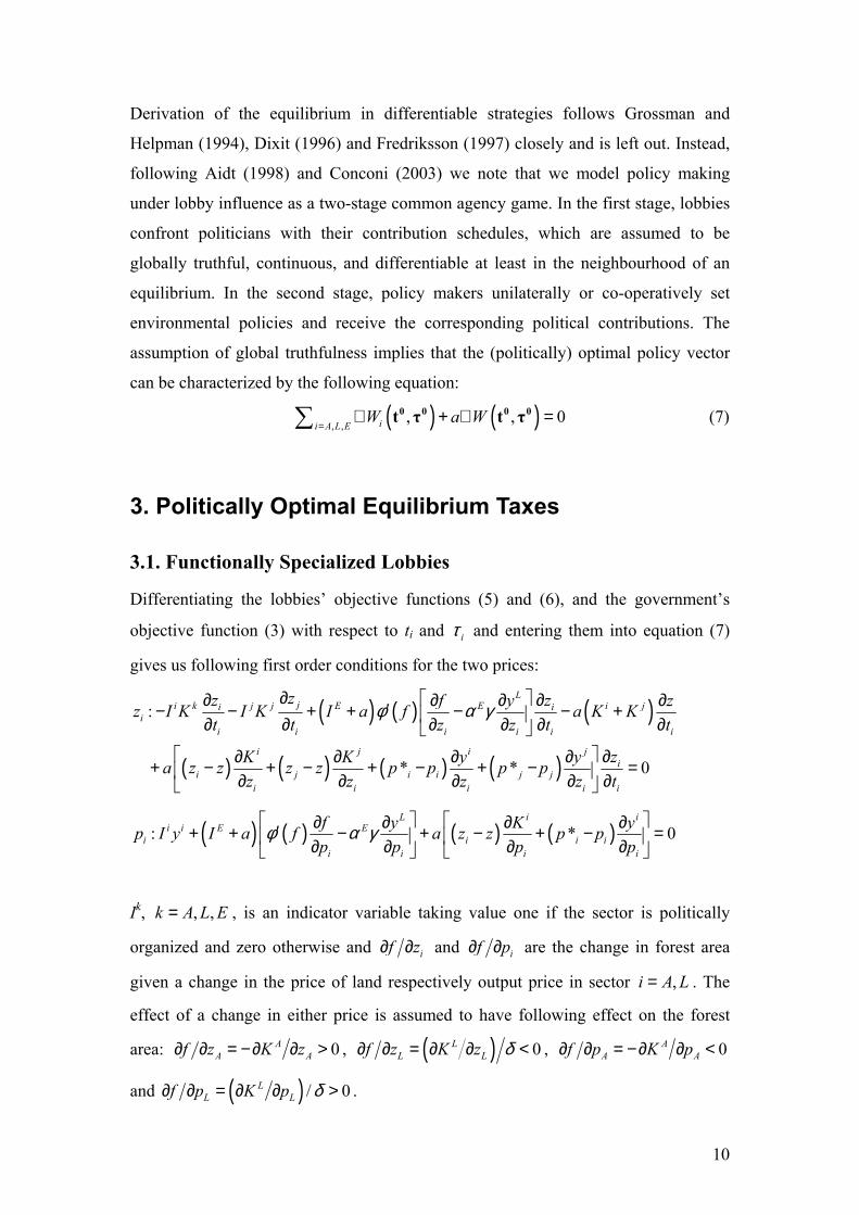
Derivation of the equilibrium in differentiable strategies follows Grossman and

Helpman (1994), Dixit (1996) and Fredriksson (1997) closely and is left out. Instead,

following Aidt (1998) and Conconi (2003) we note that we model policy making

under lobby influence as a two-stage common agency game. In the first stage, lobbies

confront politicians with their contribution schedules, which are assumed to be

globally truthful, continuous, and differentiable at least in the neighbourhood of an

equilibrium. In the second stage, policy makers unilaterally or co-operatively set

environmental policies and receive the corresponding political contributions. The

assumption of global truthfulness implies that the (politically) optimal policy vector

can be characterized by the following equation:

(7) ( ) ( ), ,, ,ii A L E

W a W=

∇ + ∇∑ 0 0 0 0t τ t τ 0=

3. Politically Optimal Equilibrium Taxes

3.1. Functionally Specialized Lobbies

Differentiating the lobbies’ objective functions (5) and (6), and the government’s

objective function (3) with respect to ti and and entering them into equation (7)

gives us following first order conditions for the two prices:

iτ

( ) ( ) ( )

( ) ( ) ( ) ( )

:

* *

Lji k j j E E i ji i

ii i i i i

i j i ji

i j i i j ji i i i i

zz z

0

i

f y zz I K I K I a f a K Kt t z z t

zK K y ya z z z z p p p pz z z z t

φ α γ∂ ∂ ∂∂ ∂′− − + + − − + ∂ ∂ ∂ ∂ ∂

∂∂ ∂ ∂ ∂+ − + − + − + − = ∂ ∂ ∂ ∂ ∂

t∂∂

( ) ( ) ( ) ( ): *L i

i i E Ei i

i i i i

f y K yp I y I a f a z z p pp p p p

φ α γ ∂ ∂ ∂ ∂′+ + − + − + − = ∂ ∂ ∂ ∂

0i

i i

Ik, , is an indicator variable taking value one if the sector is politically

organized and zero otherwise and

, ,k A L E=

if z∂ ∂ and if p∂ ∂ are the change in forest area

given a change in the price of land respectively output price in sector i A . The

effect of a change in either price is assumed to have following effect on the forest

area:

, L=

0AA AK z= −∂ ∂ >f z∂ ∂ , ( ) 0L

L Lf z K z δ∂ ∂ = ∂ ∂ < , 0f p p∂ ∂ = <AA AK−∂ ∂

and ( ) / 0LL LK p δ∂ ∂ >f p =∂ ∂ .

10

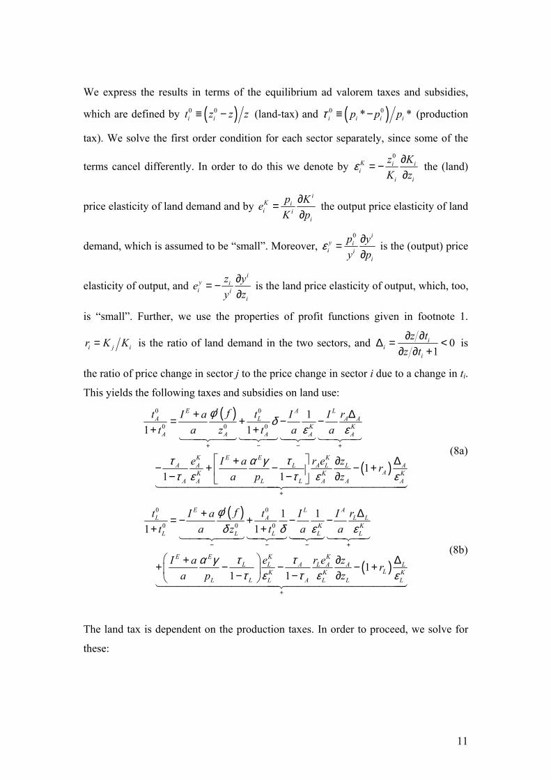
We express the results in terms of the equilibrium ad valorem taxes and subsidies,

which are defined by ( )0 0i it z z≡ − z (land-tax) and ( )0 0*i i i *ip p pτ ≡ − (production

tax). We solve the first order condition for each sector separately, since some of the

terms cancel differently. In order to do this we denote by 0

K ii

i i

z KK z

ε ∂= −∂

i the (land)

price elasticity of land demand and by i

K ii i

i

p KK p

∂=∂

e the output price elasticity of land

demand, which is assumed to be “small”. Moreover, 0 i

y ii i

i

p yy p

ε ∂=∂

is the (output) price

elasticity of output, and i

y ii i

i

z yey z

∂= −∂

is the land price elasticity of output, which, too,

is “small”. Further, we use the properties of profit functions given in footnote 1.

i jr K K= i is the ratio of land demand in the two sectors, and 01

ii

i

z tz t∂ ∂ <

∂ ∂ +∆ = is

the ratio of price change in sector j to the price change in sector i due to a change in ti.

This yields the following taxes and subsidies on land use:

( )

( )

0 0

0 0 0

11 1

11 1

E A LA L A A

K KA A A A A

K KE EA A L A L L

AA

K K KA A L L A A

ft t rI a I It a z t a a

e r e zI a ra p z

φδ

ε ε

τ τα γτ ε τ ε ε

+ − − +

+

′ ∆+= + − −+ +

∂ ∆+− + − − + − − ∂ A

(8a)

( )

( )

0 0

0 0 0

1 11 1

11 1

E L AL A L

K KL L L L L

K KE EL L A L A A

L

L

LK K K

L L L A L L

ft t rI a I It a z t a a

e r e zI a ra p z

φδ δ ε ε

τ τα γτ ε τ ε ε

− − − +

+

′ ∆+= − + − −+ +

∂ ∆++ − − − + − − ∂ L

(8b)

The land tax is dependent on the production taxes. In order to proceed, we solve for

these:

11

( )0 0

0 0

/

11 1

yE AA A

yA

yA A A A

f t eI a Ia z t a

φττ ε

+ −

− +

′ += − − − +

Aε

−

(9a)

( )0 0

0

/

11 1

yE E E LL

yL L L L L

f t eI a I a Ia p a z t a

φτ α γτ δ

+ −− +

′ + += − + − − + 0

L LyLε ε

(9b)

We start the analysis of these equations by defining as sA and sL the parts of (8a) and

(8b) that are not dependent on the land tax-cum-subsidy itself:

( ) ( ) ( )

( ) ( )

11

1 01

KE A LA A A A

A K K KA A A A A

KE EA LL L

AK KL L A A A

f r eI a I Isa z a a

r e zI a ra p z

φ δ τδε ε τ ε

δτα γ δτ ε ε

′ ∆+= − − −−

∂ ∆+ + − − + − ∂

A > (10a)

( ) ( ) ( )

( ) ( )

1

1 01 1

E L AL L

L K KL L L

KKE EL AL L A A L

LK KL L L A L L L

f rI a I Isa z a a

r ee zI a ra p z

φ δδ

δ ε εδτ τα γ δ

τ ε τ ε ε

′ ∆+= − − −

∂ ∆+ + − − − + − − ∂

K < (10b)

sA and sL have been defined as functions of δ for future use. Examining their

properties gives us the following two propositions:

Proposition 1: Given that 1

LA

L

sss

< −−

, the land-tax will be positive for the

agricultural sector and given that 1

A

A

ss

> −− Lsδ it will be negative (a subsidy) for the

logging sector.

Proof: We start by solving equations (9a) and (9b) as functions of equations (10a) and

(10b), which give us the following:

( )( )

0 1A LA

A L A L

s s st

s s s sδ− +

= −+ −

L (11a)

12

( )( )

0 1A AL

L

A L A L

s s st

s s s sδ

δ− −

=+ −

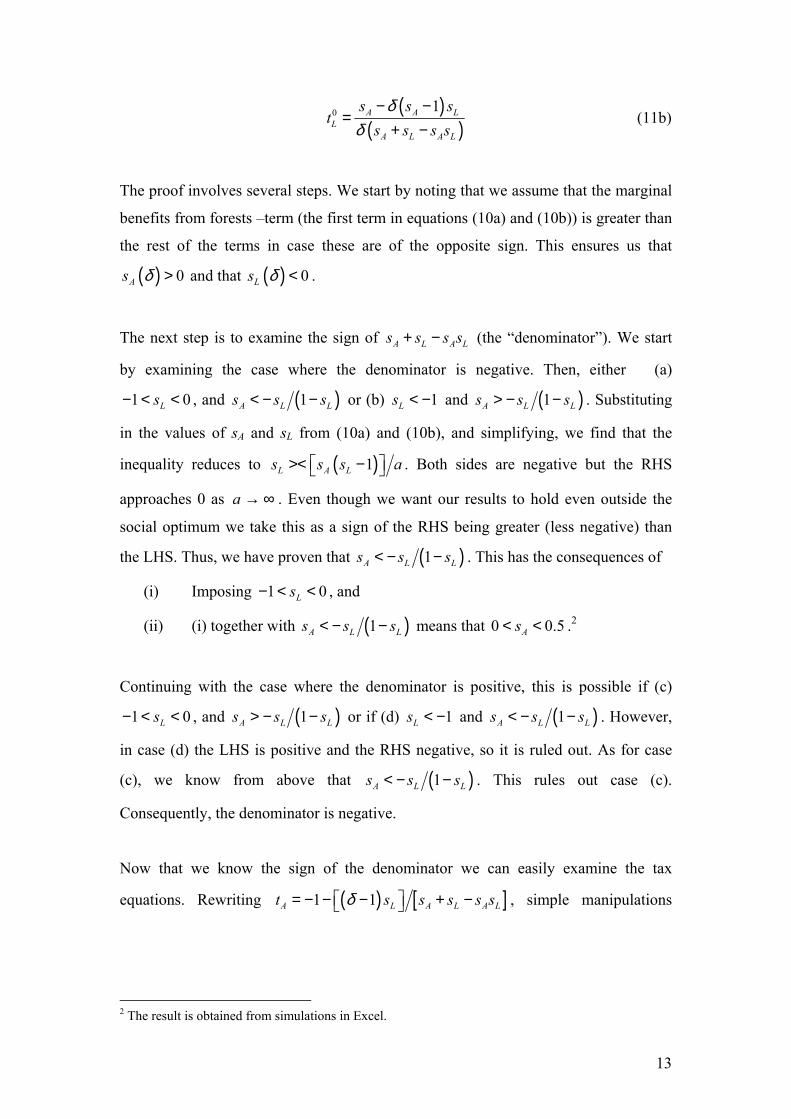
(11b)

The proof involves several steps. We start by noting that we assume that the marginal

benefits from forests –term (the first term in equations (10a) and (10b)) is greater than

the rest of the terms in case these are of the opposite sign. This ensures us that

and that . ( ) 0As δ > ( ) 0Ls δ <

The next step is to examine the sign of A L As s s s+ − L

)

(the “denominator”). We start

by examining the case where the denominator is negative. Then, either (a)

, and 1 0Ls− < < (1A Ls s s< − − L ) or (b) and 1Ls < − (1A Ls s s> − − L . Substituting

in the values of sA and sL from (10a) and (10b), and simplifying, we find that the

inequality reduces to ( )1L A Ls s s>< − a

(

. Both sides are negative but the RHS

approaches 0 as a . Even though we want our results to hold even outside the

social optimum we take this as a sign of the RHS being greater (less negative) than

the LHS. Thus, we have proven that

→ ∞

)1A Ls s s< − − L

)

. This has the consequences of

(i) Imposing − < , and 1 0Ls <

(ii) (i) together with (1A Ls s s< − − L

)

means that .0 0.5As< < 2

Continuing with the case where the denominator is positive, this is possible if (c)

, and 1 0Ls− < < (1A Ls s s> − − L ) or if (d) and 1Ls < − (1A Ls s s< − −

)

L . However,

in case (d) the LHS is positive and the RHS negative, so it is ruled out. As for case

(c), we know from above that (1A Ls s − Ls< − . This rules out case (c).

Consequently, the denominator is negative.

Now that we know the sign of the denominator we can easily examine the tax

equations. Rewriting ( ) [ ]1 1A L A L At s s sδ = − − − + − Ls s

, simple manipulations

2 The result is obtained from simulations in Excel.

13

show that this will be positive if ( )1L Ls sδ− − <

)As 1. We know that . Then,

assuming that

0 δ< <

(1A Ls s s→ − −

0>

L , we know that the inequality holds.3 Then,

1As −

.9

(iii) and At

(iv) We can delimit further ( ) ( )1 1L L A Ls s s s sδ− − < < − − L .

Rewriting ( ) ( )1 1L A A Lt s s sδ δ A Ls s = + − + −

( )

, simple manipulations show that

if 0Lt < 1A A Ls s sδ− > −

( )

. Simulations in Excel show that as long as

1A L Ls− ( )s s< − , 1A A − Ls )s s− < . As (1A Ls s s→ − − L , the closer ( )As is

to sL. Then, for most reasonable values of δ (from Excel, ), 0 0δ< ≈

(v) ( )1L A As s s sδ− < − < − L . Then we deem it safe to make our final

conclusion:

(vi) . Q.E.D. 0Lt <

Proposition 1 shows the importance of considering the connection between the two

sectors. For instance, tA would be unambiguously positive if it were not for the effect

of that drags it down. Similarly, tLsδ L would be unambiguously negative if sA did not

tend to “pull it up”. When the input market is thus interconnected, it would be wrong

not to consider the effect of the changes in the price of the common input.

We turn next to the size of the respective tax and formulate following proposition:

Proposition 2: and − < . The former implies and the latter

.

1At > 1 0Lt < ( )0 2Az z> t

( )00 Lz z< < t

Proof: From proposition 1 we know that . We prove proposition 2 by proving

that the opposite

0At >

( ) [ ]1 1A L A Lt s s s sδ = − − − − <

( ) (

1A Ls+

)

is ruled out. Simple

manipulation yields ( ) ( )1 1 1 1 2L L L L Ls s s s s− + − − − − >

1A >

Lsδ δ=− As

. From

finding (iv) in Proposition 1 we know that this is no true. Thereby, t .

3 Simulations made in Excel support the assumption.

14

Manipulation of ( ) ( )1 1L A A L A Ls s s sδ δ= + − + − < −1t s yields the condition

( ) ( )1 1 2A A Ls sδ+ − > −

( )

sδ 0Lt < for . From finding (v) in Proposition 1 and because

1A A Ls s sδ δ− < − this can be rejected. Therefore, we conclude that . 1 0Lt− < <

The latter part of the proposition is obvious from a manipulation of the definition of

the (ad valorem) tax. Q.E.D.

Examining the government’s decision in the setting of tax-cum-subsidies, we

formulate the following proposition that supports the findings of Aidt (1998):

Proposition 3: The (main) instrument to internalize the externality arising from forest

amenities is a land tax-cum-subsidy and the (main) instrument to internalize the

production externality in the logging sector is a production tax on that sector.

Proof: Proposition 3 cannot be proved directly but an examination of the tax

equations (8a), (8b), (9a) and (9b) supports it. The production externality enters the

equations (8a) and (8b) only in a “stabilizing” fashion, i.e., the externality arising

from production is subtracted from the production tax. The terms are further

multiplied by the output price elasticity of land demand, which is assumed to be

small. These terms are thus bound to be close to zero and the land tax-cum-subsidy

equations are dominated by the marginal benefits from forests –term.

Similarly, in the case of the production taxes (9a) and (9b), the externality arising

from land use is subtracted from the land-tax and multiplied by the land price

elasticity of output that is assumed to be small. Therefore, the first term in (9a) and

the second term in (9b) are bound to be close to zero and (9a) is approximately zero

and (9b) dominated by the first term measuring the disutility from logging.

The presence of lobbies does not change these findings, they just lead to a downward

pressure on the taxes from sector i and upward pressure from sector j and the

environmentalists. Q.E.D.

15

The government imposes the land tax-cum-subsidy because of three reasons: first, in

order to internalize the externality from land use, second, to raise tax revenue and

third, to stabilize the effect of production taxation. The production tax is imposed,

first, in order to internalize the production externality in the logging sector and

second, to stabilize the effect of land taxation, but not in order to raise tax revenue. In

absence of lobbying the government would use a production tax on the agricultural

sector only to adjust for the deviation from the Pigouvian land-tax rate. Finally,

similarly to Aidt (1998), all taxes, although not set to their Pigouvian levels, contain a

Pigouvian element.

Turning finally to the effect of lobbying, we formulate the following proposition:

Proposition 4: Environmentalists lobby for higher-than-Pigouvian environmental

taxes (or land use subsidy for logging) whereas the industrial sectors lobby for lower

own taxes but higher land-tax on the other sector. The overall impact of lobbying is

ambiguous.

Proof: This can be seen by examining the signs of the terms including the lobbying

parameter Ik, . The Pigouvian land tax-cum-subsidy would equal the

marginal benefits from forests (

, ,k A L E=

( )( )( ii i )if z f z K zφ′ ∂ ∂ ∂ ∂ ). The environmentalists

give more weight to the first term in both equations (8a) and (8b), thus leading to

higher-than-Pigouvian land tax-cum-subsidy in absence of other effects. The

Pigouvian production tax on sector A is zero and on sector L equal to ELpα γ . The

presence of environmentalists rises the first term in equation (9b) thus leading to a

higher production tax on logging.

Similarly, the third term in equations (8a) and (8b) is negative due to industry

lobbying by the sector being taxed, given that the sector organizes a lobby, and the

fourth term in these equations is positive, thus rising the tax. The fourth term arises

from industry j’s interest to lobby for higher land-price for sector i because this

benefits sector j by allocating more land to that sector via the price mechanism. Each

sector’s political clout depends on sector i’s (land price) elasticity of land use, and for

sector j on its share of land use (ri). The higher the elasticity of land use, the less

16

sector i’s lobbying weighs in; the higher share of land in sector j, the higher that

sector’s influence.

Finally, both industrial lobbies lobby for a lower production tax on their own sector

and do not concern themselves with the production tax on the other sector. Given that

the first term in (9a) is small, this leads to agricultural production being subsidized.

The overall effect of lobbying, with both environmental and industrial lobbies present

is however ambiguous, except in the case of equation (9a) where the environmental

lobby does not enter. Q.E.D.

3.2. Multi-purpose Lobbying and the Political Equilibrium

In this section we study how the equilibrium tax rates change if the lobbies have

multiple goals instead of a single one. The multiple goals consist not only of

maximizing each sector’s profits or the level of environmental taxation but of also

maximizing the tax-remittances coming from the government and, for the industrial

lobbies, to lobby for a greater provision of forests because of the amenities these

produce.

We do not give the explicit tax forms here since they are very similar to equations

(8a), (8b), (9a) and (9b). The difference arises from the weights that the different

terms get. It is noteworthy that because of the way we have specified our model,

multipurpose lobbying increases the weight given to the forest amenities to

b b

b B b Ba I a α

∈ ∈

+ +

∑ ∑

, where b

b BI

∈∑ equals 3 if all lobbies organize. Thus, when a

is finite and the government takes both contributions and the social welfare into

consideration in its decision-making, the provision of forests increases, i.e., the land

tax on agriculture and the subsidy on land use in logging will both be higher, and the

forest area is more bound to exceed the socially optimal level than in the previous

section where only the environmentalists lobbied for its provision. The production tax

equation does not change in a significant manner, however.

17

4. Effect of Property Rights on Levels of Taxes As noted in the introduction, the property rights regime may have a profound effect

on forest cover. In this section we examine how a change in the “property rights

parameter” δ impacts the taxes solved for in section 3. We start with some intuition on

the effect of property rights. We noted above that the land price equals the ratio of the

value of marginal product of land: ( ) ( )ii j i K j Kz z p y p y= j . It is a well-known

postulate of welfare economics that when property rights to a resource are poorly

defined, the producers produce at a point where the value of average product equals

price. Further, for a given KL, L LL

LL Kp y K p y> , i.e., average product of land is

higher than its marginal product.

In this section we assume that the land price is fixed. Then, as we examine

changes in the property rights parameter δ, which will be higher if the property rights

to forests are poorly defined and has the consequence of increasing production:

( )z t

( )( ), ,LLy pδ∂ z t 0δ∂ > , only the changes that arise through changes in tax policies

are considered. The reason for this assumption is that for L L LL L K Lp y K p y z= = to

hold, the KL in the average product function has to be greater than the last unit of land

entering into the marginal product function for the value of production to be the same.

I.e., of the given area f, under poorly defined property rights to forests a greater area

will be logged. In order not to mix the effects we then exclude the possibility of

property rights impacting on . ( )z t 4

It is important to note that we do not define the level of δ at which property rights are

“well defined” (i.e., private property rights apply and are enforced) and when they are

“poorly defined” (i.e., open access to forests). This could naturally be solved for, but

4 If we wanted to make the model more realistic we should allow the land-price, z(t), to be a function of property rights, too. This would mean that the worse the property rights to forests, the higher the land price for both sectors. This would have an effect of “allocating away” land from forests to agriculture as we “worsened” the property rights. As long as the price adjustment was not equal to the change in the property rights, the adjustment would not be full. As this complication does not give more insight to the effect of property rights it is left away and we assume constant prices. A further motivation for leaving it unconsidered is that no land just shifts its “property rights parameter” in the described fashion.

18

since we do not attempt to do this, the analysis merely shows is how the levels of

taxes and thus the society’s perception of the value of forests change with δ.

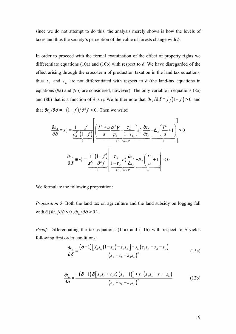
In order to proceed with the formal examination of the effect of property rights we

differentiate equations (10a) and (10b) with respect to δ. We have disregarded of the

effect arising through the cross-term of production taxation in the land tax equations,

thus Aτ and are not differentiated with respect to δ (the land-tax equations in

equations (9a) and (9b) are considered, however). The only variable in equations (8a)

and (8b) that is a function of δ is r

Lτ

i. We further note that ( )1 0Ar f fδ = − >∂ ∂ and

that ( ) 21r fδ δ− < 0fL∂ ∂ . Then we write: = −

( )/ , "small"

1 1 01 1

E E LKA L L

A LKA L L A

s zf I a Is ef a p z a

τα γδ ε τ

++ −+

∂ ∂+′ ≡ = − −∆ + > ∂ − − ∂

A

( )2

/ , "small"

11 1 01

AKL A A

L A LKL A L

fs z Is ef z a

τδ ε δ τ

+ + − −

− ∂ ∂′≡ = +∆ + < ∂ − ∂

We formulate the following proposition:

Proposition 5: Both the land tax on agriculture and the land subsidy on logging fall

with δ ( 0At δ∂ ∂ < , 0Lt δ∂ ∂ > ).

Proof: Differentiating the tax equations (11a) and (11b) with respect to δ yields

following first order conditions:

( ) ( ) (

( ))

2

1 1A L L L A L L A A LA

A L A L

s s s s s s s s s sts s s s

δδ

′ ′ − − − + − −∂ =∂ + −

(15a)

( ) ( ) (

( ))

2

1 1A L A L A A A L A LL

A L A L

s s s s s s s s s sts s s s

δ δδ

′ ′ − − + − + − −∂ =∂ + −

(12b)

19

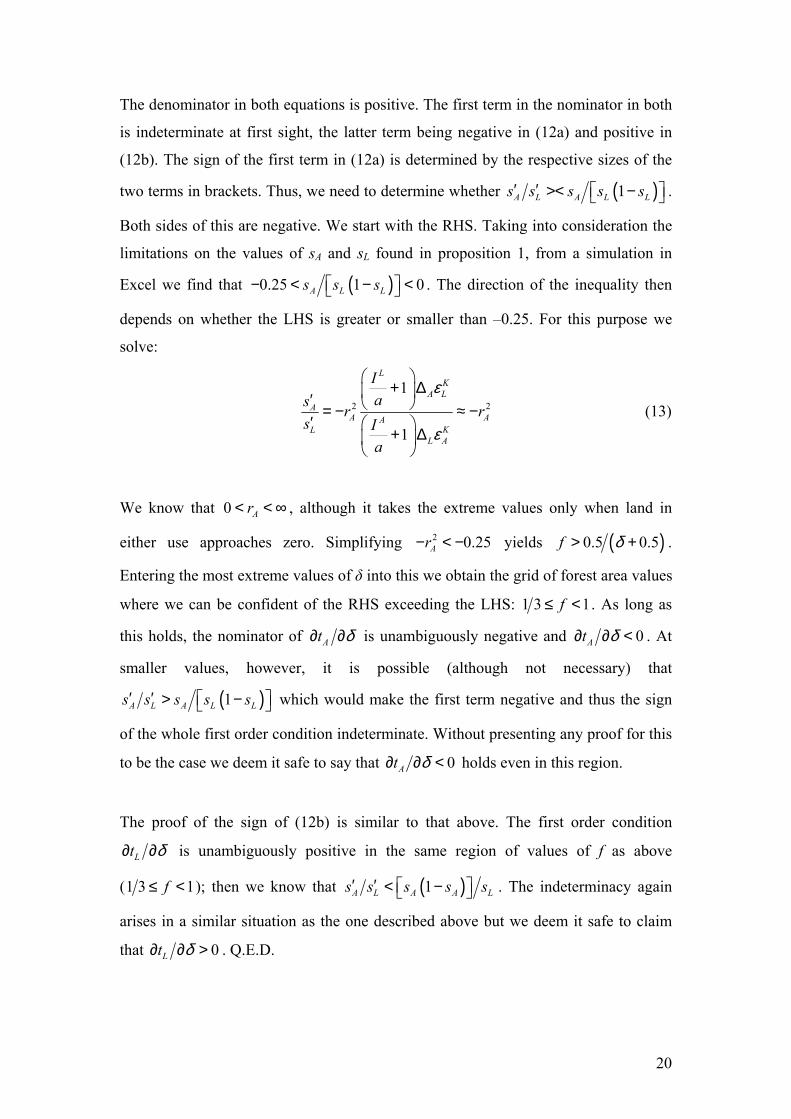
The denominator in both equations is positive. The first term in the nominator in both

is indeterminate at first sight, the latter term being negative in (12a) and positive in

(12b). The sign of the first term in (12a) is determined by the respective sizes of the

two terms in brackets. Thus, we need to determine whether ( )1A L A L Ls s s s s′ ′ >< − .

Both sides of this are negative. We start with the RHS. Taking into consideration the

limitations on the values of sA and sL found in proposition 1, from a simulation in

Excel we find that ( )0.25 1 0A L Ls s s − < − < . The direction of the inequality then

depends on whether the LHS is greater or smaller than –0.25. For this purpose we

solve:

2

1

1

LK

A LA 2

A AAKL

L A

Ias r

s Ia

ε

ε

+ ∆ ′ = − ≈ −

′ + ∆

r (13)

We know that , although it takes the extreme values only when land in

either use approaches zero. Simplifying yields

0 Ar< < ∞

2 0.25Ar− < − ( )0.5 0.5f δ> + .

Entering the most extreme values of δ into this we obtain the grid of forest area values

where we can be confident of the RHS exceeding the LHS: 1 3 1f≤ < . As long as

this holds, the nominator of At δ∂∂ is unambiguously negative and 0At δ <∂ ∂ . At

smaller values, however, it is possible (although not necessary) that

( )1L Ls −A L As s s s′ ′ > which would make the first term negative and thus the sign

of the whole first order condition indeterminate. Without presenting any proof for this

to be the case we deem it safe to say that 0δ <At∂ ∂ holds even in this region.

The proof of the sign of (12b) is similar to that above. The first order condition

Lt δ∂ ∂ is unambiguously positive in the same region of values of f as above

(1 3 1f≤ < ); then we know that ( )1A L A As s s s s′ ′ < − L . The indeterminacy again

arises in a similar situation as the one described above but we deem it safe to claim

that 0>Lt δ∂ ∂ . Q.E.D.

20

Again, the cross-effect between the two land tax-cum-subsidy schemes for the two

sectors causes indeterminacy: it makes the f.o.c of tA higher than would otherwise be

the case and lowers the f.o.c. of tL.

What is the intuition behind these first order conditions? With less-well defined

property rights to forests the government lowers both the subsidy to land use in

logging and the tax on land use in agriculture. The signs arise from the fact that the

government, instead of subsidizing forests, subsidizes land use for logging. A higher δ

leads to a perception of more land being forested and thus lowers the need for

subsidizing land use in logging. In reality, in order not to make matters worse the land

tax-cum-subsidy scheme should remain constant. As it is, the changes in the tax and

subsidy lead to more land being allocated to agriculture and less to forests.

In order to determine whether the incentives to change the production tax are as

perverted as the ones above, we formulate and prove the next proposition:

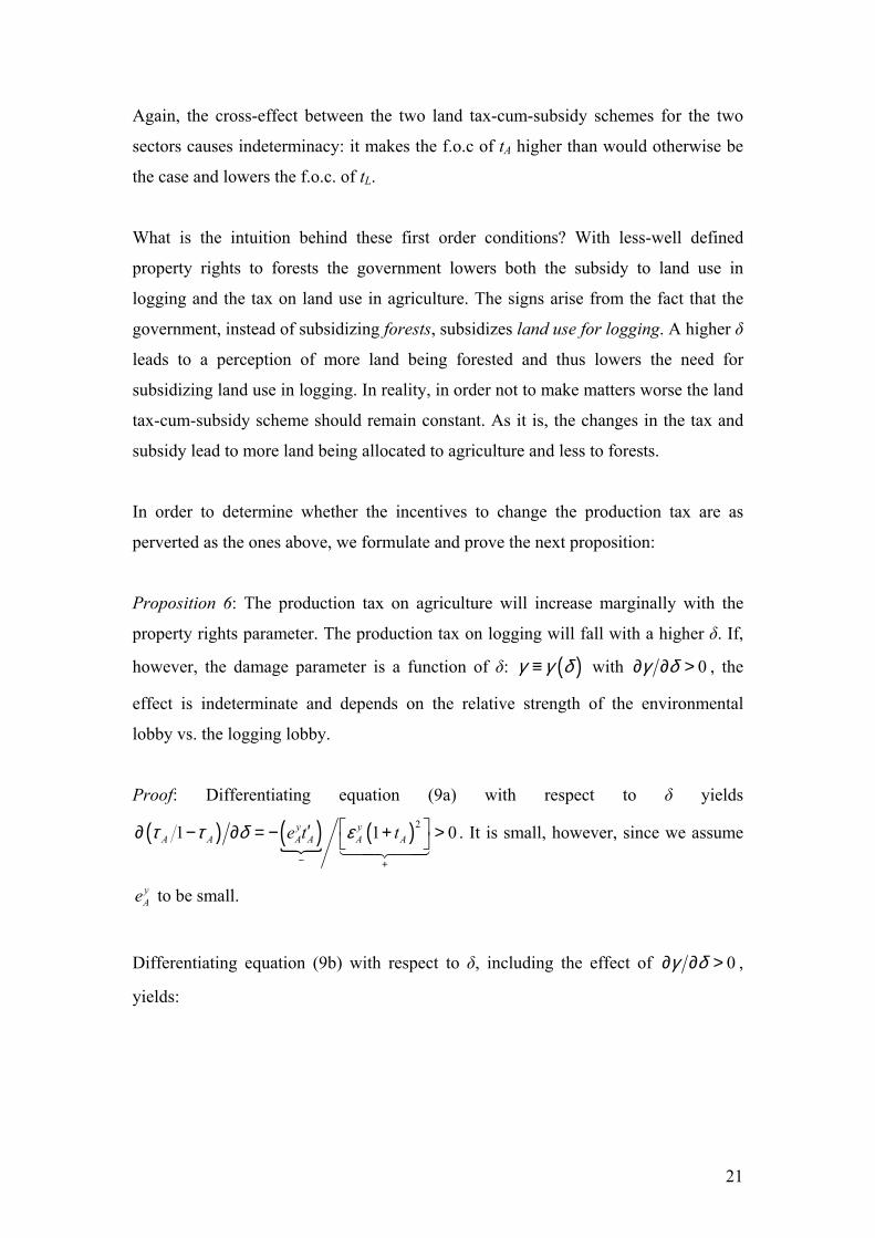
Proposition 6: The production tax on agriculture will increase marginally with the

property rights parameter. The production tax on logging will fall with a higher δ. If,

however, the damage parameter is a function of δ: ( )γ γ δ≡ with 0γ δ∂ ∂ > , the

effect is indeterminate and depends on the relative strength of the environmental

lobby vs. the logging lobby.

Proof: Differentiating equation (9a) with respect to δ yields

( ) ( ) ( )21 y yA A A A A Ae t tτ τ δ ε

− +

′∂ − ∂ = − + >

y

1 0 . It is small, however, since we assume

Ae to be small.

Differentiating equation (9b) with respect to δ, including the effect of 0γ δ >∂ ∂ ,

yields:

21

( )( )

( ) ( )

( )

2

2

/ , "small"

1

1 11 1

yL LEE L

L

yL L

y yE Ey yL L L L LL L L

L L L L L

yL

I a Ia p a

f ft e t tI a I ae ea z t a z t t

τ εα γ δτ δ

δ ε

φ φε ε εδ δ δ δ δ

ε

+−

+ −

∂∂ ′− + ∂= +∂

′ ′ ′ ∂ ∂+ ++ − + − − + ∂ ∂ + + +1

y yL

(14)

We examine two scenarios. In the first one we set 0γ δ∂ ∂ = , which, considering that

the third term in the first order condition is “small”, makes the first order condition

negative. In this case lobbying by the logging sector leads to a greater fall in the

production tax the worse the property rights are.

In the second scenario we again set 0γ δ >∂ ∂ . This means that the

environmentalists’ perception of the damage caused by logging increases in the

property rights parameter.5 Now the sign of the first order condition is dependent on

the relative strengths of the environmental and logging lobbies. For instance, if the

environmental but not the logging lobby organizes, the first order condition is

automatically positive; in the opposite case it is negative. Further, as αE increases, the

weight given to the externality increases and thereby the environmentalists clout in

setting the tax. Q.E.D.

The intuition behind proposition 6 is that in countries with poorly defined property

rights to forests, the logging industry’s production is higher and therefore the industry

has more at stake and lobbies even more intensively for a low production tax on

logging than in countries with well-defined property rights to forests. The reason why

we examined both the case where 0γ δ >∂ ∂ and where it is constant is that we

question the ability of the environmentalists to determine the nature of property rights

to forests. Therefore, we deem the case where the environmentalists do not vary their

lobbying depending on δ the more plausible.

5 How the environmentalists are able to observe such variations in δ across countries is beyond the scope of the paper.

22

The results obtained so far shed light to the possibilities of forest conservation in

countries with open access to forests. Thus, they explain why a government in a

country with less-well defined property rights to forests allocates less land to

agriculture and more to forests than would be socially optimal, and might even allow

for more agricultural land conversion (the effect from 0At δ <∂ ∂ and 0Lt δ >∂ ∂ ).6

The effect of production taxation only aggravates the situation as the logging sector

intensifies its lobbying for lower production taxation thereby increasing the area

logged even more (pL increases as production taxation falls thereby increasing

production).

Considering finally the effect of lobbying/bribes on the situation we formulate our

final proposition:

Proposition 7: When property rights to forests are poorly defined the stake of the

logging industry is greater than when they are well defined. This intensifies lobbying

by the logging lobby, which leads to a higher production of logs than in absence of

logging. If both industry lobbies organize, they do not affect the land-tax.

Proof: Starting from the latter statement, from proposition 4 we know that the effect

of lobbying on tax rates is ambiguous. An examination of the is δ∂ ∂ ’s,

shows that an organized sector j lobbies for a higher tax on sector i. However, the first

order conditions

,i A L=

is δ∂∂ do not enter the first order conditions of the tax equations

it δ∂ ∂ as such but in the ratio A Ls s′ ′ (equation (13)). If both industries organize a

lobby, their effects cancel out thus leaving it δ∂∂ intact. If, however, either industry

does not organize into a lobby, then the other sector has and impact on it∂ δ∂ . If the

sector that organizes is the logging sector, this has the impact of making the first order

conditions less steep. This would mean that more land was allocated to forests than

when both sectors organize, given the property rights. If the sector that organizes is

6 The socially optimal land allocation is naturally the one where property rights to forests are well defined and when the government puts all weight on social welfare and disregards of lobbying.

23

the agriculture, then the term serves to make the slope of the first order conditions

it δ∂ ∂ even steeper, thus allocating more land to agriculture and less to forests.

In the case of the production tax the agricultural sector does not change its lobbying

strategy with the property rights parameter. As already noted in the proof of

proposition 6, the logging sector, however, has more at stake and intensifies it’s

lobbying for a lower production tax, which is measured by the second term in

equation (14). In presence of a logging lobby, then, the production tax on logging will

be the lower the higher δ and consequently log production will be higher. Q.E.D.

To summarize, we consider the implications of our analysis to countries that manage

to enhance their property rights regimes and establish better-defined property rights to

forests. From the land tax-cum-subsidy side of the analysis this would mean

increasing the land tax on agriculture and allocating more land to forestry. This would

increase the logging industry’s stake. At the same time, if the industry would start

logging at the marginal product of land instead of the average product, this would

lower its production, decrease lobbying for production tax and increase the production

tax on logging thus contracting its production further. If the government also managed

to tackle corruption at the same time, this would lead to an even greater increase in

the production tax to logging.

5. Conclusions This paper has shown how two production-related but separate externalities impact on

the allocation of land to forestry and agriculture. It has shown that if two sectors use a

common factor of production that is in short supply, then taxation of one sector not

only has an impact on that sector but also on the other. Further, it has been shown that

given that the government has two different tax instruments at its disposal, it can and

does use one tax instrument to compensate for inefficiencies in the use of another,

albeit these terms tend to be small, possibly even negligible.

In presence of such interdependency between the two sectors the effect of functionally

specialized lobbying on the land tax-cum-subsidy rates has been shown to be

24

ambiguous. The sector being taxed lobbies for a lower tax on its land use but the other

sector lobbies for a higher tax. Which of these effects takes overhand is impossible to

determine, especially as a third “force”, the environmentalists, also lobby for higher

taxes (or subsidies). However, in the case of a production tax, since the production of

the two goods is not related in any way, each industry lobby lobbies for lower

production tax (or a subsidy) for itself and ignores the other sector.

Lobbies with multiple goals have the effect of increasing the provision of forests for

amenities. They also lobby for tax revenue besides their own profit motivation. The

inclusion of lobbies with multiple goals does not change the conclusions of the rest of

the paper.

Finally, we studied the effect of property rights on forests. We were able to show that

the property rights regime influences government’s perception of the forest area at

least under the present specification. Thus, our findings concerning the size of the

land-tax show that we have been able to find at least one variable that explains the

disappearance of forests from countries with poorly defined property rights to forests.

Governments in countries with bad property rights regimes will tend to perceive the

forest area, and thereby the provision of amenities by forests as greater than it actually

is, consequently lowering the subsidy to forestry; subsidy that is needed in order to

internalize an otherwise under priced externality. Further, corruptible governments

tend to impose lower production taxation on logging sector, which, besides is logging

at the average product of land rather than marginal product, thus aggravating the

problem further.

As mentioned, we suspect that our analysis is dependent on the specification of the

model, however. Whether we would obtain similar results also in the case where the

government were to subsidize forest owners for their ownership of forests instead of

loggers for land use has not been studied. On the other hand, it is possible, for

instance, that it is impossible to subsidize forest owners if the government itself is the

owner of all forestland. Then policies that follow the ones delineated in this paper

may be the only ones available.

25

References: Aidt, Toke S. "Political Internalization of Economic Externalities and Environmental

Policy." Journal of Public Economics, 1998, 69(1), pp. 1-16.

____. "The Rise of Environmentalism, Pollution Taxes and Intra-Industry Trade,"

Cambridge, UK: University of Cambridge, 2000.

Bernheim, B. Douglas and Whinston, Michael D. "Menu Auctions, Resource

Allocation, and Economic Influence." The Quarterly Journal of Economics, 1986,

101(1), pp. 1-32.

Chichilnisky, Graciela. "North-South Trade and the Global Environment." The

American Economic Review, 1994, 84(4), pp. 851-74.

Conconi, Paola. "Green Lobbies and Transboundary Pollution in Large Open

Economies." Journal of International Economics, 2003, 59(2), pp. 399-422.

Dixit, Avinash. "Special-Interest Lobbying And Endogenous Commodity Taxation."

Eastern Economic Journal, 1996, 22(4), pp. 375-288.

Eerola, Essi. "Forest Conservation - Too Much or Too Little? A Political Economy

Model," Helsinki: Department of Economics, 2003, 21-43.

Ehui, Simeon K. and Hertel, Thomas W. "Deforestation and Agricultural

Productivity in the Cöte D'Ivoire." American Journal of Agricultural Economics,

1989, 71(3), pp. 703-11.

Ehui, Simeon K.; Hertel, Thomas W. and Preckel, Paul V. "Forest Resource

Depletion, Soil Dynamics, and Agricultural Productivity in the Tropics." Journal of

Environmental Economics and Management, 1990, 18, pp. 136-54.

Fredriksson, Per G. "The Political Economy of Pollution Taxes in a Small Open

Economy." Journal of Environmental Economics and Management, 1997, 33, pp. 44-

58.

____. "The Political Economy of Trade Liberalization and Environmental Policy."

Southern Economic Journal, 1999, 65(3), pp. 513-25.

Fredriksson, Per G. and Mani, Muthukumara. "Trade Integration and Political

Turbulence: Environmental Policy Consequences." Mimeo, 2003.

Fredriksson, Per G. and Svensson, Jakob. "Political Instability, Corruption and

Policy Formation: The Case of Environmental Policy." Journal of Public Economics,

2003.

26

27

Grossman, Gene M. and Helpman, Elhanan. "Protection for Sale." The American

Economic Review, 1994, 84(4), pp. 833-50.

Olson, Mancur. The Logic of Collective Action. Cambridge: Harvard University

Press, 1965.

Schleich, Joachim. "Environmental Quality with Endogenous Domestic and Trade

Policies." European Journal of Political Economy, 1999, 15, pp. 53-71.