politecnico di milano · i would like to thank politecnico di milano for the facilities and support...
TRANSCRIPT

POLITECNICO DI MILANO FACULTY OF ENGINEERING
DEPARTMENT OF MECHANICAL ENGINEERING
DYNAMIC ANALYSIS OF A PLANAR 2-DoF MANIPULATOR DRIVEN BY PNEUMATIC ACTUATORS
Supervisors:
1. Eng. Hermes Giberti, and
2. Ing. Simone Cinquemani
Thesis By:
Mhretie Molalign M.
Academic year 2009/2010

Abstract
In recent years, parallel manipulators have become increasingly popular in industries,
especially, in the field of machine tools handling and, pick and place operations. In this thesis
work, a planar 2-degree-of-freedom (DoF) parallel-kinematic-mechanism (PKM) manipulator,
which is actuated by a pair of pneumatic drives is proposed. A full kinematic analysis of the
manipulator is discussed in reference with a desired trajectory and motion law. In this analysis
it is shown that the inverse and forward kinematics can be described in closed form; the
velocity equation, singularity, and workspace of the manipulator are presented. Furthermore,
the inverse dynamics analysis of the PKM manipulator is investigated employing the Newton-
Euler approach, which targets on getting the desired driving force that should be applied at the
joints by the actuators. After determining the drive forces, a model of pneumatic actuator is
designed, which consists of models for a standard FESTO DGP/DGPL 32 linear actuator and
for a 5/3 MYPE 1/8 proportional valve. The main work for analysis of the proposed planar
manipulator is done in a Matlab/Simulink environment. In addition, a 3D physical model of
the PKM manipulator which is created in a Solidworks graphic interface and then translated
into a Simulink/Simmechanics environment has been used in both the kinematic and dynamic
analysis stages. A numerical simulation of the manipulator is done based on the models
created and the desired trajectory and law of motion chosen. Primary results obtained from
this simulation are discussed, giving particular attention to the position error. And finally, an
appropriate control strategy is designed meant to reduce the resulting error in position of the
end-effector. At the end, a comprehensive conclusion of the entire work is presented and
necessary recommendations are forwarded.

Acknowledgement
I am heartily thankful to my supervisors, Eng Hermes Giberti and Ing Simone Cinquemani,
whose encouragement, guidance and support from the initial to the final level enabled me to
develop an understanding of the subject. I would like to thank Politecnico di Milano for the
facilities and support I gained from, in number of ways. I am very grateful to my family and
dear friends for the encouragement and huge assistance I have been getting from you.
Lastly, I offer my regards and blessings to all of those who supported me in any respect during
the completion of the work.
Molalign Mhretie

Master’s Thesis 2010 Mhretie Molalign M.
1
CONTENTS
LIST OF FIGURES .......................................................................................................... I
NOMENCLATURES & ABBREVIATIONS .................................................................. III
CHAPTER ONE ........................................................................................................... - 1 -
1. INTRODUCTION .................................................................................................. - 1 -
1.1. BACKGROUND AND MOTIVATION .............................................................................. - 1 -
CHAPTER TWO .......................................................................................................... - 3 -
2. LITERATURE REVIEW ....................................................................................... - 3 -
2.1. PARALLEL MANIPULATOR DESIGN ............................................................................. - 3 -
2.2. ROBOTS MECHANISMS AND THEIR CLASSIFICATION ................................................... - 4 -
2.2.1. Joint Primitives and Serial Linkages ................................................................ - 4 -
2.2.2. Robot Components ............................................................................................ - 5 -
2.2.3. Robotic Systems ................................................................................................ - 6 -
2.3. PARALLEL MANIPULATOR ......................................................................................... - 6 -
2.4. PNEUMATIC DRIVES ................................................................................................... - 7 -
2.4.1. Pneumatic Actuators ........................................................................................ - 7 -
2.4.2. Pneumatic Systems ........................................................................................... - 8 -
2.4.3. Pneumatic Drives Characteristics .................................................................... - 8 -
2.4.4. Pneumatic Valves ............................................................................................. - 9 -
2.5. SOLID WORK MODELING ............................................................................................. - 9 -
CHAPTER THREE .................................................................................................... - 10 -
3. KINEMATIC ANALYSIS .................................................................................... - 10 -
3.1. KINEMATIC MECHANISM DESCRIPTION ..................................................................... - 10 -
3.2. WORKSPACE OF PKM MANIPULATOR ..................................................................... - 11 -
3.3. INVERSE KINEMATIC PROBLEM ............................................................................... - 12 -
3.3.1. Position Analysis ............................................................................................ - 13 -
3.3.2. The Jacobian Matrix ....................................................................................... - 13 -
3.3.3. Velocity and Acceleration Analysis ................................................................ - 14 -
3.4. DIRECT KINEMATIC PROBLEM ................................................................................ - 14 -
3.4.1. Direct analysis for position ............................................................................ - 14 -
3.4.2. Direct analysis for velocity and acceleration ................................................. - 15 -
3.5. SINGULARITY CONDITIONS ...................................................................................... - 15 -
3.5.1. The first kind of singularity ............................................................................. - 16 -
3.5.2. The second kind of singularity ........................................................................ - 16 -

Master’s Thesis 2010 Mhretie Molalign M.
2
3.5.3. The third kind of singularity ............................................................................ - 16 -
3.6. SOLIDWORKS MODELING .......................................................................................... - 18 -
3.7. NUMERICAL SIMULATION FOR THE INVERSE KINEMATIC ANALYSIS........................ - 20 -
3.7.1. Description of sections in Simulink model ...................................................... - 20 -
3.7.2. Results and discussions ................................................................................... - 22 -
CHAPTER FOUR ............................................................................................................ - 25 -
4. DYNAMIC MODELING AND ANALYSIS ......................................................... - 25 -
4.1. DYNAMIC ANALYSIS APPROACHES ................................................................................... - 25 -
4.1.1. The Newton-Euler approach ........................................................................... - 25 -
4.1.2. Lagrangian approach...................................................................................... - 26 -
4.2. INVERSE DYNAMICS ANALYSIS THROUGH THE NEWTON-EULER APPROACH............................... - 26 -
4.2.1. The Newton-Euler approach ........................................................................... - 28 -
4.3. PNEUMATIC SERVO SYSTEM MODELING ........................................................................... - 31 -
4.3.1. Pneumatic Actuators: Modeling ..................................................................... - 31 -
4.3.2. Pneumatic Actuators: The Control Strategies: .............................................. - 31 -
4.3.3. The Dynamic Model ....................................................................................... - 31 -
4.4. SIMULATION RESULTS AND DISCUSSION ............................................................................ - 35 -
4.4.1. Thermal and physical characteristics of the pneumatic drive ........................ - 35 -
4.4.2. Simulink model of pneumatic system ............................................................. - 36 -
CHAPTER FIVE .............................................................................................................. - 37 -
5. CONTROL STRATEGIES .................................................................................. - 37 -
5.1. A REVIEW OF CONTROL STRATEGIES ................................................................................. - 37 -
5.1.1. PID Controller .................................................................................................. - 38 -
5.2. PID CONTROLLER DESIGN AND TUNING ........................................................................... - 38 -
5.2.1. Position Control .............................................................................................. - 39 -
CONCLUSIONS .............................................................................................................. - 40 -
APPENDIX A ................................................................................................................. - 41 -
1. PART I - PROGRAM DETAILS ................................................................................... - 41 -
1. PART II –SIMULINK BLOCKS DETAIL ........................................................................ - 54 -
REFERENCES ................................................................................................................. - 58 -

Master’s Thesis 2010 Mhretie Molalign M.
i
List of Figures
Figure 2.1 Types of primitive connections...............................................................................................4
Figure 2.2 A typical robot/ manipulator functional system ………………………………………….....6
Figure 2.3 The two fundamental types of pneumatic actuators .. ………………..........………………..7
Figure 2.4 Pneumatic power supply system ………………..……………………………………….. ...8
Figure 2.5 A 5-port-3-way servo valve .... …………………………………………………………. .....9
Figure 3.1 Kinematic description of the PKM manipulator.. ………………….……………………...11
Figure 3.2 Workspace envelop for a 2 DoF planar PKM manipulator.. …………………..…………..12
Figure 3.3 Singularity configuration of a PKM 2 DoF manipulator.. …………………….………......17
Figure 3.4 Singularity configuration of a PKM 2 DoF manipulator .. ………………….………….....17
Figure 3.5 Singularity configuration of a PKM 2 DoF manipulator .. …………….……………….....17
Figure 3.6 A 3D physical model of the complete PKM manipulator created with Solidworks….…...18
Figure 3.7 Solidworks individual component model for the PKM .. …………….……………….......19
Figure 3.8 A complete model of the PKM manipulator on a Simulink environment….……………...20
Figure 3.9 Inverse Kinematic Analysis (IKA):- Simulink based model.. ……………….……………21
Figure 3.10 Model of PKM Manipulator in a SimMechanics interface ……………….……………..22
Figure 3.11 Model in Simmechanics with desired motion as an input for kinematic analysis …….…22
Figure 3.12 Desired Trajectory.... ……….……………………...…………………………………….23
Figure 3.13 Desired motion law (A symmetric Constant Acceleration Law).. ……….……………...23
Figure 3.14 Desired motion law of the end effector.. ………….…………………..............................24
Figure 3.15 Desired/Reference motion law: Joint space…….………………………..........................24

Master’s Thesis 2010 Mhretie Molalign M.
ii
Figure 4.1 Position analysis for a single leg of the PKM manipulator .. ……….…………………….26
Figure 4.2 Schematic of a Pneumatic Drive System.... …………..…………………...………………32
Figure 4.3 Pneumatic drive and mechanical subsystem scheme.. ……………..………………...........33
Figure 4.4 Complete dynamic model of the PKM manipulator built in Matlab/Simulink ....................34
Figure 4.5 Detailed Simulink model of a pneumatic actuator ……………...………………................36
Figure 5.1 PID controller block diagram …………………………..…...……………………………..38
Figure 5.2 PID controller Block in Simulink library .............................................................................39

Master’s Thesis 2010 Mhretie Molalign M.
iii
Nomenclatures & abbreviations
L1 –length of legs 1 and 2
L2 –distance between sliders
L – actuator‟s maximum stroke
m –mass of each leg
ms –mass of each slider
ma –mass of moving parts in each actuator
M –mass of payload
P(x, y) – vector of position of the end-effector
Q(q1, q2) – vector of position of the joints
–angular speed
–angular acceleration
–Lagrange multiplier
Ji –moment of inertia of the ith
leg about joint point
Ps –supply pressure
Pe –exhaust pressure
Patm –atmospheric pressure
P0 –initial pressure in cylinder chambers
P1, P2 –pressure inside chamber 1 and 2, respectively
–change in pressure of air in chamber 1 and 2
Ts –supply air temperature
Te –exhaust air temperature
Tc –air temperature inside the chambers
Ap –piston cross-sectional area
V1, V2 –volume of air inside chamber 1 and 2, respectively
V10, V20 –dead-volume of air inside chamber 1 and 2, respectively
u –servo valve command signal
y –piston displacement
qm –mass flow rate of air
CP –constant pressure specific heat of air
CV –constant volume specific heat of air

Master’s Thesis 2010 Mhretie Molalign M.
iv
K=1.4 –heat ratio
R=287 [m.K1] –gas constant
B=65 [Nsm-1
] –viscous friction coefficient of air
Cd=0.8 –valve discharge coefficient
K –total kinetic energy
U –total potential energy
g –gravitational acceleration
FB –vector of reaction forces on the legs at the joints
FP –vector of reaction forces on the legs at the end-effector
Fext –vector of external forces acting on the end-effector
Mext –vector of external moments acting on the end-effector
KP –proportional gain of controller
KI –integral gain of controller
KD –derivative gain of controller
Abbreviations
PKM –Parallel Kinematic Mechanism
DoF –Degree of Freedom
PRRRP –Prismatic _Revolute _Revolute _ Revolute_ Prismatic type
joint
IKA –Inverse Kinematic Analysis
DKA –Direct Kinematic Analysis
IDA –Inverse Dynamic Analysis
ODE –Ordinary Differential Equations
PID –Proportional _ Integral _ Derivative controller

Master’s Thesis 2010 Mhretie Molalign M.
- 1 -
Chapter One
1. Introduction
1.1. Background and Motivation
Robotics is a relatively young field of modern technology that crosses traditional engineering
boundaries. Understanding the complexity of robots and their applications requires knowledge
of mechanical engineering, electrical engineering, systems and industrial engineering,
computer science, economics, and mathematics. New disciplines of engineering, such as
manufacturing engineering, applications engineering, and knowledge engineering have
emerged to deal with the complexity of the field of robotics and factory automation. Robots
can be classified as industrial robot manipulators, mobile robots, and other autonomous
mechanical systems.
The term robot was first introduced into our vocabulary by the Czech playwright Karel Capek
in his 1920 play Rossum‟s Universal Robots, the word robota being the Czech word for
work.[24] Since then the term has been applied to a great variety of mechanical devices, such
as teleoperators, underwater vehicles, autonomous land rovers, etc. Virtually anything that
operates with some degree of autonomy, usually under computer control, has at some point
been called a robot. In this text the term robot will mean a computer controlled industrial
manipulator.
This Thesis work is concerned with Parallel Kinematic Mechanism (PKM) type industrial
robot manipulator driven by pneumatic actuators, which covers the kinematics and dynamics
analysis of the PKM , motion planning and control of the manipulator under different desired
trajectories.
A parallel manipulator consists of a moving platform and a fixed base, connected by several
linkages (also called legs). As PKM are used for more difficult tasks, control requirements
increase in complexity to meet these demands. The implementation for PKMs often differs

Master’s Thesis 2010 Mhretie Molalign M.
- 2 -
from their serial counterparts, and the dual relationship between serial and parallel
manipulators often means one technique which is simple to implement on serial manipulators
is difficult for PKMs (and vice versa). Because parallel manipulators result in a loss of full
constraint at singular configurations, any control applied to a parallel manipulator must avoid
such configurations. The manipulator is usually limited to a subset of the usable workspace
since the required actuator torques will approach infinity as the manipulator approaches a
singular configuration. Thus, some method must be in place to ensure that the manipulators
avoid those configurations.
Parallel robots have many advantages comparing to the serial robots, such as high flexibility,
high stiffness, and high accuracy. To achieve a higher accuracy the static and dynamic
behavior must be better understood. The problems concerning kinematics and dynamics of
parallel robots are as a rule more complicated than those of serial one.

Master’s Thesis 2010 Mhretie Molalign M.
- 3 -
Chapter Two
2. Literature Review
2.1. Parallel manipulator Design
The conceptual design of PKM manipulators can be dated back to the time when Gough
established the basic principles of a manipulator with a closed-loop kinematic structure
(Gough, 1956), that can generate specified position and orientation of a moving platform so as
to test tire wear and tear. Stewart designed a platform manipulator for use as an aircraft
simulator in 1965 (Stewart, 1965). In 1978, Hunt (1978) made a systematic study of
manipulators with parallel kinematics, in which the planar 3-RPS parallel manipulator is a
typical one. Since then, parallel manipulators have been studied extensively by numerous
researchers.[1]
The most studied parallel manipulators are those with 6 Degree of Freedoms (DoFs). These
parallel manipulators possess the advantages of high stiffness, low inertia, and large payload
capacity. However, they suffer the problems of relatively small useful workspace and design
difficulties (Merlet, 2000). Furthermore, their direct kinematics pose a very difficult problem;
however the same problem of parallel manipulators with 2 and 3 DoFs can be described in
closed form (Liu, 2001. Moreover, for a parallel manipulator with 2 and 3 DoFs, the
singularities can always be identified readily. For such reasons, parallel manipulators with,
especially 2 and 3 DoFs, have increasingly attracted more and more researchers‟ attention with
respect to industrial applications (Tonshoff et al., 1999; Siciliano, 1999; Tsai and Stamper,
1996; Ceccarelli, 1997; Liu et al., 2001). In these designs, parallel manipulators with three
translational DoFs have been playing important roles in the industrial applications (Tsai and
Stamper, 1996; Clavel, 1988; Hervé, 1992; Kim and Tsai, 2002; Zhao and Huang, 2000;
Carricato and Parenti-Castelli, 2001; Kong and Gosselin, 2002), especially, the DELTA robot
(Clavel, 1988), which is evident from the fact that the design of the DELTA robot is covered
by a family of 36 patents (Bonev, 2001). Tsai‟s manipulator (Tsai and Stamper, 1996), in
which each of the three legs consists of a parallelogram, is the first design to solve the problem
of UU chain. A 3-translational-DoF parallel manipulator, Star, was designed by Hervé based
on group theory (Hervé, 1992). Such parallel manipulators have wide applications in the

Master’s Thesis 2010 Mhretie Molalign M.
- 4 -
industrial world, e.g., pick-and-place application, parallel kinematics machines, and medical
devices.
The existing planar 2-DoF parallel manipulators (Asada and Kanade, 1983; McCloy, 1990;
Gao et al., 1998) are the well-known five-bar mechanism with prismatic actuators or revolute
actuators. In the case of the manipulator with revolute actuators, the mechanism consists of
five revolute pairs and the two joints fixed to the base are actuated. In the case of the
manipulator with prismatic actuators, the mechanism consists of three revolute pairs and two
prismatic joints and the prismatic joints are actuated. The output of the manipulator is the
translational motion of a point on the end-effector, i.e., the orientation of the end-effector is
also changed correspondingly.
2.2. Robots mechanisms and their classification
A robot is a machine capable of physical motion for interacting with the environment.
Physical interactions include manipulation, locomotion, and any other tasks changing the
state of the environment or the state of the robot relative to the environment. A robot has some
form of mechanisms for performing a class of tasks. A rich variety of robot mechanisms has
been developed in the last few decades.
2.2.1. Joint Primitives and Serial Linkages
A robot mechanism is a multi-body system with the multiple bodies connected together. We begin by
treating each body as rigid, ignoring elasticity and any deformations caused by large load conditions.
Each rigid body involved in a robot mechanism is called a link, and a combination of links is referred
to as a linkage. In describing a linkage it is fundamental to represent how a pair of links is connected to
each other. There are two types of primitive connections between a pair of links, as shown in Figure
2.1, below. The first is a Prismatic joint where the pair of links makes a translational displacement
along a fixed axis. In other words, one link slides on the other along a straight line. Therefore, it is also
called a sliding joint. The second type of primitive joint is a Revolute joint where a pair of links rotates
about a fixed axis. This type of joint is often referred to as a hinge, articulated, or rotational joint.
a) Prismatic joint b) Revolute joint
Figure 2.1 Types of primitive connections.

Master’s Thesis 2010 Mhretie Molalign M.
- 5 -
Combining these two types of primitive joints, one can create many useful mechanisms for
robot manipulation and locomotion. These two types of primitive joints are simple to build
and are well grounded in engineering design. Most of the robots that have been built so far are
combinations of only these two types.
2.2.2. Robot Components
A particular kind of robot, whether Humanoid or industrial manipulator, consists of the
following fundamental components.
Body : the main part of the robot that helps the transformation of motion, torque or forces.
In most cases, it refers to the linkages and their mechanisms
Effectors: This are the last components to receive motion and enables a robot perform the
desired task by interacting with the external environments. The effectors maybe of various
types, the four most common ones are:
1. Impactive: – jaws or claws which physically grasp by direct impact upon the object.
2. Ingressive: – pins, needles or hackles which physically penetrate the surface of the
object (used in textile, carbon and glass fiber handling).
3. Astrictive: – suction forces applied to the objects surface (whether by vacuum,
magneto– or electro adhesion).
4. Contigutive: – requiring direct contact for adhesion to take place (such as glue, surface
tension or freezing).
Actuators: An actuator or drive is a source of motion for a robot to perform its task. It can
be of linear type(Cylinders) or rotary type(e.g. Motors). Commonly they are classified
based on the kind of medium used for energy transmission., such as Electrical, Hydraulic,
Pneumatic and Internal Combustion (IC) hybrids.
Sensors: sensors are those components that helps to acquire a feedback action by
interaction with the surrounding of the robot.
Controller: The controllers are used to maintain the robot precision, stability, linearity and
manageability within a desired appropriate limits.

Master’s Thesis 2010 Mhretie Molalign M.
- 6 -
2.2.3. Robotic Systems
A robot manipulator should be viewed as more than just a series of mechanical linkages. The
mechanical arm is just one component in an overall Robotic System, illustrated in Figure 2.2,
which consists of the arm, external power source, end-of-arm tooling, external and internal
sensors, computer interface, and control computer. Even the programmed software should be
considered as an integral part of the overall system, since the manner in which the robot is
programmed and controlled can have a major impact on its performance and subsequent range
of applications.
Figure 2.2 A typical robot/ manipulator functional system
2.3. Parallel Manipulator
A parallel manipulator is one in which some subset of the links form a closed chain. More
specifically, a parallel manipulator has two or more independent kinematic chains connecting
the base to the end-effector. The closed chain kinematics of parallel robots can result in
greater structural rigidity, and hence greater accuracy, than open chain robots. The kinematic
description of parallel robots is fundamentally different from that of serial link robots and
therefore requires different methods of analysis. [22]
A parallel mechanism is one of the most active areas of current mechatronics and robotics
research. Since it is promising to have those supplementary features that serial mechanisms is
in lack of such as high rigidity, high stiffness, high accuracy, high speed, high acceleration
and high payload. However they are much more complicated than the serial mechanisms due
the presence of closed loop constraints. And our understanding of them is far behind that of
serial mechanisms, which have been extensively studied. [23]
Power
supply
Mechanical
arm
Computer
controller
End-of-arm
tooling
Sensors
Program
storage
Input
device

Master’s Thesis 2010 Mhretie Molalign M.
- 7 -
2.4. Pneumatic drives
What is an actuator? An actuator is a mechanical device used for moving or controlling
something (in this case manipulators). Generally, based the medium used to transfer energy,
actuators/drive are classified as:
• Electric Motors and Drives
• Hydraulic Drives
• Pneumatic Drives
• Internal Combustion hybrids
2.4.1. Pneumatic Actuators
Most of the earlier pneumatic control systems were used in the process control industries,
where the low pressure air of the order 7-bar was easily obtainable and give sufficiently fast
response. Pneumatic systems are extensively used in the automation of production machinery
and in the field of automatic controllers. For instance, pneumatic circuits that convert the
energy of compressed air into mechanical energy enjoy wide usage, and various types of
pneumatic controllers are found in industry. Certain performance characteristics such as fuel
consumption, dynamic response and output stiffness can be compared for general types of
pneumatic actuators, such as piston-cylinder and rotary types. Figure below shows the two
types of pneumatic actuators [30] The pneumatic actuator has most often been of the piston
cylinder type because of its low cost and simplicity . The pneumatic power is converted to
straight line reciprocating and rotary motions by pneumatic cylinders and pneumatic motors.
The pneumatic position servo systems are used in numerous applications because of their
ability to position loads with high dynamic response and to augment the force required moving
the loads. Pneumatic systems are also very reliable. [30]
a) Double acting linear pneumatic actuator. b) Vane rotary pneumatic actuator.
Figure 2.3 The two fundamental types of pneumatic actuators

Master’s Thesis 2010 Mhretie Molalign M.
- 8 -
2.4.2. Pneumatic Systems
Pneumatic systems are designed to move loads by controlling pressurized air in distribution
lines and pistons with mechanical or electronic valves.
Air under pressure possesses energy which can be released to do useful work.
Some examples of pneumatic systems are: dentist‟s drill, pneumatic road drill, automated
production systems.
Figure 2.4 Pneumatic power supply system
2.4.3. Pneumatic Drives Characteristics
Many of the same principles as hydraulics except working fluid is compressed air
Compressed air widely available and environmentally friendly,
Piping installation and maintenance is easy
Explosion proof construction
Major disadvantage is compressibility of air, leading to low power densities and poor
control properties (usually on/off)
Pneumatic systems are suitable for light and medium loads (30N-20kN) with temperature -
40 to 200 degrees Celsius
In general pneumatic systems have the following key merits
Low cost and easy to install
Clean and easy to maintain
Low power densities
Only on/off or inaccurate control necessary

Master’s Thesis 2010 Mhretie Molalign M.
- 9 -
2.4.4. Pneumatic Valves
Pneumatic valve is a component placed in between the reservoir and the cylinder for the
purpose of regulation the flow of air. It regulates the air flow to and from the cylinder
according to an appropriate command given to it as an electrical signal. The two most
common types electromechanical servo valves are the three port –two way (3-2) and the five
port- three way (5-3) valves. Figure 2.5 shows the very simple type of a 5-3 servo valve
connected to a double action, single rod cylinder.
Figure 2.5 A 5-port-3-way servo valve
2.5. Solid work modeling
SolidWorks is a Parasolid-based solid modeler, and utilizes a parametric feature-based
approach to create models and assemblies. It is capable of carrying out numerous tasks
ranging from simple components physical modeling up to simulation, motion study and
sustainability analysis of a more complex assembly. However, in this thesis work the use of
Solid work is limited, it will be implemented for creating a 3D physical model of the
manipulator, which principally can be translated into Matlab/Simulink-SimMechanics
interface. The general step used in the modeling will be discussed in the subsequent chapter
that deals with the kinematic design of the PKM manipulator.

Master’s Thesis 2010 Mhretie Molalign M.
- 10 -
Chapter Three
3. Kinematic Analysis
This chapter discusses the formulation of equations, assumption of constraint and boundary
conditions, simplified Solidworks modeling of the PKM manipulator and how these
characteristic parameters can be combined in a Matlab/Simulink environment in order to
perform a kinematic analysis of the manipulator. Finally, there will be a conclusion on the
results obtained from the kinematic analysis, which in fact will deal with the position traction
of a desired trajectory.
3.1. Kinematic mechanism description
The PRRRP 2-DoF parallel mechanism usually consists of two legs, each of which is the PRR
(R-revolute joint and P-prismatic joint) chain. The two legs are connected to the end-effector
point with a common R joint. The mechanism can position at a point in a plane when the P
joint in each of the two legs is actuated by a linear actuator. A PRRRP mechanism that is
actuated along the Y-axis direction is shown in Figure 3.1.
As illustrated in Figure. 3.1. a reference frame R : O- xy is fixed to the base. Vectors
(i=1,2) are defined as the position vectors of points Bi in frame R. The geometric
parameters of the mechanism are PBi = L2 (i = 1, 2), and the distance between two actuators is
2L1. The position of point P in the fixed frame R is given by:
(3.1)
As shown in Figure 3.1. the position vector of the points in the fixed frame R is denoted
by:
(3.2)

Master’s Thesis 2010 Mhretie Molalign M.
- 11 -
Figure 3.1 Kinematic description of the PKM manipulator
3.2. Workspace of PKM Manipulator
For determination of different characteristics of the workspace, in order to compare different
existing manipulators or design a new manipulator, it is almost always necessary to determine
the boundaries of the workspaces. Since workspace determination is generally an intermediate
but critical step in analyzing and synthesizing manipulators, it is very important to have a
theory to safeguard the estimation and conceptual design. The workspace of a manipulator is
the domain of reach of its end-effector and is bounded in the 3D/2D space, depending on the
DoF of the manipulator. The workspace of a manipulator has been defined in literature as the
totality of positions that a particular identified point of the manipulator (end-effector) can
reach. The workspace boundary is the curve (in plane) or the surface (in space) that defines the
extent of reach of the end-effector.
The size of workspace has a huge impact on the possible functionality of a manipulator and it
gives an insight of the performance a machine. Therefore, many scholars have proposed
algebraic method and geometric method to determine the workspace of a manipulator. Wang
et al. [8] presented an algorithm, called the boundary search method, to determine the
workspace of a parallel machine tool. They also analyzed the boundary workspace in order to
expand its operating scope.

Master’s Thesis 2010 Mhretie Molalign M.
- 12 -
The focuses of the many literature are mainly on finding the workspace of a manipulator, but
seldom discuss the relationship between the shapes of the workspace and the geometry
structure of the manipulator. There exists no theorem for spatial parallel manipulators which
characterizes the geometry relationship between the reachable workspace of closed-loop
manipulators and the structures of their kinematic chains. For a 2-DoF planar PKM
manipulator, the workspace can be explicitly represented as a region along the horizontal (X-
axis) which can be reached by the end effector without cause kinematic constraint and
boundary condition violations. Hence, as shown in Figure 3.2. the workspace is a function of
the arm length L2 and the distance between the two actuators 2L1, for a given length of the
actuator.
Figure 3.2 Workspace envelop for a 2 DoF planar PKM manipulator
Hence, the boundary that limits the workspace across the horizontal direction can be determined as:
(3.3)
3.3. Inverse Kinematic Problem
The Inverse kinematic problem involves in the determination of the joint/s motion (position,
velocity and acceleration) for a known value of end effector motion. Assuming that the user
can generate the desired end effector motion from any trajectory of interest and an appropriate
motion law, we will discuss the equation which governs the determination of joint space
motion at points B1 and B2.
Master’s Thesis 2010 Mhretie Molalign M.
- 13 -
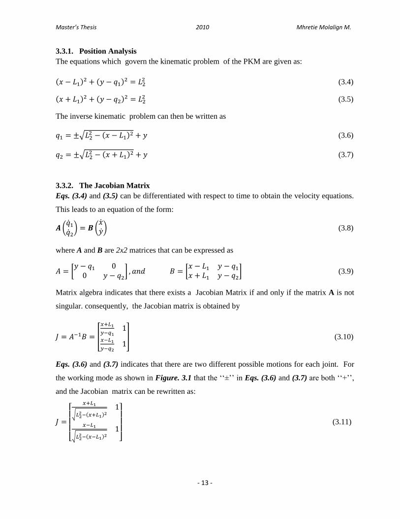
3.3.1. Position Analysis
The equations which govern the kinematic problem of the PKM are given as:
(3.4)
(3.5)
The inverse kinematic problem can then be written as
(3.6)
(3.7)
3.3.2. The Jacobian Matrix
Eqs. (3.4) and (3.5) can be differentiated with respect to time to obtain the velocity equations.
This leads to an equation of the form:
(3.8)
where A and B are 2x2 matrices that can be expressed as
(3.9)
Matrix algebra indicates that there exists a Jacobian Matrix if and only if the matrix A is not
singular. consequently, the Jacobian matrix is obtained by
(3.10)
Eqs. (3.6) and (3.7) indicates that there are two different possible motions for each joint. For
the working mode as shown in Figure. 3.1 that the „„±‟‟ in Eqs. (3.6) and (3.7) are both „„+‟‟,
and the Jacobian matrix can be rewritten as:
(3.11)

Master’s Thesis 2010 Mhretie Molalign M.
- 14 -
3.3.3. Velocity and Acceleration Analysis
Having the position vectors of the end-effector P and the joints Q from Eq. (3.1) and Eq.
(3.2), respectively, and then, with direct kinematic analysis the end effector position P can be
stated as a function of the joint position Q by a set of closed-form equations.
(3.12)
Consequently, the joint space velocities at the slider-leg junctions, point B1 and B2 can be
calculated as follows
(3.13)
Where J is the Jacobian matrix obtained in Eq. (3.11). Similarly the joint space acceleration
can be obtained from the known end-effector motion and the already determined joint position
Q and joint velocity .
(3.14)
where
(3.15)
3.4. Direct Kinematic Problem
3.4.1. Direct analysis for position
The direct kinematic analysis is concerned about obtaining the end-effector motion (Position,
velocity and acceleration) when the joint motion is given or known from the output of
actuators. In this case, for the position of the end-effector the value of x and y can be found as
follows as a function of the joint positions q1 and q2.
(3.16)

Master’s Thesis 2010 Mhretie Molalign M.
- 15 -
(3.17)
3.4.2. Direct analysis for velocity and acceleration
The end-effector velocity and acceleration can be determined from the joints motion. And, the
equations which govern this analysis are given below in Eq. (3.18) and (3.19), respectively.
(3.18)
(3.19)
3.5. Singularity Conditions
Most of the times, kinematic singularity leads to a loss of the controllability and degradation
of the natural stiffness of manipulators, as a result the analysis of parallel manipulators has
drawn considerable attention. In some configurations, the robot cannot be fully controlled.
Most parallel manipulator suffer from the presence of singular configurations in their
workspace that limit the machine performances. In the case of parallel manipulators and
closed-loop mechanisms, singularity analysis is much more difficult since such mechanisms
contain unactuated joints and joints with more than one degree of freedom[ref4]. In general,
closed-form solutions for singular curves/surfaces for parallel manipulators of arbitrary
architecture requires elimination of unwanted variables from several nonlinear transcendental
equations, and this is quite difficult.
Based on the forward and inverse Jacobian matrices, three kinds of singularities of parallel
manipulators can be obtained [24]. Let q denote the actuated joint variables, and let p describe
the location of the moving platform. The kinematic constraints imposed by the arms of the
manipulator are expressed as f(x, q)=0. Differentiating with respect to time, a relation between
the input joint rates and the end effector output velocity is obtained as:
(3.20)
Where,
and
. Which leads to the overall Jacobian matrix J, can be written as:
(3.21)

Master’s Thesis 2010 Mhretie Molalign M.
- 16 -
It is said that singular configurations should be avoided at any cost. The singular
configurations (also called singularities) of a parallel robot may appear inside the workspace
or at its boundaries.
3.5.1. The first kind of singularity
The first kind of singularity occurs when the following condition is satisfied:
This kind of singularity corresponds to the limit of the workspace. Where, the end-effector
point P moves to either extremes sides of the work envelop resulting in constraint violation.
3.5.2. The second kind of singularity
The second kind of singularity occurs when we have following:
,
The physical interpretation of this kind of singularity is that even if all of the input velocities
are zero, there are still be instantaneous motion of the end-effector. In this configuration, the
manipulator loses stiffness and becomes uncontrollable. This kind of singularity is located
inside the workspace of the manipulator. Such a singularity is very difficult to locate only by
analyzing and expanding the equation . A numerical method is thus a good
selection for solving this problem.
3.5.3. The third kind of singularity
The third kind of singularity occurs when both:
This kind of singularity corresponds to the first and second type of singularity occurring
simultaneously. This singularity is both configuration and architecture dependent.
Parallel singularities are particularly undesirable because they cause the following problems:
a high increase of forces in joints and links, that may damage the structure,
a decrease of the mechanism stiffness that can lead to uncontrolled motions of the tool though
actuated joints are locked. [44]

Master’s Thesis 2010 Mhretie Molalign M.
- 17 -
Figure 3.3 Singularity configuration of a PKM 2-DoF manipulator
Figure 3.4 Singularity configuration of a PKM 2-DoF manipulator
Figure 3.5 Singularity configuration of a PKM 2-DoF manipulator

Master’s Thesis 2010 Mhretie Molalign M.
- 18 -
3.6. Solidworks modeling
Before leading to the full inverse kinematic analysis in Matlab/Simulink it is necessary to
create a physical model of the manipulator in Solidworks environment, and then, to translate
that into a Matlab/Simulink-SimMechanics compatible format. All the dimensions of the robot
are assumed to be as follows:
2*L1 = 500 mm is the distance between sliders
L = 1500 mm is the length of both the cylinders (maximum stroke)
L2 = 354 mm is the length of the two arms
d=30 mm is the diameter of the arm rods
dc=32 mm is the bore diameter of the cylinder
The three dimensional (3D) model built in Solidworks in shown below in Figure 3.6. Each of
the components are created separately in Solidworks components design module as shown in
Figure 3.7, and then brought together in the assembly module to create the complete
manipulator. Though it is possible to study the kinematics of the manipulator in Solidworks
environment, it has not tried here because it is more direct and understandable in a
Matlab/Simulink environment.
Figure 3.6 A 3D physical model of the complete PKM manipulator created with Solidworks
Slider
s
Base
Arms
End-effector
Slider
s

Master’s Thesis 2010 Mhretie Molalign M.
- 19 -
Figure 3.7 Solidworks individual component model for the PKM manipulator
a) Base
b) Slider
c) Arm and
d) End-effector
c
a b
c d

Master’s Thesis 2010 Mhretie Molalign M.
- 20 -
3.7. Numerical Simulation for the Inverse Kinematic Analysis
For the Kinematic analysis, a model is developed in Simulink including the physical model of
the manipulator designed in Solidworks (shown in Figure 3.6) and exported to Simulink-
SimMechanics. The necessary steps and assumptions for the development of a physical model
in Solidworks are discussed in the previous chapter under the topic Solidworks modeling,
hence here it is only presented the final entire model of the manipulator. Figure 3.8, below,
shows the complete Matlab/Simulink + Solidworks model developed for the kinematic
analysis of the parallel manipulator
Figure 3.8 A complete model of the PKM manipulator on a Simulink environment
3.7.1. Description of sections in Simulink model
Section 1: This section has contained the input to the program. It is the vector of the desired
trajectory X-axis and Y-axis components against the motion time t. In general these inputs are
functions of all known parameters, such as: the desired trajectory, the desired motion law and
the motion time. More on the choice of motion law will be discussed in chapter 5 .However, at
this stage a circle of radius r=100mm is used as the desired trajectory. Whereas, the law of
motion is assumed to be a symmetric constant acceleration law with a motion time of T=10
seconds.
[X_r , Y_r]
[X,Y]
y_r
x_r
y
xq1
q2
dq1
dq2
ddq1
ddq2
(x,y ,z)
Manipulator
x_r
y _r
q1_r
q2_r
q1d_r
q2d_r
q1dd_r
q2dd_r
Inverse kinematic
xy z
x
y
Filteryy_r
Desired Y-axis trajectory
xx_r
Desired X-axis trajectory
1 2 3 4
5

Master’s Thesis 2010 Mhretie Molalign M.
- 21 -
Section 2: This section is the major step in the Inverse Kinematic Analysis (IKA) of the
manipulator. Through the inverse Kinematic Analysis equations discussed above, the joint
space motion is determined as a function of the end-effector [ P(x, y)] motion. The
mathematical algorism which cover this section in written in the Matlab code file which is
namedas main_kinematic.m. For more detail regarding the implemented Matlab codes the
reader is advised to refer to the functions given in Appendix-A Part I. Similarly, the IKA can
totally be done in Simulink space as shown in Figure 3.9, blow.
Figure 3.9 Inverse Kinematic Analysis (IKA):- Simulink based model
Section 3: In this section, the physical model created in Solidworks and transformed in to
Matlab/Simulink environment is provided with the necessary motion input at the joints. It
introduces functions and at points B1 and B2 , respectively, and
induces a kinematic simulation of the PKM manipulator. Figure 3.10, below, shows the
translated model in a Simulink-SimMechanics environment.
Section 4: This section display the resulting trajectory simulation while the main program is
executed. It is designed to display all the trajectory points in an X-Y plane plot, which in deed
is lied inside the workspace of the PKM manipulator.
6
q2dd_r
5
q1dd_r
4
q2d_r
3
q1d_r
2
q2_r
1
q1_r
x_r ufcn
fcn2
x_r ufcn
fcn1
A
y _r
J
x_r
q1dd_r
q2dd_r
fcn
Qd1
x_r
y _r
J
q1d_r
q2d_r
fcn
Qd q1_r
y d_r
q2_r
q2d_r
q1d_r
x_r
y _r
Afcn
Matrix A
x_r Jfcn
Jacobian Matrix
du/dt
Derivative
2
y_r
1
x_r

Master’s Thesis 2010 Mhretie Molalign M.
- 22 -
Figure 3.10 Model of PKM Manipulator in a SimMechanics interface
The same model with all the input motions applied at joints 1 and 2, is shown in Figure 3.11.
In this model, the mechanical system is given a genaralized motion (position, velocity and
aceeleration) at the joints through a SimMechanics library block joint actuator attached to
prisimatic joints and the response motion is obtained through body sensors block attached to
any of the desired linkages.
Figure 3.11 Model in Simmechanics with desired motion as an input for kinematic analysis
Section 5: This section gives the simulated plot of the desired trajectory given by the user as
an input, by a similar fashion discussed in section 4, above.
3.7.2. Results and discussions
Both the Matlab based and Simulink based analysis results in same output. The desired
trajectory, assumed to be a circle, is shown in Figure 3.12 below,
CS2 CS3
slider2-1
CS2 CS3
slider1-1
CS2 CS3
leg2-1
CS2 CS3
leg1-1
CS2
CS3
end-1
CS2
CS3
CS4
base-1
B F
Weld1
B F
Weld
CS3 CS2
RootPartRootGround
B F
Revolute3
B F
Revolute2
B F
Revolute1
B F
Revolute
B F
Prismatic1
B F
Prismatic
Env
1
(x,y,z)
CS2 CS3
slider2-1
CS2 CS3
slider1-1
CS2 CS3
leg2-1
CS2 CS3
leg1-1
CS2
CS3
CG
end-1CS2
CS3
CS4
base-1
B F
Weld1
B F
Weld
CS3 CS2
RootPartRootGround
B F
Revolute3
B F
Revolute2
B F
Revolute1
B F
Revolute
B
F
Prismatic1
B
F
Prismatic
Env
Joint Actuator2
Joint Actuator1
Body Sensor
6
ddq2
5
ddq1
4
dq2
3
dq1
2
q2
1
q1

Master’s Thesis 2010 Mhretie Molalign M.
- 23 -
Figure 3.12 Desired Trajectory
Whereas, the plot of a symmetric constant acceleration law, which is chosen to be the
governing motion law for the kinematic analysis is given in Figure 3.13.
Figure 3.13 Desired motion law (A symmetric Constant Acceleration Law)
-0.1 -0.05 0 0.05 0.1-0.1
-0.08
-0.06
-0.04
-0.02
0
0.02
0.04
0.06
0.08
0.1Desired Trajectory
0 1 2 3 4 5 6 7 8 9 100
2
4
6
8
t [s]
theta
[ra
d]
End-effector Desired Motion Law
0 1 2 3 4 5 6 7 8 9 100
0.5
1
t [s]
d(t
heta
) [r
ad/s
]
0 1 2 3 4 5 6 7 8 9 10-0.4
-0.2
0
0.2
0.4
t [s]
d2(t
heta
) [r
ad/s
2]
Master’s Thesis 2010 Mhretie Molalign M.
- 24 -
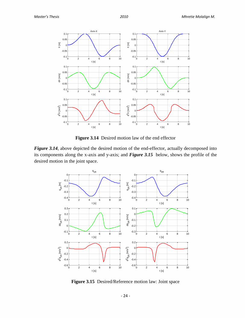
Figure 3.14 Desired motion law of the end effector
Figure 3.14, above depicted the desired motion of the end-effector, actually decomposed into
its components along the x-axis and y-axis; and Figure 3.15 below, shows the profile of the
desired motion in the joint space.
Figure 3.15 Desired/Reference motion law: Joint space
0 2 4 6 8 10-0.1
-0.05
0
0.05
0.1Axis-X
t [s]X
[m
]
0 2 4 6 8 10-0.1
-0.05
0
0.05
0.1
t [s]
dX
[m
/s]
0 2 4 6 8 10-0.1
-0.05
0
0.05
0.1
t [s]
d2X
[m
/s2]
0 2 4 6 8 10-0.1
-0.05
0
0.05
0.1Axis-Y
t [s]
X [
m]
0 2 4 6 8 10-0.1
-0.05
0
0.05
0.1
t [s]
dX
[m
/s]
0 2 4 6 8 10-0.1
-0.05
0
0.05
0.1
t [s]d
2X
[m
/s2]
0 2 4 6 8 10-0.4
-0.3
-0.2
-0.1
0
q1R
t [s]
q1R [
m]
0 2 4 6 8 10-0.1
0
0.1
0.2
0.3
t [s]
dq
1R [
m/s
]
0 2 4 6 8 10-0.6
-0.4
-0.2
0
0.2
t [s]
d2q
1R [
m/s
2]
0 2 4 6 8 10-0.4
-0.3
-0.2
-0.1
0
q2R
t [s]
q2R [
m]
0 2 4 6 8 10-0.3
-0.2
-0.1
0
0.1
t [s]
dq
2R [
m/s
]
0 2 4 6 8 10-0.6
-0.4
-0.2
0
0.2
t [s]
d2q
2R [
m/s
2]

Master’s Thesis 2010 Mhretie Molalign M.
- 25 -
Chapter Four
4. Dynamic modeling and Analysis
The dynamic model of the PRRRP PKM manipulator focuses on analyzing the response motion of the
manipulator for a given action of the driving actuator, in this case a pneumatic one. Therefore, this
chapter deals with, first, on determining the desired action forces need to be applied by the actuators
through an inverse dynamic analysis. Then, it discusses modeling of a pneumatic servo drive in the
Matlab/Simulink environment. Finally, it shows how to create a complete dynamic model, analyze the
model and discuss the resulting response.
4.1. Dynamic Analysis Approaches In robotics literature, there are two basic approaches to dynamics, namely Newton-Euler and
Lagrangian. For the former, one first carry out a detail force and torque analysis of each rigid link with
some physical knowledge such as Newton‟s third law, and then apply Newton‟s law and Euler‟s
equation to each of the rigid links to obtain a set of 2nd order Ordinary Differential Equations (ODE)
in the position and angular representation of each rigid link. Finally together with the kinematic
constraints, the set of equations can be simplified or solved, till the desired form of dynamics equation
is obtained. The Lagrangian approach is a more elegant and tractable one which involve the choice of a
set of generalize coordinates to describe the configuration of the system, and the setting up of a scalar
function called Lagrangian in the tangent bundle of the configuration space.
4.1.1. The Newton-Euler approach In this approach, first it is necessary to isolate all the rigid links of the system. Then, attach a frame at
the center of mass of each rigid link. All the forces and torques applied to each rigid link must be
considered. For the forces or torques which are action and reaction pairs are considered to have the
same magnitude, opposite directions and act on different bodies along the same line of action
according to Newton‟s third law.
The advantage of this approach is that the formulation is globally valid, i.e. independent of the choice
of coordinate system. It is also more intuitive with physical meanings. In literature, there are many
variations for the above method, which is basically the difference of a choice of coordinate systems
(e.g. body or spatial frame) to describe the various quantities in the systems. In Newton-Euler
formulation, in principle, we can account for all the forces and torques applied to each individual link
in the systems and derive the equations of motion.[9]

Master’s Thesis 2010 Mhretie Molalign M.
- 26 -
4.1.2. Lagrangian approach
The Lagrangian formulation describes the behavior of a dynamic system in terms of work and energy
stored in the system rather than in terms of force and moments of the individual members involved.
Using this approach, the closed-form dynamical equations can be derived systematically in any
coordinate system. In this paper, Lagrange‟s equation using constrained coordinates (i.e. the Lagrange
multiplier approach) is presented:
(4.1)
where i is the constraint index, j is the generalized coordinate index, k is the number of
constraint functions, K is the total kinetic energy of system, U is the total potential energy
term, ςi is the Lagrange multiplier, Gij is the element of the Jacobian matrix of constraint
equation, Gij = ∂fi/∂qj, where fi is a constraint equation, qj the jth
generalized coordinate.
4.2. Inverse Dynamics Analysis through the Newton-Euler approach The vectors closed-loop of one leg is shown in Figure 4.1. A fixed leg frame B–x‟y‟ is
established at the point B and parallel to the global frame O-x y. A local leg frame is also
established at the point B while its x-axis is along the leg length direction and its z-axis is
parallel to that of the global frame. The vector which represents the inverse kinematic
equation of aforementioned closed-loop can be given as
r= b + qe2 + Lw (4.2)
Figure 4.1. Position analysis for a single leg of the PKM manipulator
r
x
B
x
P
Lwi
x’
y
y’ y
bi
qie2
y’
x’
Q O

Master’s Thesis 2010 Mhretie Molalign M.
- 27 -
where r = [x y]T is the position vector of P with respect to the global frame O-xy, b=[xB 0]
T is
the position vector of Q with respect to the global frame, and e2=[0 1]T. q is the y coordinate
of point B and L and w are the length and unit vector of the leg, respectively, with respect to
the global frame. As it is discussed in detail in chapter three, there are four inverse kinematic
solutions for a given position of platform. In the configuration shown in Figure 3.1,
(4.3)
(4.4)
Where in Eq. 4.4, for the configuration shown in Figure 3.1, ‘ + ’ for leg number one and
‘ - ‘ for leg number two. Then, the joint position vector q for a single leg can be obtained as:
(4.4)
Form the time derivative of Eq. 4.2, the velocity of the joint is obtained as:
(4.6)
Multiplying both sides of Eq. 4.6 by wT results in ,
(4.7)
(4.8)
Taking the dot product of with both sides of Eq. 4.6 yields in the angular velocity
of the leg.
(4.9)
Further, the time derivative of Eq. 4.6 gives the following equation which, in turn can be
rearranged to give a vector of accelerations of the joint, as shown:
(4.10)
Master’s Thesis 2010 Mhretie Molalign M.
- 28 -
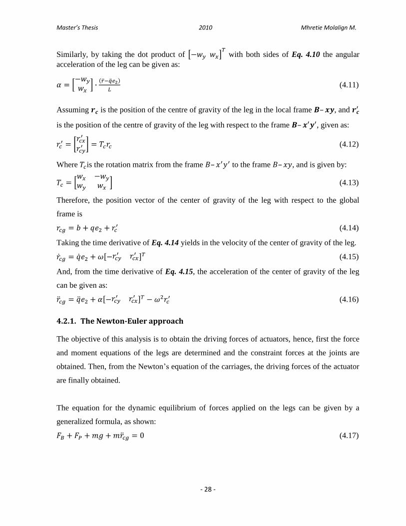
Similarly, by taking the dot product of with both sides of Eq. 4.10 the angular
acceleration of the leg can be given as:
(4.11)
Assuming is the position of the centre of gravity of the leg in the local frame – , and
is the position of the centre of gravity of the leg with respect to the frame – , given as:
(4.12)
Where is the rotation matrix from the frame – to the frame – , and is given by:
(4.13)
Therefore, the position vector of the center of gravity of the leg with respect to the global
frame is
(4.14)
Taking the time derivative of Eq. 4.14 yields in the velocity of the center of gravity of the leg.
(4.15)
And, from the time derivative of Eq. 4.15, the acceleration of the center of gravity of the leg
can be given as:
(4.16)
4.2.1. The Newton-Euler approach
The objective of this analysis is to obtain the driving forces of actuators, hence, first the force
and moment equations of the legs are determined and the constraint forces at the joints are
obtained. Then, from the Newton‟s equation of the carriages, the driving forces of the actuator
are finally obtained.
The equation for the dynamic equilibrium of forces applied on the legs can be given by a
generalized formula, as shown:
(4.17)

Master’s Thesis 2010 Mhretie Molalign M.
- 29 -
Where m is the mass of the leg g is the gravitation acceleration, assuming a horizontal or X-Y
work table, g=[0 0]T. FP=[FPx FPy]
T and FB=[FBx FBy]
T are the forces exerted on the leg by
the end effector and actuator/slider, respectively.
Applying Newton‟s equation for end effector, yields in:
(4.18)
Where M is the mass of the end-effector, and Fext =[Fx Fy]T is the external force exerted on
the end-effector.
Besides, the moment equations of a single leg about point B are given as :
(4.19)
where
is the moment of inertia of the leg to point B. Moment equation of the end-
effector about point P.
(4.20)
Where is the external moment applied on the end-effector and Rc=[Rcx Rcy]T is the
position vector of the center of the end-effector with respect to the frame P-x’y’. i.e. Rc=[0
0]T. Finally, Eqs. 4.18, 4.19 and 4.20 are combined into a single linear system of equation in the form
shown below.
(4.21)
Where,
and
Then, the solution of Eq. 4.21 yields in the desired forces at point P.

Master’s Thesis 2010 Mhretie Molalign M.
- 30 -
(4.22)
The forces exerted on the legs by the sliders at the point B, FB=[FB1 FB2]T can be obtained as:
(4.23)
From Newton equation applied on the sliders, the driving forces of the actuators can be
derived.
The Newton equation for the left actuator:
(2.24)
Similarly, the Newton‟s equation for the right side actuator:
(2.25)
Where Fd1 and Fd2 are the desired drive forces, N1 and N2 are reaction forces along the x-axis,
ms and ma are mass of the slider and actuator, respectively. fbw is the friction force due to
actuator-slider interaction. Hence, the drive forces can be extracted from Eqs. 2.24 and 4.25:
(4.26)
With the desired drive forces known, the dynamic analysis of the manipulator leads to the next
step of modeling a pneumatic actuator which can provide force. Hence, the purpose of the
next section would be on modeling a pneumatic drive system that consists of a valve (most
probably a proportional directional control valve), a cylinder-piston system and pipe lines and
the various connection between them.

Master’s Thesis 2010 Mhretie Molalign M.
- 31 -
4.3. Pneumatic Servo System Modeling
4.3.1. Pneumatic Actuators: Modeling
Several approaches have been proposed for modeling the pneumatic actuators. One of the
widely used methods for finding the mathematical model of the pneumatic actuator is a
theoretical analysis. The analysis of pneumatic actuators requires a combination of
thermodynamics, fluid dynamics and the dynamics of the motion. For constructing a
mathematical model, three major considerations must be involved:
1. The determination of the mass flow rates through the valve.
2. The determination of the pressure, volume and temperature of the air in cylinder.
3. The determination of the dynamics of the load.
Accurate model of pneumatic actuator is an important condition both for control design and
for optimizing its operation. As a result, this chapter is concerned with the mathematical
modeling and numerical simulation for pneumatic actuator systems. [30]
4.3.2. Pneumatic Actuators: The Control Strategies:
The advantages of pneumatic systems are well known as clear, cheap, easily maintained, safe
in operation, etc. But for their highly nonlinear properties such as compressibility of medium,
friction effect and nonlinearity of valves, pneumatic actuators are seldom used in industrial
servo applications. Moreover, some of their properties, e.g., poor damping, low stiffness, and
limited bandwidth, are unfavorable in the servo control system design.
Some other difficulties in the control of pneumatic servo systems are the possible presence of
unknown disturbances coming from leakage of valves, time-varying payloads, and external
perturbations. Besides, uncertainties in system parameters make the controller design problem
more challenging [30]. To cope with some of these problems, advanced control algorithms
have to be proposed.
4.3.3. The Dynamic Model
The dynamic model used in this work is developed based on:
1. the description of the relationship between the air mass flow rate and pressure changes
in the cylinder chambers, and
2. the equilibrium of the forces acting at the piston, including the friction force.

Master’s Thesis 2010 Mhretie Molalign M.
- 32 -
A schematic view of the system to be modeled is shown in Figure 4.2.The relationship
between the air mass flow rate and the pressure changes in the chambers is obtained using
energy conservation laws, and the force equilibrium is given by Newton‟s second law. The
friction force and the external forces are modeled in a unified way.
Figure 4.2 Schematic of a Pneumatic Drive System. Source ref. [30]
4.3.3.1. Conservation of Energy
The internal energy of the mass flowing into chamber 1 is Cpqm1T , where Cp is the constant
pressure specific heat of the air, T is the air supply temperature, and
is the air
mass flow rate into chamber 1. The rate at which work is done by the moving piston is p1 1 ,
where p1 is the absolute pressure in chamber 1 and
is the volumetric flow rate.
The time air internal energy change rate in the cylinder is
, where CV is the constant
volume specific heat of the air and ρ1 is the air density. We consider the ratio between the
specific heat values as r = CP /CV and that ρ1=CV/( RT) for an ideal gas, where R is the
universal gas constant. An energy balance yields:
(4.27)

Master’s Thesis 2010 Mhretie Molalign M.
- 33 -
The total volume of chamber 1 is given by V1 = Ay +V10 , where A is the cylinder cross-
sectional area, y is the piston position and V10 is the dead volume of air in the line and at the
chamber 1 extremity. The change rate for this volume is , where
is the
piston velocity. After calculating the derivative term in the right hand side of Eq. 4.27, and
assuming air is a perfect gas undergoing an isothermal process, the rate of change of the
pressure inside each chamber of the cylinder can be expressed as:
(4.28)
(4.29)
where Cp = (kR) /(k −1) and L is the maximum cylinder stroke. Assuming that the mass flow
rates are nonlinear functions of the servovalve control voltage (u) and of the cylinder
pressures, that is, qm1 = qm1( p1,u) and qm2 = qm2 ( p2 ,u) , Eq. 2.28 and Eq. 2.29 result in,
(4.30)
(4.31)
Therefore, incorporation all the above nonlinear sets of equations, the resulting scheme of the
pneumatic drive looks like Figure 4.3, below.
Figure 4.3 Pneumatic drive and mechanical subsystem scheme
Where u is the command signal from the controller/regulator. The Matlab/Simulink model
created based on the kinematic and dynamic equations of the PKM manipulator and equations
that govern the nonlinear behavior of the pneumatic drive is shown below, in Fig. 4.4.
Pneumatic
Subsystem
Mechanical
Subsystem
u y

Master’s Thesis 2010 Mhretie Molalign M.
- 34 -
Figure 4.4 Complete dynamic model of the PKM manipulator built in Matlab/Simulink
The detail Matlab code for the dynamic analysis can be found in Appendix-A part I by the name of
main_dynamic.m and I_dynamic.m. Also, the detail of the various subsystem blocks in Figure 4.4 are
presented in Appendix-A part II.
q2
q1
u1
u2
F1
F2
q2d
q1d
x
y
xy zy
xy zy
xy zy
xy zy
manipulator
cylinder2
cylinder1
PID
controller
XY Graph
q2_r
q1_r
In1
Out1
Out2
Filter

Master’s Thesis 2010 Mhretie Molalign M.
- 35 -
4.4. Simulation results and Discussion
4.4.1. Thermal and physical characteristics of the pneumatic drive
In order to carryout a dynamic numerical simulation the following considerations has been
taken.
Table 4.1 Value of Physical and Thermal Constants
Parameter Description Ps=6*10
5 Pa Cylinder supply pressure
Pe=1*105 Pa Cylinder exhaust pressure
Pa=101.3*103 Pa Atmospheric pressure
P0=3*105 Pa Initial pressure inside cylinder chambers
Cr=0.852 Critical pressure ratio
Ts=Tc=Te=293 K Ts-Supply air temperature, Tc-cylinder chamber temperature, and Te-
exhaust air temperature. Assuming an isothermal process.
C1=3.864 Valve constant
C2=0.04 Valve constant
Cp The constant pressure specific heat of the air
CV The constant volume specific heat of the air
k=1.4 Heat ratio
R=287 m.K-1
Gas constant
B=65 Nsm-1
Viscous friction coefficient of air
Cd=0.8 Valve discharge coefficient
Table 4.2 Pneumatic cylinder characteristics
Model FESTO DGP/DGPL
Size (Bore) 32 [mm]
Maximum stroke (Length) 3000* [mm]
Base weight 1550 [g]
Operating Medium Filtered compressed air, unlubricated or lubricated [min. 40 μ]
Operating Pressure 2 - 8 [bar]
Ambient Temperature 10 to 60 [°C]
Table 4.3 Proportional valve characteristics
Model MPYE Proportional directional control valve
Valve Function 5/3-way, normally closed
Construction design Piston spool, directly actuated, controlled spool position
Sealing principle hard
Actuation type Electrical
Type of rest Mechanical spring
Type of pilot control Direct
Direction of flow Non-reversible
Type of mounting Via through-holes
Mounting position any

Master’s Thesis 2010 Mhretie Molalign M.
- 36 -
4.4.2. Simulink model of pneumatic system
A detailed model of the pneumatic drive system is created, in a Simulink environmet, based on
the equations from Eq. 4.27 to Eq. 4.31 and using the data given in Tables 4.1, 4.2 and 4.3.
The resulting design is shown in Figure 4.5, below.
Figure 4.5 Detailed Simulink model of a pneumatic actuator
This subsystems receives a command u, position and speed feedback q and , and it gives the
change in pressure between chamber A and B. Which then multiplied by the cross-sectional
area of the piston Ap and results in the desired force F need to be applied at the manipulators
joint.
1
F1
Ps0:0
ps
Pa
Ps
Xa
Pe
Pb
dma
dmb
flow rate
dmb
Pb
dx
x
dPb
chamberB
x
dx
Pa
dma
dPa
chamberA
Pe0:0
Pe1
s
Integrator1
1
s
Integrator
-K-
Ap
3
u1
2
q1
1
dq1

Master’s Thesis 2010 Mhretie Molalign M.
- 37 -
Chapter Five
5. Control Strategies
The advantages of pneumatic systems are well known such as clear, cheap, easily maintained,
safe in operation, etc. But for their highly nonlinear properties such as compressibility of
medium, friction effect and nonlinearity of valves, pneumatic actuators are seldom used in
industrial servo applications. Moreover, some of their properties, e.g., poor damping, low
stiffness, and limited bandwidth, are unfavorable in the servo control system design. Some
other difficulties in the control of pneumatic servo systems are the possible presence of
unknown disturbances coming from leakage of valves, time-varying payloads, and external
perturbations. Besides, uncertainties in system parameters make the controller design problem
more challenging.
5.1. A Review of Control strategies The problem of controlling robots has been extensively important in most of industrial
applications. A great variety of control approaches have been proposed throughout the years.
The most common which is in use with present industrial robots is a decentralized
"proportional, integral, derivative" (PID) control for each degree of freedom. More
sophisticated nonlinear control schemes have been developed, such as so-called computed
torque control, termed inverse dynamic control, which linearizes and decouples the equation
of motion of the robot. In this chapter, first it is discussed the pros and cons PID with respect
to other control schemes, i.e. a classical PID control, Sliding mode control, and then the
nonlinear linearizing and decoupling control schemes. Then, it focuses on PID controller
modeling and tuning based on the need to obtain a good trajectory tracking.
In case of pneumatic drive PID controller is still the most widely used approach due to its ease
of implementation, the need for overcoming highly nonlinear phenomena turns away the use
of classical PID controllers nowadays, see [4]. Therefore modern control techniques were
designed and tested in pneumatic actuators in order to improve the performance of such
systems considering position accuracy and repeatability as the two main performance
characteristics. Fuzzy logic control, neural networks method, adaptive control, self-tuning or

Master’s Thesis 2010 Mhretie Molalign M.
- 38 -
gain scheduling, the so-called “Soft Computing” control techniques, are approaches that have
attracted many researchers.
5.1.1. PID Controller
The dynamic model is described by a system of n coupled nonlinear second order differential
equations, n being the number of joints. However, for most of today's industrial robots, a local
decentralized "proportional, integral, derivative" (PID) control with constant gains is
implemented for each joint. The advantages of such a technique are the simplicity of
implementation and the low computational cost. The drawbacks are that the dynamic
performance of the robot varies according to its configuration, and poor dynamic accuracy
when tracking a high velocity trajectory. In many applications, these drawbacks are not of
much significance.
The control law is given by:
(5.1)
Where is the position error at the joint. The objective function is, then, to get a
quality trajectory tracking by minimizing the error in joint position through a compensation of
the nonlinearities in the pneumatic drive system.
Practically, the block diagrams of such a control scheme is shown in Figure 5.1.
Figure 5.1 PID controller block diagram
5.2. PID Controller Design and tuning The design is done using a Simulink PID Controller Block , from library:
Simulink/Continuous in Matlab. This block takes an error signal and tends to give a tuned
value of the gain constants. The PID block is shown in Figure 5.2.

Master’s Thesis 2010 Mhretie Molalign M.
- 39 -
Figure 5.2 PID controller Block in Simulink library
5.2.1. Position Control
As it can be seen from Figure 4.4, the control for trajectory tracking is performed on the joint
position. Indirectly, the position of the actuated joints which is also known as the cylinder
piston displacement is compared with the desired joint position.
To be Continued …
2
u2
1
u1
PID(s)
PID Controller1
PID(s)
PID Controller
4
q2
3
q2_r
2
q1_r
1
q1

Master’s Thesis 2010 Mhretie Molalign M.
- 40 -
Conclusions
The objective of this thesis work was to carry out a full kinematic and dynamic analysis of a 2
DoF planar PKM manipulator driven by a pneumatic actuator. Thereby, to devise an
appropriate control strategy in order to eliminate the position error that might be induced due
to the nonlinearity in the drive mechanism.
Accordingly, in third chapter, it is presented detailed kinematic analysis. The model used in
the kinematic simulation is designed in a Matlab/Simulink environment and it includes a
physical representation of the manipulator created in Solidworks interface and then translated
into a Simmechanics equivalent. The response of the manipulator for a desired input
trajectory, in this case a circle under the effective work-envelop and desired motion law, i.e. a
symmetric constant acceleration law, was as expected. Means, there isn‟t position error due to
only the kinematic of the mechanism because, it has been assumed that all the linkages in the
PKM manipulator are rigid.
Whereas, as it is presented in the subsequent chapters, four and five, it has been tried to make
a full dynamic analysis, which includes modeling of a pneumatic drive in a Matlab/Simulink
environment. A model of the pneumatic actuator is created, as it is stated in chapter four,
based on a set of nonlinear state flow and thermal equations. However, at the end of the
analysis it appears to have a problem on the control of the resulting response. i.e. the
manipulator very hardly follows the desired circular trajectory. As a result, I have faced
difficulties on designing a control scheme that can compensate this huge gap in position.
Having spent too much effort and time on finding/creating a pneumatic actuator model that
may result in a reasonable response, I still couldn‟t overcome this difficulty. Therefore, due to
lack of additional time, my limited scope of knowledge on pneumatics and also the economic
situation I am in now, I am forced to compile the unfinished work that I have done so far.
Which I hope leads me to my graduation.

Master’s Thesis 2010 Mhretie Molalign M.
- 41 -
Appendix A
1. Part I - Program Details
Detail of the Matlab Code Written for Inverse Kinematic Analysis
main_kinematic.m %%%%%%%%%%%%%%%%%%%%%%%%%%%%%%%%%%%%%%%%%%%%%%%%%%%%%%%%%%%%%%%%%%%%%%%%%%% %Master’s Thesis %Title: Dynamic Analysis of a Planar Manipulator Driven by Pneumatic %Actuators
%By:Mhreite Moalign Mulusew %Supervisors: Eng Hermes Giberti and Ing Simone Cinquemanii %%%%%%%%%%%%%%%%%%%%%%%%%%%%%%%%%%%%%%%%%%%%%%%%%%%%%%%%%%%%%%%%%%%%%%%%%%% %NOTE: This Matlab program is written for the kinematic analysis of the %manipulator. To be fully functional, this program requires the following %Matalb and Simulink files: 1) Constant_Acceleration_ND.m % 2) sim_kinematics.mdl %All the above files should be placed in same folder(directory) that %contains this main program. %%%%%%%%%%%%%%%%%%%%%%%%%%%%%%%%%%%%%%%%%%%%%%%%%%%%%%%%%%%%%%%%%%%%%%%%%%% clear all close all clc
%Robot geometric parameters l1=0.500; %Horizontal distance between the two sliders/actuators [m] l2=0.354; %Length of a single arm [m] l3=1.500; %Maximum length of actuator [m] R1=l1/2; R2=l2;
T=10; %Simulation time[s] t=0:0.1:T; %%------------------------------------------------------------------------- %% %Desired trajectory %Circle Rc=0.1; %Radius of the circle[m] angle=2*pi; %Total angle covered by a circle angle[rad] angle_0=0; %Angle corresponding to initial position [rad] %%------------------------------------------------------------------------- %% %Initial conditions of the manipulator xc=0; %x_position of the center of the circle [m] yc=-0.0790919; %y_position of the center of the circle [m] Dangle=angle-angle_0; Xo=xc+Rc; %Initial x-position of the end effector [m] Yo=yc; %Initial y-position of the end effector [m] vXo=0; %Initial velocity of the manipulator in x-
axis[m/s] vYo=0; %Initial velocity of the manipulator in y-
axis[m/s] %%------------------------------------------------------------------------- %%

Master’s Thesis 2010 Mhretie Molalign M.
- 42 -
% Motion law of the End-Effector (Constant Acceleratin Law) ndt=t./T; par=[1/3,1/3];
[D,V,A] = Constant_Acceleration_ND(ndt,par);
theta=Dangle*D; thetaD=Dangle/T*V; thetaDD=Dangle/T^2*A;
xx=Rc*sin(theta); yy=Rc*(cos(theta)); xd=Rc*thetaD.*cos(theta); yd=Rc*thetaD.*sin(theta); xdd=Rc*(thetaDD.*cos(theta)-(thetaD.^2).*sin(theta)); ydd=Rc*(thetaDD.*sin(theta)+(thetaD.^2).*cos(theta)); %%------------------------------------------------------------------------ %% %%PLOT OF THE DESIRED TRAJECTORY figure('Number','Off','Name','DESIRED TRAJECTORY') plot(xx,yy);grid on;axis equal %%------------------------------------------------------------------------- %% %%END EFFECTOR DESIRED MOTION LAW figure('Number','Off','Name','END-EFFECTOR DESIRED MOTION LAW [SYMMETRIC
CONSTANT ACCELERATION LAW') subplot(311); plot(t,theta,'LineWidth',2);grid on;xlabel('t [s]');ylabel('theta [rad]') subplot(312) plot(t,thetaD,'g','LineWidth',2); grid on;xlabel('t [s]');ylabel('d(theta)
[rad/s]') subplot(313) plot(t,thetaDD,'r','LineWidth',2); grid on;xlabel('t
[s]');ylabel('d^2(theta) [rad/s^2]') %%------------------------------------------------------------------------ %% %%END EFFECTOR DESIRED MOTION LAW DECOMPOSED FOR THE X-AXIS AND Y-AXIS figure('Number','Off','Name','END-EFFECTOR DESIRED MOTION LAW [DECOMPOSED
TO X & Y AXES]') subplot(321); plot(t,xx,'LineWidth',2); title('Axis-X');grid on;xlabel('t
[s]');ylabel('X [m]') subplot(323) plot(t,xd,'g','LineWidth',2); grid on;xlabel('t [s]');ylabel('dX [m/s]') subplot(325) plot(t,xdd,'r','LineWidth',2); grid on;xlabel('t [s]');ylabel('d^2X
[m/s^2]')
subplot(322); plot(t,yy,'LineWidth',2); title('Axis-Y');grid on; xlabel('t
[s]');ylabel('X [m]') subplot(324) plot(t,yd,'g','LineWidth',2); grid on;xlabel('t [s]');ylabel('dX [m/s]') subplot(326) plot(t,ydd,'r','LineWidth',2); grid on;xlabel('t [s]');ylabel('d^2X
[m/s^2]') %%------------------------------------------------------------------------

Master’s Thesis 2010 Mhretie Molalign M.
- 43 -
%% %INVERSE KINEMATIC ANALYSIS
%joint space position q1=yy - sqrt(R2^2 -(xx + R1).^2); q2=yy - sqrt(R2^2 -(xx - R1).^2); Q=[q1;q2];
for i=1:length(t) %Jacobiam matrix J=[(xx(i)-R1)/sqrt(R2^2-(xx(i)-R1).^2) 1; (xx(i)+R1)/sqrt(R2^2-(xx(i)+R1).^2) 1];
%Joint space velocity Qd(:,i)=J*[xd(i);yd(i)]; q1d=Qd(1,:); q2d=Qd(2,:);
%Matrix A(p,pd) A_A=[(xx(i)^2 + yy(i)^2 - 2*yd(i)*Qd(1) + Qd(1).^2)/(yy(i) - q1(i)); (xx(i)^2 + yy(i)^2 - 2*yd(i)*Qd(2) + Qd(2).^2)/(yy(i) - q2(i))];
%Joint space acceleration Qdd(:,i)=J*[xdd(i);ydd(i)] + A_A;
end q1dd=Qdd(1,:); q2dd=Qdd(2,:);
%%------------------------------------------------------------------------- %% %%DESIRED MOTION LOW IN THE JOINT SPACE. MATLAB BASED ANALYSIS figure('Number','Off','Name','REFERENCE MOTION LAW [ JOINT SPACE ]_MATLAB') subplot(321); plot(t,q1); title('q_1_R');grid on;xlabel('t [s]');ylabel('q_1_R [m]') subplot(323) plot(t,Qd(1,:),'g'); grid on;xlabel('t [s]');ylabel('dq_1_R [m/s]') subplot(325) plot(t,Qdd(1,:),'r'); grid on;xlabel('t [s]');ylabel('d^2q_1_R [m/s^2]')
subplot(322); plot(t,q2); title('q_2_R');grid on; xlabel('t [s]');ylabel('q_2_R [m]') subplot(324) plot(t,Qd(2,:),'g'); grid on;xlabel('t [s]');ylabel('dq_2_R [m/s]') subplot(326) plot(t,Qdd(2,:),'r'); grid on;xlabel('t [s]');ylabel('d^2q_2_R [m/s^2]') %%------------------------------------------------------------------------ %% %%VARIABLES THAT CAN BE USED IN SIMULINK AS AN INPUT xx_r=[t;xx]'; yy_r=[t;yy]'; q1_r=[t;q1]'; q2_r=[t;q2]'; q1d_r=[t;Qd(1,:)]'; q2d_r=[t;Qd(2,:)]'; q1dd_r=[t;Qdd(1,:)]';

Master’s Thesis 2010 Mhretie Molalign M.
- 44 -
q2dd_r=[t;Qdd(2,:)]'; %%------------------------------------------------------------------------ %% %%SIMULINK BASED KINEMATIC ANALYSIS open('sim_kinematic.mdl') sim('sim_kinematic') xp=x.signals.values; yp=y.signals.values; xr=x_r.signals.values; yr=y_r.signals.values; tt=x.time; q1_=q1_r1.signals.values; q2_=q2_r1.signals.values; q1d=q1dot_r.signals.values; q2d=q2dot_r.signals.values; q1dd=q12dot_r.signals.values; q2dd=q22dot_r.signals.values; %%------------------------------------------------------------------------- %% %%DESIRED MOTION LAW IN THE JOINT SPACE. SIMULINK BASED ANALYSIS figure('Number','Off','Name','REFERENCE MOTION LAW [ JOINT SPACE
]_SIMULINK') subplot(321); plot(tt,q1_,'LineWidth',2); title('q_1_R');grid on;xlabel('t
[s]');ylabel('q_1_R [m]') subplot(323) plot(tt,q1d,'g','LineWidth',2); grid on;xlabel('t [s]');ylabel('dq_1_R
[m/s]') subplot(325) plot(tt,q1dd,'r','LineWidth',2); grid on;xlabel('t [s]');ylabel('d^2q_1_R
[m/s^2]')
subplot(322); plot(tt,q2_,'LineWidth',2); title('q_2_R');grid on; xlabel('t
[s]');ylabel('q_2_R [m]') subplot(324) plot(tt,q2d,'g','LineWidth',2); grid on;xlabel('t [s]');ylabel('dq_2_R
[m/s]') subplot(326) plot(tt,q2dd,'r','LineWidth',2); grid on;xlabel('t [s]');ylabel('d^2q_2_R
[m/s^2]') %%------------------------------------------------------------------------ %% %%TRAJECTORY COMPARISON AND POSITION ERROR ANALYSIS figure('Number','Off','Name','TRAJECTORY COMPARISON...KINEMATIC ANALYSIS') hold on plot(xr,yr);grid on plot(xp,yp,'r');grid on axis equal
ex=xr-xp; ey=yr-yp;
figure('Number','Off','Name','End-effector Position Error in the X-axis &
Y-axis') subplot(2,1,1); plot(tt,ex),ylim([-2 2]);title('Error along x-axis');grid on;

Master’s Thesis 2010 Mhretie Molalign M.
- 45 -
subplot(2,1,2); plot(tt,ey,'r'),ylim([-2 2]);title('Error along y-axis');grid on;
%%--------------------------E--N--D----------------------------------------
Detail of the Matlab Code Written for a Symmetric Constant Acceleration Law
Constant_Acceleration_ND.m %%%%%%%%%%%%%%%%%%%%%%%%%%%%%%%%%%%%%%%%%%%%%%%%%%%%%%%%%%%%%%%%%%%%%%%%%%% %Master’s Thesis %Title: Dynamic Analysis of a Planar Manipulator Driven by Pneumatic %Actuators %By:Mhretie Moalign Mulusew %Supervisors: Eng Hermes Giberti and Ing Simone Cinquemanii %%%%%%%%%%%%%%%%%%%%%%%%%%%%%%%%%%%%%%%%%%%%%%%%%%%%%%%%%%%%%%%%%%%%%%%%%%% %NOTE: This Matlab Function is written for generating a Symmetric Constant %Acceleration Law. %%%%%%%%%%%%%%%%%%%%%%%%%%%%%%%%%%%%%%%%%%%%%%%%%%%%%%%%%%%%%%%%%%%%%%%%%%%
function [D,V,A] = Constant_Acceleration_ND(x,par)
% Non-dimensional General Constant Acceleration Motion Law % % x = t/tm non-dimensional time % D = non-dimensional displacement % V = non-dimensional velocity % A = non-dimensional acceleration % par(1) = xa+ % par(2) = xa- %par=[1/3,1/3];
xap = par(1); %Positive acceleration part xam = par(2); %Negative acceleration part
cap = 1/(xap*(1-(xap+xam)/2)); cam = 1/(xam*(1-(xap+xam)/2));
for i=1:length(x)
if x(i)>=0 && x(i)<=xap A(i)=cap; V(i)=cap*x(i); D(i)=0.5*cap*x(i)^2; end if x(i)>xap && x(i)<(1-xam) A(i)=0; V(i)=cap*xap; D(i)=cap*xap*(x(i)-xap/2); end if x(i)>=(1-xam) && x(i)<=1 A(i)=-cam; V(i)=cap*xap-cam*(x(i)-1+xam); D(i)=cap*xap*(x(i)-xap/2)-cam/2*(x(i)-1+xam)^2; end end %%--------------------------E--N--D----------------------------------------

Master’s Thesis 2010 Mhretie Molalign M.
- 46 -
Detail of the Matlab Code Written for Direct Kinematic Analysis
D_kinematic.m %%%%%%%%%%%%%%%%%%%%%%%%%%%%%%%%%%%%%%%%%%%%%%%%%%%%%%%%%%%%%%%%%%%%%%%%%%%
%
%Master’s Thesis %Title: Dynamic Analysis of a Planar Manipulator Driven by Pneumatic %Actuators %By:Mhretie Moalign Mulusew %Supervisors: Eng Hermes Giberti and Ing Simone Cinquemanii
%%%%%%%%%%%%%%%%%%%%%%%%%%%%%%%%%%%%%%%%%%%%%%%%%%%%%%%%%%%%%%%%%%%%%%%%%%% %NOTE: This Matlab Function is written for a Direct Kinematics %%%%%%%%%%%%%%%%%%%%%%%%%%%%%%%%%%%%%%%%%%%%%%%%%%%%%%%%%%%%%%%%%%%%%%%%%%%
function [PP]=D_kinematic(Q1,Q2)
global R1 R2 t
for i=1:(length(t)) q1=Q1(i); q2=Q2(i);
a=(q2 - q1)/(2*R1); b=(q1^2 - q2^2)/(4*R1); e=a^2 + 1; g=(b-R1)^2 + q1^2 - R2^2; f=2*a*(b - R1) - q1*2;
y(i)=-(f - sqrt(f^2 - 4*e*g))/(2*e); x(i)=a*y(i)+b; end
PP=[x;y]; %%------------------------------E--N--D------------------------------------
Detail of the Matlab Code Written for Workspace Generation
Workspace.m %%%%%%%%%%%%%%%%%%%%%%%%%%%%%%%%%%%%%%%%%%%%%%%%%%%%%%%%%%%%%%%%%%%%%%%%%%% %NOTE: This Matlab Function is written for generating Workspace Envelop %%%%%%%%%%%%%%%%%%%%%%%%%%%%%%%%%%%%%%%%%%%%%%%%%%%%%%%%%%%%%%%%%%%%%%%%%%%
close all clear all clc
%Input parameters l1=0.500; %mm l2=0.354; %mm l3=1.500;%mm R1=l1/2;

Master’s Thesis 2010 Mhretie Molalign M.
- 47 -
R2=l2;
%%workspace q=0:0.1:1.25; for i=1:length(q) q1=q(i); for j=1:length(q) q2=q(j); Q=[q1;q2]; [x,y]=D_kinematic(Q); plot(x,y,'*') hold on title('Workspace') axis([-0.25,0.25,0,1.5]) end end %%--------------------------E--N--D----------------------------------------
Detail of the Matlab Code Written for Dynamic Analysis
main_dynamic.m
%%%%%%%%%%%%%%%%%%%%%%%%%%%%%%%%%%%%%%%%%%%%%%%%%%%%%%%%%%%%%%%%%%%%%%%%%%% %Master’s Thesis %Title: Dynamic Analysis of a Planar Manipulator Driven by Pneumatic %Actuators
%By:Mhretie Moalign Mulusew %Supervisors: Eng Hermes Giberti and Ing Simone Cinquemanii %%%%%%%%%%%%%%%%%%%%%%%%%%%%%%%%%%%%%%%%%%%%%%%%%%%%%%%%%%%%%%%%%%%%%%%%%% %NOTE: This Matlab program is written for the dynamic analysis of the %manipulator. To be fully functional, this program requires the following %Matalb and Simulink files: 1) Constant_Acceleration_ND.m % 2) Inverse_Dynamics.m , and % 3) sim_dynamics.mdl %All the above files should be placed in same folder(directory) that %contains this main program. %%%%%%%%%%%%%%%%%%%%%%%%%%%%%%%%%%%%%%%%%%%%%%%%%%%%%%%%%%%%%%%%%%%%%%%%%%% clear all close all clc
global l1 l2 R1 J1 J2 M m1 m2 ms mcy g
%Robot geometric parameters l1=0.500; %Horizontal distance bteween the two sliders/actuators [m] l2=0.354; %Length of a single arm [m] l3=1.500; %Maximum length of actuator [m]
%Physical and Thermal Constants Ps=6e5; %Cylinder Supply pressure [Pa] Pe=1e5; %Cylinder Exhaust pressure [Pa] P0=3e5; %Initial pressure in the cylinder [Pa] Patm=101.3e3; %average atmospheric pressure [Pa] Cr=0.852; %Critical pressure ratio[] Ts=293; %Supply temperature [K]

Master’s Thesis 2010 Mhretie Molalign M.
- 48 -
Tc=Ts; %Cylinder temperature [K]...Isothermal process Tp=Ts; %Pipe temperature [K]...Isothermal process Ck=3.864; %Valve constant1[] Co=0.04; %Valve constant2[] Cd=0.8; %valve coeffiecent of discharger[] Cs=Cd; Cc=0.7; %Connection port discharge coefficient [] Cv=3.15745e-4; %Valve constant[m/V] B=65; %Viscous friction coefficient of air[Ns/m] k=1.4; %Heat ratio gam=k; R=287; %Gas constant [m/K] g=0; %Gravitational Acceleration [m/s^2] ms=1; %Mass of slider [kg] mcy=1; %Mass of Cylinder piston [kg] m1=2; %Mass of leg one [kg] m2=2; %Mass of leg two [kg] M=5; %Mass of end-effector [kg]
Wa=5e-3; %valve opening width for intake valve [m] Wb=5e-3; %valve opening width for exhaust valve[m] dp=0.016; %Cylinder bore or Piston diameter [m] L=1.5; %Cylinder length [m]
%Calculated geometric parameters related to actuator Ap=pi*dp^2; %Cylinder area or piston cross-sectional area [m^2] Acy=Ap; Vc=L*Ap; %cylinder volume [m^3] Vp=0.5*pi*0.02^2; %Pipe effective volume [m^3]
%Calculated robot geometric parametrs R1=l1/2; R2=l2; J1=(1/3)*m1*l2^3; %Moment of inertia of leg #one about point B1 [kg m^3] J2=(1/3)*m2*l2^3; %Moment of inertia of leg #two about point B1 [kg m^3]
%Control Parameters Kp=1; %Proportional gain [] Ki=0; %Integral gain [] Kd=0; %derivative gain []
T=10; %Simulation time[s] t=0:0.1:T;
%%------------------------------------------------------------------------- %% %Desired trajectory %Circle Rc=0.1; %Radius of the circle[m] angle=2*pi; %Total angle covered by a circle angle[rad] angle_0=0; %Angle corresponding to initial position [rad] %%------------------------------------------------------------------------- %% %Initial conditions of the manipulator
xc=0; %x_position of the center of the circle [m]

Master’s Thesis 2010 Mhretie Molalign M.
- 49 -
yc=-0.0790919; %y_position of the center of the circle [m] Dangle=angle-angle_0; Xo=xc+Rc; %Initial x-position of the end effector [m] Yo=yc; %Initial y-position of the end effector [m] vXo=0; %Initial velocity of the manipulator along x-
axis[m/s].... considering that the robot start from rest vYo=0; %Initial velocity of the manipulator along y-
axis[m/s].... considering that the robot start from rest
% q10=-0.0840919; %Yo - sqrt(R2^2 -(Xo - R1)^2); % q20=-0.0840919; %Yo - sqrt(R2^2 -(Xo + R1)^2); %%------------------------------------------------------------------------- %% % Motion law of the End-Effector (Constant Acceleratin Law)
ndt=t./T; par=[1/3,1/3];
[D,V,A] = Constant_Acceleration_ND(ndt,par);
theta=Dangle*D; thetaD=Dangle/T*V; thetaDD=Dangle/T^2*A;
xx=Rc*sin(theta); yy=Rc*(cos(theta));
xd=Rc*thetaD.*cos(theta); yd=Rc*thetaD.*sin(theta);
xdd=Rc*(thetaDD.*cos(theta)-(thetaD.^2).*sin(theta)); ydd=Rc*(thetaDD.*sin(theta)+(thetaD.^2).*cos(theta)); %%------------------------------------------------------------------------ %% %%PLOT OF THE DESIRED TRAJECTORY figure('Number','Off','Name','DESIRED TRAJECTORY') plot(xx,yy);grid on;axis equal %%------------------------------------------------------------------------- %% %%PLOT OF THE DESIRED MOTION LAW
figure('Number','Off','Name','END-EFFECTOR DESIRED MOTION LAW [SYMMETRIC
CONSTANT ACCELERATION LAW') subplot(311); plot(t,theta);grid on;xlabel('t [s]');ylabel('theta [rad]') subplot(312) plot(t,thetaD,'g'); grid on;xlabel('t [s]');ylabel('d(theta) [rad/s]') subplot(313) plot(t,thetaDD,'r'); grid on;xlabel('t [s]');ylabel('d^2(theta) [rad/s^2]') %%------------------------------------------------------------------------ %% %%PLOT OF THE DESIRED MOTION OF THE END EFFECTOR
figure('Number','Off','Name','END-EFFECTOR DESIRED MOTION LAW
[DECOMPOSED TO X & Y AXES]') subplot(321);

Master’s Thesis 2010 Mhretie Molalign M.
- 50 -
plot(t,xx); title('Axis-X');grid on;xlabel('t [s]');ylabel('X
[m]') subplot(323) plot(t,xd,'g'); grid on;xlabel('t [s]');ylabel('dX [m/s]') subplot(325) plot(t,xdd,'r'); grid on;xlabel('t [s]');ylabel('d^2X [m/s^2]')
subplot(322); plot(t,yy); title('Axis-Y');grid on; xlabel('t [s]');ylabel('X
[m]') subplot(324) plot(t,yd,'g'); grid on;xlabel('t [s]');ylabel('dX [m/s]') subplot(326) plot(t,ydd,'r'); grid on;xlabel('t [s]');ylabel('d^2X [m/s^2]') %%----------------------------------------------------------------------- %% %INVERSE KINEMATIC ANALYSIS %Joint space position q1=yy - sqrt(R2^2 -(xx + R1).^2); %considering only one(+)solution
out of the four possible results q2=yy - sqrt(R2^2 -(xx - R1).^2); %based on the configuration
discussed in the third chapter of the report Q=[q1;q2];
for i=1:length(t) %Jacobian matrix
J=[-(xx(i)-R1)/sqrt(R2^2-(xx(i)-R1).^2) 1; -(xx(i)+R1)/sqrt(R2^2-(xx(i)+R1).^2) 1];
%Joint space velocity Qd(:,i)=J*[xd(i) yd(i)]';
%Matrix A(p,pd) A_A=[(xx(i)^2 + yy(i)^2 - 2*yd(i)*Qd(1) + Qd(1).^2)/(yy(i) - q1(i)); (xx(i)^2 + yy(i)^2 - 2*yd(i)*Qd(2) + Qd(2).^2)/(yy(i) - q2(i))];
%Joint space acceleration Qdd(:,i)=J*[xdd(i);ydd(i)] + A_A;
end q1d=Qd(1,:); q2d=Qd(2,:); q1dd=Qdd(1,:); q2dd=Qdd(2,:); %%------------------------------------------------------------------------ %% %%PLOTS OF JOINT SPACE MOTION (POSITION, VELOCITY & ACCELERATION)
figure('Number','Off','Name','REFERENCE MOTION LAW [ JOINT SPACE ]') subplot(321); plot(t,q1); title('q_1_R');grid on;xlabel('t [s]');ylabel('q_1_R [m]') subplot(323) plot(t,q1d,'g'); grid on;xlabel('t [s]');ylabel('dq_1_R [m/s]') subplot(325) plot(t,q1dd,'r'); grid on;xlabel('t [s]');ylabel('d^2q_1_R [m/s^2]')

Master’s Thesis 2010 Mhretie Molalign M.
- 51 -
subplot(322); plot(t,q2); title('q_2_R');grid on; xlabel('t [s]');ylabel('q_2_R [m]') subplot(324) plot(t,q2d,'g'); grid on;xlabel('t [s]');ylabel('dq_2_R [m/s]') subplot(326) plot(t,q2dd,'r'); grid on;xlabel('t [s]');ylabel('d^2q_2_R [m/s^2]') %%------------------------------------------------------------------------ %% %%INVERSE DYNAMIC ANALYSIS [FB1 FB2 Fd1 Fd2]=Inverse_Dynamics(t,xx,yy,xd,yd,xdd,ydd);
%%------------------------------------------------------------------------ %% %%PLOTS OF DESIRED DRIVE FORCES figure('Number','Off','Name','Desired Force at Slider Joint 1') subplot(211) plot(t,FB1(1,:));title('X-axis component');xlabel('t [s]');ylabel('F
[N]');grid on subplot(212) plot(t,FB1(2,:));title('Y-axis component');xlabel('t [s]');ylabel('F
[N]');grid on
figure('Number','Off','Name','Desired Force at Slider Joint 2') subplot(211) plot(t,FB2(1,:));title('X-axis component');xlabel('t
[s]');ylabel('F [N]');grid on subplot(212) plot(t,FB2(2,:));title('Y-axis component');xlabel('t
[s]');ylabel('F [N]');grid on
figure('Number','Off','Name','Desired Drive Force') subplot(211) plot(t,Fd1);title('Drive Force at Slider Joint#1');xlabel('t
[s]');ylabel('F_d_1 [N]');grid on subplot(212) plot(t,Fd2);title('Drive Force at Slider Joint#2');xlabel('t
[s]');ylabel('F_d_2 [N]');grid on %%----------------------------------------------------------------------- %% %VARIABLE USED AS AN INPUT TO THE SIMULINK MODELS xx_r=[t;xx]'; yy_r=[t;yy]'; q1_r=[t;q1]'; q2_r=[t;q2]'; q1d_r=[t;Qd(1,:)]'; q2d_r=[t;Qd(2,:)]'; q1dd_r=[t;Qdd(1,:)]'; q2dd_r=[t;Qdd(2,:)]'; F1_r=[t;Fd1]'; F2_r=[t;Fd2]'; %%------------------------------E--N--d---------------------------------%%

Master’s Thesis 2010 Mhretie Molalign M.
- 52 -
This Matlab Code is Written for Inverse Dynamic Analysis using Newton-Euler Approach
I_Dynamic.m
%%%%%%%%%%%%%%%%%%%%%%%%%%%%%%%%%%%%%%%%%%%%%%%%%%%%%%%%%%%%%%%%%%%%%%%%%%% %Master’s Thesis %Title: Dynamic Analysis of a Planar Manipulator Driven by Pneumatic %Actuators %By:Mhretie Moalign Mulusew %Supervisors: Eng Hermes Giberti and Ing Simone Cinquemanii %%%%%%%%%%%%%%%%%%%%%%%%%%%%%%%%%%%%%%%%%%%%%%%%%%%%%%%%%%%%%%%%%%%%%%%%%%% %NOTE: This Matlab Function is written for Inverse Dynamic Analysis using %the Newton-Euler Approach %%%%%%%%%%%%%%%%%%%%%%%%%%%%%%%%%%%%%%%%%%%%%%%%%%%%%%%%%%%%%%%%%%%%%%%%%%%
function[FB1 FB2 Fd1 Fd2]=Inverse_Dynamics(t,xx_,yy_,xd_,yd_,xdd_,ydd_)
global l1 l2 R1 J1 J2 M m1 m2 ms mcy g l=l2; Rcg=l2/2;
for i=1:length(t); xx=xx_(:,i); yy=yy_(:,i); xd=xd_(:,i); yd=yd_(:,i); xdd=xdd_(:,i); ydd=ydd_(:,i); r=[xx yy]'; rd=[xd yd]'; rdd=[xdd ydd]'; Rc=[Rcg 0]'; a=[0 0]'; e2=[0 1]'; b=[l1/2 0]';
lx1=R1+r(1); lx2=R1-r(1); w1=(1/l2)*[lx1 sqrt(l2^2-lx1^2)]'; w2=(1/l2)*[lx2 sqrt(l2^2-lx2^2)]';
%%velocity Analysis q1d=(w1'*rd)/w1(2); q2d=(w2'*rd)/w2(2);
rqd1=rd-q1d*e2; omega1=(1/l2)*(-w1(2)*rqd1(1)+w1(1)*rqd1(2)); rqd2=rd-q2d*e2; omega2=(1/l2)*(-w2(2)*rqd2(1)+w2(1)*rqd2(2));
%%Acceleration Analysis q1dd=(1/w1(2))*(w1'*rdd + l*(omega1^2)); q2dd=(1/w2(2))*(w2'*rdd + l*(omega2^2));
rqdd1=rdd-q1dd*e2; alfa1=(1/l2)*(-w1(2)*rqdd1(1)+w1(1)*rqdd1(2)); rqdd2=rdd-q2dd*e2;

Master’s Thesis 2010 Mhretie Molalign M.
- 53 -
alfa2=(1/l2)*(-w2(2)*rqdd2(1)+w2(1)*rqdd2(2));
%%------------------------------------------------------------------------- %% %%Postion,Velocity and Acceleration analysis at the center of gravity of
legs %Position Tc1=[w1(1) -w1(2); w1(2) w1(1)];
Rc1_=Tc1*Rc;
Tc2=[w2(1) -w2(2); w2(2) w2(1)];
Rc2_=Tc2*Rc; Rcg1=b+q;
%Velocity Rcg1d=q1d*e2 + omega1*[-Rc1_(2);Rc1_(1)]; Rcg2d=q2d*e2 + omega2*[-Rc2_(2);Rc2_(1)];
%%Acceleration Rcg1dd=q1dd*e2 + alfa1*[-Rc1_(2);Rc1_(1)]-Rc1_*omega1^2; Rcg2dd=q2dd*e2 + alfa2*[-Rc2_(2);Rc2_(1)]-Rc2_*omega2^2; %%------------------------------------------------------------------------- %% %%Evaluation of the forces acting on each linkage
Fext=[0 0]'; Mext=0; Rcp=[0 0]'; AID=[ 1 0 1 0 ; 0 1 0 1 ; -yy xx -yy xx ; -l2*w1(2) l2*w1(1) 0 0 ; 0 0 -l2*w2(2) l2*w2(1)];
BID=[-M*rdd(1)+Fext(1); -M*rdd(2)+Fext(2)-M*g; -M*g*Rcp(1) + Mext + M*rdd(1)*Rcp(2)-M*rdd(2)*Rcp(1); m1*g*Rc1_(1)+m1*(Rcg1dd(1)*(-Rc1_(2))+Rcg1dd(2)*Rc1_(1))+J1*alfa1; m2*g*Rc2_(1)+m2*(Rcg2dd(1)*(-Rc2_(2))+Rcg2dd(2)*Rc2_(1))+J2*alfa2];
FA=AID\BID; FA1=[FA(1) FA(2)]'; FA2=[FA(3) FA(4)]';
FB1(:,i)=-m1*g-FA1+m1*Rcg1dd; FB2(:,i)=-m2*g-FA2+m2*Rcg2dd;
Fd1(1,i)=FB1(2,i)+ (ms+mcy)*q1dd; Fd2(1,i)=FB2(2,i)+ (ms+mcy)*q2dd; end %%--------------------------------E--N--D----------------------------------

Master’s Thesis 2010 Mhretie Molalign M.
- 54 -
1. Part II –Simulink Blocks Detail
2.1 Main Simulink model of the manipulator for kinematic analysis
2.1.1 Inverse Kinematic Block
q1
q2
q1d
q2d
q1dd
q2dd
[X_r , Y_r]
[X,Y]
y_r
To Workspace4
x_r
To Workspace3
y
To Workspace2
x
To Workspace1
Manipulator
x_r
y _r
q1_r
q2_r
q1d_r
q2d_r
q1dd_r
q2dd_r
Inverse kinematic
xy z
x
y
Filteryy_r
Desired Y-axis trajectory
xx_r
Desired X-axis trajectory
6
q2dd_r
5
q1dd_r
4
q2d_r
3
q1d_r
2
q2_r
1
q1_r
x_r ufcn
fcn2
x_r ufcn
fcn1
A
y _r
J
x_r
q1dd_r
q2dd_r
fcn
Qd1
x_r
y _r
J
q1d_r
q2d_r
fcn
Qd q1_r
y d_r
q2_r
q2d_r
q1d_r
x_r
y _r
Afcn
Matrix A
x_r Jfcn
Jacobian Matrix
du/dt
Derivative
2
y_r
1
x_r

Master’s Thesis 2010 Mhretie Molalign M.
- 55 -
2.1.2 Manipulator Block
2.2 Main Simulink of the Manipulator for Dynamic Analysis
2.2.1 Controller Block
1
(x,y,z)
CS2 CS3
slider2-1
CS2 CS3
slider1-1
CS2 CS3
leg2-1
CS2 CS3
leg1-1
CS2
CS3
CG
end-1CS2
CS3
CS4
base-1
B F
Weld1
B F
Weld
CS3 CS2
RootPartRootGround
B F
Revolute3
B F
Revolute2
B F
Revolute1
B F
Revolute
B
F
Prismatic1
B
F
Prismatic
Env
Joint Actuator2
Joint Actuator1
Body Sensor
6
ddq2
5
ddq1
4
dq2
3
dq1
2
q2
1
q1
q2
q1
u1
u2
F1
F2
q2d
q1d
x
y
xy zy
xy zy
xy zy
xy zy
manipulator
cylinder2
cylinder1
PID
controller
XY Graph
q2_r
q1_r
In1
Out1
Out2
Filter
2
u2
1
u1
PID(s)
PID Controller1
PID(s)
PID Controller
4
q2
3
q2_r
2
q1_r
1
q1
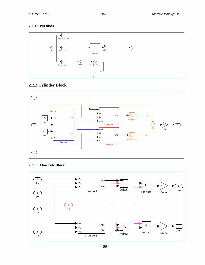
Master’s Thesis 2010 Mhretie Molalign M.
- 56 -
2.2.1.1 PID Block
2.2.2 Cylinder Block
2.2.1.1 Flow rate Block
1
y
SumD
Sum
P
Proportional Gain
1
s
Integrator
I
Integral Gain
N
Filter Coefficient
1
s
Filter
D
Derivative Gain
1
u
1
F1
Ps
ps
Pa
Ps
Xa
Pe
Pb
dma
dmb
flow rate
dmb
Pb
dx
x
dPb
chamberB
x
dx
Pa
dma
dPa
chamberA
Pe
Pe1
s
Integrator1
1
s
Integrator
-K-
Ap
3
u1
2
dq
1
q
2
dmb
1
dma
Pe
Ps
Pb
f AB
f BB
chamberB
Pa
Ps
Pe
f AA
f BA
chamberA
Switch1
Switch
Product1
Product
-K-
Gain1
-K-
Gain
5
Pb
4
Pe
3
Xa
2
Ps
1
Pa

Master’s Thesis 2010 Mhretie Molalign M.
- 57 -
2.2.1.2 Block Diagram for Chambers Under the Flow rate Block
2.2.2 Chamber Block Under Cylinder Block Diagram
2
fBA
1
fAA
Product1
Product
Pu
Pdf Prfcn
Embedded
MATLAB Function1
Pu
Pdf Prfcn
Embedded
MATLAB Function
-K-
1/sqrt(Ts)
-K-
1/sqrt(TS)
3
Pe
2
Ps
1
Pa
1
dPak
k
-K-
RTs/Ap
L/2
4
dma
3
Pa
2
dx
1
x

Master’s Thesis 2010 Mhretie Molalign M.
- 58 -
References
[1] Lui X-J., Wang Q-M. and Wang J. „‟Kinematic, Dynamic and Dimensional Synthesis of a
Novel 2 DoF Translational Manipulator‟‟. Journal of Intelligent and Robotic Systems 41, 205-
224, 2004
[2] Lui X., Wang J. and Pritschow G. „‟On the optimal kinematic design of a PRRRP 2-DoF
parallel mechanism‟‟. Mechanisms and Machine Theory 41, 1111-1130, 2006
[3] Wu J., Li T., Lui X. And Wang L. ‟‟Optimal kinematic design of a 2-DOF parallel
manipulator‟‟. Tsinghua Science and Technology 12(3), 269-275, 2007
[4] Sergiu-Dan S., Maties V. and Balan R. „‟ A multi criteria approach for the optimal design of 2
dof parallel robots used in construction applications‟‟.24th International Symposium on
Automation & Robotics in Construction, 2007
[5] Wang L-P., Wang J-S. and Chen J. „‟The dynamic analysis of a 2-PRR planar parallel
mechanism‟‟. Journal of Mechanical Engineering Science Vol. 219 Part C, 2005
[6] Sergiu-Dan S., Maties V. and Balan R. „‟ Multi-objective Design Optimization of Mini Parallel
Robots Using Genetic Algorithms‟‟. IEEE 1-4244-0755-9/0, 2007
[7] Wu J., Wang J., Li T. and Wang L.„‟ Analysis and Application of a 2-DOF Planar Parallel
Mechanism‟‟. ASME Journal of Mechanical design Vol. 129, April 2007
[8] Wang L-P., Wang J-S., Li Y-W. amd Lu Y. „‟ Kinematic and dynamic equations of a planar
parallel manipulator‟‟. Journal of Mechanical Engineering Science Vol.217 Part C, 2003
[9] Yui Y.K., Cheng H., Xiong Z.H., Liu G.F. and Li Z.X. „‟On the Dynamics of Parallel
Manipulators‟‟. Proceedings of the 2001 IEEE international Conference on Robotics &
Automation, May 21-26, 2001
[10] Sorli M., Gastaldi L., Codina E. and de la Heras S. „‟Dynamic analysis of pneumatic actuators‟‟.
Simulation Practice and Theory 7, 589-602, 1999
[11] Richer E. and Hurmuzlu Y. „‟a high performance pneumatic force actiator system: part I-

Master’s Thesis 2010 Mhretie Molalign M.
- 59 -
Nonlinear mathematical model‟‟. Journal of Dynamic Systems, Measurement, and Control Vol.
122, September 2000
[12] Kothapalli G. and Hassan Y. „‟Design of a Neural Network Based Intelligent PI Controller for a
Pneumatic System‟‟. IAENG International Journal of Computer Science, 35:2, 20 May 2008
[13] Blagojevic V. and Stojiljkovic M. „‟Mathematical and Simulink model of the pneumatic system
with bridging of the dual action cylinder chambers‟‟. FACTA UNIVERSITATIS: Mechanical
Engineering Vol.5 No1, pp 23-31, 2007
[14] Fok S.C. and Ong E.K. „‟ Position control and repeatability of a pneumatic rodless cylinder
continuous positioning‟‟, Robotics and Computer Integrated Manufacturing Vol. 15, 365-371,
1999
[15] Sobczyk S., Mario R. and Eduardo A. „‟Variable structure cascade control of a pneumatic
positioning system‟‟. ABCM Symposium Series in Mechatronics Vol.2, 27-34, 2006
[16] Chen C.K. and Hwang J. „‟Iterative learning control for position tracking of a pneumatic
actuated X–Y table‟‟. Control Engineering Practice 13, 1455-1461, 2005
[17] Yu S.J., Qi X.D., Han R.C. and Pan F. „‟Practical Design of an Iterative Learning-Sliding Mode
Controller for Electro-Pneumatic‟‟. International Journal of Information Technology Vol. 11no.
5
[18] Smaoui M., Brun X. and Thomasset D. „‟Systematic Control of an Electro-pneumatic System:
Integrator Backstepping and Sliding Mode Control‟‟. IEEE Transactions on control systems
technology, vol. 14, no. 5, september 2006
[19] Situm Z., Petric J. and Crnekovic M. „‟Sliding Mode Control Applied to Pneumatic Servo
Drive‟‟ Department of Automatic Control, Faculty of Mechanical Engineering and Naval
Architecture, University of Zagreb
[20] Wang J., Kotta U. and Ke J. „‟Tracking control of nonlinear pneumatic actuator systems using
static state feedback linearization of the input–output map‟‟. Proceeding of Estonian Academic
for Science Physics and Mathematics, Vol. 56, No. 1, 47–66, 2007

Master’s Thesis 2010 Mhretie Molalign M.
- 60 -
[21] Errahimi F., Cherrid H., Sirdi N.K.M. and Abarkane H. „‟ Robust adaptive control and observer
for a robot with pneumatic actuators‟‟. Cambridge University Press: Robotica Vol. 20, 167-173,
2002
[22] Spong M.W., Hutchison S. and Vidyasagar M. „‟Robot Modeling and Control‟‟. JOHN WILEY
& SONS, INC.
[23] Giberti H., Chatterton S. and Cinquemani S. „‟Kinematic Optimization of a Parallel Manipulator
5R 2-dof Driven by Pneumatic Cylinders‟‟. Dipartimento di Meccanica, Politecnico di Milano,
Italy
[24] Briot S. and Bonev I.A. „‟Are parallel robots more accurate than serial robots?‟‟ CSME
Transactions Vol 31, No 4, 445-456, 2007
[25] Shang W.W., Cong S. and Jiang S.L. „‟Dynamic model based nonlinear tracking control of a
planar parallel manipulator‟‟. Springer Science+Business Media, 2009
[26] Merlet J-P. „‟Solving the forward kinematics of a Gough-type parallel manipulator with interval
analysis‟‟. The International Journal of Robotics Research Vol. 23, No. 3, 221-235, March
2004
[27] Bardat C., Nabat V., Company O., Krut S. and Pierrot F. „‟Par2: a Spatial Mechanism for Fast
Planar, 2-dof, Pick-and-Place Applications‟‟. Proceedings of the Second International
Workshop on Fundamental Issues and Future Research Directions for Parallel Mechanisms
and Manipulators. September 21–22, 2008
[28] Huynh P., Arai T., Koyachi N. and Sendai T. „‟Optimal Velocity based control o parallel
manipulator with fixed linear actuators‟‟. IEEE:-Proc. IROS 97, 1997
[29] Wang Z., Wang Z., Liu W. and Lei Y. „‟A study on workspace, boundary workspace analysis
and workpiece positioning for parallel machine tools‟‟. Elsevier Science: Mechanisms and
Machine Theory Vol. 36, 605-622, 2001

Master’s Thesis 2010 Mhretie Molalign M.
- 61 -
[30] Ali H.I., Noor S.B.M., Bashi S.M. and Marhaban M.H. „‟A review of pneumatic actuators
(modeling and control)‟‟. Australian Journal of basic and applied Sciences Vol. 3(2), 440-454,
2009
[31] Najafi F., Fathi M. and Saadat M. „‟Dynamic modeling of servo pneumatic actuators with
cushioning‟‟. International Journal of Advanced Manufacturing Technologies Vol. 42, 757-765,
2009
[32] Khayati K., Bigras P. and Dessaint L.A. „‟Nonlinear control of pneumatic systems‟‟. École de
Technologie Supérieure,214-220,
[33] Richer E. and Hurmuzlu Y. „‟a high performance pneumatic force actiator system: part II-
Nonlinear control design‟‟. Journal of Dynamic Systems, Measurement, and Control Vol. 122,
September 2000
[34 Lee H.K., Choi G.S. and Choi G.H. „‟A study on tracking position control of pneumatic
actuators‟‟. Elsevier Science: Mechatronics Vol. 12, 813–831, 2002
[35] Llagostera H.M. „‟Control of a pneumatic servosystem using fuzzy logic‟‟ Proc. of 1st FPNI-
PhD Sym., pp. 189-20, 2000. Hamburg
[36] Papoutsidakis M.G., Chamilothoris G. and Pipe a. „‟Auto-Selective Three Term Control of
Position and Compliance of a Pneumatic Actuator‟‟. World Academy of Science, Engineering
and Technology 26, 2007
[37] Ilchemann A., Sawodny O. and Trenn S. „‟Pneumatic cylinders: modeling and feedback
force-control‟‟. Technische Universit¨at Ilmenau,2 May 2005
[38] Nouri B.M.Y., Al-Bender F., Swevers J., Vanherck P. and Van Brussel H. „‟Modeling a
pneumatic servo positioning system with friction‟‟. Preceedings of the American
control Conference, 2000, Chicago, Illinois
[39] Zhu X., Cao J., Tao G. and Yao B. „‟Synchronization Strategy Research of Pneumatic
Servo System Based on Separate Control of Meter-in and Meter-out‟‟. IEEE/ASME
International Conference on Advanced Intelligent Mechatronics, July 14-17, 2009

Master’s Thesis 2010 Mhretie Molalign M.
- 62 -
[40] Gelezevicius V. and Grigaitis A. „‟Research of Adaptive Force Control Loop of
Electropneumatic Acting System‟‟ Electronics and Electrical Engineering No 7(79) ,
2007
[41] Sandler Ben-Z. „‟Robotics: Designing the mechanisms for automated machinery‟‟,
Second edition, Academic Press, 1991
[42] Xie M. „‟Fundamentals of Robotics: Linking Perception to Action‟‟, Machine
Perception Artificial Intelligent Vol 54, World Scientific publishing Co. Pte. Ltd., 2003
[43] Gibilisco Stan, „‟Concise Encyclopedia of robotics‟‟, MacGraw-Hill, 2003
[44] FESTO, Rodless drive units DGP/DGPL
[45] FESTO, End position controllers SPC11, Peripherals overview
[46] Stan Sergiu-Dan (Dr.). „‟What is a Parallel Manipulator? „‟. Senior Lecture Notes,
Technical University of Cluj-Napoca Department of Mechanisms, Precision Mechanics
and
[47] Corke Peter I. ‘‟Robotics TOOLBOX for Matlab, release 6’’, CSIRO Manufacturing
Science and Technology, 2001.
[48] Wood G.D. and Kennedy D.C., „‟Simulation Mechanical Systems in Simulink with
SimMechanics‟‟, The MathWorks
[49] FESTO DGP/DGPL, Rodless double-acting pneumatic linear actuator, Rodless
Actuators Basic Version, Metric Series
[50] FESO, Proportional directional control valves MPYE, 5/3-way valve function

Master’s Thesis 2010 Mhretie Molalign M.
- 63 -