politecnico di milano · 2017-10-27 · compressor annulus boundary layer model in a through-flow...

POLITECNICO DI MILANOScuola di Ingegneria Industriale e dell’Informazione

Corso di Laurea in Ingegneria Aeronautica

Analysis and Implementation of an AxialCompressor Annulus Boundary Layer Model in a

Through-Flow Software

Relatore: Prof. Luigi VIGEVANOCo-relatore: Prof. Vassillios PACHIDIS

Tesi di laurea di:Riccardo GRETTER - Matr. 838520

Anno Accademico 2016-2017

To my family

AbstractIn this work, existing models for the development of the boundary layer onthe end walls of axial compressor are analysed.

Three solutions are taken into account for the bladed domain and areimplemented in a through flow code for the preliminary analysis of axialcompressor developed at Cranfield University, United Kingdom. Two so-lutions for the turbulent boundary layer development are validated withexperimental data and are used in the parts of the domain without blades.

The models are tested in fan geometries already present in the softwareand typical boundary layer quantities are compared with existing experimen-tal data. The geometry of a multistage axial compressor is then specificallyimplemented for further tests on a larger domain.

SommarioIn questo lavoro sono analizzati modelli per lo sviluppo dello strato limitesulle pareti di compressori assiali.

Tre soluzioni sono prese in considerazione per il dominio in cui sonopresenti palette e sono implementate in un codice through-flow per l’analisipreliminare di compressori assiali sviluppato presso Cranfield University,Regno Unito. Due soluzioni per lo sviluppo dello strato limite turbolentosono validate con dati sperimentali e sono usate nelle parti del dominio senzapalette.

I modelli sono testati in geometrie di fan già presenti nel software ele quantità tipiche dello strato limite sono comparate con i dati sperimen-tali esistenti. La geometria di un compressore assiale multistadio è poispecificatamente implementata per ulteriori test su un dominio più esteso.

I

Contents

1 Introduction 11.1 Motivation and Scope of Work . . . . . . . . . . . . . . . . . 31.2 Background to the Work . . . . . . . . . . . . . . . . . . . . . 41.3 Layout of the Thesis . . . . . . . . . . . . . . . . . . . . . . . 7

2 Literature Review 8

3 The Through-Flow code 183.1 How it works . . . . . . . . . . . . . . . . . . . . . . . . . . . 183.2 Operation . . . . . . . . . . . . . . . . . . . . . . . . . . . . . 193.3 Viscous Models . . . . . . . . . . . . . . . . . . . . . . . . . . 20

4 Boundary Layers in Adverse Pressure Gradient 224.1 Integral Solution . . . . . . . . . . . . . . . . . . . . . . . . . 224.2 Jansen Model . . . . . . . . . . . . . . . . . . . . . . . . . . . 234.3 Test 1: Flow 2200 . . . . . . . . . . . . . . . . . . . . . . . . 244.4 Test 2: Flow 2300 . . . . . . . . . . . . . . . . . . . . . . . . 274.5 Test 3: Flow 4000 . . . . . . . . . . . . . . . . . . . . . . . . 294.6 Discussion . . . . . . . . . . . . . . . . . . . . . . . . . . . . . 31

5 Annulus Boundary Layer Models 325.1 Boundary Layer Equations . . . . . . . . . . . . . . . . . . . 325.2 De Ruyck’s and Hirsch’s Correlation . . . . . . . . . . . . . . 335.3 Modified Aungier’s Model . . . . . . . . . . . . . . . . . . . . 355.4 Blockage . . . . . . . . . . . . . . . . . . . . . . . . . . . . . . 385.5 Critics to the models . . . . . . . . . . . . . . . . . . . . . . . 385.6 Implementation . . . . . . . . . . . . . . . . . . . . . . . . . . 39

6 Test on Available Geometries 436.1 Description . . . . . . . . . . . . . . . . . . . . . . . . . . . . 436.2 Experiments . . . . . . . . . . . . . . . . . . . . . . . . . . . . 456.3 Modelling . . . . . . . . . . . . . . . . . . . . . . . . . . . . . 456.4 Comparison with Experimental Boundary Quantities . . . . . 486.5 Results . . . . . . . . . . . . . . . . . . . . . . . . . . . . . . . 54

II

6.6 Discussion . . . . . . . . . . . . . . . . . . . . . . . . . . . . . 59

7 Test on Multistage Geometry 627.1 Description . . . . . . . . . . . . . . . . . . . . . . . . . . . . 627.2 Experiments . . . . . . . . . . . . . . . . . . . . . . . . . . . . 637.3 Modelling . . . . . . . . . . . . . . . . . . . . . . . . . . . . . 647.4 Results . . . . . . . . . . . . . . . . . . . . . . . . . . . . . . . 667.5 Discussion . . . . . . . . . . . . . . . . . . . . . . . . . . . . . 68

8 Conclusions and recommendation for further work 71

Bibliography 73

III

List of Figures

1.1 The Trent 1000 from Rolls Royce Plc: a modern turbofanengine. [54] . . . . . . . . . . . . . . . . . . . . . . . . . . . 1

1.2 The schematic representation of an axial compressor. [9] . . 21.3 Qualitative representation of some viscous effects in a rotor

passage. As it is apparent, the end wall boundary layer inturbomachines is a complicated highly three dimensional flow.[34] . . . . . . . . . . . . . . . . . . . . . . . . . . . . . . . . 3

1.4 Typical magnitude of losses on efficiency. [11] . . . . . . . . 41.5 Natural reference system and its relation with the cylindrical

coordinates (here the axial direction is named z). [9] . . . . 6

2.1 Plot of defect layers: displacement thickness and tangentialforce defect. [7] . . . . . . . . . . . . . . . . . . . . . . . . . 9

2.2 Ratio of displacement thickness and tangential force defectover pressure ratio. The force defect is seen to be a consistentpercentage of the displacement thickness. [7] . . . . . . . . . 9

2.3 Velocity profile along a 12 stage. [7] . . . . . . . . . . . . . . 102.4 Correlation for tangential force defect.[9] . . . . . . . . . . . 112.5 Velocity defect through a single rotor with artificially thickened

boundary layer, at different loading conditions. The thinningof the layer across the layer is apparent: this is the smallclearance case. [35] . . . . . . . . . . . . . . . . . . . . . . . 12

2.6 Displacement thickness along a 4 stages research compressor,the trends are clearly visible. [15] . . . . . . . . . . . . . . . . 13

2.7 Data for a 4 stages compressor from Smith (1969) reworkedfrom Horlock and Perkins [1]. . . . . . . . . . . . . . . . . . 13

2.8 Defects over pressure rise ratio. [34] . . . . . . . . . . . . . . 142.9 Computed boundary layer growth near to design mass flow

(5) and near stall (6). [46] . . . . . . . . . . . . . . . . . . . 152.10 Correlation of Khalid [18] with overimposed data of a tran-

sonic rotor from Suder [38]. . . . . . . . . . . . . . . . . . . 16

3.1 Initial screenshot of SOCRATES. . . . . . . . . . . . . . . . 19

IV

3.2 Example of the Blade Geometrical Data (input file four) forone rotor. . . . . . . . . . . . . . . . . . . . . . . . . . . . . . 20

3.3 Block scheme of the through-flow code and its implementedsubroutines for viscous effects. The whole procedure is re-peated a number I of "Timesteps" in which I different boundaryconditions are imposed. . . . . . . . . . . . . . . . . . . . . . 21

4.1 Tabulated velocity and polynomial interpolation used (4thorder). . . . . . . . . . . . . . . . . . . . . . . . . . . . . . . . 25

4.2 Displacement thickness computed using Euler and RungeKutta and Jansen’s model on original and interpolated datacompared with experimental data. . . . . . . . . . . . . . . . 25

4.3 Momentum thickness computed using Euler and Runge Kuttaand Jansen’s model on original and interpolated data com-pared with experimental data. . . . . . . . . . . . . . . . . . . 26

4.4 Friction coefficient computed using Euler and Runge Kutta,compared with experimental data. . . . . . . . . . . . . . . . 26




4.8 Friction coefficient computed using Euler and Runge Kutta,compared with experimental data. . . . . . . . . . . . . . . . 29




V

5.1 Comparison table for the maximum value of the norm of thecomputed displacement thickness and the delta between theinitialised value and the computed value at inlet and outletand at hub and tip of all turbocomponents. Each column isrelative to a model, in order: Jansen, Aungier with integralsolution, Correlation, Aungier with Jansen, Correlation withJansen. The highlighted column (Jansen model) clearly showsthe largest value in both absolute value and delta. The 1*colums indicates the results from the Jansen model scaledby a factor 0.5. The "result" row indicates whether the codeaccepted or not the first introduction of the computed valueand not whether the code converged or not. To note the firstapplication of the security switch at the tip for the cases withcorrelation: the delta with respect to initialisation is zerobecause the former value was kept. . . . . . . . . . . . . . . 41

6.1 The Rotor 67. [53] . . . . . . . . . . . . . . . . . . . . . . . 446.2 The flowpath of the TP 1493 with the position of the 3 mea-

suring station. The higher-aspect-ratio rotor of the previousdesign is also sketched. [42] . . . . . . . . . . . . . . . . . . 44

6.3 The geometry and grid solution for the NASA Rotor 67 insingle rotor configuration. . . . . . . . . . . . . . . . . . . . . 46

6.4 The geometry and grid solution for the NASA TP 1493. . . . 476.5 The flowpath of the TP 1493 with the position of the 5 mea-

suring station. [47] . . . . . . . . . . . . . . . . . . . . . . . 486.6 The experimental data from [47] compared with the results

at 50 percent of speed of the Aungier model with integralsolution in the domain without blades. . . . . . . . . . . . . 50

6.7 The experimental data from [47] compared with the resultsat 50 percent of speed of the Aungier model with Jansenmodel upstream and integral solution downstream the bladeddomain. [47] . . . . . . . . . . . . . . . . . . . . . . . . . . . 50

6.8 The experimental data from [47] compared with the results at50 percent of speed of the Jansen’s model, run in background. 51

6.9 The experimental data from [47] compared with the resultsat 50 percent of speed of the correlation with integral solutionin the domain without blades, run in background. [47] . . . 51

6.10 The experimental data from [47] compared with the resultsat 50 percent of speed and at 100 of speed of the Aungiermodel with a linear growth upstream and the integral solutiondownstream of the bladed domain. . . . . . . . . . . . . . . . 53

VI

6.11 Compressor map of the NASA Rotor 67 in single rotor con-figuration compared with experimental results, the boundarylayer is initialised and kept constant. The computed lines arecoloured. . . . . . . . . . . . . . . . . . . . . . . . . . . . . . 54

6.12 Compressor map of the NASA TP 1493 with experimentalresults, the boundary layer is initialised and kept constant.The computed lines are coloured. . . . . . . . . . . . . . . . 55

6.13 The computed map for 50 percent of speed for the single rotor:the case with no boundary layer model inserted is comparedwith the converged solutions with the model. . . . . . . . . . 55




6.17 The computed map for 100 percent of speed for the singlerotor: the case with no boundary layer model inserted iscompared with the converged solutions with the model. . . . 57

6.18 The computed map for 50 percent of speed for the complete fan:the case with no boundary layer model inserted is comparedwith the converged solutions with the model. . . . . . . . . . 58

6.19 The computed map for 70 percent of speed for the complete fan:the case with no boundary layer model inserted is comparedwith the converged solutions with the model. . . . . . . . . . 58

6.20 Defects over pressure rise ratio. [34] . . . . . . . . . . . . . . 596.21 Compressor map of the NASA Rotor 67 in single rotor configu-

ration compared with experimental results, the boundary layeris computed by the Aungier’s model with integral solution inthe not bladed domain. . . . . . . . . . . . . . . . . . . . . . 60

6.22 Compressor map of the NASA Rotor 67 in single rotor configu-ration compared with experimental results, the boundary layeris computed by the Aungier’s model with linear distributionupstream and integral solution downstream the bladed domain. 60

6.23 Compressor map of the NASA TP 1493 compared with ex-perimental results, the boundary layer is computed by theAungier’s model with linear distribution upstream and integralsolution downstream the bladed domain. . . . . . . . . . . . 61

7.1 Geometry of the NACA 5-stage. . . . . . . . . . . . . . . . . 637.2 The geometry and grid solution for the NACA 5-stage. . . . . 65

VII

7.3 Converged operating points compared to the experimentalcompressor map of the NACA 5-stage. . . . . . . . . . . . . 66

7.4 The computed map for 50 percent of speed for the NACA5-stage: the case with no boundary layer model inserted iscompared with the converged solutions with the model. . . . 67



7.7 Comparison of the computed boundary layer at hub at 70percent of speed for the two models at 20 kg/s and 19.2 kg/s. 69

7.8 Comparison of the computed boundary layer at tip at 70percent of speed for the two models at 20 kg/s and 19.2 kg/s. 69

7.9 Comparison of the computed boundary layer at hub at 70percent and at 80 percent of speed for Aungiers’s model. . . 69

7.10 Comparison of the computed boundary layer at tip at 70percent and at 80 percent of speed for Aungiers’s model. . . 70

VIII

AcronymsCAD Computer Aided Design

CFD Computational Fluid Dynamics

DCA Double Circular Arc

EGV Exit Guide Vane

IGV Inlet Guide Vane

LES Large Eddy Simulation

MCA Multiple Circular Arc

RANS Reynolds Averaged Navier Stokes

SLC Streamline Curvature

REE Radial Equilibrium Equation

SOCRATES Synthesis Of Correlations for the Rapid Analysis ofTurbomachine Engine Systems

IX

Chapter 1

Introduction

In Figure 1.1 is shown a modern aero engine from Rolls Royce Plc, the Trent1000. It has an overall compressor ratio of 50:1 and it generates up to 340 kNof thrust. It is a three shaft turbofan with a single rotor inlet fan, a 8-stageintermediate pressure compressor and a 6-stage high pressure compressor.The bypass ratio, i.e. the ratio of the mass flow through the fan over themass flow through the core compressor is higher than 10:1. In Figure 1.2 ispresented a schematic representation of an axial compressor. The endwall atcasing and hub is indicated.

The annulus boundary layer in axial compressors is different from theboundary layers on wings or within ducts in the fact that it is extremelynot well behaved. The hub and casing boundaries of the turbomachinewill themselvevs contain steps and gaps separating moving and stationary

Figure 1.1: The Trent 1000 from Rolls Royce Plc: a modern turbofan engine. [54]

1

Figure 1.2: The schematic representation of an axial compressor. [9]

components, resulting in a segmented wall with relative motion from seg-ment to segment. The end wall boundary layer spans these interruptionsand it is intermittently subjected to centrifugal and Coriolis forces. Thesecomplications are nevertheless minor when one considers the effects of bladerows. The deflection of the end wall shear layer by a cascade of blades givesrise to secondary flows which are often greater in intensity and scale thanthe conventional transport motions of the boundary layer. In addition, thestrong outward migration of low velocity fluids gives often rise to severe wakelike velocity defects at some distance from the wall. Ultimately, in presenceof unshrouded blade tips a complex large scale vortex motion adds a finalcomplication [1]. In Figure 1.3 a sketch shows some of the relevant viscouseffects within a rotor passage. In particular, to summarize the effects thatmust be taken into account when modelling a flow of this complexity, thecomplex highly three-dimensional effects that must be considered are:

• inlet skew;

• force, displacement and momentum defects;

• secondary recirculation in passage;

• turbolent mixing;

• hub-suction vortex;

• leakage flows;

• etc..

Such flow can be analysed through complete 3D CFD tools, by solvingReynolds Averaged Navier-Stokes equations (RANS) or even employing LargeEddy Simulations (LES). Proper models for turbulence are able to resolve

2

Figure 1.3: Qualitative representation of some viscous effects in a rotor passage.As it is apparent, the end wall boundary layer in turbomachines is acomplicated highly three dimensional flow. [34]

all these flow effects. Nevertheless, they are still extremely computationallyexpensive when dealing with complex geometries such as multi-stage axialcompressors and therefore not suitable in a preliminary design phase wherethe many degrees of freedom must be considered to obtain an optimumtrade-off and maximize efficiency. Here is where computational tools such asthe one employed in this work prove their effectiveness.

1.1 Motivation and Scope of WorkThe annulus boundary layers have a small effect on blade row turning orstage work, but a very large effect on efficiency at design and off-design flowrates and wheel speeds. In the Figure 1.4 from Balsa and Mellor it is possibleto appreciate the typical stage performance with or without the inclusion ofthe annulus boundary layer. In particular, the scope of work of this Thesisis to analyse and test different annulus boundary layer models suitable for atime efficient through-flow computations and to implement them in a code,in-house developed at Cranfield Univesity. In order to do so, the literatureabout the subject has been deeply analysed and some possible models ofincreasing complexity have been selected. The models have then been testedfor different geometrical configurations, already descibed in the software. Inaddition, the geometry of a larger compressor has also been implemented inorder to gain a more complete overview on the capabilities of the models.

3

Figure 1.4: Typical magnitude of losses on efficiency. [11]

1.2 Background to the WorkWhen dealing with boundary layers, it is costumary to define the defectquantities. The concept developed by Schlichting and Prandtl at the begin-ning of last century, of dividing the freestream flow from the flow near to awall had a great success and it is still in use today. In the freestream flowis possible to simplify the Navier-Stokes equations, obtaining the inviscidEuler equations. The concept is the use of integral quantities: renouncing torepresent the velocity profile in direction normal to the wall and integratingin that direction to obtain a quantity called "defect quantity". In other wordsthe dimensionality of the problem is reduced of 1. This is what is classicallydone when defining the displacement thickness and the momentum thickness.They are defined, in a 2D reference system with the x-axis along the physicalboundary and the y axis normal to it, as:

ρeVeδ∗ =

∫ δ

0(ρeVe − ρV ) dy

ρeV2e θ =

∫ δ

0ρV (Ve − V ) dy

And the shape factor will be the ratio of the two:

H = δ∗

θ

4

In this definitions, displacement thickness is represented by δ∗ and momentumthickness by θ, ρ is the density and V the velocity. The subscript e indicates"external", the quantities without subscript are relative to the boundary layeritself, and the integral is taken on δ, which is the boundary layer thickness(thickness 6= displacement thickness). Normally the shape factor will bein the range 1 < H < 2.2 and 2.2 or 2.4 are commonly referred to as thelimit shape factors before flow separation. To understand this concept it iseasy to think that the flow will separe when the boundary layer geometry(displacement) will be too large for the energy it contains (momentum). Sincein this work is dealt with boundary layers inside a turbomachine, it is alsofundamental to describe which are the main reference systems and whichadditional defects need to be introduced. When dealing with turbomachines,two main reference planes are usually employed: the meridional plane and theblade-to-blade plane. If the axial direction is set along the main longitudinalaxis of the machine and the radius is computed as the distance from this mainlongitudinal axis on a normal plane, then the meridional plane is definedas the (x,r) plane. In other words, the meridional plane is a slice of theturbomachine on a fixed θ, where θ will be an angle on the plane normalto the main longitudinal axis of the machine. The meridional plane for aschematic compressor can be seen in Figure 1.2. The blade-to-blade plane,instead, can be imagined as something that cuts the blades while turningaround the main axis at a fixed radius. In other words, it is the plane (θ,r). It is normal anyway not to use cilindrical coordinates (x, r, θ) to definethe directions in a turbomachine, but to use the "natural" reference system(m,n, θ). This reference system is easily derived from the previous. m isusually very close to the axial direction x, but it is tangent to a streamlinepassing through the turbomachine. A streamline is defined as a curve in themeridional plane having no fluid velocity normal to it. The angle between mand x is usually referred to as the streamline slope and called with the greeksymbol φ. The second direction, n, is the normal to m, in the meridionalplane, while the last direction, t or θ is the normal to the meridional plane.Figure 1.5 shows graphically the natural reference system related with thestandard cylindrical system.

For what concerns the defects, in a turbomachine it is mandatory toconsider a three dimensional boundary layer. As briefly mentioned before, theflow it is extremely bad behaved and it could not be treated as if it was twodimensional (even though this is ultimately done). In this sense the quantitiesthat must be defined are, in order: the meridional displacement thickness,the meridional momentum thickness, the mixed momentum thickness, thetangential displacement thickness, the tangential momentum thickness:

ρeVmeδ∗1 =

∫ δ

0(ρeVme − ρVm) dn

5

Figure 1.5: Natural reference system and its relation with the cylindrical coordinates(here the axial direction is named z). [9]

ρeV2meθ11 =

∫ δ

0ρVm(Vme − Vm) dn

ρeVmeVθeθ12 =∫ δ

0ρVm(Vθe − Vθ) dn

ρeVθeδ∗2 =

∫ δ

0(ρeVθe − ρVθ) dn

ρeV2θeθ22 =

∫ δ

0ρV (Vθe − Vθ) dn

In these definitions the subscripts m stays for "meridional" and the subscriptθ stays for "tangential". The subcript 11, 12, and 22 indicate respectivelythe boundary quantity in the meridional direction, in a "mixed" direction(see definition, it considers velocities along m and along θ) and in thetangential direction. Furthermore, as will be explained in Chapter 2, anotherfundamental quantity for the boundary layer in turbomachines is the forcedefect. The force defect is defined in the same way as the displacementthickness or the momentum thickness and it describes how the force of theblade decreases when it is immersed in the boundary layer. It is defined intwo directions, accordigly to the reference system just described (meridionaland tangential):

νmfme =∫ δ

0(fme − fm) dn

νθfθe =∫ δ

0(fθe − fθ) dn.

In these definitions ν is the force defect and f the force of the blade (perunit volume). When introducing these defect quantities inside the equationof motion, these are normally integrated both along the boundary layer

6

thickness δ and along the pitch in tangential direction. The pitch is thedistance between one blade ad the following in tangential direction, i.e. theblade passage.

1.3 Layout of the ThesisThe Thesis will be articulated as follows. A first description of the overallliterature backgroud about the subject of annulus boundary layer is firstpresented (Chapter 2). Then, the through-flow code which will representthe environment where the model will act is exposed in Chapter 3. In orderto apply the model, two main domains are identified: in Chapter 4 possiblesolutions for the parts of the domain without blade rows are investigatedwhile in Chapter 5 are described and critically analysed some of the modelsfor the bladed domain extracted from the literature. Herein, their limitsand the design choices for the implementation are underlined. Results ofthe performances of the models are finally described in the two followingchapters: in Chapter 6 some geometries already available in the softwareare experimented and in Chapter 7 a more suitable compressor geometryhas been appositely loaded, validated and run. Discussion and proposal forfurther work conclude the Thesis in Chapter 8.

7

Chapter 2

Literature Review

When looking at the complexity of the flow, the need for a compromise isself-evident. In the first approaches to predict compressor performances, theboundary layer was not computed but determined values of blockage wereassigned, accordingly to experience with known compressor designs, with alinear variation along the axis, or linear variation in early stages and constantvalues in rear stages [2], [3].

The first attempts to compute boundary layers properties in compressorsusing boundary layer techniques are attributed to Stratford [4] and Jansen[5] in 1967. In both methods the problem is simplified to a bidimensionalequation for the axial growth of the boundary layer momentum thickness,which is decoupled from the transverse momentum thickness equation. WhileStratford employed a flat plate approximation for the boundary layer shapefactor and wall stress, Jansen used an approximated integral solution from theclassical work of Schlichting [6]. Further studies showed that these analyseswere oversimplified, but they are relevant in their introduction of the study ofthe problem using pitch averaged boundary layer quantities. An interestingpart of the work of Stratford is its application of the axial momentum balanceto show the link between the momentum thickness growth and the forcedefect. In particular, by considering a control volume in two dimensions fromstation 1 to station 2 and applying the conservation of axial momentum [4]:

fxνx = ρ(V 2x2θx2 − V 2

x1θx1 + (Vx2 − Vx1)Vx2δ∗x2

)(2.1)

Where f is the blade force per unit surface, ν is the force defect, θ themomentum thickness, ρ the density, V the axial component of velocity,the subscript x indicates the axial direction and the subscripts 1 and 2indicate the inlet and outlet stations. Physically the axial boundary layerflow could never surmont the pressure rise if the latter wasn’t almost entirelycovered by the blade force (normal turbolent boundary layers separe at apressure difference of ∆P = 0.6(ρV 2

x /2) while in a compressor is normal tohave ∆P = 2.3(ρV 2

x /2) ). For many applications one can assume that the

8

Figure 2.1: Plot of defect layers: displacement thickness and tangential force defect.[7]

(a) At the casing. (b) At the hub.

Figure 2.2: Ratio of displacement thickness and tangential force defect over pressureratio. The force defect is seen to be a consistent percentage of thedisplacement thickness. [7]

velocites outside the boundary layer be similar (Vx1 ≈ Vx2) and therefore theequivalence is simplified:

fxνx = ρV 2x (θx2 − θx1) (2.2)

Which heuristically shows that momentum thickness and defect force arelinked. This is also shown in the work of Smith [7], which will be mentionedseveral times. In particular from the pictures (Figure 2.1 and Figure 2.2) itcan be seen how the displacement thickness and the force defect are clearlylinked, even if a correlation is not easy to find.

Sadly, there aren’t many other experimental comparable results aboutthe growth of the boundary layer in axial compressors (a great effort hasbeen dedicated particularly to the flow dynamics of blade cascades, which

9

Figure 2.3: Velocity profile along a 12 stage. [7]

have then been proved to be different from the compressor results for anumber of factors [34]). The reason for this lack of information is due tothe expensive set up and working cycles inherent at the use of a researchcompressor. In fact, most on the research devoted to compressor has beencarried out with the support of some large aircraft engine productors. Thealready mentioned experimental result provided by Smith in his analysis ofa 4 stage and 12 stage compressor (see Figure 2.3) shows particularly howthe blade forces can not be assumed constant though the defect layer, howwas firstly assumed by Stratford.

The experimental verification of Smith also supports the repeating stagemodel, according to which after several stages (two or three [34]) the bound-ary layer will reach an equilibrium position and won’t change anymore. Atthis point the growth is seen as a function of the blade loading.

In a later publication the same Smith and Koch [8] will provide whatis, accordingly to Aungier [9], the best available experimental base for thetangential force defects. The data is extremely scattered and a correlationdoesn’t appear to be useful, but with a different normalisation provided byAungier, the situation is slightly improved. These are the data which arelater employed in the implementation of one of the models (Figure 2.4).

The problem of providing a theoretical base for the boundary layer devel-opment within axial compressors has been addressed by Mellor and Wood in1971 [10] and later by Balsa and Mellor in 1975 [11], who derived the completethree dimensional equations (integrated over the boundary layer thickness δand the pitch (distance between one blade and the following in a tangentialdirection, i.e. the blade passage)) and some reasonable models for everydefect quantity. This development includes effects previously neglected suchas blade forces defects and jump conditions between rotating and stationaryblade rows. A model for secondary flow was built in order to seriously treatthe difference between tangential and meridional momentum thicknesses andit was assumed that the overall blade force remains approximately normal

10

to the mean freestream vector. In this way the idea of the repeating stagecondition was kept valid. Even if it clearly was an improvement with respectto the past, this first theory still suffered of many problems: for exampleshape factor and skin friction coefficient were somehow arbitrarily assigned tomatch experimental data in overall compressor performance prediction. Builtupon the theoretical base provided, Hirsch [12] and De Ruyck and Hirsch[13], [14] published a series of articles regarding the further developmentof the models and the application on a numerical solver. Here they discussin greater detail the terms of the force defect and study different optionsfor it, including several correction of the previous work. They also proposea correlation as a function of a number of geometrical and flow properties,based on the assumption of an equilibrium condition.

Later on, it is critical to mention the important experimental work ofCumpsty and Hunter [35] and later Cumpsty [15]. Their work on a singlerotor is significant because it experimentally shows the importance of thetip clearance. The tip clearance is the spacing between the tip of the bladeand the end wall. In the paper of Cumpsty and Hunter is provided a tablewith the displacement thickness before and after the rotor, at different inletboundary conditions. The layer is first observed to thin across the rotor whenthe tip clearance is 1 percent of the blade chord (see Figure 2.5), while a laterincrease of tip clearance is clearly seen to increase the displacement thicknessdownstream the rotor, de facto inverting the previuosly observed behaviourand making the clearance a fundamental parameter for the determination ofthe boundary layer thickness (this was already established by the theoreticaland experimental work of Lakshminarayana about the tip region flow physicsand its effects on the boundary layer development [16], [37]). This suggested

Figure 2.4: Correlation for tangential force defect.[9]

11

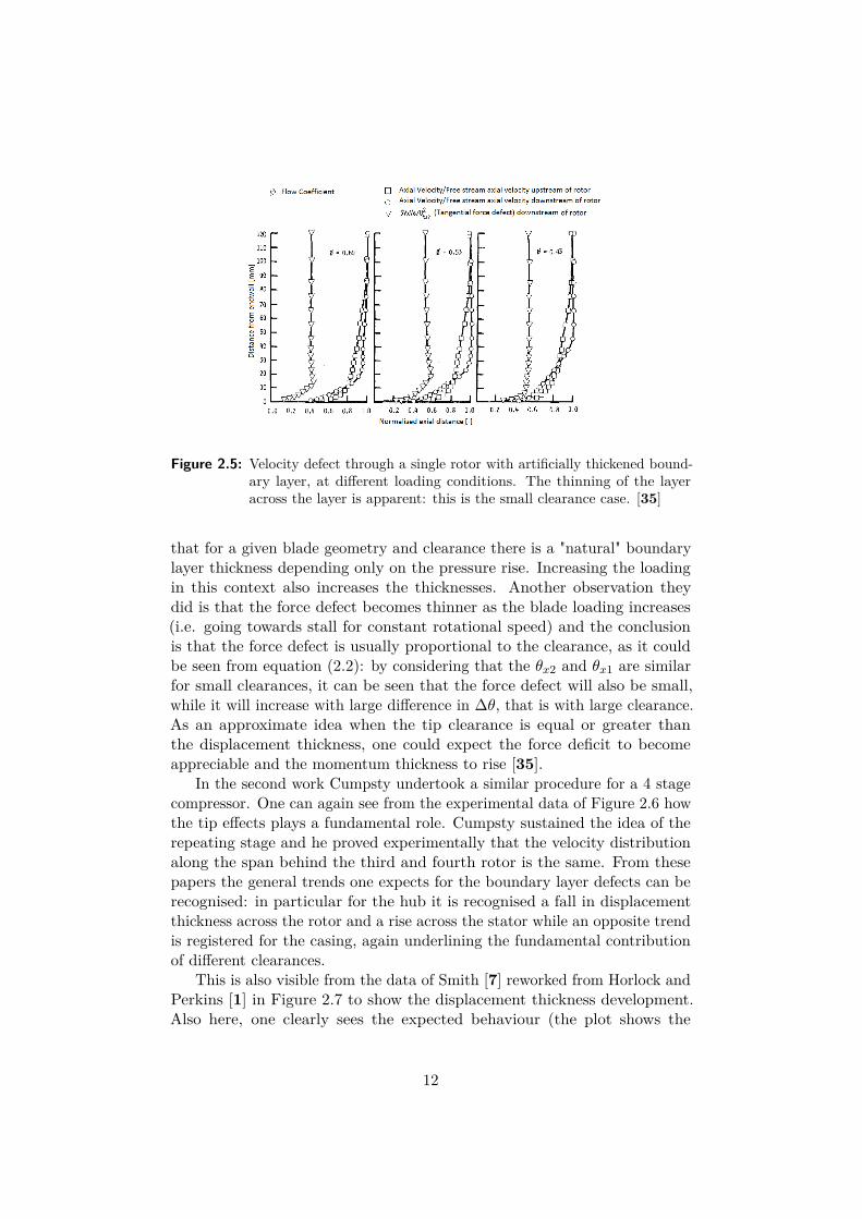
Figure 2.5: Velocity defect through a single rotor with artificially thickened bound-ary layer, at different loading conditions. The thinning of the layeracross the layer is apparent: this is the small clearance case. [35]

that for a given blade geometry and clearance there is a "natural" boundarylayer thickness depending only on the pressure rise. Increasing the loadingin this context also increases the thicknesses. Another observation theydid is that the force defect becomes thinner as the blade loading increases(i.e. going towards stall for constant rotational speed) and the conclusionis that the force defect is usually proportional to the clearance, as it couldbe seen from equation (2.2): by considering that the θx2 and θx1 are similarfor small clearances, it can be seen that the force defect will also be small,while it will increase with large difference in ∆θ, that is with large clearance.As an approximate idea when the tip clearance is equal or greater thanthe displacement thickness, one could expect the force deficit to becomeappreciable and the momentum thickness to rise [35].

In the second work Cumpsty undertook a similar procedure for a 4 stagecompressor. One can again see from the experimental data of Figure 2.6 howthe tip effects plays a fundamental role. Cumpsty sustained the idea of therepeating stage and he proved experimentally that the velocity distributionalong the span behind the third and fourth rotor is the same. From thesepapers the general trends one expects for the boundary layer defects can berecognised: in particular for the hub it is recognised a fall in displacementthickness across the rotor and a rise across the stator while an opposite trendis registered for the casing, again underlining the fundamental contributionof different clearances.

This is also visible from the data of Smith [7] reworked from Horlock andPerkins [1] in Figure 2.7 to show the displacement thickness development.Also here, one clearly sees the expected behaviour (the plot shows the

12

Figure 2.6: Displacement thickness along a 4 stages research compressor, the trendsare clearly visible. [15]

combined effect of hub and tip: the tip effect is supposed to be the mostimportant and therefore the reduction of the displacement thickness isthrough stators and the increase through rotors).

It is relevant that the data of the work of Cumpsty and Hunter of 1982 fora single rotor collapse on the same curve as the experimental data of Smithand Koch in 1970 for a 4-stage compressor, already mentioned, when plottedagainst the ratio of effective versus maximum pressure increase and with adifferent normalisation, for both tangential force defect and displacement

Figure 2.7: Data for a 4 stages compressor from Smith (1969) reworked from Horlockand Perkins [1].

13

(a) Displacement thickness.

(b) Tangential force defect.

Figure 2.8: Defects over pressure rise ratio. [34]

thickness. This is visible in Figure 2.8. Accordingly to Cumpsty, thisrepresents the best available experimental base for the tangential forcedefects [34].

The tangential force defect is relevant in a different way with respect tothe axial force defect. The latter is useful to calculate the axial displacementthickness and therefore the blockage, the former has the same meaning for thetangential defects and it also modifies the efficiency of the compressor. Thelarger the force defect, the less will be the torque needed by the compressorand the greater will be the efficiency. From the formula developed fromSmith [7] the efficiency results:

η = η1− (δh + δt)/h1− (νh + νt)/h

With η the efficiency without these effects, h the blade span, δ thedisplacement thicknesses and ν the tangential force defects at hub and tip(subscripts h and t respectively). In the Figure 1.4 in the Introduction isgraphically shown the same concept of relevant efficiency drop.

Another work on a 4-stages compressor carried on for the AGARD 175in 1981 yields interesting results for the effect of mass flow variation over theboundary layer development [46]. It is shown for the given rotating speed, ascould be expected, that the decrease of mass flow to near stall level results ina thickening of the boundary layer (of the order of 20% more between designcondition and near to stall condition). The results showed in the next Figure2.9 are based on the Mellor and Wood model, accurately tuned. They areconsidered reliable in function of the good correlation among the computedperformance results and the experimental performance data.

14

Figure 2.9: Computed boundary layer growth near to design mass flow (5) andnear stall (6). [46]

In the 90es are notable the work of Dunham in 1993 [17] and laterthe work of Khalid in 1994 [18] and Khalid et al. in 1999 [19]. Thework of Dunham is a further development of the theory as it was proposedby De Ruyck and Hirsch, in which models for the tip clearance vorticityand secondary flow are added that allow a better representation of thetip clearance effects and different expressions for the force defects are alsoproposed. The improvement is nevertheless limited and in the same yearDenton states that "it is hard to believe that anything other than 3D Navier-Stokes computations can give general results" [36]. Khalid instead in his Phdthesis proposed a different approach that considers an inviscid tip clearancemodel and an interesting correlation between pressure gradients and blockagefactor that, when suitabily normalized, makes all considered data collapseon a unique curve. His work is further developed in the paper of 1999, inwhich a tentative for a sistematic solution of the boundary layer problem isproposed. The procedure for defining blockage is firstly defined on the basisof a simplified model built on the previous work (on pressure gradients) andthen influencial geometrical parameter are found. In 1998 Suder [38] tried touse his correlation for a single rotor, the NASA Rotor 37, with results whichalso collapsed on the same curve (see Figure 2.10). The problem with thisapproach in the current analysis is that the model makes use of the pressurevariation across a blade row normalized on the pressure variation across theblade tip, which is a parameter which is not available from a through-flowcomputation.

From 2000 the method proposed by Aungier [9] for the boundary layercalculation based on the theoretical base provided by Mellor and Balsa and

15

on the experimental data of Smith and Koch, mentioned previously, hasbeen carefully studied. This method is developed in both meridional andtangential direction and with a number of assumptions provides an iterativesolution of the boundary layer equations which appears to be promising forthe application on a through-flow code and will be throughly exposed in thefollowing. Aungier’s method is further modified in 2015 and adapted onlyin two dimensions to reduce the number of assumptions and focus on themost interesting result for practical applications in a through-flow code: thecalculation of the blockage factors along the domain [22], [23]. The resultsappeared promising.

Interesting to understand the features and the complexity of the flow, wasthe serie of articles of Gdabebo [20], [21]. He used concepts of topology toexplain and describe the features of the three dimensional hub-suction surfaceseparation in a blade cascade, clearly visible from experimental verificationand the use of a 3D Navier-Stokes solver. The work confirms the intrinsicdifferences in the 3D separation and 3D flow behaviour with respect to thestandard 2D computations and underlines the limitations of a bidimensionalapproach on such complex geometries.

Realistically and to conclude, there is no current reliable method tocompute the annulus boundary layer in a compressor using the concept ofintegral solutions. Semi-empirical methods such the ones described above canbe implemented in some form for through-flow codes for the rapid preliminary

Figure 2.10: Correlation of Khalid [18] with overimposed data of a transonic rotorfrom Suder [38].

16

analysis of a number of possible designs, but the tendency is then to solvemore precisely the problem implementing 3D CFD codes which are able tocapture the smallest flow scales on different geometries [24].

17

Chapter 3

The Through-Flow code

In this chapter the code on which the work was performed is briefly describedin its basic assumptions and its operation. The code where the model has beenimplemented is a Streamline Curvature Method (SLC) developed by Pachidisand Templatexis in 2006 [25], [26] and called SOCRATES (Synthesis OfCorrelations for the Rapid Analysis of Turbomachine Engine Systems). Thetheoretical background on which this method is built comes from the paperof Wu in 1952, according to which the equations of the flow field are satisfiedand solved on two intersecting families of stream surfaces [27]. The programis written in Fortran. It is currently employed for the preliminary designphase of axial compressors in projects carried out by Cranfield Universitywith Rolls Royce Plc and other companies.

3.1 How it worksThe assumptions when one considers SLC are of steady, inviscid, adiabaticand axisymmetric flow. The equation being solved, which can be found in[29], is the so called REE (Radial Equilibrium Equation): it is a secondorder equation for velocity that summarises the momentum, state and energyequations. The solution scheme is a dynamic procedure appositely developedfor this application and it is accurately described in [45]. The method solvesthis discretized equation on a computational domain constructed in themeridional plane and bounded by the compressor annulus geometry. Gridnodes are defined at the intersections of the streamlines and blade edges.At the beginnning, the coordinates of the nodes are not known becausethe position of each streamline has not been defined yet. After one initialguess, new position of the nodes can be determined and the equations areintegrated from the compressor inlet to the outlet: the iterative procedurestops once the imposed mass flow is reached and the solution is achieved.Loss correlations enables the continuation of the calculation along the chordof the blades.

18

Figure 3.1: Initial screenshot of SOCRATES.

3.2 OperationThe normal usage of the program will now be briefly exposed. To begin,the user is required to indicate a number of input files that will be read bythe program. The files one, two, three and four are considered firstly: theyrepresent geometrical data and are used to build the complete tridimensionalmodel of the compressor. This CAD model is already compatible withcommon CFD softwares such as Fluent or TurboGrid. Once the geometricalmodel is generated, the user is asked whether to continue with the flowanalysis and the computation starts (Figure 3.1).

At the beginning of the calculation, the streamlines are positioned equallyspaced from hub to tip, taking into account the initial guess of blockagefactors specified by the user in the Initialisation Input File (file five). Thestreamtube mass flow is calculated based on the boundary conditions (file six).If these are uniform then the velocity increased linearly and proportionallywith the stream tube area. At this stage a loop starts and executes for allblade rows. Herein, the radial equilibrium equation is solved at every inletand outlet. The integration of the REE starts with a guess of the meridionalvelocity at midspan and it is completed to give the entire distribution of themeridional velocity from hub to tip along the domain. Once the meridionalvelocity profile has been established, the nested loop integrates in the samemanner the continuity equation and checks whether the mass flow justestablished is in agreement with the mass flow imposed. If they are different,streamlines are repositioned considering the new blockage computed withthe temporaneous flow solution, a different velocity is assumed at the domaininlet and throughout and the execution is repeated. Once the requestedtolerance on the massflow is met, the software possibly passes to computethe successive flow condition (next "Timestep") which uses the streamlines

19

Figure 3.2: Example of the Blade Geometrical Data (input file four) for one rotor.

computed at the previous case as initialisation values.The whole procedures aims at computing the three dimensional flow field

within the compressor and despite the important use of empirical modelsand the 2D computation, it still yields very good results.

Files seven, eight, nine, ten and possibly others are produced as output.They are the converged streamline solution, the geometrical information in aconvenient format for postprocessing and the geometrical model for CFDsoftwares, together with the overall flow solution, the shock profiles andperformances for each blade row, stage and overall. The program is also ableto detect stall inception and for low mass flows it indicates the stalled areawithin the span.

3.3 Viscous ModelsImplemented in the software there are a number of viscous models which areconceived to be as flexible as possible. The main program is structured touse a number of models which can be inserted or modified without directintervention on the source code through the use of precompiled dynamiclink libraries (dll). The models with an active role in the computations are,among others: profile loss model, deviation angle model, incidence anglemodel, shock loss model, seal leakage loss model, tip clearance loss model, etc.As explained, the main goal of this thesis is to write, implement and validatean annulus boundary layer model, which will enter this well structuredenvironment. At the time of the beginning of the work, the blockage factorsare not only imposed as initial values but kept during the whole computation.As described before, the boundary layer calculation plays a fundamentalrole in the computation. In fact it defines the blockage factors which havean active role in the solution by updating the boundaries of the domainitself and conseguently the position of the streamlines which are the maincharacters of the SLC method. Particularly, the position and role of the

20

annulus boundary layer model implemented can be easily seen in a graphicalrepresentation of SOCRATES’ loop (Figure 3.3).

Figure 3.3: Block scheme of the through-flow code and its implemented subroutinesfor viscous effects. The whole procedure is repeated a number I of"Timesteps" in which I different boundary conditions are imposed.

21

Chapter 4

Boundary Layers in AdversePressure Gradient

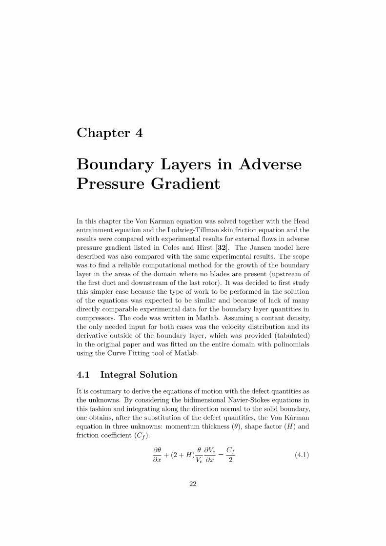
In this chapter the Von Karman equation was solved together with the Headentrainment equation and the Ludwieg-Tillman skin friction equation and theresults were compared with experimental results for external flows in adversepressure gradient listed in Coles and Hirst [32]. The Jansen model heredescribed was also compared with the same experimental results. The scopewas to find a reliable computational method for the growth of the boundarylayer in the areas of the domain where no blades are present (upstream ofthe first duct and downstream of the last rotor). It was decided to first studythis simpler case because the type of work to be performed in the solutionof the equations was expected to be similar and because of lack of manydirectly comparable experimental data for the boundary layer quantities incompressors. The code was written in Matlab. Assuming a contant density,the only needed input for both cases was the velocity distribution and itsderivative outside of the boundary layer, which was provided (tabulated)in the original paper and was fitted on the entire domain with polinomialsusing the Curve Fitting tool of Matlab.

4.1 Integral SolutionIt is costumary to derive the equations of motion with the defect quantities asthe unknowns. By considering the bidimensional Navier-Stokes equations inthis fashion and integrating along the direction normal to the solid boundary,one obtains, after the substitution of the defect quantities, the Von Kàrmanequation in three unknowns: momentum thickness (θ), shape factor (H) andfriction coefficient (Cf ).

∂θ

∂x+ (2 +H) θ

Ve

∂Ve∂x

= Cf2 (4.1)

22

Where the subscript e indicates the freeflow value. The goal was to solve theVon Kàrman equation for the momentum thickness, given a starting value.Since there are three unknowns, two more equations had to be added. Thechoice was for the Head entrainment equation [30] to evaluate the evolutionof the shape factor:

1Ve

d(HHθVe)dx = F (HH) (4.2)

where F (HH) is an empirical function and HH = δ−δ∗1

θ is linked to H [31]through:

F (HH) = 0.0306 (HH − 3)−0.653

HH = 1.535 (H − 0.7)−2.715 + 3.3and for the Ludwieg-Tillman skin friction equation:

Cf = 0.264 e−1.561H(ρeVeθ

µ

)−0.268(4.3)

With Cf the fraction coefficient and µ the dynamic viscosity. Given thestarting value from the experimental data of Hirst and Coles, the equationswere solved with a 4th order Runge Kutta integration scheme for space or witha simple forward Euler scheme. The experimental points were interpolatedon a number of auxiliary points. All computations had a ∆x given by theone percent of the domain. This solution will from now on named "integralsolution".

4.2 Jansen ModelAll results are also compared with the application of Jansen’s model, whichalso needs only the meridional velocity distribution as an input. The modelis suitable for the computation with or without blades and was tested also asan option for the non bladed domain. It was an early tentative to describethe growth of the boundary layer momentum thickness according to theequation developed from Schlichting [6] for external aerodynamics. It isdescribed in the paper of Jansen and it has been developed in 1967 [5]. It isone of the first attemps of computing the monodimensional boundary layerbased on flow conditions and it takes as unique input the meridional velocitydistribution along the compressor axis and its derivative. This is justifiedwith the consideration that the magnitude and rate of velocity decrease areby far the most important variables for the boundary layer development. Theidea is to find the axial variation of momentum thickness and of shape factorand from there find the displacement thickness directly used to computethe blockage. The integral formula from the momentum growth along theannulus is:

θ(X) = θ0 + 0.006

(∫ x=Xx=0 [Vm(X)]4 dx

)0.8

[Vm(X)]3.2

23

With Vm the meridional velocity θ0 some starting value function of theinlet conditions. Usually an initial displacement thickness is imposed at theinlet and θ0 is computed by assuming a reasonable shape factor (H = 1.4).Dussourd derives a simple empirical relation between the shape factor andthe momentum thickness [39], that can be used to compute the variation inH once θ(x) is known.

H(x) = 1.5 + 30∂θ∂x

(4.4)

In any case, this empirical formula is not always reliable and a simplerH = 1.4 is often imposed. Separation isn’t dealt with but a maximumvalus are imposed for H (H > 2.2 classically means separation). Theequations were discretised with a simple forward Euler scheme. The modelwas directly applied at the available experimental data (8-10 points) or on400 interpolated points along the domain. The scope of the interpolationwas to check whether the dependence on the ∆x was relevant or not. Inthese external flows Equation 4.4 was implemented.

4.3 Test 1: Flow 2200The Flow 2200 of Hirst and Coles is a boundary layer in mild positive pressuregradient, experimentally tested by Clauser [41]. The data for integralparameters are provided by Clauser, the Cf values and free stream velocityvalues are given in tabulated form. The freestream velocity profile is shown(Figure 4.1). Starting from the same initial values as the experimental datafor the displacement thickness and the momentum thickness, the equationsare implemented and the results for momentum thickness, displacementthickness and friction coefficient are given graphically (Figure 4.2 to Figure4.3). In this first test, the Jansen model performs better than the integralsolution. It is visible a certain influence of the interpolation on more controlpoints for the same model. Nevertheless, the trends are well followed in allcases. For the displacement thickness is shown a slight overprediction of theintegral solution and a slight underprediction of the Jansen model withoutinterpolated points. For the momentum thickness the latter solution alsoslightly overpredict the blockage. The interpolated Jansen is found to bethe model that best follows the evolution. For what concerns the frictioncoefficient, it is computed to be more or less half of the experimental valuefor all the domain, following the decrease of the latter.

24

Figure 4.1: Tabulated velocity and polynomial interpolation used (4th order).

Figure 4.2: Displacement thickness computed using Euler and Runge Kutta andJansen’s model on original and interpolated data compared with exper-imental data.

25

Figure 4.3: Momentum thickness computed using Euler and Runge Kutta andJansen’s model on original and interpolated data compared with exper-imental data.

Figure 4.4: Friction coefficient computed using Euler and Runge Kutta, comparedwith experimental data.

26


4.4 Test 2: Flow 2300The Flow 2300 of Hirst and Coles is a boundary layer in moderate positivepressure gradient, experimentally tested by Clauser [41]. The freestreamvelocity profile is shown (Figure 4.5).

In this second test, the integral solution performs better than the Jansenmodel. For the displacement thickness is shown a slight underprediction ofthe integral solution and a stronger underprediction of the Jansen model,whose computed values are approximately the half of the experimental allalong the domain. For the momentum thickness the underprediction ofJansen’s is enhanced, while the integral solution still performs quite well.For what concerns the friction coefficient, it is computed to be more or lessthe half of the experimental value for all the domain, following the decreaseof the latter.

27

Figure 4.6: Displacement thickness computed using Euler and Runge Kutta andJansen’s model on original and interpolated data compared with exper-imental data.

Figure 4.7: Momentum thickness computed using Euler and Runge Kutta andJansen’s model on original and interpolated data compared with exper-imental data.

28

Figure 4.8: Friction coefficient computed using Euler and Runge Kutta, comparedwith experimental data.

4.5 Test 3: Flow 4000The Flow 4000 of Hirst and Coles is a turbulent boundary layer in axiallysymmetric flow, with initial strong pressure rise followed by relaxation atconstant pressure. The experiment was performed by Moses [42], the tabu-lated data are provided by the same Moses. The freestream velocity profile isshown (Figure 4.9). In the third test, both models follow the trends quite well.While the integral solution slightly underpredicts the displacement thicknessat the end of the domain, the Jansen’s model resolves it more accurately andthe difference between interpolated and not interpolated evolution is apparentin the capacity of following the fast increase of displacement thickness. Theintegral solution resolves more precisely the peak of momentum thickness andslightly underpredicts it towards the end of the domain, while the Jansen’smodel fails the peak and slightly overpredicts the final value. No frictioncoefficient values were available for this case to compare.

29


Figure 4.10: Displacement thickness computed using Euler and Runge Kutta andJansen’s model on original and interpolated data compared withexperimental data.

30

Figure 4.11: Momentum thickness computed using Euler and Runge Kutta andJansen’s model on original and interpolated data compared withexperimental data.

4.6 DiscussionAs it is evident from the results, the solution is wrong for the frictioncoefficient, which is the half of the experimental value. The trends for thedisplacement thickness, nevertheless, are reasonably consistent with theavailable data for both methods. The integral solution overestimates it inthe Flow 2200 and underestimates it in the Flow 2300 and Flow 4000 butas an approximation and at least for the first part of the domain, it can beconsidered valid. Results between the Euler scheme and the Runge Kuttascheme showed differences only when the space step ∆x was large. TheJansen model can follow the trends less easily, failing in the Flow 2300, butit yields the best results for the Flow 2200 and acceptable values in the moresophisticated Flow 4000. The dependence on the ∆x is not generally seen tobe particularly relevant for the scope of the work. These results are usefulbecause both of these solutions will be explored in the program as a possibleoption for those parts of the domain without blades.

31

Chapter 5

Annulus Boundary LayerModels

The literature of annulus boundary layer models has been described inthe Chapter 2. In this chapter the general theory and ideas behind theimplemented models will be briefly explained, together with their intrinsiclimitations. The models that were used are the Jansen’s model (alreadydescribed in Chapter 4), the correlation of De Ruyck and Hirsch and themodified Aungier’s model. The first tests of implementation will then beexposed and the main criticities discussed.

5.1 Boundary Layer EquationsIn the case of bladed domain inside a turbomachine it was necessary toconsider a more complicated environment. The starting equations werethe three dimensional Navier Stokes equations, that again were reduced tobidimensional integral equations after the integration over the pitch and theboundary layer and the substitution of the defect quantities described in theIntroduction (Section 1.2). The unknowns are the same defect quantities,which are now projected in more directions. When considering the boundarylayer inside a compressor the viscosity terms and the blade force terms weretaken into account and the axisimmetric equations became, on the meridionalplane (m,n) (for derivation see [9]):

1r

∂rρWm

∂m+ ∂ρWn

∂n= 0

Wm∂Wm

∂m+Wn

∂Wm

∂n− sinφ

r(Wθ + ωr)2 = 1

ρ

[fm −

∂Pe∂m− ∂τm

∂n

]Wm

∂Wθ

∂m+Wn

∂Wθ

∂n− sinφ

rWm (Wθ + 2ωr) = 1

ρ

[fθ −

∂τn∂n

]

32

Where W is the relative velocity, φ the streamline curvature (or streamlineslope), τ the shear stresses on the wall, ω the blade angular velocity. Thesubscripts are the same described in the Introduction (Section 1.2): thesubscripts m stays for "meridional" and the subscript θ stays for "tangential".The subscripts 11, 12, and 22 indicate respectively the boundary quantityin the meridional direction, in a "mixed" direction (see definition, it con-siders velocities along m and along θ) and in the tangential direction. Theblade forces can be evaluated at the boundary layer edge where the outsideconditions are known and the shear stresses are identically zero.

fme = ρeWme∂Wme

∂m+ ∂Pe∂m− sinφ

rρe (Wθe + ωr)2

fθe = ρeWme∂Wθe

∂m+ sinφ

rρeWme (Wθe + 2ωr)

Exactly in the same manner as in the Von Kàrman equation, it is nowpossible to express the equations on terms of the defect quantities definedabove, obtaining the equations to be solved [9].

∂

∂m[rρeWme(δ − δ∗1)] = rρeWeF (5.1)

∂

∂m

[rρeW

2meθ11

]+δ∗1rρeWme

∂Wme

∂m−ρeWθe sinφ [Wθe(δ∗2 + θ22) + 2ωrδ∗2 ]

= r [τmw + fmeνm] (5.2)

∂

∂m

[r2ρeWmeWθeθ12

]+ rδ∗1ρeWme

[r∂Wθe

∂m+ sinφ(Wθe + 2rω)

]= r2 [τθw + fθeνθ] (5.3)

Where F is the symbol given for the empirical entrainment function(Equation 5.7).

5.2 De Ruyck’s and Hirsch’s CorrelationAfter Jansen’s model described in the previous Chapter (Section 4.2), thesecond model tested is a correlation set up by De Ruyck and Hirsch in theirpaper of 1981 [14]. The correlation is based on their model, often mentionedin literature as one of the most complete and reliable. In particular they startfrom the equations and they proceed with a derivation of all the unknownquantities, which they deduce from empirical observations and previous work.The model is composed with the Navier-Stokes equations integrate alongthe pitch and the boundary layer thickness. The complementary equations

33

that are used to close the model are the Head equation (4.2) and again theLudwieg-Tillman equation (4.3), with some changes to take into accountcompressibility effects. The formulation of suitable profiles for velocityand density has been detailed. Instead of using classical profiles for thetangential components of the velocity (for example a Mager profile), they tryto produce it dependent from the axial one, which is a usual power profile.A not negligible effort has been dedicated to the modelling and directioningof the force defects, whose importance is underlined: they represent allsecondary flow effects, they allow for the quasi-equilibrium situation foundin compressor after some stages, they heavily influence efficiency directly(tangential forces affect torque) and indirectly (axial forces contribute todisplacement thickness). The relevant terms are recognised to be caused byblade loading variation, secondary stresses due to non-axysimmetry of theflow, variation of pressure gradient and blade shear stress. The defect forceswere estimated using correlations that take into account all of these effectsand accurate local flow analysis were performed in order to establish themagnitude of these forces in the meridional and tangential direction. Finallya correlation is proposed which is supposed to give a fast but neverthelessreliable estimation of the relevant boundary layer quantities, based on anumber of geometrical data and flow properties along the domain. Startingfrom the usual equations a growth for the momentum thickness is derivedwhich has the following form:

(∆θ11)stage = p− qθ11 (5.4)

where p and q are:

p =∑R,S

c cos γ2 cos2 α

[Cf

(1 + ψ

c

)cosα∞ + ΛC2

Lσ

]

q = 2(2 +H)AV R− 1AV R+ 1 + sin 2|α∞|

2 kf1− e−kσ

ψ

Where all the data are: α∞ = αin+αout2 , with α the absolute flow angle

with respect to the axial direction, ψ the mass flow coefficient (ratio ofaxial velocity over rotational velocity), CL the lift coefficient, AV R the axialvelocity ratio (ratio of inlet axial velocity over outlet axial velocity), σ thesolidity, λ = K tc

s + L2 , with tc the tip clearance, K and L empirical constants

and c the chord. Then the concept of equilibrium of the boundary layer isemployed: at some point along the compressor an equilibrated thickness ofthe boundary layer (and of the boundary layer quantities) will be established.This represents the fundamental hypothesis in the procedure. With thishypothesis, one has that at some point the ratio between p and q will stabiliseand:

θeq11 = p

q

34

If this is true, then equation (5.4) can be rewritten

∆(θ11 − θeq11)θ11 − θeq11

= −q

which is the discretisation of

θ11 − θeq11 = (θ11 − θeq11)in e−∑

stagesq (5.5)

If one considers some initial q0 then

e−q0 = 1− θin11θeq11

and equation (5.5) becomes:

θ11 = θeq11

[1− e−(q0+

∑stages

q)]

(5.6)

Once the momentum thickness is known, one can assume some reasonableshape factor and obtain in the same way the displacement thickness andfinally the blockage. Given the well structured environment in which themodel was operated, another step was performed to obtain the final operatingmodel. In particular, the approximate integral solution method tested for aturbulent boundary layer in adverse pressure gradient in Chapter 4 (describedin Section 4.1) was implemented as an option together with the Jansen modeldescribed in the same Chapter 4 (Section 4.2) to cover the parts of thedomain where no blades are present. This means the beginning and the endof the domain, where dummy ducts are present. This choice was justified bythe fact that it was reckoned that in those areas the flow would behave in arelatively well behaved manner.

5.3 Modified Aungier’s ModelAfter having explored the simple model from general external aerodynamicsand a more specific correlation procedure which takes into account a largequantity of compressor data, it was decided to try to consider the directsolution of the equations using an approach similar to the one described inthree dimensions in Aungier’s book [9] but in two dimensions, also employedfor a number of cases in a recent paper from Banjac, Petrovic andWiedermann[40]. Starting from the same theoretical background of De Ruyck and Hirsch,Aungier proposed a direct application of the solutions in which the velocityprofiles of the boundary layer will update depending on the freeflow conditionsand converge to a stable solution for each meridional station. The equationsemployed to close the problem are again the Ludwieg-Tillman equation(4.3), used with values from the freestream direction, but instead of using

35

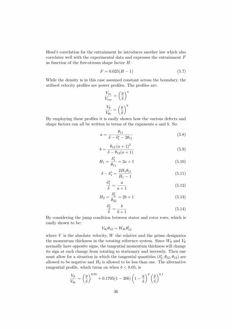
Head’s correlation for the entrainment he introduces another law which alsocorrelates well with the experimental data and expresses the entrainment Fas function of the free-stream shape factor H:

F = 0.025(H − 1) (5.7)

While the density is in this case assumed constant across the boundary, theutilised velocity profiles are power profiles. The profiles are:

VmVme

=(y

δ

)aVθVθe

=(y

δ

)bBy employing these profiles it is easily shown how the various defects andshape factors can all be written in terms of the exponents a and b. So:

a = θ11δ − δ∗1 − 2θ11

(5.8)

b = θ12 (a+ 1)2

δ − θ12(a+ 1) (5.9)

H1 = δ∗1θ11

= 2a+ 1 (5.10)

δ − δ∗1 = 2H1θ11H1 − 1 (5.11)

δ∗1δ

= a

a+ 1 (5.12)

H2 = δ∗2θ22

= 2b+ 1 (5.13)

δ∗2δ

= b

b+ 1 (5.14)

By considering the jump condition between stator and rotor rows, which iseasily shown to be:

Vθeθ12 = Wθeθ′12

where V is the absolute velocity, W the relative and the prime designatesthe momentum thickness in the rotating reference system. Since Wθ and Vθnormally have opposite signs, the tangential momentum thickness will changeits sign at each change from rotating to stationary and inversely. Then onemust allow for a situation in which the tangential quantities (δ∗2 , θ22, θ12) areallowed to be negative and H2 is allowed to be less than one. The alternativetangential profile, which turns on when b < 0.05, is

VθVθe

=(y

δ

)0.05+ 0.1705(1− 20b)

(1− y

δ

)2 (yδ

)0.1

36

As already mentioned, the correlation for the experimental data on forcedefect of of Koch and Smith was found to be more satisfying by the sameAungier with a differend normalisation of both the defect and the displacementthickness. The equation proposed for both the defects (νm ≈ νθ followingthe hypothesis of Mellor and Wood [10] of blade force in the same directionas the freestream blade force) is:

ν0 = (0.12g + t/2) (8θ11/g)3

1 + (8θ11/g) (5.15)

where accordingly to [40] the average of the momentum thickness originallypresent was substituted with the local momentum thickness, t is the bladeclearance and g the staggered spacing. The solution procedure proposedby Aungier is iterative for each meridional station and it lets the boundaryproperties vary to accomodate the changes in external flow. In particularone defines first inlet values such as H = 1.4 and m = 1/7 (7th power law).The boundary layer is constrained to be turbulent by imposing a minimumReynolds number based on θ11 (Reθ ≥ 250). The iterative process is:

• Estimate θ11 and θ12 from the simplified Equations (5.2) and (5.3)using the inlet values at the previous station and keep H1 and H2constant.

∂

∂m

[rρeV

2meθ11

]= 0

∂

∂m

[r2ρeVmeVθeθ12

]= 0

• (*) Compute all necessary boundary layer quantities from Equations(5.8) to (5.14)

• Compute entrainment, wall shear stresses and blade force defects

• solve the complete Equations (5.1), (5.2) and (5.3) for (δ− δ∗1), θ11 andθ12

• Compute all necessary boundary layer quantities from Equations (5.8)to (5.14)

• Check for convergence on θ11, H1, ν

• Back to (*) if not converged, next meridional station if converged.

Once all the boundary layers defects are known, it is possible to computethe blockage. The two dimensional version of this approach was preferredbecause according to [40] it still gives very good results for quite general casesand the quantity of empirism is reduced with respect to the complete version.The assumptions are the same of the general model. The employed equation

37

was only Equation (5.2), which was simplified (the tangential terms did notplay a role anymore). Together with Aungier’s correlation for entrainment(Equation (5.7)) the usual Ludwieg-Tillman closed the problem. The iterationprocedure remained the same. The approach taken for the areas withoutblades was the same described for the previous model (at the end of Section5.2).

5.4 BlockageThe blockage can be defined in different ways, the blockage implementedin the model is the effective area found from the effective radius given bythe nominal radius minus the displacement thicknesses at hub and and plusthe latter at tip over the nominal area. It is an useful indication of howmuch is the deficit of area in percentage of nominal area due to the presenceof the boundary layer. In the code it is divided in an "inlet" and "outlet"contributions, defined in the same way. The δ∗ in the formula is the axial(δ∗ ≡ δ∗11), kB is the blockage, or blockage factor.

kBhub = (Rhub + δ∗hub)2 −R2

hub

R2tip −R2

hub

· 100 (5.16)

kBtip =R2tip − (Rtip − δ∗tip)2

R2tip −R2

hub

· 100 (5.17)

5.5 Critics to the modelsAfter the detailed analysis of the flow features (based on available data) themost likely conclusion was that none of the above described models wouldprovide precise solutions. The dependencies and interdependecies of the flowproperties are hard to predict and generalise and the real behaviour of theflow too complex.

In particular, Jansen model tries to estimate the growth based only onthe velocity distribution, completely neglecting all detailed flow featureswhich nevertheless proved to be fundamental (to mention some, neither tipclearance nor force defects are taken in consideration). The correlation isbuild upon more precise models and performed well in the cases where itwas tested. It considers all geometric features and a large number of flowproperties to deliver its results. Anyway, its greatest defect is that it is builtupon the basic assumption of the reaching of an equilibrium state, whichtheoretically is reached after a number of stages and therefore may simplynot be usable for low pressure compressors. The last model was the mostcomplex but most promising. It solves the equations of the boundary layer byassuming the velocity fields within the layer and iterating until a stable point

38

is reached, considering flow properties, geometrical details and empiricalcorrelations for the force defects. Nevertheless, it was also build and testedfor some particular cases and its performances for more general cases arehard to predict.

In any case, computational results are available for all of these models thatshow good performances despite all apparent difficulties. What was reckonedwas that the models were likely to perform quite well when tested in theprecise environment where they are developed for. Anyway and to conclude,for the type of work to be performed in this case extreme precision was notseeked and a reliable estimate of the displacement thickness evolution alongthe domain in the compressor cycles was believed possible to be achieved.

5.6 ImplementationFor practical reasons, all tests were first conducted on a particular environ-ment: the NASA TP 1493 at 50 percent of the design speed. The completedescription of the fan is to be found in the next Chapter 6. At the momentof the beginning of the work the blockage was not taken into considerationif not in the initialisation value at the first timestep, after which the firstand last streamlines in the radial direction were simply not moved anymore.The way in which the model was introduced in the software was throughthe update of the radial domain. In particular at each iteration now thecurrent blockage will be taken into account and the first and last streamlineswill be updated correspondely starting from the physical domain and simplyadding the displacement thickness computed at that meridional station. Themodels tested in this case were: Jansen model on all the domain (1), Aungiermodel in bladed domain with the integral solution where no blades arepresent (2), correlation in bladed domain with the integral solution where noblades are present (3), Aungier in bladed domain with Jansen upstream andintegral solution downstream where no blades are present (4) and correlationin bladed domain with Jansen upstream and integral solution downstreamwhere no blades are present (5).

Due to the high sensitivity of the software on the boundary conditions,to the fact that the calculated value from some of the models was oftensensibibly different and surely to the doubtful operating conditions where thetest were conducted, the first results from the models were not incouraging.In particular, when first testing the correlation, the Jansen solution andthe 2D Aungier model the only model converging over the whole range ofmassflows (12 massflows were first considered for the operating conditionsat 50 of speed, ranging from 13.05 kg/s to 18.55 kg/s) was the latter, whilethe correlation did not converge if not for the first mass flow and the Jansensolution crashed in the moment of the first use of the computed values.

The models were inserted with some modifications.

39

First, the models were not always yielding physically acceptable results.This is because in the cycle of iterations it is possible, particularly at thebeginning or at mass flow variation, that some odd values would arise. Toprevent these potentially instable situations some control switch were insertedin the models. Particularly, in the correlation a switch would check whetherthe computed equilibrium solution would be physically acceptable or not andin case of negative results it would just switch to the previously computedsolution. In the Jansen model the computation for H was taken away and thelatter was simply put equally constant to 1.4 and a check on the maximumpossible area blockage was imposed at 25% of the nominal area for both huband and tip (as suggested in the original paper [5]). In the Aungier’s model,the meridional H was also limited to be less than 2.2 and the boundary layerwas limited to be turbulent with a check on the Reynolds number basedon momentum thickness (Reθ > 250) and the same switch was employedto go back to the previous value in the occurrance of odd values. Finally,for what concerns the integral solution, it needed an input value differentfrom zero for the initial displacement thickness because of the computationof the friction coefficient. The minimum accepted value for the displacementthickness was 0.001 m and therefore this was the imposed initial value at thebeginning of the domain. In general if no integral solution is implementedthe starting value is kept to zero for the displacement thickness.

Second, the immediate crash of the computation was probably underlyingan issue about the flexibility of the streamlines generated by the main code(with flexibility is here meant their ability to be displaced from one iterationto the next without compromising the calculation itself). The inserted modelswould fit a well structured environment and not all the consequences of theupdate of the streamline were clear from the beginning. This highlighted thenecessity of some sort of numerical damping. There is a factor imposed bythe user that controls the damping of the streamlines but that paramenter isnot found to be a relevant for what concerns the launch of the calculation. Ithas instead a relevant effect on the duration of the latter, which is increasedin a significative manner. An analysis was performed for trying to detect thesource of failure for the Jansen model, that would make the computation crashas soon as it was activated. The possible sources of mistake and numericalinstability are recognised to be the first displacement when the model isactivated and the streamlines pass from the initialised to the computed value,the large value of the displacement itself or the calculated distribution.

In the Figure 5.1 is represented the table with the maximum computedabsolute blockage in the domain for the inlet and outlet of the blade rowsand with the maximum computed variation from the initial values for allthe models tested. These data were gathered at the precise moment whenthe models were activated. As it is apparent, the immediate crash of thecomputation is likely to be due to either the large computed value itself orto the large change in the first implementation. Anyway, when scaling the

40

Figure 5.1: Comparison table for the maximum value of the norm of the computeddisplacement thickness and the delta between the initialised value andthe computed value at inlet and outlet and at hub and tip of all tur-bocomponents. Each column is relative to a model, in order: Jansen,Aungier with integral solution, Correlation, Aungier with Jansen, Cor-relation with Jansen. The highlighted column (Jansen model) clearlyshows the largest value in both absolute value and delta. The 1* columsindicates the results from the Jansen model scaled by a factor 0.5.The "result" row indicates whether the code accepted or not the firstintroduction of the computed value and not whether the code convergedor not. To note the first application of the security switch at the tipfor the cases with correlation: the delta with respect to initialisation iszero because the former value was kept.

displacement thickness obtained from the calculation of a factor 0.5 (seecolumn 1*), both the absolute value and the variation from the initial valuetake more common values but still the computation doesn’t start.

The conclusion of this work of analysis is that neither the jump conditionnor the magnitude, recognised as possible sources, are the main actor inthe failure. Most likely, the computed distribution of the boundary valuesis not correct and this leads to some back error and to the failure of thecalculation (which always happens at the level of the computation of theupdated computational grid).

The next chapters will see the description of the application of the modelsin these latter case and in more operating condition. The models whichyielded the best results in the previous analysis will be studied. Even ifthe direct implementation of some of the not ideal models will result ina failure of the computation, the model evolution will still be performedin background and the result analysed. With "background" is here meantthat the model will calculate the boundary layer quantities along all thecomputation, but its results won’t be used for the next iteration; instead the

41

input values imposed by the user will be kept thoughout all the computation.

42

Chapter 6

Test on Available Geometries

Current geometries implemented on the software at the time of the beginningof the work included different one to two stages models for transonic fanssuch as the NASA TP 1493. The selected geometries were the NASA TP1493 and its first rotor operating alone, the designed NASA Rotor 67. Thesegeometries aren’t in fact ideal for the models for they are of limited lengthand the boundary layer will not have the possibility to develop in a ordinatemanner. Anyway the scope of the work was to look at a general-as-possiblemodel and it was interesting too see how they would perform. In this chapterare described the steps followed and the results obtained. The numericalresults will be compared with the experimental results for what concernsoverall compressor performances and for the case of the complete fan alsodirect data for the boundary layer quantities are available and discussed.

6.1 DescriptionThe NASA TP 1493 is a two stage transonic fan which was derived from aprevius design [52] by reducing the aspect ratio of the blading and conse-quently the need for midspan dampers. It was presented in 1979 from Uraseket al. in a report where all geometrical data and design performances werelisted [42]. Low aspect ratio turbomachinery blading has the advantage ofhaving fewer blades and lower production costs. Moreover, the aerodynamicloss associated with dampers is relevant and often precludes the achievementof high efficiencies. In particular, tests for the first design of the two stagesfan yielded an overall efficiency approximately 5 percentage points less thanits design value, while with the new low-aspect-ratio blading the efficiencywas two percentage points more than the design value. The fan was designedfor a weight flow of 33.248 kg/s with a 100% design velocity of 16042.8 rpm.In the single rotor configuration the designed pressure ratio is 1.63 at thesame mass flow and design velocity as the complete fan. The diagram ofthe complete compressor and of the single rotor will be shown in the results

43

Figure 6.1: The Rotor 67. [53]

Figure 6.2: The flowpath of the TP 1493 with the position of the 3 measuringstation. The higher-aspect-ratio rotor of the previous design is alsosketched. [42]

section.The fan NASA TP 1493 has no inlet guide vane or exit guide vane. In

the first stage rotor, the blading was of MCA (Multiple Circular Arc) crosssection across the entire blade span; in the second stage rotor the blading wasMCA from the tip to 44 percent of span and DCA (Double Circular Arc) overthe remainder. Both stators had DCA blading. The maximum thickness forthe MCA was specified at 50% of the span and the transition point locatedwhere a normal passage shock was predicted. A summary of the blade datafor rotors and stators is given in the reference [42]. Graphical representationof both geometries is given in Figure 6.1 and Figure 6.2 respectively for therotor alone and for the complete fan.

44

6.2 ExperimentsThe fan was tested at the Lewis multistage compressor facility over a range ofmass flows at different speeds. The experiments yielded overall performancedata at 50%, 70%, 80%, 90% and 100% of design speed. Standard atmosphericconditions of temperature and pressure were used. The experimental set uphad three measuring stations along the domain measuring temperatures andpressures. The stations are positioned at the fan inlet and behind the twostator-blade rows, as visible in Figure 6.2. Total pressure, total temperatureand flow angle were measured with a combination probe. Two combinationprobes were used at Station 1 and Station 2, while 4 combination probeswere positioned after the second stator (Station 3). The data downstreamthe single blade elements were extrapolated along design streamlines startingfrom the data registered at the measuring stations. The rotor 67 in a onlyrotor configuration was also extensively tested by Strazisar et al. in 1989through anemometry [53].

6.3 ModellingBoth the two stages fan and the configuration with the single rotor weremodelled with 31 streamlines and 13 geometrical reference points. Thegeometrical data for the radial and axial position of the blades and for theflowpath were available from the original reports [42]. 42 points were usedfor both the tip and the hub flowpaths. Three dummy ducts were insertedupstream of the first rotor and other three ducts were positioned downstreamof the last stator (or downstream of the single rotor), to increase the stabilityof the flowfield computation. The flowpath distribution for these additionswas represented by straight extensions of the flowpath when needed. InFigure 6.4b is possible to see the overall grid. The imposed working fluidwas air, the average inlet temperature 288.15 K and the average inlet totalpressure 101325 Pa. Slight distortion of the inlet flow field was imposed.

45

(a) Geometry. (b) Grid solution.

Figure 6.3: The geometry and grid solution for the NASA Rotor 67 in single rotorconfiguration.

46


Figure 6.4: The geometry and grid solution for the NASA TP 1493.47

6.4 Comparison with Experimental Boundary Quan-tities

First of all a comparison with the available experimental data was carriedout, to verify whether the models were yielding reasonable results. Theexperimental data came from the work of Ball et al. in 1983 [47]. Theobjective of that study was to obtain detailed flow measurements in the casingboundary layer of a two stage fan in order to expand the limited experimentaldata base available from high speed, high pressure ratio multistage fan andcompressors for use in modelling and code verification. The fan had beendesigned taking into account blockage allowances of 0.013 cm at the firststage rotor exit, 0.018 cm at the first stage stator inlet and 0.020 cm at allothers leading- and trailing edge locations. These values were the same forhub and tip.

The data for the boundary layer surveys had been taken at three massflows ranging from maximum flow to near stall at design rotative speed (34.01kg/s to 34.63 kg/s at 16042.8 rpm).

The two stage fan was tested in the NASA Lewis multistage compressorfacility. 10 radial surveys of the flow conditions between 1 and 30 percentof passage height were taken at 5 axial stations: at fan inlet and behindeach blade row (see Figure 6.5). Total and static pressure, total temperatureand flow angle were recorded at each station. Wall static pressure wasalso measured at each station. All pressures were measured with calibratedtransducers. Two combination probes were used at station 1 to 4 whiledownstream of the last stator were used four combination probes. Theprocedure used in calculating the end-wall boundary layer parameters frommeasured stations was based on the matched asymptotic expansion extendedto turbomachinery flow by Mellor and Wood [10].

Figure 6.5: The flowpath of the TP 1493 with the position of the 5 measuringstation. [47]

48

In this first analysis computed results for the 50 percent of speed havebeen compared with the 100 percent of speed of the experimental case. Thisis because the goal was to see whether the main trends were respected andbecause the 100 percent of speed was reached just with one of the models.δ on the ordinate axis represents in all the following pictures (Figure 6.6to Figure 6.10) the axial displacement thickness elsewhere indicated withδ∗11. In these plots, the legend indicates the model in use, the percentage ofrotational speed and the massflow at which the boundary layer was computed.The model denomined "Aungier" stays for the Aungier model with integralsolution in the domain without blades, the model denominated "Jan + Aung"stays for the model with Jansen’s model upstream of the bladed domain andintegral solution downstream, the models denominated "Jansen" and "Corr"stay respectively for Jansen’s model and the correlation.

In figures (Figure 6.6 and Figure 6.7) it is shown the performance ofthe first running models for the 50 percent of speed compared with theexperiental results at 100 percent. Since the experimental data were availableat three different mass flows, also the computed values have been shown atthree different mass flows: near stall, near peak efficiency and near choke.

In the next two pictures instead (Figure 6.8 and Figure 6.9) the result ofthe other two models running in background are shown for the same velocity.The Jansen’s model was clearly failing in the computation of the sixth axialposition at a mass flow of 13.15 kg/s and therefore the plot presents theresult for a mass flow of 13.55 kg/s, always at 50 percent of speed.

49

Figure 6.6: The experimental data from [47] compared with the results at 50percent of speed of the Aungier model with integral solution in thedomain without blades.

Figure 6.7: The experimental data from [47] compared with the results at 50percent of speed of the Aungier model with Jansen model upstreamand integral solution downstream the bladed domain. [47]

50

Figure 6.8: The experimental data from [47] compared with the results at 50percent of speed of the Jansen’s model, run in background.

Figure 6.9: The experimental data from [47] compared with the results at 50percent of speed of the correlation with integral solution in the domainwithout blades, run in background. [47]

51

The conclusions relative to this preliminary comparison are following.Two main observation were drawn from this analysis. The first observation isthat the trends for the evolution of the boundary layer are well represented.There are not many informations in literature about the behaviour of thecompressor boundary layer at partial speed, but it seems reasonable thatthe boundary layer will be smaller at reduced rotational speed and that thepeaks due to the effect of rotors and stators will be less sharp. Furthermore,the expected decrease in boundary layer thickness visible in the experimentalcase is also found in the computational result.

Nevertheless, the trends for the higher mass flow are wrong accordinglyto the experimental data. As seen in the experiments and in the work ofHirsch and Denton mentioned in Chapter 2 [46], the higher mass flow aswell as the near to stall condition would both cause a thicker displacementthickness.

Since the experimental data suggest that the trend for higher mass flowshould be the opposite, it might be the case of a wrong evolution of theboundary layer in the first part of the domain, without blades, which mightnot take into account in a proper way the variation of the mass flow andtherefore yield wrong starting values for the displacement thickness. As itcan be seen from a comparison between Figure 6.6 and Figure 6.7 the startingpoint has a strong influence on the later development (the only differencebetween the two models is the treatment for the first part of the domain).A more suitable way to compute the boundary layer thickness that wouldpossibly yield a more reliable starting point is therefore here presented. InAungier [9] the suggested starting displacement thickness takes into accountthe massflow and it is described by:

2πrρeVmeδ∗1 = 12Bm (6.1)

Where r is the radius, Vme the meridional velocity outside of the boundary, δ∗1the axial displacement thickness, m the mass low and B a blockage value atinlet, which is defined from Aungier starting from the displacement thicknessbut is suggested to be B = 0.02 for both hub and tip. This solution wasimplemented imposing a simple linear growth of the boundary layer, thatwould reach the requested starting point computed with Equation 6.1 at thebeginning of the bladed domain. The simple growing line has been the bestoutcome in a number of possible profile tested for the inlet ducts, amongwhich also the Blasius solution for laminar flow was tested, but did notconverge. The quasi-linear evolution proved to be the most effective strategyand it yielded convergence on almost all the compressor operational range.In Figure 6.10 are shown the results for 50 percent and for 100 percent ofthe speed. The label for this case is "Direct". While at 50 percent of speedthe same mistake is still generated as before (lower displacement thicknessgrowth at higher mass flow), at higher speed the trend for the mass flow

52

Figure 6.10: The experimental data from [47] compared with the results at 50percent of speed and at 100 of speed of the Aungier model with alinear growth upstream and the integral solution downstream of thebladed domain.

variation seems to be improved: at 100 percent the trend inverts and thehigher mass flow boundary is correctly computed to be higher than the peakefficiency. The stall condition, regrettibly, could not be computed at thisrotational velocity.

In any case, the trend of the boundary layer at 100% of velocity appearsto be inverted with respect to experimental data (the layer grows throughoutthe fan). This might be due to the fact that the starting value of displacementis still different from the one in the experimental case. As seen in Cumpsty,the thickness of the boundary layer itself with respect to the tip clearance is arelevant parameter that might affect the usual trends [35]. Another possibleexplanation of this behaviour is that there could exist a "natural" boundarylayer exit condition dependent on the blading and the flow conditions thatwould modify the usual trends depending on the entrance condition, assuggested by the same Cumpsty [34].

To conclude, with the last model the trends for the dependence of theboundary layer on rotational velocity and mass flow variation seem onlypartially found. The trend for the higher mass flow at 50 percent of thespeed is apparently wrong, but it is only compared with informations at 100percent of speed. The same model that at 100 percent of speed predicts acorrect trend for higher mass flow predicts at 50 percent the same "wrong"trend. This might suggest that this dependence is in fact inverted at lowvelocity. No experimental data at partial speed is available to confirm ornegate this assertion.

However, the disagreements don’t seem to be inacceptably important andas anticipated, the model covers almost all the compressor map for this case.

53

Figure 6.11: Compressor map of the NASA Rotor 67 in single rotor configurationcompared with experimental results, the boundary layer is initialisedand kept constant. The computed lines are coloured.

6.5 ResultsThe first step in the evaluation of the models is a tentative to run thegeometries with already established conditions. The results on the compressormap are very good when compared with experiments (see Figure 6.11 andFigure 6.12). With the imposed boundaries (total pressure, total temperature,flow angle at inlet and fixed boundary layer blockage) most of the points onthe map could be completed. The failure in the convergence of some of thepoints is due to the fact that the flow angle distorsion at inlet is imposedduring these tests. The blockage factors were tuned to obtain the best matchwith numerical results.

Starting from these reference values, the curves computed with the modelsare shown for both the rotor in single configuration and the complete fan,for the cases in which the computation converged. First for the rotor (fromFigure 6.13 to Figure 6.17) and then for the complete fan (from Figure6.18 to Figure 6.20). In these plots, the legend indicates the model in use.The model denomined "Aungier" stays for the Aungier model with integralsolution in the domain without blades, the model denominated "Direct" isthe model with a quasi-linear distribution in upstream of the the bladeddomain and integral solution downstream, the model denominated "AungierJansen and Int Sol" stays for the model with Jansen’s model upstream ofthe bladed domain and integral solution downstream.

54

Figure 6.12: Compressor map of the NASA TP 1493 with experimental results, theboundary layer is initialised and kept constant. The computed linesare coloured.

Figure 6.13: The computed map for 50 percent of speed for the single rotor: thecase with no boundary layer model inserted is compared with theconverged solutions with the model.

55



56



57

Figure 6.18: The computed map for 50 percent of speed for the complete fan: thecase with no boundary layer model inserted is compared with theconverged solutions with the model.

Figure 6.19: The computed map for 70 percent of speed for the complete fan: thecase with no boundary layer model inserted is compared with theconverged solutions with the model.

58

(a) Displacement thickness. (b) Tangential force defect.

Figure 6.20: Defects over pressure rise ratio. [34]

6.6 DiscussionEven if the computed values for the boundary layer thickness are sensiblydifferent from the ones implemented in the code without model, which weresimply imposed to be growing along the compressor axis and of a similarmagnitude, the compressor map for the simple Rotor 67 could be completedfor both models: the Aungier with integral solution and the Aungier withlinear distribution upstream and integral solution downstream the bladeddomain. The results are well fitting the experiental performance curves andare only slightly different from the case without model. Instead, the fanperformance map couldn’t be completed: the Aungier with integral solutioncould only converge up to the 70 percent of velocity, while the Aungier withlinear distribution upstream and integral solution downstream the bladeddomain could only not converge at 80 percent of the speed. The compressormaps for the two models for the rotor and for the fan for just the one thatconverged most follow in Figure 6.21, Figure 6.22 and Figure6.23.

To conclude, the Jansen model and the correlation didn’t yield any usefulresult as expected. The modified Aungier model was able to follow at leastthe main trends of the unusual development of the boundary layer in atransonic two stage fan, when it was initialised in the proper way. Theimposed inlet condition was seen to have an important effect and to bedeterminant in the convergence or not of the model. The through-flow codeanswered positively to the additional model.

59

Figure 6.21: Compressor map of the NASA Rotor 67 in single rotor configurationcompared with experimental results, the boundary layer is computedby the Aungier’s model with integral solution in the not bladed domain.

Figure 6.22: Compressor map of the NASA Rotor 67 in single rotor configurationcompared with experimental results, the boundary layer is computedby the Aungier’s model with linear distribution upstream and integralsolution downstream the bladed domain.

60

Figure 6.23: Compressor map of the NASA TP 1493 compared with experimentalresults, the boundary layer is computed by the Aungier’s model withlinear distribution upstream and integral solution downstream thebladed domain.

61

Chapter 7

Test on Multistage Geometry

For the test in a multistage environment, a number of different designswere taken in consideration. In particular all publicly available data for theNACA transonic 3-stage [48], a NASA design for a 5 stages tested only ona preliminary 3 stages design [49], the BBC transonic 4-stage described inthe AGARD 175 [46], the NACA transonic 5-stage [3] , the NACA 8-stage[2], the NACA 10-stage [50] and a GE 10-stage [51] were analysed and itwas concluded that the only geometries for which all necessary data wereavailable were the NASA 3-stage and the transonic NACA 5-stage. Sincethe goal of the test was to study the performances of the models on alarger domain, the final choice has been for the 5 stage. It is the largestgeometry ever tested on the code, which nevertheless is extensively validatedon high-speed compressors. In this case the model is supposed to give morereliable results with respect to the application on fans. The numerical resultswill be validated by comparison with the overall experimental compressorperformances, since no direct boundary layer data are available. In thischapter the steps followed and the results obtained are described.

7.1 DescriptionThe NACA 5-stage axial compressor operates with relative transonic relativeinlet Mach numbers for all rotor blade rows. It was designed in 1954 tostudy the problems arising from the compounding of transonic stages [3].By increasing the inlet relative Mach number the stage pressure rise can beincreased and the same desired pressure ratio is obtained with a fewer numberof stages. This reduces the compressor size and weight. The compressoris designed to produce an overall total pressure ratio of 5.0 at a rotor tipspeed of 335.3 m/s. The casing of the compressor has a constant diameter of0.508 m and the hub-tip ratio at the inlet of the first rotor is 0.5. A speedof 12605 rpm was calculated from this data, which will henceforth be thereference for the 100% of the rotational speed. The design mass flow was

62

Figure 7.1: Geometry of the NACA 5-stage.

30.617 kg/s. The NACA 5-stage has not Inlet Guide Vane (IGV) or ExitGuide Vane (EGV). All rotor blades are DCA (Double Circular Arc), whilefor the stators the first two rows are DCA and the last three rows have aNACA65 thickness distribution on a circular arc meanline. A summary ofall geometrical data can be found in [3].

7.2 ExperimentsThe compressor was tested over a range of mass flows at different speeds.The tests delivered overall performance data as well as individual blade rowdata. The overall performance was tested from the 40% to the 100% of thedesign speed, while individual blade rows experiments were conducted from70% to 100%. The pressure and temperature conditions during the test werethe NACA standard sea level, i.e. respectively 101314.1 Pa and 288.17 K.

Measuring stations were positioned all along the compressor measuringtemperatures and pressures. The numbered stations are visible from theFigure 7.1. The engine inlet bellmouth (station 0) measures the inlet stag-nation conditions. Measuring stations 1 and 2 were upstream of the firstrotor, respectively 26.7 cm and 10.1 cm from the inlet rotor leading edgeat hub. Stations 3 to 12 were positioned behind each following blade rowand the final measuring point (station 13) was 50.8 downstream of the fifthstator trailing edge. The instrumentation was placed approximately 22.9 cmbehind each rotor blade row and 7.62 cm behind each stator blade row.

63

To study the performance of individual stages, three series of testescovering a range of flow rates were run, during which groups of blade rowswere instrumented successively (respectively first two stages, stage three andfour, stage five). Each serie covered the operative range of the compressorfor speeds from 70 to 100 percent of design speed. Radial distributions ofstatic and total pressure, total temperature and flow angle were obtainedthrough the use of two combination probes and static pressure probe behindeach rotor and a wake rake and static pressure probe behind each stator. Alldata are available in [52] and [53].

7.3 ModellingThe code had to be slightly modified to make the geometry run. In particularit was failing in the calculation of the design incidence speed (probably dueto the guesses for the secant interpolation method used) and the latter wastherefore inserted manually in the corrispondent subroutine. The 5-stagecompressor was modelled with 31 streamlines and 13 geometrical referencepoints. The geometrical data for the radial and axial position of the bladesand for the flowpath were not available from the reports and were thereforeextracted from the same picture show above (Figure 7.1). The tip clearancewas 1% of the annular spacing. 22 points were used for the tip flowpath and98 points for the hub flowpath. Three dummy ducts were inserted upstreamof the first rotor and other three ducts were positioned downstream of the laststator, to increase the stability of the flowfield computation. The flowpathdistribution for these additions was represented by straight extensions of theflowpath when needed. In Figure 7.2b is possible to see the overall grid. Theimposed working fluid was air, the inlet temperature 288.15 K and the inlettotal pressure 101325 Pa. No distortion of the inlet flow field was imposed.

64


Figure 7.2: The geometry and grid solution for the NACA 5-stage.

65

Figure 7.3: Converged operating points compared to the experimental compressormap of the NACA 5-stage.

7.4 ResultsThe comparison of results is in this case more limited. Due to time constraints,proper initialisation blockage factors used in the case without model insertedcould be found only at the particular operating conditions of 14 kg/s ofmass flow and at a rotational speed of 6600 rpm (approximately 52% ofthe speed). From this determined condition, thanks to the structure of thesoftware, almost all compressor map could be completed (at least partially).At every timestep imposed mass flow and rotational speed were changed atsmall steps until the desired compressor curve could be drawn. Figure 7.3shows the comparison of the converged points on the compressor diagramwith experimental results.

The results match pretty well with the experimental data in the consideredoperating conditions. It is reckoned that the reason why the computationcan not converge to near stall operation is that the "boundary layer", whichis not computed yet but it’s taken into account as if it was constant bykeeping the first and last streamline in the same position, is acceptable fora low mass flow and low rotational speed but it is not thick enough to berealistic in the near stall region. Due to the fact that all the compressor mapis built upon one converged initialised operating condition it was supposedto be likely that the convergence would just be met in particular conditions.Nevertheless, this would be enough to test the results from the models and infact, it was expected that the model themselves, since they used a computedboundary layer thickness, would converge more in the map. This was not thecase. In Figure 7.4, Figure 7.5 and Figure 7.6 the converged operating pointsare shown compared with the case without the models. The models that

66

Figure 7.4: The computed map for 50 percent of speed for the NACA 5-stage:the case with no boundary layer model inserted is compared with theconverged solutions with the model.


could converge are the same as in the previous case: "Aungier" is the namethat indicates the Aungier’s model with integral solution in the not bladeddesign and "Direct" indicates the Aungier’s model with linear distributionupstream and integral solution downstream the bladed domain.

67


7.5 DiscussionEven if the comparison of the cases with experimental data is not bad, forthe converged operating conditions, the expectations were to find a betterperformance in terms of converged cases where the model was inserted withrespect to when the model was not inserted. It was even expected to beable to conclude the map. In fact, the models made the code convergeonly at 50, 70 and 80 percent of the speed, while without the model alsothe 90% was reached. In order to try to understand the reasons of thisbehaviour, the computed boundary layer for the converged cases is hereplotted and discussed. δ on the ordinate axis represents in all the followingpictures (Figure 7.7 to Figure 7.10) the axial displacement thickness elsewhereindicated with δ∗11.

Figure 7.7 and Figure 7.8 show the results for 70% of speed for thetwo models. The difference is negligible for the hub and it is slightly morepronounced for the tip. It is apparent that the initial growth is too largefor both cases but that anyway the range of the displacement thicknessreaches similar levels and doesn’t evolve in any unexpected manner. To beunderlined is the behaviour at lower mass flow, which shows the tendency ofgrowing even if the stall condition that could justify it, experimentally, isstill far. When comparing the results at 70% and 80% of speed it is clearthat the trends for higher rotational speed are respected (higher rotationalspeed brings thicker defects). Two are therefore supposed to be possiblecauses of the failure of the computation of more operating points: either thefirst part of the domain, which appears too steep with respect to the rest ofthe evolution, or the wrong trend for lower mass flow might be responsible.

68

Figure 7.7: Comparison of the computed boundary layer at hub at 70 percent ofspeed for the two models at 20 kg/s and 19.2 kg/s.

Figure 7.8: Comparison of the computed boundary layer at tip at 70 percent ofspeed for the two models at 20 kg/s and 19.2 kg/s.

Figure 7.9: Comparison of the computed boundary layer at hub at 70 percent andat 80 percent of speed for Aungiers’s model.

69

Figure 7.10: Comparison of the computed boundary layer at tip at 70 percent andat 80 percent of speed for Aungiers’s model.

70

Chapter 8

Conclusions andrecommendation for furtherwork

To conclude the work a brief summary of the scope will be exposed and theresults obtained will be compared to the initial expectations. The scopewas to develop a reliable boundary layer displacement thickness evolutionmodel that would work in the most general cases. This model had to beimplemented in a through-flow code to improve the quality of its results andto remove the tedious task of finding proper blockage factors to be updatedat each rotational speed and ideally at each mass flow. Three options havebeen proposed for the bladed domain: the Jansen’s model, the correlationfrom De Ruyck and Hirsch and the modified Aungier’s model. The only onegiving converging results was the Aungier’s model. The non bladed domainwas also considered because it was thought that a boundary layer solutionmethod operating upstream would give reasonable inlet values for the bladeddomain itself. For that domain, the solution of the Von Kàrman equation andthe Head’s entrainment equation were the first option and again the Jansen’smodel the second option. The use of these solutions for the non bladeddomain wasn’t particularly successfull and another option that would simplydraw a linear evolution of the displacement thickness appeared to give thebest results for the two stage NASA TP 1493. Almost all the compressor mapcould be drawn for this case, which nevertheless didn’t converge for the 80%of speed. Even if the result would apparently match the experimental dataquite well, the displacement thickness distribution found was questionable(but not necessarily wrong). The input displacement thickness has surelyfound to be one of the most influencial parameters of the model and theexploration of the effect of its variation is left as recommendation for furtherwork. For what concerns the last geometry tested, the results were notcomplete enough to be considered satifying. This could be due to a number

71

of factors, first of all the slight modification of the code for the insertionof the geometry values and second the fact that due to time contraintsthe compressor map had to be resolved starting from a single operationalconditions. After the analysis of the computed boundary layer two possibilitywere supposed that could explain the failure of the computation at moreoperating points: either the already discussed first part of the domain cannot provide correct values or the wrong trend for lower mass flow at highermass flow become critical.

72

Bibliography

[1] Horlock, J.H.; Perkins, H.J. (1974), Annulus Wall Boundary Layers inTurbomachines, AGARD-AG-185, Neuilly sur Seine, France.

[2] Voit, C.H. (1953), Investigation of a High-Pressure-Ratio Eight-StageAxial-Flow Research Compressor With Two Transonic Inlet Stages; I -Aerodynamic Design, NASA Research Memorandum RM E53I24, NACA,Washington, DC.

[3] Sandercock, D.M; Kovach, K.; Lieblen, S. (1954), Experimental Investi-gation of a Five-Stage Axial-Flow research Compressor With TransonicRotors in all Stages; I - Compressor Design, NASA Research Memoran-dum RM E54F24, NACA, Washington, DC.

[4] Stratford, B.S. (1967), The Use Of Boundary Layer Techniques to Cal-culate the Blockage From the Annulus Boundary Layer in a Compressor,ASME Paper No. 67-WA/GT-7, ASME, New York, NY.

[5] Jansen, W. (1967), The Application of End-Wall Boundary Layer Effectsin the Performance Analysis of Axial Compressors, ASME Paper No.67-WA/GT-11, ASME, New York, NY.

[6] Schliching, H.; Gersten, K. (2017), Boundary-Layer Theory (NinthEdition), Springer-Verlag Berlin Heidelberg, Berlin, Germany.

[7] Smith, L.H. Jr. (1970), Casing Boundary Layers in Multi-Stage Axial-Flow Compressors, Flow Research on Blading, pp. 275-304, L.S. DringEditor.

[8] Koch, C.C.; Smith, L.H. Jr. (1976), Loss Sources and Magnitudes inAxial-Flow Compressors, Trans. ASME, Journal of Engineering forPower, Vol.98, pp. 411-424.

[9] Aungier, R.H. (2003), Axial-Flow Compressors, ASME PRESS, NewYork, NY.

[10] Mellor, G.L.; Wood, G.M (1971), An Axial Compressor End-Wall Bound-ary Layer Theory, Journal of Basic Engineering 93(2), pp. 300-314.

73

[11] Balsa, T.F.; Mellor, G.L. (1975), The Simulation of Axial CompressorPerformance Using an Annulus Wall Boundary Layer Theory, Trans.Journal of Engineering for Power 97(3), ASME, July 1975, pp. 305-317.

[12] Hirsch, C. (1976), Flow Prediction in Axial Flow Compressors IncludingEnd-Wall Boundary Layer, ASME Paper No. 76-GT-72, ASME, NewYork, NY.

[13] De Ruyck, J.; Hirsch, C.; Kool, P. (1979), An Axial Compressor End-Wall Boundary Layer Calculation Method, Trans. Journal of Engineeringfor Power, April, ASME, Vol. 101, pp. 233-249.

[14] De Ruyck, J.; Hirsch, C. (1981), Investigations of an Axial CompressorEnd-Wall Boundary Layer Prediction Method, ASME Paper No. 80-GT-53, ASME, New York, NY.

[15] Cumpsty, (1986), Annulus Wall Boundary-Layer Measurements in aFour-Stage Compressor, ASME Paper No. 85-GT-61, ASME, New York,NY.

[16] Lakshminarayana, B. (1970), Methods of Predicting the Tip ClearanceEffects in Axial Flow Turbomachinery, Journal of Basic Engineering92(3), pp.467-480, September 1970.

[17] Dunham (1993), A New Approach To Predicting Annulus Wall BoundaryLayers in Axial Compressors, Proc. Instn. Mech. Engrs, Vol. 207, JournalOf Mechanical Engineering Science.

[18] Khalid, S.A (1994), The Effects of Tip Clearance on Axial CompressorPressure Rise, Phd Thesis, MIT.

[19] Khalid, S.A.; Khalsa A.S.; Waitz, I.A; Tan, C.S.; Greitzer, E.M.; Cump-sty, N.A.; Adamczyk, J.J.; Marble, F.E (1999), Endwall Blockage inAxial Compressors, Journal of Turbomachinery, July 1999, Vol.121, pp.499-509.

[20] Gdabebo, S.A.; Cumpsty, N.A.; Hynes, T.P (2005), Three-DimensionalSeparations in Axial Compressors, Trans. Journal of Turbomachinery,April 2005, Vol.127, pp. 331-339.

[21] Gdabebo, S.A.; Cumpsty, N.A.; Hynes, T.P (2007), Interaction of TipClearance Flow and Three-Dimensional Separations in Axial Compres-sors, Trans. Journal of Turbomachinery, October 2007, Vol.129, pp.679-685.

[22] Petrovic, M.V.; Wiedermann, A; Banjac, M.B. (2009) Developmentand Validation of a New Universal Through Flow Method for AxialCompressors, ASME Paper No.GT2009-59938, pp.579-588, New York,NY.

74

[23] Petrovic, M.V.; Wiedermann, A; Banjac, M.B. (2015) Secondary Flows,Endwall Effects, and Stall Detection in Axial Compressor Design, Trans.Journal of Turbomachinery 137(5), pp. 051004 1-12, 2015.

[24] Dixon, S.L.; Hall, C. A. (2014), Fluid Mechanics and Thermodynamicsof Turbomachinery (Seventh Edition), p.176, Butterworth-Heinemann,Oxford, UK.

[25] Pachidis, V.A. (2006), Gas Turbine Advanced Performance Simulation,Phd Thesis, Cranfield University.

[26] Templalexis, I.; Pilidis, P.; Pachidis, V; Kotsiopoulos, P (2011), Develop-ment of a Two-Dimensional Streamline Curvature Code, Trans. JournalOf Turbomachinery, January 2011, Vol.133, pp. 011003 1-7.

[27] Wu C.H. (1952), A General Theory Of Three-Dimensional Flow in Sub-sonic and Supersonic Turbomachines of Axial-, Radial-, and Mixed-FlowTypes, NACA Technical Note 2604, January 1952, NACA, Washington,DC.

[28] Vavra, M.H. (1960), Aero-Thermodynamics And Flow in Turbomachines,Wiley, New York.

[29] Templalexis, I.; Pilidis, P.; Pachidis, V; Kotsiopoulos, P (2006), Quasi-Three-Dimensional Compressor Performance Simulation Using Stream-line Curvature and Multi-Parallel Compressor Theory, ASME TurboExpo: Power for Land, Sea and Air, May 2006, Barcelona, Spain.

[30] Head, M.R. (1960), Entrainment in the Turbulent Boundary Layer,ARC, R & M 3152, 1960.

[31] Standen, N.M. (1965), A Concept of Mass Entrainment Applied toCompressible Turbulent Boundary Layers in Adverse Pressure Gradients,Proceedings of the 4th Congress of ICAS, 1965, pp. 1101-1125.

[32] Coles D.E.; Hirst, E.A. (1968), Computation of Turbulent BoundaryLayers, Vol. II, AFOSR-IFP-Stanford Conference.

[33] Cumpsty, N.A. (2004), Compressor Aerodynamics, Krieger PublishingCompany, Malabar, Florida.

[34] Cumpsty, N.A.; Hunter, I.H. (1982), Casing Wall Boundary-LayerDevelopment Through An Isolated Compressor Rotor, Trans. Journal ofEngineering for Power, October 1982, Vol. 104, pp. 805-817.

[35] Denton, J.D. (1993), Loss Mechanisms in Turbomachines, Trans. Journalof Turbomachinery, October 1993, Vol.115, pp. 621-656.

75

[36] Lakshminarayana, B.; Pouagare, M.; Davino, R (1982), Three-Dimensional Flow Field in the Tip Region of a Compressor RotorPassage - Part I: Mean Velocity Profiles and Annulus Wall BoundaryLayer, Trans. Journal of Engineering for Power, October 1982, Vol.104,pp. 760-771.

[37] Suder, K.L. (1998), Blockage Development in a Transonic, Axial Com-pressor Rotor, Trans. Journal of Turbomachinery, July 1998, Vol.120,pp. 465-476.

[38] Dussourd J.L. (1960), Aerodynamic Criteria for Optimum Design ofMixed-Flow Impellers - Experimental Results for Impellers 1 and 1B,AIResearch Manufacturing Company, June 1960.

[39] Banjac, M; Petrovic, M.V.; Wiedermann, A (2015), Secondary Flows,Endwall Effects, and Stall Detection in Axial Compressor Design, Trans.Journal of Turbomachinery, May 2015, Vol.137, pp. 051004 1-12.

[40] Moore, R.D.; Reid L. (1980), Performance od Single-Stage Axial-FlowTransonic Compressor With Rotor and Stator Aspect Ratios of 1.19 and1.26, Respectively, and With Design Pressure Ration of 2.05, NASATechnical Paper 1659, April 1980.

[41] Urasek, D.C.; Gorrell, W.T.; Cunnan, W.S. (1980), Performance ofTwo-Stage Fan Having Low-Aspect-Ratio, First-Stage Rotor Blading,NASA Technical Paper 1593, August 1979.

[42] Cunnan, W.S.; Stevans, W.; Urasek, D.C. (1980), Design and Perfor-mance of a 427-Meter-Per-Second-Tip-Speed Two-Stage Fan Having a2.40 Pressure Ratio, NASA Technical Paper 1314, October 1978.

[43] Sandercock, D.M.; Kovach K. (1956), Experimental Investigation ofa Five-Stage Axial-Flow research Compressor With Transonic Rotorsin all Stages; III - Interstage Data and Individual Stage PerformanceCharacteristics, NACA Research Memorandum E56G24, October 1956,NACA, Washington, DC.

[44] Pachidis, V.; Templatexis, I.; Pilidis, P.; Kotsiopoulos P. (2009), ADynamic Convergence Control Scheme for the Solution of the RadialEquilibrium Equation in Through-flow Analyses, Proc. IMechE, Vol. 244,Part G: J.Aerospace Engineering, November 2009.

[45] Hirsch, C.; Denton, J.D. (1981), Through-Flow Calculation in Axial Tur-bomachines, AGARD Advisory Report No.175, 1981, AGARD, NeuillySur Seine, France.

76

[46] Ball, C.L.; Reid, L; Schmidt, J.F. (1983), End-Wall Boundary LayerMeasurements in a Two-Stage Fan, NASA TM 83409, 1983, NASALewis Research Center, Cleveland, Ohio.

[47] Savage, M.; Beatty, L.A. (1955), Investigations of a Three-Stage Tran-sonic Research Axial-Flow Compressor: Aerodynamic Design and Over-all Performance, NACA RM L55G27, October 1955, NACA, Washington,DC.

[48] Steinke, R.J. (1986), Design of 9.271-Pressure-Ratio Five-Stage CoreCompressor and Overall Performance for First Three Stages, NASATechnical Paper 2597, May 1986, NASA Lewis Research Center, Cleve-land, Ohio.

[49] Johnsen, I.A. (1952), Investigations of a 10-Stage Subsonic Axial-FlowResearch Compressor: Aerodynamic Design, NACA RM E52B18, April1952, NACA, Washington, DC.

[50] Holloway, P.R.; Knight, G.L.; Koch C.C.; Shaffer, S.J. (1982), EnergyEfficient Engine High Pressure Compressor Detail Design Report, NASACR 165558, May 1982, General Electric Company, Aircraft EngineBusiness Group, Cincinnati, Ohio.

[51] Holloway, P.R.; Knight, G.L.; Koch C.C.; Shaffer, S.J. (1982), EnergyEfficient Engine High Pressure Compressor Detail Design Report, NASACR 165558, May 1982, General Electric Company, Aircraft EngineBusiness Group, Cincinnati, Ohio.

[52] Strazisar A.J., Wood J.R., Hathaway M.D., Suder K.L. (1989), LaserAnemometer Measurements in a Transonic Axial-Flow Fan Rotor, NASATechnical Paper 2879, November 1989.

[53] www.rolls-royce.com

77

politecnico di milano · 2017-10-27 · compressor annulus boundary layer model in a through-flow...

Documents