politecnico di milanoweb.mit.edu/manuf-sys/www/oldcell1/theses/tesi meola... · 2009-04-20 ·...
TRANSCRIPT
POLITECNICO DI MILANO
Facoltà di Ingegneria Industriale
Corso di Laurea Specialistica in Ingegneria Meccanica Impianti e Produzione
Bayes-Optimal Control Policy for a Deteriorating Machine based on Continuous Measurements of the Manufactured Parts
Relatore: Prof. Andrea MATTA Co-relatore: Dr. Stanley B. GERSHWIN Dr. Irvin SCHICK
Tesi di Laurea di: Giovanni MEOLA Matr.679942
Anno Accademico 2006 – 2007


A Filomena e Mariarosa

2
Prefazione e Ringraziamenti Il lavoro esposto in questa tesi è stato svolto presso il Laboratory for Manufacturing and Productivity del Massachussets Institute of Technology dall’Aprile 2007 al Febbraio 2008. La lingua utilizzata è di conseguenza l’inglese. Desidero ringraziare immensamente i Dr.Stanely Gershwin e Dr.Irvin Schick per l’infinita ospitalità con cui mi hanno accolto e per la disponibilità, pazienza ed interesse con cui mi hanno seguito. Intendo inoltre ringraziare sentitamente il Prof.Andrea Matta per avermi dato la possibilità di fare questa indimenticabile esperienza nonché l’Ing.Marcello Colledani per i consigli e l’aiuto dedicatomi negli ultimi mesi di lavoro.

3
Table of Contents 1 Introduction and literature review ................................................................... 13
1.1 Introduction .............................................................................................. 13 1.2 Literature Review..................................................................................... 17
2 Description of the model .................................................................................... 20
2.1 Binary vs Continuous Observations......................................................... 22 2.2 The sources of cost................................................................................... 24 2.3 The system controller ............................................................................... 26 2.4 Evaluation of the parameters of the system ............................................. 27
3 General structure of the method....................................................................... 30
3.1 The Renewal Processes Theory ............................................................... 31 3.1.1 The Renewal Reward Theorem............................................................ 32
3.2 Application of the RRT to the solution of the problem ........................... 34 3.2.1 Calculation of T , the Average Length of a Maintenance Cycle ......... 34 3.2.2 Calculation of the Average Cost of a Maintenance Cycle E[C] .......... 36 3.2.3 Finding the Optimal Control Policy: an outline of the method............ 42
3.3 A useful example: the Periodic Maintenance case................................... 46 3.3.1 Model of the single maintenance cycle................................................ 46 3.3.2 Solving the red bubble: research of the functions )(nps , )|( nyf ,
)(npCRASH . ........................................................................................................ 49 3.3.3 Finding the optimal control policy....................................................... 53 3.3.4 A case with real numbers ..................................................................... 56
4 The Controlled System case ............................................................................. 61
4.1 Model of the controlled system................................................................ 62 4.2 Two levels of knowledge of the system: real and omniscient level......... 66 4.3 Research of the optimal control policy for an Omniscient controller ...... 68 4.4 The a priori and the a posteriori system probability vectors.................... 75 4.5 Structure and properties of the optimal control policy............................. 83
4.5.1 Time-independency of the optimal control policy: a formal explanation. ...................................................................................................... 83 4.5.2 Time-independency of an optimal control policy: an intuitive explanation. ...................................................................................................... 95 4.5.3 Geometrical properties of the Optimal Control policy ........................ 97

4
5 Solution techniques ......................................................................................... 102
5.1 From the control policy to the set of functions )](...)()([)( 21 npnpnpnp K= ............................................................................ 104
5.2 Theoretical solution for the research of the Joint Probability Density Functions ))(|( insnn =Π +ξ ................................................................................ 108 5.3 An iterative approach for the solution of the problem ........................... 113 5.4 Calculation of the JPDFs........................................................................ 117
5.4.1 Analytical solution ............................................................................. 118 5.4.2 Discretization solution ....................................................................... 120
5.5 The Monte Carlo approach..................................................................... 123 5.5.1 The general approach ......................................................................... 123 5.5.2 The approach for our problem............................................................ 124 Observations about the method...................................................................... 129 5.5.3 Application of the Monte Carlo method in the iterative algorithm.... 129 5.5.4 Monte Carlo for the research of the optimal control policy............... 132
6 Numerical results ............................................................................................ 134
6.1 Numerical experiments on the JPDF...................................................... 135 6.1.1 A three states system.......................................................................... 136 6.1.2 A four states system ........................................................................... 139
6.2 Interpretation of the graphs .................................................................... 154 6.2.1 The “Snake” shape ............................................................................. 154 6.2.2 Time evolution of the JPDF ............................................................... 156 6.2.3 Correlation with the PDFs of the quality of the parts ........................ 156 6.2.4 Correlation with the parameter p........................................................ 157
6.3 Weak dependence on the control policy ................................................ 158 6.4 Exploiting the properties of the JPDF.................................................... 161
6.4.1 The Snake shape................................................................................. 161 6.4.2 Exploiting the weak dependence on the control policy ..................... 163
6.5 Properties of the p(n) functions.............................................................. 165 6.5.1 Exploiting the properties of the p(n) functions .................................. 169
7 Improvements and Conclusions..................................................................... 170
7.1 Improvements......................................................................................... 170 7.1.1 Extension to generically distributed duration of deteriorating tools ..170 7.1.2 Deterioration-dependent failures and maintenance time.................... 171 7.1.3 Maintenance scheduling: proactive maintenance............................... 172
7.2 Future developments .............................................................................. 173

5
7.3 Conclusions ............................................................................................ 174 7.3.1 An example: the thermal spray coating nozzles deterioration problem...............................................................................................175
References ............................................................................................................. 179
6
List of Figures Figure 2.1 Model of the deteriorating Markov Chain .............................................. 20 Figure 2.2 Decreasing yield going from the state 1 to the state K ........................... 22 Figure 2.3 The deterioration process when using continuous measurements. ......... 23 Figure 2.4 An example of a possible Cost Function of the quality of the parts....... 24 Figure 2.5 Fitting a generic Empirical distribution of the duration of a deteriorating system with a Pascal distribution. ............................................................................ 27 Figure 2.6 Creation of the probability density functions of the quality of the parts for the K states, starting from experimental or historical data................................. 29 Figure 3.1 The maintenance problem seen as a renewal process............................. 32 Figure 3.2 To find the Average cost given the set of input parameters and given a control policy it is still necessary to find a way to calculate the fuctions )(nps ,
)|( nyf , )(npCRASH ................................................................................................. 43 Figure 3.3 Structure of a possible iterative algorithm for the research of the optimal control policy. .......................................................................................................... 44 Figure 3.4 The problem solution schedule.. ............................................................ 45 Figure 3.5 Markov chain model of a single maintenance cycle............................... 47 Figure 3.6 Global time vs local time.. ...................................................................... 48 Figure 3.7 Iterative approach for the research of the optimal control policy (optimal value of the WTL).................................................................................................... 54 Figure 3.8 Algorithm for the research of the optimal control policy for the Periodic Maintenance case. .................................................................................................... 55 Figure 3.9 Probability density function of the quality of the parts for the 4 states used in this example. ............................................................................................... 57 Figure 3.10 An hypothetical cost function............................................................... 58 Figure 3.11 Average Cost as a function of the WTL ............................................... 59 Figure 4.1 Markov chain of a controlled deteriorating system ................................ 62 Figure 4.2 Sequence of events defining a single time step. ..................................... 63 Figure 4.3 Sequence of events and their probabilities in a single time step ............ 64 Figure 4.4 Complete Markov deterioration model with all the transition probabilities.............................................................................................................. 64 Figure 4.5 Difference between the Omniscient Observer and the Real Observer. .. 66 Figure 4.6 Iterative algorithm for the research of the cost optimal policy for an Omniscient observer................................................................................................. 70
7
Figure 4.7 Markov Chain of a deteriorating system controlled by an omniscient observer. The control policy in this case is for alfa=3 ............................................. 71 Figure 4.8 Average Cost of different control policies, for a system with a Maintenance Cost=1000 and a Maintenance Time=20............................................ 72 Figure 4.9 Average Cost of different control policies, for a system with a Maintenance Cost=1000 and a Maintenance Time=20............................................ 72 Figure 4.10 Same experiment for a MC=2000 and a MT=40.................................. 73 Figure 4.11 Set of steps that the system controller uses to update his knowledge of the system................................................................................................................. 81 Figure 4.12 Algorithm for the computation and updating the system state vector .. 82 Figure 4.13 Markov Chains associated to the two possible action of the controller85 Figure 4.14 Two possible scenarios ......................................................................... 95 Figure 4.15 When the optimization horizon is equal to infinitum. .......................... 96 Figure 4.16 Hyperpyramid defining the space Ω of all the possible values of the a posteriori vector +π . In this case, K=4. .................................................................. 98 Figure 4.17 A separated external region of acceptability and the tern of point A, B, C ............................................................................................................................... 99 Figure 4.18 If the condition 3 and 4 are not respected it easy to find a set of points A, B and C producing the same contradiction explained for the point 1. .............. 101 Figure 4.19 Two admissible Optimal Control Policy regions................................ 101 Figure 5.1 Usual iterative algorithm for the research of the optimal control policy. For the controlled system case we need to find a way to associate to each control policy a set of functions )](...)()([)( 21 npnpnpnp K= . ......................................... 103 Figure 5.2 Creation of a region and calculation of the integral of the JPDF. ........ 106 Figure 5.3 A scheme of the iterative method for the calculation of the
)(np functions ........................................................................................................ 115 Figure 5.4 A simple scheme of the calculation of the probabilities )(np . ............ 116 Figure 5.5 Iterative approach for the research of the probabilities . In the picture of the discrete JPDF, the “squares” of the values with higher probability have been filled with darker colors. ........................................................................................ 122 Figure 5.6 Calculation of the probability )(ˆ npi using the Monte Carlo algorithm................................................................................................................................. 125 Figure 5.7 Application of the Monte Carlo method to the iterative algorithm for the research of the )(np vector..................................................................................... 130 Figure 5.8 Loop for the generation of random vectors +Π n from ))(|( rnsnn =Π +ξ . This is the box with the red asterisk in Figure 5.7. ................................................ 131
8
Figure 6.1 Calculation of JPDF starting from the random cloud of point ............. 137 Figure 6.2 A typical JPDF. The experiment has been repeated for two times: as clear the shape of the JPDF remains almost the same. .......................................... 138 Figure 6.3 Set of input parameters for the three cases. .......................................... 140 Figure 6.4 Graph obtained overlapping the random points generated for r=1,2,3,4 in the........................................................................................................................... 155 Figure 6.5 The three control policies used to perform the experiment .................. 159 Figure 6.6 Using the snake shape to make the problem monodimensional ........... 162 Figure 6.7 Exploiting the weak dependence of the JPDFs on the control policy. . 164 Figure 6.8 The three situations which have been analyzed. 166 Figure 6.9 Typical shape of the probabilities p(n) . ............................................... 168
9
List of Tables Table 3.1 List of the variables and functions used in the RPT ................................ 33 Table 3.2 Summary of the variables and function used in this chapter. .................. 41 Table 3.3 List of the mean and variance of the probability density functions of the quality of the parts for the four states....................................................................... 57 Table 3.4 List of the variables of the model and their values .................................. 57 Table 3.5 Summary of the numerical values found in the example of the Omniscient Observer ................................................................................................................... 60 Table 4.1 Comparison between the optimal Average Costs of the same system using a Periodic and an Omniscient observer policy ............................................... 73
10
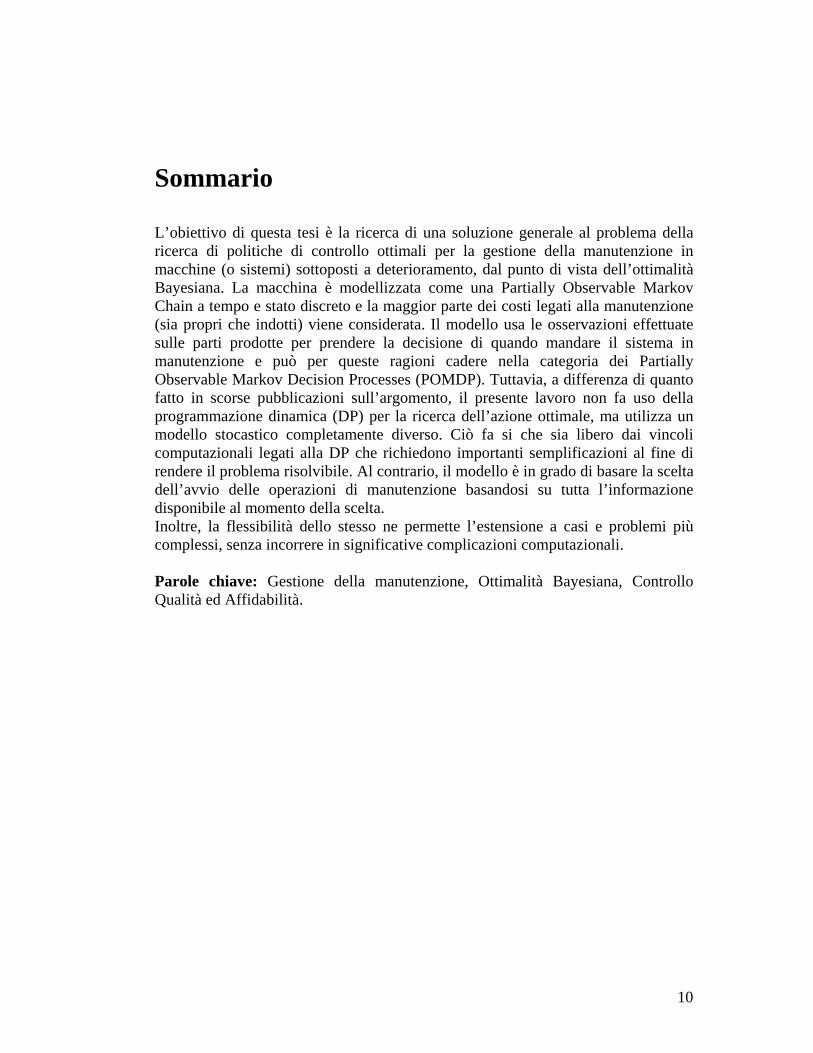
Sommario L’obiettivo di questa tesi è la ricerca di una soluzione generale al problema della ricerca di politiche di controllo ottimali per la gestione della manutenzione in macchine (o sistemi) sottoposti a deterioramento, dal punto di vista dell’ottimalità Bayesiana. La macchina è modellizzata come una Partially Observable Markov Chain a tempo e stato discreto e la maggior parte dei costi legati alla manutenzione (sia propri che indotti) viene considerata. Il modello usa le osservazioni effettuate sulle parti prodotte per prendere la decisione di quando mandare il sistema in manutenzione e può per queste ragioni cadere nella categoria dei Partially Observable Markov Decision Processes (POMDP). Tuttavia, a differenza di quanto fatto in scorse pubblicazioni sull’argomento, il presente lavoro non fa uso della programmazione dinamica (DP) per la ricerca dell’azione ottimale, ma utilizza un modello stocastico completamente diverso. Ciò fa si che sia libero dai vincoli computazionali legati alla DP che richiedono importanti semplificazioni al fine di rendere il problema risolvibile. Al contrario, il modello è in grado di basare la scelta dell’avvio delle operazioni di manutenzione basandosi su tutta l’informazione disponibile al momento della scelta. Inoltre, la flessibilità dello stesso ne permette l’estensione a casi e problemi più complessi, senza incorrere in significative complicazioni computazionali. Parole chiave: Gestione della manutenzione, Ottimalità Bayesiana, Controllo Qualità ed Affidabilità.
11
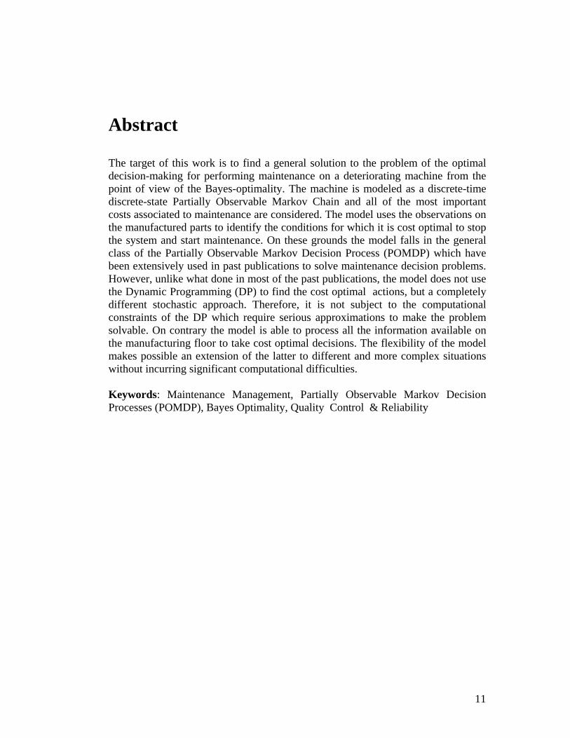
Abstract The target of this work is to find a general solution to the problem of the optimal decision-making for performing maintenance on a deteriorating machine from the point of view of the Bayes-optimality. The machine is modeled as a discrete-time discrete-state Partially Observable Markov Chain and all of the most important costs associated to maintenance are considered. The model uses the observations on the manufactured parts to identify the conditions for which it is cost optimal to stop the system and start maintenance. On these grounds the model falls in the general class of the Partially Observable Markov Decision Process (POMDP) which have been extensively used in past publications to solve maintenance decision problems. However, unlike what done in most of the past publications, the model does not use the Dynamic Programming (DP) to find the cost optimal actions, but a completely different stochastic approach. Therefore, it is not subject to the computational constraints of the DP which require serious approximations to make the problem solvable. On contrary the model is able to process all the information available on the manufacturing floor to take cost optimal decisions. The flexibility of the model makes possible an extension of the latter to different and more complex situations without incurring significant computational difficulties. Keywords: Maintenance Management, Partially Observable Markov Decision Processes (POMDP), Bayes Optimality, Quality Control & Reliability

Chapter 1
Introduction and literature review
1.1 Introduction Most of the systems used in manufacturing tend to wear, deteriorate or break. Systems used in the production of goods or for delivering services represent a significant percentage of the capital invested in most industries, and the maintenance of such systems has an extremely important role. Maintenance actions can include inspecting, repair or replace a given part of the system in order to avoid that the latter works in an undesirable condition. Working in such conditions can be very expensive, and such costs are often difficult to predict. In fact, there is a wide range of induced costs associated to a poorly maintained system: decrease in productivity costs, lack of quality costs, inefficiency costs and lack of safety costs, which commonly represent almost half of the total costs associated to maintenance [1]. However, frequent inspections, repairs, or replacements interrupt production and increase downtime as well as costs for performing maintenance. According to [2], “Because the cost of plant maintenance is second only to the cost of plant ownership, an inadequate maintenance strategy has serious financial ramifications. The underlying cost of maintenance can make or break a firm, and is an essential element of business decisions.” On these grounds, the target of a plant manager is to take optimal decisions based on this trade-off. The way such decisions are taken changes significantly according to the policy used to schedule maintenance operations. Every machine eventually fails to perform as required and when it does it is unable to manufacture acceptable parts. A possible option is to let the system work and start maintenance only when a failure or other technical problems make it completely impossible to perform the required operations. This type of approach, called corrective maintenance, is reasonable only when the frequency and the
CHAPTER 1 ___________________________________________________________________
14
impact of the failures are relatively small, but in a lot of cases this turns out to be the most costly solution [2]. An alternative approach is to use a scheduled preventive maintenance: after a machine has functioned or performed a given operation for a predetermined amount of time, it is taken down for maintenance. This solution, besides reducing the number of unexpected failures, often leads to a decrease of the maintenance costs, since the repair operations can be performed more efficiently when scheduled before. A third possibility is to perform maintenance when the machine actually needs it. That is, instead of scheduling preventive maintenance based only on operation time, and taking the machine down whether it needs it or not, the machine is observed for signs of deterioration (tool wear, drifting out of calibration, dirty nozzles) and maintenance is performed when the machine reaches a critical point, but (possibly) before it actually fails. In theory, this seems to be the best option since the maintenance operations are started when they are actually required, thus reducing wastes of time and resources. However, the problem of this approach is that in a large range of systems, it is difficult or too expensive to observe the deterioration state of a machine (or of a given component) from the outside. Examples of such systems are components of a machine that cannot be inspected because they require the system to be stopped (e.g. a drilling tool), hidden or “invisible” components (e.g. the internal surface of a pipe) or components that are too small or too complicated to be actually inspected (e.g. semiconductor). As written in [2], the inspectability of the deterioration state of the most common components of systems undergoing maintenance is likely to decrease in the future for different reasons. A solution to these problems can be found in those maintenance policies which use the output of a given system, e.g. the parts manufactured by a machine, to understand what is the deterioration state of the latter. If it is not possible to inspect a given component of a manufacturing system, it is often possible to observe characteristics of the parts produced by the machine, and infer from them its current state of deterioration. For example, while it is not possible to measure the diameter of a drilling tool without stopping the machine, it is instead possible to measure the diameter of the holes made on the manufactured parts. Even though there is not a precise analytical correlation between the diameter of the hole and the deterioration state of the tool it is possible to use statistical considerations to infer it. In many cases this is also a reasonably cheap solution which has little or no impact on the system. In fact, the quality of the manufactured parts is very often measured to separate good parts from scraps, so in most of the situations this is an information
INTRODUCTION AND LITERATURE REVIEW ___________________________________________________________________
15
which is already available and does not need the installation of additional measuring devices on the manufacturing machines. This thesis deals with optimal decision-making for a deteriorating machine whose condition cannot be observed directly. Optimality is sought in the Bayesian sense, i.e. with the target of minimizing the expected cost by choosing between two alternatives: taking the machine down for maintenance, or letting it continue operating. The machine is modeled as a discrete-time, discrete-state homogeneous Markov process whose states represent the deterioration process, i.e. the deterioration level of the machine. These states are not directly observable; however it is assumed that the quality of the manufactured parts provides information, even if imperfect, about the state of the machine, and that quality declines as the machine degrades. Thus, the overall model belongs to the class known as partially observable Markov decision processes (POMDP). In simple words, we are looking for optimal maintenance control policies based on the observations of the output of the system. Unlike what done in previous research works, in this thesis we will not use the Dynamic Programming to determine the optimal decision, but a different method based on the Renewal Processes Theory will be implemented. The reason why such different approach has been undertaken is that the Dynamic Programming (DP) techniques have important limitations which prevent them from being applied to more complex situations. In fact, in order to avoid the DP space to become dense (uncountably infinite) it is necessary to discretize the space of the observations and to consider only a limited window of the most recent observations to take the maintenance decision. Therefore, while the systems creates parts whose quality measurements is a real number, the controller of the system has to discretize such numbers and to consider only the latest observations in his decision process. This results in serious loss of information that could otherwise be used to take better decisions thus improving the performance of the system. It is important to underline that the forementioned limitations of the DP are structural and cannot be easily eliminated or overcome. For example, in most the past publications about this topic, the discretization of the observations is considered as binary (good or bad) since adding additional levels of discretization seriously increases the computational burden required by the DP algorithm (to the point of making it completely unsolvable in some cases). In this publication we seek a different approach to solve the problem which does not apply the Dynamic Programming and therefore is not subject to the listed limitations. We will show how it is possible to concentrate all the information coming out of the system (in term of real observations) in a simple vector called the
CHAPTER 1 ___________________________________________________________________
16
a posteriori probability vector, and we will develop a model to take cost optimal decisions based on it. We will eventually come up with a method that uses continuous (non discretized) observations and no windowing to take the cost optimal decision. The information coming from the manufactured parts is not manipulated or modified, but it is used entirely in the decision process. In other words we are looking for a method to take cost optimal decisions based on all the possible information available to the controller. Using all the available information coming out of the system without scrapping anything leads to better decisions, and this eventually results in higher profits.

INTRODUCTION AND LITERATURE REVIEW ___________________________________________________________________
17
1.2 Literature Review In the last decades there has been a significant interest in maintenance models of items or systems characterized by stochastic failures. There is an important number of surveys on such field of research, like [3], [4] and [5], as well as papers focusing on a specific area of manufacturing [6], [7], [8], [9], [10], [11], [12], [13] and [14]. The type of problem we deal with in this document is specifically focused on manufacturing systems producing measurable parts, with the target of finding a cost optimal control policy to take the decision to inspect, repair or replace units subject to deterioration during service. However, the developed model could be extended to other types of systems subject to deterioration. Let us consider a machine subject to deterioration which can be modeled as a discrete-time homogeneous Markov process. If the machine is working (i.e. it is not down for maintenance) it is able to manufacture a new part every time step. Moreover, at every time step a decision must be made as to whether or not to take the machine down for maintenance; if the machine is not taken down for maintenance, it continues producing parts. To begin, let us assume that the current state of the machine is directly observable. Such models are discussed in Derman [15] and Klein [16]. Derman assumes that the unit deteriorates stochastically through a finite set of states; it is inspected during each period, and a decision is made as to whether or not to replace it when it is found to be in one of a certain subset of states. This decision is based on the entire past history of the machine, including the present. In the paper, sufficient conditions are established for the existence of stationary non-randomized decision rules: under these conditions, a decision rule partitions the set of states into two subsets corresponding to the two decisions. Klein considers a model where deterioration is described by a Markov chain in which the machine state is known only upon inspection, after which the decision-maker may opt to replace the machine, maintain it, or let it run. The decision-maker also chooses the time of the next inspection. A similar model is considered in [17], where the cost function is generalized in order to consider an occupancy cost associated with each state. In [18], available control policies include the scheduling of inspections and preventive repairs such that the expected cost per unit time is minimized. A continuous-time Markov model is assumed for the machine, and costs include inspection, state occupancy, preventive repairs. A machine failure is detected immediately with a certain probability; if it is not, then it is discovered at the next scheduled inspection. A more general case concerns Markov models whose state is not directly observable, i.e. POMDPs, which are the type of models we use in this thesis.

CHAPTER 1 ___________________________________________________________________
18
Here, the current state of the system is not known exactly, and must be inferred from observations that only contain probabilistic information about the state. In other words, there are two sources of uncertainty that affect decision-making in a POMDP: not only are transitions among states random, but furthermore observations provide noisy evidence of the system state. Clearly, a POMDP reduces to an ordinary Markov decision process when the probability distributions are degenerate, i.e. when every possible observation provides perfect information about the current state of the system. In the absence of perfect information of the system state, the decision-maker can use the posterior probabilities of the states given all past observations: as shown by (Smallwood and Sondik) [19] these probabilities constitute a sufficient statistic, i.e. they contain all the relevant information available to make an optimal decision at each point in time. The problem of such approach is that, as time increases without bound the number of possible observation sequences approaches infinity even if each observation can only take a finite number of distinct values; as a result, the space spanned by the posterior probabilities becomes dense. When the number of Markov states is greater than two, searching for the optimal decision over an uncountably infinite cost space presents significant computational difficulties. This problem is resolved in [19] for the finite-horizon and addressed in [20] for the infinite-horizon case. Specifically, it is argued in [19] that when only a finite number of time periods remain, the optimal payoff function is a piecewise-linear and convex function of the current system state probabilities. With the convexity of the value function thus established, it is shown that the payoff space is partitioned into a finite number of convex regions over each of which the optimal policy is fixed. Moreover, this property can be exploited to find a simple and elegant algorithm for calculating the optimal decision policy as a linear optimization problem. The problem of the optimization of the total discounted cost over an infinite time horizon is treated by Sondik where an algorithm for the research of approximated optimal stationary policies is built. While statistical process control and preventive maintenance have each received considerable attention from researchers during the past decades, and significant progress has been made in understanding, formulating, and solving various problems in those areas, they have historically been treated as two separate problems. The problem of finding optimal control policies jointly for machine maintenance and product quality control is first addressed in [21] and [22]. The former describes a model with two basic types of maintenance policy: scheduled preventive maintenance, and maintenance on demand. Of these, the latter involves maintenance in response to signals received from the production system,
INTRODUCTION AND LITERATURE REVIEW ___________________________________________________________________
19
and decisions are thus a function of the condition of the system over time. This is extended in [22], where elements from traditional process control (control charts) are explicitly incorporated into existing maintenance models. The model is also generalized to an arbitrary number of out-of-control states and different sampling and maintenance intervals. The problem of the computational difficulties associated to the dynamic programming and the necessity of a window to the latest observations is further developed in Schick [23], where the time since the latest maintenance is also considered as an essential information to understand the state of the system, The Renewal Processes Theory, and the Renewal Reward Theorem (RRT) in particular is one of the starting points of this work; therefore a survey of the existing maintenance management models using such theory has been carried out. In general, the long run expected cost of a maintenance policy is often obtained by means of an application of the renewal-reward theorem. Barlow [24] uses the RRT to find cost optimal preventive maintenance policies, and the same approach is developed by other authors like Nguyen [25] and Wang [26] for non-perfect maintenance cases. There many other examples, often coming from different sectors (most notably the computer science), where the RRT is used to find optimal preventive maintenance policies or adaptive preventive maintenance policies. Some of them use Bayesian approaches to exploit information about the system to take cost optimal actions; examples are [27], [28], [29], [30], [31], [32]. While a large set of past publications use the RRT to find optimal preventive policies, the use of such theory for controlled systems, i.e. for systems where the decision as to whether to stop the system or not is based on the measurements of the outputs, is instead more limited. In Gosavi 2004 [33] a simulation based Learning Automata method is proposed to solve semi-Markov decision processes as an alternative to the traditional Dynamic Programming approaches. The method, however, is not based on a specific model of the system (e.g. the Markov deterioration model) and does not seek among a analytically structured set of possible optimal control policies; instead, it evaluates the effect of random actions of the controller and uses reinforcement learning techniques to gradually build a set of cost optimal actions given specific conditions of the system.

Chapter 2
Description of the model 2 We model a deteriorating machine as a discrete-time, discrete-state homogeneous Markov process (chain) composed of a sequence of states, followed by a state in which the machine is down (i.e. not producing) and needs to undergo maintenance. The most simple form of this system if represented in Figure 2.1
Figure 2.1 Model of the deteriorating Markov Chain It is very important to underline that this is the very basic structure of the Markov model of a deteriorating machine, and that a large set of modifications can be applied to this structure in order to model different situations. We will use the most simple structure of this model (the one presented in Figure 2.1) to develop our solution techniques. However, as it will be argued in the last chapter, given the solution techniques developed for this simple situation, it will be well possible to solve more complicated problems or eliminate some of the hypothesis used in this case without incurring any significant complication in the model.

DESCRIPTION OF THE MODEL ___________________________________________________________________
21
The system starts from the state one immediately after maintenance, and goes through a sequence of working states. Each of the K,...,1 working states is characterized by an increasing level of deterioration. The probability of jumping to an adjacent state during a time step is equal to p. If the system is in any of the working states, it manufactures a part every time step. We will suppose in this thesis that each manufactured part is measured, even though it would be easy to re-adapt the model in the cases where only a given percentage of parts are actually measured. When the system is in maintenance no parts are manufactured. After the state K is reached, the system can go to a “Crash” state, indicated with the letter C. This states models the last phase of the deteriorating process: the machine fails and it necessarily needs to undergo maintenance. The maintenance operations require a given amount of time, after which the system comes back to its initial state and the normal deterioration process starts again. The system is continuously supervised by a controller which has to take the decision about either stopping the system or letting it work. If the system is stopped and maintenance started because of a controller’s decision, no extra crash cost has to be paid. On the other end, if maintenance has to be necessarily started because the machine has failed, an extra cost has to be paid. This cost can model different things: the difficulty in performing the maintenance operations when they have not been planned, the damage produced by a failure to the machine, the risk associated to a crash, etc. However, ff not required, the crash cost can be eliminated.
CHAPTER 2 ___________________________________________________________________
22
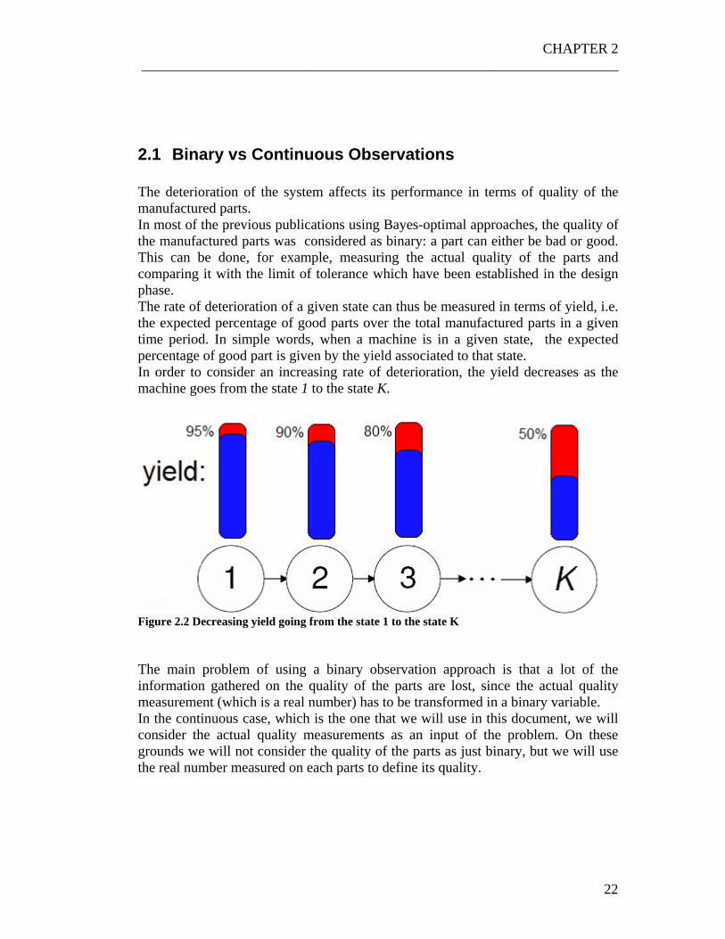
2.1 Binary vs Continuous Observations The deterioration of the system affects its performance in terms of quality of the manufactured parts. In most of the previous publications using Bayes-optimal approaches, the quality of the manufactured parts was considered as binary: a part can either be bad or good. This can be done, for example, measuring the actual quality of the parts and comparing it with the limit of tolerance which have been established in the design phase. The rate of deterioration of a given state can thus be measured in terms of yield, i.e. the expected percentage of good parts over the total manufactured parts in a given time period. In simple words, when a machine is in a given state, the expected percentage of good part is given by the yield associated to that state. In order to consider an increasing rate of deterioration, the yield decreases as the machine goes from the state 1 to the state K.
Figure 2.2 Decreasing yield going from the state 1 to the state K The main problem of using a binary observation approach is that a lot of the information gathered on the quality of the parts are lost, since the actual quality measurement (which is a real number) has to be transformed in a binary variable. In the continuous case, which is the one that we will use in this document, we will consider the actual quality measurements as an input of the problem. On these grounds we will not consider the quality of the parts as just binary, but we will use the real number measured on each parts to define its quality.
DESCRIPTION OF THE MODEL ___________________________________________________________________
23
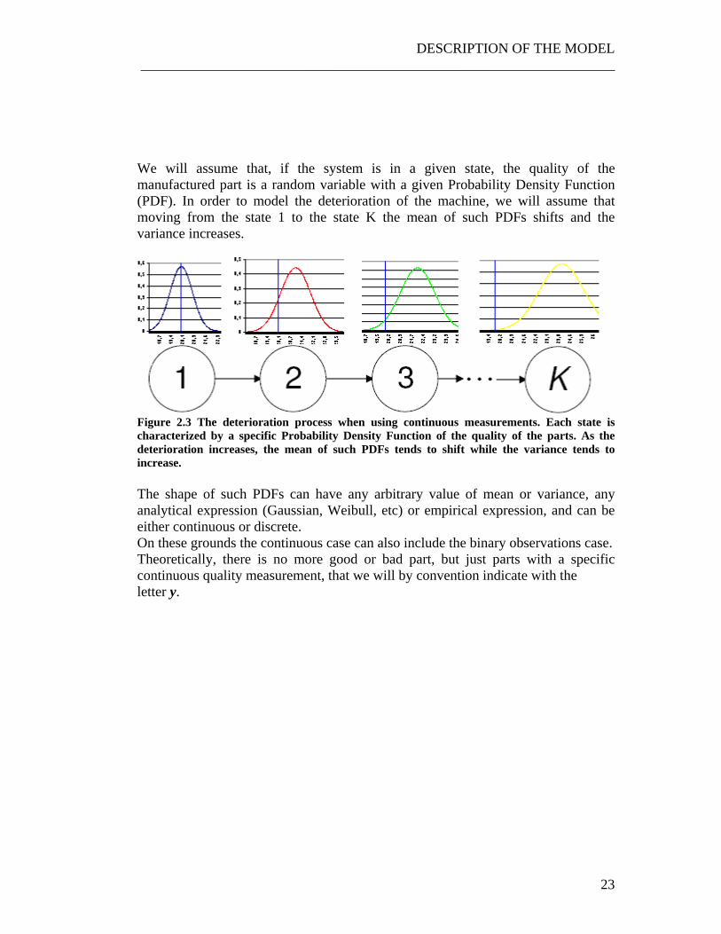
We will assume that, if the system is in a given state, the quality of the manufactured part is a random variable with a given Probability Density Function (PDF). In order to model the deterioration of the machine, we will assume that moving from the state 1 to the state K the mean of such PDFs shifts and the variance increases.
Figure 2.3 The deterioration process when using continuous measurements. Each state is characterized by a specific Probability Density Function of the quality of the parts. As the deterioration increases, the mean of such PDFs tends to shift while the variance tends to increase. The shape of such PDFs can have any arbitrary value of mean or variance, any analytical expression (Gaussian, Weibull, etc) or empirical expression, and can be either continuous or discrete. On these grounds the continuous case can also include the binary observations case. Theoretically, there is no more good or bad part, but just parts with a specific continuous quality measurement, that we will by convention indicate with the letter y.

CHAPTER 2 ___________________________________________________________________
24
2.2 The sources of cost The single machine modeled in this document is a system manufacturing parts that can be then sold in the market generating a revenue. By convention, we will consider costs to be positive: on these grounds a revenue can be considered as a negative cost. The sources of costs are listed below: Quality Costs: These are the costs required to produce a part with a given quality measurement. If the part is good and can be sold (thus generating a profit) we will consider these costs to be negative (i.e. Cost = - Generated Profit). In order to quantify the quality of a part in terms of generated profit (or lost money), we will use a cost function )(yς : this function identifies the cost for manufacturing a part with a quality dimension equal to y.
Figure 2.4 An example of a possible Cost Function of the quality of the parts. The Analytical form of the Cost Function does not affect the model, so any Cost Function )(yς can be used in the model.
DESCRIPTION OF THE MODEL ___________________________________________________________________
25
A possible Cost Function can be the one shown in Figure 2.4: the function reaches a minimum when its quality measurement is equal to a target value (in this case
21=tary ). As the quality of the part gets far from the target, the value of the part decreases. Finally, if the part measurement if out of the limit of tolerance, it can be considered as a scrap, and a cost equal to the variable cost for manufacturing it has to be paid. It is important to notice that the )(yς in Figure 2.4 is just an example and that the cost function can assume any analytical (continuous or discrete) expression without affecting the model. The simplest case of simple binary observations can be modeled considering the )(yς as being a binary function assuming different values if y: good or y: bad. Maintenance Costs: These are the costs required to perform the maintenance operations. This cost can either be constant or be a random variable. As it will be shown later, when the horizon of optimization is equal to infinite (or sufficiently long) the only
information we will require is the Average Maintenance Cost, indicated as ____MC .
Since in our model we consider infinite optimization time horizon, we will treat this value as constant. We will discuss at the end of this document how it is possible to extend the model
to those cases where ____MC is not constant, but it depends on the deterioration state of
the system. Failure Costs: As already mentioned, this is the extra cost that has to be paid if the system fails, i.e. it goes in the state C. The cost, indicated as CRASHC , keeps into consideration some factors connected to a system failure like the increase in the maintenance operations, the damage caused to the system, the risk/safety costs, etc. Opportunity Lost: These are the costs which consider the lost in productivity due to the time required to perform the maintenance operations. We will never make these costs explicit in the model (albeit an estimation of these costs is possible) but they will be indirectly present in the estimation of the Average Cost of the system. The reason why it is important to mention them is to highlight how the maintenance decision, besides the Maintenance Cost, has an indirect effect on the costs of the system due to the lost in productivity.

CHAPTER 2 ___________________________________________________________________
26
2.3 The system controller If the system is operational the system controller, after every time step, has to take the decision on either stopping the system and starting maintenance of to letting the system work. The target is to take cost optimal decisions that minimize the total cost (or maximize the total income) over a given time horizon. Given the set of costs listed before there is a clear trade-off that makes this decision difficult: if the system is stopped too soon, the impact of the Maintenance Cost and of the Lost of Productivity becomes important since the maintenance operations are performed too frequently; on the other end, if maintenance is performed too late, the quality of the parts decreases too much (because of the deterioration effect) and the risk of a failure increases as well. The Markov Process we deal with is a Partially Observable Markov Process: the controller is not able to see which is the real system state. However he can use the information connected to the measure quality of the manufactured parts to make a guess and take a decision based on such information. On these grounds the more information the system controller uses to take his decision, the better decisions he will make. This is basically the reason why we expect a continuous approach with no windowing1 to have better performance then a binary or discrete observations approach.
1 Please, see Chapter 1

DESCRIPTION OF THE MODEL ___________________________________________________________________
27
2.4 Evaluation of the parameters of the system Now that we have modeled the system the first question is: given a real system how is it possible to define the set of parameters necessary to define the Markov model? As clear, the time that the system spends in each working state and in the maintenance state is a random variable distributed as an exponential. On these grounds the working time, i.e. the total time that the machine spends in the working states before going to maintenance is a random variable given by the sum of K geometric distributions with parameter p, and therefore obeys a Pascal distribution (also known as the Pòlya and negative binomial distributions) with parameters K and p. (This is the discrete counterpart of the Erlang distribution.) Given a tool (or any deteriorating system) we would then fit the Empirical distribution of its life duration, obtained through experiments or historical data, with a Pascal distribution. The parameters K and p used in the Markov chain are those parameter that best fit such empirical distribution.
Figure 2.5 Fitting a generic Empirical distribution of the duration of a deteriorating system with a Pascal distribution. The image has been taken from [22].
CHAPTER 2 ___________________________________________________________________
28
It will be argued in the last Chapter 7.1.1 how it is actually possible to use this type of approach to fit and model through a Markov Chain almost any type of distribution of the duration of a deteriorating system. We will therefore be able the techniques developed in this document to those cases where a Pascal distribution is not a good way to model the duration of a deteriorating system. Once the parameters K and p have been found, there still the open problem of finding the Probability Density Functions of the quality of the parts associated to each state. The technique to do it is again based on the experiments or historical data gathered about the deteriorating system through which we have already evaluated the parameters K and p. A way to do so can be the following. Suppose that we have gathered data about 1,2,…h,…N tools, each of which had a total life of Nh TLTLTLTL ,....,,..., 21 time steps. This means that for the generic h-th tool, hTL observations have been gathered. Let us call hl the life of the h-th tested tool and let us take the total number of observations
hlyyy ,...,, 21 gathered for each tool and divide it in temporal order in K
groups containing an equal number of observations (i.e. K groups of Klh / ), as shown in Figure 2.6. Exploiting the linear shape of the deterioration process we can assume that (in average) the observations of the generic i-th group have been generated when the system was in the i-th state, and can thus be used to build an empirical distribution for such state. It is important to notice that this is only one of the possible ways to calculate the parameters of the problem and that other more complex and more precise methods can be applied.

DESCRIPTION OF THE MODEL ___________________________________________________________________
29
Figure 2.6 Creation of the probability density functions of the quality of the parts for the K states, starting from experimental or historical data
Chapter 3
General structure of the method 3 In this Chapter we will show how it is possible to apply the Renewal Processes Theory to find an approach alternative to the Dynamic Programming for the solution of the Markov deterioration model analyzed in Chapter 2. We will first build the basic structure of the method and progressively add new pieces that will lead to the final solution of the problem.
GENERAL STRUCTURE OF THE METHOD ___________________________________________________________________
31
3.1 The Renewal Processes Theory An important assumption of the deteriorating machine model that has been made in Chapter 2 is that each time maintenance is finished, the system is completely reset to its initial state and that so it loses every memory of what happened in the past. This assumption, which implies the hypothesis of perfect maintenance, is very useful because it lets us see each maintenance cycle as completely separate and independent from the others. The Renewal Processes Theory (RPT) is a well assessed field of the stochastic processes which studies the behavior of those system characterized by having randomly occurring instants of time during which the system returns to a state probabilistically equivalent to the starting state. Such instants are usually defined as ‘renewals’ or ‘jump times’. The mathematical properties of such systems have been satisfactorily explored in past publications and many interesting theorems have been created. A good treatment of this subject can be found on Gallager [34]. As the time elapses, different “renewals” occur. The time between two following renewals is called inter-renewal time. Since the Renewal Theory deals with stochastic processes, the inter-renewal time is a random variable. Moreover, since after every renewal the system returns to a state probabilistically equivalent to the starting state, such variables are also independent and identically distributed. An important branch of the Renewal Processes is the Renewal Reward Theory, which studies renewal processes characterized by having a random reward in each inter-renewal period depending on the length of the period itself. The Renewal Processes Theory is easily applicable to our problem: for the forementioned assumptions, maintenance can be seen as a renewal because after it is performed, the system is completely reset and so taken to a state probabilistically equivalent to the starting state. The inter-renewal time in this case is the time between two successive maintenances, i.e. the sum of the Working time and the Maintenance time (see Figure 3.1). We will call each inter-renewal time as Maintenance Cycle. The length of a Maintenance Cycle is so given by the sum of the Working and the Maintenance time of that cycle. The decision to make each new cycle start with the Working phase or with the Maintenance phase is totally arbitrary. Both the Maintenance and the Working time are random variables. We will not make any assumption about the probability density function of such variables since, as we will show in the following pages, the only thing we will need is their

CHAPTER 3 ___________________________________________________________________
32
Figure 3.1 The maintenance problem seen as a renewal process. expected value. The inter-renewal time, or Maintenance Cycle length, is a random variable as well, given by the sum of these two variables. Looking at our problem, it is easy to see that it can be described as a Renewal Reward Process. During each Maintenance Cycle, a given amount of money is gained or lost according to the quality of the produced parts, a given amount of money is certainly lost to perform maintenance and there is also a probability that the system may crash thus implying an additional Crash cost. From now on, we will only talk about costs, i.e. we will use negative costs to refer to revenues. Given the structure of the model we built, the cost gained during a Maintenance Cycle is a random variable, since the quality of the produced part is a random variable and because the failure of the machine, which implies a Crash cost, is a random event too. As we will see in the following pages, the possibility to apply the Renewal Reward Theory, and the Renewal Reward Theorem in particular, provides us with a powerful tool to simplify the problem.
3.1.1 The Renewal Reward Theorem An essential theorem of the Renewal Processes Theory is the Renewal Reward Theorem (RRT) which states that: Let R(t) be a renewal reward function for a renewal process with expected inter-renewal time E[T]= T . If T < ∞ , then with probability 1 :

GENERAL STRUCTURE OF THE METHOD ___________________________________________________________________
33
AR = ∫ =∞→=
t
tT
REdRt 0 _
][)(1limτ
ττ
( 3.1 )
where R is the reward accumulated during a generic inter-renewal period, while E[R] is its expected value. The Table 3.1 shows a key to the meaning of the variables. Table 3.1 List of the variables and functions used in the RPT
Variable Description
Variable Name
AR Average Reward
T Inter-renewal time
T Average inter-renewal time
R(t) Reward function
E[R] Expected Accumulated Reward
It is very important to notice that, while the quantity at the left of the equation requires the knowledge of the dynamic of the system over an infinite time horizon, the variables on the right side refer only to one single inter-renewal period. In simple words what this theorem says is that, for a Renewal Reward Process, it is enough to understand what happens during one single period to know the Average Reward of the system over an infinite time horizon. Such simplification becomes extremely useful in those cases like ours, where the Average Reward represents an important value of the system, whose optimization and improvement is the basic target of a policy designer.
CHAPTER 3 ___________________________________________________________________
34
3.2 Application of the RRT to the solution of the problem In this Chapter we will show how it is possible to apply the RRT for the solution of the problem. We will also underline why this is so important and we will give a hint of how this can be used in order to find an optimal control policy. The reward function in our case is a cost function C(t) , the T is the length of the generic Maintenance Cycle, while E[C] is the Expected Cost of a Maintenance Cycle. The Renewal Reward Theorem can thus be re-written as:
AC = ∫ =∞→=
t
tT
CEdCt 0 _
][)(1limτ
ττ
( 3.2 )
The integral at the left side of the equation is what is usually called the Average Cost of the system: given a large enough time horizon during which the system is run, this is the cost per time step that can be expected. It is important to underline how important such quantity is: it defines the average cost that is needed to run the system for a given time unit, or realistically speaking, the revenues that can be generated by running the system over the same time unit. Given a set of different system configurations, the system designer will choose the one with the lowest Average Cost. Identically, given a set of different maintenance policies, the plant manager will choose the one with the lowest Average Cost. The power of this theorem is that it lets us find this important value, which depends on what happens in this system during an infinite time horizon (or realistically speaking, during its whole life cycle) concentrating the attention on one single Maintenance Cycle. The solution of the problem can now be narrowed down to the search of the Average Length of a Maintenance cycle T and the Expected Cost of a maintenance cycle E[C]. Our concentration in the next sections will thus be focused on the method to find these two values. We will first analyze the Average Time and then the Expected Cost.
3.2.1 Calculation of T , the Average Length of a Maintenance Cycle As shown in the Figure 3.1 the length of a Maintenance Cycle is given by the contribution of the Working Time and the Maintenance Time MTWTT += .
GENERAL STRUCTURE OF THE METHOD ___________________________________________________________________
35
For the hypothesis of our core problem, the Maintenance and the Working time are not correlated and so the Average Length of a Maintenance Cycle is simply given by:
______MTWTT +=
( 3.3 )
We will discuss in the Subsection 7.1.2 how it is possible to relax this hypothesis. The Maintenance Time, which in most cases is a random variable, depends on how maintenance is organized in a given manufacturing context where the machine is
working. We will therefore take the ____MT as an input variable of the problem.
The Average Working Time is also a random variable: this is the time that the machine spends working (and manufacturing parts) after the last maintenance has been finished. For the way the problem has been formulated, we are dealing with a discrete time problem, where the time step is equal to the reciprocal of the production rate of the machine when it is operational. On these grounds, we will always consider the time as discrete. However, the results presented in this chapter can be easily extended to a continuous case . Let us call n the time since the system has started to work after a maintenance and )(nwt the discrete probability distribution function of the Working Time. Please note that, as n represents the time since the system has started to work after the last maintenance, all the probabilities that will be used in the following pages and which are function of n, are automatically conditioned on the fact that the system has not undergone maintenance yet since the beginning of the new maintenance cycle. The function )(nwt defines the probability that the system is stopped (for a failure or for a controller’s decision) at a time step n. We can thus find the expected value of the working time as:
∑∞
==
1
_____)(
nnwtnWT
( 3.4 )
Let us call )(nps the discrete Cumulative Distribution Function of )(nwt , i.e. the probability that the system is stopped before a time step n (the name ps stands for probability of stopping).
Using a well known result of the probability theory, ____WT can also be rewritten as:

CHAPTER 3 ___________________________________________________________________
36
∑∞
=−=
1
____))(1(
nnpsWT
( 3.5 )
For a non-controlled system, i.e. for a system where maintenance is performed only if a failure occurs, )(nps is simply the probability that a failure has occurred before a time n. In the case of a controlled system, i.e. a system that can be stopped to perform maintenance according to a specific control policy based on the quality of the parts, )(nps should also consider the probability that the system controller decides to stop the system and perform maintenance before a time n. It is also possible to consider the case where a Periodic Maintenance policy is applied: in this case, after a given time WTL (Working Time Limit), the system is stopped regardless of what happened in the meantime. In this case the Equation ( 3.5 ) becomes:
∑ =−=
WTL
nnpsWT
0
____))(1(
( 3.6 )
i.e. there is always a limit WTL to the Length of the Working Time. In general, it is preferable to consider such limit in the equation of the Average Working Time, even if a Periodic Maintenance is not being used without loss of generality (if WTL is infinite we get the Equation ( 3.5 )). For example, there might be situations where, even though the Maintenance decision is given by a specific control policy based on the quality of the parts, the system is stopped anyway after a given time WTL. (e.g. mandatory periodic maintenance). Moreover, as we will show in the following chapters, the limit WTL can be exploited to reduce the computational complexity of the problem, introducing a very small but useful approximation. Therefore, from now, we will always consider this time limit. The definition and the calculation of the functions ps(n) for our problem will be discussed in detail in the following chapters.
3.2.2 Calculation of the Average Cost of a Maintenance Cycle E[C] The Expected Cost of a Maintenance Cycle should consider the three sources of costs used in our model:
GENERAL STRUCTURE OF THE METHOD ___________________________________________________________________
37
• Production costs: i.e. cost for manufacturing parts. These costs can also be negative when the manufactured parts generate a revenue.
• Maintenance costs: cost for performing maintenance • Failure Costs: additional costs due to failures . These costs are connected to
the Crash Cost and to the probability that a crash occurs during a maintenance cycle.
On these grounds we have:
_____][][][ MCCECECE FAILUREPROD ++=
( 3.7 )
Let us analyze these contributions individually. Production Costs: Let us create a function c(n) defining the expected production cost for generating a part at a time step n. We will show later how to calculate such cost. Let us also create function )(nC , which defines the total expected cumulative production cost of a system which has been running for n time steps after the last maintenance. In other words, if a failure occurs or if the controller stops the system after n time steps, the total expected accumulated cost for manufacturing parts is C(n). For the way it has been defined, )(nC can be calculated as:
∑=
=n
i
ncnC1
)()( ( 3.8 )
Now, the Expected Production cost can be calculated integrating )(nC over the probability function of the duration of the Working Time )(nwt . We thus get:
∑∞
==
1)() (][
nPROD nwtnCCE
( 3.9 )
Similarly to what done for the Equation ( 3.5 ), it can be proved (Appendix II) that the Equation ( 3.9 ) can be rewritten as:
∑∞
=−=
1))(1) ((][
nPROD npsncCE
( 3.10 )

CHAPTER 3 ___________________________________________________________________
38
Intuitively, what we are doing is to weight the expected cost of each time step with the probability that the system will actually go through that time step. Writing the expected value of the production cost and of the working time length as a function of )(nps rather then of )(nwt will be useful to get to a simpler solution for the Markov deterioration model. As already mentioned, c(n) is an expectation: the cost of a part which is manufactured after n time steps is not deterministic but it depends on the quality of that part. Since the quality of the parts is always a random variable, the cost of that time step is a random variable as well. We can calculate this expectation building a probability density function of the quality of the parts y manufactured at the time step n. We will call this function
)|( nyf , i.e. the probability density function of y conditioned by the time n. If we create a Quality Cost Function )(yς , i.e. a function which defines the cost for producing a part with a quality measurement y, then we can build the cost function c(n) as an integral:
∫∀
=y
dynyfync ) |()()( ς ( 3.11 )
Where y∀ mean the range of all the possible values of y, for example if the quality of the parts can only be positive then ],0[ +∞∈y . The Equation ( 3.10 ) hence becomes:
∑ ∫=∀ ⎥
⎥⎦
⎤
⎢⎢⎣
⎡−=
WTL
ny
PROD dynyfynpsCE0
)|()())(1(][ ς
( 3.12 )
The problem of the calculation of both )(nps and )|( nyf will be discussed afterwards. Failure Costs: As already mentioned in the Chapter 2, in our model we consider the possibility of a Crash Cost ( crashC ), i.e. of an additional cost that the plant manager have to pay if a failure occurs. The average failure cost is the cost that the plant managers have to pay (in average) for each maintenance cycle because a crash event has happened.
GENERAL STRUCTURE OF THE METHOD ___________________________________________________________________
39
Intuitively, the burden of the failure costs are strictly correlated to the probability that such event may occur and to the entity of the Crash Cost. Calling CRASHP the probability that a crash event may take place during a maintenance cycle, the expected failure cost is simply given by:
crashCRASHFAILURE CPCE ][ = ( 3.13 )
Now, if we define )(npcrash , the probability that a crash event occurs exactly after n time steps since the last maintenance, the Equation ( 3.13 ) can easily be re-written as:
∑ ==
WTL
n crashcrashFAILURE npCCE0
)( ][ ( 3.14 )
Intuitively, for a deteriorating system the likelihood that a crash event occurs should increase with the time and so the function )(npcrash should be monotonic increasing. We will show in the following chapters how )(npcrash can be simply calculated for our problem. Maintenance cost
As already said for the maintenance time, the Average Maintenance Cost _____MC is
constant and is taken as an input value of the problem. The fact that both the maintenance time and cost are constant implies that maintenance operations are the same regardless of the state of deterioration of the system when the maintenance is performed. This situation is typical of those cases when the repair operations are standard (e.g. Change tool, Change component). However, there are more complex situations where both the Maintenance Time and the Maintenance Cost can change according to the state of deterioration. For example the deterioration can make the repair operations more complex or longer (e.g. Cleaning an oxidized surface, cleaning a nozzle or overhauling a tool becomes more complicated if this items are more deteriorated). We will explain how to extend the model to these situations at the end of this document. The total Expected Cost of a Maintenance cycle hence becomes:
CHAPTER 3 ___________________________________________________________________
40
_____
0)( ) () ())(1(][ MCnpCdyyYynpsCE WTL
ny
crashCRASHn +⎥⎥⎦
⎤
⎢⎢⎣
⎡+−=∑ ∫=
∀
ς
( 3.15)
In the Table 3.2 the variables and functions used in this Subsection are shown in schematic way. The most important functions that will be used in the following chapters have been marked with a red asterisk.

GENERAL STRUCTURE OF THE METHOD ___________________________________________________________________
41
Table 3.2 Summary of the variables and function used in this chapter. The ones marked with the red asterisk are the most important and will be used in the following chapters.
Variable symbol
Variable Name Description
* AC Average Cost ∫ =∞→
t
tdC
t 0)(1lim
τττ
WT Working Time Time spent producing part during a Maintenance Cycle
MT Maintenance Time Time spent performing maintenance during a Maintenance Cycle
* ____MT
Average Maintenance Time It is an input value
*
y Measurement of the Quality of the parts
* n Time since last maintenance
*
WTL Working Time Limit Decided by the Control Policy designer or used to simplify the computational
complexity of the problem ];0] +∞∈WTL
T Length of a generic Maintenance Cycle
WT + MT
)(nwt Probability function of the duration of the Working Time WT
*
)(nps Cumultative distribution function of )(nwt or probability that the system is
stopped before a time n
)(yς Quality Cost Function Cost for producing a part with a Quality Measurement y
)|( Nyf Probability Density Function of the Quality of the parts at a time step n (if the system is still working)
* )(npCRASH Probability of a Crash event at the time step n
*
____WT
Average Working Time ∑ −WTL nps0
))(1( * T Maintenance Cycle Average Length ________
MTWT + *
E[C]
Expected Cost of a maintenance cycle

CHAPTER 3 ___________________________________________________________________
42
3.2.3 Finding the Optimal Control Policy: an outline of the method With the equations ( 3.6 ) ( 3.3 ) and, we are able to calculate both the Average Length of a Maintenance Cycle T and the Expected Cost of a Maintenance Cycle
][CE , which means that we can calculate the Average Cost of the system. Most of the numbers and functions of the Table 3.2 are just input values of the problem. Only the functions )(nps , )(yYn , )(npCRASH have to be somehow calculated and they all depend on the control policy that is being used. Before continuing we remind briefly the variables used and discusses in the Chapter 2 that will be used in the following pages:
• K = Number of working states of the Markov Chain of the deteriorating system
• )(yfi = Probability density function of the quality of the parts of the generic state i
• p = Probability of transition between two adjacent states in the Markov Chain of the deteriorating system
• P = Transition probability matrix of the Markov Chain of the deteriorating system
All these parameters, together with the Average Maintenance Time ____MT , the
Average Maintenance Cost _____MC , the Quality Cost Function )(yς , the Crash Cost
CrashC are input values of the problem. In other words, these parameters define the problem.
GENERAL STRUCTURE OF THE METHOD ___________________________________________________________________
43
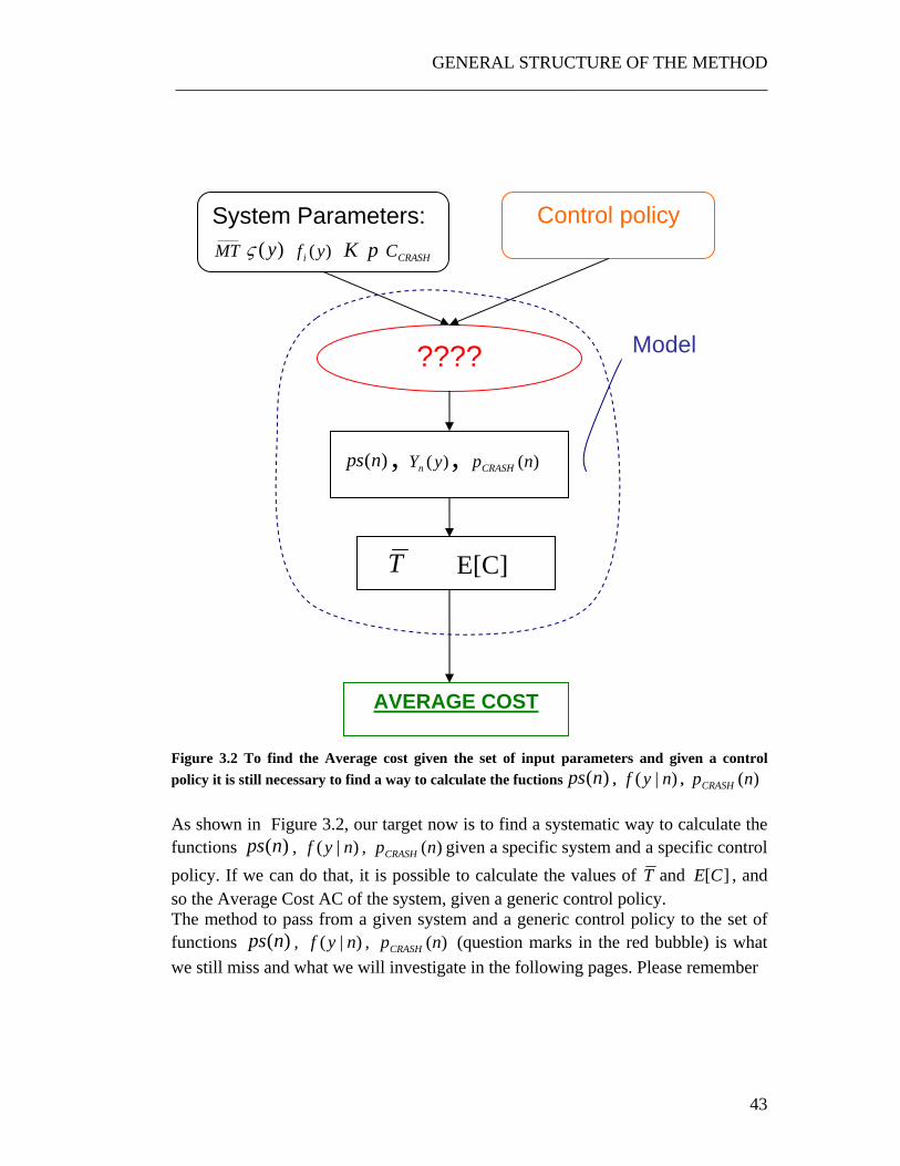
Figure 3.2 To find the Average cost given the set of input parameters and given a control policy it is still necessary to find a way to calculate the fuctions )(nps , )|( nyf , )(npCRASH
As shown in Figure 3.2, our target now is to find a systematic way to calculate the functions )(nps , )|( nyf , )(npCRASH given a specific system and a specific control policy. If we can do that, it is possible to calculate the values of T and ][CE , and so the Average Cost AC of the system, given a generic control policy. The method to pass from a given system and a generic control policy to the set of functions )(nps , )|( nyf , )(npCRASH (question marks in the red bubble) is what we still miss and what we will investigate in the following pages. Please remember
System Parameters: ____MT )(yς )(yfi K p CRASHC
????
Control policy
T E[C]
AVERAGE COST
)(nps , )(yYn , )(npCRASH
Model
CHAPTER 3 ___________________________________________________________________
44
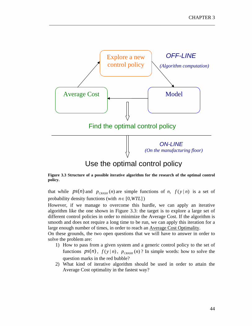
Figure 3.3 Structure of a possible iterative algorithm for the research of the optimal control policy. that while )(nps and )(npCRASH are simple functions of n, )|( nyf is a set of probability density functions (with ],0[ WTLn ∈ ) However, if we manage to overcome this hurdle, we can apply an iterative algorithm like the one shown in Figure 3.3: the target is to explore a large set of different control policies in order to minimize the Average Cost. If the algorithm is smooth and does not require a long time to be run, we can apply this iteration for a large enough number of times, in order to reach an Average Cost Optimality. On these grounds, the two open questions that we will have to answer in order to solve the problem are:
1) How to pass from a given system and a generic control policy to the set of functions )(nps , )|( nyf , )(npCRASH ? In simple words: how to solve the question marks in the red bubble?
2) What kind of iterative algorithm should be used in order to attain the Average Cost optimality in the fastest way?
(Algorithm computation)
Explore a new control policy
Model Average Cost
Find the optimal control policy
OFF-LINE
Use the optimal control policy
ON-LINE (On the manufacturing floor)
GENERAL STRUCTURE OF THE METHOD ___________________________________________________________________
45
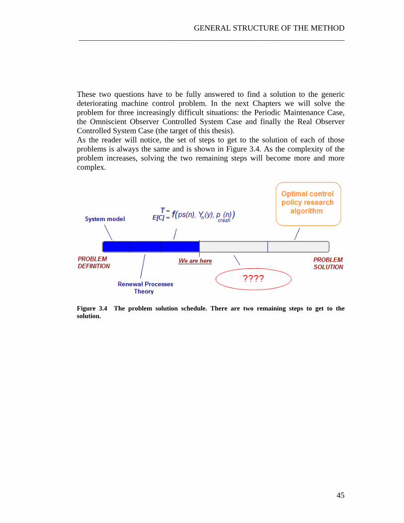
These two questions have to be fully answered to find a solution to the generic deteriorating machine control problem. In the next Chapters we will solve the problem for three increasingly difficult situations: the Periodic Maintenance Case, the Omniscient Observer Controlled System Case and finally the Real Observer Controlled System Case (the target of this thesis). As the reader will notice, the set of steps to get to the solution of each of those problems is always the same and is shown in Figure 3.4. As the complexity of the problem increases, solving the two remaining steps will become more and more complex.
Figure 3.4 The problem solution schedule. There are two remaining steps to get to the solution.

CHAPTER 3 ___________________________________________________________________
46
3.3 A useful example: the Periodic Maintenance case To better understand how to apply the described method and how to solve the two open questions shown at the end of the previous section, we will focus on a simple but important situation: the Periodic Maintenance Case. The purpose of this section is not to be just a trivial application of what has already been explained. On contrary, the results and the methods that are developed in the following pages will be used as a starting point for the solution of more complex problems. We will solve the problem completely, solving the two missing steps and thus getting to the right end of the bar shown in Figure 3.4, i.e. to the problem solution. The solution of more complex situations, like the Controlled System Case, will not be as easy, but with this simple example it will be easier to understand. The Periodic Maintenance is a type of policy based on performing maintenance after a given period of time, regardless of what happened in the system in the meantime. With this approach, the quality of the manufactured parts does not affect the controller’s decision, who will simply start maintenance if the system gets broken or after a pre-defined number of time steps since the last maintenance. On these grounds there is just one degree of freedom in the control policy, i.e. the number of time steps after which the system has to be cyclically stopped.
3.3.1 Model of the single maintenance cycle As already said, the great advantage of the Renewal Processes Theory is that it simplifies the problem, making possible to focus on one single maintenance cycle instead of looking at the entire history of the system over an infinite time horizon. The functions )(nps , )|( nyf , )(npCRASH are all referred to a single maintenance cycle, because they depend on a variable n which is the discrete time since the last maintenance. On these grounds, we will need to find a new way to model the single maintenance cycle of the deteriorating machine. This is simple to find: what we need to do is to take the Markov chain of the deterioration model in Figure 2.1 and erase the arrow from the Maintenance state to the first states.

GENERAL STRUCTURE OF THE METHOD ___________________________________________________________________
47
Figure 3.5 Markov chain model of a single maintenance cycle What we get is shown in Figure 3.5: when maintenance is completed, the system starts from the state 1. As the time elapses, the system gradually goes to the maintenance state. There is no possibility to skip from the maintenance state to the first state because we are modeling the single maintenance cycle. It is important to understand exactly what we are doing, because it is simple to get confused at this point. In particular it is important to fully understand how the meaning of the M state changes in this case. The Figure 3.6 can help understand this concept. As deductible from the Markov chain in Figure 3.5, after a long enough period of time, the probability to be in the maintenance state gets higher and higher. The reason for this is that, taken a deteriorating system, the probability that it has undergone maintenance after a long time becomes high. We are not saying that, taken a deteriorating machine, after a long period of time the probability to be in the maintenance state approaches 1. Since we are now modeling the single maintenance cycle, we are simply stating that after a long enough period of time, the probability that the system has gone in the maintenance state at least for one time approaches 1.

CHAPTER 3 ___________________________________________________________________
48
Figure 3.6 Global time vs local time. With the renewal processes theory we study the system focusing on one single maintenance cycle. This requires to pass from a global time vision to a local time, and so to pass from the original Markov Chain deterioration model to the one represented in Figure 3.5. Identically the probability of the states 1,2,….,K defines the probability that the system is any of those states after a given time has elapsed since the last maintenance. If a long time has elapsed, it is very unlikely that the system will be in any of the working state, and it is instead likely that it has undergone maintenance at least for once and that a new maintenance cycle has begun. It is important to remember that the state C, like in the original model, refers to the Crash State, M is the maintenance state and K is the total number of working states of the system (with deterioration rate increasing from 1 to K). Let us now define the probability vector:
[ ])(),(),(),....,2(),1( MCK nnnnnn ππππππ = ( 3.16 )

GENERAL STRUCTURE OF THE METHOD ___________________________________________________________________
49
i.e. the time dependent vector with the values of the probabilities of being in one of the states. This vector can be built and calculated before the system is run, because it does not depend on the observations of the manufactured parts (it depends on the theoretical dynamic of the system described by deteriorating machine Markov Chain). For the hypothesis of perfect maintenance, we can also initialize such vector:
[ ]== )(),(),(),....,2(),1( 000000 MCK ππππππ
]000....01[=
( 3.17 )
Let us also write the transition probability matrix of the Markov Chain in Figure 3.5. We will indicated it with the symbol P and we will call it Natural Transition Probability Matrix, because it is referred to the Markov chain of the natural deterioration of the system, i.e. with no type of control.
⎥⎥⎥⎥⎥⎥⎥⎥
⎦
⎤
⎢⎢⎢⎢⎢⎢⎢⎢
⎣
⎡
−
−−
=
1............010.........0010....................0...0100......01
pp
pppp
P
( 3.18 )
We now have all the tools to solve the problem.
3.3.2 Solving the red bubble: research of the functions )(nps , )|( nyf , )(npCRASH .
We will now show how it is possible to find an expression for this set of functions given the model of the Deteriorating Markov chain that we are using. We will show how to find these three variables separately.
CHAPTER 3 ___________________________________________________________________
50
Research of the )(npCRASH The probability vector nπ at a given time n can be easily found given with the equation:
nn P⋅= 0ππ
( 3.19 )
If we know the probability vector at a given time n, then we can immediately find the probability )(npCRASH since:
)()( Cnp nCRASH π= ( 3.20 )
Research of the )(nps Similarly, the probability )(nps , i.e. the probability that the system is stopped and maintenance is performed before the time n is given by the sum of the Crash and the Maintenance state:
)()()( MCnps nn ππ += ( 3.21 )
Research of the )|( nyf The set of functions )|( nyf are the probability density functions of the quality of the parts, conditioned by a time step n. The question that we are trying to answer in this case is: if the system is still working after n time steps, what is the probability density function of the quality of the manufactured parts? This function depends on the probability density functions of the quality of the parts )(yfi of each of the K states and on the probability of being in any of those states. What we need to find first is the probability of being in any of the K states at a time n, given that the system is still working after n time steps. This is the conditional probability that the system is in a generic working state ],1[ Ki ∈ , given that it is still working after n time steps.
GENERAL STRUCTURE OF THE METHOD ___________________________________________________________________
51
If we call:
)(iAn = probability to be in the working state ],1[ Ki ∈ at a time step n
nB = probability that the system is still working after n time steps )(inρ = conditional probability that if the system is still working after n time step, it
is in the generic working state ],1[ Ki ∈ We can write the Bayes theorem:
)(inρ = )|)(( ni BnAP = )(
))(()) (|(
n
iin
BPnAPnABP
Now we know that:
• ))(( nAP i = )(Cnπ , i.e. the probability to be in the generic state i at a time n • )( nBP = ))(1( nps− , i.e. the probability that the system is still working after
n time steps • ))(|( nABP in = 1. In fact, if the system is in a working state, we know with
probability 1 that it is still working. On these ground we have that:
==)())((
)(n
in BP
nAPiρ
))(1()(nps
in
−π
( 3.22 )
The function )|( nyf can be now calculated by the sum of the K probability density functions of the quality of the states )(yfi , weighted with the probability of being in one of those states
)()(..)()(..)()()|( 11 yfnyfnyfnNyf KKii ρρρ ++++= ( 3.23 )
Given the Equations ( 3.20 ), ( 3.21 ) and ( 3.23 ) we can now rewrite the Equations of the Average Cost of a Maintenance Cycle and Average Length of a Maintenance Cycle as:
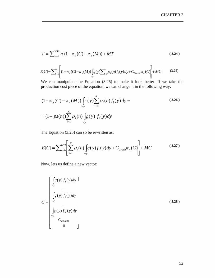
CHAPTER 3 ___________________________________________________________________
52
_____
1
__))()(1 ( MTMCnT WTL
n nn +−−= ∑ =ππ
( 3.24 )
_____
0 1)( )()()())()(1(][ MCCCdyyfnyMCCE WTL
ny
nCrashK
i iinn∑ ∫ ∑=∀
=+
⎥⎥⎦
⎤
⎢⎢⎣
⎡+−−= πρςππ
(3.25)
We can manipulate the Equation (3.25) to make it look better. If we take the production cost piece of the equation, we can change it in the following way:
dyyfynnps
dyyfnyMC
iy
K
ii
y
K
iiinn
) () ()())(1(
)()()())()(1(
1
1
∫∑
∫ ∑
∀=
∀ =
−=
=−−
ςρ
ρςππ
( 3.26 )
The Equation (3.25) can so be rewritten as:
_____
01
)() ()()(][ MCCCdyyfynCE WTL
ny
nCrashi
K
ii +
⎥⎥⎦
⎤
⎢⎢⎣
⎡+= ∑ ∫∑=
∀=
πςρ
( 3.27 )
Now, lets us define a new vector:
⎥⎥⎥⎥⎥⎥⎥⎥⎥⎥⎥
⎦
⎤
⎢⎢⎢⎢⎢⎢⎢⎢⎢⎢⎢
⎣
⎡
=
∫
∫
∫
∀
∀
∀
0
) () (...
) () (...
) () ( 1
CRASH
yK
yi
y
C
dyyfy
dyyfy
dyyfy
C
ς
ς
ς
( 3.28 )

GENERAL STRUCTURE OF THE METHOD ___________________________________________________________________
53
The vector C does not depend on any time index, so it has to be calculated only on time at the beginning of the algorithm. We can now modify the Equation ( 3.27 ), introducing the vector C and finally get to a very simple structure:
[ ] _____
0][ MCCCE WTL
n n +⋅= ∑ =π
( 3.29 )
The interpretation of this equation is the following: the C vector can be seen as a state cost vector, i.e. a vector containing the expected cost for being in one of the states for one time step. Multiplying this vector for the state probability vector at given time n we get the value of the step cost at time n. Summing all these costs and adding the Maintenance Cost we eventually get the expected cost of a maintenance cycle.
3.3.3 Finding the optimal control policy Now that we have found how to calculate the three functions )(nps , )(yYn ,
)(npCRASH there is still an open problem: the research of the optimal policy. In a Periodic Maintenance we do not have many degrees of freedom: the only thing that can be changed is the number of time steps after which maintenance is performed. In the previous equations we have called this limit WTL (Working Time Limit) which is one of the parameters of the Equations ( 3.24 and (3.25). A possible approach is an iterative algorithm which gradually changes WTL and uses the Equations ( 3.2 ), ( 3.24 and (3.25) to find the Average Cost associated to each value. If a large enough range of values of WTL are explored ( ],1[ maxWTLWTL ∈ ) we can find what is the values which minimizes the Average Cost of the system. A sketch of this approach is shown in Figure 3.7: as clear, we have used the same structure of the general method shown in Figure 3.3 and adapted to the particular Periodic Maintenance case.
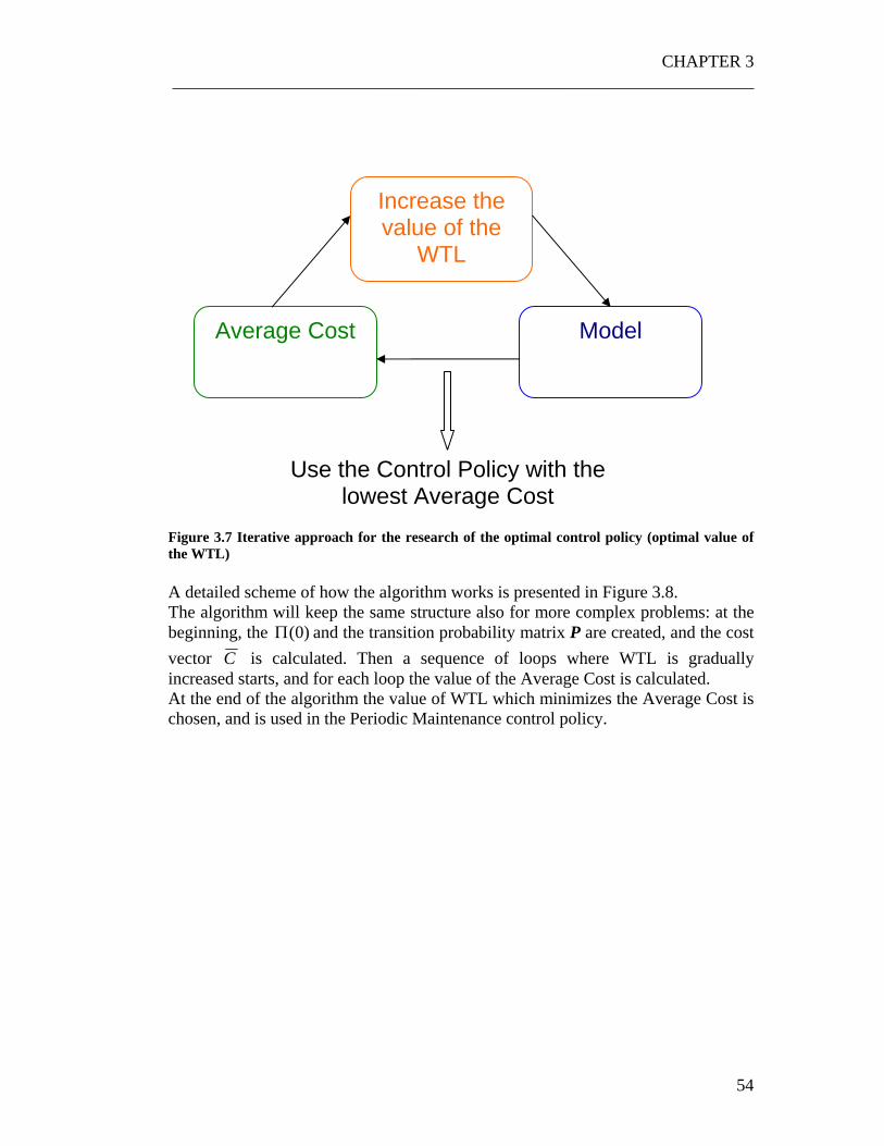
CHAPTER 3 ___________________________________________________________________
54
Figure 3.7 Iterative approach for the research of the optimal control policy (optimal value of the WTL) A detailed scheme of how the algorithm works is presented in Figure 3.8. The algorithm will keep the same structure also for more complex problems: at the beginning, the )0(Π and the transition probability matrix P are created, and the cost vector C is calculated. Then a sequence of loops where WTL is gradually increased starts, and for each loop the value of the Average Cost is calculated. At the end of the algorithm the value of WTL which minimizes the Average Cost is chosen, and is used in the Periodic Maintenance control policy.
Increase the value of the
WTL
Model Average Cost
Use the Control Policy with the lowest Average Cost
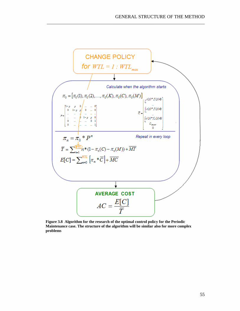
GENERAL STRUCTURE OF THE METHOD ___________________________________________________________________
55
Figure 3.8 Algorithm for the research of the optimal control policy for the Periodic Maintenance case. The structure of the algorithm will be similar also for more complex problems

CHAPTER 3 ___________________________________________________________________
56
3.3.4 A case with real numbers In order to complete this section it is interesting to see a practical application of the explained model for a real case. We will study a system which deteriorates in 4 states.
The starting data of the problem are:
• Number of states K=4
• Average Maintenance Cost ____MC = 1000
• Average Maintenance Time ____MT = 20 (time steps)
• Distribution of the Quality of the Parts of the four states: Gaussian, with mean and variance listed in the chart below
• Cost function )(yς , i.e. cost for manufacturing a part with quality measurement y, shown in Figure 3.10. The cost increases parabolically as y goes far from the target value (21). When y is out of the acceptability range, i.e. when 23 18 >∨< yy the part is a scrap and =)(yς part variable costs (the part manufacturer loses an amount of money equal to the variable cost for manufacturing the part).

GENERAL STRUCTURE OF THE METHOD ___________________________________________________________________
57
16 18 20 22 24 26 280
0.1
0.2
0.3
0.4
0.5
0.6
0.7
0.8
y
Probability Density Function of the quality of the parts
State 1State 2State 3State 4
Figure 3.9 Probability density function of the quality of the parts for the 4 states used in this example. Please note how the mean of the functions shifts while the variance increases. Table 3.3 List of the mean and variance of the probability density functions of the quality of the parts for the four states
State Mean Variance 1 20 0.5 2 21 0.75 3 22 1 4 23 1.25
Table 3.4 List of the variables of the model and their values
Variable Value K 4 p 0.03

CHAPTER 3 ___________________________________________________________________
58
_____MC
1000 _____MT
20
CRASHC 2500
Figure 3.10 An hypothetical cost function, i.e. cost for manufacturing a part with a quality measurement y Running the algorithm in Figure 3.8 we get the graph of the Average Cost of the system as a function of the Working Time Limit (WTL). The result is shown in Figure 3.11.

GENERAL STRUCTURE OF THE METHOD ___________________________________________________________________
59
0 100 200 300 400 500 600-10
0
10
20
30
40
50
60
70
WTL
Ave
rage
Cos
tMC=1000; MT=20
Figure 3.11 Average Cost as a function of the WTL As clear, the Average Cost starts from a very high values, it reaches a minimum and then keeps increasing until reaching an asymptotic value. This can be explained in the following way: if the periodic maintenance is scheduled after a limited number of time steps, the machine spends a too long time and too much money to perform maintenance, and only a small fraction of the Maintenance Cycle is used to produce parts. As the WTL increases more time is devoted to manufacture parts, and this increases the revenues that can be generated, thus decreasing the Average Cost of the system. However, there is a limit point after which the AC starts increasing again: if maintenance is scheduled after a too long time, too many bad parts are produced and the likelihood that the system crashes increases as well. As WTL keeps increasing, the AC stabilizes to a fixed value: in fact, if the periodic maintenance is scheduled after an extremely long time, maintenance is very likely to start because a crash has occurred, so the choice of a different value of WTL does not affect the AC of the system. We can so find the value of WTL which optimizes the Average Cost. In this case we can get an optimal (minimum) Average Cost of 72.12−=optAC for a 59=optWTL .
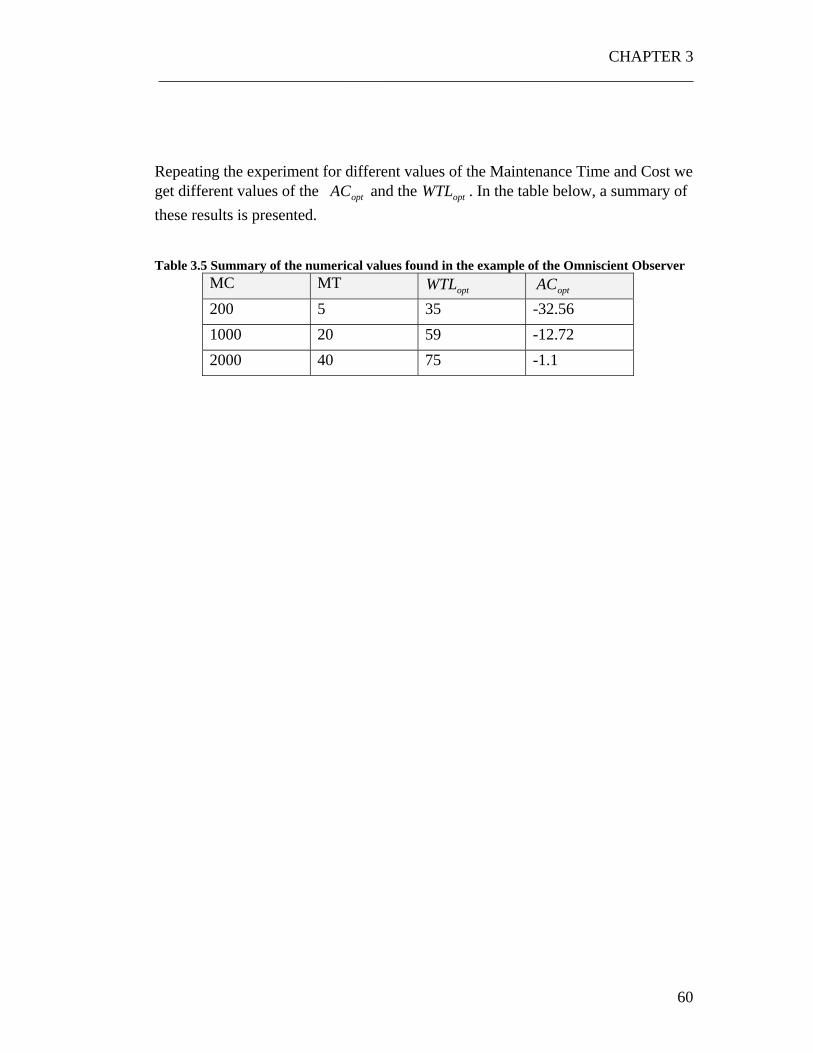
CHAPTER 3 ___________________________________________________________________
60
Repeating the experiment for different values of the Maintenance Time and Cost we get different values of the optAC and the optWTL . In the table below, a summary of these results is presented. Table 3.5 Summary of the numerical values found in the example of the Omniscient Observer
MC MT optWTL optAC 200 5 35 -32.56 1000 20 59 -12.72 2000 40 75 -1.1

Chapter 4
The Controlled System case 4 As showed in the last chapter, the Renewal Processes Theory can be successfully applied to solve a simple problem like the Periodic Maintenance Case. The purpose of that example was to provide a simple framework of how the model works and of the set of steps which lead to the final solution of the problem. However, as stated in the first chapter, the target of this work is to find an optimal control policy based on the observations of the quality of the parts. In other words, we want the controller to check and record the quality measurement of the parts every time step, and take a cost optimal decision (start maintenance or keep the system working) based on the measurements history and on the dynamic of the deterioration. Moreover, we want such measurements to be continuous and we want the controller’s decision to be based upon the whole measurement history, without scrapping any observation. What we need to do first, is to find a satisfying way to model the interaction of the controller with the system. Once we have that, we can apply the techniques learnt for the non-controlled system case and solve the problem.

CHAPTER 4 ___________________________________________________________________
62
4.1 Model of the controlled system The Markov Chain in Figure 4.1 can be a possible way to model such situation:
Figure 4.1 Markov chain of a controlled deteriorating system The probabilities )(npi that connect each working state with the maintenance state model the interaction of the controller with the system. Given that the system is working, as so given that it is in any of the working states, there is always a probability that the controller may decide to stop the system and start maintenance. In fact, the system controller bases his decisions on the parts observations, which are random variables. Such probabilities change for different states because, moving towards more deteriorated states, the likelihood that “bad” parts are manufactured, and so that the system controller may be convinced to start maintenance, increases. It may seem strange that there is a probability of transition to maintenance also for the good states, like the first one: why should the controller decide to stop the system when the it is in its best state? However, we need to remember that the quality of the parts is a random variable, and so there is always a probability that the system will generate so many “bad” parts to convince the controller that the machine is in a bad state and so to start maintenance, even if the machine is actually in a good state. The probabilities )(npi are also time dependent: the system controller is more likely to believe that the system is in a bad state if a long time has elapsed since the last maintenance, regardless of the real state where the system is. In fact, for instance, if a sequence of bad observations is recorded immediately after maintenance has been completed, the controller is likely to believe that it was just an unlucky event and that the system is in a good state. On contrary, if the same
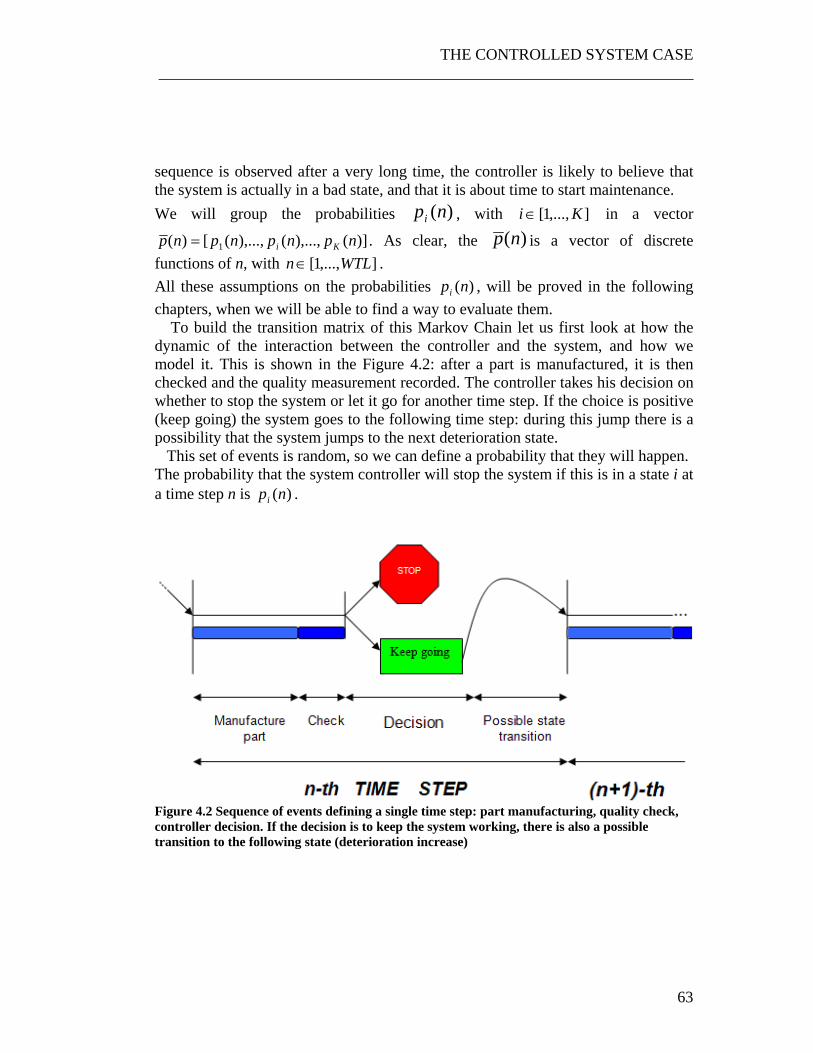
THE CONTROLLED SYSTEM CASE ___________________________________________________________________
63
sequence is observed after a very long time, the controller is likely to believe that the system is actually in a bad state, and that it is about time to start maintenance. We will group the probabilities )(npi , with ],...,1[ Ki ∈ in a vector
)](),...,(),...,([)( 1 npnpnpnp Ki= . As clear, the )(np is a vector of discrete functions of n, with ],...,1[ WTLn ∈ . All these assumptions on the probabilities )(npi , will be proved in the following chapters, when we will be able to find a way to evaluate them. To build the transition matrix of this Markov Chain let us first look at how the dynamic of the interaction between the controller and the system, and how we model it. This is shown in the Figure 4.2: after a part is manufactured, it is then checked and the quality measurement recorded. The controller takes his decision on whether to stop the system or let it go for another time step. If the choice is positive (keep going) the system goes to the following time step: during this jump there is a possibility that the system jumps to the next deterioration state. This set of events is random, so we can define a probability that they will happen. The probability that the system controller will stop the system if this is in a state i at a time step n is )(npi .
Figure 4.2 Sequence of events defining a single time step: part manufacturing, quality check, controller decision. If the decision is to keep the system working, there is also a possible transition to the following state (deterioration increase)
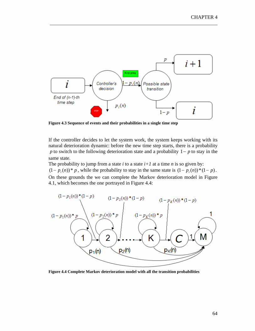
CHAPTER 4 ___________________________________________________________________
64
Figure 4.3 Sequence of events and their probabilities in a single time step If the controller decides to let the system work, the system keeps working with its natural deterioration dynamic: before the new time step starts, there is a probability p to switch to the following deterioration state and a probability p−1 to stay in the
same state. The probability to jump from a state i to a state i+1 at a time n is so given by:
pnpi *))(1( − , while the probability to stay in the same state is )1(*))(1( pnpi −− . On these grounds the we can complete the Markov deterioration model in Figure 4.1, which becomes the one portrayed in Figure 4.4:
Figure 4.4 Complete Markov deterioration model with all the transition probabilities

THE CONTROLLED SYSTEM CASE ___________________________________________________________________
65
The transition probability matrix hence becomes:
))(1)(1()( nppnpp ii −−=
⎥⎥⎥⎥⎥⎥⎥⎥
⎦
⎤
⎢⎢⎢⎢⎢⎢⎢⎢
⎣
⎡
−−
−−−−
=
1............010.........0
)()()(1)(0....................
)(...0)()(1)(0)(......0)()(1)(
)(
2222
111
npnppnpnpp
npnppnpnppnpnppnpnpp
nPKKKK
i
ART
We will call this matrix as artificial Transition Probability Matrix and indicate it as
ARTP , because it considers the natural dynamic of the system and the effect of the controller on it at the same time . If there is no control action, the probabilities )(npi become equal to zero, and the
ARTP matrix becomes identical to the natural Transition Probability Matrix P. To each control policy there will be a specific set of functions
)](),...,(),...,([)( 1 npnpnpnp Ki= associated: intuitively, the more conservative a control policy is, the higher such probabilities will be. If we had a way to calculate these functions given a generic control policy we would be able to build the ARTP matrix and so to find the Average Cost of that control policy using the algorithm in Figure 3.8. We would then iterate among different control policies and eventually find the one which optimizes the average cost. The real problem so comes down to finding a viable way to calculate the
)(np vector for a given control policy. However, before doing that, we must be able to understand which is the information that the controller uses to take his decisions and how the control policy should be structured. This is what we will do in the next three chapters.
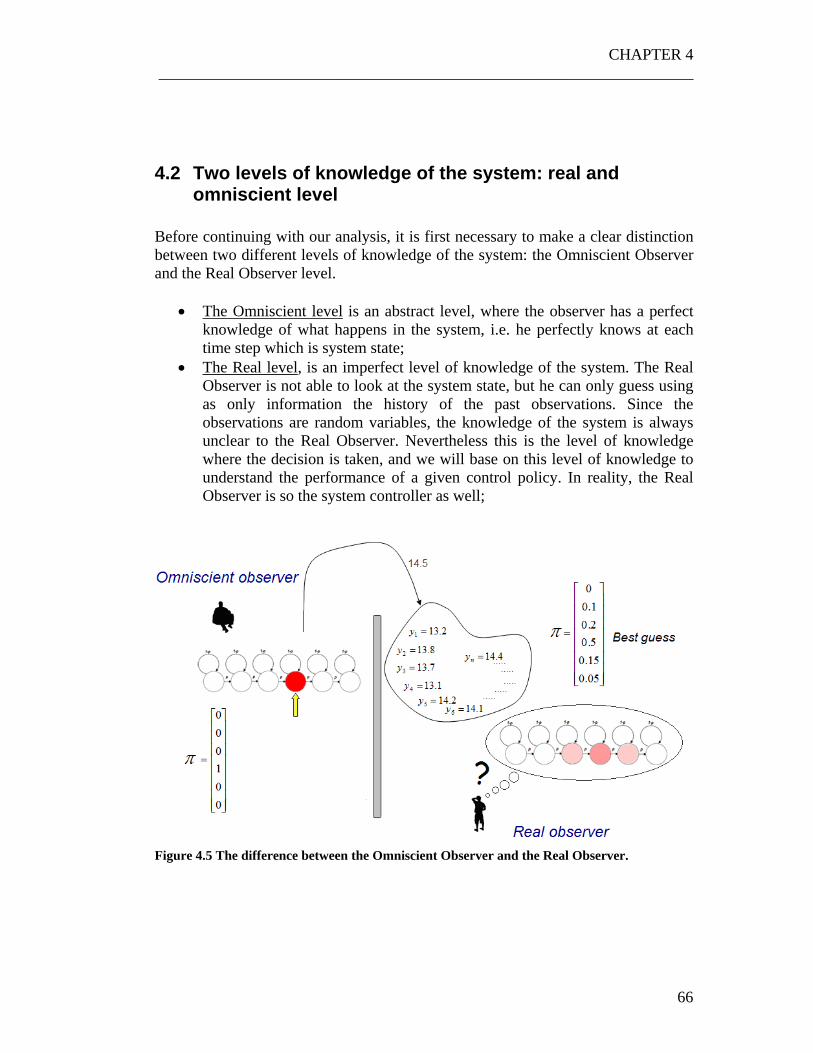
CHAPTER 4 ___________________________________________________________________
66
4.2 Two levels of knowledge of the system: real and omniscient level
Before continuing with our analysis, it is first necessary to make a clear distinction between two different levels of knowledge of the system: the Omniscient Observer and the Real Observer level.
• The Omniscient level is an abstract level, where the observer has a perfect knowledge of what happens in the system, i.e. he perfectly knows at each time step which is system state;
• The Real level, is an imperfect level of knowledge of the system. The Real Observer is not able to look at the system state, but he can only guess using as only information the history of the past observations. Since the observations are random variables, the knowledge of the system is always unclear to the Real Observer. Nevertheless this is the level of knowledge where the decision is taken, and we will base on this level of knowledge to understand the performance of a given control policy. In reality, the Real Observer is so the system controller as well;
Figure 4.5 The difference between the Omniscient Observer and the Real Observer.

THE CONTROLLED SYSTEM CASE ___________________________________________________________________
67
When the system is in a given state i, the Observer has no way to know it: he can only guess, and give a probability to each of the K working states of the system. If his way of guessing is good, and if he is not unlucky, his estimation will be reasonably close to the reality and so he will take good decisions. This information is represented by the system probability vector It is very important to keep this difference clear, because it is simple to confuse these two different levels of knowledge. When we will talk about the system itself, i.e. the true state where the system is, we will talk from an Omniscient level point of view. But when we refer to the controller decisions, we always have to think from an Real Observer point of view, i.e. from an imperfect and approximated vision of the real system.

CHAPTER 4 ___________________________________________________________________
68
4.3 Research of the optimal control policy for an Omniscient controller
The Real Observer is who, in the real system, takes the action of stopping the system and starting maintenance. The Observer’s decisions are always worse then those of an hypothetical Omniscient observer. Given a system, every real control policy can be improved but there is a maximum virtual limit given by the optimal control policy for an Omniscient observer. If we found the Average Cost of a system controlled by an Omniscient controller we would automatically get the ‘natural’ limit of that system: it is impossible to further improve that Average Cost (unless we changed the system itself). On these grounds finding that limit and finding that control policy could be used as a benchmark, and it is what will developed in this subsection. The interaction of an Omniscient controller with the system can still be modeled with the Figure 4.4. In this case though, the )(npi can be either 0 or 1: since the controller knows at each time what is the real state of the system, there is no uncertainty and he can take deterministic actions. Searching the optimal control policy in this case is simple: we have to understand which states of the system are ‘good’ and which ones are ‘bad’. In other words we have to tell the controller “stop the system when it gets in the i-th state”; the point is to find the i which optimizes the Average Cost of the system. If we stop it in one of the early states, we avoid to produce ‘bad’ parts, thus guaranteeing high revenues from the manufactured products. However, we spend a significant part of each Maintenance Cycle performing maintenance. On contrary, if we stop the system in one of the last states, we get long Working Times (because we start maintenance only when it is truly necessary) but we are likely to manufacture a lot of ‘bad’ parts. This is a not trivial trade-off, especially because we do not manufacture only ‘good’ or ‘bad’ parts, but parts with real quality measurement y, to which a specific cost )(yς is associated. Moreover the trade off strongly depends on how long and how expensive maintenance is (if maintenance is long and expensive, the controller is likely to start maintenance as late as possible). This problem can be easily solved using the RPT approach. Let us take the scheme in Figure 3.7 and let us modify it a little: the structure of the problem is pretty much the same; what changes is the P matrix and the fact that we do not need to impose a WTL since it would be senseless to mix a Periodic Maintenance with a controlled maintenance.

THE CONTROLLED SYSTEM CASE ___________________________________________________________________
69
Now a controller policy for the an Omniscient observer is a limit α such that: When i=α stop the system. If i<α keep the system working with ℵ∈α and K≤≤ α1 . The target is to find the OPTα such that the Average Cost is minimum. Like usually, we will find an iterative approach to solve the problem. To each α there is an associated vector )(np containing the probabilities of transition from a working state to the maintenance state.
⎥⎥⎥⎥
⎦
⎤
⎢⎢⎢⎢
⎣
⎡
==
Kp
pp
pnp...
)( 2
1
Where in this case ip is either 1 or 0. We will thus have that, for example:
K=α
⎥⎥⎥⎥⎥⎥
⎦
⎤
⎢⎢⎢⎢⎢⎢
⎣
⎡
=
00...00
p 1−= Kα
⎥⎥⎥⎥⎥⎥
⎦
⎤
⎢⎢⎢⎢⎢⎢
⎣
⎡
=
10...00
p
2=α
⎥⎥⎥⎥⎥⎥
⎦
⎤
⎢⎢⎢⎢⎢⎢
⎣
⎡
=
1...100
p 1=α
⎥⎥⎥⎥⎥⎥
⎦
⎤
⎢⎢⎢⎢⎢⎢
⎣
⎡
=
11...10
p
It is now possible to build an iterative algorithm like the one shown in Figure 4.6 where the value of α is gradually changed and the Average Cost is calculated.

CHAPTER 4 ___________________________________________________________________
70
Figure 4.6 Iterative algorithm for the research of the cost optimal policy for an Omniscient observer. The value of WTL in this case should be hypothetically equal to infinite (there is no policy constraint on the duration of a maintenance cycle) but for computational purposes it should be limited to a reasonable ‘large enough’ value.

THE CONTROLLED SYSTEM CASE ___________________________________________________________________
71
As an example, we will solve the same problem we had solved for the Periodic Maintenance case in Section 3.3.4, using this time an Omniscient Observer controller. The Probability Density Functions of the quality of the parts of the controlled system are always the same as well as the cost function (please see Figure 3.9 and Figure 3.10). We will then apply the algorithm in Figure 4.6 to find the cost optimal policy. The Figure 4.7 shows an example of the Markov Chain of the deteriorating machine used in the Periodic Maintenance example, controlled by an Omniscient observer.
Figure 4.7 Markov Chain of a deteriorating system controlled by an omniscient observer. The
control policy in this case is for alfa=3 We have solved the same problem, using the same values of Maintenance Time and Maintenance Cost we had used for the Periodic Maintenance case. The Figure 4.8, Figure 4.9 and Figure 4.10 show how the Average Cost changes as the control policy changes.

CHAPTER 4 ___________________________________________________________________
72
MC=1000; MT=20
-30
-20
-10
0
10
20
30
40
50
1 2 3 4
Alfa
Ave
rage
Cos
t
Figure 4.8 Average Cost of different control policies, for a system with a Maintenance Cost=1000 and a Maintenance Time=20.
MC=200; MT=5
-50
-40
-30
-20
-10
0
10
20
30
1 2 3 4
Alfa
Ave
rage
Cos
t
Figure 4.9 Average Cost of different control policies, for a system with a Maintenance Cost=1000 and a Maintenance Time=20.

THE CONTROLLED SYSTEM CASE ___________________________________________________________________
73
MC=2000; MT=40
-20
-10
0
10
20
30
40
50
60
1 2 3 4
Alfa
Ave
rage
Cos
t
Figure 4.10 Same experiment for a MC=2000 and a MT=40 It is interesting to notice that as the maintenance burden increases (MC and MT increase) the optimal control policy moves to higher values of α . This means that the cost for performing maintenance is higher then the additional cost for manufacturing bad or ‘poor quality’ parts. A comparison between the Average Cost of the system using a Periodic Maintenance or an Omniscient observer policy is presented in Table 4.1 Table 4.1 Comparison between the optimal Average Costs of the same system using a Periodic and an Omniscient observer policy
MC MT optAC Periodic optAC Omniscient % ACΔ 200 5 -32.56 -41.34 -27% 1000 20 -12.72 -25.14 -97% 2000 40 -1.1 -13.11 -1092%
CHAPTER 4 ___________________________________________________________________
74
As clear, there is a sharp difference in the Average Cost of the system between using a Periodic and an Omniscient observer policy. Such difference increases exponentially as the maintenance burden increases: in these situations the choice of starting maintenance becomes more and more important and so a more sophisticated method for taking such decision is compensated by a significantly higher performance. The control policies we will be looking for in the next chapters are different from the Omniscient observer control policy that has just been analyzed. The Real observer, in fact, does not know what is the true state of the system, but he has an idea of what is the probability that the system is in any of the working states. Therefore, we must expect the optimal Average Cost to be higher then the one of an Omniscient observer. However, as underlined in the Table 4.1, there is a huge margin between the Periodic maintenance and the Omniscient observer maintenance, so there is still a lot that we can do to improve the performance of the system.

THE CONTROLLED SYSTEM CASE ___________________________________________________________________
75
4.4 The a priori and the a posteriori system probability vectors
As a first step to take cost optimal decisions it is necessary to understand what is the information that the Real observer has about the system and how he builds such information. As explained in Chapter 4.2, the difference between an Omniscient observer and a Real observer is that while the former knows exactly which is the system state at each time step, the latter is able to create a probability to be in each state. In other words he can base his decision on a probability vector π , that we called system probability vector, containing the value of all the probabilities of being in any of the working states. The controller knows that, after maintenance, the system restarts from the first state with probability 1. This is the only time step where he knows the system state exactly:
]0..01[0 =π ( 4.1)
In all the time steps other than the first one, the controller does not know the state of the system deterministically, but he can only assign a probability to each state. There are two sources of randomness generating this lack of knowledge: the probability density function of the quality of the parts and the Markov chain deterioration dynamic of the system. For what said at the beginning of this document, we want the observer to base his decision on all the information gathered since the beginning of the maintenance cycle, without scrapping anything. This means that the observer’s knowledge about the system should be based on the whole history of the observations and the observations he records should be continuous. Moreover, such information is also completed by the knowledge of the deterioration dynamic of the system, in our case the Markov deterioration model. This way, we will be able to find the best estimation of the system state and we will thus be able to take the best possible action. At each time step the machine produces a part with a quality measurement y. We will use a subscript to associate each observation to the time step when it has been manufactured: for example the observation of the time step 3 will be called 3y . Each generic ny is a real numeric value, in other words the true value that has been measured at n-th time step. We will instead use the notation )(ny to refer to the value that has been recorded and stored in memory at each time step. In other words
CHAPTER 4 ___________________________________________________________________
76
)(ny can be see as the empty memory slot to store the numerical value ny of the observation that will measured at the time step n. At the time step n the controller has thus recorded n observations which are stored in an observation vector })1(...,,)({ 1yyyny nn ===Ψ . We want to find the conditional probability of being in the generic i-th, given the observation vector nΨ . If we denote the state of the system at the time step n as
)(ns we can write this conditional probability as:
)|)(())1(,....,)(|)(( 1 nn insPyyynyinsP Ψ===== ( 4.2)
Please note that, as desired, in finding this probability we are using the whole observations history, and all the observations are continuous. For the Bayes theorem:
)|)(()|)(,)((
))1(,....,)1(|)(())1(,....,)1(|)(,)((
)|)((
1
1
11
11
−
−
−
−
Ψ=Ψ==
=
===−=
==−===Ψ=
nn
nn
nn
nnn
ynyPynyinsP
yyynyynyPyyynyynyinsP
insP
(4.3)
And so, still using the Bayes theorem and exploiting the conditional independence of )}({ ny and }{ 1−Ψn when })({ ins = , we get:
=Ψ=
Ψ=Ψ===
Ψ=Ψ==
−
−−
−
−
)|)(()|)(() ,)(|)((
)|)(()|)(,)((
1
11
1
1
nn
nnn
nn
nn
ynyPinsPinsynyP
ynyPynyinsP
)|)(()|)(() )(|)((
1
1
−
−
Ψ=Ψ===
=nn
nn
ynyPinsPinsynyP
(4.4)
THE CONTROLLED SYSTEM CASE ___________________________________________________________________
77
Now consider:
)|)1(( ),)1(|)((
)|)1(,)(()|)((
11
11
−−
−−
Ψ=−Ψ=−==
=Ψ=−==Ψ=
∑
∑
nj
n
nj
n
jnsPjnsinsP
jnsinsPinsP
( 4.5)
where r is another generic state ],...,1[ Kj ∈ . But from the conditional independence of })({ ins = and }{ 1−Ψn when })1({ jns =− we have that:
jin PjnsinsPjnsinsP ==−==Ψ=−= − ))1(|)((),)1(|)(( 1
( 4.6 )
Where jiP is the transition probability from the state i to the state j, i.e. the element ji of the transition probability matrix P. We therefore have:
)|)((
)|)1(( ))(|)(()|)((
1
1
−
−
Ψ=
Ψ=−===Ψ=
∑nn
jnjin
n ynyP
jnsPPinsynyPinsP
( 4.7 )
We can repeat the same procedure for the denominator. If we notice that, for ],...,1[ Kk ∈
∑ −− Ψ===Ψ=k
nnnn knsynyPynyP )|)(,)(()|)(( 11 ( 4.8 )
We get the same thing we had started from in the Equation (4.3) Thus, the Equation ( 4.7) can be rewritten as:
∑ ∑∑
−
−
Ψ=−==
Ψ=−===Ψ=
k jnjin
jnjin
n jnsPPinsynyP
jnsPPinsynyPinsP
)|)1(( ))(|)((
)|)1(( ))(|)(()|)((
1
1
( 4.9 )
For the problem we are studying we have that:
CHAPTER 4 ___________________________________________________________________
78
))(|)(( insynyP n == = nni dyyf ) (
( 4.10 )
where )(yfi is like usually the Probability Density Function of the quality of the parts for the state i. So, finally:
∑ ∑∑
−
−
Ψ=−
Ψ=−=Ψ=
k jnjknk
jnjini
n jnsPPyf
jnsPPyfinsP
)|)1(( )(
)|)1(( )()|)((
1
1
( 4.11 )
We can now introduce an important concept. If we consider that }{ nΨ can also be rewritten as },)({ 1−Ψ= nnyny , then we have that ),)(|)(()|)(( 1−Ψ===Ψ= nnn ynyinsPinsP . This gives us a new vision of the problem: this is the probability that the system is in the state i at the time n [ ins =)( ], given an observations history 1−Ψn and given that a new observation nyny =)( has just been recorded. We will call this quantity as the a posteriori probability of being in the state i at the time n, i.e. the probability of being in the state i at the state n immediately after (a posteriori) a new observation has been measured. This variable will be called with the symbol )(in
+π , i.e.:
),)(|)(()|)(()( 1−+ Ψ===Ψ== nnni ynyinsPinsPnπ
( 4.12 )
The Equation ( 4.11 ) hence becomes:
∑ ∑∑
+−
+−
+ =
k jnjknk
jnjini
i jPyf
jPyfn
)( ) (
)( ) ()(
1
1
π
ππ
( 4.13 )
If we do this same calculation for all the ],...,1[ Ki ∈ we can build a vector,
)](),...,(),...,1([ Ki nnnn++++ = ππππ
( 4.14 )
THE CONTROLLED SYSTEM CASE ___________________________________________________________________
79
that we will call a posteriori system state probability vector. Since ijP is the ij element of the matrix P, we can simplify the notation considering that:
jnj
nji PjP ][)( 11 ⋅= +−
+−∑ ππ
( 4.15 )
We can thus rewrite the Equation (3.25) as:
∑ ⋅⋅
=−
−+
kknnk
innin Pyf
Pyfi
]) [(]) [(
)(1
1
ππ
π ( 4.16 )
The product Pn *1
+−π is what is usually called the a priori probability vector and is
usually indicated as −nπ .
Pnn ⋅= +−
−1ππ
( 4.17 )
The difference between the a priori and the a posteriori probability vectors is that while the first finds an estimation of the system state at a time n before watching the new manufactured part, the second uses such information to update the system state. In other words while the )(n+Π includes the most recent information to evaluate the systems state, the )(n−Π uses the information of the previous time step and exploits the system dynamic (through the P matrix) to figure out what is the system state at the time n. The Equation ( 4.16 ) can thus be re-written as:
∑ −
−+ =
kknnk
innin yf
yfi]) [(
]) [()(π
ππ
( 4.18)
We can so summarize how the system controller updates his knowledge of the system state in the following way:
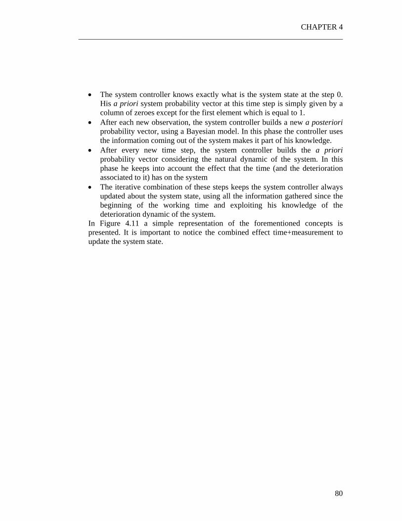
CHAPTER 4 ___________________________________________________________________
80
• The system controller knows exactly what is the system state at the step 0.
His a priori system probability vector at this time step is simply given by a column of zeroes except for the first element which is equal to 1.
• After each new observation, the system controller builds a new a posteriori probability vector, using a Bayesian model. In this phase the controller uses the information coming out of the system makes it part of his knowledge.
• After every new time step, the system controller builds the a priori probability vector considering the natural dynamic of the system. In this phase he keeps into account the effect that the time (and the deterioration associated to it) has on the system
• The iterative combination of these steps keeps the system controller always updated about the system state, using all the information gathered since the beginning of the working time and exploiting his knowledge of the deterioration dynamic of the system.
In Figure 4.11 a simple representation of the forementioned concepts is presented. It is important to notice the combined effect time+measurement to update the system state.
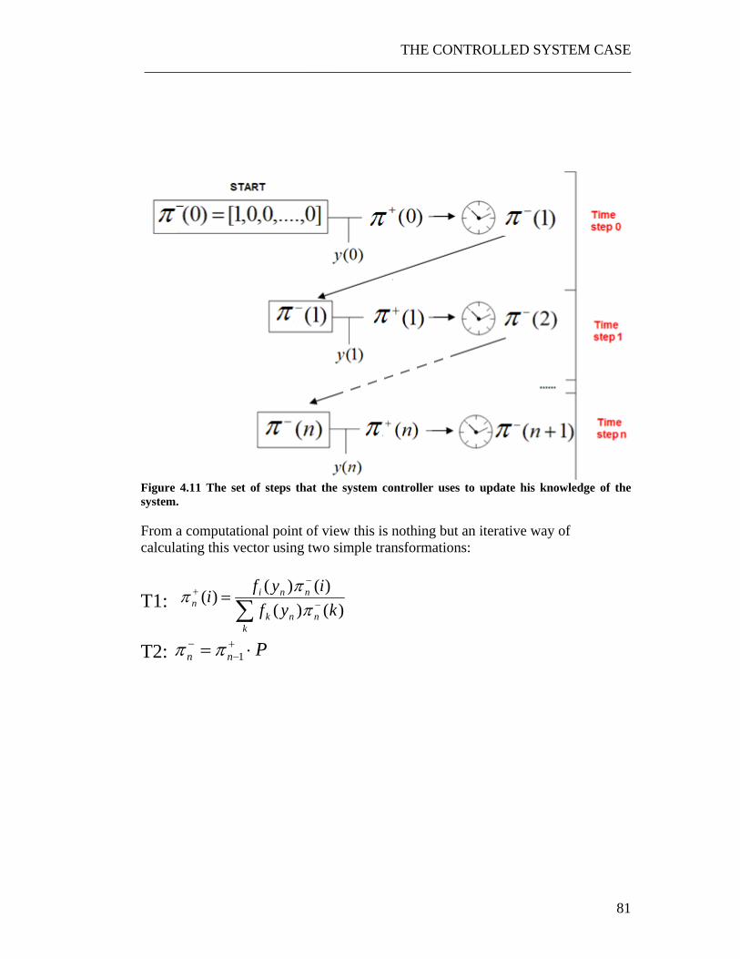
THE CONTROLLED SYSTEM CASE ___________________________________________________________________
81
Figure 4.11 The set of steps that the system controller uses to update his knowledge of the system. From a computational point of view this is nothing but an iterative way of calculating this vector using two simple transformations:
T1: ∑ −
−+ =
knnk
nnin kyf
iyfi)() (
)() ()(π
ππ
T2: Pnn ⋅= +−
−1ππ
CHAPTER 4 ___________________________________________________________________
82
Figure 4.12 Algorithm for the computation and updating the system state vector

THE CONTROLLED SYSTEM CASE ___________________________________________________________________
83
4.5 Structure and properties of the optimal control policy As shown in the previous section, the knowledge that the controller has about the system is concentrated in the +π vector. We will now prove that an optimal control policy based on this vector can be created and that such control policy has a fairly simple structure. Similar results have been proved for similar problems in other papers like Smallwood[19] and Sondik[20].
4.5.1 Time-independency of the optimal control policy: a formal explanation.
The Optimal Control Policy is a function of the posterior probability vector, but not of the time. The Optimal Control Policy function is thus stationary. There are different ways to prove this property of the control policy function, the most intuitive of which is that since the posterior probability vector Π+ is updated after every time step starting from the first one, the information about the time is naturally contained in it. Nevertheless better and more formal explanations can be found. The most convincing and rigorous of such explanations can be found starting from the results of a past publication, to which we will make explicit reference throughout this document. The publication is Fernandéz-Gaucherand [35]. We will refer to the Theorems, Lemmas and Definitions of such paper and, for helping the reader, we will write the page of the paper where they can be found (written between brackets). In this document sufficient conditions are derived for solutions to the average cost optimality equation to exist; these solutions are proved to be stationary non-randomized control policies. What is very interesting is that one of the main conditions is the presence of ‘reset actions’ i.e. of a possible controller’s action which resets the state of the system to a given deterministic state. This condition can be perfectly found in our problem, where the reset action is the maintenance. Before continuing it is important to make clear the set of conventions and symbols that we use, and above all, the way we look at the system, and compare it with the conventions used by the authors of the paper. In our model we use the Renewal Processes Theory (RPT), which helps us to find the Average Cost of the system studying it during a single maintenance cycle.
CHAPTER 4 ___________________________________________________________________
84
In order to use a common language with the authors of the paper, we will ‘forget’ in this document that the system can be simplified using the RPT2, and we will study his characteristics watching it as a generic POMDP3, with the target to optimize its Average Cost over an infinite time horizon. Watching at the system in these two different ways is absolutely identical: if we use the RPT we get the advantage to study it in a much simpler way, but nothing happens if we look at it using its ‘original’ structure. In other words, if we can safely say that for the original POMDP problem there is an Optimal Stationary Control Policy for the infinite time horizon, then does not matter how we search this policy (RPT, Dynamic Programming, etc): what we can be sure of is that the structure of this control policy is stationary. This is why, in the next pages, we won’t use the usual Markov Chain referred to a single maintenance cycle as we did in the last documents, but we will see the problem of deterioration and maintenance as a normal POMDP problem. The philosophy of this Document can be summarized in three steps :
1) Looking at the Original System, as a generic POMDP, i.e. in the same way the authors of the paper would do it.
2) Using the results of the paper to prove that for the Original System, an Optimal Control Policy exists that optimizes the Average Cost over the Infinite Time Horizon, and this policy is stationary.
3) Coming back to our model (the RPT model) to find the best control policy, but being sure that the optimal control policy we need to look for is stationary. This would imply a significant simplification, since the set of the control policies we need to explore to find the ‘best’ one would be less complex.
Like all the POMPDs we have a set of states (in our case a limited set of states), a set of actions that can be taken by the system controller (in our case 2 actions: keep the system working or start maintenance) to each of which a different Transition Probability Matrix is associated.
2 Renewal Processes Theory 3 Partially Observable Markov Decision Process

THE CONTROLLED SYSTEM CASE ___________________________________________________________________
85
Figure 4.13 Markov Chains associated to the two possible action of the controller: start
maintenance or let the system work

CHAPTER 4 ___________________________________________________________________
86
The two TPMs are thus the following:
⎥⎥⎥⎥⎥⎥
⎦
⎤
⎢⎢⎢⎢⎢⎢
⎣
⎡
−−
−−
=
MTTRMTTRpp
pppp
P
11......110....
..........0..100..01
)1(
⎥⎥⎥⎥⎥⎥
⎦
⎤
⎢⎢⎢⎢⎢⎢
⎣
⎡
−
=
MTTRMTTR
P
11......11..................1........1....00
)2(
The fact that the last row is the same for both the TPM shows that no action can be taken by the controller when the system is in the Maintenance state (he simply has to wait for Maintenance to be completed). Given a state where the ‘core’ system is, there is a cost associated to each action
),( uiC . Since we have two only possible actions we will have two of these vectors.
⎥⎥⎥⎥⎥⎥⎥⎥
⎦
⎤
⎢⎢⎢⎢⎢⎢⎢⎢
⎣
⎡
+
= ∫
∫
∈
∈
0
)()(...
)()(
)(:,
1
1
MCCC
dyyfyC
dyyfyC
uCYy
K
Yy
and
⎥⎥⎥⎥⎥⎥
⎦
⎤
⎢⎢⎢⎢⎢⎢
⎣
⎡
=
0
...)(:, 2
MCMC
MC
uC
Where C(y) is the usual cost function, )(yf K is the Probability Density Function of the generic state K, CrashC is the Crash Cost and MC is the Maintenance Cost. If the controller let the system work (u1) in any of the K states we have the usual expected cost associated to every state (and given by the integral of the C(y) over f(y)) , while if it let it work when it is in the Crash State the system has to pay the cost of maintenance plus the extra Crash Cost.
THE CONTROLLED SYSTEM CASE ___________________________________________________________________
87
If the controller decides to stop the system (u2), the only cost that he has to pay is the Maintenance Cost. Once the system is in the Maintenance State, there is no cost to pay, and no action is possible (the system has already paid the cost for maintenance and simply waits until this is completed). An important assumption of the paper is that all costs are positive. This means that, if there are states for which there is a revenue (a negative cost) we need to add a constant in order to make them all positive. As obvious, and stated by the authors of the paper, this does not change the results. The first thing that could be objected is that in this way we only consider exponentially distributed repair times and constant maintenance costs, while in our original model (the RPT model) we manage to deal with any type of probability distribution of these two variables. As shown in Appendix I of this document, the Average Cost (over an infinite time horizon) for our problem depends only on the Expected Values of these two variables and not on their probability distributions. So, however we model them, their effect on the Average Cost depends only on their Expected Values. The expected time to repair is called MTTR. Given an a priori state probability vector, the expected one step cost is so given by:
)(:;*),( uCuc −− =Π π , which means that (as obvious) if the choice of the system is u2 the one step cost is constant, independent of the a priori and equal to MC. The reason why in our RPT model we do not consider the Crash and the Maintenance state in the control policy function is because both the Crash and the Maintenance state are perfectly observable states (i.e. if the real system is either in the Crash or in the Maintenance state, the a posteriori system state probability vector would be a column of zeros except for the C or M state where there would be a 1). The same thing is not true for the a priori probability vector. We are not sure that the system is in the Crash state if we have not ‘observed’ it yet. On contrary, if we can see the next observation and notice that instead of producing a part the system ‘fails’ we know with probability 1 that the system is in the Crash state. This is why in the a posteriori system state probability vector, both the Crash and the Maintenance state are deterministic. In our model we have decided to express the Control Policy as a function of the a posteriori and not of the a priori vector because it gives us the advantage that, since no action can be taken by the system controller after it observes that the system is in either the C or the M state (i.e. when it has already and clearly observed that the system has failed or that it has been sent to maintenance) , there is no need to use such states in the control policy function. Using the a priori or the a posteriori probability vector is absolutely the same in our case, because these two vectors are bounded by a linear correlation:

CHAPTER 4 ___________________________________________________________________
88
Pnn *1+−
− = ππ ; the only difference is that in the first case we would have a more complex model because we should also consider the Crash state. This means that if (in our case) we discover that the an Optimal Stationary Control Policy, function of the a priori state probability vector exists, then the same thing must happen for a Control Policy expressed as a function of the a posteriori vector. This is important to say because the authors of the paper, dealing with a general situation, use all the states of the system and express the control policy as a function of the a priori vector. For what stated before, studying our system using these conventions instead of ours would imply no modification to the real structure of the problem. Before continuing, we also need to “translate” the language used in the paper with our language. The concepts and the used variables are always the same, but called with different names. In the following schedule I have tried to summarize the set of the used variables: (For those variable that do not have a name in our model, we will henceforth use the same notation of the Paper. These variables are indicated with a superscript * ). Original
Paper This
document Meaning
X X* Set of all the states of the “core” Markov Chain Nx Κ+2 Number of states of the “core” Markov Chain. In our case it
is given by K plus the C and the M state. p
−π A priori state probability vector u u* System controller action y y Observation
T(y,p,u) π+ A posteriori state probability vector. Even though we do not make it explicit in the notation of our original notation, Π+
is a function of y, Π- ,and u in our model as well. Δ Δ Set of all the possible values of the Π- vector. This is
similar to the hyperpyramid (we used to call HYP), but it is in the space RK+2 because it has to include the Crash and the Maintenance states.
U U* Set of al the possible actions of the controller. In our model this set is composed by two only elements: u1 (keep the system working) and u2 (stop the system and start maintenance).
Y Υ Set of all the possible observations μ(..) f(..) Control Policy Function
THE CONTROLLED SYSTEM CASE ___________________________________________________________________
89
In order to make the Document more easily to read I have translated the notation used in the paper with our usual one. The only thing that I needed to change is the posterior probability vector, making explicit that it is a function of the observation y, the controller decision u and the a priori system probability vector −Π .
),,( 1 uy −++ ⇒ πππ Summarizing the fundamental concepts, the paper states through the Theorem 4.2 (Pag.19) that, If 2 fundamental conditions are satisfied (generically called condition (C) and (UBGT)), then there is a solution to the Average Cost Optimality Equation; any (non-randomized) stationary separated policy attaining the minimum in such equation is average cost optimal and moreover one such policy exists. For non-randomized separated policies, the authors indicate a sequence of measurable maps Ut →Δ:μ , i.e. a sequence of system controller actions (defined in the set of the possible actions U, in our case a two elements set) depending on the set Δ , which in our case is the hypepyramid HYP. The control policy is stationary if μμ =t for all the values of t. (Pag. 7). If such conditions are verified, we are sure that an optimal stationary control policy that minimizes the Average Cost exists, and so, in our search for the ‘best’ control policy, we are justified to explore only stationary policies (thus seriously reducing the complexity of the problem). In the following pages we will show that these two conditions apply for our problem. Condition 1 (C) (Pag.13) For all Υ∈y , Uu ∈ , and Δ∈−π , [ ] 1),,( −−+ Π uyπ is a countable set. Where [ ] 1),,( −−+ Π uyπ is the inverse of the function ),,( uy −+ ππ . This condition is then relaxed, and a new condition (C)’ is formulated, which is perfectly equivalent to the first one Condition 1 (C)’ (Pag.20) Perfectly equivalent to the condition (C)
CHAPTER 4 ___________________________________________________________________
90
The action set U can be partitioned as 21 UUU ∪= such that:
(i) [ ] 1),,( −−+ uy ππ is a countable set, for all Yy ∈ , 1Uu ∈ and Δ∈−π (ii) The set { }2,,|),,( Uuyuy ∈Δ∈Ξ∈ −−+ πππ is finite It is possible to show that both of these conditions are actually satisfied in our case. Our set U is given by two only elements: let’s call U1 the one element set containing the choice to keep the system working, and U2 the one element set containing the choice to start maintenance. It is immediately possible to state that condition (ii) is satisfied since, when we decide to start maintenance (so when 22 Uuu ∈= ) the system can only be in the maintenance state with probability one in the following time step. This mean that the set { }2,,|),,( Uuyuy ∈Δ∈Υ∈ −−+ πππ is a one element set (and thus finite) with +Π being a column of zeros except for the Maintenance state where it is a 1. To satisfy the condition (i), the authors notice (Pag.14 Remark 4.1), that it is sufficient that ),,( 1 uy −+ ππ is an injective map, for any 1, Uuy ∈Υ∈ . It is then proved (Pag.14 Lemma 4.2) that if we suppose that both X (the set of the states of the ‘core’ system) and Y (the set of all the possible observations y) are countable sets, two sufficient conditions for ),,( 1 uy −+ ππ to be an injective map is that the 2 matrices { })(:)( 1,1 uqdiaguQ yiy = (Pag.6) and )( 1uP (the transition probability matrix associated to the choice 1u ) are both non singular. Let us prove these conditions for our case. About the statement that X is a finite set we have no doubt since the number of states through which the machine deteriorates is finite. We could not say the same thing about Y, because we deal with continuous measurements; but if we look at the real problem we can infer that Y is actually countable. Y, in fact, is the set of the observations y(n) that the controller has about the parts leaving the machine. Every measurement is performed by an instrument of measurement, and every instrument of measurement or sensor has a given resolution (i.e. the smallest change it can detect in the quantity that it is measuring). This means that, even though the sensor has a very precise resolution, the measurements are always discretizable (where the discretization is given by its resolution), and so the set of all the possible measurements Y is consequently countable. The advantage of our model (RPT approach) is that we can arbitrarily increase the discretization (making it equal to the true discretization performed by the
THE CONTROLLED SYSTEM CASE ___________________________________________________________________
91
instrument of measurement) without incurring any computational difference in comparison with a poor discretization. Now that we know that both Y and X are countable sets we still need to check that the matrices { })(:)( 1,1 uqdiaguQ yiy = and )( 1uP are non singular. The matrix { })(:)( 1,1 uqdiaguQ yiy = (Pag.6) with
))(,)1(|)1(()( 11, unuinsynyPuq yi ==+=+= (Pag.4).
In other words there is a matrix yQ for every observation y, which is a diagonal matrix with the values of the probabilities that, if an observation y is recorded, the system state is i. These probabilities, as we know, are given by the Probability Density Function associated to every state. If the discretization is sufficiently dense, they can be written as dyxf ni ) ( 4, where f is the PDF5 and dy is the order of discretization (instrument resolution) If the discretization is not dense enough, they are simply the integral of the PDF between the two boundaries of the discretization interval. Since the yQ are diagonal matrices, the only thing to guarantee that their 0det ≠ and so that they are invertible, is that no element of the diagonal is equal to 0. To get this condition we need that all the PDF of all the states should never be equal to 0. This condition is quite easy to be satisfied, since in the most used PDF (Gaussian, etc) to describe the quality of parts )(yf is never equal to 0. In other words we should never use PDFs that are ‘truncated’ in the range of values of y for which Υ∈y . As regards the )( 1uP matrix (please, look at the page 3 of this document) it is quite easy to notice that this is never a singular matrix (for every value of p) since none of its rows is linearly correlated to the others. Since we checked that all the conditions to prove the points (i) and (ii) of the Condition 1 are verified, we can say that the Condition 1 (C)’ is satisfied. Condition 2 (UBGT) (pag.16) As said at (Pag.16) this condition is satisfied if another condition (UB) is satisfied.
4 Please, see the document “The properties of the control policy function. Part1” at pag.2 5 Probability Density Function

CHAPTER 4 ___________________________________________________________________
92
The condition (UBGT) is less strict then (UB) since it requires an inequality to be satisfied in a define subset GT of Δ. For our problem we can prove that such inequality is verified Δ∈∀ −π , thus satisfying the stronger (UB) condition. To prove this condition we will have to introduce some definitions. Let us define the discounted cost6:
⎭⎬⎫
⎩⎨⎧
Γ+=Γ ∑∈
−+−−
∈
−
YyUuuyuyVuc )),,(((),,(),(min)( πππβππ ββ
Where V(..) is the one step ahead conditional probability of the observation y given an a priori distribution of the core state and β is the discount factor.
βΓ is the expected best discounted cost if the a priori vector of the system is Π−. The condition (UB) is satisfied if (Pag.12): There is a constant M>0 such that:
Mh ≤=Γ−Γ −−− )()()( .πππ βββ , 01 <<∀ β , Δ∈∀ −π ,
Δ∈−π If there is a Δ∈−π which satisfies this inequality, then condition (UB) and so (UBGT) hold. We will show that such condition is satisfied in our case for a [ ]1..00=−π , i.e. when the a priori probability vector is in the maintenance state with probability 1 . For simplicity we will call:
[ ] −− == Mππ 1..00 The paper says that two sufficient conditions are necessary for this to be satisfied:
6 Many existing publications deal with POMDPs using a Discounted Cost approach
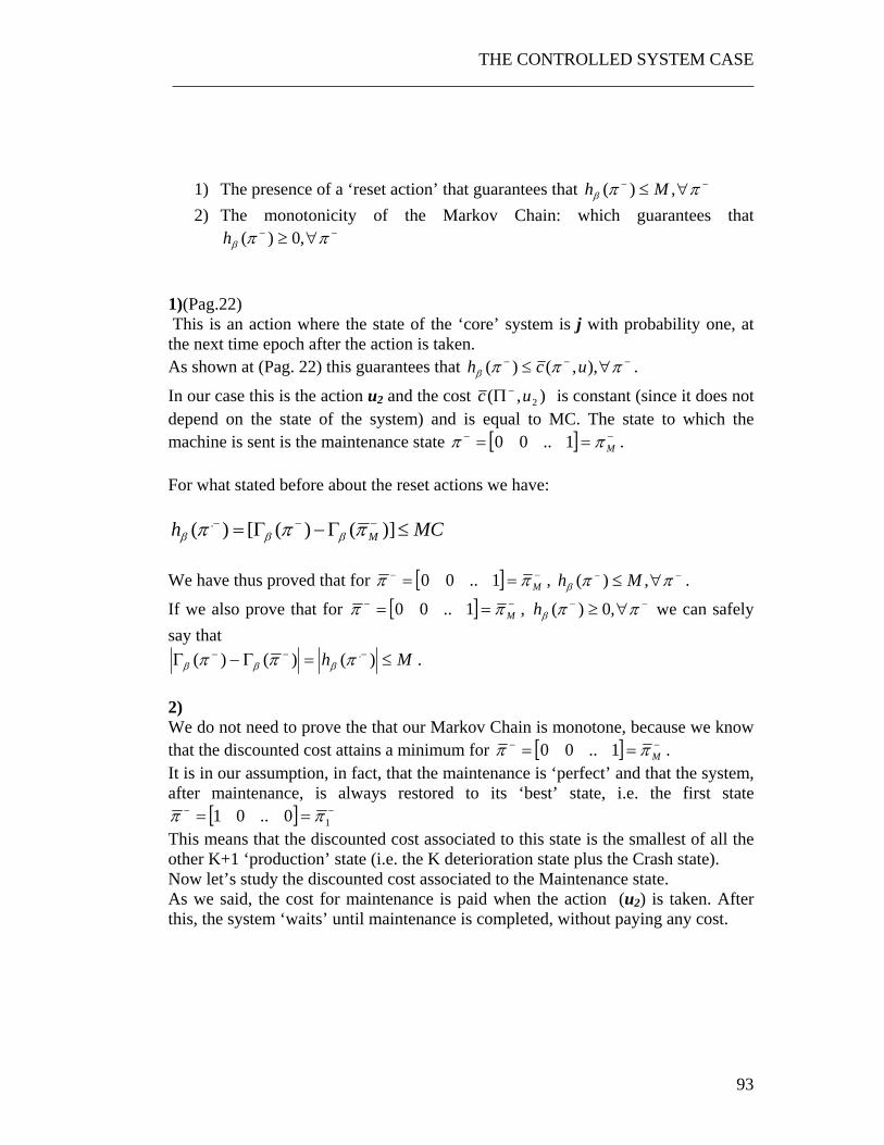
THE CONTROLLED SYSTEM CASE ___________________________________________________________________
93
1) The presence of a ‘reset action’ that guarantees that −− ∀≤ ππβ ,)( Mh 2) The monotonicity of the Markov Chain: which guarantees that
−− ∀≥ ππβ ,0)(h 1)(Pag.22) This is an action where the state of the ‘core’ system is j with probability one, at the next time epoch after the action is taken. As shown at (Pag. 22) this guarantees that −−− ∀≤ πππβ ),,()( uch .
In our case this is the action u2 and the cost ),( 2uc −Π is constant (since it does not depend on the state of the system) and is equal to MC. The state to which the machine is sent is the maintenance state [ ] −− == Mππ 1..00 . For what stated before about the reset actions we have:
MCh M ≤Γ−Γ= −−− )]()([)( . πππ βββ We have thus proved that for [ ] −− == Mππ 1..00 , −− ∀≤ ππβ ,)( Mh .
If we also prove that for [ ] −− == Mππ 1..00 , −− ∀≥ ππβ ,0)(h we can safely say that
Mh ≤=Γ−Γ −−− )()()( .πππ βββ . 2) We do not need to prove the that our Markov Chain is monotone, because we know that the discounted cost attains a minimum for [ ] −− == Mππ 1..00 . It is in our assumption, in fact, that the maintenance is ‘perfect’ and that the system, after maintenance, is always restored to its ‘best’ state, i.e. the first state
[ ] −− == 10..01 ππ This means that the discounted cost associated to this state is the smallest of all the other K+1 ‘production’ state (i.e. the K deterioration state plus the Crash state). Now let’s study the discounted cost associated to the Maintenance state. As we said, the cost for maintenance is paid when the action (u2) is taken. After this, the system ‘waits’ until maintenance is completed, without paying any cost.
CHAPTER 4 ___________________________________________________________________
94
The discounted cost )( −Γ Mπβ of the maintenance state should then be smaller or at
least equal to the discounted cost of the first state )( 1−Γ πβ . Since the system ‘waits’
in maintenance without paying any cost and since the only possible transition from the maintenance state is to the first state, the discounted cost )( −Γ Mπβ can at most be
equal to )( 1−Γ πβ . But since there is a discount factor 01 <<∀ β and since (for the
assumption of the paper) the cost can only be positive, we can deduce that: )()()( 1
−−− Γ≤Γ≤Γ πππ βββ M Δ∈∀ −π And so:
0)()( ≥Γ−Γ −−Mππ ββ Δ∈∀ −π
We can thus say that, for a −− = Mππ , we get that Mh ≤− )( .πβ and so the conditions (UB) and (consequently) (UBGT) are satisfied. CONCLUSIONS Having satisfied both the conditions (C) and (UGBT) we can finally state that a stationary policy that attains the minimum Average Cost exist for our problem. The only two assumption that we had to do to prove these conditions are:
1) The measurement are always discretized, since the resolution of every instrument of measurements has always a finite value. We can deal with arbitrarily discretized measurements without incurring any computational difference. This assumption let us say that set of the observations Y is countable.
2) In the range of the values of Υ∈y the Probability Density Function associated to every state is never equal to 0. This implies that, for all the possible values of Υ∈y these PDF are never truncated. Nevertheless, they can be arbitrarily close to 0.
If these two assumptions are verified, we can say that the control policy we have to look for is stationary.

THE CONTROLLED SYSTEM CASE ___________________________________________________________________
95
4.5.2 Time-independency of an optimal control policy: an intuitive explanation.
The explanation presented in the previous chapter regarding the time independency of the optimal control policy can also be explained in an intuitive but rather convincing way. Let us suppose that the target of our control policy is the optimization of the Average Cost of the system over a finite time horizon. Let us now take two different situations, where the +π vector is the same but the time horizon of optimization is different (see Figure 4.14) and let us try to figure out what type of decision the system controller may take in these two cases.
Figure 4.14 Two possible scenarios: in both cases the a posteriori vector is the same, but the
time horizon of optimization is different In both cases, the +π vector contains all the information gathered by the system controller since the beginning of the new maintenance cycle: no additional information can be added. Suppose, for example, that in the +π vector, the probability to be in one of the most deteriorated states is higher, i.e. it is very likely that the system is in one of the most deteriorated states. Also, suppose that the average time for performing maintenance is 5 hours and that the average working time length is 5 days.

CHAPTER 4 ___________________________________________________________________
96
If there is a long enough time horizon of optimization, like in the Scenario 1, it is then likely that the system controller may decide to start maintenance: the maintenance does not last long and after maintenance the system will be able to manufacture good part for the remaining 5 days, generating good revenues. On the other end, in the Scenario 2, it would not make sense to start maintenance: in fact the maintenance expected duration is higher then the remaining time. In this case the best action is to keep the system working: the system will not be able to manufacture high quality parts, but at least a minimum amount of revenues are guaranteed. As this example shows, if the time horizon of optimization is different, it is reasonable to think that the system controller may take different situations even if the +π vector is the same. Let us now take the case where the horizon of optimization is infinite, which is exactly what we are trying to do in our model. In this case, as shown in Figure 4.15, it is not possible to find two different scenarios when the +π is the same: in fact, in every situation, the optimization horizon is always the same and it is equal to infinitum. This means that, by logic, when the +π is the same the system controller will have to take identical action, regardless of the time. On these ground we can say that the control policy on the +π has to be stationary.
Figure 4.15 When the optimization horizon is equal to infinitum, it is not possible to distinguish between two different scenarios when the a posteriori vector is the same.
THE CONTROLLED SYSTEM CASE ___________________________________________________________________
97
4.5.3 Geometrical properties of the Optimal Control policy Now that we have proved that the optimal control policy is stationary we still have to understand what kind of shape it should have. The +π is a vector, and each value of +π can be seen as a point in the space (or hyperspace) Kℜ . The stationarity of the Optimal Control Policy (OCP) guarantees that the OCP is just a region in the space, delimiting the values of the +π vector for which it is cost optimal to keep the system working. This region is constant and does not change with the time. Before trying to understand which properties this region may have we first need to understand which set of values the +π can have. We will then be able to limit this set of values according to an OCP region. As a first thing, since the set of components of the +π must be equal to one, we can eliminate one of the components because one is a linear combination of the others. On these grounds, the +π can actually be seen as a point in the space 1−ℜK . For convention, let us say that we eliminate the first component )1(+π , we will explain afterwards why. Since probabilities can only be positive, the +π can only assume values in the positive side of 1−ℜK . In addition to this, since the sum of the components of +π must be equal to one, we values of this vector are constraint in the region where 1)(1
1=∑ −
=+K
iiπ , which a
plane intersecting the K-1 axes in the points where they are equal to 1. On these grounds we can define the region Ω of all the possible values of +π as:
:Ω 0)(,...,0)(,...,0)1( ≥≥≥ +++ Ki πππ ; 1)(1
1=∑ −
=+K
iiπ
( 4.19 )
The region Ω is an hyperpyramid in the space 1−ℜK .

CHAPTER 4 ___________________________________________________________________
98
Figure 4.16 Hyperpyramid defining the space Ω of all the possible values of the a posteriori
vector +π . In this case, K=4.
For what stated before, the OPC will then divide the region Ω into two sub-region defining the set of values +π for which it is cost optimal to let the system work or stop it. We will call these two region as Acceptability Region and Non-Acceptability region. For convention the Non-Acceptability region will be defined by the sign .Θ In few words the OCP can be summarized as follows: if Θ∈+π , stop the system. The new question is: is there a particular shape that we may expect in the Optimal Control Policy region? The answer is yes; it is possible to prove that, when the +π is described using all of its components but the first, the OCP Acceptability region should at least have the following properties: The Optimal Control Policy Acceptability region
1. Contains the origin of the axes 2. Is a unique closed region. 3. The surface delimiting the region has always positive partial derivatives 4. Does not have holes inside it.
1. Contains the origin of the axes It is clear that, since the π+ at time 0 is ]0,...,0,0,1[0 =+π the control policy acceptability region should include the origin of the axes, i.e. the vertex of the
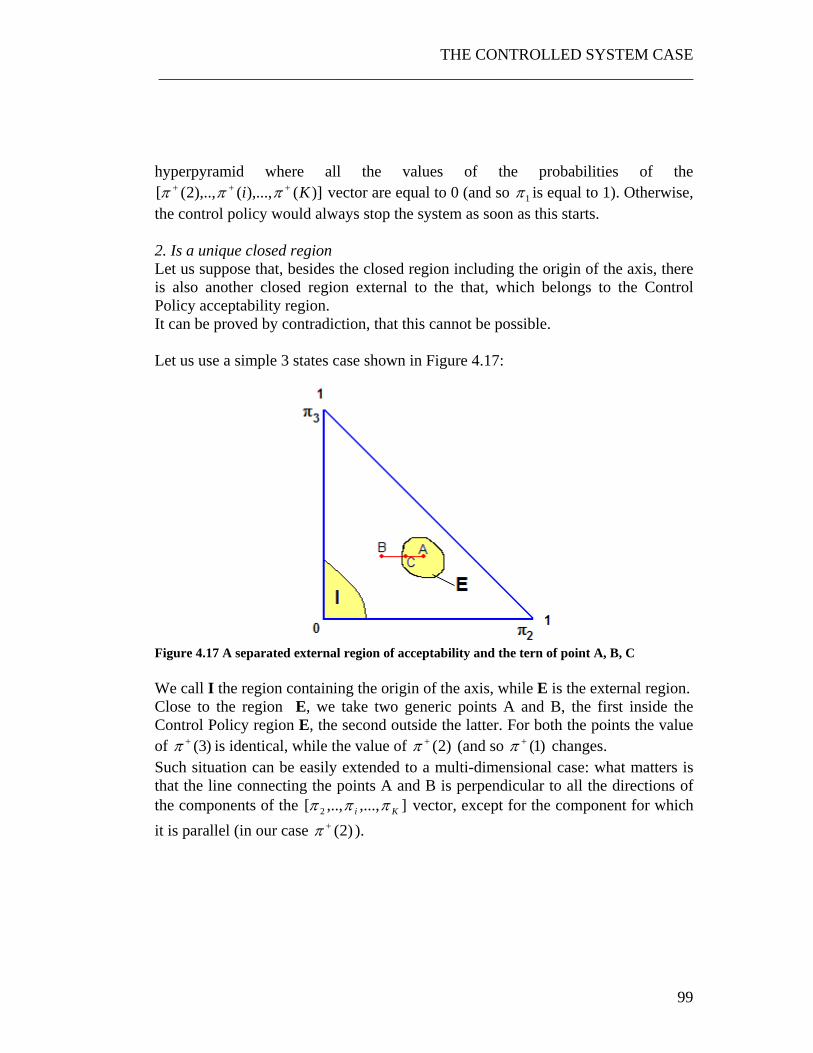
THE CONTROLLED SYSTEM CASE ___________________________________________________________________
99
hyperpyramid where all the values of the probabilities of the )](),...,(),..,2([ Ki +++ πππ vector are equal to 0 (and so 1π is equal to 1). Otherwise,
the control policy would always stop the system as soon as this starts. 2. Is a unique closed region Let us suppose that, besides the closed region including the origin of the axis, there is also another closed region external to the that, which belongs to the Control Policy acceptability region. It can be proved by contradiction, that this cannot be possible. Let us use a simple 3 states case shown in Figure 4.17:
Figure 4.17 A separated external region of acceptability and the tern of point A, B, C We call I the region containing the origin of the axis, while E is the external region. Close to the region E, we take two generic points A and B, the first inside the Control Policy region E, the second outside the latter. For both the points the value of )3(+π is identical, while the value of )2(+π (and so )1(+π changes. Such situation can be easily extended to a multi-dimensional case: what matters is that the line connecting the points A and B is perpendicular to all the directions of the components of the ],...,,..,[ 2 Ki πππ vector, except for the component for which it is parallel (in our case )2(+π ).

CHAPTER 4 ___________________________________________________________________
100
Let us suppose that the system state probability vector π+, after a sequence of observations, lies in a point C next to the border of the E region and on the line connecting A and B. Let us call 1μ the mean of the probability density function of the quality of the parts of the first state. In order for π+ to jump from the point C to the point A an observation y far from
1μ is necessary (the probability )1(+π must decrease). In the opposite case, in order for π+ to jump from the point C to the point B an observation closer to 1μ is required. This means that, using a control policy with a separate region would bring to the paradoxical situation where, given an identical sequence of past observations, the controller keeps the system working if a new ‘bad’ observation (far from 1μ ) is recorder while it stops it if a ‘good’ one is observed. It would be like using a control chart that considers as “out-of-control” an observation close to the target value, while it considers as normal an observation far from the latter. This type of policy is clearly not optimal, because we can always find a better policy which takes the same identical decisions of the first given any sequence of observations, with the only exception of the forementioned situation where it would keep the system working even in the case where the ‘good’ observation is recorded (an so it would not lose the consequent benefit associated to this action). In order not be in such a situation, the point B should be included in the control policy region, but if we keep iterating with the same example, the only way not to be in the same situation is that the region E should be connected to the region I. 3. Has partial derivatives always bigger then 0; 4. Does not have holes inside it Looking at the Figure 4.18 it is easy to see that if those two properties were not respected we could easily find a set of points A, B and C for which the same conditions explained in the point 2. are satisfied. The only way to avoid this contradiction is that the properties 1.,2.,3. and 4. are all respected.
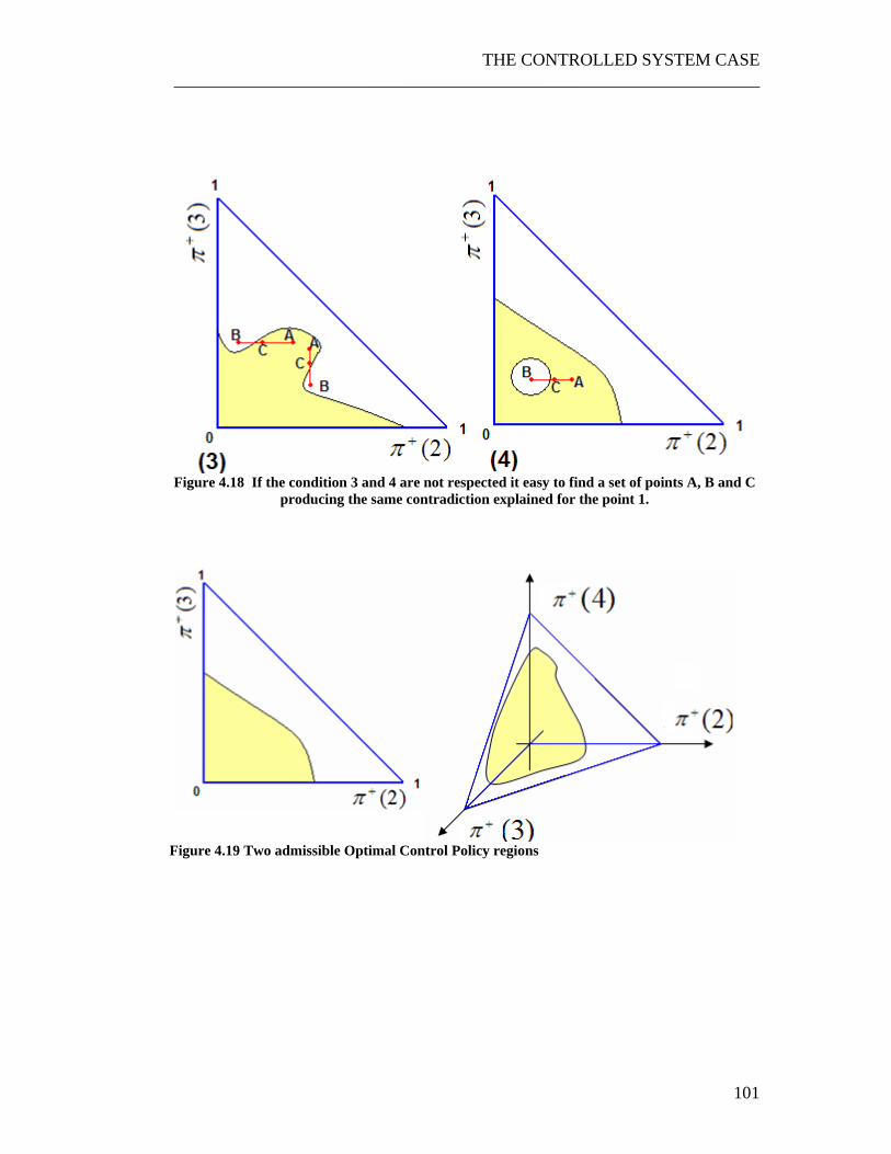
THE CONTROLLED SYSTEM CASE ___________________________________________________________________
101
Figure 4.18 If the condition 3 and 4 are not respected it easy to find a set of points A, B and C
producing the same contradiction explained for the point 1.
Figure 4.19 Two admissible Optimal Control Policy regions
Chapter 5
Solution techniques 5 In the previous Chapter we got to the conclusion that the system controller can take cost optimal decisions based on the a posteriori probability vector and that the optimal control policy region has a fairly simple structure. The problem to solve now is the research of such optimal policy. In the following Chapter we will combine the model used to study the interaction of the controller with the system, with the properties of the Optimal Control Policy Region (OCPR) developed in the Section 4.5 . To summarize, in the Section 4.5 we had concluded that the only thing required to solve the problem for the controlled system case is to find a way to associate to a given control policy the set of functions )](...)()([)( 21 npnpnpnp K= . In fact, if we have the set of functions )(np we can create the usual Markov chain and build the ARTP matrix of a deteriorating system controlled with a specific control policy. Using the usual algorithm we can thus evaluate the Average Cost associated to that control policy, and start the iterative approach that will eventually lead to the research of the optimal control policy. The target of this Chapter is to find a structured way to calculate this set of functions given a control policy, and to figure out a method to make the research of the optimal control policy as simple as possible. The Figure 5.1 shows the sequence of the operations necessary to solve the problem for the controlled system case and highlights the block the we are currently missing: the link between the control policy and the )(np vector.
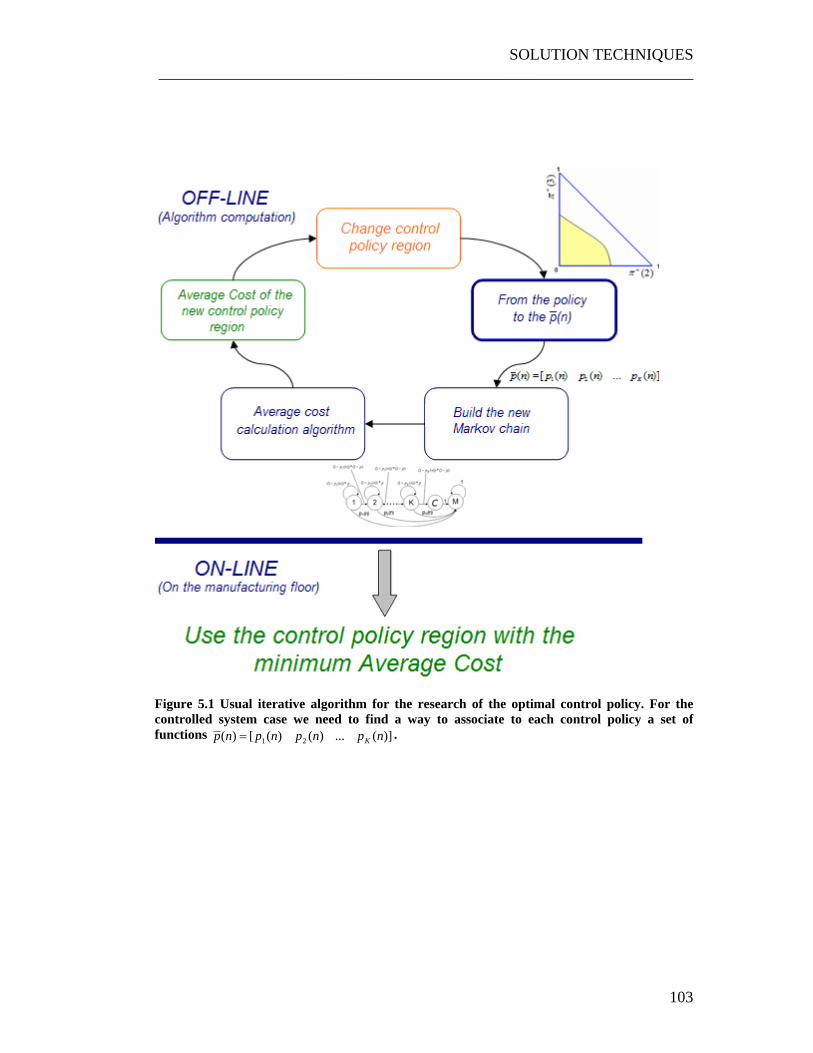
SOLUTION TECHNIQUES ___________________________________________________________________
103
Figure 5.1 Usual iterative algorithm for the research of the optimal control policy. For the controlled system case we need to find a way to associate to each control policy a set of functions )](...)()([)( 21 npnpnpnp K= .

CHAPTER 5 ___________________________________________________________________
104
5.1 From the control policy to the set of functions )](...)()([)( 21 npnpnpnp K=
The functions )(np are the probabilities that the system controller decides to stop the system at a time n, given that the system is in a given state i. For example )50(3p is the probability that the system controller would stop the system at the 50th time step if the system is in the third state. As we said, the system controller bases his decision on the a posteriori probability vector. His decision rules are also pretty simple: if the a posteriori vector lies in the control policy acceptability region he lets the system work, otherwise he stops it and starts maintenance. Moreover, as proved, the optimal decision rule is stationary i.e. it does not depend on the time. The system controller will just keep calculating the +π vector after every new observation check if the vector lies in the same control policy region, and start maintenance if the value lies outside. Let us now focus on the +π vector, i.e. the estimation that the system controller has about the true system state. Such value is calculated through the Formula ( 4.18) and using an iterative approach, shown in Figure 4.12 Algorithm for the computation and updating the system state vector. We can say that the +π vector, depending on the history of the observations, is a random variable. There are two sources of randomness affecting such value: the dynamic of the system (the system jumps from two adjacent states a random way) and the probability density function of the quality of the parts (given a state, the quality output is a random variable). We can so create a random variable +Π n defining the value of the +π vector at a time step n: given all the possible sequences of observations (in this case, n observations) +Π n is the realization of one these sequences. Since +π is a vector,
+Π n is a vector as well, i.e. )](...)(...)1([ Ki nnnn++++ ΠΠΠ=Π .
Associated to the +Π n vector, we can also create its probability density function:
)(~ ++ ΠΠ nnn ξ
( 5.1 )

SOLUTION TECHNIQUES ___________________________________________________________________
105
In this case, since +Π n is a vector, and his values are correlated, we will call (.)nξ the Joint Probability Density Function of +Π n . (JPDF). We can think about this function in the following way: let the system work for an infinite number of maintenance cycles. For each cycle, watch the +π vector that the controller has built at time n and record it: this is just one of the possible values of
+Π n . Given the infinite number of +Π n vectors recorded, you can build the (.)nξ function.
Having (.)nξ , we can answer to common questions like: what is the probability that
5.0)2(0 ≤Π≤ +n ? What is the probability that 5.0)2()1( ≥Π+Π ++
nn ? Or, more generically, what is the probability that Θ∈Π +
n with Θ being a generic region in the space Ω 7 of all the possible value of +Π ? All these question can be answered calculating the integral of the Joint Probability Density Function (.)nξ over the forementioned Θ regions:
∫Θ
+ Θ=Θ∈Π dP nn (.) )( ξ
( 5.2 )
The Figure 5.2 may help understand what we are doing:
1. We can define an arbitrary region Θ in the space Ω of the values of +Π . Since the sum of the element of +Π n has to be equal to 1, we can always describe such vector using K-1 components. So, if )]3()2()1([ ++++ ΠΠΠ=Π nnnn like in the example, we can use only )2(+Π n and )3(+Π n to describe it.
2. We build the Joint Probability Density Function )( +Π nnξ
3. The probability )( Θ∈Π+nP is given by the integral of the JPDF
)( +Π nnξ over the region Θ : ∫Θ
+ Θ=Θ∈Π dP nn (.) )( ξ
7 As we know, this region s the ‘hyperpyramid’ of the values of the a posteriori probability vector.

CHAPTER 5 ___________________________________________________________________
106
Figure 5.2 Creation of a region and calculation of the integral of the JPDF. We can even go beyond that. Let us take the function (.)nξ and condition it on a specific state. In other words, we want to find the probability density function of +Π n , given that the system is in a specific state r at time n. We can think about this calculation in the following way: let the system work for an infinite number of maintenance cycles. For each cycle, look at the +π vector that the controller has built at time n and inspect the machine state. If the machine state is r, record the value. Given the infinite number of +Π n vectors recorded, you can build the ))(|(. rnsn =ξ function.

SOLUTION TECHNIQUES ___________________________________________________________________
107
In this case, we can thus write that:
))(|(~ rnsnnn =ΠΠ ++ ξ
( 5.3 )
Again, with this Joint Probability Density Function we may ask the same questions we have been talking about before. But in this case, we may also find the answer to a very useful question. As we said, the control policy that the controller uses is just a region of acceptability in the space Ω of the a posteriori vector. The probability )(npi is nothing but the probability that the a posteriori vector at the time n will lie in the non-acceptability region, if the real system state at time n is i. In mathematical terms, if we call Θ the non-acceptability region we get:
))(|()( rnsPnp ni =Θ∈Π= +
( 5.4 )
But this value, like before, can be easily calculated as the integral of the Joint Probability Density Function of ))(|(. rnsn =ξ over the region Θ . In other words:
Θ== ∫Θdrnsnp nr ))(|(.)( ξ
( 5.5 )
The values of the probabilities vector )(np can thus be calculated performing an integral of the Joint Probability Density Functions ))(|(. rnsn =ξ , for each
],1[ Kr ∈ and each ],1[ WTLn ∈ , over the non-acceptability region. In other words, we would do same thing described in the Figure 5.2 for each state and time step, with Θ being the non-acceptability region. We will show in the following chapters how the JPDF ))(|( rnsnn =Π +ξ can be theoretically found, and we will provide a numerical algorithm for the research of these functions and the solution of the integral in the Equation ( 5.5 ).
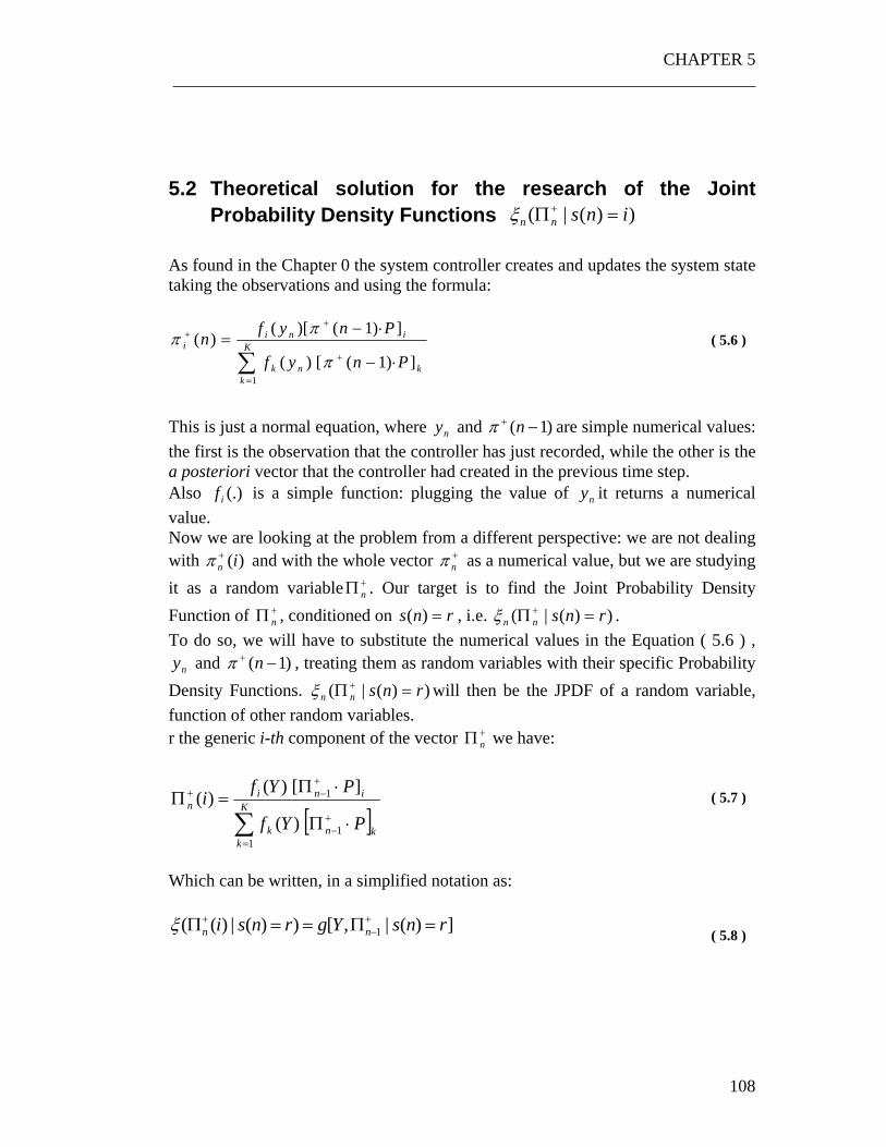
CHAPTER 5 ___________________________________________________________________
108
5.2 Theoretical solution for the research of the Joint Probability Density Functions ))(|( insnn =Π+ξ
As found in the Chapter 0 the system controller creates and updates the system state taking the observations and using the formula:
∑=
+
++
⋅−
⋅−= K
kknk
inii
Pnyf
Pnyfn
1]) 1() [(
]) 1()[()(π
ππ
( 5.6 )
This is just a normal equation, where ny and )1( −+ nπ are simple numerical values: the first is the observation that the controller has just recorded, while the other is the a posteriori vector that the controller had created in the previous time step. Also (.)if is a simple function: plugging the value of ny it returns a numerical value. Now we are looking at the problem from a different perspective: we are not dealing with )(in
+π and with the whole vector +nπ as a numerical value, but we are studying
it as a random variable +Π n . Our target is to find the Joint Probability Density Function of +Π n , conditioned on rns =)( , i.e. ))(|( rnsnn =Π +ξ . To do so, we will have to substitute the numerical values in the Equation ( 5.6 ) ,
ny and )1( −+ nπ , treating them as random variables with their specific Probability Density Functions. ))(|( rnsnn =Π +ξ will then be the JPDF of a random variable, function of other random variables. r the generic i-th component of the vector +Π n we have:
[ ]∑=
+−
+−+
⋅Π
⋅Π=Π K
kknk
inin
PYf
PYfi
11
1
) (
]) [()(
( 5.7 )
Which can be written, in a simplified notation as:
])(|,[))(|)(( 1 rnsYgrnsi nn =Π==Π +−
+ξ ( 5.8 )

SOLUTION TECHNIQUES ___________________________________________________________________
109
Where g is the function in the Equation ( 5.7 ). The JPDF of the vector +Π n is given by the combination of all the single components )(in
+Π with ],1[ Ki ∈ . We can thus rewrite:
⎥⎥⎥⎥⎥⎥
⎦
⎤
⎢⎢⎢⎢⎢⎢
⎣
⎡
=Π
=Π
=Π
==Π
+
+
+
+
))(|((...
))(|)((...
))(|)1((
))(|(
rnsK
rnsi
rns
rns
n
n
n
n
ξ
ξ
ξ
ξ
( 5.9 )
To find the expression of ))(|)(( rnsinn =Π +ξ , we need to find the probability density functions of the variables nY , +
−Π 1n with the condition that .)( rns = We will then use appropriate techniques to derive the expression of the Probability Density Function ))(|)(( rnsinn =Π +ξ starting from those Probability Density Functions.
nY is the most simple: if the system at time n is the state r, then the observation at time n is a random variable distributed like the probability density function of the quality of the parts for the state r. Formally:
)(~ YfY r ( 5.10 )
As for +
−Π 1n , things are not as simple. The +
−Π 1n vector, is the random variable defining the a posteriori probability vector at time n-1 . Since we are imposing the condition rns =)( , the JPDF of this random vector has to written as:
))(|(~ 111 rnsnnn =ΠΠ +−−
+− ξ
( 5.11 )

CHAPTER 5 ___________________________________________________________________
110
Now let us look at the dynamic of the system: if we impose the system to be in the state r at time n, it means that at time n-1 the system could have been either in the state r or the state r-1 (if there was a transition during the previous time step). The JPDF ))(|( 11 rnsnn =Π+
−−ξ have thus to be a combination of both
))1(|( 11 rnsnn =−Π +−−ξ and )1)1(|( 11 −=−Π +
−− rnsnnξ . It can be shown in Appendix III that:
)1)1(|( ))1(|(
))(|(
11,111,
11
−=−Π+=−Π=
==Π+
−−−+
−−
+−−
rnsrns
rns
nnrrnnrr
nn
ξηξη
ξ
( 5.12 )
Using the same procedure, we may even extend the Equation ( 5.12 ) to the generic case where the deterioration does not follow a linear path, so there might be transitions between any of the states of the system. In this case we would have:
∑=
+−−
+−− =−Π==Π
K
lnnlnn lnsrns
11111 ))1(|( ))(|( ξηξ
( 5.13 )
Since in this document we are dealing with linear type of deterioration we will always use the Equation ( 5.12 ). However, as we will show at the end of the document, the Equation ( 5.13 ) will be useful to extend the model to more complex situations. Let us now focus on the solution of the probabilities lη . As said, ))(|)1((, rnslnsPrl ==−=η , where l can be any state (in our problem l can be either r or r-1). This conditioned probability can be found immediately through the Bayes’ theorem.
))(())1(() )1(|)(())(|)1((
rnsPlnsPlnsrnsPrnsrnsP
==−=−=
===− ( 5.14 )
Let us analyze the elements at the right of the Equation ( 5.14 ) singularly:

SOLUTION TECHNIQUES ___________________________________________________________________
111
))1(|)(( rnsrnsP =−= = rlART nP ,)]1([ − ( 5.15 )
i.e. the transition probability taken from the ARTP matrix.
))1(( lnsP =− = )(1 ln−π
( 5.16 )
i.e. the probability that the system is a generic state l at a time step n-1 This probability can thus be taken from the l-th element of the vector 1−nπ
))(( rnsP = = rARTnn nPr )]1([)( 1 −⋅= −ππ ( 5.17 )
Again, this probability can be found as the r-th element of the nπ vector. This vector is simply given by the product of the probability vector at the previous time step, multiplied by the )1( −nPART matrix. We thus get:
rARTn
nrlARTrl nP
lnP)]1([
)( )]1([
1
1,, −⋅
−=
−
−
ππ
η ( 5.18 )
In our case, since l=r or l=r-1 we get:
rARTn
nrrARTrr nP
rnP)]1([
)( )]1([
1
1,, −⋅
−=
−
−
ππ
η
rARTn
nrrARTrr nP
rnP)]1([
)1( )]1([
1
1,1,1 −⋅
−−=
−
−−− π
πη
( 5.19 )
It is easy to see that, as expected, 1,1, =+ − rrrr ηη Since there is no state before the first state, we also have that:
11,1 =η ; 01,0 =η
( 5.20 )
CHAPTER 5 ___________________________________________________________________
112
The combination of the Equations ( 5.19 ) and ( 5.12 ) gives the solution to the problem of the research of the ))(|( 11 rnsnn =Π+
−−ξ . This expression, combined with the Equations ( 5.10 ) and ( 5.7 ) will then give the final expression of the JPDF ))(|( rnsnn =Π +ξ , i.e. the solution to the problem we were trying to solve at the beginning of this section. But there is another problem: the Equation ( 5.19 ) requires the knowledge of the
1−nπ and of the )1( −nPART matrix, while the Equation ( 5.12 ) requires the
knowledge of the ))(|( 11 rnsnn =Π +−−ξ that we do not have.
In the next Chapter we will show an analytical iterative method to solve this problem, starting from the time step 0 and gradually solving the problem for all the following time steps.
SOLUTION TECHNIQUES ___________________________________________________________________
113
5.3 An iterative approach for the solution of the problem In the two previous subsections we have shown how it is possible to evaluate the probabilities )(npi solving the integral of the JPDF ))(|( rnsnn =Π+ξ over the control policy non-acceptability region. We have also shown a way to find the expression of ))(|( rnsnn =Π+ξ , which means that in theory we would be able to find the generic probabilities )(npi , just applying the right set of equations. The only problem is that the Equation ( 5.19 ) requires the knowledge of the 1−nπ and of the )1( −nPART while the Equation ( 5.12 ) requires the knowledge of the
))(|( 11 rnsnn =Π +−−ξ that we do not have.
In fact, to know the 1−nπ vector, we should have the set of matrices )(mPART with
]1,..., 1[ −∈ nm . In that case we may write:
∏−
=− =
1
001 )(
n
mARTn mPππ
This problem seems impossible to solve, because to build the generic )(mPART matrix8 it is necessary to have the probability vector )(mp which is what we are trying to calculate. However, we can use an iterative approach to overcome this hurdle. At time 0 we know exactly what is the system state, since ]0...01[0 =π . This means that we also know all the JPDFs ))0(|( 00 rs =Π +ξ with ],....,1[ Kr ∈ since the state at 0 is deterministic, the JPDFs will be constant and equal to
]0...01[ . We also know what is the )0(ARTP matrix. In fact, the controller will never stop the system immediately after maintenance (it would not make sense to restart maintenance immediately after maintenance has been finished). This means that
[ ]0...00)0( =p , and so PPART =)0( .
8 Please, see how the )(mPART
matrix is built in the Formula ( 3.18 ).

CHAPTER 5 ___________________________________________________________________
114
Knowing ))(|( 00 rns =Π +ξ , 0π and )0(ARTP , we can use the equations ( 5.19 ) ,(
5.12 ), ( 5.10 ) and ( 5.7 ) to find the JPDFs ))(|( rnsnn =Π +ξ with ],....,1[ Kr ∈ . We will then integrate those JPDFs over the control policy non-acceptability region to find the )1(p vector, and so the )1(ARTP matrix. The +
1π vector can be found with the Equation ( 5.17 ) as [ ])0(01 ARTP⋅=+ ππ . We can thus find the )1(p vector, and since we have both )1(ARTP and +
1π we can reply what done for the time step 2. If we go ahead using this same iterative procedure, we can thus calculate the whole )(np functions (with ]),1[ WTLn ∈ . The Figure 5.3 shows a scheme of how the explained method works. We have thus found a way to calculate the probabilities )(np associated to a given control policy iteratively, which means that we are also able to evaluate the Average Cost associated to a given control policy. However, there is still an open problem: how is it possible to evaluate the JPDF
))(|( rnsnn =Π +ξ given the expressions of ))1(|( 11 rnsnn =−Π +−−ξ ,
)1)1(|( 11 −=−Π +−− rnsnnξ and )(Yf r .
As the reader may understand, this is the typical problem of the calculation of the Joint Probability Density Function of a random variable which is a function of other random variables. There are different approaches to solve this problem, whose applicability depend on the complexity of the problem. In the next chapter we will make a short review of the existing methods for then focusing on the Monte Carlo approach.

SOLUTION TECHNIQUES ___________________________________________________________________
115
Figure 5.3 A scheme of the iterative method for the calculation of the )(np functions

CHAPTER 5 ___________________________________________________________________
116
Figure 5.4 A simple scheme of the calculation of the probabilities )(np .
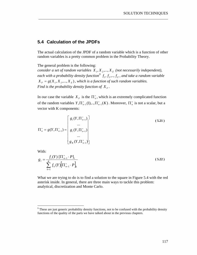
SOLUTION TECHNIQUES ___________________________________________________________________
117
5.4 Calculation of the JPDFs The actual calculation of the JPDF of a random variable which is a function of other random variables is a pretty common problem in the Probability Theory. The general problem is the following: consider a set of random variables ZXXX ,...,, 21 (not necessarily independent), each with a probability density function9 Zfff ,..,, 21 , and take a random variable
),...,,( 21 ZF XXXgX = , which is a function of such random variables. Find is the probability density function of FX . In our case the variable FX is the +Π n , which is an extremely complicated function of the random variables )(),..,1(, 11 KY nn
+−
+− ΠΠ . Moreover, +Π n is not a scalar, but a
vector with K components:
⎥⎥⎥⎥⎥⎥
⎦
⎤
⎢⎢⎢⎢⎢⎢
⎣
⎡
Π
Π
Π
=Π=Π
+−
+−
+−
+−
+
),(...
),(...
),(
),(
1
1
11
1
nK
ni
n
nn
Yg
Yg
Yg
Yg
( 5.21 )
With:
[ ]∑=
+−
+−
⋅Π
⋅Π= K
kknk
inii
PYf
PYfg
11
1
) (
]) [(
( 5.22 )
What we are trying to do is to find a solution to the square in Figure 5.4 with the red asterisk inside. In general, there are three main ways to tackle this problem: analytical, discretization and Monte Carlo.
9 These are just generic probability density functions, not to be confused with the probability density functions of the quality of the parts we have talked about in the previous chapters.
CHAPTER 5 ___________________________________________________________________
118
We will show how each of this methods works, and we will finally get to the conclusion that the best approach to solve our problem is a Monte Carlo based method.
5.4.1 Analytical solution There are common and relatively simple ways to calculate the PDF of the sum of independent and identically distributed random variables, using analytical expressions. As regards general functions of random variables things are not as simple. In general, for a one dimensional random variable which is a function of other random variables, there is an analytical approach for the research of the PDF. For example taken two independent random variables ),( 21 XX , both continuous and with probability density ),( 21 ff , and given the random variable
),( 21 XXgX F = , if g(.) is invertible and its inverse function has continuous partial derivatives, the density function of FX can be calculated considering a vectorial function of 1X and 2X , i.e.:
),( 21 XXgX F = first component
1XV = second component ( 5.23 )
If we are able to find:
),(11 VXhX F= ),(22 VXhX F=
( 5.24 )
and to write the Jacobian matrix of this transformation, there is a formula (that can be found in almost every Probability Theory book) through which it is possible to pass from the joint probability of ),( 21 XX to the joint probability of ),( VX F . The probability density function of F can thus be calculated using a marginalization approach (i.e. with an integral). Such procedure can also be extended to a n-dimensional random vector: instead of performing one integral, there are n-1 integrals to perform.
SOLUTION TECHNIQUES ___________________________________________________________________
119
Even for a relatively simple case (two independent variables ),( 21 XX ) this type of approach can be applied to a relatively small number of cases. What makes such approach difficult is the inversion of the g(.) function and the analytical solution of the marginalization integral. If we look at our g(.) we immediately realize that things are not as simple.
[ ]∑=
+−
+−
⋅Π
⋅Π= K
kknk
ini
PYf
PYfig
11
1
) (
]) [()(
( 5.25 )
Or
))(),...,(),...,1(,( 111 KiYgg nnn+
−+
−+
− ΠΠΠ= ( 5.26 )
• g(.) is a function of K+1 random variables, which means that we should be able to invert and integrate K functions
• g(.) is a function of correlated random variables: ))(),...,(),...,1(( 111 Ki nnn+−
+−
+− ΠΠΠ
are correlated since their sum must be equal to one. This means that we cannot apply the described method for independent random variables: there are other techniques for correlated random variables, but they significantly increase the complexity of the problem.
• The complexity of the (.)g function makes it very likely that, even if we managed to write the marginalization integral, we will not be able to find an analytical solution to the latter.
• The last problem is that, supposing that we were able to find the analytical expression of ))(|( rnsnn =Π +ξ , no one can guarantee that we will be able to find an analytical solution to the integral Θ== ∫Θ
drnsnp nr ))(|(.)( ξ . Since
this is a multidimensional integral, there are very few cases (special function and special integration regions) where an analytical solution to this integral can be found.
This set of considerations makes it unlikely that the problem may ever find an analytical solution, even though the authors do not exclude the possibility that for special cases, a complete or approximated analytical solution may be found. Since the target of this work is to provide a viable way to find the optimal control policy, regardless of the complexity of the problem, we will explore different ways to do this.

CHAPTER 5 ___________________________________________________________________
120
5.4.2 Discretization solution
A possible approach is a discretization solution. In this case we do not research the analytical expression of the function ))(|( rnsnn =Π +ξ , but we calculate a discretized expression of the latter. The solution is the following: We discretize the probability density function of the quality of the parts in an arbitrarily big number of discrete pieces. We also discretize the space Ω of all the values of the +Π Vectors: since this is a generic Nℜ space, we will have a discrete number of hypercubes (cubes if N=3, squares if N=2), that build the whole Ω like bricks. For each value of the discretized Y and +
−Π 1n we evaluate the (.)g function and check in which discretized hypercube it lies. Since Y and +
−Π 1n are independent, we add a probability P(Y) P( +
−Π 1n ) to this hypercube. We keep iterating until all the combinations of Y and +
−Π 1n have been calculated. We will eventually get a discretized expression of the ))(|( rnsnn =Π +ξ , i.e. a set of hypercubes building the Ω region of +Π n to each of which there is a specific probability associated. The calculation of the probabilities )(np is thus given by the sum of all the probabilities of the hypercubes included in the control policy non-acceptability region. The Figure 5.5 summarizes what has been explained: as clear, the set of the operations that are run in the algorithm are identical to the analytical case in Figure 5.4. The only difference is that in this case we do not look for the exact expression of the
))(|( rnsnn =Π +ξ , but we calculate it only for a given number of discrete values. The big problem of this approach is that the computational burden required to solve it increases severely as the complexity of the problem increases. Suppose, for example, that we discretize the space of the Y in 10 parts and the space of the +Π n in 10 parts for each component of the vector (i.e. 10 parts for each state). This means that, for each new state that we add, the number of calculations required increases by 10 (an order of magnitude!). It is reasonable to think that for large number of states the computational burden required by this method would increase too much, thus limiting this approach to relatively simple ,problems (small number of states).
SOLUTION TECHNIQUES ___________________________________________________________________
121
There are however ways to simplify the problem using approximations that can make the solution more viable: for example we may limit the calculations only for those hypercubes of the +
−Π 1n for which there is a probability bigger then a limit values (if the probability is too small, it does make sense to perform a calculation that will not significantly affect the final result).
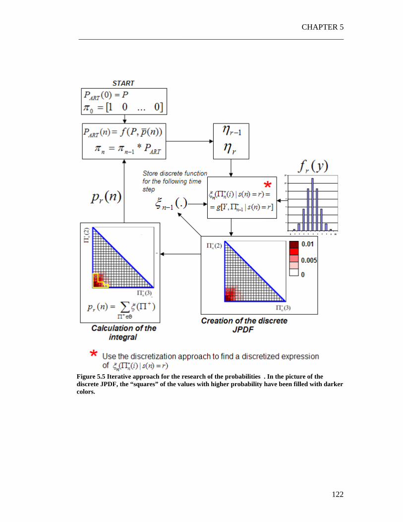
CHAPTER 5 ___________________________________________________________________
122
Figure 5.5 Iterative approach for the research of the probabilities . In the picture of the discrete JPDF, the “squares” of the values with higher probability have been filled with darker colors.
SOLUTION TECHNIQUES ___________________________________________________________________
123
5.5 The Monte Carlo approach As seen in the previous chapters, the main problem of applying the iterative method for the research of the Average Cost of a given control policy is the fact that the actual calculation of the JPDF of the +Π n , given the PDF of Y and the JPDF of +
−Π 1n is very difficult to perform analytically. The discretization approach provides a viable way to find a solution, but it does not guarantee reasonable computational times, unless the problem is relatively simple and serious improvement are used to optimize the algorithm. In this chapter we will show the use of a Monte Carlo based model to solve both the problem of the research of the function ))(|( rnsnn =Π +ξ and its integration over the control policy region. As we will prove, the use of a Monte Carlo based method will help to solve both this problems in a unique procedure. Through this approach we will be able to find an approximated expression of the probability vector )(np .
5.5.1 The general approach Let us take two generic random variables 1X and 2X with probability density 1f and 2f 10, and let us consider a random variable ),( 21 XXgX F = . There is no hypothesis about the type of distribution of 1X and 2X , and the two variables can also be correlated. The pdf of FX could be built generating random numbers from the distribution of
1X and 2X and calculating the function ),( 21 XXgX F = for each of those numbers. We will thus generate random numbers from the distribution of FX . Once a large enough sample of random numbers of ),( 21 XXgX F = has been generated, the pdf of FX can be estimated fitting the generated random points with a probability density function. Suppose now that we want to find the probability that the variable FX is bigger than a given value α . In this case we should integrate the calculated pdf over all the values bigger then α . 10 Please, do not confuse this pdf with pdf of the quality of the parts. This is just a generic example with generic random variables.

CHAPTER 5 ___________________________________________________________________
124
An easier way to do so is to use the random points generated through the Monte Carlo method and check how many of them lie in the region where α>FX . The probability )( α>FXP can thus be estimated as:
TOT
FF L
LXP αα >=> )(ˆ ( 5.27 )
Where )( α>FXL is the number of random points lying in the region where α>FX and TOTL is the total number of generated random points. In general we can use this approach for any function (.)g , for any number of random variables and for any region.
5.5.2 The approach for our problem Let us now consider the problem we are studying: in this case the variable FX is the multi-dimensional variable +Π n , the function (.)g is defined by the Equations ( 5.21 ) and ( 5.22 ), while the region of integration is the control policy non-acceptability region Θ . Like said, we can generate an arbitrarily large number of random points (or vectors) from the distribution of +Π n , and we can estimate the probability )(npi as:
TOTni L
LPnp n )()(ˆ)(ˆ Θ∈Π+ +
=Θ∈Π=
( 5.28 )
Now, )(ˆ npi is just an estimation of )(npi , but we can easily keep the under control the difference between the real value of such probability and its estimation. Looking at the problem, it is easy to notice that the number of points lying in the
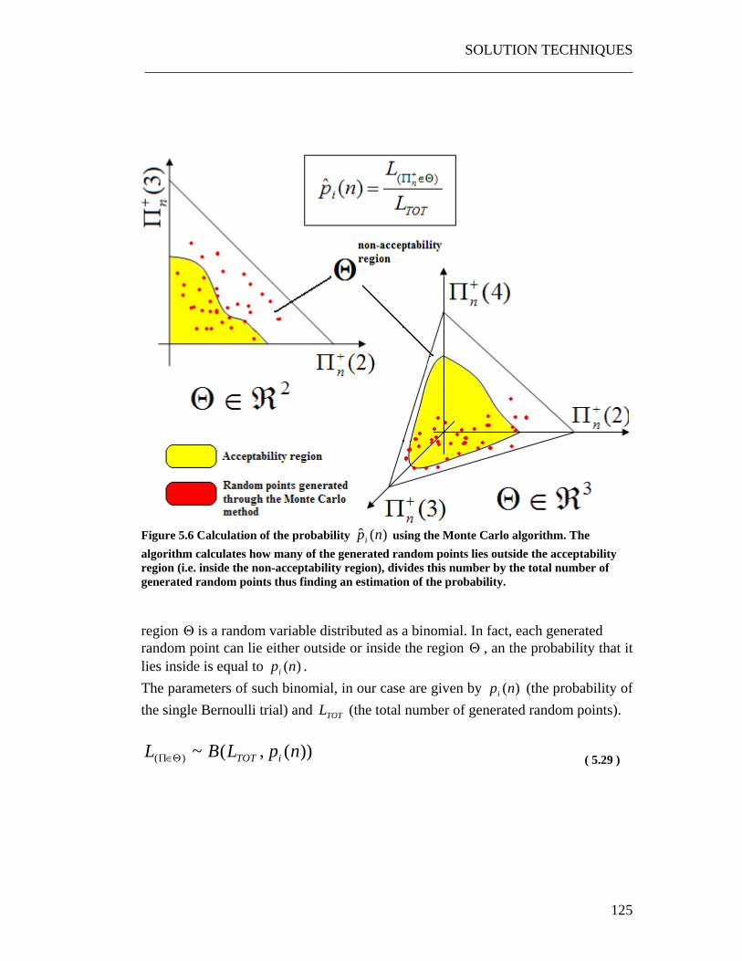
SOLUTION TECHNIQUES ___________________________________________________________________
125
Figure 5.6 Calculation of the probability )(ˆ npi using the Monte Carlo algorithm. The algorithm calculates how many of the generated random points lies outside the acceptability region (i.e. inside the non-acceptability region), divides this number by the total number of generated random points thus finding an estimation of the probability.
region Θ is a random variable distributed as a binomial. In fact, each generated random point can lie either outside or inside the region Θ , an the probability that it lies inside is equal to )(npi . The parameters of such binomial, in our case are given by )(npi (the probability of the single Bernoulli trial) and TOTL (the total number of generated random points).
))(,(~)( npLBL iTOTΘ∈Π ( 5.29 )
CHAPTER 5 ___________________________________________________________________
126
As well-known for large TOTL a Binomial Distribution converges to a Normal Distribution with mean pLTOT * and variance ))(1(*)(* npnpL iiTOT − . In other words:
)))(1)((),(()(
npnpLnpLNL iiTOTiTOTn
−≈Θ∈Π+
( 5.30 )
Where N is the normal distribution. We can thus say that:
)1;0())(1)((
)( NnpnpL
pLL
iiTOT
TOTn ≈
−
−Θ∈Π+
( 5.31 )
Dividing everything by TOTL we get:
)1;0())(1)((
)()(
N
Lnpnp
npL
L
TOT
ii
iTOT
n
≈−
−Θ∈Π+
( 5.32 )
If we define TOT
i L
Lnp n )()(ˆ Θ∈Π+
= we have:
)1;0())(1)((
)()(ˆN
Lnpnp
npnp
TOT
ii
ii ≈−
−
( 5.33 )
This means that the parameter TOT
i L
Lnp n )()(ˆ Θ∈Π+
= is an unbiased estimator of )(npi
and moreover the difference between the estimator and the real probability )(npi is a random variable with a Normal Distribution whose variance can be kept under control changing the number TOTL .

SOLUTION TECHNIQUES ___________________________________________________________________
127
The function ))(1)(( npnp ii − has a maximum for 5.0)( =npi for which ))(1)(( npnp ii − =0.25.
In the worst case (when 5.0)( =npi ), the variance of the difference between the
estimator and the real parameter is so given by TOTL25.0 , i.e. the variance decreases
hyperbolically as TOTL increases. This means that, for every state and time step we can find an unbiased estimation of the probability )(npi and moreover we can easily keep the difference between the estimation and the real parameter under control by changing the TOTL parameter.
For example we could say that the minimum variation of interest of the )(npi with its estimation has to be smaller then a given δ with a level of confidence of the 95%. We may call δ as maximum difference of interest.
%95))(ˆ)(( <≤− δnpnpP ii We can so choose a TOTL for which 05.0=δ with a level of confidence of the 95%. In the figure below it is shown that to get such a difference with such level of confidence, a number TOTL =800 is sufficient in the worse case ( )(npi ).
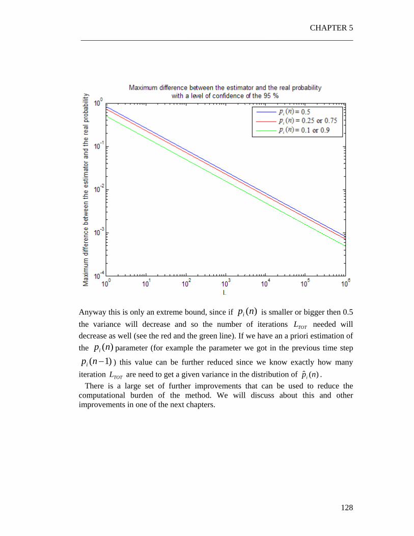
CHAPTER 5 ___________________________________________________________________
128
Anyway this is only an extreme bound, since if )(npi is smaller or bigger then 0.5 the variance will decrease and so the number of iterations TOTL needed will decrease as well (see the red and the green line). If we have an a priori estimation of the )(npi parameter (for example the parameter we got in the previous time step
)1( −npi ) this value can be further reduced since we know exactly how many iteration TOTL are need to get a given variance in the distribution of )(ˆ npi . There is a large set of further improvements that can be used to reduce the computational burden of the method. We will discuss about this and other improvements in one of the next chapters.
SOLUTION TECHNIQUES ___________________________________________________________________
129
Observations about the method The huge advantage of this method is that it is able to perform the integral of JPDF immediately, without finding the JPDF itself. Moreover, we can always keep the problem under control choosing a number TOTL such that the difference between the estimated probability and the probability itself is always kept under a value δ . Another advantage is that this method does not change or become more complex as the dimensions of the problem increases (i.e. the number of states K increases). In fact, regardless of the number of states and so regardless of the number of dimensions of the region Θ , the TOTL required to achieve a given δ remains unvaried (the random points can only be in or out the control policy region, regardless of the dimension of the problem).
5.5.3 Application of the Monte Carlo method in the iterative algorithm The application of the Monte Carlo method gives also significant advantages when applied in the iterative algorithm shown in the Section 5.3 . As shown in the Figure 5.7, we do not need to calculate a JPDF of +Π n and use it in the following time steps. We only need to store in memory the random points that have been generated from the JPDF of +Π n and use them in the following time step to calculate for the calculation of the new JPDF. On these grounds, everything remains the same as in the original analytical method shown in Figure 5.4, with the only difference that in this case we are not dealing with density functions but with numerical values randomly extracted from those functions. As shown in Figure 5.7, the algorithm will perform the same set of operations described for the theoretical algorithm: the only difference is that instead of looking for an analytical expression of the ))(|( rnsnn =Π +ξ , the algorithm is able to

CHAPTER 5 ___________________________________________________________________
130
Figure 5.7 Application of the Monte Carlo method to the iterative algorithm for the research of the )(np vector. The box with the red asterisk is the loop for the generation of random +Π n described in Figure 5.8. generate an arbitrarily large number of random points extracted from this distribution and use them to solve (numerically) the integral for the calculation of the probability )(ˆ npi .

SOLUTION TECHNIQUES ___________________________________________________________________
131
The generation of the random points +Π n (box with the red asterisk in Figure 5.7) is described in Figure 5.8. Each loop is able to generate one random point ) ( z
n+Π from ))(|( rnsnn =Π +ξ ,
where (z) is an index of the generic z-th loop.
Figure 5.8 Loop for the generation of random vectors +Π n from ))(|( rnsnn =Π +ξ . This is the box with the red asterisk in Figure 5.7.

CHAPTER 5 ___________________________________________________________________
132
First, a random number γ is generated from )(yf r . After that, a random vector ) (
1z
n+
−Π is generated using the Equation ( 5.12 ). Since this equation requires the density functions ))1(|( 1 rnsn =−Π +
−ξ and )1)1(|( 1 −=−Π +
− rnsnξ , the algorithm uses the two random vectors generated from these functions in the previous time step (n-1) during the z-th loop. The reason why we use the values generated during the z-th loop of the previous time step is just to give more order to the algorithm. In theory we could pick any of the TOTL values, what matter is that in the algorithm we use all of them11. The algorithm is so able to generate a cloud of random points in the space of the
+Π vector, to use them for the calculation of the probabilities )(ˆ npi and to store them for the following time step. If this algorithm is repeated for all the time steps it can give the values of the )(np function. The only thing we have to do is to plug this vector of function in the algorithm in Figure 5.1 and evaluate the Average Cost of the control policy. This means that with the Monte Carlo approach we have found a viable way to evaluate the cost of a given control policy.
5.5.4 Monte Carlo for the research of the optimal control policy Now that we have figured out how to calculate the probabilities )(np given a control policy, there is still the problem to understand how the optimal control policy has to be sought. What the Monte Carlo algorithm can do is to calculate the average cost, given a control policy defined through a region of acceptability and a region of non acceptability Θ . Given a large enough set of control policy region, the Monte Carlo algorithm can find which is the optimal one but there are still two open problems:
• The Monte Carlo method requires a significant computational burden which increases with the complexity of the problem. This limits the
11 If in the previous time step we have generated TOTL random vectors it is good to use all of them
to calculate the TOTL random vectors of the new time step. In fact, if we used the same value for more then once we would decrease the randomness of the Monte Carlo method, making it a little biased.
SOLUTION TECHNIQUES ___________________________________________________________________
133
number of control policies that can be explored to a relatively small number (depending on the time available to perform the computation)
• Even if we were able to accelerate this calculation, there would still be
the problem of understanding how the Ω region has to be explored in order to find the optimal control policy region, and how we can say that a control policy region is actually the optimal one.
In the following chapter we will present some numerical results and we will show how the properties of the JPDF of the +Π makes it possible to find a solution to both of these problems. In particular we will discuss the “Snake” shape of the JPDF and we will prove how this can seriously simplify the problem. In the last chapter, some possible improvements to the Monte Carlo method are also presented.
Chapter 6 Numerical results 6 In this Chapter we will present and discuss the numerical results of the method, trying to underline the properties that can be exploited to improve its performance. In particular, we will focus on two aspects: the properties of the Joint Probability Density Function of the +Π vector and the characteristics of the probability function vector )(np , showing how these properties can make the algorithm for the research of optimal control policy faster and more efficient.

NUMERICAL RESULTS ___________________________________________________________________
135
6.1 Numerical experiments on the JPDF The iterative method described in the Section 5.3 has been solved using the Monte Carlo approach explained in Section 5.5. The reason why we have preferred a Monte Carlo method to a discretization approach is because, as already mentioned, a discretization algorithm would require serious improvements to provide acceptable results in a reasonable period of time. The same thing is not true for the Monte Carlo approach which, even if open to a wide set of improvements, can give pretty good results and provide a deep insight of the problem without needing an excessive complication of the model. It is important to remember that in the Monte Carlo algorithm for the research of the Optimal Control Policy it is not necessary to find an expression of the JPDF, since the integral for the calculation of the )(np is directly performed using the Equation ( 5.28 ). The purpose of this Section is to understand, through numerical examples, which are the characteristics of the JPDF and if they can be exploited to improve the model. The algorithm has been developed using the commercial numerical software Matlab®; the graph shown in the pictures of this Chapter have been plotted using the same program. The algorithm, which has been entirely developed autonomously, executes the same set of operations described in the Section 5.3 and Section 5.5, summarized in the Figure 5.7 and Figure 5.8. The algorithm generates a cloud of random points from the JPDF of +Π for each state ],...,1[ Kr ∈ and each time step ],...,1[ maxnn = . In one of the following Chapters, we will show how the maxn is chosen. If the problem is one or two dimensional (i.e. K=2 or K=3)12, we can also visualize the JPDFs. For example if K=3, we can use two dimensions to indicate the coordinates )]3(),2([ ++ ΠΠ and the third dimension to plot the value of the JPDF
given a each set of coordinates )]3(),2([ ++ ΠΠ . For K=4 we cannot visualize the JPDF, but we can plot the cloud of points in the three dimensional space and see where they lie and how they are distributed in the space. For K>4 no possible visualization of the JPDF is possible.
12 Please remember that, since the sum of the element in the +Π must be equal to one, this vector can be entirely described in a K-1 dimensional space.

CHAPTER 6 ___________________________________________________________________
136
We have thus decided to present two set of experiments, one for a K=3 and one for K=4. The first will give us an immediate vision of the shape of the JPDF and will be used afterwards to investigate the correlation between this function and the control policy. The second will instead help us to find the properties of the shape of the JPDF.
6.1.1 A three states system The chosen system has K=3 states and a probability of transition p=0.05. The experiment have been performed generating 5000=TOTL random points.
Variable Value
K 3
p 0.05
TOTL 5000
We do not need to specify a Crash cost or a Maintenance Cost or Time: here we are just looking for the JPDF of +Π and not for an optimal control policy. The target of this first experiment is to present to have a first view of how a JPDF of the +Π looks like and to show that, if TOTL is sufficiently big, the shape of the JPDF does not change significantly performing different experiments (thus guaranteeing a better reliability of the results if TOTL is big). In order to visualize the JPDF, we have divided the space of the )]3(),2([ ++ ΠΠ values in a grid of squares, counted how many points lie in each square, divided this number by the total number of generated points, thus finding the probability

NUMERICAL RESULTS ___________________________________________________________________
137
Figure 6.1 Calculation of JPDF starting from the random cloud of point associated to each square. Repeating the same operation for each square we have finally come up with a complete (clearly, discretized) expression of the JPDF. The results are presented using a color scale where the red means high probability while the blue is low (or zero) probability. We have repeated the experiment for two times to check if there is any significant difference in the shape of the JPDF. The results are shown in the next page. As clear, the shape of the JPDF is almost the same in the two cases. The considerations about why the JPDF has that shape and how it changes with the time n and the state r will be better discussed in the next Subsection.

CHAPTER 6 ___________________________________________________________________
138
Figure 6.2 A typical JPDF. The experiment has been repeated for two times: as clear the shape
of the JPDF remains almost the same.
NUMERICAL RESULTS ___________________________________________________________________
139
6.1.2 A four states system In this Subsection we will present results for a 4 states system. The target of this Subsection is to explore what is the typical shape of a JPDF and to understand intuitively why it has that shape. Having more degrees of freedom (3 instead of 2) will improve the vision of the problem making it simpler to discover properties in the JPDF. First of all it is necessary to remember that there is a JPDF of +Π for each state and for each time step. The function ))(|( rnsn =Π +ξ , is the generic JPDF when the system is in the state r at a time n. In other words if the real system at a time n is in the state r the +Π vector that the controller will observe is a random variable (vector), distributed as
))(|( rnsn =Π +ξ . As the reader may intuit, the ))(|( rnsn =Π +ξ will change with the state r and with the time n. However, there are several open questions:
• Is there a recurrent shape of the JPDFs? • How do the JPDFs change as the parameters of the problem change? • Is there any correlation between the shape of the JPDF for different states r? • May we expect some kind of time evolution in the shape of the JPDF, as n
increase? In this Subsection we will try to find an answer to all of these question, using a set of different experiments. We have chosen to explore three different situations, with different parameters. What we will change are the probability of transition p and the probability density of the quality of the parts for the different states. The probability density functions are Gaussian, with different mean and average.

CHAPTER 6 ___________________________________________________________________
140
Figure 6.3 Set of input parameters for the three cases. The case 2 has a different p parameter, while the case 3 has a different set of the Probability Density Function of the quality of the parts
NUMERICAL RESULTS ___________________________________________________________________
141
As shown in the figures, in the Case 2 we have same PDFs of the quality of the parts, but the parameter p changes (faster deterioration). The Case 3 has same the same p as in the Case 3, but the PDFs of the quality of the parts are different: there is low “overlapping” among the PDFs, i.e. when one of the PDFs has high values, the others have relatively small values and vice versa. For each Case we run the algorithm for the generation of the random cloud. The random cloud has been created for each state ]4,...,1[=r and for all the time steps ]30,...,1[=n . As already said, for the 3-dimensional case we are not able to see the JPDF, but looking at how the cloud of random points is distributed in the space we will get a lot of information about this function (high concentration of random points = high probability). In the following pages we will show a set of graphs, referring to each case, where the random cloud is represented for each state, and for n=1, 3, 5, 10. In this way we will have a complete view of the shape of the JPDF and we will understand how it changes with the state and with the time.
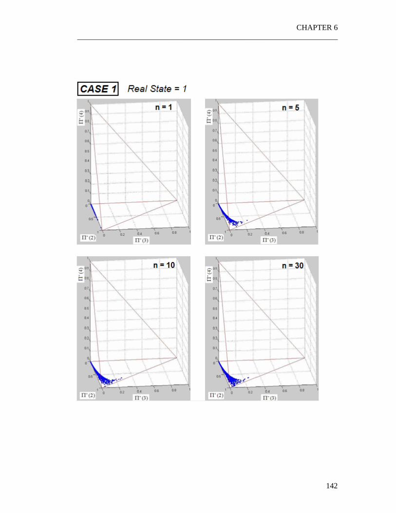
CHAPTER 6 ___________________________________________________________________
142
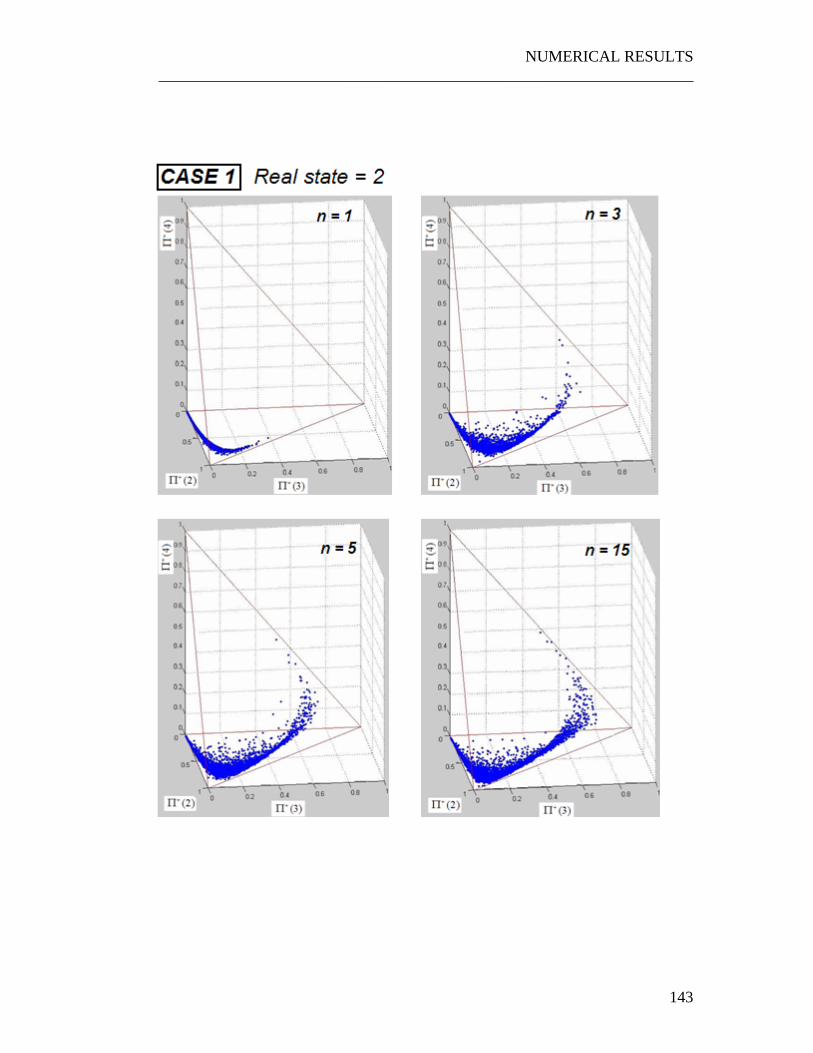
NUMERICAL RESULTS ___________________________________________________________________
143

CHAPTER 6 ___________________________________________________________________
144

NUMERICAL RESULTS ___________________________________________________________________
145

CHAPTER 6 ___________________________________________________________________
146

NUMERICAL RESULTS ___________________________________________________________________
147

CHAPTER 6 ___________________________________________________________________
148
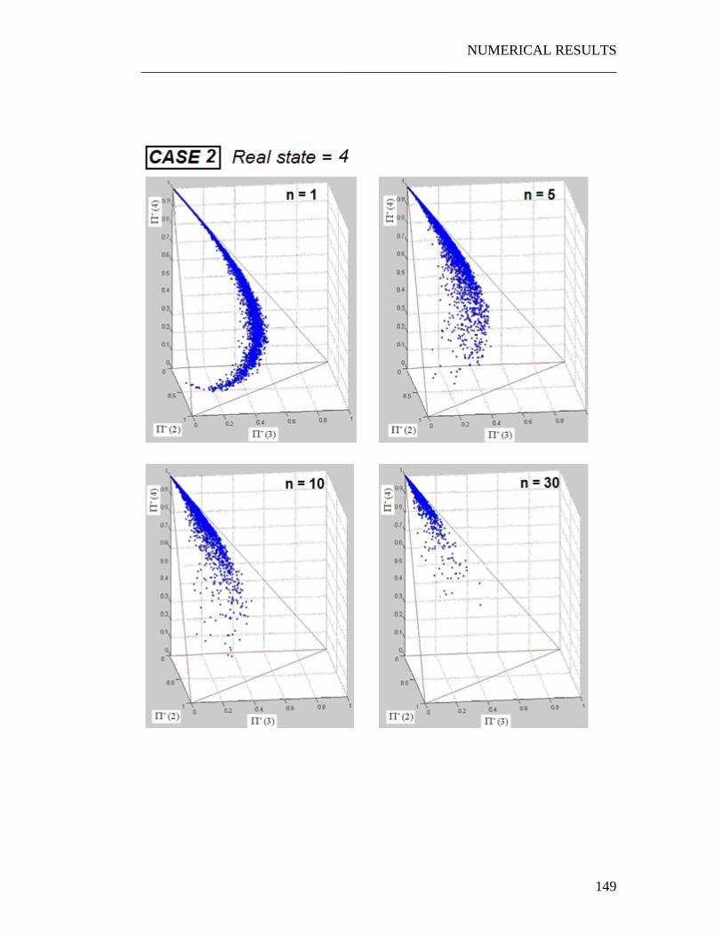
NUMERICAL RESULTS ___________________________________________________________________
149

CHAPTER 6 ___________________________________________________________________
150

NUMERICAL RESULTS ___________________________________________________________________
151
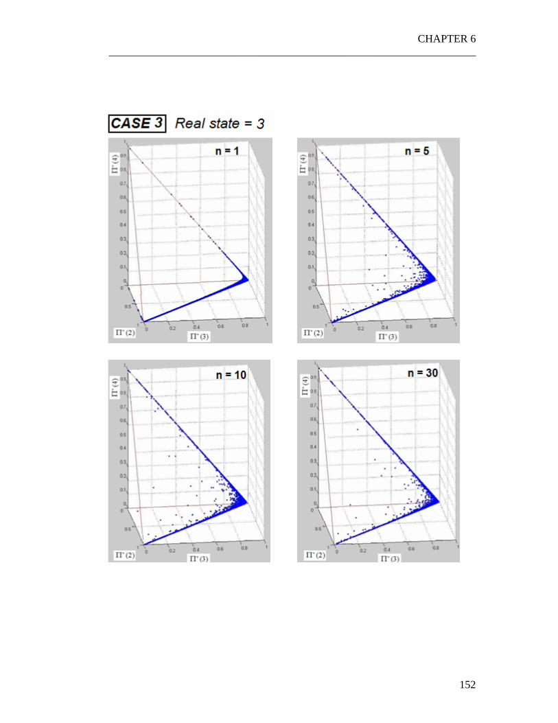
CHAPTER 6 ___________________________________________________________________
152
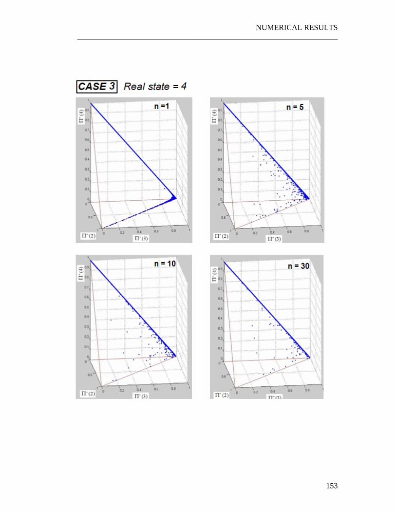
NUMERICAL RESULTS ___________________________________________________________________
153
CHAPTER 6 ___________________________________________________________________
154
6.2 Interpretation of the graphs As already said in different situations, the variable +
nπ represents the subjective vision of the system that system controller has created after gathering n observations since the beginning of the process. Since the observations are random, given a same state and a same time, the observer can have different values of +
nπ . This variable can thus be seen as a random variable, indicated by the sign +Π n . Roughly speaking, the JPDF of +Π n shows what the system controller is likely to believe if the real system is in a state r at a time n. It is important to remember that the four corner of the hyperpyramid is where the probability of one of the 4 states is equal to 1 (and the other equal to 0). The origin of the axes, i.e. the corner where
)2(+Π , )3(+Π , )4(+Π are equal to 0, is where )1(+Π is equal to 1.
6.2.1 The “Snake” shape It easy reasonable to think that, if the real system is in the generic state r the observer will assign a large probability to the state r and a small probability to the other states. In other words we may expect that if the real system is in the state r, the observer is “smart” enough to perceive it, and so most of the points will be concentrated near the corner where 1)( =Π + r . Looking at the graphs, this is actually what happens. However, we can notice that the they are not spread in a shapeless way around such corner, but the way they distribute themselves in the space has a clear pattern, which reminds the shape of a “snake”, leaving some spots in the space completely empty (with probability equal or very close to 0). This type of shape can also be observed in every graph, same regardless of the time n and of the state r. The interpretation of this phenomenon is the following. Since the deterioration of the system is linear and increasing from 1 to K, it is likely that the observer may be confused about adjacent states. On these grounds we may expect the +Π vector components to be different from zero only in 2 or 3 adjacent states, and to be null in the other components. If the highest probability is in the state r, for example, we may expect the states r-1 and r+1 to have non-zero probability as well, but we can be pretty sure that the probability of the states r-2 and r+2 will be smaller then the probability of the states r-1 and r+1. On these grounds, values of the a posteriori
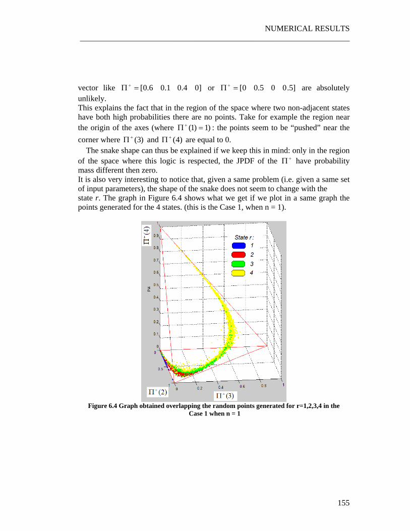
NUMERICAL RESULTS ___________________________________________________________________
155
vector like ]04.01.06.0[=Π + or ]5.005.00[=Π + are absolutely unlikely. This explains the fact that in the region of the space where two non-adjacent states have both high probabilities there are no points. Take for example the region near the origin of the axes (where )1)1( =Π + : the points seem to be “pushed” near the corner where )3(+Π and )4(+Π are equal to 0. The snake shape can thus be explained if we keep this in mind: only in the region of the space where this logic is respected, the JPDF of the +Π have probability mass different then zero. It is also very interesting to notice that, given a same problem (i.e. given a same set of input parameters), the shape of the snake does not seem to change with the state r. The graph in Figure 6.4 shows what we get if we plot in a same graph the points generated for the 4 states. (this is the Case 1, when n = 1).
Figure 6.4 Graph obtained overlapping the random points generated for r=1,2,3,4 in the
Case 1 when n = 1
CHAPTER 6 ___________________________________________________________________
156
As clear in the graph, the random points align themselves creating the typical snake shape, thus confirming the snake-shaped properties of the JPDF of the +Π . This shape seems to remain unchanged also when n increase: what changes is how the probability mass is distributed over this basic structure. This fundamental property of the JPDF can be exploited to reduce the complexity of the research of the optimal control policy, as we will show in a later Section.
6.2.2 Time evolution of the JPDF Another characteristic that can be observed in the graph is how they change with the time n. It looks like, as the time elapses, the cloud of points tend to “crawl”, going towards the upper corner where 1)4( =Π + . The reason why this happens is again related to the dynamic of the process: as the time elapses, the observer becomes more and more disposed to believe that the system is an of the more deteriorated states. So, even if the real system is for example in the first state, when n is big the controller is still likely to believe that the system is in a more deteriorated state. On these grounds, as n grows, most of the probability mass of the JPDF of +Π moves to the higher states. Another characteristic of the time evolution of the JPDFs is the fact that they tend to settle asymptotically to a given shape as the time n approaches infinity. Actually, as it can be observed in the graphs, the JPDF tend to settle very quickly (in some cases after only 10/20 time steps). This characteristic will be better discussed and exploited in the Section
6.2.3 Correlation with the PDFs of the quality of the parts In the Case 3 we have used a different set of PDFs of the quality of the parts for the four states. The main difference, as already observed in the Section 6.1 and as clear in the Figure 6.3, is that in the PDFs used in the case three are less overlapped then those of the case 1 or 2. This difference is very important, and we will try to explain it with a simple example. Let us make a simple experiment: suppose that a random number is generated from one of the four PDFs of the states, and suppose that our target is to understand from which distribution that number has been generated. If the PDFs did not overlap at all this would be extremely easy to do: each PDF can only generate a specific set of numbers which are different from the numbers that
NUMERICAL RESULTS ___________________________________________________________________
157
can be generated from the other PDFs. This means that each number can be univocally associated to a specific PDF. As the PDFs start to overlap this becomes more and more difficult to do. The opposite extreme case is when there is a total overlapping, i.e. when the four distributions are actually the same: in this case it is absolutely impossible to understand from which distribution that number has been generated. Translated to our problem, this means that as the overlapping of the PDFs increases, it becomes more and more difficult for the observer to understand what is the real state of the system. This can be observed very well in the graphs shown in the previous pages. In the case 3, all the points are aligned in the sides of the hyperpyramid, i.e. in those regions of the space where only two components of the +Π vector are different from zero. This means that the observer is able to localize the real state of the system pretty well. On the other end, as clear in the cases 2 and 3, when the overlapping is higher, the probability mass of the JPDFs tend to be spread on all the values of the +Π vector, thus implying a bigger uncertainty for observer to understand what is the real system state.
6.2.4 Correlation with the parameter p The correlation of the JPDF with parameter p can be observed in the experiments run for the case 2. It is clear that, as the parameter p increases, the speed of deterioration of the system tend to increase as well (if p is high, there is a high probability jumping to an adjacent state). This enhances the time evolution properties discussed in the Section 6.2.2, i.e. the random points tend to crawl more quickly towards the upper corner and they tend to settle immediately very soon. Another interesting property is the fact that the uncertainty about the system state tend to increase as p assumes higher values. In fact, if p is high, the system will tend to change state very quickly, making it difficult for the observer to understand what is the actual state of the system. This can be seen in the graphs of the case 2, where the random points tend to be spread in the space, instead of being concentrated in a limited region.
CHAPTER 6 ___________________________________________________________________
158
6.3 Weak dependence on the control policy One of the things we have not talked about in the last sections is the dependence of the JPDFs of the +Π on the control policy that the controller is using. It is reasonable to think that, if we use a different control policy, different observations of quality of the parts will be recorded, and so different values of the +Π vector will be generated. The question that we are trying to answer is: Does the JPDF of +Π depend on the control policy? In this Chapter we will prove that the JPDFs of +Π change as the control policy is changed, but very slowly. In other words we will prove that for similar control policies, the JPDFs are practically identical. In the previous chapters we got to the conclusion that the control policy is just a region of non-acceptability in the space Ω (hyperpyramid) of the values of the +Π vector. Each control policy can thus be univocally characterized by a region Θ of non-acceptability in such space. To prove the property of weak dependence of the JPDFs on the control policy we will use a set of experiments for a 3 states system (bi-dimensional case). Given a same set of input parameters, we will take 3 different control policies and we will build the JPDF (for a given state and time step) for each of them. The three control policies are shown in the Figure 6.5.
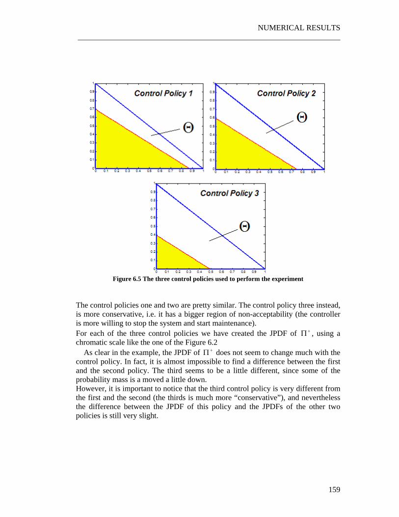
NUMERICAL RESULTS ___________________________________________________________________
159
Figure 6.5 The three control policies used to perform the experiment
The control policies one and two are pretty similar. The control policy three instead, is more conservative, i.e. it has a bigger region of non-acceptability (the controller is more willing to stop the system and start maintenance). For each of the three control policies we have created the JPDF of +Π , using a chromatic scale like the one of the Figure 6.2 As clear in the example, the JPDF of +Π does not seem to change much with the control policy. In fact, it is almost impossible to find a difference between the first and the second policy. The third seems to be a little different, since some of the probability mass is a moved a little down. However, it is important to notice that the third control policy is very different from the first and the second (the thirds is much more “conservative”), and nevertheless the difference between the JPDF of this policy and the JPDFs of the other two policies is still very slight.

CHAPTER 6 ___________________________________________________________________
160
On these grounds we can conclude that the control policy does not have a significant impact on the JPDF of the +Π . This does not mean that we will completely ignore the correlation between the JPDF of the +Π and the control policy, but for similar control policy it is not a bad approximation to consider the JPDF to be identical. We will show in a later section how this can be exploited to improve the performance of the algorithm.

NUMERICAL RESULTS ___________________________________________________________________
161
6.4 Exploiting the properties of the JPDF In the last chapter we have been able to explore some very interesting properties of the JPDF of the a posteriori vector. In this section we will try to explain how these properties could be used to improve the performance of the algorithm.
6.4.1 The Snake shape The snake shape is an important property of the JPDF of +Π : through this property we can be sure that most of the probability mass of the JPDF is concentrated around a specific curve in the space (the snake body) and that this curve does not change with the state and with the time. The main advantages of this amazing property are two:
1. It seriously simplifies the research of the optimal control policy 2. It makes it possible to believe that an approximated analytical solution to the
problem is possible As already said in different situations the optimal control policy is just a region of non-acceptability in the space. The main problem is to find what is this region. If we had no clue of how this region looks like it would be impossible to search it, since we should try to find the optimal region over a theoretically infinite number of ways to partition the space Ω . The snake shape, from this point of view, is extremely helpful. Since we know that most of the probability mass is concentrated in a specific region of the space, we only need to explore this region. A good approach would be the following. We may try to find a curve interpolating the random points generated during the first time step (when we have smaller dispersion of the point) with a an analytical function (polynomial, exponential, etc) thus finding the “core” structure of the snake. We will call this curve as “core curve”.
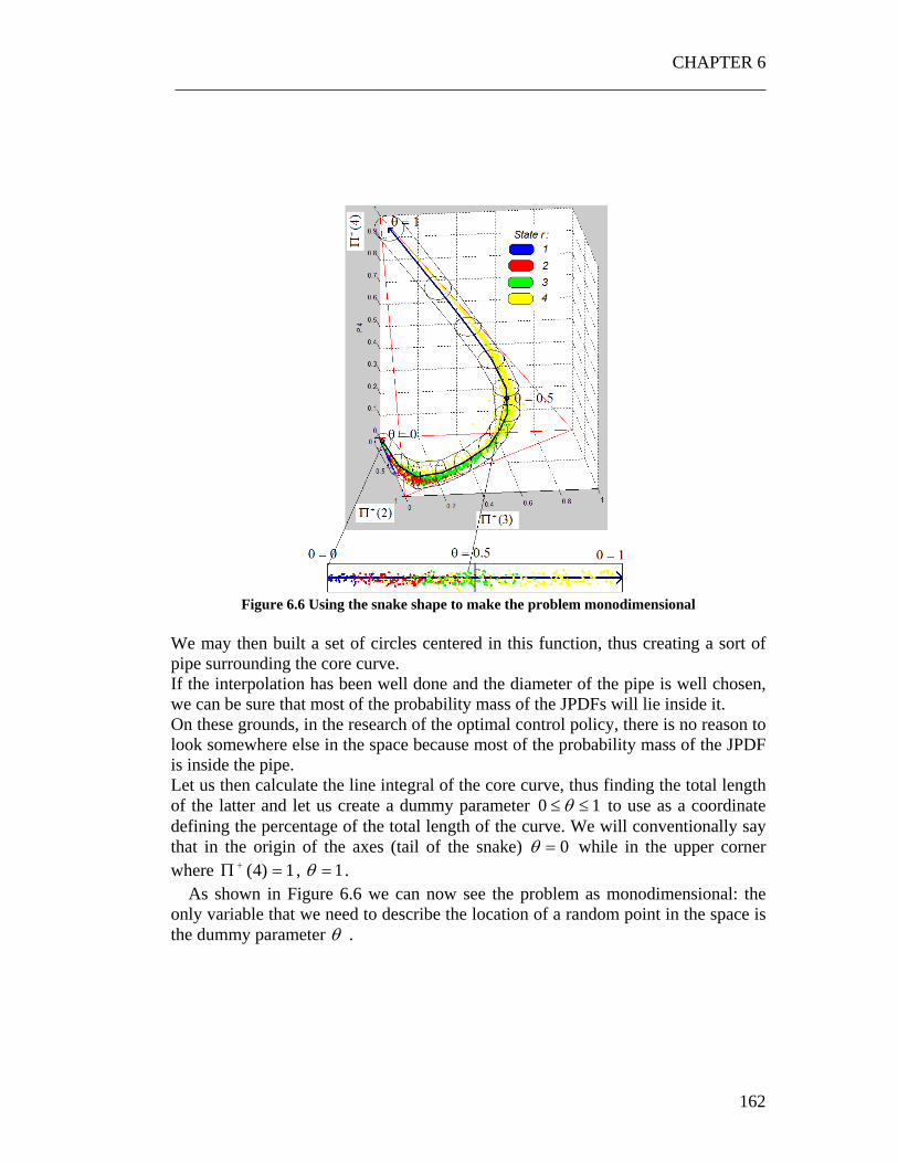
CHAPTER 6 ___________________________________________________________________
162
Figure 6.6 Using the snake shape to make the problem monodimensional
We may then built a set of circles centered in this function, thus creating a sort of pipe surrounding the core curve. If the interpolation has been well done and the diameter of the pipe is well chosen, we can be sure that most of the probability mass of the JPDFs will lie inside it. On these grounds, in the research of the optimal control policy, there is no reason to look somewhere else in the space because most of the probability mass of the JPDF is inside the pipe. Let us then calculate the line integral of the core curve, thus finding the total length of the latter and let us create a dummy parameter 10 ≤≤ θ to use as a coordinate defining the percentage of the total length of the curve. We will conventionally say that in the origin of the axes (tail of the snake) 0=θ while in the upper corner where 1)4( =Π + , 1=θ . As shown in Figure 6.6 we can now see the problem as monodimensional: the only variable that we need to describe the location of a random point in the space is the dummy parameter θ .

NUMERICAL RESULTS ___________________________________________________________________
163
We can thus see the JPDF of the +Π as a simple monodimensional probability density function, and we can find an optimal control policy based on the θ parameter: if optθπ >+ stop the system. This would make the problem extremely simpler because we would always be able to transform a generic K-dimensional problem in a simple monodimensional one.
6.4.2 Exploiting the weak dependence on the control policy The weak dependence of the JPDFs on the control policy is another extremely useful property that can be exploited to simplify the problem. In the original method that we have explained in Chapter 0, the Monte Carlo method has to be repeated each time a new control policy is explored. This would imply a significant increase in the computational burden of the algorithm since the Monte Carlo based research of the JPDFs is the most computationally intensive part of the model. This problem would basically remain the same even if we used a discretization based approach: in any case, the most computationally intensive part is always the research of the JPDFs. However, if we say that the JPDFs do not change much with the control policy, we are not forced to recalculated them each time a new control policy is explored. We can thus simply calculate it for once, and then explore a large set of new control policies using the same JPDFs. In other words, based on the same JPDFs, we would only have to perform the integral of this function over a new control policy non-acceptability region. The calculation of the integral, as already said, is absolutely trivial to perform (see Equation ( 5.28 )) and it requires a minimum computational time.

CHAPTER 6 ___________________________________________________________________
164
Figure 6.7 Exploiting the weak dependence of the JPDFs on the control policy. While in the Method 1 we are forced to recalculate the JPDFs for each new Control Policy, in the Method 2 we exploit the weak dependence property of the JPDFs. Instead of recalculating it each time, we store it and use it to explore new control policies.

NUMERICAL RESULTS ___________________________________________________________________
165
6.5 Properties of the p(n) functions In the last Chapters we have often talked about the )(np functions, which basically represent the core of the Controlled Case problem. They represent the probability that, if the system is in a state r at a time n, the controller may decide to stop the system and start maintenance. Using the Monte Carlo approach we are able to calculate them, and to have an idea of which is their shape.
We have done a set of experiments similar to the ones performed in the Section 6.1: we have take 3 different situations with different PDF of the quality of the parts. In particular, we changed the rate of overlapping of the distributions and checked how the probabilities )(np changed. The three situations are shown in the graphs in the next page:

CHAPTER 6 ___________________________________________________________________
166
Figure 6.8 The three situations which have been analyzed. There is a different rate of overlapping

NUMERICAL RESULTS ___________________________________________________________________
167
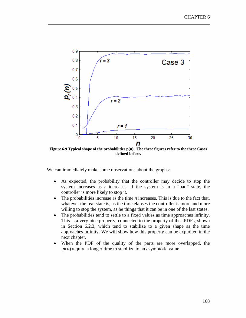
CHAPTER 6 ___________________________________________________________________
168
Figure 6.9 Typical shape of the probabilities p(n) . The three figures refer to the three Cases
defined before.
We can immediately make some observations about the graphs:
• As expected, the probability that the controller may decide to stop the system increases as r increases: if the system is in a “bad” state, the controller is more likely to stop it.
• The probabilities increase as the time n increases. This is due to the fact that, whatever the real state is, as the time elapses the controller is more and more willing to stop the system, as he things that it can be in one of the last states.
• The probabilities tend to settle to a fixed values as time approaches infinity. This is a very nice property, connected to the property of the JPDFs, shown in Section 6.2.3, which tend to stabilize to a given shape as the time approaches infinity. We will show how this property can be exploited in the next chapter.
• When the PDF of the quality of the parts are more overlapped, the )(np require a longer time to stabilize to an asymptotic value.
NUMERICAL RESULTS ___________________________________________________________________
169
6.5.1 Exploiting the properties of the p(n) functions The very nice thing underlined in the previous Subsection is that the probabilities
)(np , which are the nucleus of the algorithm for the research of the optimal control policy, have an extremely simple analytical structure. The first advantage is that, since those probabilities converge to an asymptotic value, it is not necessary to keep calculating them for WTLn ,..,1= but we can stop when the value of the )(npi has reasonably stabilized to a given values, i.e. when
ε≤−− )1()( npnp ii , with ε arbitrarily small. However, we can even beyond that. The simple shape of such probabilities makes it well possible to interpolate them with an analytical expression. On these grounds, the research of such probabilities can be narrowed down to the research of the set of parameters describing the analytical expression of those functions. We would therefore transform the problem of the research of each single value of )(npi to the (much simpler) problem of the research of a small set of parameters. The huge advantage of this alternative approach is that we could seriously reduce the number of iterations required by the Monte Carlo approach to calculate each value of the )(npi : in fact, we do not need a precise estimation of each of these values, but we look for a precise estimation of the parameters.
Chapter 7
Improvements, Future Developments and Conclusions 7
7.1 Improvements The model discussed in the previous pages is the first attempt to find Bayes-optimal control policies for deteriorating systems based on continuous measurements. The target of the document was so to find a complete solution to a relatively simple problem. However, a wide set of improvements can be applied to the method in order to consider more complex situations. In this subsection we will try to list some of them.
7.1.1 Extension to generically distributed duration of the deteriorating tool
One of the main assumptions of the basic model used in this paper is that the time to failure of the deteriorating tools are random variables distributed with a Pascal distribution. Such approximation has made possible to model the system with the line shaped Markov Chain showed in Figure 2.1. However, for a lot of real system this approximation may not be adequate, and so the results predicted with this method may not match real data. On these grounds a different way to model such systems would be necessary. As shown in the previous pages, the model developed in this paper is not sensitive to the type of Markov chain through which the system is modeled. Given a set of K working states, and given all the other necessary data, the method is able to find a cost optimal control policy for that system. So, if could model a given system with a

IMPROVEMENTS, FUTURE DEVELOPMENTS AND CONCLUSIONS ___________________________________________________________________
171
proper Markov Chain, the optimal control policy can always be found using the described method. A vast range of papers and research have been carried out to model specific probability density functions using a Markov Chain. One of the most recent and most powerful is [36], where a simple algorithm is developed to find the parameters of a Markov Chain that best fit a given probability density function. With Markov Chain smaller then 10 states, the authors show that it is possible to “interpolate” a very large set of common distribution. Using this alternative approach, it is possible to extend the developed method to a broader set of situation without incurring significant approximations.
7.1.2 Deterioration-dependent failures and maintenance time One of the starting assumption of the model was that the duration of the maintenance operations was independent of the state of deterioration of the system: when the controller decides to start maintenance, the expected duration of the latter is the same, regardless of the deterioration state of the system. However, this hypothesis is not always true: there are examples of maintenances whose duration depends on the deterioration state of the system. Take for example the cleaning of the internal surface of a pipe: the more the pipe is deteriorated, the longer it will take to take off the impurities from its internal surface. Another hypothesis done at the beginning of the paper is that the machine can “crash” only when it reaches the last operating state. This is not always true: in fact, a failure may occur at any level of deterioration. What is reasonable though is that the probability and perhaps the cost impact of a failure may increase as the deterioration increases. For the inner flexibility of the model, we can easily modify the Markov Chain of the deteriorating machine in order to consider such situations. A possibility is to connect each working state to a different maintenance and a different crash state: each of those states will have different durations and different costs. We may even consider the presence of different failure modes, introducing different types of crash characterized by different crash costs. Since the model is not affected by the type of Markov Chain through which the deterioration of the system is described, those modifications have little or no impact on the computational burden required to solve the problem.
CHAPTER 7 ___________________________________________________________________
172
7.1.3 Maintenance scheduling: proactive maintenance The optimal control policy defines the conditions for which it is cost optimal to stop the system and start maintenance. In many manufacturing environments, for organizational issues, maintenance operations can be performed more efficiently and quickly if scheduled beforehand. Therefore, it would be advantageous to have a model which is able to predict the expected time before the system will require maintenance with a reasonable level of precision. The model used in this paper can be perfectly used for this purpose: in fact, having the Markov Chain describing the deterioration dynamic of the system (initialized with the a posteriori probability vector) and the optimal control policy, it is not possible to find the expected value of this time, but also its probability distribution function (it is a discrete variable). On these grounds, precise statistical considerations can be applied to decide when it is time to start the “preparation” of the maintenance operations or to manage unexpected organizational issues. For example, if for tomorrow there is a strike of the maintenance operators in program and the probability that the system may require maintenance right tomorrow is relatively high, the plant managers may decide to start the maintenance operations by the end of the current working day. The same type of considerations can be used, for example, in the purchase and inventory management and of spare parts and for other organizational issues.
IMPROVEMENTS, FUTURE DEVELOPMENTS AND CONCLUSIONS ___________________________________________________________________
173
7.2 Future developments The stochastic model developed in this thesis is one of the first attempts to solve Partially Observable Markov Decision Processes describing maintenance problems, without using Dynamic Programming. The model is able to find the JPDFs of the a posteriori probability vectors, and thanks to the interesting properties of the model analyzed in the previous Chapter is able to address the problem of the research of the optimal control policy. The authors believe that this type of approach might be a first step towards a thread of Bayes-optimal models to solve maintenance problems which do not use Dynamic Programming. As explained, the pros of undertaking this alternative solution are many, and may lead to better and more accurate maintenance control policies. In theory, every model built in the past and solved using Dynamic Programming can be reformulated and solved using this different approach; the advantage is the possibility to consider continuous, non-windowed observations, which may lead to a more realistic and precise vision of the problems. Using a similitude with the traditional quality management approaches, this is like switching from the traditional Control Charts for Attributes to the Control Charts for Variables: as proved by years of research and practice in quality management, the charts for variables have led to better performances in many sectors. The model developed in this document can thus be seen as the “Chart for Variables” counterpart in the Bayesian methods for quality and maintenance management. As the Bayesian approaches to solve combined quality and maintenance management acquire more and more importance in the manufacturing systems design and management, using continuous observations could be an interesting direction of research for the future.

CHAPTER 7 ___________________________________________________________________
174
7.3 Conclusions In this document we have developed a method to find cost optimal maintenance control policies for a deteriorating machine based on the quality of the manufactured parts. The method considers all the most relevant costs associated to the maintenance management as well as their correlation, thus leading to an optimization of the global cost of the system. Besides the normal costs for performing maintenance and the induced loss in productivity due to the down times, the model considers the decrease in the quality of the manufactured goods (and its cost impact) due to deterioration of the system. Moreover, an increasing risk of failure is associated to higher deterioration levels of the machine, thus considering the safety costs, increase in maintenance costs and plant asset damage costs associated to such events. Coherently with some of the latest research threads on the topic, the quality of the manufactured parts is used as an essential information to take the decision (at each time step) as to whether to start maintenance or not. This is a typical Bayes-optimal method, in the sense that the maintenance decision is based on optimizing the expected cost of the system over a certain time horizon, given the information available. This type of approach is very useful in those situations where it is not possible or it is too expensive to inspect the machine (or a given deteriorating component in it) from the outside. In alternative, the quality of the manufactured parts can be used to get information, even if imperfect, about the state of the machine. This type of method is also reasonably cheap and has little impact on the system: while inspecting the deterioration state of a component requires additional devices installed on the machine, the quality of the manufactured parts is commonly measured on most of the manufacturing systems in order to separated good parts from scraps. On these grounds, information already available on the manufacturing floor would be used to support maintenance decisions. There are other existing researches using this same type of Bayesian approach. However, in all of them the Dynamic Programming (DP) is used to find the cost optimal decision given a finite time horizon. The major stumbling block of dynamic programming is to have to compute the one-step transition probability matrices of the Markov chain for every possible action of the decision-making process, and this makes the problem unsolvable (for computational reasons) unless seriously simplified. To that end, in past researches binary (or roughly discretized) measurements were considered as well as a windowing was applied on the latest observations.
IMPROVEMENTS, FUTURE DEVELOPMENTS AND CONCLUSIONS ___________________________________________________________________
175
The method developed in this paper does use the DP and so is not subject to these constraints. Every continuous (non-discretized) observation is used to recursively update the a posteriori vector, and the decision as to whether to start maintenance or not is based upon it. After proving that a single stationary optimal control policy based on the a posteriori vector exists and after showing that such policy has a fairly simple structure, we have built a method based on the Renewal Reward Theorem to evaluate the effect of a single control policy. The general analytical method, based on the iterative construction of the Joint Probability Density Functions (JPDF) of the a posteriori vector, has been solved numerically using a discretization or a Monte Carlo based approach. Given some important characteristics of the JPDFs (“snake shape” and independence of the control policy), a simple algorithm for the research of the optimal control policy has been proposed. Since the method is independent of the complexity of the Markov Chain, different types of systems can be modeled and more complex situations can be considered and solved using the same approach without incurring significant computational difficulties.
7.3.1 An example: the thermal spray coating nozzles deterioration problem.
In this subsection, a virtual application of the method is described. The purpose is to show an example of a situation where the application of the method would be possible and to list the set of steps necessary to implement it. The TSCM Inc. manufactures thermal spray coatings machines. Thermal Spray techniques are coating processes which involve spraying melted (or heated) materials onto a surface. The materials to be deposited as the coating are typically fed into a spray gun in powder or wire form where they are normally melted before being accelerated towards the substrate, or material to be coated (generally metal surfaces). As the sprayed particles hit the surface, they cool and build up into a laminar structure forming the thermal spray coating. The clients of the TSCM are companies manufacturing mechanical parts which need to be coated at some stage of the production process. The coating operations are performed by thermal coating stations, which are the most delicate and most expensive part of the process, and are commonly considered as the bottleneck of the

CHAPTER 7 ___________________________________________________________________
176
line. The roughness of the coating is a very important parameter and needs to be measured each time a part leaves one of the coating stations. If such parameter exceeds a given value, the parts has to be scrapped. While the other components of a thermal spray machine have usually long lives, nozzles are subject to severe rate of deterioration since the droplets of melted material tend to settle and solidify on the internal surface and on the border of the nozzle. As the nozzle becomes dirtier and dirtier, the spray gun does not work properly and the roughness of the coated surface tends to increase. Moreover, if the accumulation of material increases without control there is a risk that the nozzle may become clogged, thus generating a dangerous pressure increase in the combustion chamber, with possible failure of the whole thermal coating machine or other serious safety issues. On these grounds, a correct replacement policy of the nozzles is one of the main concerns of the production managers of those companies. Unfortunately, such type of policy is not easy to find. In fact, the deterioration of the nozzle depends on a wide range of external parameters which may facilitate the accumulation of clogging material (temperature, input materials, external conditions, etc) . To overcome this hurdle, the clients of TSCM used a type of periodic preventive maintenance policy: each nozzle was used for a pre-defined period of time and was then substituted. However, because of the high risk associated to a complete clogging, most of them were forced to use unreasonably small periods of replacement. This seriously incremented the production costs of those lines, because of the cost for buying new nozzles and for the impact that the downtimes required to change nozzles had on the productivity of the line. Deterioration based methods, as an alternative to the periodic maintenance policies were also explored; however, checking the deterioration state of the nozzles directly is impossible, since no type of measuring probe would resist the temperature and the pressure with which the thermal coating operates. An interesting alternative hypothesized by a technician of one of the plants was to infer the deterioration state of the nozzle from the (measured) roughness of the coated parts: even though there is not a unique analytical connection between roughness (which depends on a variety of factors) and deterioration, there is a strong correlation between these two factors. As a mean to improve the quality of the service offered to the clients TSCM decides to make an investment and develop an ad hoc maintenance service in order to minimize the economic impact of the nozzles replacement on the system of its clients. Aware of the extreme importance that the coating stations and their correct maintenance have on the system of their clients, TSCM decides to apply the latest

IMPROVEMENTS, FUTURE DEVELOPMENTS AND CONCLUSIONS ___________________________________________________________________
177
techniques of quality-based maintenance control policies in order to attain the maximum economic results. The model proposed in this thesis seems to perfectly fit with the type of problem analyzed in the last two pages, and we will suppose that TSCM decides to base its maintenance service on this model. To start, an experiment campaign has to be run in order to understand the dynamic of deterioration of the nozzles. To find robust results, TSCM decides to base its experiments on 5000 nozzles to be tested in the plant of one of its clients who decided to cooperate in the initiative. The nozzles are normally operated to coat test surfaces, and the roughness of each test surface is measured each time. The experiments are run following the elementary principles of the Design of Experiments techniques. After gathering enough data, the empirical distribution of the time to failure of the nozzles are built and the algorithm recalled in the Subsection 7.1.1 and shown in the paper [35] is used to find a Markov Chain able to “interpolate” such distributions. A scheme similar to the one shown in Figure 2.6 at page 29 is used to find the probability density functions of the quality of the parts associated to each operating state of the Markov Chain. Once the Markov Chain describing the system and the PDF of the quality of the parts are created, the deterioration dynamics of the nozzle can be perfectly described. Using this as an input, an optimal control policy is built for each client; in fact, while the deterioration of the nozzle is the same, the value of the manufactured products, the duration and the cost of the maintenance operations and the impact of the failures (crash cost) change among the different clients (each clients manufactures different products, have different maintenance organization and the downtime have different impacts). Using all these parameters as input of the model, optimal control policies are built for every client using the set of steps illustrated in Chapter 5. In order to actuate the established optimal control policy, a simple software using the information coming out of the station checking the roughness of the parts is installed. When the conditions to start maintenance are reached, the software will trigger a signal (acoustic, visual, etc) which tells the workforce to start the maintenance operations. Exploiting the knowledge of the deterioration dynamics of the system described in the Markov Chain of the latter, initialized with the current a posteriori probability vector, the software may also be able to evaluate (with a good level of precision) the probability that the system may require maintenance in a given period of time. Such information can be exploited to organize the maintenance operations

CHAPTER 7 ___________________________________________________________________
178
preventively, as described in Subsection 7.1.3, thus making the maintenance service more efficient.
REFERENCES ___________________________________________________________________
179
References [1] L. Furlanetto, M. Garetti, M. Macchi, Principi generali di gestione della
manutenzione, FrancoAngeli, Milano, 2006 [2] Edwards, D. J., G. D. Holt, and F. C. Harris (2000). A comparative analysis
between the multilayer perceptron neural network and multiple regression analysis for predicting construction plant maintenance costs. Journal of Quality in Maintenance Engineering 6(1), 45–60.
[3] Pierskalla, W. P. and J. A. Voelker (1973). A survey of maintenance models:
control and surveillance of deteriorating systems. Operations Research 21, 1071–1088.
[4] Araposthathis, A., V. S. Borkar, E. Fernandez-Gaucherand, M. K. Ghosh, and
S. I. Marcus (1993). Discrete-time controlled Markov processes with average cost criterion: a survey. SIAM Journal of Control and Optimization 31(2), 282–344.
[5] Jardine, A. K., D. Lin, and D. Banjevic (2006). A review on machinery
diagnostics and prognostics implementing condition-based maintenance. Mechanical Systems and Signal Processing 20, 1483– 1510.
[6] Martin, K. (1994). A review by discussion of condition monitoring and fault-
diagnosis in machine tools. International Journal of Machine Tools and Manufacture 34, 527–551.
[7] Nandi, S. and H. Toliyat (1999). Condition monitoring and fault diagnostic of
electrical machines: a review. In Thirty-Fourth IAS Annual Meeting, Volume 1, Phoenix, Arizona, pp. 197–204.
[8] Pusey, H. and M. Roemer (1999). Assessment of turbomachinery condition
monitoring and failure prognosis technology. Shock and Vibration Digest 31, 365–371
REFERENCES ___________________________________________________________________
180
[9] Wang, W., F. Ismail, and M. F. Golnaraghi (2001). Assessment of gear damage monitoring techniques using vibration measurements. Mechanical Systems and Signal Processing 15, 905–922.
[10] Wang, M., A. Vandermaar, and K. Srivastava (2002). Review of condition
assessment of power transformers in service. IEEE Electrical Insulation Magazine 18, 12–25.
[11] Saha, T. (2003). Review of modern diagnostic techniques for assessing
insulation condition in aged transformers. IEEE Transactions on Dielectrics and Electrical Insulation 10, 903–917.
[12] El-Shafei, A. and N. Rieger (2003). Automated diagnostics of rotating
machinery. In 2003 ASME Turbo Expo, Volume 4, Atlanta, Georgia, pp. 491–498.
[13] Tallam, R., S. Lee, G. Stone, G. Kliman, J. Yoo, T. Habetler, and R. Harley
(2003). A survey of methods for detection of stator related faults in induction machines. In Proceedings of the IEEE International Symposium on Diagnostics for Electric Machines, Power Electronics, and Drives, New York, pp. 35–46.
[14] Sabnavis, G., R. Kirk, M. Kasarda, and D. Quinn (2004). Cracked shaft
detection and diagnostics: a literature review. Shock and Vibration Digest 36, 287–296.
[15] Derman, C. (1962). On sequential decisions and Markov chains. Management
Science 9, 16–24. [16] Klein, M. (1962). Inspection-maintenance-replacement schedules under
Markovian deterioration. Management Science 9, 25–32. [17] Kolesar, P. J. (1966). Minimum cost replacement under Markovian
deterioration. Management Science 12, 694–706. [18] Luss, H. (1976). Maintenance policies when deterioration can be observed by
inspection. Operations Research 24(2), 359–366.

REFERENCES ___________________________________________________________________
181
[19] Smallwood, R. D. and E. J. Sondik (1973). The optimal control of partially observable Markov processes over a finite horizon. Operations Research 12(5), 1071–1088.
[20] E. J. Sondik. The Optimal Control of Partially Observable Markov Processes
Over the Infinite Horizon: Discounted Costs. Operations Research Vol. 26, No. 2 (Mar. - Apr., 1978), pp. 282-304
[21] Pat´e-Cornell, M., H. Lee, and G. Tagaras (1987). Warnings of malfunction:
the decision to inspect and maintain production processes on schedule or on demand. Management Science 33(10), 1277–1290.
[22] Tagaras, G. (1988). An integrated cost model for the joint optimization of
process control and maintenance. Journal of Operations Research Society 39(8), 757–766.
[23] Schick, I.C., G. Bertuglia, and S.B. Gershwin, Bayes-Optimal Reactive
and Proactive Maintenance Control Policy for a Deteriorating Machine, under revision (2006).
[24] Barlow, R. E., F. Proschan, and L. C. Hunter (1965). The mathematical theory
of reliability. NewYork: Wiley. [25] D. G. Nguyen, D. N. P. Murthy Optimal Preventive Maintenance Policies for
Repairable Systems. Operations Research, Vol. 29, No. 6 (Nov. - Dec., 1981), pp. 1181-1194.
[26] H. Pham, H. Wang, Imperfect Maintenance, European Journal of Operational
Research Volume 94, Issue 3, 8 November 1996 - Elsevier., Pages 425-438 [27] SH. Sheu, RH. Yeh, YB. Lin, MG. Juang, A Bayesian approach to an
adaptive preventive maintenance model. Reliability Engineering and System Safety, 2001.
[28] MP. Berg, The marginal cost analysis and its application to repair and
replacement policies. European Journal of Operational Research, 1995.
REFERENCES ___________________________________________________________________
182
[29] T. Dohi, N. Kaio, S. Osaki. On the optimal ordering policies in maintenance theory—survey and applications. Applied Stochastic Models and Data Analysis, 1998.
[30] JM. van Noortwijk. Optimal maintenance decisions on the basis of uncertain
failure probabilities. Maintenance Engng, 2000 - emeraldinsight.com [31] S. Dayanik, U. Gurler. An Adaptive Bayesian Replacement Policy with
Minimal Repair. Operations Research, 2002. [32] FA. Van der Duyn Schouten, CS. Tapiero. OR Models for Maintenance
Management and Quality Control. European Journal of Operational Research, 1995.
[33] A. Gosavi, TK Das, S. Sarkar. A simulation-based learning automata
framework for solving semi-Markov decision problems under long-run average reward. IIE Transactions, 2004
[34] R. Gallager, Discrete Stochastic Processes, Chapter 3. Kluwer Academic
Publisher, 1996 [35] E Fernández-Gaucherand, A Arapostathis, SI Marcus, On the average cost
optimality equation and the structure of optimal policies for partially observable Markov decision processes. Annals of Operations Research, 1991
[36] A.Bobbio, A.Horvàrt, M.Scarpa, M.Telek, Acyclic discrete phase type
distributions: properties and parameter estimation algorithm. Oct 2002