policy reform, shadow prices, and market prices …personal.lse.ac.uk/sternn/058nhs.pdf · policy...

Journal of Public Economics 42 (1990) 145. North-Holland

POLICY REFORM, SHADOW PRICES, AND MARKET PRICES

Jean DRfiZE and Nicholas STERN*

London School of Economics, Houghton Street, London WCZA 2AE, UK

Received April 1989, revised version received February 1990

How should public projects and policy reforms be assessed when market prices give misleading signals? Revenues and costs at market prices then give distorted measures of social gains and losses and our appraisal should use social opportunity costs or ‘shadow prices’. We show how shadow prices may be integrated into an analysis of policy reform, demonstrate the critical dependence of these prices on government policy and analyse their relations with market prices. The model allows for a wide range of sources of impairment of price signals. We also discuss key issues in the analysis of price reform and ‘privatisation’.

1. Introduction

1.1. The objectives of the paper

Economists are often asked to give policy advice in situations where, it is claimed, prices give distorted or misleading signals. And many of them are fond of suggesting that governments should leave more to the market so that private agents can respond effectively to price incentives. While these positions are not necessarily contradictory, their juxtaposition should lead us to ask some questions. What do we mean by misleading signals? Can we define satisfactorily an index of scarcity or value which is not misleading? How do we identify the social opportunity cost or shadow price of a commodity? How do these shadow prices compare with market prices and under what circumstances will they coincide? Should governments leave

*This paper was partly written during a visit by Stern to the Fiscal Affairs Department (FAD) of the International Monetary Fund in July and August 1987. He is grateful to FAD and its Director, Vito Tanzi, for the invitation and hospitality. Support from the Suntory-Toyota International Centre for Economics and Related Disciplines and from the ESRC Programme on Taxation, Incentives and the Distribution of Income is gratefully acknowledged. We have been strongly influenced by the work of Roger Guesnerie on second-best theory. For helpful discussion and comments, we would also like to thank Tony Atkinson, Lans Bovenberg, Angus Deaton, Peter Diamond, Peter Heller, Mervyn King, Partho Shome, Richard Stern, Alan Tait, Vito Tanzi and two referees. The paper draws on our 1987 survey [Drize and Stern (1987)], which is more technical and may be consulted by the reader who wishes to pursue the subject in greater depth.

OQ47-2727/90/$3.50 0 1990, Elsevier Science Publishers B.V. (North-Holland)

2 J. DrPze and N. Stern, Policy reform and market prices

decisions to the market when prices give impaired signals? How can the government improve price, tax, or regulatory incentives? How can concern with income distribution be integrated systematically with measures to improve efficiency? Generally, how can shadow prices and market prices be combined in the understanding and implementation of the reform of government policies?

The purpose of this paper is to suggest a framework for the analysis of these issues and to provide the practitioner with a structured and productive way of thinking about the problems of how market distortions should influence proposals for reform. In so doing we attempt to provide help in identifying the empirical questions that should be raised and the judgements that need to be made before deciding on a particular line of policy.

We shall begin the analysis (in section 2) by defining shadow prices. We shall argue that there is only one sensible way to approach the definition of shadow prices if those shadow prices are to be used to evaluate the net impact on welfare of public sector projects. The shadow prices are the social opportunity costs of the resources used (and correspondingly for outputs generated). Having defined shadow prices in this rather general way, we then set out a formal exposition of their properties in a model of an economy where markets need not be perfectly competitive. Such models are generally more difficult to analyse than those with well-functioning competitive markets, but we shall try to make the discussion accessible and avoid unnecessary technicalities. The literature on shadow prices has been somewhat bewildering in its different definitions, methods, and models, and we shall attempt to provide a unified analysis within which many of the apparently disparate results and propositions can be understood. The theory and discussion are microeconomic in form but a macro economy is, of course, implied. We make the link explicit in section 3 where we focus on

government revenue and the macro economy. Shadow prices are detined for public sector projects but they are readily

extended to the private sector. This extension is provided in section 4 where we also bring out relationships between shadow and market prices and show how the ideas of the paper can be applied to problems concerning efficiency of supply including privatisation and price reform. In this last application we provide some new results concerning basic questions of market reform which appear to have received insufficient analytic attention. Given current concerns for the reform of socialist econo,;iies the particular question of when one should raise the price of a good in e xcess demand (or lower price for excess supply) is of special interest. A summary and concluding comments are provided in section 5.

The paper is mainly expositional. We attempt to present a way of thinking coherently about policy reform in second-best economies, without pretending to supply general formulae that can blindly be applied to specific problems.

J. D&e and N. Stern, Policy reform and market prices 3

The formulation and many of the results draw on our earlier, more detailed and technical survey [Dreze and Stern (1987)]. The interested reader is referred to that survey for a more comprehensive and rigorous discussion.

1.2. The motivation for using shadow prices

In the remainder of this section we shall review briefly the lessons of the standard theory of prices and policy for competitive economies and then identify some complications that may invalidate the use of prices as indicators of social opportunity costs or values. This will help to explain our choice of model for section 2 and indicate which types of complication are

considered and which are not. It is convenient to approach the discussion of the social value of

commodities in distorted economies by defining an undistorted system where shadow prices would coincide with market prices. A ‘distorted economy’ is defined here as one where market prices and shadow prices do not coincide. This reflects our concern with distortions in (price) signals, rather than with deviations in economic organization from some allegedly ‘undistorted’ or ‘perfect’ system (such as that of competitive markets). Two further remarks are necessary. First, a competitive economy may well be ‘distorted’ in this sense, e.g. if the distribution of income fails to be optimum (see below). Second, there is no general presumption that price distortions, as defined here, should be systematically removed, in the sense that market prices and shadow prices should be brought as close as possible to each other (see subsection 4.4). Whether they should be removed or not depends, in fact, on the kind of policy tools that are available for this purpose.

It is a well-known result of classical welfare economics that under standard conditions (particularly the presence of all markets and the absence of externalities), a perfectly competitive equilibrium is Pareto efficient. In order for market prices to reflect the social value of commodities, the distribution of income should also be optimum according to the ethical judgements underlying the shadow price system. This additional requirement is often swept under the carpet, but this attitude is really hard to defend. Indeed, it is arguable that an essential role of government is to ensure that the standard of living of poorer groups receives some protection. Many would go further than this; indeed, redistribution is a commonly articulated concern of (and demand on) governments. Incorporating this objective typically requires sustained attention to the distributional consequences of government policies. To achieve an optimum distribution of income without interfering with the price system one needs to be able to redistribute resources and raise government revenue by lump-sum taxes and transfers (i.e. taxes and transfers which cannot be altered through the behaviour of agents). Since appropriate fiscal instruments of this kind are typically not available, shadow prices are

4 J. Drhze and N. Stern, Policy reform and market prices

liable to deviate substantially from market prices even in perfectly competitive economies.

Further distortions arise when the economy does not have the necessary features for Pareto efficiency described above. Possible sources of interference with the marginal equalities which are necessary for efficient allocation include: (i) indirect or income taxes; (ii) uncorrected externalities; (iii) quantity controls; (iv) controlled prices; (v) tariffs and trade controls; (vi) oligopoly; and (vii) imperfect information, transaction costs, and missing markets. The first five of these sources of imperfection are either included in whole or in part in the models that follow or can be easily added. The last two are more problematic.

2. The basic theory

We want to derive a set of shadow prices reflecting the social value of commodities, in order to guide policy reform and the choice of public sector projects. To this end, the shadow price of a commodity is defined as its social opportunity cost, i.e. the net loss (gain) asssociated with having one unit less (more) of it. The losses and gains involved have to be assessed in terms of a well-defined criterion or objective, which is referred to as ‘social welfare’. The evaluation of social welfare is naturally based (at least partly) on assessments of the well-being of individual households, supplemented by interpersonal comparisons of well-being. The latter are embodied in what we shall call ‘welfare weights’. This is not the place to debate which weights should be used - they should be discussed responsibly and intelligently but are ultimately value judgements depending, inter alia, on one’s views of inequality and poverty.

It is difficult, however, to dispense with the reliance on the notion of social welfare. Most practical examples of policy reform or public projects make some people better off and some worse off and we have to take a decision which trades off these gains and losses. Implicitly or explicitly we shall be using weights. In our judgement, attempts to produce cost-benefit tests for policy appraisal that avoid interpersonal comparisons have not got very far. For example, hypothetical transfers of the Hicks-Kaldor variety that could yield Pareto improvements are not relevant when such transfers will not take place; and if such transfers do take place systematically it is straightforward to incorporate them in the present framework. Also, assertions that ‘a dollar is a dollar is a dollar’ - that money values across households can be simply added up - do not avoid value judgements but invoke a specific one which says that all welfare weights (in terms of social marginal utilities of income) are equal. This is not an ethical position we would find attractive and, like other ethical statements, it would require explanation and discussion rather


than a simple assertion. Furthermore, it risks serious logical inconsistencies

[see, for example, Roberts (1980)]. In this paper we shall make extensive use of the Bergson-Samuelson social

welfare function. This amounts, in effect, to assuming that (1) individual well- being depends only on the fixed characteristics of individuals and on their consumption of commodities (so that social welfare can be defined on the commodity space), and (2) the marginal rate of substitution between two commodities going to the same individual are the same in the social welfare function and in the individual ‘utility function’ [see Dreze and Stern (1987) for further discussion and note that, to keep things simple, we are excluding externalities]. We shall not be constrained to any particular form of the social welfare function (the choice of which would involve additional assumptions and arguments) but shall present results in relation to a general function of the Bergson-Samuelson variety. Much of the theory would go through with a more general social objective although a number of the results which link social welfare to market choices would have to be modified.

When the social opportunity cost or shadow price of a good is defined in terms of the marginal effect on social welfare of the availability of an extra unit, it leads directly to a ‘cost-benefit test’, i.e. projects which make positive profits at shadow prices should be accepted because they increase welfare. Indeed, it should be clear (and see below) that no other definition of a shadow price can have this property. Thus, in this paper there will be one single definition of shadow price - it is the increase in social welfare resulting from the availability of an extra unit of the specified commodity. Strictly speaking, one also has (generally) to state from which agent the extra unit comes. For specificity, and because the interest here is primarily in public sector decisions, this agent will be understood to be the public sector. The shadow prices themselves will depend on the social welfare function and on how the economy, including the government, functions. But there is nevertheless essentially only one definition of the concept which allows their systematic link to cost-benefit tests.

In subsection 2.1 we provide a formal definition of shadow prices and illustrate the basic ideas with simple examples. The model we shall use is set out and discussed in subsection 2.2, and in subsection 2.3 we describe the relationship between optimum policies, shadow prices, and policy reform. Guidelines for reforming policy, and the rules satisfied by shadow prices, are analysed in subsection 2.4.

2.1. Definitions and simple examples

Our definition of shadow prices requires us to calculate the effect of an extra unit of net public supplies (the latter are represented by the vector z)

6 J. Dr&e and N. Stern, Policy reform and market prices

on social welfare. The public supplies are to be interpreted as outputs of and (negative) inputs in public production, rather than as public consumption (or what is conventionally termed ‘public goods’). Thus, they do not impinge directly on social welfare but only affect it through the variables that influence household welfare and demands: prices, wages, rations, and so on.’ We shall think of these variables as being of two types: ‘control variables’, s, and parameters or ‘predetermined variables’, o. The former are determined within the system, subject to the scarcity constraints that usages of goods cannot exceed availability, and to any other constraints that may be relevant. The variables o are fixed as parameters of the system. We shall, however, examine the consequences of shifts in these parameters.

We shall refer to the person or agency responsible for the evaluation of public decisions as the ‘planner’. This does not imply that we think of the government as a well-tuned, harmonised whole, acting coherently and consistently in pursuit of a well-defined set of objectives, captured by a single social welfare function. The planner will usually be operating in a particular agency and may have to treat the responses of other government agencies (e.g. taxes set by the finance ministry or quotas specified by a trade ministry) as outside its control. This causes no problems for the analysis since such items can be included among the list of predetermined variables, o. We shall assume that the planner chooses those variables which are in its control with respect to the same social welfare or objective function that is being used to evaluate changes in public supplies. This is simply an assumption of consistency for the planner in the selection of those variables which are within the range of control (and this basic consistency is indeed what the adviser may recommend). The planner’s range of control may, however, be so limited that there is essentially no choice at all. Crudely, there may be exactly the same number of constraints as there are control variables. This is the approach typically adopted in cost-benefit theory and practice. It does not disturb the analysis and is retained as an important special case throughout. We shall refer to this case as one where the model is ‘fully determined’. Our analysis represents therefore a generalisation of the standard approach.

The problem then is one of an optimising planner, but where that planner may have little (or negligible) scope in the selection of policies. The planner may well be asked, however, to decide on, or appraise, new opportunities in the form of new (small) projects, dz, or in the form of marginal reforms, or shifts, do, in variables which were initially regarded as predetermined.

‘Household welfare depends on individual consumption and not on aggregate supplies as such, and the link between consumption and supplies will be provided by the scarcity constraints of the model. Public goods and, more generally, externalities can be included in the model in a straightforward way although they will not be a central concern in what follows.

J. D&e and N. Stern, Policy reform and market prices I

It is important to note here that our list of ‘control variables’ includes what one may wish to call the ‘endogenous variables’ of the system, i.e. the variables whose value is determined by the constraints of the problem. To put it crudely again, when there are I constraints, a vector of K control variables can often be interpreted as consisting of I ‘endogenous variables’, and (K-I) variables under the effective and direct control of the planner. We shall, however, want to consider all K variables together, and the distinction between endogenous variables and control variables will often be somewhat arbitrary. For instance, in a model where the only constraints are the scarcity constraints and the control variables consist of prices and indirect taxes, it does not matter whether we choose to describe prices as being determined by the market-clearing process and taxes by the planner, or the other way round. From a formal point of view, it is enough to note that both prices and taxes should be treated as ‘control variables’, given that the scarcity constraints enter the model explicitly. This point is important for a correct interpretation of the models analysed in this paper.

We are now in a position to define shadow prices. We write social welfare V(s;w) as a function of s and ao, and think of the ‘planner’s problem’ as that of choosing s to solve

maximise V(s; w) subject to E(s; o) - z = 0, (2.1)

where E(s;o) is the vector of net demands arising from the private sector, z is (as indicated earlier) the vector of net supplies from the public sector, and 0 is a vector of zeros. The constraints expressed by (2.1) are the scarcity constraints, which say that available supplies must match demands. There may in practice be additional constraints. Often it will be possible to capture these constraints by considering some variables as predetermined, and to this extent they are included in our formulation; but where they cannot be modelled in this way they should be included as constraints additional to the scarcity constraints. To keep things simple, we shall avoid including them in the analysis that follows [see Dreze and Stern (1987) for a more general treatment].

Given z and o, the solution of (2.1) gives a level of social welfare which we write as V*(z;o) - the maximum level of social welfare associated with the production plan z (given 0). The shadow price vi of the ith good is defined

by

vi = w*/3z,. (2.2)

Thus, vi is precisely the increase in social welfare associated with a unit marginal increase in zi; or the social opportunity cost in terms of social welfare of a marginal unit reduction in zi. Alternatively, relative shadow


prices represent marginal rates of substitution in the social utility function V*(.) defined on the space of commodities.

A project is a small change in public supplies, dz (private projects are discussed in section 4). We can see from eq. (2.2) that the value of a project dz at shadow prices, vdz (i.e. xividzi), is equal to dV*, so a project increases social welfare if and only if it makes a profit at shadow prices. Thus, the cost-benefit test ‘accept the project if it is profitable at shadow prices’ correctly identifies all those projects that are desirable in the sense of increasing social welfare.2 Our definition of shadow prices is, of course, designed with precisely this property in view, and it can be seen that any set of relative prices that fails to coincide with the relative shadow prices defined by eq. (2.2) cannot possess the same property. Notice, on the other hand, that it is only relative shadow prices that matter and we can always scale the vector v up or down by a positive factor without changing anything of substance. We have not assumed that public production has been chosen optimally. This is, of course, retained as a special case since the analysis can be applied at any z. The planner, however, might be unaware of the detail of production possibilities and therefore unable to go straight to the best point in the production possibility set. Indeed, the role of shadow prices is precisely to evaluate those production possibilities of which he becomes aware. Finally, it must be stressed that the shadow prices discussed in this paper are appropriate only for the evaluation of small projects: for large changes, differential techniques based exclusively on first-order terms are no longer adequate.3

The change in welfare from an extra unit of public supplies comes about through the resultant changes in the variables which affect household welfare. These changes will, of course, be determined by the structure of the economy including, in particular, the policy instruments available to the government.4 The link between shadow prices and the tools at the government’s disposal may be illustrated using two simple examples.

Consider an economy with a single consumer who supplies labour to produce corn. The only firm is owned entirely by the government. In the first

‘Strictly speaking, if a project makes exactly zero profit at shadow prices, one should examine second-order terms to see whether it is socially desirable or not. If vdz is zero, then the change in welfare to second-order is dz’Adz, where A is the matrix of second derivatives of V* with respect to z.

%ee, for example, Hammond (1983) for a discussion of the problems raised by the analysis of large projects.

4Notice that the project will generally imply some changes in policy instruments and it is clear, and illustrated in what follows, that the form of adjustment will be critical to the welfare implications of the project. However, some projects may be directly linked to changes to parameters in the vector w. For example, a foreign donor might link support for a project to a change in a quota. In this case we should appraise the project by considering the welfare effects of (dz,do). This would be given by vdz+(aV*/aw)dw. We discuss (aV*/ao) in the next subsection; see, in particular, eqs. (2.11) and (2.12).

.I. D&e and N. Stern, Policy reform and market prices 9

example the government can control the economy fully in the sense that it can allocate labour and corn in both production and consumption subject only to the availability of each good. The control variables are the quantities of corn and labour in both production and consumption. In the second example the government has to work through the price system and can only obtain labour by hiring at each wage the amount the worker-consumer wishes to supply at that wage. Furthermore, it cannot levy lump-sum taxes, i.e. a poll tax or subsidy is ruled out. It is clear that in the second case the powers of the government are more limited than in the first and that the overall level of welfare it can achieve will be lower. It is also true that the marginal rates of substitution in terms of social welfare, or relative shadow

prices, will be different in the two cases. The problem is illustrated in figs. 1 and 2. In the first case (fig. 1) the

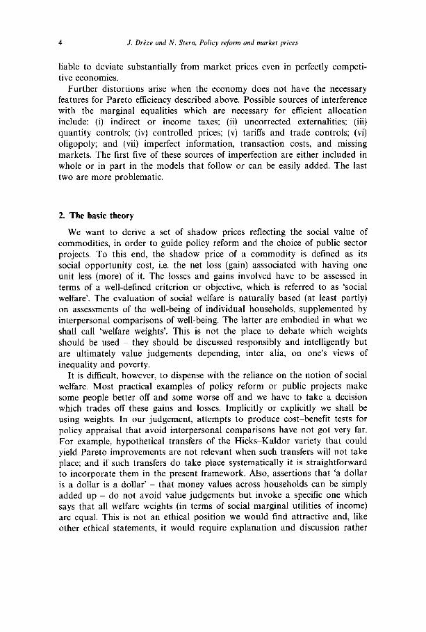
government has complete control over the economy and chooses the lirst- best allocation, X. The relative shadow prices are given by the loss of labour (i.e. extra labour required of the worker) that would hold social welfare constant if an extra unit of corn became available. The changes envisaged in response to the increased availability of a unit of corn must be achievable making the best possible use of the tools at the government’s disposal and observing the scarcity contraints. If an extra unit of corn becomes available, then utility could be held constant by a marginal increase in labour from X along the line DE towards D. The gradient of the line DE gives the marginal rate of substitution in social welfare and hence relative shadow prices.

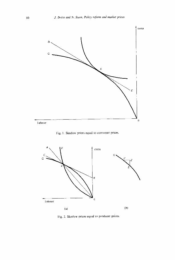
In the second case the government can choose only points along the offer curve OF in fig. 2(a). Since utility increases as we move up the offer curve (higher real wages) the optimum will be at Z where the offer curve cuts the production frontier OG. Relative consumer prices (the real wage to the consumer) are represented by the gradient of the line OZA and the marginal rate of transformation in production (the marginal product of labour here) is given by the gradient of BC. Thus, marginal rates of substitution for the consumer and marginal rates of transformation for the producer are not equal. The former is equal to the consumer price ratio and we may think of the latter as the producer price ratio. The difference is a tax, or if it is negative, a subsidy. Here it is a subsidy that is financed by the profits of the firm (at the given producer price ratio) of OB in terms of corn. If we now have an extra unit of corn, what will be the increase in labour requirement which will maintain utility constant given the tools at the government’s disposal, i.e. when we are restricted to movements along the offer curve? It is clear that constant utility must involve a return to Z since any other point on the offer curve involves higher or lower utility. Thus, the consumer price ratio must remain unchanged after the adjustment and the accommodation to the changes must be on the production side. This means that the change in labour in response to an extra unit of corn must be one that takes us back

IO J. Drdze and N. Stern, Policy reform and market prices

Fig. 1. Shadow prices equal to consumer prices.

C G

G

r z’

\

Z

labour 0

(a) (b)

Fig. 2. Shadow prices equal to producer prices.

.I. Drkze and N. Stern, Policy reform and market prices 11

to the production frontier so that production can adjust to take us back to

Z. The increase in availability of one unit is represented in fig. 2(b) by the move to Z’ and the increase in labour to regain the frontier by the move Z’ to Z”. Production can then be adjusted to bring us back to Z with no utility change. The marginal rate of substitution in social welfare is now seen to be given by the gradient of BC or relative producer prices.

It is straightforward to generalise these results to higher dimensions and several consumers, and some related results are discussed below. These simple examples, however, illustrate the important point that shadow prices depend on the tools at the government’s disposal: we have seen that there will be cases where they are equal to consumer prices and others where they are equal to producer prices. We are also going to find examples where they are averages of the two, or obey more complicated formulae.

2.2. The model

We shall now set out the basic model in which the properties of shadow prices will be investigated. This model is, in effect, a mixture of fix-price and flex-price models (in the language of Hicks) where prices in some markets are free to adjust but in others are not. Households and firms are price takers, but may be subject to quantity rationing in certain markets. This formulation will allow us to capture at once the important phenomena of price responses as well as quantity rationing. In particular, the familiar themes of the literature on temporary equilibrium with quantity rationing, such as Keynesian unemployment, are firmly within our framework.

We have H consumers (indexed by h = 1,. . , H), one private firm and one public firm. It is straightforward to extend the model to allow for an arbitrary number of private and joint public-private firms [see Dreze and Stern (1987)], but we are trying to keep the model as simple as possible whilst retaining its essential features. In a similar spirit we shall ignore

externalities. There are I goods, indexed by i= 1,. . . , I (distinguished, if necessary, by time and contingency). The private firm trades at prices given by the vector p and its net supply vector is y. We follow the usual convention that a negative supply by a firm represents a demand for an input and a negative demand by a household represents a supply by that household. The firm may be subject to quantity constraints on its choice of inputs or outputs. There are represented by an I vector of lower bounds j_ and a similar vector of upper bounds jj+; the 21 vector (y-, y+) is called 7. When the firm has maximised profits subject to the constraints it faces, its output of the ith good will be equal to the ith component of j- or of y+, or will lie between them. If it is equal to either the lower bound or the upper bound we say that the corresponding bound is the ‘binding constraint’. The binding constraint for good i, if any, is referred to as pi (the upper and lower

12 J. D&e and N. Stern, Policy reform and market prices

bounds cannot both be binding unless they are equal). The firm’s prolit- maximising supply y(p, y) is then a function of the prices and quotas which it faces. Its pretax profits, n(p,jj)), are also a function of p and J and are distributed to households according to the shares Oh. We denote 1 -Ch Oh by i, which represents the government’s share in the profits of the private firm, including any profits tax.

Households face prices 4 =p+ t, where t is the vector of indirect taxes (linear factor taxes are included within the components of t but there are no taxes on intermediate transactions). The hth household receives lump-sum income mh=rh+ Ohn, where rh is a lump-sum transfer from the government (positive, zero, or negative). Each household chooses a utility-maximising consumption vector X* subject to its budget constraint and quantity constraints which are represented by vectors of quotas, Xh,X’!+, as with the firm. We denote the 21 vector (Xh,X’!+) by Xh and the relevant binding constraints by $. The demands xh of household h are functions of q, Xh, and mh. They are written as xh(q, Xh, mh), but the identities q-p + t and mh= rh + eh7c should be kept in mind throughout.

The vector of net government supplies is z as before, and the vector of net imports is denoted by n. There is a given endowment F of foreign exchange, and world prices are fixed at p’“. F has an analogous status to z in the analysis in that it is exogenous to the optimisation but will be amongst those variables for which exogenous shifts will be examined. The scarcity constraints are then

Txh-y-n-z=O, (2.3)

p”n-F=O. (2.4)

We have chosen to write (2.4) separately from (2.3) to bring out the role of foreign trade more sharply. A more unified treatment, dispensing with (2.4), can be obtained by treating foreign exchange as a separate commodity and net imports as the net supplies of a separate firm. However, for greater transparency we shall treat foreign exchange and net imports explicitly.

The constraints are written as equality constraints without loss of generality, since they simply trace what happens to each unit of each commodity - disposal activities (with or without cost) could be included in a straightforward way [see Dreze and Stern (1987) for details]. To keep things simple we have supposed that the only constraints which arise are the scarcity constraints (2.3) and (2.4) and those which can be expressed in the form that a variable is ‘predetermined.

The vector s of control variables consists of K variables drawn from the following list:

.I. Drhe and N. Stern, Policy reform and market prices 13

(Pi), lti)9 trh)9 (xf)~ (Yi), Ceh)9 tni)3 (2.5)

where i=1,2 ,..., I,and h=l,2 ,..., H. The variables included in s are under the planner’s control, but they must

be chosen subject to the constraints (2.3) and (2.4). The more variables s contains, the larger the degree of freedom for the planner. Crudely speaking, if there are just (I+ 1) control variables, then the planner has no real choice since (2.3) and (2.4) represent (I + 1) constraints - this is the ‘fully determined’ case to which we have already referred. If there are more than (I+ 1) variables in the list s, then the planner has a genuine choice which it exercises so as to maximise social welfare. The variables in (2.5) which are not in s are predetermined, or are parameters, and denoted as before by o.

Finally, the social welfare function takes the Bergson-Samuelson form W(u’, U2, . . . ) uH), where uh is the level of utility of the hth household. This can also be written as

V(s; w) E W(. . . ) uh(q, Xh, rnh), . . . ,), (2.6)

where uh is the indirect utility function relating individual welfare to prices, rations, and income.

In the remainder of this paper we shall assume some familiarity with the elementary properties of the functions xh(q, Xh, mh), y(p, j), vh(q, Xh, mh), and 7t(p,y), i.e. with the basic theory of competitive demand and supply in the presence of quantity constraints or rationing. We also assume knowledge of simple optimisation techniques using Lagrange multipliers.

2.3. Optimum policies, shadow prices, and policy reform

Nearly all our results are derived from the first-order conditions for the maximisation of social welfare subject to the scarcity constraints (2.3) and (2.4). We shall examine, in particular, the Lagrange multipliers associated with the scarcity constraints. It should be clear that this is a natural way to proceed since these Lagrange multipliers will tell us precisely how much social welfare goes up if we have a little extra of public supply, and this corresponds exactly to our definition of shadow prices. To see this, let us write the Lagrangian L of the social welfare maximisation problem as

(2.7a)

where p is a Lagrange multiplier on the foreign exchange constraint, A a vector of Lagrange multipliers on the other scarcity constraints, and

E(s;w)rCxh-y-n. h

(2.7b)


Now let V*(z,F;o) denote, as before, the maximum social welfare associated with given values of z, F, and w. A standard result of optimisation theory (the ‘envelope theorem’) states that the gradient of the ‘maximum value function’, V*, is identical to the gradient of the Lagrangian, L. Therefore we have

(2.8a)

which confirms our assertion that the Lagrange multipliers on the scarcity constraints can be interpreted as ‘shadow prices’ in the sense defined earlier.5 Similarly we can at once derive

av*_aL aF aF-p’

(2.8b)

so that ,u can be interpreted as the marginal social value of foreign exchange: it measures the increase in social welfare resulting from the availability of an extra unit of foreign exchange. Notice that the shift in V* following a change in z works through the effect of a change in s on household utilities. However, the shift in L is at constant s [see the arguments of L in (2.7a); we can ignore any effects operating on L through s precisely because s has been chosen optimally - this is the ‘envelope property’].

Our writing of (2.3) and (2.4) separately to replace the constraint in (2.1) means that the evaluation of a project (dz,dF) is now given by whether or

~ Vidzi+C1dF>O, i=l

(2.9)

where we accept the project if (2.9) holds. Note that the foreign exchange

not

component, dF, will be zero unless the project is tied to a direct gift of foreign exchange: the (direct and indirect) effects of a project on foreign exchange will be captured by the first term in the left-hand side of (2.9), and should not be counted again through the component dF.

As we have already pointed out, it is only the relative shadow prices in the

‘Notice that there are, generally speaking, many equivalent ways of expressing a set of constraints in an optimisation problem. In this context, rewriting the constraints in an equivalent manner would change the Lagrange multipliers but not the shadow prices. Thus, it is important to recognise that our definition of shadow prices comes first, and we have shown that they happen to be equal to Lagrange multipliers if the constraints on the problem are written in an appropriate way.

J. D&e and N. Stern, Policy xform and market prices 15

vector (vi, v2,. . . , v,,p) that matter. In other words, we are free to choose a unit of account for our shadow prices. One common practice in the literature has been to do the accounting in terms of foreign exchange so that p is set equal to one [see Little and Mirrlees (1974)].

The control variables are chosen to maximise social welfare subject to the scarcity constraints. The first-order conditions for maximisation are

i3L c?v _viiE=O zs,- as, as, )

(2.10)

if the kth control variable is any element in the list (2.5) excluding n,. The first-order conditions for ni are discussed below. The conditions (2.10) have a very natural interpretation: they tell us that at an optimum the direct effect on social welfare of a marginal adjustment in any control variable should equal the marginal social cost of the extra net demands generated. Thus, the shadow prices are picking up the welfare effects of the full general equilibrium adjustments in the system. In this sense they are sufficient statistics for the general equilibrium responses: they summa-<se what we need to know about those consequences for the purpose of policy evaluation.

The first-order conditions (2.10), together with those for net imports, n,, where relevant, give us a set of K first-order conditions, where K is the number of control variables. These K conditions, together with the (I + 1) scarcity constraints (2.3) and (2.4), determine the values of the K control variables, sk, at the optimum and the (I+ 1) shadow prices. Thus, we can see that to speak of ‘rules determining shadow prices’ and ‘rules determining optimum policies’ is to describe the same set or a subset of the same set of conditions but from a different viewpoint. Moreover, we retain the ‘fully determined’ case, with K =(I+ l), as a special case - here the scarcity constraints uniquely determine the controls and the condition (2.10) represents a set of equations which we must solve for the shadow prices given these values of the controls.

As we have already emphasised, when K is greater than (I+ 1) one could think of a particular subset of control variables, K -(I + 1) in number, as the variables directly under the control of the planner, and the remaining (I + 1) as determined endogenously from the general equilibrium system. This dichotomy may occasionally be helpful in interpretation and to fix ideas but, analytically, it is somewhat artificial because one could in principle think of any particular (K -(I+ 1)) subset of the controls, sk, as being directly controlled by the planner. Unless otherwise stated, therefore, we shall simply speak of the sk being K controls chosen subject to (I+ 1) constraints.

We can now discuss the value of a shift in cne of the parameters, ok, i.e. a ‘reform’. Suppose, for example, that we can contemplate a marginal shift in

16 J. Drhe and N. Stern, Policy reform and market prices

some tax or grant, wk, that was previously outside the control of the planner. To evaluate such a prospect, we want to know its effect on social welfare, i.e., c~V*/&LI,. Applying the ‘envelope theorem’ once again we find that

al/* _ aL

aok am,

or, using (2.7)

av* av aE do, = ao, -v j&,

(2.11)

(2.12)

when wk is one of the variables in (2.5) [excluding (ni)]. This tells us that we evaluate whether the change is welfare-improving by first taking the direct effect (i3V/&u,), and then comparing it with the cost at shadow prices of the extra demands (aE/ao,) generated by the change. Again, the partial derivatives involved are calculated for constant s and the shadow prices capture for us the relevant general equilibrium consequences of the change.

The result (2.12) is of great generality, and it will be used repeatedly in the remainder of this paper. It is convenient, as well as natural, to refer to the gradient of L (or, equivalently, of V*) with respect to any parameter ok as the marginal social value of that parameter (MSV for short). By analogy, and for presentational purposes, we shall also speak of the gradient of L with respect to a control variable sk as its ‘marginal social value’ (MSV). The first-order conditions (2.10) thus simply require that the MSV of a control variable should be zero.

2.4. Rules for policies and shadow prices

We shall now examine the particular form of the rules for optimum policies and shadow prices which arise from the model with objective function as in (2.6) and constraints as in (2.3) and (2.4). For this purpose it may be helpful to rewrite the Lagrangian (2.7a) explicitly as

L( .) = W(. . . , vh(p + t, Xh, rh + Bhn(p, j)), . .)

-v Cxh(p+ t, Xh, rh + Oh.rr(p, j))-y(p, j) -n-z -p[pWn-F]. h 1

(2.13)

We can now consider, for variables in the list (2.5), the first-order conditions (2.10) as well as the marginal social values (2.12).

J. Dr&e and N. Stern, Poiicy reform and market prices 17

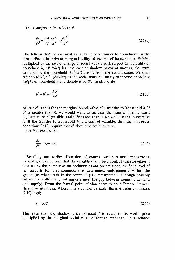
(a) Transfers to households, rh.

aL aw ad aXh -_=-_--_v_,

arh ad arh arh (2.13a)

This tells us that the marginal social value of a transfer to household h is the direct effect (the private marginal utility of income of household h, dvh/arh, multiplied by the rate of change of social welfare with respect to the utility of household h, aW”/av”) less the cost at shadow prices of meeting the extra demands by the household (axh/arh) arising from the extra income. We shall refer to (aWh/avh).(avh/arh) as the social marginal utility of income or welfare weight of household h and denote it by /Ih; we also write

so that bh stands for the marginal social value of a transfer to household h. If bh is greater than 0, we would want to increase the transfer if an upward adjustment were possible, and if bh is less than 0, we would want to decrease it. If the transfer to household h is a control variable, then the first-order conditions (2.10) require that bh should be equal to zero.

(b) Net imports, ni.

aL !n,=vi-lIPT. (2.14)

Recalling our earlier discussion of control variables and ‘endogenous’ variables, it can be seen that the variable ai will be a control variable either if it is set by the planner as an optimum quota on net trade, or if the level of net imports for that commodity is determined endogenously within the system (as when trade in the commodity is unrestricted - although possibly subject to tariffs - and net imports meet the gap between domestic demand and supply). From the formal point of view there is no difference between these two situations. Where ni is a control variable, the first-order conditions (2.10) imply

vi = pup:. (2.15)

This says that the shadow price of good i is equal to its world price multiplied by the marginal social value of foreign exchange. Thus, relative

18 J. Drdze and N. Stern, Policy rejivm and market prices

shadow prices within the set of goods for which ni is a control variable are equal to relative world prices.

We have, therefore, derived a standard rule for relative shadow prices of traded goods in cost-benefit analysis - they are equal to relative world prices. The model we have constructed allows us to see clearly the conditions under which this result holds. The crucial feature is that public production of any of the commodities under consideration can be seen as displacing an equivalent amount of net imports, and moreover the general equilibrium repercussions involved are mediated exclusively by the balance of payments constraint. Formally, this can be seen from the fact that, in eq. (2.13) the vector y1 enters the Lagrangian in exactly the same capacity as the vector z, except for its presence in the balance of payments constraint.

That this is the crucial condition should be intuitively clear from the economics of the problem. An extra demand for an imported good will generate a foreign exchange cost and thus create a cost given by its world price multiplied by the marginal social value of foreign exchange. If there is no other direct effect in the system, then all the relevant general equilibrium repercussions are captured in the marginal social value of foreign exchange and we have found the shadow price of the good. If, however, there is a direct effect of increasing net imports somewhere else in the system, then the world price (multiplied by p) will no longer be equal to the shadow price.

One example of the latter complication would arise with an exported good for which world demand was less than perfectly elastic. One might think it sufficient in this case simply to replace the world price by the marginal revenue in the shadow price formula (2.15). This is correct if the domestic price of the good can be separately controlled. If it cannot (because, say, the indirect tax on the good is predetermined and cannot be influenced by the planner) then the calculation of the shadow price should take into account the effects on private sector supplies and profits of the fall in the world price as a result of extra public production.

A second example would arise if there were separate foreign exchange budgets for different sectors which were set outside the control of the planner. If a sector is identified by its group of commodities, then within a sector relative shadow prices of traded goods would be equal to relative world prices, but across sectors this would not apply since the marginal social value of foreign exchange across sectors would no longer be equal. This is a further example of the importance for shadow prices of being clear as to just what the planner controls. If the planner also controlled the allocation of foreign exchange across sectors then the correct rule would be to allocate across sectors so that the marginal social value of foreign exchange across sectors would be equal, and then relative shadow prices for traded goods would be equal to relative world prices for all goods.

J. DrLze and N. Stern, Policy reform and market prices 19

(c) Producer rations, ji.

-=vY+& dL

& a_Vi ayi’

where

b-xehbh h

(2.16)

(2.17)

and bh is as in eq. (2.13b). The expression (2.16) is most easily interpreted if we think of good i as the output of the firm and of ji as the amount it is required to produce. Then an increase in the required output will require extra inputs and the overall change in the production vector will be ay/& with value at shadow prices given by the first term on the right-hand side of (2.16). The increase in required output will also affect the profits of the firm and this is captured in the second term on the right-hand side of (2.16) - b is the weighted sum of the marginal social values of transfers to households with weights given by the shares of the households in the profits of the firm. Using the properties of the functions y and xc, and noting in particular that ayi/aji= 1, we can rewrite (2.16) as

L=Vi-MSCi+b(pt-MC,), %i

where

MCi~-Cpjayj j#i Qi

(2.18)

(2.18a)

is the marginal (private) cost of good i (i.e. the value at market prices of the inputs required to produce an extra unit), and

MSC,= - 1 vj% j#i $5

(2.18b)

is its ‘marginal social cost’ (i.e. the value at shadow prices of the same inputs).

If ji is a control variable, then the expression in (2.18) must be zero and we have

Vi= MSCi- b(pi- MC,). (2.19)

This states that the shadow price of good i is its marginal social cost, corrected by the marginal social value of the relevant profit effects.


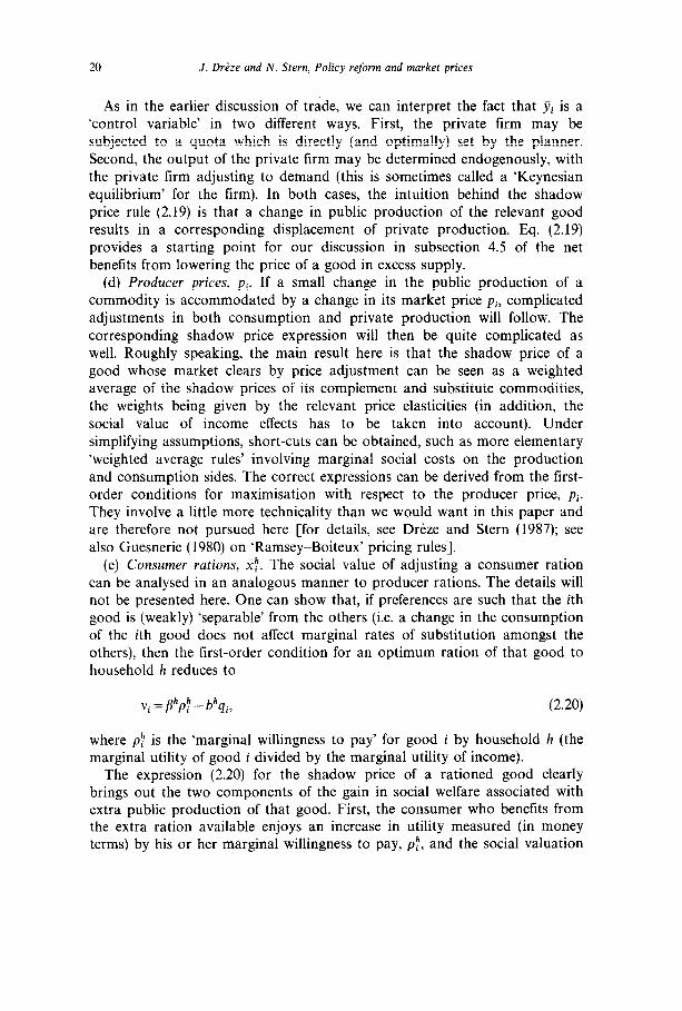
As in the earlier discussion of trade, we can interpret the fact that yi is a ‘control variable’ in two different ways. First, the private firm may be subjected to a quota which is directly (and optimally) set by the planner. Second, the output of the private firm may be determined endogenously, with the private firm adjusting to demand (this is sometimes called a ‘Keynesian equilibrium’ for the firm). In both cases, the intuition behind the shadow price rule (2.19) is that a change in public production of the relevant good results in a corresponding displacement of private production. Eq. (2.19) provides a starting point for our discussion in subsection 4.5 of the net benefits from lowering the price of a good in excess supply.

(d) Producer prices, pi. If a small change in the public production of a commodity is accommodated by a change in its market price pi, complicated adjustments in both consumption and private production will follow. The corresponding shadow price expression will then be quite complicated as well. Roughly speaking, the main result here is that the shadow price of a good whose market clears by price adjustment can be seen as a weighted average of the shadow prices of its complement and substitute commodities, the weights being given by the relevant price elasticities (in addition, the social value of income effects has to be taken into account). Under simplifying assumptions, short-cuts can be obtained, such as more elementary ‘weighted average rules’ involving marginal social costs on the production and consumption sides. The correct expressions can be derived from the lirst- order conditions for maximisation with respect to the producer price, pi. They involve a little more technicality than we would want in this paper and are therefore not pursued here [for details, see Dreze and Stern (1987); see also Guesnerie (1980) on ‘Ramsey-Boiteux’ pricing rules].

(e) Consumer rations, 2:. The social value of adjusting a consumer ration can be analysed in an analogous manner to producer rations. The details will not be presented here. One can show that, if preferences are such that the ith good is (weakly) ‘separable’ from the others (i.e. a change in the consumption of the ith good does not affect marginal rates of substitution amongst the others), then the first-order condition for an optimum ration of that good to

household h reduces to

vi = p”p; - bhqi,

where pf is the ‘marginal willingness to pay’ for good i by household h (the marginal utility of good i divided by the marginal utility of income).

The expression (2.20) for the shadow price of a rationed good clearly brings out the two components of the gain in social welfare associated with extra public production of that good. First, the consumer who benefits from the extra ration available enjoys an increase in utility measured (in money terms) by his or her marginal willingness to pay, p:, and the social valuation

J. DrPze and N. Stern, Policy reform and market prices 21

of this change in private utility is obtained by using the usual ‘welfare weights’, ph. Second, a transfer of income occurs, as the same individual is required to pay the consumer price, qi, for the extra ration; the social

evaluation of this second effect relies on the marginal social value of a transfer to the concerned consumer, bh.

This formulation can be adapted to give us shadow prices for important special cases, e.g. public goods and the hiring of labour in a rationed labour market (see section 3). Public goods, for instance, can be modelled here as a rationed commodity - everyone has to consume the same amount, i.e. that which is made available - with a zero price. Analogously to expression (2.20), and under the same assumption of ‘separability’, we then obtain the shadow price of a public good as xh /3” p:, the aggregate, welfare-weighted, marginal willingness-to-pay.

If the separability assumption is violated, expression (2.20) will involve an extra term that captures the marginal social value of the resulting substitution effects. Alternatively, this extra term can be seen as reflecting the effect on the ‘shadow revenue’ of the government - a notion explored in detail in section 3.

(f) Indirect taxes, ti

(2.21)

This can be reformulated after decomposing ax/aq, into an income and a substitution effect (and using the symmetry of the Slutsky terms) to give

g= -;b”xf+(q-v)$, 1

(2.22)

where L)(q,Zh, u”) is the compensated demand of consumer h for good i, and z$z~,$‘. Thus, the jth component of the vector a&/aq is the compensated response in aggregate consumption of good i to the price of good j. If ti is a control variable, then we have

tC 3 = c bhx;, aq h

(2.23)

where rc = q - v is a vector of ‘shadow consumer taxes’ equal to the difference between consumer prices and shadow prices. If, under a suitable normalisa- tion rule, shadow prices, v, are equal to producer prices, p, then rc reduces to the indirect tax vector, t, and expression (2.23) precisely amounts to the

22 J. Dr.&e and N. Stern, Policy reform and market prices

familiar ‘many-person Ramsey rule’ [see, for example, Diamond (1975) and Stern (1984)J

We see, therefore, that expression (2.23) gives us a remarkably simple generalisation of the standard optimum tax rules. The kind of economies where the standard rules are derived happen, in fact, to be economies for which shadow prices are proportional to producer prices [as in Diamond and Mirrlees (1971)]. What we have now seen is that the same rules apply in much more general economies if we simply replace producer prices by shadow prices.

Much of the discussion of the structure of indirect taxes and the balance between direct and indirect taxation also carries through on replacing actual taxes by shadow taxes. One can show, for example, that if there is an optimum poll tax, households have identical preferences with linear Engel curves, and labour is separable from goods, then shadow taxes should apply at a uniform proportionate rate [see Dreze and Stern (1987) and Stern (1987)]. Note that if shadow prices are not proportional to producer prices, this means that actual indirect taxes should not be uniform.

3. Shadow prices and the macro economy

We shall now investigate the relation between the theory developed so far and more familiar considerations of public tinance and macroeconomic policy. These two themes are treated in subsections 3.1 and 3.2, respectively.

3.1. Public finance and the shadow revenue

If the public sector trades at prices p we can calculate its net revenue, R,, as the sum of profits in the public sector, pz, the value of the foreign exchange sold, cpF (where cp is the exchange rate), revenue from indirect taxes, tx, tariff revenue, (p - qpw)n, the government’s share of private profits, crc, which includes profits taxes, and lump-sum taxes, -&rh:

R,~pz+cpF+tx+(p-cpp”)n+in-Crh. h

(3.1)

It is important to recognise that this expression for R, gives us the net revenue for the government in a way that is different from the standard procedures in published government accounts in a number of important respects. First, it takes the revenue and expenditure accounts together. If we were to separate the elements of R, in (3.1) we might think of ( -pz +ci, rh) as government expenditure and of the remaining terms as revenue, with the net revenue being the difference between the two. However, there is nothing compelling in this particular way of making the distinction since, in fact,

1. D&e and N. Stern, Policy reform and market prices 23

many different components of R, could turn out to be either positive or

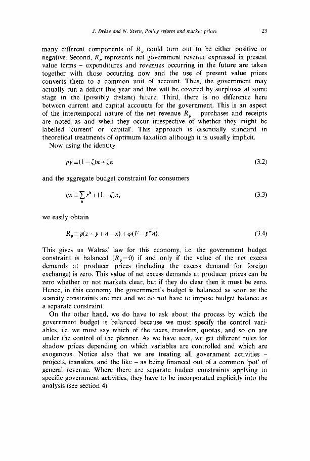
negative. Second, R, represents net government revenue expressed in present value terms - expenditures and revenues occurring in the future are taken together with those occurring now and the use of present value prices converts them to a common unit of account. Thus, the government may actually run a deficit this year and this will be covered by surpluses at some stage in the (possibly distant) future. Third, there is no difference here between current and capital accounts for the government. This is an aspect of the intertemporal nature of the net revenue R, - purchases and receipts are noted as and when they occur irrespective of whether they might be labelled ‘current’ or ‘capital’. This approach is essentially standard in theoretical treatments of optimum taxation although it is usually implicit.

Now using the identity

py-(l-&+jn

and the aggregate budget constraint for consumers

qx=Crh+(l --&I, h

(3.2)

(3.3)

we easily obtain

R,-p(z+y+n-x)+cp(F-p”n). (3.4)

This gives us Walras’ law for this economy, i.e. the government budget constraint is balanced (R,=(l) if and only if the value of the net excess demands at producer prices (including the excess demand for foreign exchange) is zero. This value of net excess demands at producer prices can be zero whether or not markets clear, but if they do clear then it must be zero. Hence, in this economy the government’s budget is balanced as soon as the scarcity constraints are met and we do not have to impose budget balance as a separate constraint.

On the other hand, we do have to ask about the process by which the government budget is balanced because we must specify the control variables, i.e. we must say which of the taxes, transfers, quotas, and so on are under the control of the planner. As we have seen, we get different rules for shadow prices depending on which variables are controlled and which are exogenous. Notice also that we are treating all government activities - projects, transfers, and the like - as being financed out of a common ‘pot’ of general revenue. Where there are separate budget constraints applying to specific government activities, they have to be incorporated explicitly into the analysis (see section 4).

24 .I. D&e and N. Stern, Policy reform and market prices

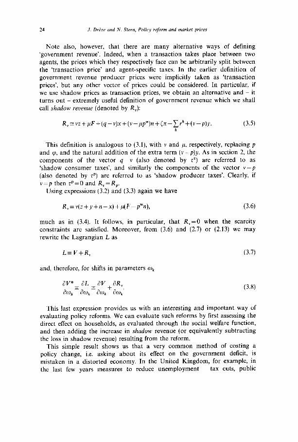
Note also, however, that there are many alternative ways of defining ‘government revenue’. Indeed, when a transaction takes place between two agents, the prices which they respectively face can be arbitrarily split between the ‘transaction price’ and agent-specific taxes. In the earlier definition of government revenue producer prices were implicitly taken as ‘transaction prices’, but any other vector of prices could be considered. In particular, if we use shadow prices as transaction prices, we obtain an alternative and - it turns out - extremely useful definition of government revenue which we shall call shadow revenue (denoted by R,):

R,,-vz+@‘+(q-v)x+(v-pp”)n+i~xrh+(v--p)y. h

(3.5)

This definition is analogous to (3.1), with v and p, respectively, replacing p and cp, and the natural addition of the extra term (v-p)y. As in section 2, the components of the vector q-v (also denoted by rc) are referred to as ‘shadow consumer taxes’, and similarly the components of the vector v-p (also denoted by rp) are referred to as ‘shadow producer taxes’. Clearly, if v=p then rp=O and R,=R,.

Using expressions (3.2) and (3.3) again we have

R,=v(z+y+n-x)+,u(F-f’n), (3.6)

much as in (3.4). It follows, in particular, that R,=O when the scarcity constraints are satisfied. Moreover, from (3.6) and (2.7) or (2.13) we may rewrite the Lagrangian L as

L=V+R, (3.7)

and, therefore, for shifts in parameters wk

(3.8)

This last expression provides us with an interesting and important way of evaluating policy reforms. We can evaluate such reforms by first assessing the direct effect on households, as evaluated through the social welfare function, and then adding the increase in shadow revenue (or equivalently subtracting the loss in shadow revenue) resulting from the reform.

This simple result shows us that a very common method of costing a policy change, i.e. asking about its effect on the government deficit, is mistaken in a distorted economy. In the United Kingdom, for example, in the last few years measures to reduce unemployment - tax cuts, public

.I. Drtbe and N. Stern, Policy reform and market prices 25

expenditure programmes, employment subsidies, and the like - have been extensively discussed and it has been common practice to evaluate their cost in terms of the implied savings or losses of public revenue. This is, indeed, the spirit of many simplistic applications of the fashionable ‘cost-effectiveness’ criterion. Eq. (3.8) shows us that this approach is incorrect. If we are to cost our policies correctly we should be using shadow revenue and not actual revenue. We should emphasise again that this does not neglect issues of financing since Walras’ law tells us that satisfying the scarcity constraints will imply budget balance by whatever methods have been incorporated into the specification of the model.

This example, and (3.8), indicate that there is no need in this framework for a separate concept of the shadow price of government revenue. Govern- ment revenue (unlike foreign exchange) is not a separate good here. The shadow prices take account systematically of all the repercussions of a project including those which operate via the readjustment of public finances.

3.2. Some macroeconomic considerations

We now turn to some important macroeconomic aspects of shadow price systems: savings, foreign exchange, shadow wages, and shadow discount rates. In discussing the concepts of savings and discount rates we must give the model an intertemporal interpretation by indexing commodities by the date at which they appear. Prices and budget constraints are to be interpreted in present value terms.

It is often argued that developing countries should place a special premium on savings, i.e. that for some reason savings are too low and that it is important to provide measures to increase them. This position is not always clearly argued. The statement that savings are too low implies a judgement on the intertemporal allocation of consumption (since to increase savings is to increase the welfare of the future generations relative to current ones) which may not be easy to make. Moreover, savings rates in developing countries are now commonly around 20 percent, which does not suggest immediately that savings are ‘too low’.

It is possible, within our framework, to give precision to the notion of a premium on savings. We can write the expression for bh (2.13b) as

bh = 8” -c 3 MPCfz,

i. r 4ir (3.9)

where, MPCFT is the marginal propensity of household h to spend on the ith good in period z

J. D&e and N. Stern, Policy reform and market prices

(3.10)

We can then see that the marginal social value, bh, of a transfer to household h is higher, the higher is its propensity to spend on goods in periods when the shadow price is low relative to the market price (low vi,/qi,). If current period commodities are relatively more valuable than future period commodities, then, other things being equal, there will be a higher value attached to transfers to those with a higher propensity to save. In this context we should think of a household as representing a dynasty which takes full account of the future welfare of descendants in its own utility function. If the government thinks it has a responsibility to give weight to future generations over and above that which arises from households’ concern for their own descendants, then this might induce a separate argument for a premium on savings.

The model we have described so far contains a shadow price on foreign exchange, p, and it is tempting to compare it with the exchange rate, cp, i.e. the price of a unit of foreign exchange. The simple comparison, however, contains no information since we can choose any absolute level of p by resealing the shadow price vector (v,~) without changing anything real. The marginal social value of foreign exchange will also depend on the way in which the balance of payments is secured; an example will both illustrate this and provide a possible definition of a premium on foreign exchange which would be of substance.

Suppose that an import quota applies to the first good and that this quota can be set by the planner, or (equivalently for our purposes) that it adjusts endogenously to ensure the balance of payments. Then n, is a control variable and from (2.14) we have

VI -ppy=o. (3.11)

Suppose further that the producer price for the good is simply the import price (cpp; in domestic prices) plus a tariff t{ so that

Pl =cppY+C. (3.12)

Then

P wG+t: Vl -= cp ( 1 cpp; P,’

(3.13)

using expressions (3.11) and (3.12). Therefore, if the tariff is positive we have


c is greater than 2, cp Pl

(3.14)

or the shadow price of foreign exchange as a proportion of the market price is greater than the corresponding ratio for good 1. We may then say that there is a premium on foreign exchange in the sense of expression (3.14) and that this premium can be measured by the term in parentheses in (3.13) i.e. the extent to which the producer price of good 1 is above the world price. The analysis may be generalised in a straightforward way if the balance of

payments is achieved not solely through the first good but by adjusting the quotas for a fixed bundle of goods - the premium is then given by the ratio between the value at producer prices and the value at world prices of that bundle. This idea is commonly embodied in manuals on cost-benefit analysis [see, for example, Dasgupta, Marglin and Sen (1972) who use a shadow exchange rate along these lines, or Little and Mirrlees (1974) who work in terms of a standard conversion factor for converting the value of broad groups of commodities from market prices to shadow prices].

The appropriate cost of labour is a further topic that has received great attention in discussions of policies and shadow prices in developing countries. It is often argued, for example, that if market wages are kept above the marginal product of labour elsewhere in the economy, then there will be a bias against employment and techniques of production will be more capital intensive than they ‘should’ be. The model that we are using embodies fixed prices and rationing and can, therefore, be used to derive an expression for shadow wages in the context just described.

The shadow wage will depend on just how the market for labour (indexed hereafter by 8) functions. For a simple but important example we shall think of a model where total labour is fixed and residual labour not employed in the formal sector is absorbed in self-employment. We can think of a peasant farm or family firm owned by a single household. We shall index this firm by g and it is to be distinguished from the single private firm of the model as previously defined which we shall think of as being a formal sector firm employing labour at a wage pe. We consider the suppliers of labour to be rationed in the amount of work they can sell to the formal sector (i.e. they would like to work more). Under these assumptions, we can regard employment in firm g, the peasant farm (owned by a single household h), as being determined by an endogenous quota j s. The corresponding first-order condition Cjust as in expression (2.16)] is then

(3.15)


where x9 is the profit in the gth firm (which goes entirely to the hth household). We can rewrite the right-hand side of expression (3.15) [as in (2.19)] to give

v, = MSPS, - b*(p, - MI'?), (3.16)

where MP$ is the marginal product of labour in firm g( -~j+epj(~yJ9/&$!))

and MSP; is its marginal social product of ( -~jze~j(~y3/@$)). This is precisely the shadow wage of Little-Mirrlees (1974, pp. 27&271).

The interpretation of expression (3.16) should be intuitively clear. The social cost of employing labour is the social value of what it would otherwise have produced less the marginal social value of the gains in income for household h. One can also consider different types of alternative activity where, for example, those who are not employed in the formal sector do not work but receive unemployment benefit. Then MSP$ is replaced by the value of leisure, or reservation wage, adjusted by the welfare weight, and the income change is now the difference between the market wage and the unemployment benefit. The model can be adapted to deal with several interesting examples of unemployment. Migration equilibria can also be captured through extra constraints of the form, say, oR(.)=g”(.), where R and U are indices for rural and urban households, respectively.

The last example of a broad macroeconomic issue that we shall discuss here is the shadow discount rate. In order to define this we must make the intertemporal features of the problem more explicit. Assuming the project does not come along with a gift of foreign exchange (dF=O) we can think of its social value, S, as vdz. Indexing now explicitly on time we have

SsvdzECv,dz,=C Cvirdzi,, T i 7

(3.17)

where dzi, is the change in public supplies of good i in period z, dz, is the vector (dz,), and similarly for Vi* and v,. When we discuss discounting we focus on the shadow price (or marginal social value) of the numeraire commodity in year r relative to its shadow price in other years. This, of course, requires the specification of a numeraire relative to which social profitability is measured in each year. Formally we may write

vir-v. a IT C’ (3.18)

where Vi, is the vector of shadow prices for year z normalized relative to the numeraire and a, is the shadow discount factor. The shadow discount rate, pr, is then defined as


a,-a,+1 PFa .

7+1

(3.19)

The process of going through expressions (3.17)-(3.19) is essentially unavoid- able in defining the social discount rate since the notion precisely concerns the rate at which the marginal social value of the numeraire is falling over time. If we take commodity i as the numeraire, then the shadow discount rate simply becomes

PI= vir-Vi,r+l

Vi,r+ 1

It is clear from eq. (3.20) that the choice of numeraire will affect the shadow discount rate unless the relative shadow prices of alternative numeraire commodities are constant over time, i.e. if pr is the shadow discount rate using i as numeraire and pi is the shadow discount rate when j is used as numeraire, then

Pr - Pi, ifand only if !k=w (3.21) Vjr vj,z+l

We cannot, therefore, answer the question, ‘What should be the shadow discount rate? without being told, or without our choosing, what the numeraire is to be. And the apparent difference between the shadow discount rates proposed in alternative methods of cost-benefit analysis should not mislead us into thinking that the differences are necessarily real - alternative methods may simply involve different units of account.

One particularly easy and transparent choice for the numeraire in each year is foreign exchange. Trading in foreign exchange from one year to the next (i.e. borrowing and lending on world capital markets) can be seen as a form of production activity which we can think of as being undertaken by a public sector firm. If this firm is maximising its profits at shadow prices, as it should (see section 4), then its marginal rate of transformation of foreign exchange in the future into foreign exchange now will be given by the relevant interest rates ruling in the world capital markets. The rate of fall of the social value of a unit of foreign exchange is then equal to the interest rate on world capital markets. Therefore, the shadow discount rate will be equal to the rate of interest on world capital markets when foreign exchange in each year is the numeraire. Notice that the numeraire in this example is foreign exchange in the hands of the government. As we saw in our discussion of the marginal social value of transfers and the net social marginal utility of income [see (2.13b) and (3.8b)] the valuation of income

J.P.E. B

30 J. Drtize and N. Stern, Policy reform and market prices

in the hands of other agents will differ from that in the hands of the government.

The values of the broad variables we have been examining here may be seen as major determinants of the appropriate level of investment, its allocation across industries, and its intensity in different factors of production. But it would not be correct to see these variables as exogenous so that the chain of causation flows from them to the appropriate level of investment. One should think of the shadow prices and the investment level as being determined simultaneously within the same model. And neither would it be correct to think of just one of these variables, say the shadow discount rate, as determining or being determined by the size of the investment budget. Whether or not a project should be accepted depends on the whole vector of shadow prices and not on one single aspect of them, so that the overall level of investment as determined by this method of project selection depends on all the shadow prices.

4. Shadow prices, market prices, and the private sector

Our concern in the previous section was with public revenue and macroeconomic considerations; we now examine the implications of our theory for policy towards the private sector. We shall be particularly concerned with the relationship between public and private production, and with defining the circumstances and sense in which certain market prices may be reliable guides to policy-making even in distorted economies. We begin the discussion by examining (in subsection 4.1) the relation between projects and plans; we then look (in subsection 4.2) at efficiency in the public sector and between public and private sectors; project appraisal for private firms, and for public firms with separate budget constraints, are examined in subsection 4.3. In subsection 4.4 we discuss the relation between shadow prices and market prices. Finally, in subsection 4.5 we ask about price reform and, in particular, examine the question of whether the price of a good in excess demand should be increased.

4.1. Projects and plans

So far, our examination of public production decisions has been confined to small projects defined as changes dz undertaken from an arbitrary initial public production plan. In particular, while we have assumed that (subject to the scarcity constraints) the levels of control variables available to the planner were chosen optimally, we have not assumed that the public production plan itself had been optimised. Thus, our theory of shadow prices and policy appraisal does not assume either the optimisation of public production or even the knowledge of public production possibilities.


It is clear, therefore, that since the theory we have presented applies to an arbitrary public production plan, it applies in particular to the situation where the initial public production also happens to be a socially optimum one. Of course, the values taken by shadow prices are generally different if evaluated at a different public production plan; but the rules determining them will not change as long as the controls available to the planner are the same. This point is worth emphasising, because it has caused confusion in the literature [see Dr&ze and Stern (1987) and Dinwiddy and Teal (1987) for further elaboration].

Moreover, while shadow prices have been defined for an arbitrary public production plan, it is important to realise that they provide crucial signals for the improvement and optimisation of public production decisions. This is so not only because, as we have seen, shadow prices allow a straightforward identification of socially desirable projects; in addition, it can be shown that under fairly general conditions a socially optimum public production plan is one that maximises profits at shadow prices. To see this, let 2 represent the set of feasible public production plans. Let also z* be a socially optimum production plan [formally, a production plan which maximises V*(z;o) within Z], and v* the corresponding vector of shadow prices. If, at z*, some feasible project dz existed with v*dz greater than 0, then z* would not be optimum, since v*dz greater than 0 indicates that dz increases welfare; hence, it must be true that at z* no feasible project dz shows a profit at shadow prices. If Z is convex, this in turn implies that z* maximises shadow profits (in Z) at the shadow prices v*, since otherwise a small move in the direction

of some production plan with greater shadow profits would represent a feasible project. Thus, when public production possibilities are convex, a socially optimum public production plan is one that maximises shadow profits.

4.2. Public efficiency and private efficiency

Given some initial public production plan, we have a set of shadow prices, v. These shadow prices should be used by all public sector firms except (i) public sector firms facing an independent revenue constraint (this is discussed in the next subsection), and (ii) public sector firms that generate externalities. All public sector firms to which these two qualifications do not apply should, moreover, choose a production plan that maximises shadow profits (if they know their production set and the latter is convex). For those firms taken together, therefore, production should be efficient. This may seem an unremarkable result, but it can have quite strong implications - see, for example, subsection 4.4.

There is no general reason to suppose that public sector and private sector firms taken together should be efficient, although under certain circumstances


this may be desirable. For example, we can show that when we make some quite strong assumptions, shadow prices v will be proportional to producer prices p and government and private firms taken together should be efficient (see subsection 4.4).

4.3. Private firms and budget-constrained public firms

The projects dz we have considered so far have been explicitly in the public sector. The government may also wish to appraise private sector projects - for example, for the purpose of granting licenses. The essential difference in the model between a public and a private project representing the same change in net supplies lies in who receives the profits; this difference is reflected in the nature of the prices appropriate for appraising public and private projects.

Formally, we can introduce into the model a private firm (indexed by 0) whose production plan, y”, is regarded as a vector of predetermined variables. A private project, dy’, then induces a change in welfare, dK where

d I,’ = o dye = v dye + b”(p dye), 8L’

(4.1)

where b” is the average of the marginal social values of transfers (bh) for the shareholders of the firm, weighted by their shares in the firm’s profits (b” =ch oohbh, where eoh is the share of the hth household). Thus,

dI’=(v+b’p)dyO. (4.2)

The appropriate price vector for the evaluation of private projects is therefore a straightforward weighted sum of shadow prices for public projects and of market prices, with weights reflecting the marginal social value of private profits. It should be noted that it is possible, or even likely for some firms, that b” will be negative; indeed, shareholders are rarely regarded as priority targets for income transfers from the government.

A similar result arises if the firm belongs to the public sector but is subject to a budget constraint of the form

py" = co, (4.3)

for some price vector p. The analysis proceeds much as in the previous problem. The Lagrangian now includes a term b”(pyO-E’), where b” is the Lagrange multiplier on constraint (4.3), and for a project dye we have

dV=(v+b”p)dyo. (4.4)


The appropriate price vector for evaluating projects in this public lirm is

then a weighted sum of the shadow price vector and the vector of prices defining the firm’s budget constraint - the latter may, of course, be the vector p of market prices. Note, however, that for a feasible project dye preserving (4.3), i.e. a project satisfying p dye = 0, expression (4.4) reduces to d I/ = v dy’. In other words, an alternative and simpler way of formulating socially desirable production decision rules for budget-constrained public firms is to state that such firms should seek to improve profits at ordinary shadow prices within the possibilities compatible with their budget constraint. Budget constrained public firms are quite common in practice where public firms have performance criteria related to profit, or are separately organised, and this case is therefore of some importance.

We can use the analysis of this section to examine the issue of ‘privatisation’. Suppose it is suggested that some production be transferred to the private sector in the sense that the public sector production plan is modified by dz and a private sector firm is relied upon to make a compensating adjustment. If the private sector does things differently from the public sector, then the private firm’s production change, dy’, may not be exactly the converse of dz. The social value of the change is then, using expression (4.2),

dV=(v+b’p)dy’-vdz, (4.5)

which may be written

d I/ = v(dyO - dz) + hop dy’. (4.6)

The social value of the change then consists of an efficiency effect associated with the difference in the production changes, dye and dz, evaluated at shadow prices and a distributional effect associated with the transfer of profits. If the marginal social value of the income of profit receivers is negative, then the second term in expression (4.6) will be negative. This will have to be adjusted if there is a payment from the purchasers of the privatised activity since this represents a transfer to the government. If the payment is less than the (discounted) value of the profits stream, then there is a net outflow of public funds which would probably count negatively.

One then has to ask whether this loss of funds is outweighed by any efficiency gain. Leaving aside the empirical evidence on private versus public efficiency (which appears ambiguous), it must be emphasised that the difference in production vectors should be evaluated at shadow prices. There are, moreover, no incentives for private firms to economise on inputs at shadow prices, whereas government firms can, in principle, be directed to do so. The issues included in this analysis do not therefore provide a strong presumption that privatisation will yield net social benefits. There are

34 J. Drize and N. Stern, Policy reform and market prices

obviously wider and important issues that this analysis omits, including difficulties of information, organisation and incentives in public relative to private firms, but they should be set carefully against those we have succeeded in capturing here.

4.4. Market prices and shadow prices

We derived in section 2 a number of rules which should be satisfied by shadow prices, and saw that these rules varied according to which variables could be controlled by the planner. We now focus on the relationship between shadow prices and market prices. Throughout this section it must be borne in mind that we are concerned with relative prices - thus, when we speak (say) of shadow prices and market prices being ‘equal’, we really mean ‘proportional’.

It is fair to say that the conditions that ensure that (relative) shadow prices are equal to (relative) producer prices are, generally, rather restrictive. Perhaps the most important example of a set of conditions that ensures this equality is given by the well-known model of Diamond and Mirrlees (1971), where (i) all goods can be taxed and indirect taxation is fully under the control of the planner; (ii) private production is competitive and production sets are convex; (iii) private profits, if any, are fully taxed; and (iv) no quantity rationing applies to private producers (the only exception being that a quantity signal may determine the production plan of industries with constant returns within their supply correspondence). Roughly speaking when these assumptions are satisfied the private sector is effectively under full government control: by setting the appropriate set of producer prices the government can induce the private firm to produce at any relevant point that it wishes, and this has no direct repercussions on the consumer sector since profits are fully taxed and consumer prices can be manipulated separately. The optimum will therefore be the same as if the private firm were part of the public sector, and the marginal rates of transformation in the private firm will therefore be equal to shadow prices. They are also equal to market prices (since private production is competitive) and therefore shadow prices are equal to market prices.

An alternative set of conditions ensuring the equality of shadow prices and producer prices, which does not involve the restrictive assumption of optimum indirect taxation, consists of the conditions underlying the so-called ‘non-substitution theorem’: constant returns to scale, a single scarce factor, no joint production, and competition (without rationing) among private producers. See Diamond and Mirrlees (1976) and Dreze and Stern (1987) for further discussion of this result and those of the preceding paragraph.

Apart from restrictive models of the kind involved in these two examples, one would not usually expect to find shadow prices equal to producer prices.


But we can still ask whether shadow prices, or a subset of them, will coincide with other kinds of market prices. The principal case of this coincidence is where shadow prices for traded goods are equal to world prices. We saw in section 2 that the conditions for this to be true are fairly general, and basically involve the relevant goods being traded without quota, or the quotas being optimally selected.

Where shadow prices are not equal to world prices, we can in many cases see them as a weighted average of marginal social costs of goods drawn from production and from consumption (see subsection 2.4), with weights reflecting quantities drawn from each side. This will not be the same, however, as a weighted average of consumer and producer prices. One can derive rules along these lines [see Drlze and Stern (1987)], but the weighting procedure is much more complicated and involves averaging (using matrices of demand derivatives) across all markets taken together.

A case where market prices and shadow prices have a strong link, although they do not coincide, is related to the existence of constant-returns- to-scale firms. If there are no quantity constraints on such firms (other than the ‘scale factor’, determining a firm’s production plan within its supply correspondence) and they make zero profits, then one can show that they should also make zero profits at shadow prices. Intuitively, one can understand the result as.$ollows. A small public project using the same input and output proportions as a private firm operating under constant returns could be accommodated in the general equilibrium if the production plan of the private firm were correspondingly displaced. This public project would then have no effect on social welfare since no household welfare level has changed. It should therefore ‘break even’ at shadow prices. But this project was simply a scaled down version of the activity of the private firm and therefore that firm would also break even at shadow prices. From a formal point of view this result can be derived by examining the first-order conditions for the scale factor of the firm, which may be regarded as a control variable.

The result does not allow us to say that producer prices are equal to shadow prices since the condition on one firm provides only one linear constraint on the I vector of shadow prices. If it holds for several constant- returns-to-scale firms, then it can narrow down considerably the difference between shadow and producer prices. It must be remembered, however, that the condition is only relevant if the constant-returns firms should be operating at a strictly positive scale at the optimum level of the controls. We would not expect to find producer prices equal to shadow prices unless the conditions of one of the two examples above are met.

When there is a binding quota on the output of a firm, the question naturally arises whether the corresponding good should be devalued in the shadow price system relative to the producer price system. From expression


(2.19) one can show (abstracting from distributional considerations) that the accounting ratio, vi/pi, of a good i in excess supply is lower than a weighted average of the accounting ratios of its inputs by a fraction measuring the discrepancy between price and marginal cost [see (4.7)]. Hence, the intuitive presumption that a good in excess supply is overvalued in the producer price system does have some content. A discussion of how prices should be reformed in this context is provided in the next subsection.

We have seen, therefore, that while it is not usually true that shadow prices coincide with market prices in a distorted economy, quite a lot can be said about how they might diverge.

4.5. Price reform

Should we lower the price of a good in excess supply and increase the price of a good in excess demand? The average economist’s tirst reaction would be ‘yes’, but it would or should also be acknowledged that a whole range of factors may invalidate this recommendation. The basic principles of policy analysis in distorted economies can point us to what might go wrong and direct any empirical enquiry that is necessary to check whether the economist’s initial response is reliable. We provide in this subsection an analysis which both gives an example of how the approach can guide applied analysis and judgement, and yields some results on the important problem of the reform of controlled economies. As with privatisation we focus on those aspects of rationing and price reform which can be illuminated by the theory. There is no discussion here, for example, of attempts to influence rations - we do not discuss rent-seeking.

We begin with the case of excess supply and rationed producers and then look at excess demand and rationed consumers. We consider the producer price of good i, pi, to be an exogenous parameter, which is currently fixed at a level which is ‘too high’ in the sense that the consumers (who are not rationed for this good) demand less at the price they face, qi, than the lirm would like to supply at the price pi. This is captured by the existence of a binding constraint, jji, applying to the firm’s production of good i. The variable ji acts as the equilibrating variable on the ith market.

Since yi is an endogenous variable we have eq. (2.19). To reiterate the latter

Vi = MSCi - b(pi - MC,),

where MSCi is the value at shadow prices of the marginal inputs required to produce an extra unit of the ith good [see (2.18b)l. If b is small enough, i.e. profit taxes are not too far from optimum, then given pi> MCi, we may write

J. Dr&e and N. Stern, Policy reform and market prices 37

(4.7)

where aj is the share of the jth input in the marginal cost (the aj sum to one for j#i). Eq. (4.7) says that, under the given assumption, the accounting ratio, vi/pi, for the ith good is less than a weighted average of the accounting ratios of the inputs, the weights being given by the respective shares in marginal cost. In this sense the good in excess supply is devalued in the shadow price system relative to the market price system.

We want now to look at the marginal social value of lowering the market (producer) price, p;, of a good which is in excess supply. The ‘standard ._ . reaction’ is justified if al’*/& ~0. From (2.11) we have

av* aL -=- 8th aPi’

which gives us, using (2.13) and (2.17),

av* ap- = -~phx+i

L h

If we decompose axj/dqi into income and substitution effects we have

av* api -vc 1 ay aa _d,

api aqi ”

(2.11’)

(4.8)

(4.9)

where 8P/aqi is the vector of aggregate substitution effects, sij, and di is a ‘net distributional characteristic’, defined by di z xh bhxf - byi. The latter captures the pure income effects associated with an increase in the ith price. If, as we are assuming, the ith output is rationed, then dy/dpi is zero and aV*/dp, is given by

av* _=- aPi

(4.9a)

The sign of di depends on how far the consumers and shareholders are seen as transfer deserving. More precisely, d, will be more likely to be positive the poorer are the consumers and the more they spend their income on goods with low shadow prices (and conversely with shareholders). If we use the index h=O for the government, with b” r0 (since a transfer from the


government to the government naturally has zero marginal social value) we can also write di as

di E H COV (bh, e:),

where, using the earlier notation i = 1 -ch oh,

f$- -[yi-zi,

and notice that xyZOee: is zero (for each i) from the scarcity constraint. We can think of e: as that part of net excess demand ‘arising’ from the hth household and then di is given by the covariance across households between net excess demand and the marginal social value of income. In particular, if no strong correlation between these two is expected, the distributional characteristic can be ignored.

It remains to examine the sign of v(Z/C7qi). We have, from the homo-

geneity of the compensated derivatives

(4.10)

(4.11)

where sii < 0 and

(4.12)

(from the homogeneity of the compensated derivatives cjziyj= 1). Thus, when di is ‘small’, we can say that the price pi should be lowered (dV*/pi<O), i.e. the standard reaction is correct if

(4.13)

J. Drgze and N. Stern, Policy r&form and market prices 39

This can be usefully compared with (4.7) which already tells us that

(4.14)

The basic economic issues embodied in our question, ‘Should we raise the price of-a good in excess supply?‘, are now embodied in (4.9)-(4.14). We have already indicated the determinants of the sign of the distributional term in (4.9a), -di. We may call (q-v)(%/Zqi) the allocative term in dV*/dp, (but see below). The own-price effect, d~i/~qi, will be negative and we think intuitively of the shadow price yi of the good being ‘low’ since it is in excess supply. This leads us to suppose that (q-v)(S/dqJ will indeed be negative provided the own-price term is not swamped by cross-price effects. Condition (4.14) tells us that the shadow producer tax rate on good i is greater than a weighted average of the shadow producer tax rates applying to the inputs. In order for the allocative term to be negative we need the shadow consumer tax rate on good i to be greater than a weighted average of the consumer tax rates applying to the other goods [see (4.13)]. The former condition being true militates in favour of the latter being true as well. For example, if there are only two goods, so that xi and yj are both 1, and taxes are proportional (qj is proportional to pj), then (4.14) implies (4.13).

The formal analysis of this section lends some support to the simple idea that we should lower the price of a good in excess supply but also gives us an understanding of the conditions under which this conclusion might be overturned. It is tempting to regard the distributional considerations as summarised in the term -di and the allocative in the term -v(?i/dq,). lf, for example, the producers (shareholders) of good i are regarded as deserving, then this would weaken (through -di) the case for lowering the price. The distributional aspect, however, is not captured solely in -di since from (2.19) we see that the valuation, b, of marginal transfers to the tirm enters vi, and thus aV*/api. On substituting from (2.19) into (4.8) and examining the coefficient on b, one can immediately see (using d~/i+~=O) that the coefficient on b in the resulting expression for C7V*/dpi is (pi- MCi)i3xi/Bqi+yi. If we assume all extra supplies came from domestic production, then this is simply the effect of the price increase on the tirm’s profits (note that the demand response comes in here precisely because the producer cannot choose the output level). Hence, if we were to regard producers as more deserving (higher b) then this would militate in favour of a price increase (i.e. would increase aV*/dpi) provided that the elasticity of demand is not so high that profits are thereby reduced. If the good is predominantly consumed by households with low welfare weights, Bh, e.g. the rich, then we can see from (4.8) or (4.9) that this works to increase aV*/api and is a factor against the


standard reaction (which involves dI/*/api<O). From the allocative viewpoint, we may wish to raise the price if this would lead consumers to substitute towards goods with low shadow prices.

Faced with a practical question the formal analysis tells us where to look to check whether the presumption that the price should be lowered is sound, i.e. at the incomes of producers and consumers and at the substitution behaviour of the consumers. For example, if cotton weavers are poor, consumers of cotton cloth are rich, and the shadow price of polyester (cotton substitute) is low, then there might be an argument for raising the price of cotton cloth even though it is in excess supply, provided demand is not thereby so reduced that the net incomes of cotton weavers fall. The example, however, points in two important directions. First, it is not very easy to find plausible counter-examples to the standard presumption, and second the problems generating the counter-examples can sometimes be solved in other ways. Thus, one could try to support the incomes of cotton weavers by retraining them to other jobs. And one could shift consumption towards goods with low shadow prices by changing the prices of those goods themselves rather than of substitutes. Of course if these steps are actually taken, this will be reflected in the value of dV*/dp, itself.

A similar kind of analysis can be used to examine the question of whether the price of a good in excess demand should be raised. In this case we can think of suppliers being unrationed and producing and selling as much as they wish at a controlled price pi, but consumers, buying at qi, are rationed. We have (4.8) and (4.9) as before but now dl/dqi is zero. The standard answer that the price should be raised is supported if dV*/ap, is positive. The relevant contributions are di and v(ay/dp,). We have indicated previously the determinants of di: this is more likely to be positive the less ‘deserving’ the producers and the more ‘deserving’ the consumers.

The sign of v(ay/dp,), which can also be written as (v-p)(dy/api), is more likely to be positive the more producers switch towards goods with a high shadow price. The effect through the ith good would point in this direction since ayi/3pi is positive (the basic ‘law’ of supply) and one would expect the shadow price of the good in excess demand to be high. In an analogous manner to the previous analysis we can discuss whether v(ay/dp,) will, in fact, be positive by examining the condition for the optimum (i.e. endogenous) consumer rations. The rations are adjusted to clear the market given the supply. If the ration which clears the market operates on a single consumer (i.e. 2: adjusts) then the first-order condition is

O=/YQ$-qi)-Vi- c vj $2 ) j#i ( I (4.15)

where p” is the marginal willingness to pay for good i


We are supposing that the good is rationed to the hth household so that p:>qi and we therefore have [using (4.15)]

3, c !2&, 4i j#i4j

(4.16)

where ~j is [-(qJq,)(dx~/dlf)] SO that cj+i&i= 1. Expression (4.16) is the counterpart, in the analysis of consumer rationing, of (4.7) [or, equivalently, (4.14) in the earlier analysis of production rationing]. Analogously to (4.10)- (4.13) we have

where

- -PjaYj/aPi ‘j= pJyi/CYpi

and C~j=l j#i

(4.17)

(4.18)

from profit maximisation. The analysis of (4.17) proceeds [using (4.16)] in a similar manner to that

of (4.11). A valid general presumption exists to the effect that raising the price of a good in excess demand is beneficial. One can establish this result for the one-consumer economy where taxes are proportional. But there are exceptions as well. Exceptions may arise where the good is primarily consumed by those who are particularly ‘deserving’ or produced by the ‘less deserving’ and the price increase leads to a greater use of inputs which have high shadow prices. Again, these exceptions may be fairly rare in practice, and arise in circumstances where the problems generating them might be tackled in other ways. Nonetheless, the possibility that the standard rule is a mistake is a real one and should be checked.

We have analysed here the validity of the simple reform of adjusting the producer price with a constant tax rate so that the consumer price is also raised. It is also natural to think of other possible reforms such as adjusting the producer price but holding the consumer price constant. In the case of lowering the price of a good in excess supply this amounts to increasing the tax by the same amount that the producer price is lowered. Hence, the change in welfare is -dV*/dp,+dV*/&,. One can consider a variety of


possibilities of producer price and tax changes as well as changes in the rationing rules.

5. Summary and concluding comments

Our purpose has been to examine the theory of public policy in an economy with distortions. We have seen that the use of shadow prices, defined as social opportunity costs, can provide both a unifying theme for that theory and a simplification of results, in the sense that they summarise rather complicated general equilibrium effects. The social opportunity cost of a good is the net loss (gain) in social welfare associated with increasing its use (reducing its production) in the public sector. The rules satisfied by shadow prices are derived from the maximisation of social welfare with respect to the policy tools under the control of the planner or decision- maker, and subject to all the constraints restricting the choices involved, including in particular the scarcity constraints. The choice involved in this optimisation may or may not be broad depending on how many control variables there are relative to the number of constraints; at one extreme, there may be no real choice at all if the constraints are so restrictive that only one feasible option is really available to the planner. Whatever the degree of freedom involved, shadow prices and optimum policies are determined together by the scarcity constraints and by the conditions for optimum policies. Thus, shadow prices and the theory of policy are part and parcel of the same problem and theory.

We saw in section 2 that shadow price rules can be very different depending on which are the controls at the planner’s disposal; to put it another way, shadow prices can be very sensitive to the way in which the economy responds to a change in public production. This is hardly surprising but it is, nevertheless, a crucial point to bear in mind. On the other hand, the rules for shadow prices do not depend on whether or not public production is itself optimised. The values taken by shadow prices do, of course, depend on the public production levels at which they are evaluated; but the rules (or formulae) involved in the computation remain the same.

A marginal policy reform may be assessed by calculating the direct effect on households of the policy change and subtracting the cost at shadow prices of meeting the extra demands generated. Moreover, and this is very important, we have seen (in subsection 3.2) that for any policy change the social value of excess demands generated is precisely equal to the implied loss of ‘shadow revenue’ to the government. Roughly speaking, shadow revenue is to nominal revenue what shadow prices are to market prices. This important concept brings the notion of government revenue firmly within the general theory, and provides a theoretical underpinning to fashionable but


often poorly understood analytical tools, such as that of ‘cost effectiveness’, which gives government revenue a central role.

Among the rules derived in section 2, those concerning the use of world prices for traded goods and the marginal social costs of production for non- traded goods were of particular importance. The first of these is very robust and general, and would apply in any model where an increase in the public production (use) of a traded commodity results in an equivalent reduction of net imports (exports), and where the general equilibrium effects operate entirely through the balance of payments. This is generally true if there are no quotas on the commodity itself and world prices are fixed. The second rule is much less general, and will usually depend on the assumption that an extra unit of the relevant commodity comes exclusively from extra production. If this is not true, then we have to look at the social opportunity costs applying to different sources, and only exceptionally (with extensive optimisation of taxes and production) will the shadow values associated with the different sources be the same.

The generalisations of the rules for optimum taxation were also of importance to an understanding of appropriate tax policy. Many of the standard rules for optimum taxes in economies where shadow prices are equal to producer prices can be straightforwardly extended to a distorted economy provided actual taxes are replaced by the difference between consumer prices and shadow prices (rather than producer prices). This suggests that we use the tax system to compensate for differences between market prices and shadow prices generated by distortions elsewhere in the system. Thus, ceteris paribus, we should have a lower tax on non-traded labour-intensive goods if the shadow price of the relevant type of labour is judged to be particularly low relative to its market price.6

The ideas and theory developed in section 2 and in the first part of section 3 were applied in the second half of the paper to show, first, how important shadow prices should be calculated. We were able to give precise meaning to the notion of a premium on saving and to show how the standard treatment of shadow wages in a one-good model could survive transplantation to a more general framework. The idea of a premium on government revenue as such played no separate role but the relative weights on incremental incomes to different households or groups, including the government, were an integral part of the whole analysis.

In section 4 we showed how the approach could be used to structure the analysis of important applied problems. Two critical issues in the appraisal of privatisation lit neatly into the framework. Privatisation involves a transfer of profits from the public to the private sector and also typically

61t does nor mean that the correct tax is simply the difference between market and shadow price.


involves changes in production techniques and levels. The first aspect is evaluated as any other income transfer taking into account the welfare weights for recipient groups and the marginal propensity to spend on goods with high or low shadow prices. The second is evaluated by calculating the value at shadow prices of the production change.

Our final application was concerned with the question of whether the price of a good in excess demand should be raised (or that of a good in excess supply lowered). We saw that the answer depended on the distributional pattern of consumption and production and on whether net demand was switched to or from goods with high shadow prices. If producers of a good are poor and consumers rich, then the distributional consequences of increasing the price of a good in excess demand would be favourable. There is some validity in the general presumption that the shadow price of a good in excess demand is ‘high’ (relative to its consumer price) so that the effect of raising its price to producers is to switch production towards a good with a high shadow price. One has reason, therefore, to suppose that the policy of raising the price would be justified. Analysis has, however, warned us to check the distributional effects and whether the inputs involved in increasing production might be at an even higher premium in the shadow price system than the rationed good itself.

In distorted economies it is possible to provide counter-examples to most propositions concerning shadow prices. This does not, however, mean that nothing can be said, that anything goes, and that there are no rules. We have tried to show in this paper how structured argument can define social values, provide rules for their calculation, and integrate cost-benefit analysis and the theory of policy. Shadow prices should not therefore be seen narrowly as tedious tools of the lowly project appraiser. They are part of an approach to policy analysis which is founded on the notion of opportunity cost and which allows analytic and practical discussion of a whole range of policy questions.

References

Dasgupta, P., S. Marglin and A.K. Sen, 1972, Guidelines for project evaluation (UNIDO, New York).

Diamond, P.A., 1975, A many-person Ramsey tax rule, Journal of Public Economics 4, 335-342. Diamond, P.A. and J.A. Mirrlees, 1971, Optimal taxation and public production I: Production

efficiency and II: Tax rules, American Economic Review 61, 8-27 and 261-278. Diamond, P.A. and J.A. Mirrlees, 1976, Private constant returns and public shadow prices,

Review of Economic Studies 43, 41-17. Dinwiddy C. and F. Teal, 1987, Shadow prices for non-traded goods in a tax-distorted economy:

Formulae and values, Journal of Public Economics 33, no. 2, 1987. Drtze, J.P. and N.H. Stern, 1987, The theory of cost-benefit analysis, in: A.J. Auerbach and M.S.

Feldstein, eds., Handbook of public economics, Vol. II (North-Holland, Amsterdam) ch. 8.

J. Drt?ze and N. Stern, Policy reform and market prices 45

Guesnerie, R., 1979, General statements on second-best Pareto optimality, Journal of Mathema- tical Economics 6, 169-194.

Guesnerie, R., 1980, Second-best pricing rules in the Boiteux tradition, Journal of Public Economics 13, p. 51-80.

Hammond, P.J., 1983, Approximate measures of the social welfare benefits of large projects, Technical report no. 410, Institute for Mathematical Studies in the Social Sciences (Stanford University, California).

Little, I.M.D. and J.A. Mirrlees, 1974, Project appraisal and planning for developing countries (Heinemann, London).

Roberts, K.W.S., 1980, Price independent welfare prescriptions, Journal of Public Economics 13, 277-297.

Stern, N.H., 1984, Optimum taxation and tax policy, IMF Staff Papers 31, no. 2, 339-378. Stern, N.H., ‘1987, Uniformity versus selectivity in tax structure: Lessons from theory and policy,

presented at the World Bank Conference on Political Economy: Theory and Policy Implications, June 1987, and circulated as Development economics research programme discussion paper no. 9, STICERD, LSE, July. Forthcoming in Economics and Politics.

policy reform, shadow prices, and market prices …personal.lse.ac.uk/sternn/058nhs.pdf · policy...

Documents