Policy Persistence and Drift inOrganizations∗

German Gieczewski†

May 2020

Abstract

This paper models the evolution of organizations that allow free entry and

exit of members, such as cities and trade unions. In each period current mem-

bers choose a policy for the organization. Policy changes attract newcomers and

drive away dissatisfied members, altering the set of future policymakers. The

resulting feedback effects take the organization down a “slippery slope” that

converges to a myopically stable policy, even if the agents are forward-looking,

but convergence becomes slower the more patient they are. The model yields a

tractable characterization of the steady state and the transition dynamics. The

analysis is also extended to situations in which the organization can exclude

members, such as enfranchisement and immigration.

Keywords: dynamic policy choice, median voter, slippery slope, endogenous

population, transition dynamics

1 Introduction

This paper studies the dynamic behavior of organizations that are member-owned—

that is, whose members choose policies through a collective decision-making process—

∗I am deeply grateful to Daron Acemoglu and Juuso Toikka for their continuous support andnumerous suggestions that substantially improved the paper. I would also like to thank AviditAcharya, Alessandro Bonatti, Glenn Ellison, Robert Gibbons, Matıas Iaryczower, Mihai Manea,Robert Townsend, Alex Wolitzky, Muhamet Yildiz, and seminar participants at MIT, Columbia Uni-versity, the University of Chicago, Stanford University, Yale University and the Warwick-Princeton-Utah Political Economy Conference for helpful comments.†Department of Politics, Princeton University.

1

and allow for the free entry and exit of members. In this context, policy and member-

ship decisions affect one another: different policies appeal to or drive away different

prospective members, and different groups make different choices when in charge of

the organization. As a result, the policy path may drift over time: an initial policy

may attract a set of members wanting a different policy, which in turn attracts other

agents, and so on. It may also exhibit path-dependence: two organizations with iden-

tical fundamentals but different initial policies may exhibit divergent behavior in the

long run.

A prominent example where these issues arise is that of cities or localities. Con-

ceptualize each city as an organization and its inhabitants as members. Cities allow

people to move in and out freely, and their inhabitants vote for local authorities who

implement policies, such as the level of property taxes, the funding of public schools

and housing regulations. The interplay between policy changes and migration can

lead to demographic and socioeconomic shifts interpreted as urban decay, revitaliza-

tion, and gentrification (Marcuse 1986; Vigdor 2010).

The relationship between local taxes and migration has been studied since Tiebout

(1956), which considers a population able to move across a collection of communities

with fixed policies. Epple and Romer (1991) allow for redistributive policies and

location decisions to respond to one another, but they study the problem in static

equilibrium, i.e., under the assumption that any temporary imbalance between the

people living in a community and the policies they want has already resolved itself.

A natural follow-up question to this literature is whether, in a dynamic setting,

communities will converge to a static equilibrium quickly, slowly or not at all. The

main reason convergence may fail to obtain is a fear of slippery slopes. Here is a

simple example: suppose a community with a local tax rate x0 = 0.2 attracts a

population whose median voter, m0, prefers a tax rate x1 = 0.18. Lowering the tax

rate to x1 would attract a different population whose median voter, m1, has bliss

point x2 = 0.16. In turn, the tax rate x2 would beget a median voter wanting a tax

rate x3 = 0.15, and so on. If agents vote myopically, the tax rate will quickly move

not to x1 but to a much lower steady state, say x∞ = 0.1. Foreseeing this, m0 might

prefer not to change the tax rate after all.

This paper shows that, in a dynamic model where both policies and membership

are determined endogenously, communities will, in fact, converge to a steady state,

and all steady states are myopically stable independently of the agents’ discount

2

factor. However, dynamic concerns induce agents to make smaller policy changes in

each period than their myopic preferences would dictate. In particular, when the

median voter’s bliss point is closer to the current policy than to the steady state,

convergence is slow—that is, as agents become arbitrarily patient, policy changes in

each period become arbitrarily small. Thus communities observed in the world at

any given time may well fail to be in static equilibrium, and predicting their future

behavior requires an understanding of their transition dynamics. The model also

yields a tractable characterization of these dynamics, which allows us to describe the

equilibrium speed of policy change in terms of the strength of the myopic incentives

for change and the degree of expected disagreement with future pivotal agents.

The location of steady states is characterized as a function of the distribution of

preferences. In general, policy drift leads organizations towards peaks of the distribu-

tion of policy bliss points, which favors centrism if said distribution is unimodal and

symmetric. However, a pocket of agents concentrated at an extreme can also support

a steady state. When there are multiple steady states, which one the organization

converges to depends on its initial policy (i.e., there is path-dependence). Extreme

steady states are more likely if agents’ willingness to join is asymmetric (that is, ex-

tremists are more willing to join a moderate organization than vice versa). Relative to

a setting with a fixed population, the location of steady states is more sensitive to the

distribution of preferences: small changes in the distribution can result in arbitrarily

large changes to the long-run policy.

This paper is connected to several strands of literature. First, as noted previously,

it can be seen as a study of dynamic Tiebout competition. There is a large literature

on the Tiebout hypothesis (see Cremer and Pestieau (2004) for a review), but most

papers in it assume that policies and location decisions must be in static equilibrium,

and hence are silent on the transition dynamics that this paper focuses on.

Second, the model can be applied to other organizations with open membership,

such as trade unions, nonprofits, sports clubs and religious communities, and it is

therefore relevant to existing work about such organizations. For instance, Grossman

(1984) explains why increased international competition may not decrease wages in

a unionized sector: layoffs selectively affect less senior workers, so the median voter

within the union becomes more senior—hence more securely employed, and prone

to making more aggressive wage demands. As in the Tiebout literature, Grossman

(1984) assumes that policy and membership are always in static equilibrium, i.e., that

3

they adjust immediately after an external shock; this paper can be seen as providing

a model of the transition dynamics.

Finally, the paper makes several contributions to a growing literature on dynamic

political decision-making (Roberts 2015; Acemoglu, Egorov and Sonin 2015; Bai and

Lagunoff 2011). Most papers in this literature study organizations which can strategi-

cally restrict the entry of newcomers, remove existing members, or deny them political

power (relevant applications include enfranchisement and immigration). Despite the

apparent substantive differences between this setting and mine, my results readily

extend to this context. The reason is that both types of models are driven by the

same tension, namely, that policies and decision-making power are coupled in a rigid

manner, so agents cannot choose their ideal policy without relinquishing control over

future decisions.

There are two main branches in this literature. The first one (Roberts 2015;

Acemoglu, Egorov and Sonin 2008, 2012, 2015) assumes a fixed, finite policy space and

obtains the result that, when agents are patient enough, convergence to a steady state

is “fast”, and steady states may not be myopically stable. The set of steady states

can be found by means of a recursive algorithm, but not described explicitly, and it

is sensitive to the set of feasible policies. What I show is that, if a continuous policy

space is assumed, these results are overturned: all steady states are myopically stable,

and when agents are patient, there is slow convergence which can be characterized

explicitly (in some cases, in closed form).

The second branch (Jack and Lagunoff, 2006; Bai and Lagunoff, 2011) considers

continuous policy spaces and obtains some important results related to the ones in this

paper; in particular, Bai and Lagunoff (2011) show that, in their model, the steady

states of “smooth” equilibria are stable under the assumption of a fixed decision-maker

(in our setting, this is equivalent to myopic stability). However, they do not provide

a general characterization of which steady state the model will converge to, nor of

the transition dynamics. Moreover, their analysis applies only to smooth equilibria,

which do not exist generically. In contrast, I derive results that apply either to all

equilibria or to classes of equilibria for which I can provide existence conditions.

On a technical note, the present paper is also the first in this literature to tractably

analyze a setting that violates the single-crossing assumption on preferences—a nec-

essary complication in a context with free entry and exit, stemming from the fact that

agents unhappy with the chosen policy can cut their losses by leaving the organization.

4

The paper is structured as follows. Section 2 presents the model. Section 3 proves

some fundamental properties of all equilibria and characterizes the organization’s

policy in the long run. Section 4 characterizes the transition dynamics. Section 5

adapts the results to a setting without free entry and exit. Section 6 discusses some

implications of the results and revisits their relationship with the existing literature.

Section 7 is a conclusion. All the proofs can be found in the Appendices.

2 The Model

There is an organization (henceforth, a club) existing in discrete time t = 0, 1, . . . and

a unit mass of agents distributed according to a continuous density f with support

[−1, 1]. We refer to an agent’s position α in the interval [−1, 1] as her type. All agents

are potential members of the club.

At each integer time t ≥ 1, two events take place. First there is a voting stage,

in which a set of incumbent members It−1 ⊆ [−1, 1] vote on a policy xt ∈ [−1, 1] to

be implemented during the period [t, t + 1). Immediately after, in the membership

stage, all agents observe xt and decide whether to be members during the upcoming

period [t, t+ 1). Agents can freely enter and leave the club as many times as desired

at no cost. The set of agents who choose to be members at time t constitutes It, the

set of incumbent members at the t + 1 voting stage.1 At t = 0 the game starts with

a membership stage; the club’s initial policy x0 is exogenously given.

The essential feature of this setup is that membership affects both an agent’s

utility and her right to vote. Agents will decide whether to be in the club based on

their private payoffs, since the impact of any individual agent’s vote on future policies

is nil, but aggregate membership decisions will influence future policies.

Preferences

An agent α has utility

Uα ((xt)t, Iα) =∞∑t=0

δtIαtuα(xt),

1The assumption that agents vote the period after joining rules out equilibria in which agentswho dislike the current policy might join because they expect the policy to immediately change totheir liking. Equivalent results would be obtained by assuming that agents can enter or leave at anytime t ∈ R≥0 but only gain voting rights after being members for a short time ε ∈ (0, 1).

5

where Iαt = 1{α∈It} denotes whether α is a member at time t. In other words, the

agent can obtain a payoff uα(xt) from being a member of the club, or a payoff of zero

from remaining an outsider. δ ∈ (0, 1) is a common discount factor. We make the

following assumptions on u.

A1 uα(x) : [−1, 1]2 → R is C2.

A2 There are 0 < M ′ < M such that M ′ ≤ ∂2

∂α∂xuα(x) ≤M for all α, x.

A3 uα(α) > 0 for all α ∈ [−1, 1].

A4 For a fixed α0, uα0(x) is strictly concave in x with peak x = α0.

A5 For a fixed x0, ∂uα(x0)∂α

> 0 if α < x0 and ∂uα(x0)∂α

< 0 if α > x0.

The essence of assumptions A2-A5 is that agent α has bliss point α and wants to be

in the club if the policy xt is close enough to α; higher agents prefer higher policies;

and the set of agents desiring membership is always an interval. A useful example for

building intuition is the quadratic case: uα(x) = C − (α− x)2, where C > 0. Finally,

we impose the following tie-breaking rule.

A6 An agent α’s preferences at time t0 are as defined by Uα when comparing any

two paths ((xt)t, Iα), ((xt)t, Iα) with membership rules Iα, Iα that are not both

zero for all t ≥ t0. However, if Iαt = Iαt = 0 for all t ≥ t0, then α prefers

((xt)t, Iα) to ((xt)t, Iα) iff uα(xt0) ≥ uα(xt0).

In other words, if an agent expects to permanently quit the organization immediately

after the current voting stage, she breaks ties in favor of the path with the better

current policy. This assumption prevents members who intend to quit from making

arbitrary choices out of indifference.2

Solution Concept

We will use Markov Voting Equilibrium (MVE) (Roberts 2015; Acemoglu et al. 2015)

as our solution concept. This amounts to imposing two simplifying assumptions on

our equilibrium analysis. First, rather than explicitly modeling the voting process,

2This tie-breaking rule would be uniquely selected if the game were modified to add a small timegap between the voting and membership stages, so that outgoing members at time t would receivea residual payoff εuα(xt0) from the policy xt0 chosen right before they leave.

6

we assume that only Condorcet-winning policies can be chosen on the equilibrium

path, as otherwise a majority could deviate to a different policy. Second, we focus

on Markov strategies. That is, when votes are cast at time t, voters only condition

on the set of incumbent members, It−1; when entry and exit decisions are made, the

only state variable is the chosen policy, xt.3

Definition 1. Let L([−1, 1]) be the Lebesgue σ-algebra on [−1, 1]. A Markov strategy

profile (s, I) is given by a membership function I : [−1, 1]→ L([−1, 1]), and a policy

function s : L([−1, 1])→ [−1, 1] such that s(I) = s(I ′) whenever I and I ′ differ by a

set of measure zero.

We denote by s = s◦I the successor function. A policy x induces a set of members

I(x), who will vote for a policy s(I(x)) = s(x) in the next period. Hence, an initial

policy y leads to a policy path S(y) = (y, s(y), s2(y), . . .).

Definition 2. An MVE is a Markov strategy profile (s, I) such that:

1. Given a policy x, α ∈ I(x) iff uα(x) ≥ 0.

2. Given a set of voters I, the policy path S(s(I)) is a Condorcet winner among

the available policy paths. That is, for each y 6= s(I), a weak majority of I

weakly prefers S(s(I)) to S(y).4

From here on we describe equilibria in terms of I and s rather than I and s.

This is without loss of detail, as the set of voters is always of the form I(x) on the

equilibrium path.5

We now provide some definitions that will be useful for our analysis. x ∈ [−1, 1]

is a steady state of a successor function s if s(x) = x. x is stable if there is a

neighborhood (a, b) 3 x such that, for all y ∈ (a, b), st(y) −−−→t→∞

x. We refer to the

largest such neighborhood as the basin of attraction of x.

We define the median voter function m as follows: for each policy x, m(x)

is the median member of the induced voter set I(x), i.e.,� m(x)

−1f(y)1{α∈I(x)}dy =� 1

m(x)f(y)1{α∈I(x)}dy.6 Finally, we will often be interested in whether an equilibrium

3Our solution concept is equivalent to pure-strategy Markov Perfect Equilibrium (MPE), if ineach voting stage two office-motivated politicians engage in Downsian competition.

4Note that only one-shot deviations are considered: after a deviation to y 6= s(x), it is ex-pected that the MVE will be followed otherwise, i.e., the policy path will be (y, s(y), . . .) instead of(s(x), s2(x), . . .). This is without loss of generality.

5If an agent deviates from her equilibrium membership decision, the resulting set of memberswill differ from I(x) by a set of measure zero, so tomorrow’s policy will be unchanged.

6m(x) is uniquely defined if I(x) is an interval, as will turn out to be the case.

7

satisfies the Median Voter Theorem (MVT), i.e., whether the Condorcet-winning

policy for a voter set I(x) is also m(x)’s optimal choice. Formally, given a successor

function s and a set X ⊆ [−1, 1], we will say the MVT holds in X if, for each x ∈ Xand all y ∈ [−1, 1], m(x) weakly prefers S(s(x)) to S(y).

Examples

As an illustration, we map the model to two concrete examples. The first one is

Tiebout-style policy competition between cities. Assume that there is a universe of

“normal” cities c ∈ [−1, 1], and a “special” city c∗. Cities differ in two ways. First,

each city has a policy xt(c) ∈ [−1, 1], denoting a certain level of taxation and public

goods in city c at time t. For example, a higher x represents higher local taxes which

finance better public schools and amenities. Second, c∗ has an intrinsic attribute that

makes it more desirable than normal cities (good weather, a strong economy, etc.).

For simplicity, suppose that each normal city has a positive mass of immobile voters

tied to it, and the median immobile voter in city c has bliss point c, so that xt(c) = c

for all t, c. In addition, there is a unit mass of mobile agents in the model, whose

bliss points are distributed according to a density f . x0(c∗) is exogenous.

We are interested in the policy path of c∗ and the behavior of mobile agents. At

each time t, each mobile agent α chooses a city to live in. Her flow payoff from

choosing c is uα(x, c) = C1c=c∗− (xt(c)−α)2, where C > 0 is the intrinsic value of c∗.

Clearly her decision boils down to a binary choice: she should live either in c∗ or in

her most-preferred normal city, c = α, yielding a flow payoff of zero. Living anywhere

but in c∗ is equivalent to leaving the club in the general model.

The second example we discuss is that of trade unions. Assume an economy with a

unionized firm and a larger competitive (non-union) sector. Firms offer employment

contracts (w, l) consisting of a wage w and a family leave policy l. The marginal

productivity of all workers is normalized to 1, and a leave policy l signifies that the

worker only works a fraction 1− l of the time. In equilibrium, competitive firms are

willing to offer any contract of the form (1− l, l); the competitive sector is assumed to

be large enough that all such contracts are available. The union, through collective

bargaining, extracts a wage wu > 1 from the unionized firm, so its leadership can

bargain for any contract of the form (wu − l, l), but the same contract must apply to

all unionized workers. As in Grossman (1983), assume the union bargains on behalf

8

of its median voter.

Workers differ in their taste for family leave. A worker of type α has flow payoff

uα(w, l) = w+αv(l), where v(0) = 0 and v is smooth, increasing and strictly concave

in l. Workers can move freely between firms, including to the unionized firm; upon

joining the latter, they automatically become union members.7

Of all the competitive firms, a worker α prefers to join one offering l = l∗(α),

where v′(l∗(α)) = 1α

. Let uα(l) = uα(wu− l, l)− uα(1− l∗(α), l∗(α)) be α’s net utility

from joining the union sector when the union has bargained for a contract (wu− l, l).Up to a relabeling, u satisfies A1-5 and hence the model applies without changes.

3 Equilibrium Analysis

In this Section we prove some fundamental properties of all MVEs, which in particular

allow us to characterize the club’s policy in the long run. We start by solving for the

equilibrium membership strategy, which is simple:

Lemma 1. In any MVE, I(y) = [y − d−y , y + d+y ] is an interval, and d−y , d

+y > 0 are

given by the condition uy−d−y (y) = uy+d+y(y) = 0.

Since members can enter or leave at any time, it is optimal for α to join whenever

the flow payoff of the current policy, uα(x), is positive, and leave when it is negative;

the Lemma then follows from Assumptions A3 and A5. An immediate corollary is

that m is strictly increasing and C1. Additionally, since I(x) is uniquely determined,

we can describe MVEs solely in terms of successor functions.

Before characterizing s in general, it is instructive to consider two simple special

cases. First, suppose that I(y) = I is independent of y (for instance, I(y) ≡ [−1, 1],

i.e., everyone always prefers to be in the club). In this case, regardless of the current

policy y, the Condorcet winner is the bliss point of the median member of I. Second,

suppose that δ = 0, i.e., agents are myopic. Given an initial policy y and set of

members I(y), the Condorcet winner is the bliss point of m(y), and the policy path

will be (y,m(y),m2(y), . . .), which converges to a myopically stable policy m∗(y) =

limk→∞mk(y). In both scenarios, the simplicity of the solution stems from the lack

of tension between current payoffs and future control: in the former case there is no

link between them, while in the latter case they are linked but voters do not care.

7This is a common arrangement is known as a “union shop”.

9

As a first step towards solving the general case we show that equilibrium paths

are always monotonic.

Proposition 1. In any MVE, for any y, if s(y) ≥ y then sk(y) ≥ sk−1(y) for all k,

and if s(y) ≤ y then sk(y) ≤ sk−1(y) for all k.

To see why this must be the case, imagine an equilibrium path (x0, x1, . . .) that

increases up to xk (k > 0) and decreases afterwards. Then S(xk) must be a Condorcet

winner in I(xk−1), and S(xk+1) must be a Condorcet winner in I(xk). In particular, a

majority in I(xk−1) must prefer S(xk) to S(xk+1) but a majority in I(xk) must prefer

the opposite. This is impossible because S(xk+1) has a lower average policy than

S(xk), while the group I(xk) contains agents with higher bliss points than I(xk−1).8

Our next result characterizes the long-run behavior of any MVE satisfying the MVT.

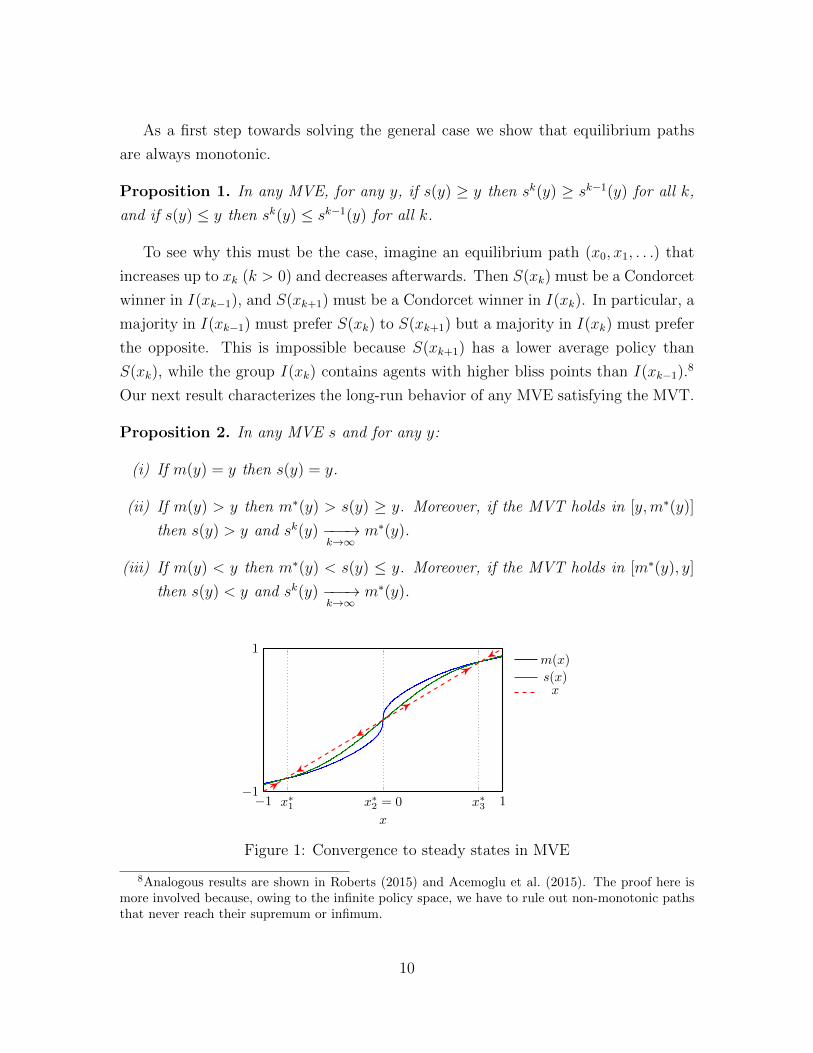
Proposition 2. In any MVE s and for any y:

(i) If m(y) = y then s(y) = y.

(ii) If m(y) > y then m∗(y) > s(y) ≥ y. Moreover, if the MVT holds in [y,m∗(y)]

then s(y) > y and sk(y) −−−→k→∞

m∗(y).

(iii) If m(y) < y then m∗(y) < s(y) ≤ y. Moreover, if the MVT holds in [m∗(y), y]

then s(y) < y and sk(y) −−−→k→∞

m∗(y).

−1 1−1

1

x∗1 x∗

2 = 0 x∗3

x

m(x)

s(x)x

Figure 1: Convergence to steady states in MVE

8Analogous results are shown in Roberts (2015) and Acemoglu et al. (2015). The proof here ismore involved because, owing to the infinite policy space, we have to rule out non-monotonic pathsthat never reach their supremum or infimum.

10

In other words, the steady states of any MVE s satisfying the MVT are simply the

fixed points of the mapping y 7→ m(y). Moreover, stable (unstable) steady states of

s are also stable (unstable) fixed points of m, and their basins of attraction coincide.

The intuition for why we should observe s(x) ≤ x if m(x) < x and vice versa

is straightforward: if m(x) < x for x in an interval (x∗, x∗∗), any policy in that

interval attracts a set of voters whose median wants a lower policy. The stronger part

of Proposition 2 is that slippery slope concerns cannot create myopically unstable

steady states—that is, s(x) 6= x if there is a myopic incentive to change the policy.

The logic behind the proof is as follows: suppose m(x) < x, but m(x) is afraid of

further policy changes if she moves to any y < x. If m(x) chooses a slightly better

policy y = x−ε, her flow payoff tomorrow will increase by roughly ε∣∣∂u∂x

∣∣. In exchange,

she will relinquish control over the continuation to a slightly different voter, m(x− ε).Because they have similar preferences (Assumption A2), m(x− ε)’s optimal choice is

also approximately optimal for m(x). Hence the cost of losing control is small, that

is, no higher than M(m(x) − m(x − ε))∑

t δk|sk(x) − sk(s(x − ε))|. If S(s(x − ε))

converges to S(x) pointwise as ε→ 0, this loss is of order o(ε), so m(x) should deviate

to y = x− ε for ε small enough. If not, it can be shown that m(x) must be indifferent

between S(x) and limε→0 S(s(x− ε)), and an analogous argument can then be made.

Figure 1 illustrates the equilibrium properties stated in Proposition 2 in an ex-

ample with three steady states: x∗1 and x∗3 are stable, while x∗2 is unstable. This

alternation of stable and unstable steady states occurs in general as long as m is

well-behaved. Formally, in the rest of the paper we will assume the following:

B1 The equation m(y) = y has finitely many solutions x∗1 < x∗2 < . . . < x∗N . In

addition, m′(x∗i ) 6= 1 for all i.

Corollary 1. m has an odd number of fixed points. For odd i, m′(x∗i ) < 1 and x∗i is

a stable steady state of every MVE; for even i, m′(x∗i ) > 1 and x∗i is unstable.

Our last result in this Section guarantees that, in a sizable neighborhood of each

stable steady state, every equilibrium must satisfy the MVT, and hence the full

version of Proposition 2. In addition, within the same neighborhood every equilibrium

must be monotonic (a stronger property than path-monotonicity) and an equilibrium

restricted to this neighborhood must exist.

11

Proposition 3. Let x∗ be such that m(x∗) = x∗ and m′(x∗) < 1; let x∗∗∗ < x∗ < x∗∗ be

the unstable steady states adjacent to x∗. Then an MVE restricted to I(x∗)∩(x∗∗∗, x∗∗)

exists, and any MVE is weakly increasing and satisfies the MVT in I(x∗)∩(x∗∗∗, x∗∗).

The reason these results may fail to hold outside of I(x∗)∩ (x∗∗∗, x∗∗) is that they

rely on pivotal voters not leaving the club on the equilibrium path; when pivotal

voters quit the club at different times, the logic that voters with higher bliss points

should like higher paths does not always apply.9

We finish this Section with two remarks. First, an alternative approach to solving

for MVEs would be to study a game in which, given a policy x, the agent m(x) is

by assumption given direct control over tomorrow’s policy.10 In this closely related

game, the full version of Proposition 2 holds for all Markov equilibria. Second, as

we will see next, under some conditions we will be able to guarantee the existence of

MVE that are monotonic and satisfy the full version of Proposition 2 everywhere.

4 Transition Dynamics

This Section analyzes the transition dynamics of the model in more detail. Without

loss of generality, we restrict our analysis to the right side of the basin of attraction of

a stable steady state, that is, an interval [x∗, x∗∗) such that m(x∗) = x∗, m(x∗∗) = x∗∗

and m(y) < y for all y ∈ (x∗, x∗∗).11

We begin by noting that, under mild conditions, convergence to a steady state

is far from instant, and becomes arbitrarily slow if agents are arbitrarily patient.

Formally, say m(x) ∈ (x∗, x∗∗) is reluctant if um(x)(x) > um(x)(x∗), i.e., m(x) would

rather stay at x than move instantly to x∗.12 If so, let z(x) be the unique policy below

m(x) for which um(x)(x) = um(x)(z(x)).

Proposition 4. If m(x) is reluctant, then, for all y < z(x), ∃K(y) > 0 such that, for

any δ and any MVE s of the game with discount factor δ, min{t : st(x) ≤ y} ≥ K(y)δ1−δ .

9For instance, let α = 0.6, α = 0.5, and S = (0.7, 0.1), T = (0.65, 0) be two-period policy paths.If α, α never leave under either path, Uα(S) − Uα(T ) > Uα(S) − Uα(T ) by A2; but if uα(0) < 0 itis possible that Uα(S)− Uα(T ) < Uα(S)− Uα(T ). By the same logic, the set of voters preferring Sto T may not be an interval, so a winning coalition need not contain the median voter.

10This approach has been taken in the literature, e.g., in Bai and Lagunoff (2011).11For any y ∈ (x∗, x∗∗), I(y) never wants to choose a policy outside of (x∗, x∗∗), so s|(x∗,x∗∗) can be

studied in isolation. Results for a basin of attraction of the form [x∗, 1] or [x∗∗∗, x∗] are analogous.12For instance, in the quadratic case, if m′(x) > 1

2 for all x then every agent is reluctant.

12

The reason is simply that, if this condition were violated, m(x) would rather stay

at x forever.13 Thus, if there are reluctant agents, knowing the club’s long-run policy

is not enough to characterize the agents’ utility even as δ → 1, unlike in related models

(cf. Acemoglu et al. 2012); further analysis of the transition path is necessary.

In the remainder of this Section we propose a natural class of equilibria, which

we call 1-equilibria (henceforth 1Es), and study their transition dynamics. There are

two reasons to focus on 1Es. The first is tractability: 1Es have a simple structure,

and their transition dynamics can be explicitly characterized in the limit as agents

become more patient. The second is robustness: 1Es are guaranteed to exist under

some conditions we will provide, while other types of equilibria (including smooth

equilibria) cannot be guaranteed to exist. We begin with a definition of 1Es and two

related concepts.

Definition 3. Let s be a successor function on [x∗, x∗∗]. s is a 1-function if there is

a sequence (xn)n∈Z such that xn+1 < xn for all n, xn −−−−→n→−∞

x∗∗, xn −−−→n→∞

x∗, and

s(x) = xn+1 if x ∈ [xn, xn−1). We call (xn)n the recognized sequence of s.

s is a 1-equilibrium (1E) if it is a 1-function and an MVE.

s is a quasi-1-equilibrium (Q1E) if it is a 1-function such that (1−δ)Um(xn)(S(xn+1)) =

um(xn)(xn+1) for all n.

x∗ x3x2 x1 x0

x

s(x)

m(x)

x

Figure 2: 1-equilibrium for uα(x) = C − (α− x)2, m(x) = 0.7x, δ = 0.7

In a 1E, the chosen policies are always elements of the recognized sequence (xn)n.

xn today leads to xn+1 tomorrow; if the initial policy is not part of the recognized

sequence, but is between xn and xn−1, then xn+1 is chosen, and the path follows the

13A partial converse holds: if um(x)(x∗) > um(x)(x) for all x then, for all y ∈ (x∗, x), min{t :

st(x) ≤ y} ≤ K(y), with K(y) independent of δ.

13

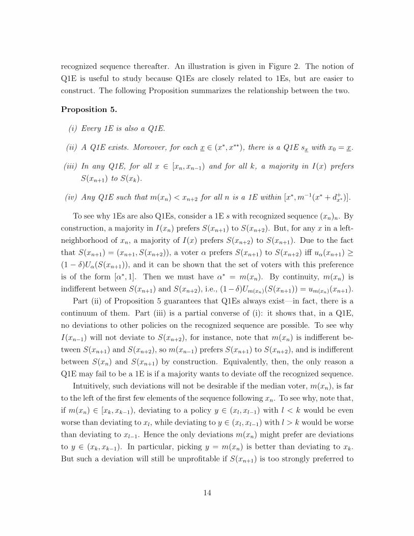
recognized sequence thereafter. An illustration is given in Figure 2. The notion of

Q1E is useful to study because Q1Es are closely related to 1Es, but are easier to

construct. The following Proposition summarizes the relationship between the two.

Proposition 5.

(i) Every 1E is also a Q1E.

(ii) A Q1E exists. Moreover, for each x ∈ (x∗, x∗∗), there is a Q1E sx with x0 = x.

(iii) In any Q1E, for all x ∈ [xn, xn−1) and for all k, a majority in I(x) prefers

S(xn+1) to S(xk).

(iv) Any Q1E such that m(xn) < xn+2 for all n is a 1E within [x∗,m−1(x∗ + d+x∗)].

To see why 1Es are also Q1Es, consider a 1E s with recognized sequence (xn)n. By

construction, a majority in I(xn) prefers S(xn+1) to S(xn+2). But, for any x in a left-

neighborhood of xn, a majority of I(x) prefers S(xn+2) to S(xn+1). Due to the fact

that S(xn+1) = (xn+1, S(xn+2)), a voter α prefers S(xn+1) to S(xn+2) iff uα(xn+1) ≥(1 − δ)Uα(S(xn+1)), and it can be shown that the set of voters with this preference

is of the form [α∗, 1]. Then we must have α∗ = m(xn). By continuity, m(xn) is

indifferent between S(xn+1) and S(xn+2), i.e., (1− δ)Um(xn)(S(xn+1)) = um(xn)(xn+1).

Part (ii) of Proposition 5 guarantees that Q1Es always exist—in fact, there is a

continuum of them. Part (iii) is a partial converse of (i): it shows that, in a Q1E,

no deviations to other policies on the recognized sequence are possible. To see why

I(xn−1) will not deviate to S(xn+2), for instance, note that m(xn) is indifferent be-

tween S(xn+1) and S(xn+2), so m(xn−1) prefers S(xn+1) to S(xn+2), and is indifferent

between S(xn) and S(xn+1) by construction. Equivalently, then, the only reason a

Q1E may fail to be a 1E is if a majority wants to deviate off the recognized sequence.

Intuitively, such deviations will not be desirable if the median voter, m(xn), is far

to the left of the first few elements of the sequence following xn. To see why, note that,

if m(xn) ∈ [xk, xk−1), deviating to a policy y ∈ (xl, xl−1) with l < k would be even

worse than deviating to xl, while deviating to y ∈ (xl, xl−1) with l > k would be worse

than deviating to xl−1. Hence the only deviations m(xn) might prefer are deviations

to y ∈ (xk, xk−1). In particular, picking y = m(xn) is better than deviating to xk.

But such a deviation will still be unprofitable if S(xn+1) is too strongly preferred to

14

S(xk). This is the idea behind part (iv); a more powerful result along these lines will

be given in the next subsection.

Finally, note that, in a 1E,m(xn)’s averaged per-period utility equals um(xn)(xn+1).

Hence her net gain from not staying at xn forever, V (m(xn)) := (1−δ)Um(xn)(S(xn+1))−um(xn)(xn), is approximately proportional to the equilibrium speed of policy change;

specifically, it equals (xn − xn+1)∣∣∣∂um(xn)(y)

∂y

∣∣∣ for some y ∈ [xn+1, xn].

Continuous Time Limit

We now characterize the limit of 1Es as the time gap between rounds of voting

becomes arbitrarily small. This can be taken as an approximation of a setting in which

voting happens periodically (e.g., at annual elections), but often enough relative to

the agents’ time horizon. The same results will also allow us to characterize the limit

of 1Es with a fixed time gap between periods as δ → 1.

Denote δ = e−r. We will work with the following objects. First, for each j ∈N, consider a version of the game from Section 2 in which policy and membership

decisions are made at every time t ∈ {0, 1j, 2j, . . .} instead of at every integer time. We

will call this the j-refined game, and denote a Q1E of this game by sj. In addition,

for each t ∈ R≥0, we denote by sj(x, t) the equilibrium policy at time t if the initial

policy is x and sj is played—that is, sj(x, t) = sbtjcj (x). Note that this game is, up to

a relabeling, equivalent to the model in Section 2 with discount factor δj = e−rj .

Finally, we define a continuous limit solution (CLS) as a function s(x, t) : [0,+∞)×[x∗, x∗∗)→ [x∗, x∗∗) with the following properties: s(x, t+ t′) ≡ s(s(x, t′), t); s(x, 0) ≡x; s is weakly decreasing in t; s(x, t) −−→

t→0x for all x; and Um(x)(S(x)) = um(x)(x) for

all x ∈ (x∗, x∗∗), where Uα(S(x)) =�∞

0re−rt max(uα(s(x, t)), 0)dt.

The following Proposition relates the CLS to the Q1Es of the j-refined games.

Proposition 6. Suppose that m ∈ C2 and a CLS s exists. Then:

(i) s is the unique CLS, and s is C1 as a function of t.

(ii) For any sequence (sj)j, where sj is a Q1E of the j-refined game, for all x and

t, sj(x, t) −−−→j→∞

s(x, t).

(iii) There is δ < 1 such that, for all δ > δ, all Q1Es of the discrete-time game with

discount factor δ are 1Es.

15

The intuition behind a CLS is the following. Fix x, and take a sequence (sj)j

of Q1Es of the j-refined games with xj0 = x. Recall that Um(xjn)(Sj(xj(n+1))) =

um(xjn)(xj(n+1)) for all j, n.14 Suppose that, as j →∞, the transition paths Sj(x) =

(sj(x, t))t converge pointwise to a continuous path S(x). Then differences xj0 − xj1go to zero, and in the limit, Um(x)(S(x)) = um(x)(x). This is why we require this

condition of a CLS. Part (ii) of Proposition 6 is a converse to this argument: it shows

that, when a CLS exists, the transition paths of all Q1Es must converge to it as

j →∞.

Whether a CLS exists is a property of the primitives u and m; it can be determined

in isolation from our game. We can both verify whether a CLS exists and calculate it

explicitly, as follows. Denote by e(x) = − 1∂s(x,t)∂t|t=0

the instantaneous delay of a CLS

at x. If Um(x)(S(x)) = um(x)(x) for all x, then, differentiating with respect to x,

m′(x)∂Um(x)(S(x))

∂α= m′(x)

∂um(x)(x)

∂α+∂um(x)(x)

∂x. (1)

The key observation is that ∂∂x

∂Um(S(x))∂α

=(∂um(x)(x)

∂α− ∂Um(S(x))

∂α

)re(x). Hence, differ-

entiating Equation 1 yields an equation that pins down e(x). After rearranging, we

find

−∂u∂xre(x) = 2m′

∂2u

∂α∂x+∂2u

∂x2+ (m′)2

(∂2u

∂α2− ∂2Um(x)(S(x))

∂α2

)− m′′

m′∂u

∂x, (2)

where u stands for um(x)(x). This is an integral equation because ∂2U∂α2 is evaluated at

S(x), which depends on e(y) for y ∈ [x∗, x). But we can solve it forward, starting

at x∗, to find e(x) and, with it, the unique CLS. In fact, a CLS always exists unless

the function e(x) that solves Equation 2 turns negative. This is guaranteed not to

happen if the forces pulling towards policy change are not too great:

Proposition 7. Holding u constant, there exist B, B′, B′′ > 0 such that, if x−m(x) ≤B, m′(x) ∈ [1−B′, 1 +B′] and m′′(x) ≥ −B′′ for all x, then a CLS exists.

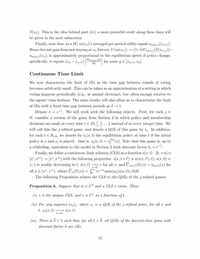
The quadratic case is useful for illustrative purposes. In that case, for x ∈ I(x∗),

Equation 2 reduces to

re(x) =2m′(x)− 1

x−m(x)+m′′(x)

m′(x), (3)

14In this argument, we write Um(x)((xt)t) = (1− δ)∑ δtIαtuα(xt) to simplify notation.

16

x∗

xs(x, 1)

m(x)

e(x)

x

Figure 3: A continuous limit solution

so the speed of convergence can be calculated in closed form. Equation 3 reflects

three forces at work in determining e(x). First, the policy changes more slowly (e(x)

is higher) when the myopic incentive for policy changes, x−m(x), is small. Second,

the policy changes more slowly when m′(x) is high. The reason is that changing the

policy to x−ε entails yielding control to another agent m(x−ε). The higher m′ is, the

more costly this loss of control becomes. Third, the policy changes more slowly when

m′′(x) is high. The reason is that, when m is convex, m′(x) is higher than m′(x− ε);hence the agent m(x) yields control to will not be as concerned about the behavior

of her own successors, and so will make faster policy changes than m(x) would like.

These forces are illustrated in Figure 3.

Finally, part (iii) of Proposition 6 guarantees that, when there is a CLS, all Q1Es

must be true 1Es when agents are patient enough. The reason is related to our

discussion of Proposition 5: as the transition paths of Q1Es approach the CLS, they

must feature smaller and smaller jumps between consecutive policies; in this scenario,

deviations off the recognized sequence are never majority-preferred.

We conclude this Section with a few observations. First, the speed of policy change

in a CLS is exactly inversely proportional to the agents’ patience:

Remark 1. If s(x, t) is a CLS for discount rate r, then s(x, t) ≡ s(x, r

rt)

is a CLS for

discount rate r. The respective instantaneous delays e(x), e(x) satisfy e(x) = rre(x).

The reason is that changing r is equivalent to a relabeling of the time variable.

Second, when a CLS exists, Proposition 6 and Equation 2 together yield an asymptotic

characterization of the transition path for all 1Es of the game from Section 2 when

17

agents are patient.15 Formally, let e1(x) be the solution to Equation 2 for r = 1.

Then, for any y < x and any collection of 1Es sδ for δ ≥ δ,

(1− δ) min{t : stδ(x) ≤ y} −−→δ→1

� x

y

e1(z)dz. (4)

This is, in effect, a more precise version of Proposition 4. Third, recall that, in a

1E, the net per-period gain V (m(xn)) of a pivotal agent m(xn) from following the

equilibrium path (relative to staying at xn) is of the order xn− xn+1. Thus, if a CLS

exists, for any x and any collection of 1Es sδ, Vδ(m(x))→ 0 as δ → 1. In other words,

the “rents” a pivotal agent gets from the best non-constant continuation evaporate

as agents become more patient (or decisions are made more often). An intuition is

that these rents are the result of agents being able to “lock in” their chosen policy

for one period before losing control—hence they vanish as the periods shorten.

Fourth, it is not hard to find examples in which a CLS fails to exist.16 However,

even when there is no CLS, a version of Proposition 6 holds: under some conditions,

Q1Es can still be guaranteed to be 1Es for high δ, and all sequences of Q1E transition

paths converge to a common limit, but this limit is no longer continuous. The details

for this case are presented in Appendix B.

5 A Model of Political Power

We now discuss a variant of the model that overturns the assumption of free entry

and exit. Consider a polity governed by an endogenous ruling coalition. At each time

t = 1, 2, . . . the ruling coalition chooses a policy xt; the initial policy x0 is exogenous.

The model is the same as the one presented in Section 2, but with two differences.

First, the policy xt now directly determines not just the flow payoffs of all agents

during the period [t, t+ 1), but also the ruling coalition at time t+ 1. In other words,

the mapping x 7→ I(x) is now taken as a primitive of the model. (We assume that

I(x) is still an interval (x− d−x , x+ d+x ) for each x, with x− d−x , x+ d+

x increasing and

C1 as functions of x.) Second, in this model, all agents are impacted by the policy,

15This is a consequence of Proposition 6 for a sequence (δj)j of the form δj = e−rj , but in fact the

proof of the Proposition does not rely on the j’s being integers, only that j →∞.16For example, if there is a non-reluctant agent, then a CLS cannot exist.

18

regardless of whether they are in the ruling coalition. In other words,

Uα ((xt)t, Iα) =∞∑t=0

δtuα(xt),

where uα satisfies A1, A2 and A4. This setting is similar to the canonical model of

“elite clubs” (Roberts, 2015), but with a continuous policy space. It can be framed

as a model of enfranchisement (Jack and Lagunoff, 2006), institutional change (Ace-

moglu et al., 2012, 2015), or economic policymaking in a world where political influ-

ence is a function of wealth (Bai and Lagunoff, 2011). Clearly, slippery slope concerns

apply here as well: a ruling coalition may want to expand the franchise (e.g., to lower

unrest) but fear that the new voters will choose to expand it even further.

Our analysis of the main model extends to this case as follows. First, all of our

previous Propositions continue to hold, with analogous proofs. Second, Propositions

3 and 5(iv) now hold everywhere, as opposed to only within a neighborhood of each

stable steady state.17 In particular, an MVE exists; every MVE satisfies the MVT

everywhere; and for every MVE sk(x) −−−→k→∞

m∗(x) for all x.

Although this version of the model represents a setting with different causal rela-

tionships between political power, membership, and flow payoffs, it is closely related

to the model from Section 2: indeed, there is a mechanical equivalence between the

components of both models, and the same tension between current payoffs and future

control is present in both cases.

Other variants, allowing the model to fit new examples, are possible. For instance,

the set of members can affect payoffs directly: vα(x) = uα(x) + wα(I(x)). So long as

vα(x) satisfies A1-4, all of our results apply. A natural example is immigration: if xt

is a country’s immigration policy and I(xt) is its set of citizens, xt does not affect the

payoffs of current citizens directly, but the entry of immigrants does.18

6 Discussion

This Section discusses some implications of our analysis.

17The proofs of Propositions 3 and 5(iv) only go through when pivotal agents never stop receivingpayoffs from the club’s policy. In the main model, this requires them not to leave the club; in thisvariant it does not matter if they are part of the ruling coalition.

18This example has been studied in the literature, although in an overlapping-generations frame-work (Ortega, 2005; Suwankiri, Razin and Sadka, 2016).

19

Myopic Stability of Steady States

Two central results of our analysis are that steady states are myopically stable (or, in

the language of Roberts (2015), “extrinsic”),19 and convergence to a steady state is

slow when agents are patient. In contrast, in other papers in this literature (Roberts,

2015; Acemoglu et al., 2008, 2012, 2015), intrinsic steady states are possible, and the

time it takes to converge to a steady state is uniformly bounded even as δ → 1.

These papers assume a fixed, finite policy space. Under this assumption, conver-

gence is fast because there is a mechanical lower bound on the size of policy changes;

as a result, intrinsic steady states must exist for δ high enough, if there are reluctant

agents. What we show is that these results are overturned if arbitrarily small policy

changes are allowed. For a fixed δ < 1, our results also hold if the policy space is

finite but fine enough; if we simultaneously take δ to 1 and make the policy space

arbitrarily fine, whether intrinsic steady states exist depends on the order of limits.

The upshot is that, in practice, whether dynamic concerns can indefinitely stall

policy changes depends not just on the agents’ foresight but also on institutional

details that determine whether incremental changes are possible. For example, take

a polity with a limited franchise considering a franchise extension on the basis of

income. Suppose that each voter prefers a larger franchise than the smallest one she

would be in (e.g., for all x, a voter at the xth income percentile wants to enfranchise

everyone above the (x− 5)th percentile). Then, if it is possible to enfranchise the top

y% of the income distribution for any y, full democracy would eventually be reached

through a series of small changes. However, if voting rights can only be extended

based on a few criteria (e.g., only to men who can read, to landowners, to taxpayers,

etc.), indefinite stalling is likely.20

Two important precursors to our analysis, Jack and Lagunoff (2006) and Bai and

Lagunoff (2011), consider dynamic political decision-making with continuous policy

spaces. In particular, Bai and Lagunoff (2011) show that in their model, steady states

of “smooth” equilibria are also stable when the current decision-maker is assumed to

retain power forever (in our setting, this is equivalent to myopic stability). However,

their analysis uses a first-order approach, and so does not extend to other types of

equilibria; moreover, smooth equilibria generically fail to exist, as the second-order

19This is true for all 1Es; for all other MVEs in a neighborhood of each stable steady state; andglobally for all MVEs in the model discussed in Section 5, which is closest to this literature.

20Jack and Lagunoff (2006) make the case that franchise extensions are typically gradual processes.

20

conditions are typically violated.21 We build on this result by showing that steady

states must be myopically stable for all equilibria, including discontinuous ones.

Distribution of Steady States

Although f is the primitive of our model describing the distribution of preferences,

our results are best stated in terms of m, the median voter function. Here, we briefly

discuss the relationship between the two objects, focusing on how the shape of f

affects the location of steady states.

In the quadratic case, or more generally whenever I(x) ≡ (x−d, x+d) is symmetric

around x, the distribution of steady states reflects the following intuition: if f is

increasing within I(x) then m(x) > x, and vice versa. Hence, stable steady states

correspond roughly to maxima of the density function.

Remark 2. If I(x) = (x−d, x+d) for all x, and x∗ is a stable (unstable) steady state,

then I(x∗) contains a local maximum (minimum) of f .

In particular, if f is increasing (decreasing) everywhere, there is a unique steady

state close to 1 (−1); if f is symmetric and single-peaked, 0 is the unique steady state.

Thus, the organization always moves to the center if the distribution of preferences

is bell-shaped. Yet, there are three scenarios in which the organization may converge

to a policy more extreme than the bliss points of most voters.

First, even if most voters are near the center, a local maximum near an extreme

may support a stable steady state, especially if d is low.22

Remark 3. If f ′(x∗) = 0 and f ′′(x∗) < 0, then there is d > 0 such that for all d < d,

if I(x) ≡ (x− d, x+ d) for all x, (x∗ − d, x∗ + d) contains a stable steady state.

Second, even if there is a unique steady state, its location will be unstable when f is

close to uniform. For example, consider the densities f1(x) = 12+εx, f2(x) = 1

2−εx and

f3(x) = 1+ε2−ε|x|, for a small ε > 0. These are all close to each other (||fi−fj||∞ ≤ 2ε

∀i, j) but f1 has a unique steady state near −1, f2 has one near 1, and f3 has one at

0. Hence, the long-run policy is potentially discontinuous in f , unlike in models of

voting with a fixed population.

21The existence properties of smooth equilibria are discussed in Appendix D.22Note that, when there are multiple steady states, which one the organization converges to de-

pends on the initial policy, i.e., there is path-dependence. There is no guarantee that the organizationwill converge to a steady state that attracts the most members or maximizes aggregate welfare.

21

Third, the tendency towards policies preferred by a majority can be easily over-

turned when the voter sets I(x) are not symmetric around x. In particular, if agents

with extreme preferences are disproportionately more willing to join the organization,

they can capture it despite being a minority, even locally.23

For example, let the policy space be [−1, 1], where −1 is the most moderate policy

and 1 the most extreme, and assume uα(x) = −|α− x|+ (1 + α).24 Then α wants to

be a member whenever x ∈ [−1, 2α + 1], whence I(x) = [−1+x2, 1].

Suppose f is as follows: moderates constitute 60% of the population and have bliss

points uniformly distributed in [-1,-0.9]; extremists, the remaining 40%, have bliss

points uniformly distributed in [-0.9,1]. It can then be shown that the unique steady

state is x∗ = 13> 0. At the steady state policy, the set of members I(1

3) = [−1

3, 1] is

only 28% of the population, all of them extremists.

7 Conclusion

We conclude with a discussion of some issues that the model leaves out, possible

extensions, and additional results presented in the Appendix.

Our model focuses on the behavior of a single organization, but organizations

often compete—in particular, the usual assumption in Tiebout competition is that

there are many districts. There are two ways of modeling competition. The first is

to assume, as in the idealized Tiebout model, that districts are identical except for

their policies. In such a model, the same dynamics we have studied would arise, but

with the complication that policy changes in one district may lead to responses by

other districts. At the same time, if there are enough districts, every agent would

find a district near her bliss point, so the potential welfare impact of policy changes

in individual districts would vanish as the number of districts grows.25

An alternative approach is to assume that districts are imperfect substitutes. The

example in Section 2 of a city with a competitive advantage over others is a version

of this, and it can be generalized. Suppose that there are k > 1 special cities c∗1,

23This asymmetry is likely in settings where too-extreme policies are perceived as reprehensible orcriminal, but not the reverse (e.g., fringe political parties, violent protest movements, or advocacygroups whose causes can be perceived as racist or xenophobic).

24The example is degenerate in that ∂2u∂α∂x is only weakly positive and u is only weakly concave in

x; this is only for simplicity.25Tiebout (1956) conjectured that agents sorting into compatible districts would lead to an efficient

outcome. This idea has been formalized (Wooders, 1989) as well as criticized (Bewley, 1981).

22

. . ., c∗k and k groups of mobile agents, so that agent types are of the form (α, i), for

i ∈ {1, . . . , k}, and group i’s bliss points are distributed according to a density fi.

Assume that u(α,i)(c) = C1c=c∗i − (xt(c) − α)2, that is, agents in group i only value

the city c∗i more than normal cities. (For instance, agents in group i have immobile

relatives in city i.) Our analysis goes through because each special city c∗i competes

only for agents in group i, and does so only with normal cities. If i’s value from

c∗j 6= c∗i is some intermediate C ′ ∈ (0, C), the problem becomes more complicated,

but the relevance of the forces we study does not vanish as k →∞. Thus, our model

can be taken as an analysis of Tiebout competition in the presence of imperfect

substitutability. A similar logic would apply if cities are ex ante identical but have

ex post market power due to moving costs.26

A related extension would allow for the endogenous creation of organizations.

Our analysis suggests that an agent far from a steady state is less likely to create an

organization, or more likely to create a non-democratic one.

The organizations we model are simple: all members have the same voting power,

decisions are made by majority rule, and votes are cast independently. Appendix E.1

discusses how to extend our analysis to allow for supermajority rules or other electoral

rules that make an agent other than the median pivotal.27 However, there is much

unexplored complexity regarding the internal structure of organizations. Agents may

have endogenous voting power (seniority); or they may engage in collective behavior

by voting as a bloc, joining an organization in large numbers in order to change its

policy, or threatening to leave en masse to extract concessions. These behaviors are

not likely in the context of Tiebout competition, but may be so in other applications.

Organizations may also set up various barriers to entry or membership restrictions

(or, in the case of cities, there may be moving costs). In the paper, we consider two

extreme cases: one with completely free entry and exit (Section 2) and one in which

the organization can choose its set of members at will (Section 5). In Appendix

E.2, we present an extension allowing for (exogenous) positive entry and exit costs.

Because in equilibrium agents enter and leave the organization at most once, this

does not change the analysis much. Modeling endogenous entry costs that can be

chosen separately from the organization’s main policy, on the other hand, is much

26Moving costs and idiosyncratic preferences are suggested in Tiebout (1956) and Epple and Romer(1991), respectively, as forces preventing convergence to a Tiebout equilibrium in practice.

27Even in democracies, higher-income agents may wield more political power (Benabou, 2000;Jack and Lagunoff, 2006).

23

harder, as the state space becomes multidimensional. However, the forces we study

will still be present as long as the organization cannot perfectly control both its

payoff-relevant policy and its membership (if it can, we are back in the world of a

fixed decision-maker).

Our analysis abstracts away from history-dependent strategies by focusing on

Markovian equilibria. In Appendix E.3, we show that Non-Markovian equilibria can

support a large number of outcomes, but that several reasonable refinements select

only Markovian equilibria. In particular, any equilibrium obtainable as a limit of

discrete policy-space equilibria must be Markovian.

Finally, we do not explicitly model the organization’s voting process. One way

to interpret our results is that they will hold whenever the organization’s collective

decision-making process leads to Condorcet-winning policies being chosen. In Ap-

pendix E.4, we discuss possible microfoundations of this modeling assumption. In

particular, the MVEs we study are Markov Perfect Equilibria of a game in which, in

each round of voting, there are two short-lived, office-motivated candidates engaging

in Downsian competition. However, not all political processes are so well-behaved.

For instance, if the organization has more than two candidates running for office, or

it is run by a deliberative decision-making process, then the Condorcet winner may

not win.28 In addition, leaders typically have some agency in practice. If they are

long-lived and have heterogeneous appeal, or are policy-motivated, they may cham-

pion certain policies in an attempt to change the policy path, possibly permanently.

Moreover, a politician may strategically push for policies that will attract a set of

members predisposed to like her.29

Appendices B, C and D contain technical results. Appendix B contains the proofs

of Propositions 6 and 7 and characterizes the case in which no CLS exists. Appendix

C shows that the limit solution described in Appendix B exists for all m satisfying

a genericity condition. Appendix D discusses the existence properties of equilibria

other than 1Es (in particular, smooth equilibria and k-equilibria, a generalization of

1Es); calculates explicit equilibria for the case of linear m and quadratic utility; and

gives an example of an MVE that is non-monotonic outside of I(x∗).

28For example, Bouton and Gratton (2015) shows that Condorcet winners may lose in majorityrunoff elections with three candidates.

29Glaeser and Shleifer (2005) discusses the case of Mayor Curley of Boston, who used wastefulpolicies in an effort drive out rich citizens of English descent, as he was most popular among thepoor Irish population.

24

A Proofs

Lemma 2. Let S = (x0, x1, . . .), T = (y0, y1, . . .) be two policy paths, and let I(S) =

∪∞n=0I(xn), I(T ) = ∪∞n=0I(yn). Suppose that supxn < inf yn; I(S), I(T ) are intervals;

and I(S) ∩ I(T ) 6= ∅. Then there is α0 such that agents in [−1, α0) strictly prefer S

to T , and agents in (α0, 1] strictly prefer T to S.

Proof. Let x = inf xn, x = supxn, y = inf yn, y = sup yn. By assumption, x ≤ x <

y ≤ y. Note that all agents α < x strictly prefer S to T by A4 and A6; likewise, all

α > y strictly prefer T to S.

Let W (α) = Uα(T )− Uα(S). Note that W is continuous and W (x) < 0 < W (y).

Hence there is some α0 ∈ [x, y] for which W (α0) = 0. For any α ∈ [x, y], let

I−S (α) =∑∞

n=0 δn1xn≤α,uα(xn)>0, I+

S (α) =∑∞

n=0 δn1xn>α,uα(xn)>0. Define I−T (α), I+

T (α)

analogously.

If α ∈ [x, y], then I−S (α) ≥ I−T (α) = 0 = I+S (α) ≤ I+

T (α), and I−S (α) + I+T (α) > 0

by the assumption that I(S) ∩ I(T ) 6= ∅. Then W ′(α) > 0 by A5.

If α ∈ [y, y], then I+S (α) = 0, and one of the following must be true. If I−S (α) ≤

I−T (α), then W (α) > 0 by A4, and moreover W (α′) > 0 for all α′ ∈ [α, y]. If

I−S (α) > I−T (α), then W ′(α) > 0 by A2 and A5. Similarly, for each α ∈ [x, x], either

W ′(α) > 0 or W (α′) < 0 for all α′ ∈ [x, α].

In general, then, we can find thresholds z0, z1 such that x ≤ z0 ≤ x < y ≤ z1 ≤ y;

W ′(α) > 0 for all α ∈ [z0, z1]; W (α) < 0 for all α ∈ [x, z0); and W (α) > 0 for all

α ∈ (z1, y]. Hence W can vanish at most at one point, so α0 is unique.

Lemma 3. In any MVE s, for any y, I(y) ∩ I(s(y)) has positive measure. Hence

I(S(y)) is an interval for all y.

Proof. Suppose WLOG y < s(y). We argue that y + d+y > s(y)− d−s(y). Suppose this

is false; then all voters in I(y) get utility 0 from policy s(y). If E = {α ∈ I(y) :

Uα(S(s(y))) > 0} is a strict majority of I(y), this leads to a contradiction, as all of

E would strictly prefer S(s2(y)) to S(s(y)). Let D = {α ∈ I(y) : Uα(S(s(y))) ≥Uα(S(y))} ⊆ E. Since S(s(y)) is a Condorcet winner in I(y), D is a majority in

I(y). If I(y) ⊆ D we are done. If not, ∃α0 ∈ I(y) − D. By the continuity of

Uα(S(s(y))), ∃α1 such that 0 < Uα1(S(s(y))) < Uα1(S(y)), and this inequality holds

in some neighborhood (α1 − ε, α1 + ε). Hence E −D has positive measure and E is

a strict majority of I(y).

25

Corollary 2. In any MVE, let S = S(y) for some y < x and T = (x, x, . . .), with

sup(S) ≤ x. Then there is α0 ≤ x such that agents in [−1, α0) strictly prefer S to T ,

and agents in (α0, 1] strictly prefer T to S.

Proof. If I(S)∩ I(x) 6= ∅, this follows directly from Lemmas 2 and 3. If not, then all

α ≥ x− d−x strictly prefer T to S and all α ≤ sup I(S) strictly prefer S to T . Let α′0

be such that uα′0(y) = uα′0(x) < 0. If α′0 ∈ (sup I(S), x − d−x ) then take α0 = α′0. If

α′0 ≤ sup I(S) then take α0 = I(S). If α′0 ≥ x− d−x take α0 = x− d−x .

Proof of Proposition 1. Suppose S(y) is not monotonic. For this proof, denote sk =

sk(y), Sk = S(sk), Ik = I(sk), y = inf(S(y)) and y = sup(S(y)). For brevity, we will

say α prefers a policy x to a path S if she prefers (x, x, . . .) to S. There are two cases:

Case 1: S(y) attains y or y, i.e., ∃k ∈ N such that sk = y or sk = y. Suppose

WLOG the former. Then there is a k ∈ N such that sk−1 < y, sk = y and sk+1 < y.30

Consider the decision made by voters in Ik−1 and in Ik. Since Sk is the Condorcet

winner in Ik−1, a majority of Ik−1 prefer it to Sk+1. At the same time, Sk+1 is

Condorcet-winning in Ik, so a majority of Ik prefer Sk+1 to Sk. Let A = (sk−1 −d−k−1, sk − d−k ), B = (sk − d−k , sk−1 + d+

k−1), C = (sk−1 + d+k−1, sk + d−k ). Note that α

prefers Sk to Sk+1 iff he prefers sk to Sk+1. Apply Corollary 2. If α0 ∈ C, all voters

in A∪B strictly prefer Sk+1 to Sk, a contradiction. If α0 ∈ B, all voters in A strictly

prefer Sk+1 to Sk and all voters in C strictly prefer Sk to Sk+1, a contradiction.

Case 2: S(y) never attains its infimum nor its supremum. Then there must be a

subsequence (ski)i such that ski −→i→∞

y. Construct a sub-subsequence skij such that

skij −→j→∞ y and skij−1 −→j→∞

s−1∗ for some limit s−1

∗ ≤ y. (We can do this because

all the sk are in [−1, 1], which is compact.) Iterating this, construct a nested list of

subsequences ((skim)i)m such that kim is increasing in i for each m; Km = {kim : i ≥0} ⊇ Km′ for m < m′; and, for each m, skim+r −→

i→∞sr∗ for any r ∈ {−m, . . . ,m}, where

s0∗ = y. Let gi = kii. Then (sgi)i is a subsequence of (sk)k such that sgi+r −→

i→∞sr∗ for

any r ∈ Z. We now consider four sub-cases.

Case 2.1: Suppose sr∗ < y for some r < 0 and for some r′ > 0, and let r < 0 < r be

the numbers closest to 0 satisfying these conditions. Consider the decisions made by

Igi+r and Igi+r−1, for high i. In the limit, they imply that a majority in I(sr∗) prefers y

to S(sr∗), while a majority in I(y) prefers S(sr∗) to y (denoting S(sr∗) = (sr∗, sr+1∗ , . . .)).

As in Case 1, this contradicts Corollary 2.

30The same argument would apply if sk(y) = . . . = sk+m(y) > sk−1(y), sk+m+1(y).

26

Case 2.2: Suppose sr∗ < y for some r < 0 but never for r > 0. Take r maximal, so

sr∗ < y and sr∗ = y ∀r > r. Fix 0 < ν < y−sr∗. For each i, let r′(i) be such that sgi+r′(i)

is the first element of the sequence (sk)k after sgi+r that is weakly smaller than sr∗+ν.

Construct a subsequence (sgij )j such that sgij+r′(ij)+l → sl∗∗ for l ≥ −1 (in particular

s−1∗∗ ≥ sr∗ + ν ≥ s0

∗∗). Now compare the decisions made by I(sgi+r) and I(sgi+r′(i)−1).

In the limit, they imply that a weak majority in I(sr∗) prefers y to S(s0∗∗), while a weak

majority in I(s−1∗∗ ) prefers the opposite (here S(s0

∗∗) = (s0∗∗, s

1∗∗, . . .)). This contradicts

Corollary 2.

Case 2.3: Suppose sr∗ < y for some r > 0 but never for r < 0. Take r minimal, so

sr∗ < y and sr∗ = y ∀r < r. Fix 0 < ν < y − sr∗. Let r′ν(i) be such that sgi+r′ν(i) is the

last element before sgi that is weakly smaller than y − ν. Clearly r′ν(i) −→i→∞−∞.

Consider the choice made by I(sgi+r−1). In the limit, a majority in I(y) prefers

(sr∗, sr+1∗ , . . .) over y. Apply Corollary 2. Clearly α0 < y, so m(y) ≤ α0 < y. As

m is strictly increasing, mk(y) is strictly decreasing in k and converges to a limit m;

moreover, m(y) < y for all y ∈ (m, y]. Call gi+r′ν(i) = hiν and let sν∗ = lim infi→∞ shiν .

Let s∗∗ = lim infν→0 sν∗. If s∗∗ < y, take a sequence of ν, hiν such that shiν → s∗∗. By

construction shiν+l ≥ y−ν for l = 1, . . . , L for L arbitrarily large as ν → 0, hiν →∞.

Then, in the limit, y is a Condorcet winner in I(s∗∗); in particular, a majority prefers

y to (sr∗, sr+1∗ , . . .), which contradicts Corollary 2.

If s∗∗ = y we must work away from the limit. Take ε > 0 such that (y−d−y +ε, y−ε) ⊆ I(y − υ) is a strict majority of I(y − υ) for all 0 < υ ≤ ε.31 Take a fixed ν ′ < ε;

a ν < ν ′ such that sν∗ ≥ y − ν ′; and a subsequence sfi of shiν such that sfi → sν∗. Let

Mi be the largest integer such that sfi+l ∈ (y − ν, y) for l = 1, . . . ,Mi and Ki the

set of l ∈ 1, . . . ,Mi such that sfi+l ∈ (y − ν2, y). Let ki = min(Ki). By construction,

Mi, |Ki| → ∞. Then, for α ∈ (y − d−y + ε, y − ε),

1

1− δuα(sfi)− Uα(S(sfi+1)) =∑t∈Ki

δt−1 (uα(sfi)− uα(sfi+t)) +

+∑

Mi≥t/∈Ki

δt−1 (uα(sfi)− uα(sfi+t)) +∑t>Mi

δt−1(uα(sfi)− 1α∈I(sfi+t)uα(sfi+t)

)≥ δki−1 (uα(sfi)− uα(sfi+ki)) + 0− δMi

1− δC = δki−1

(uα(sfi)− uα(sfi+ki)−

δ|Ki|

1− δC)

where C = maxα uα(α). Note that uα(sfi) − uα(sfi+ki) ≥ usfi (sfi) − usfi (sfi+ki) +

31ε exists because m(y) < y and y − d−y , y + d+y are continuous in y.

27

M ′(sfi − α)(sfi+ki − sfi) ≥ M ′(sfi − y + ε)ν2, which converges to M ′(sν∗ − y + ε)ν

2≥

M ′ ν2(ε − ν ′) > 0 as i → ∞. On the other hand, δ|Ki| → 0 as i → ∞. Hence all

α ∈ (y− d−y + ε, y− ε) prefer sfi to S(sfi+1) for high i, so S(sfi+1) is not a Condorcet

winner in I(sfi), a contradiction.

Case 2.4: sr∗ = y for all r. In other words, the sequence spends arbitrarily long

times near y and y (if not true for both boundaries, one of the former cases applies).

We first prove the following claim: m(y) = y for all y ∈ [y, y].

Take any y0 ∈ (y, y). Take a sequence (hi)i such that, for each i, shi is the last

element of the sequence (sk)k before sgi such that sk ≤ y0. Intuitively, shi is the last

element of the sequence below y0 before the sequence goes near y for a long time.

Take a diagonal subsequence (ski) of (shi) such that ski+l has a limit sl∗∗ for all i.

Clearly s0∗∗ ≤ y0 and sl∗∗ ≥ y0 for all l > 0.

Consider the choice made by I(ski). If s0∗∗ < y0, in the limit, a majority in I(s0

∗∗)

prefers (s1∗∗, s

2∗∗, . . .) over s0

∗∗. Apply Corollary 2. Clearly m(s0∗∗) ≥ α0 > s0

∗∗, so

um(s0∗∗)(s0∗∗) ≤ um(s0∗∗)(y0). If s0

∗∗ = y0, then m(y0) < y0 leads to a contradiction by

an analogous argument as in Case 2.3, so we must have m(y0) ≥ y0. Conversely,

considering sequences going near y for arbitrarily long, we obtain that either m(y0) ≤y0 or there is s0

∗∗ > y0 such that m(s0∗∗) < s0

∗∗ and um(s0∗∗)(s0∗∗) ≤ um(s0∗∗)(y0).

For each y ∈ (y, y) such that y 6= m(y), define y 6= y to be such that um(y)(y) =

um(y)(y). Take y0 such that |y0 − y0| is maximal. WLOG m(y0) < y0, so there is

s0∗∗ < y0 such that m(s0

∗∗) > s0∗∗ and um(s0∗∗)(s

0∗∗) ≤ um(s0∗∗)(y0). Since m(y0) > m(s0

∗∗),

um(y0)(s0∗∗) < um(y0)(y0), so y0 > s0

∗∗; but s0∗∗ ≥ y0. Hence |s0

∗∗ − s0∗∗| > |y0 − y0|, a

contradiction.

For the case where m(y) = y for all y ∈ [y, y], we use the following Lemma.

Lemma 4. Let S = (y, y, . . .), and let T = (xn)n 6= S. If x and x′ both prefer T to

S, and x < y < x′, then x /∈ I(x′) or x′ /∈ I(x).

Proof. Suppose for that x ∈ I(x′) and x′ ∈ I(x). It is enough to check the case where

T is contained in [x, x′]: if not, define a path (xn)n by xn = min(max(xn, x), x′). Then

(xn)n is contained in [x, x′] and is weakly better for both x and x′ than T .

By assumption, both x and x′ derive non-negative utility from all elements of T .

Let x = (1 − δ)∑

n δnxn, and T ′′ = (x, x, . . .). If T ′′ 6= T , both x and x′ strictly

prefer T ′′ to T by Jensen’s inequality and A4. Hence they both strictly prefer x to y,

a contradiction. If T ′′ = T , x 6= y and both agents prefer x to y, a contradiction.

28

Take ε > 0, ν > 0 small and y0 = y + ε. Construct ski as before. It follows

from previous arguments that s0∗∗ = y0. For all i, a majority in I(ski) must prefer

S(ski+1) over ski . Since ski strictly prefers ski over S(ski+1) and ski = m(ski), this

can only happen if there are voters both above and below ski who prefer S(ski+1).

Let y′i < ski < y′′i be the closest voters to ski who weakly prefer S(ski+1), and denote

y′i−(ski−d−ski ) = η′i, y′′i −ski = η′′i . Note that η′i, η

′′i −→i→∞

0.32 In addition, y′′i −d−y′′i > y′i;

otherwise we obtain a contradiction as in Lemma 4. Let yi be such that yi− d−yi = y′i.

Given the path T i = S(ski+1) construct T ′i as follows. If T ij ≥ y′′i +ν, T ′ij = y′′i +ν.

If y′′i + ν > T ij ≥ yi, T′ij = y′′i . If yi > T ij ≥ ski , T

′ij = zi =

∑yi>T

ij≥ski

δjT ij∑yi>T

ij≥ski

δj. If

ski > T ij , T′ij = vi =

∑ski

>TijδjT ij∑

ski>Ti

jδj

. Then both y′i and y′′i weakly prefer T ′i over T i.

Moreover, T ′i is a linear combination of at most four policies; by an abuse of notation,

T ′i = ωi1[y′′i ] + ωi2[y′′i + ν] + ωi3[zi] + ωi4[vi] with∑

j ωij = 1. In addition, since S(ski+1)

spends a long time near y (hence above y′′i +ν) before going back under ski ,ωi4ωi2−→i→∞

0.33

Finally, take 0 < ωi5 ≤ ωi4 such that ωi3zi + ωi5vi = (ωi3 + ωi5)ski ,34 and construct

T ′′′i = ωi1[y′′i ]+ωi2[y′′i +ν]+(ωi3+ωi5)[ski ]+(ωi4−ωi5)[vi], T′′i = wi1[y′′i ]+wi2[y′′i +ν]+wi3[vi]

where wi1 =ωi1

ωi1+ωi2+ωi4−ωi5, wi2 =

ωi2ωi1+ωi2+ωi4−ωi5

, wi3 =ωi4−ωi5

ωi1+ωi2+ωi4−ωi5and

wi3wi2−→i→∞

0. Then

both y′i and y′′i weakly prefer T ′′i over T i and hence over ski . Then, for some C, c > 0,

Cwi3 ≥ wi3uy′i(vi) ≥ uy′i(ski) = uy′i(ski)− uy′i−η′i(ski) = η′i∂uα(ski)

∂α≥ cη′i

uy′′i (ski) ≤ wi1uy′′i (y′′i ) + wi2uy′′i (y′′i + ν) + wi3uy′′i (vi) ≤ (wi1 + wi2)uy′′i

(y′′i +

wi2ν

wi1 + wi2

)+ wi3uy′′i (ski)

uy′′i (y′′i − η′′i ) = uy′′i (ski) ≤ uy′′i

(y′′i +

wi2ν

wi1 + wi2

)≤ uy′′i

(y′′i + wi2ν

)As A2 and A4 imply uα(α)− uα(α− x) ∈

[M ′

2x2, M

2x2], this means

M

2(η′′i )2 ≥ M ′

2(wi2ν)2 =⇒ η′′i

η′i≥√M ′

M

c

C

wi2wi3ν

Since (y′i, y′′i ) cannot be a strict majority in I(ski), we must have F (y′′i ) − F (ski) ≤

32η′i → 0 by a similar argument to Case 2.3. Then, if η′′i did not converge to zero, (y′i, y′′i ) would

be a strict majority in I(ski) for large i, a contradiction.33For these arguments to work, we take ν, ε small enough that y0 + ν < y and uy0(y) > 0.34If this is not possible then y′i could not have preferred T ′i over ski , a contradiction.

29

F (y′i)−F (ski−d−ski ) for all i. But this is impossible as f(x)f(x′)

is bounded andη′′iη′i−→i→∞∞,

a contradiction.

Proof of Proposition 2. Suppose m(y) = y and s(y) 6= y; WLOG s(y) < y. A ma-

jority in I(y) must prefer S(s(y)) to S(y), i.e., they must prefer S(s(y)) to y. By

Proposition 1, sk(y) ≤ s(y) for all k. But then, for small enough ε > 0, all agents in

(y − ε, y + d+y ) strictly prefer y to S(s(y)), a contradiction.

If m(y) 6= y, suppose WLOG that m(y) < y. If s(y) > y then sk(y) ≥ s(y) > y

for all k, so all voters in (y − d−y , y) (a strict majority in I(y)) strictly prefer y to

S(s(y)), a contradiction. Hence s(y) ≤ y. On the other hand, suppose s(y) < m∗(y).

Note that m∗(y) < m(y); m(m∗(y)) = m∗(y); sk(y) ≤ s(y) for all k; and choosing

m∗(y) leads to the policy path (m∗(y),m∗(y), . . .) by the previous case. Then, for

small enough ε > 0, all voters in (m(y) − ε, y + d+y ) prefer S(m∗(y)) over S(s(y)),

a contradiction. Hence s(y) ≥ m∗(y). Next, suppose s(y) = m∗(y) and consider

T = (m(y), s(m(y)), . . .). Since T is contained in [m∗(y),m(y)] and T1 = m(y) >

m∗(y), all voters in (m(y)− ε, y + d+y ) for small ε > 0 strictly prefer T over S(s(y)),

a contradiction. Hence s(y) > m∗(y).

We now show that, if the MVT holds on [m∗(y), y], then s(y) < y. Suppose that

s(y) = y. There must be ε0 such that s(y − ε) < y − ε for all 0 < ε < ε0 (otherwise,

m(y) would prefer the constant path (y−ε, y−ε, . . .) to (y, y, . . .) for ε small enough).

Let s−(y) = lim infε→0 s(y − ε) ∈ [m∗(y), y]. There are two cases: s−(y) = y and

s−(y) < y. If s−(y) = y, then sk(x)→ y as x→ y for all k. For all x ∈ (y−ε0, y), m(x)

must prefer S(s(x)) to x. That is, denoting W (x) = (1− δ)Um(x)(S(s(x)))−um(x)(x),

we must have W (x) ≥ 0. Equivalently

(1− δ)kx∑t=0

δtum(x)

(st+1(x)

)− um(x)(x) ≥ 0,

where kx = max{k : m(x) ∈ I(sk(x))} − 1. (Note that kx −→x→y∞.) By the envelope

theorem,

W ′(x) = (1− δ) ∂∂α

Um(x)(S(s(x)))m′(x)− d

dxum(x)(x) =

=kx∑t=0

(1− δ)δt(∂

∂αum(x)

(st+1(x)

)− ∂u

∂α

)m′(x)− (1− δkx+1)

∂u

∂x− δkx+1du

dx

30

≥kx∑t=0

δt(−M(x− st+1(x))

)m′(x)− (1− δkx+1)

∂u

∂x− δkx+1du

dx

−→x→y− ∂

∂xum(y)(y) > 0,

where u stands for um(x)(x) unless otherwise noted. Thus W (x) ≥ 0 and W ′(x) > 0

for all x ∈ (y − ε1, y), whence W (y) > 0, which contradicts s(y) = y.

If s−(y) < y, let (yn)n be a sequence such that yn < y ∀n, yn → y and, for all t,

st(yn) converges to a limit st as n→∞ (in particular s1 = s−(y)). By construction,

m(y) must prefer y to S(s(yn)) for all n. We now aim to show that

Um(y)(S(s(yn)))− 11−δum(y)(y)

y − yn−−−→n→∞

0.

m(yn) prefers S(s(yn)) to y for all n. By continuity, m(y) is indifferent between y and

(st)t. Moreover, m(yn) prefers S(s(yn)) to all other S(s(yn′)), hence to (st)t. Thus

0 ≥ Um(y)(S(s(yn)))− 1

1− δum(y)(y) = Um(y)(S(s(yn)))− Um(y)((st)t) ≥

≥ Um(y)(S(s(yn)))− Um(y)((st)t) + Um(yn)((st)t)− Um(yn)(S(s(yn))) =∞∑t=0

δtAtn,

where, denoting vα(x) = max(uα(x), 0),

Atn = vm(y)(st+1(yn))− vm(y)(st+1) + vm(yn)(st+1)− vm(yn)(s

t+1(yn)).

Let Btn = Atny−yn . Then it is sufficient to show that Btn is uniformly bounded (that is,

∃B such that |Btn| ≤ B for all t, n) and that, for all t, lim infn→∞Btn ≥ 0.

We first prove the boundedness. Using that |max(a, 0)−max(b, 0)| ≤ |a− b|,

Atn ≤ |Atn| ≤ |um(y)(st+1(yn))− um(yn)(s

t+1(yn))|+ |um(yn)(st+1)− um(y)(st+1)| ≤

≤ 2m′maxα,x

[∂uα(x)

∂α

](y − yn),

where m′ = m′(x). Next, we prove that lim infn→∞Btn ≥ 0. There are four cases.

First, if um(y)(st+1) > 0, then there is n0 such that for all n ≥ n0 um(y)(st+1(yn)),

um(yn)(st+1), um(yn)(st+1(yn)) > 0. For all such n, by A2, there is Mtn ∈ [M ′,M ]

31

such that Atn = Mtn (st+1(yn)− st+1) (m(y)−m(yn)), so |Btn| −−−→n→∞

0. Second, if

um(y)(st+1) < 0, then for all large enough n Atn = 0. Third, if um(y)(st+1) = 0 and

st+1(yn) ≥ st+1, all the terms are positive and we use the same argument as in case

1. Fourth, if um(y)(st+1) = 0 and st+1(yn) < st+1, then um(yn)(st+1) > um(yn)(st+1(yn))

and vm(y)(st+1) = vm(y)(st+1(yn)) = 0, so Bnt ≥ 0.

Consider now the possibility of m(y) choosing S(yn) instead. We can see that

(1− δ)Um(y)(S(yn))− um(y)(y) =

= (1− δ)(um(y)(yn)− um(y)(y)

)+ δ

((1− δ)Um(y)(S(s(yn)))− um(y)(y)

)= (1− δ)(yn − y)

∂um(y)(y)

∂x+ o(y − yn)

for some y ∈ [yn, y]. Since∂um(y)(y)

∂x−−−→n→∞

∂um(y)(y)

∂x< 0, the above expression is

positive for high n, so s(y) = y is not optimal for m(y), a contradiction.

Finally, we show that sk(y) converges to m∗(y). Since sk(y) ∈ [m∗(y), y] for all y

and the sequence (sk(y))k is decreasing, it has a limit s∗ ∈ [m∗(y), y). Suppose s∗ >

m∗(y). Then m(s∗) < s∗, so there is k0 such that m(sk(y)) < s∗ for all k ≥ k0. For

such k, m(sk(y)) would strictly prefer S(sk+2(y)) to S(sk+1(y)), a contradiction.

Proof of Corollary 1. Let x∗i < x∗i+1 be consecutive fixed points of m. Since m is

continuous, either m(y) > y ∀y ∈ (x∗i , x∗i+1) or m(y) < y for all such y. The first

case implies m′(x∗i ) ≥ 1 and m′(x∗i+1) ≤ 1, and vice versa; since m′(x∗j) 6= 1, these

inequalities are strict, which implies that the intervals must alternate.

A fixed point of m is stable if m′(x∗) < 1 and unstable if m′(x∗) > 1 (see e.g.

Elaydi (2005), Chapter 1.5). Since m(−1) > −1 and m(1) < 1, x∗1 and x∗n are both

stable, and stable and unstable fixed points alternate in between.

Proof of Proposition 3. We first prove the monotonicity. Fix ε > 0 small. Let x <

y ∈ [x∗, x∗ + ε], where m(x∗) = x∗, m(x∗∗) = x∗∗, m(y) < y for all y ∈ (x∗, x∗∗)

and ε < x∗∗ − x∗. Call sk(x) = xk, sk(y) = yk and suppose x1 > y1. Then S(x1) is

preferred to S(y1) by a majority in I(x), and the opposite happens in I(y). Since all

agents in I(y) − I(x) = (x + d+x , y + d+

y ] prefer S(x1) due to A6, there must also be

z0 ∈ I(x)− I(y) = [x− d−x , y − d−y ) that prefers S(x1) (in fact there must be enough

of them, but we only need one).

Let l be such that xi > yi for i = 1, 2, . . . , l but not for i = l+1. If xl+1 = yl+1 (and

hence S(xl+1) = S(yl+1)) we have a contradiction, as any z0 ∈ I(x)−I(y) would prefer

32

S(y1) to S(x1) pointwise. By a similar argument, there must be zl ∈ I(yl)−I(xl) that

prefers S(yl+1) to S(xl+1). If xi < yi for all i ≥ l + 1 this also yields a contradiction,

as any such zl would prefer S(xl+1) over S(yl+1) pointwise. More generally, if the

ordering between xl and yl only changes a finite number of times, we can obtain a

contradiction by looking at the last change. The only case left to consider is if there

are arbitrarily high i’s and j’s for which xi > yi and xj < yj. If so, note that

0 ≤ Uz0(S(x1))− Uz0(S(y1)) =l−1∑t=0

δt (uz0(x1+t)− uz0(y1+t)) +∑t≥l

δt (uz0(x1+t)− uz0(y1+t))

−∂uz0(x)

∂x|x∗

l−1∑t=0

δt (x1+t − y1+t) ≤l−1∑t=0

δt (uz0(y1+t)− uz0(x1+t)) ≤∑t≥l

δt (uz0(x1+t)− uz0(y1+t))

(Note that z0 gets positive utility from all policies in S(x1) and S(y1).) Then

0 ≤ Uzl(S(yl+1))− Uzl(S(xl+1)) =∑t≥l

δt−l (uzl(y1+t)− uzl(x1+t))

−∂uz0(x)

∂x|x∗

l−1∑t=0

δt (x1+t − y1+t) ≤∑t≥l

δt (uz0(x1+t)− uzl(x1+t)− uz0(y1+t) + uzl(y1+t))

−∂uz0(x)

∂x|x∗

l−1∑t=0

δt (x1+t − y1+t) ≤∑t≥l

δtM(z0 − zl)|x1+t − y1+t|

−∂uz0(x)

∂x|x∗ max

0≤t≤l−1{|x1+t − y1+t|} ≤

1

1− δM(z0 − zl) supt≥l{|x1+t − y1+t|}(

−∂uz0(x)

∂x|x∗)

1− δM(z0 − zl)

max0≤t≤l−1

{|x1+t − y1+t|} ≤ supt≥l{|x1+t − y1+t|}

Since z0 − zl ≤ ε− d−x∗+ε + d−x∗ −−→ε→0

0, by taking ε small enough, we can guarantee

D max0≤t≤l−1

{|x1+t − y1+t|} ≤ supt≥l{|x1+t − y1+t|}

for a fixed D > 2 (we can take D arbitrarily large). Take t0 = arg max0≤t≤l−1{|x1+t−y1+t|} and t1 the smallest t ≥ l for which |x1+t1 − y1+t1| ≥ 2|x1+t0 − y1+t0|. We can

apply the same argument to obtain t2 such that |x1+t2 − y1+t2| ≥ 2|x1+t1 − y1+t1 |, and

so on for t3, etc. Then, for large enough j, |x1+tj − y1+tj | > x∗∗− x∗, a contradiction.

This argument proves (i) for an interval [x∗, x∗ + ε). Now let

33

x = inf{x : s is not monotonic on [x∗, x]} ≥ x∗ + ε.

Suppose WLOG that x∗∗ > m−1(x∗+d+x∗). We will now show that x ≥ m−1(x∗+d+

x∗) >

x∗ + d+x∗ . Suppose x < m−1(x∗ + d+

x∗).

By construction, for any ε > 0, there must be pairs xε, yε such that xε < yε,

s(xε) > s(yε) and xε, yε ∈ (x − ε, x + ε). There are two cases. If there are arbi-

trarily small ε for which sk(xε), sk(yε) ≥ x for all k, and moreover limk→∞ sk(xε) =

limk→∞ sk(yε) ≥ x, then we obtain a contradiction by repeating our previous ar-

gument. Else we are able to pick xε and yε so that, in the addition to the above

conditions, sk(xε) > sk(yε) for all k ≥ 1.35 Label sk(xε) = xk, sk(yε) = yk.

A majority in I(y0) must prefer S(y1) to S(x1), and a majority in I(x0) must prefer

S(x1) to S(y1). Then some z0 ∈ I(x0)− I(y0) prefers S(x1) to S(y1). A2 implies that

all z ∈ [z0, x∗ + d+

x∗ ] strictly prefer S(x1) to S(y1). For ε small enough, m(I(y0)) <

x∗ + d+x∗ , so a strict majority in I(y0) prefers S(x1) to S(y1), a contradiction.

Next, we prove that the MVT must hold. Let y ∈ I(x∗) ∩ [x∗, x∗∗) and suppose

m(y) strictly prefers S(y′) to S(s(y)), where y′ < s(y). Since s is increasing in

I(x∗) ∩ [x∗, x∗∗), sk(y′) ≤ sk(s(y)) for all k, so by A2 all voters x < m(y) prefer

S(y′) to S(s(y)). Some voters x > m(y) close to m(y) also prefer S(y′) by continuity.

Hence S(s(y)) is not a Condorcet winner in I(y), a contradiction. Next, suppose

s(y) < y′ ≤ y. Then all voters in [m(y), x∗+ d+x∗ ] prefer S(y′) by A2, and some voters

x < m(y) prefer S(y′) by continuity. On the other hand, voters x ∈ (x∗+ d+x∗ , y+ d+

y ]

prefer S(y′) to S(s(y)) because x ≥ y and sk(y′) ≥ sk(s(y)) for all k. Hence s(y) is

not a Condorcet winner in I(y), a contradiction.

For the existence, it is enough to prove existence of MVE for the model in Section

5.36 For this, we refine an incomplete argument given in Acemoglu et al. (2015)

(Theorem B3). Briefly, for any finite policy space X ⊆ [−1, 1], an MVE can be found

by backward induction, and its monotonicity can be proved as above. Take a sequence

of finite spaces X1 ⊆ X2 ⊆ . . . such that ∪i∈NXi is dense in [−1, 1], and take an MVE

35If eventually sk(xε) < x, or sk(xε) and sk(yε) converge to different limits, the inequality sk(xε) ≶sk(yε) can only flip finitely many times as k grows, and we can look at the last time it flips.

36Any such MVE is also an MVE of the main model within I(x∗)∩[x∗, x∗∗). The reason is that anysuch MVE is monotonic and satisfies the MVT everywhere, i.e., ∀y, y′, m(y) prefers S(s(y)) to S(y′).m(y) then also prefers S(s(y)) to all S(y′) in the main model if y ∈ I(x∗). By the monotonicity, andcombining A2 and A6, the sets of voters in I(y) preferring S(s(y)) to S(y′) or vice versa are bothintervals, so a majority prefers S(s(y)) iff m(y) does.

34

si : Xi → Xi for each. Let si be a monotonic extension of si to [−1, 1]. By a diagonal

argument, abusing notation, find a subsequence (sj)j such that (sj(x))j converges at

every element of ∪i∈NXi. (sj(x))j must in fact converge at all but countably many

points, so we can find a subsequence that converges for all x. Denote the limit by s.

This is the construction from Acemoglu et al. (2015). But s need not be an MVE,

as there is no guarantee that S(s(y)) = limj→∞ Sj(sj(y)) if s is not continuous.

Say S = (xt)t is an optimal path for y if there is a sequence yj → y such that

Sj(sj(yj)) → S (i.e., stj(yj) −−−→j→∞

xt ∀t). Denote by S(y) the set of y’s optimal

paths. Then it can be shown that the elements of S(y) are ordered for each y;

if S ∈ S(y) and S ′ ∈ S(y′), with y > y′, then S ≥ S ′; and, if Sj ∈ S(yj) ∀j,yj → y, and Sj → S, then S ∈ S(y). In addition, for any (x0, x1, . . .) ∈ S(y),

(x1, . . .) ∈ S(x0). Moreover, (x1, . . .) must be the maximal element of S(x0), that

is, it must be limyj↘x0 min(S(yj)). Indeed, m(x0) is indifferent between all elements

of S(x0); by A2, m(y) strictly prefers the maximal one. Then, if (x1, . . .) is not the

maximal element, m(y) would deviate to x0 + ε for ε > 0.

Define then s by s(y) = infy′>y s(y′). We can show by induction on t that

S(s(y)) = max(S(y)), and from there that s constitutes an MVE.

Proof of Proposition 4. Let t0 = min{t : st(x) ≤ y}. By Proposition 1, st(x) ≤st0(x) ≤ y for all t ≥ t0. A majority of I(x) must prefer S(s(x)) to S(x). Then, by

Corollary 2, m(x) must have this preference:

um(x)(x)

1− δ ≤ Um(x)(S(s(x))) ≤ 1− δt01− δ um(x)(m(x)) +

δt0

1− δ max(um(x)(y), 0)

δt0 ≤ um(x)(m(x))− um(x)(x)

um(x)(m(x))−max(um(x)(y), 0)

t01− δδ≥ t0 ln

(1

δ

)≥ ln

(um(x)(m(x))−max(um(x)(y), 0)

um(x)(m(x))− um(x)(x)

)=: K(y).

Proof of Proposition 5. Parts (i) and (iii) follow from the arguments given in the text

plus Lemma 2.

For part (ii), we first construct a sequence of approximate Q1Es as follows. For

each i = 1, 2, . . ., let ε(i) = 1i

and take y1, y2 such that x∗ < y1 < y2 < x∗ + ε(i)

and such that, moreover, um(y2) (y2) < um(y2) (y1). Define xik = y1 for all k > 0 and

35

xi0 = y2. Then, for k = −1,−2, . . . define xik such that m(xik) is indifferent between

the policy xi(k+1) and the path (xi(k+2), xi(k+3), . . .). (We can show by induction that

xik is uniquely defined and strictly decreasing in k for all k < 0, by Corollary 2.) Let

si denote the associated successor function, i.e., si(y) = xi(k+1) for all y ∈ [xik, xi(k−1)).

We now make some useful observations. First, si satisfies all the conditions to

be a Q1E for k < 0. Indeed, m(xik) is indifferent between S(xi(k+1)) and S(xi(k+2))

by construction; by A2 and Corollary 2, she prefers these policy paths to any other

S(xik′). Second, it can be shown by induction that xik(y1, y2) is a continuous function

for all k < 0. Third, xik ≤ m−1(xi(k+1)) for all k < 0; in particular, xik ≤ mk(xi0) =

mk(y2). Fourth, xik −−−−→k→−∞

x∗∗.37

Next, we argue that y1, y2 can be chosen so that some element of the sequence

(xik)k equals x. For an arbitrary initial choice of y1, y2 satisfying the requirements

above, let k0 be such that x > xik0 . Now lower (y1, y2) continuously towards x∗ while

satisfying the conditions that x∗ < y1 < y2 < x∗ + ε(i) and um(y2) (y2) < um(y2) (y1).

Then xik0(y1, y2) ≤ mk(y2) −−−−→y2→x∗

x∗, so there are intermediate values of y1, y2 for

which xik0(y1, y2) = x. Denote yi1 = y1, yi2 = y2, xik = xi(k+k0)(yi1, yi2), si =

si(yi1, yi2). Note that xi0 = x for all i.

We now construct a true Q1E s by taking the limit of a subsequence of si. We

use a diagonal argument: xi0 → x0 = x by construction. For all i, xi1 is contained in

[x∗, x], so we can take a convergent subsequence such that xij1 → x1. Next, we take

a subsequence such that the xijl2 also converge, etc. By an abuse of notation, let xjk

denote the result of this argument, so that xjk → xk for all k.

The indifference conditions that made the si Q1Es under mi make s a Q1E under

m by continuity. To guarantee that s is a proper Q1E, we must also show that

xk > xk+1 for all k; xk −−−−→k→+∞

x∗; and xk −−−−→k→−∞

x∗∗.

For all these claims it is enough to show that there cannot be two sequences xik(i),

xik′(i) such that k(i) < k′(i) for all i but limi→∞ xik(i) = limi→∞ xik′(i) ∈ (x∗, x∗∗). In

turn, it is enough to show that this cannot happen for k′(i) = k(i)+1. Suppose it does,

and relabel the sequences as follows: yil = xi(l+k(i)). (If necessary, take a subsequence

such that yil → yl for all l.) Then we just have to show that y0 > y1. Clearly y0 ≥ y1

as yi0 > yi1 for all i, so suppose y0 = y1. If y2 > y1, then m(y0) = m(y1) must be

indifferent between y1, S(y2) and y2, which implies y2 < m(y1) < y1. But then m(y1i)

37If xik −−−−−→k→−∞

y < x∗∗, we obtain a contradiction by the same argument as in Proposition 2.

36

would strictly prefer yi2 to S(yi2) for high enough i, a contradiction. Hence y1 = y2,

and by the same argument y2 = y3 = y4 = . . ..

This will lead to a contradiction by a similar argument as in Proposition 2. Let

V (y) = (1 − δ)Um(y)(S(s(y))) − um(y)(y) as in that proof. The fact that y1 = y0

implies that Vi(yi0) → 0. Now take an arbitrary sequence (g(i))i ⊆ N, and denote

yig(i) = yi0 − εi. Then, by the argument in Proposition 2,

Vi(yi0) ≥ (1− δ)εi(− ∂

∂xum(yi0)(y)

)+ δ

(V (yi0)−Mεi(E(S(yi1))− E(S(yi(g(i)+1)))

)Vi(yi0) ≥ εi

(− ∂

∂xum(yi0)(yi)−

δ

1− δM(E(S(yi1))− E(S(yi(g(i)+1)))

)for some yi ∈ (yig(i), yi0), where E(S(y)) = (1 − δ)

∑∞t=0 δ

tst(y). Given some 0 <

ε′ < ε and i ∈ N, we say that g(i) ∈ N is ε′,ε-valid if εi ∈ (ε′, ε) and E(S(yi1)) −E(S(yi(g(i)+1))) ≤ 1−δ

2δ

− ∂∂xum(yi0)

(yi0)

M. Clearly, if there are 0 < ε′ < ε with ε small

enough, for which we can find valid g(i) for arbitrarily high i, we obtain a contradic-

tion, as lim inf Vi(yi0) > 0. If not, then there must be a fixed ε > 0 and a sequence

ε′i → 0 for which there are no ε′i,ε-valid values of g(i) for any i ≥ i0. If there are

arbitrarily high values of i for which (yik)i ∩ (yi0 − ε, yi0 − ε′i) is empty, then let yih(i)

be the last element to the right of this gap, i.e., yi(h(i)+1) < yi0 − ε, yi0 − ε′i < yih(i)

and relabel the sequence so that zi0 = yih(i). Then z1 < z0 = y0 = z−1, which leads

to a contradiction by our previous argument. If there are arbitrarily high values of i

for which there is g(i) such that εi ∈ (ε′i, ε), but E(S(yi1)) − E(S(yi(g(i)+1))) > C for

a fixed C, this implies that there are fixed C ′ and k0 such that yi0 − yi(g(i)+k0) > C ′,

and hence Vi(yi(g(i)+k)) ≥ C ′′ for some 0 < k ≤ k0. Note that k0, C, C ′ and C ′′ are

fixed even as we take ε to 0, which implies that ∂Vi(y)∂y

must become arbitrarily large

and negative as i→∞, a contradiction.

Next, we show that s is a 1E in [x∗, x∗ + d−x∗ ] iff m(xn) < xn+2 for all n.

Note that m(xn) < xn+1 always holds (otherwise m(xn) would strictly prefer

xn+1 to S(xn+2)). If m(xn) > xn+2, m(xn) prefers m(xn) to xn+2; hence he prefers

S(m(xn)) to S(xn+2), and hence to S(xn+1). This implies that S(xn) cannot be a

Condorcet winner in I(xn), as the MVT must hold in this interval by Proposition 3,

and thus s is not a 1E.

Conversely, suppose that, for some x ∈ [xn+1, xn), I(x) prefers S(y) to S(xn+2) for

some y ∈ [xk, xk−1). If k ≤ n+ 2, this is impossible as all agents in [x− d−x ,m(x) + ε]

37

would strictly prefer S(xn+2) to S(y). Suppose then that k ≥ n + 3. By the MVT,

m(x) prefers S(y) to S(xn+2). Suppose m(x) ∈ [xb, xb−1); we will argue that b = k. If

b < k, m(x) prefers S(xn+2) to S(xb) to S(y), a contradiction. If b > k, m(x) prefers

S(xn+2) to S(xk) to S(y), a contradiction.

Next, note that, if indeed m(x) prefers S(y) to S(xn+2), she then prefers S(y) to

S(xk−1), and so do all agents z such that y−d−y < z < m(x) by A2. Hence a majority

in I(xk−2) should prefer S(y) to S(xk−1). By the above argument, since y ∈ [xk, xk−1)

it must be that m(xk−2) ∈ [xk, xk−1), a contradiction.

Proof of Remark 1. This follows from e−rtuα(s(x, t)) = e−rrtr uα

(s(x, r

rrtr

)).

Proof of Remark 2. If there are x1 < x2 < x3 ∈ (x− d, x + d) such that f(x1), f(x3)

< f(x2), then there is a local maximum of f in (x1, x3) ⊆ (x − d, x + d). Hence,

if there is no local maximum, there must be x∗ ∈ (x − d, x + d) such that f is

decreasing in (x−d, x∗] and increasing in [x∗, x+d). Suppose WLOG that f(x−d) ≤f(x+d). By definition, F (m(x))−F (x−d) = F (x+d)−F (x−d)

2; this implies f(x)m′(x) =

f(x+d)+f(x−d)2

, given that m(x) = x. Since x is a stable steady state, m′(x) < 1, so

f(x) > f(x+d)+f(x−d)2

≥ f(x−d). Hence x > x∗. But then f |(x−d,x) ≤ f(x) ≤ f |(x,x+d),

where the first inequality is sometimes strict. Hence F (x+d)−F (x) > F (x)−F (x−d),

which contradicts m(x) = x. The other case is analogous.

Proof of Remark 3. There must be d such that f is strictly increasing in [x∗ − d, x∗]and strictly decreasing in [x∗, x∗ + d]. Take d = d

2. Then, for all d < d, f is strictly

increasing in [x∗−2d, x∗] and strictly decreasing in [x∗, x∗+2d], so m(x∗−d) > x∗−dand m(x∗ + d) < x∗ + d. Hence there is a stable steady state in [x∗ − d, x∗ + d].

Additional proofs and robustness checks are found in the online Appendices B-E.

38

References

Acemoglu, Daron, Georgy Egorov, and Konstantin Sonin, “Coalition For-

mation in Non-Democracies,” The Review of Economic Studies, 2008, 75 (4), 987–

1009.

, , and , “Dynamics and Stability of Constitutions, Coalitions, and Clubs,”

American Economic Review, 2012, 102 (4), 1446–1476.

, , and , “Political Economy in a Changing World,” Journal of Political

Economy, 2015, 123 (5), 1038–1086.

Bai, Jinhui H and Roger Lagunoff, “On the Faustian Dynamics of Policy and

Political Power,” The Review of Economic Studies, 2011, 78 (1), 17–48.

Benabou, Roland, “Unequal Societies: Income Distribution and The Social Con-

tract,” American Economic Review, 2000, 90 (1), 96–129.

Bewley, Truman F, “A Critique of Tiebout’s Theory of Local Public Expenditures,”

Econometrica: Journal of the Econometric Society, 1981, pp. 713–740.

Bouton, Laurent and Gabriele Gratton, “Majority Runoff Elections: Strategic

Voting and Duverger’s Hypothesis,” Theoretical Economics, 2015, 10 (2), 283–314.

Cremer, Helmuth and Pierre Pestieau, “Factor Mobility and Redistribution,”

in “Handbook of Regional and Urban Economics,” Vol. 4, Elsevier, 2004, pp. 2529–

2560.

Elaydi, Saber, An Introduction to Difference Equations, Springer, 2005.

Epple, Dennis and Thomas Romer, “Mobility and Redistribution,” Journal of

Political Economy, 1991, pp. 828–858.

Glaeser, Edward L and Andrei Shleifer, “The Curley effect: The Economics of

Shaping the Electorate,” Journal of Law, Economics, and Organization, 2005, 21

(1), 1–19.

Grossman, Gene M, “Union Wages, Temporary Layoffs, and Seniority,” The Amer-

ican Economic Review, 1983, 73 (3), 277–290.

39

, “International Competition and the Unionized Sector,” Canadian Journal of Eco-

nomics, 1984, 17 (3), 541–556.

Hunt, Brian R, Tim Sauer, and James A Yorke, “Prevalence: a translation-

invariant ”almost every” on infinite-dimensional spaces,” Bulletin of the American

mathematical society, 1992, 27 (2), 217–238.

Jack, William and Roger Lagunoff, “Dynamic Enfranchisement,” Journal of

Public Economics, 2006, 90 (4-5), 551–572.

Marcuse, Peter, “Abandonment, Gentrification, and Displacement: The Linkages

in New York City,” in “Gentrification of the City,” Routledge, 1986, pp. 169–193.

Ortega, Francesc, “Immigration Quotas and Skill Upgrading,” Journal of Public

Economics, 2005, 89 (9-10), 1841–1863.

Roberts, Kevin, “Dynamic Voting in Clubs,” Research in Economics, 2015, 69 (3),

320–335.

Suwankiri, Benjarong, Assaf Razin, and Efraim Sadka, “The Welfare State

and Migration: a Dynamic Analysis of Political Coalitions,” Research in Eco-

nomics, 2016, 70 (1), 122–142.

Tiebout, Charles M, “A Pure Theory of Local Expenditures,” Journal of Political

Economy, 1956, pp. 416–424.

Vigdor, Jacob L, “Is Urban Decay Bad? Is Urban Revitalization Bad Too?,”

Journal of Urban Economics, 2010, 68 (3), 277–289.

Wooders, Myrna Holtz, “A Tiebout Theorem,” Mathematical Social Sciences,

1989, 18 (1), 33–55.

40

B Proofs (Continuous Time Limit) (For Online

Publication)

In this Section we assume m is C2. We first define some useful objects. Say s(x, t) is

a policy mapping if s(x, t+ t′) ≡ s(s(x, t′), t); s(x, 0) ≡ x; and s is weakly decreasing

in t. Given a policy mapping s(x, t), denote V (α) = Uα(S(m−1(α))) − uα(m−1(α))

and W (x) = Um(x)(S(x))− um(x)(x), where S(x) = (s(x, t))t. Given a policy path S,

denote Vα(S) = Uα(S)− uα(m−1(α)).

Remark 4. If s(x, t) is C1 and decreasing in t, there are functions d(x, y) : [x∗, x∗∗)2 →R, e(z) : [x∗, x∗∗)→ R+ such that s(x, d(x, y)) = y and d(x, y) =

� xye(z)dz.

d(x, y) measures the time it takes the policy path to get from x to y, if x > y

(if x < y then d(x, y) = −d(y, x)). This time can be expressed as an integral of the

instantaneous delay e(z) at each policy z.

We first show that, if a CLS exists, it solves Equation 2. We restate it here:

e(x) =1

r

(−

∂2u∂x2

∂u∂x

− 2∂2u∂α∂x∂u∂x

m′(x)−∂2u∂α2

∂u∂x

m′(x)2 +

∂2Um(x)(S(x))

∂α2

∂u∂x

m′(x)2 +m′′(x)

m′(x)

). (*)

Lemma 5. Let x0 ∈ (x∗, x∗∗). If a policy mapping s(x, t) is such that W (x) = 0 for

all x in a neighborhood of x0, then d(x0, x) is differentiable with respect to its second

argument at (x0, x0), and e(x) = −∂d(x0,x)∂x

is given by Equation (*).

Proof. First, assume a C1 policy mapping s(x, t). Denote n(α) = m−1(α) and α0 =

m(x0). By the envelope theorem,

V ′(α0) =∂Uα(S(x))

∂α|α0,x0 −

duα(n(α))

dα|α0

V ′′(α0) =∂2Uα(S(x))

∂α2|α0,x0 + n′(α0)re(x0)

[∂uα(x)

∂α|α0,x0 −

∂Uα(S(x))

∂α|α0,x0

]− ∂2u

∂α2− 2n′

∂2u

∂α∂x− n′2∂

2u

∂2x− n′′∂u

∂x.

We can use the fact that V (α) ≡ 0 in a neighborhood of α0, and hence V ′ ≡ V ′′ ≡ 0,

41

to determine e(x):

0 = V ′(α0) =∂Uα(S(x))

∂α|α0,x0 −

∂uα(x)

∂α|α0,x0 − n′(α)

∂uα(x)

∂x|α0,x0

=⇒ re(x)

[− 1

m′(x)

∂um(x)(x)

∂x

]= re(x)

[∂um(x)(x)

∂α− ∂Um(x)(S(x))

∂α

]=

= −m′(x)∂2Um(x)(S(x))

∂α2+m′(x)

d2uα(n(α))

dα2|α0 =

= −m′(x)∂2Um(x)(S(x))

∂α2+

1

m′(x)

∂2

∂x2u+ 2

∂2

∂α∂xu+m′(x)

∂2

∂α2u− m′′(x)

m′(x)2

∂

∂xu.

Now we show that d must be differentiable at (x0, x0). Let (zn)n be a sequence

such that zn → x0. WLOG assume zn < x0 for all n. Note that

∂Um(x0)(S(x0))

∂α|m(x0) −

∂Um(x0)(S(zn))

∂α=

� ∞0

re−rt[∂um(x0)(s(x0, t))

∂α− ∂um(x0)(s(zn, t))

∂α

]dt

=

� d(x0,zn)

0

re−rt∂

∂αum(x0)(s(x0, t))dt−

(1− re−rd(x0,zn)

) ∂Um(x0)(S(zn))

∂α

=(1− re−rd(x0,zn)

)(∂um(x0)(x)

∂α− ∂Um(x0)(S(zn))

∂α

)for some x ∈ (zn, x0). Then

0 = V ′(m(x0))− V ′(m(zn)) =

=∂Uα(S(x))

∂α|m(x0),x0 −

duα(n(α))

dα|m(x0) −

(∂Uα(S(x))

∂α|m(zn),zn −

duα(n(α))

dα|m(zn)

)=∂Uα(S(x))

∂α|m(x0),x0 −

∂Uα(S(x))

∂α|m(x0),zn +

∂Uα(S(x))

∂α|m(x0),zn −

∂Uα(S(x))

∂α|m(zn),zn−

− (m(x0)−m(zn))d2uα(n(α))

dα2|α

=(1− e−rd(x0,zn)

)(∂um(x0)(x)

∂α− ∂Um(x0)(S(zn))

∂α

)+ (m(x0)−m(zn))

∂2Uα(S(x))

∂α2|α,zn−

− (m(x0)−m(zn))d2uα(n(α))

dα2|α

0 =∂2Uα(S(x))

∂α2|α,zn +

1− e−rd(x0,zn)

m(x0)−m(zn)

(∂um(x0)(x)

∂α− ∂Um(x0)(S(zn))

∂α

)− d2uα(n(α))

dα2|α.

This implies that limn→∞1−e−rd(x0,zn)

m(x0)−m(zn)= n′(m(x0))re(x0), which in turn implies that

limn→∞d(x0,zn)x0−zn = e(x0), as we wanted.

42

Lemma 6. Equation (*) has a unique solution, in the following sense: for any x1 >

x0 ≥ x∗ and given a candidate path S(x0), there is at most one way to choose e :

(x0, x1)→ R≥0 so that Equation (*) holds for all x ∈ (x0, x1).

Proof. Let g(x) = re(x)[− 1m′(x)

∂um(x)(x)

∂x

]and g(x) = max(g(x), 0). The issue is that

Equation (*) is an integral equation, since∂2Um(x)(S(x))

∂α∂xis an integral that depends on

S(x), which depends on g(x′) for x′ < x. We prove the result for the case x0 = x∗ < x1

but other cases are analogous.

Given x1 ∈ (x∗, x∗∗), let Cx1 = {h : [x∗, x1] → R≥0 continuous} with the norm

||h||∞, and define Tx1 : Cx1 → Cx1 as follows:

Tx1(g)(x) = max

(−m′(x)

∂2Um(x)(S(x))

∂α2+m′(x)

d2um(x)(x)

dm(x)2, 0

)for x ∈ [x∗, x1]. Let g1, g2 ∈ Cx1 with ||g1 − g2|| ≤ K, and, for each x2 ∈ (x∗, x1),

define gx2 by: gx2(x) = g1(x) if x ≤ x2 and gx2(x) = g2(x) otherwise. Then

|Tx1(g1)(x)− Tx1(g2)(x)| ≤ m′(x)

∣∣∣∣−∂2Um(x)(Sg1(x))

∂α2+∂2Um(x)(Sg2(x))

∂α2

∣∣∣∣ =

= m′(x)

∣∣∣∣� x

x∗

∂

∂x2

(∂2Um(x)(Sgx2 (x))

∂α2

)dx2

∣∣∣∣ =

= m′(x)

∣∣∣∣∣� x

x∗re−rd(x,x2) m′(x2)

r∂um(x)(x)

∂x

(g1(x2)− g2(x2))

[∂2Um(x)(x2)

∂α2− ∂2Um(x)(Sgx2 (x))

∂α2

]dx2

∣∣∣∣∣ ≤≤

� x

x∗

m′2KL(x2 − x∗)M ′(x2 −m(x2))

dx2 ≤� x

x∗

m′2KL(x2 − x∗)M ′(x2 − x∗)(1−m′(x(x2)))

dx2 ≤ KC(x− x∗)

for some constant C > 0.38 If x1 is close enough to x∗, C(x−x∗) < 1 and hence Tx1 is

a contraction. Thus g (and hence e) is uniquely determined in a neighborhood of x∗.

By repeating the same argument we can extend the solution uniquely on any interval

(x∗, x) where e(x′) > 0 for all x ∈ (x∗, x).

Proof of Proposition 6. For (i), the uniqueness is proven by Lemmas 5 and 6; that s

is C1 follows from the fact that the RHS of Equation (*) is continuous. (ii) will be

proven as part of Proposition 8.

38L is a Lipschitz constant for ∂2u∂α2 , and m′ = supxm

′(x). The argument still goes through if we

only require ∂2u∂α2 to be Holder continuous for some positive exponent.

43

For (iii), suppose not. Then there is a sequence (δn)n with δn → 1 and a sequence

of Q1Es sn for each δn, such that sn is not a 1E for all n. By part (ii), we know that

sn(x, t)→ s(x, t) for all x, t. Suppose that, for each n, there is xnk for which Sn(xnk+1)

is not a Condorcet winner in I(xnk) because a strict majority strictly prefers Sn(yn),

and assume xnk → x and yn → y. Note that yn ≤ xnk+1, as otherwise all agents to

the left of m(xnk) and some to the right would strictly prefer Sn(xnk) over Sn(yn); and

thus y ≤ x. If x ∈ (x∗, x∗∗) and y < x, this leads to a contradiction as Uα(Sn(yn))→Uα(S(y)) and Uα(Sn(xnk)) → Uα(S(x)) for all α, and Uα(S(x)) > Uα(S(y)) for all

α ∈ (m(x) − ε, x + d+x ) for some ε > 0. If y = x, suppose yn ∈ (xnk+ln

, xnk+ln−1),

where ln ≥ 2. It is clear that Uα(Sn(xnk+1)) > Uα(Sn(xnk+ln−1)) > Uα(Sn(yn)) for

all α ∈ (xnk+ln−1, xnk + d+

xnk) and Uα(Sn(xnk+1)) > Uα(Sn(xnk+ln

)) > Uα(Sn(yn)) for all

α ∈ (m(x), xnk+ln), so it must be that some αn ∈ (xnk+ln−1, x

nk+ln

) prefers Sn(yn) to

Sn(xnk+1). But then

0 ≥ 1− δ1− δln−1

[Uαn(Sn(xnk+1))− Uαn(Sn(yn))

]=

=1− δ

1− δln−1

[ln−1∑t=0

δtuαn(xnk+1+t)− uαn(yn)− (1− δln−1)∞∑t=1

δtuαn(xnk+ln+t)

]=

=1− δ

1− δln−1

[uαn(xnk+1)− uαn(yn) +

ln−1∑t=1

δtuαn(xnk+1+t)− (1− δln−1)δUαn(S(xnk+ln+1))

]−−−→n→∞

0 + δ [ux(x)− (1− δ)Ux(S(x))] > 0,

a contradiction.

An analogous proof can be written if x = x∗ after a normalization argument.

Briefly, if x = x∗, assume WLOG that x∗ = 0 to simplify notation, and denote Tn(y) =

xnky and Unα (y) = Uαxnk (αxnk) − 1

(xnk )2

(Uαxnk (αxnk)− Uαxnk (yxnk)

). In the normalized

version of the problem, xnk maps to ynk = 1 > 0 and we can apply the above arguments.

The case x = x∗∗ is similar.

Proof of Proposition 7. WLOG assume r = 1. Suppose that there is a CLS with

e(x) ≥ A for all x ≤ x0. Take D > 0 fixed, and let L > 0 be such that, for all

α, x, x′ ∈ [−1, 1],∣∣∣∂u2α(x)

∂α2 − ∂u2α(x′)∂α2

∣∣∣ , ∣∣∣∂u2α(x)∂α∂x

− ∂u2α(x′)∂α∂x

∣∣∣ , ∣∣∣∂u2α(x)∂x2

− ∂u2α(x′)∂x2

∣∣∣ ≤ L|x−x′|+D.

(For any D, such L exists because u is C2.) Note then that ∂2uy(y)

∂x2≡ −∂2uy(y)

∂α∂x∈

[M ′,M ];∣∣∣∂2um(y)(y)

∂α∂x− ∂2um(y)(m(y))

∂α∂x

∣∣∣ , ∣∣∣∂2um(y)(y)

∂x2− ∂2um(y)(m(y))

∂x2

∣∣∣ ≤ L(y−m(y)) +D; and

44

∣∣∣∂um(y)(y)

∂x

∣∣∣ ∈ [M ′(y − m(y)),M(y − m(y))]. In addition, |x − s(x, t)| ≤ tA

for all t,

so∣∣∣∂2 max(um(x)(s(x,t)),0)

∂α2 − ∂2um(x)(x)

∂α2

∣∣∣ ≤ LtA

+D, where L = max

(L,

max∣∣∣ ∂2u∂α2

∣∣∣min d−y

). In turn,

this means that∣∣∣∣∂2Um(x)(S(x))

∂α2− ∂2um(x)(x)

∂α2

∣∣∣∣ ≤ � ∞0

e−t

(Lt

A+D

)dt =

L

A+D.

Putting this all together, by Equation (*),

e(x0) ≥ (2m′(x0)− 1)M ′ − (2m′(x0) + 1)(LB +D)

MB−(1 +B′)2L

AMB−(1 +B′)2D

MB− B′′

1−B′?

≥ A.

We now choose A =

√(1+B′)2LMB

. Then it is enough if

(1− 2B′)M ′ − (3 + 2B′)(LB +D)

MB− (1 +B′)2D

MB− B′′

1−B′ ≥ 2

√(1 +B′)2L

MB.

Choose any B′ < 12

and any B′′. Choose D such that (1 − 2B′)M ′ > (3 + 2B′)D +

(1 + B′)2D. Then this condition holds for B small enough. We can show with

a similar argument that, under these parameter conditions, e(x) −−−→x→x∗

∞, so the

unique solution to Equation (*) must satisfy e(x) ≥ A ∀x by an argument similar to

Lemma 6.

We now define a (not necessarily continuous) limit solution (LS) as a policy map-

ping s such that

(i) x = arg maxy∈[−1,1] Um(x)(S(y)) ∀x ∈ [x∗, x∗∗).

(ii) If there is c > 0 s.t. W (x0 − ε) = 0 ∀ε ∈ [0, c], then d(x+0 , x0) = 0.

(iii) If W (x0) = 0 and W (x′) > 0 for all x′ in a left-neighborhood of x0, then

d(x+0 , x

−0 ) satisfies39

erd(x+0 ,x

−0 )

2 = 1 +m′(x0)

∂Vm(x0)(S(x−0 ))

∂α∂um(x0)

(x0)

∂x

.

39We denote f(x−) = limt↗x f(x) and f(x+) = limt↘x f(x).

45

This definition is backward-engineered so that the transition path generated by

an LS will be the limit of Q1E transition paths as δ → 1. (i) requires that an LS has

to be as if agents could choose their preferred continuation. (ii) says that, if in a left-

neighborhood of x0 pivotal agents are indifferent between the LS transition path and

a constant path, then the policy path cannot stop at x0 for a positive length of time.

The significance of (iii) is that non-CLS transition paths will have intervals in which

W (x) > 0 and, as a result, the policy moves quickly (in the limit, instantaneously)

through such intervals. At a point x0 where W hits 0 again, the transition path has

to slow down dramatically (in the limit, stop for some time d(x+0 , x

−0 )) in order to

increase the average policy of the path so that W ′ can have a kink and W ′(x+0 ) can

be non-negative. But Q1Es have “inertia”: when they slow down, they do so for long

enough that the average policy increases enough that W ′(x+0 ) > 0. Property (iii)

requires the correct value of d(x+0 , x

−0 ) to match the behavior of Q1E transition paths

around such points.

The following properties, defined jointly for the parameters u, m and a policy

mapping s, will help us to ascertain the properties of an LS.

B2.1 m′(x∗) > 12. (This implies that e(x) > 0 for x in a neighborhood of x∗.)40

B2.1’ Vm(x)(S(x)) ≡ 0 and there is K > 0 s.t. e(x) ≥ K for all x ∈ (x∗, x∗∗).

B2.2 u, m are C3, and there is no point x ∈ [x∗, x∗∗) for which Vm(x)(S(x)) =∂Vm(x)(S(x))

∂α=

∂2Vm(x)(S(x))

∂α2 =∂3Vm(x)(S(x))

∂α3 = 0.

B2.3 For all x ∈ (x∗, x∗∗) such that W (x) = 0 and W (x′) > 0 for x′ < x arbitrarily

close to x, W ′(x−) < 0. We refer to such points x as vertex points.

B2.1 and B2.1’ are not generic, but hold in an open set. B2.2 and B2.3 are generic

conditions under the assumption that u, m are C3; this is shown in Appendix C. On

an intuitive level, B2.3 requires that, at points where an interval of fast policy change

ends (that is, where W hits 0), the derivative of W does not happen to also equal

zero; B2.2 is a similar but weaker condition involving the higher-order derivatives of

W .

We will now build towards a characterization of LS.

40As seen in Lemma 5, 1m′(x∗)

∂2

∂x2u|x∗,x∗ + 2 ∂2

∂α∂xu|x∗,x∗ > 0 is enough to guarantee that e(x) > 0

for x close to x∗—in fact, the condition guarantees e(x) ≥ Cx−x∗ for some C > 0. In addition,

Assumptions A1, A4 imply that ∂2

∂x2u|x∗,x∗ = − ∂2

∂α∂xu|x∗,x∗ .

46

Lemma 7. If any LS s(x, t) satisfying Conditions B2.2 and B2.3 is such that W (x) >

0 for some x ∈ (x∗, x∗∗), then there are sequences (yl)l∈N≥0, (el)l∈N≥1

such that (yl)l

is strictly increasing in l; W (yl) = 0 for all l; W (y) > 0 for all y ∈ (yl, yl+1) for any

l; d(y−l+1, y+l ) = 0; d(y+

l , y−l ) = el; W

′(y+l ) > 0 > W ′(y−l ) for all l ≥ 1;

erel2 = 1 +m′(yl)

∂Vm(yl)(S(y−l ))

∂α∂um(yl)

(yl)

∂x

for all l; yl → x∗∗ as l→∞; and W (z) = 0 for z < y0.

Proof. Let (a, b) be the largest interval containing x such that W (y) > 0 for all

y ∈ (a, b), and denote a = y0, b = y1. That d(x, x′) = 0 for all x′ < x ∈ (a, b)

follows from the following argument. Take x ∈ (a, b). Since W (x) > 0, there is

x ∈ (m(x), x) such that um(x)(x) = Um(x)(S(x)) > um(x)(x). Then d(x, x) = 0, as

otherwise we would have Um(x)(S(x)) > Um(x)(S(x)), contradicting the definition of

a LS. Now suppose d(x, x′) > 0 for some x′ < x ∈ (a, b). Construct a decreasing

sequence x = x0 > x1 > x2 > . . . such that, for all n, um(xn)(xn+1) = Um(xn)(S(xn))

and d(xn, xn+1) = 0 per the above argument. Let x∞ = lim xn. If x∞ < x′ we

have a contradiction and the proof is done. If not, it follows by continuity that

um(x∞)(x∞) = Um(x∞)(S(x∞)), i.e., W (x∞) = 0, a contradiction.

Let d(b+, b−) = e1. That e1 is as required follows from the definition of LS. Note

that Condition B2.3 implies that e1 > 0. In addition, W ′(b+) > 0. To see this, in

general let εl = ∂∂αVml(S(y−l )) and ε′l = ∂

∂αVml(S(y+

l )), and suppose εl < 0 as per

Condition B2.3. Then

ε′l =∂Vml(S(y+

l ))

∂α= e−rel

(∂Vml(S(y−l ))

∂α

)+(1− e−rel

)(− 1

m′(x)

∂um(x)(x)

∂x

)

=

∂Vml (S(y−l ))

∂α1

m′(x)

∂um(x)(x)

∂x

−∂Vml (S(y−l ))

∂α− 1

m′(x)

∂um(x)(x)

∂x

= −∂Vml(S(y−l ))

∂α

1

1 +∂Vml

(S(y−l

))

∂α

1m′(x)

∂um(x)(x)

∂x

=

= −εl1

1 + εl1

m′(x)∂um(x)(x)

∂x

> 0.

This implies that there is y2 > y1 such that W (y) > 0 for y ∈ (y1, y2), with W (y2) = 0

and W ′(y−2 ) < 0, and so on.

47

Next we argue that yl → x∗∗ as l→ +∞. Suppose instead that yl → y∗ < x∗∗, and

let ml = m(yl), m∗ = m(y∗). Since V is continuous, Vm(y∗)(S(y∗)) = 0. In addition,

∂∂αVm∗(S(y∗−)) must equal zero.41

Suppose, then, that ∂2

∂α2Vm∗(S(y∗−)) 6= 0. If this is positive, we have Vm(x)(S(x)) >

0 for all x < y∗ in a neighborhood of y∗, a contradiction.

If it is negative, we will obtain a contradiction by showing that (εl)l cannot go

fast enough to 0 for (yl)l to converge. Note that εl < 0 < ε′l and εl + ε′l ∈ O(ε2l ) since

ε′l = −εl 1

1+−εl

− 1m′(x)

∂um(x)(x)

∂x

, as shown above, and − 1m′(x)

∂um(x)(x)

∂xis bounded away from

0 in a neighborhood of y∗. Next, we argue that εl+1 = εl +O(ε2l ).

Let N(α) = ∂Vα(S(m−1(α)))∂α

and M(α) = ∂2Vα(S(m−1(α)))∂α2 . We claim that M is left-

continuous at m∗—indeed, for this to not be the case we would require∑

l el = +∞,

which implies M is not bounded in a neighborhood of y∗, a contradiction. Thus, since

M(m∗) < 0, M(α) < 0 for all α < m∗ in a neighborhood of m∗.

Let M l = maxα∈(αl,αl+1)−M(α), M l = minα∈(αl,αl+1)−M(α). Note that M l −M l ≤ L(ml+1−ml) for some fixed constant L, i.e., M l−M l ∈ O(ml+1−ml).

42 Since

Vml = Vml+1= 0,

0 =

� ml+1

ml

N(α) = N(m+l ) (ml+1 −ml) +

� ml+1

ml

M(α) (ml+1 − α)

, where N(m+l ) = ε′l. This implies

M l

(ml+1 −ml)2

2≤ ε′l (ml+1 −ml) ≤M l

(ml+1 −ml)2

2

M l

ml+1 −ml

2≤ ε′l ≤M l

ml+1 −ml

2

Now εl+1 = ε′l +� ml+1

mlM(α) = ε′l− (ml+1−ml)M , for some M ∈ (M l,M l). From the

above, ε′l = Mlml+1−ml

2+ O((ml+1 −ml)

2). Then εl+1 = −ε′l + O((ml+1 −ml)2). In

addition, it follows that O(ε′l) = O(ml+1 −ml). Since ε′l = −εl +O(ε2l ), we have that

εl+1 = εl +O(ε2l ), i.e., (εl)l at most decays (or grows) at the rate of a harmonic series,

41Indeed, if this derivative is negative, it follows that Vm(x)(S(x)) ≥ Vm(x)(S(y∗−)) > 0 for allx < y∗ in a neighborhood of y∗, contradicting that yl → y∗. If it is positive, then Vm(x)S(y∗−) ≤−c(y∗ − x) for x in such a neighborhood and some c > 0. From the fact that Vm(x)S(x) ≥ 0 and0 = Vm∗S(y∗) ≥ Vm(x)S(y∗) it then follows that E(S(y∗))− E(S(x)) ≥ c′ > 0 for all x < y∗, whichis impossible.

42This follows from the assumption that u is C3.

48

whence∑

l εl = ∞. Since εl ∈ O(ml+1 −ml), we have∑

l(ml+1 −ml) = ∞ as well,

which contradicts yl → y∗.

Finally, suppose that P = ∂3

∂α3Vm∗(S(y∗−)) 6= 0. If it is negative, we again have

V (α) > 0 for α in a left-neighborhood of m∗, a contradiction, so it must be positive;

and, as before, P (α) = ∂3

∂α3Vα(S(m−1(α))) must be left-continuous at m∗, i.e., it must

be close to P for α close to m∗. Note that

0 =

� ml+1

ml

N(α) = ε′l (ml+1 −ml) +

� ml+1

ml

M(α) (ml+1 − α)

= ε′l (ml+1 −ml) +(ml+1 −ml)

2

2M(αl)

for some αl ∈ (ml,ml+1). This implies

ε′l = −M(αl)ml+1 −ml

2, ε′l+1 = −M(αl+1)

ml+2 −ml+1

2

εl+1 = ε′l +

� ml+1

ml

M(α) = ε′l + (ml+1 −ml)M( ˜αl)

=⇒ εl+1 = (ml+1 −ml)2M( ˜αl)−M(αl)

2,

where αl, ˜αl ∈ (ml,ml+1). To finish the proof we will need to be more specific about

the positions of these values in the interval (ml,ml+1). Due to the left-continuity

of P (α), M(α) is roughly linear in each interval (ml,ml+1). This, coupled with the

above, implies that αl = 2ml+ml+1

3+ o(ml+1 −ml) and ˜αl = ml+ml+1

2+ o(ml+1 −ml).

In addition, M(m+l )−M(m−l ) ∈ O(εl) ∈ o(ml −ml−1). Then

M(αl+1)−2M( ˜αl) +M(αl) = M(αl+1)−M( ˜αl) +M(αl)−M( ˜αl) =

= O(εl+1)+(P + o(l))

(2ml+1 +ml+2

3− ml +ml+1

2+ o(ml+2 −ml)

)+

+(P + o(l))

(2ml +ml+1

3− ml +ml+1

2+ o(ml+2 −ml)

)= P

(ml+2

3− ml

3

)+ o(ml+2 −ml) > 0, so that

−εl+1

−M(αl+1)=ml+1 −ml

2

−2M( ˜αl) +M(αl)

−M(αl+1)=

=ml+1 −ml

2

(1 +

M(αl+1)− 2M( ˜αl) +M(αl)

−M(αl+1)

)≥ ml+1 −ml

2

49

=⇒ ml+2 −ml+1

2=

ε′l+1

−M(αl+1)=−εl+1 +O(ε2l+1)

−M(αl+1)=

−εl+1

−M(αl+1)(1 +O(ml+1 −ml)) ≥

≥ ml+1 −ml

2+O((ml+1 −ml)

2),

which as before implies ml →∞, a contradiction. As a result, we can conclude that

if yl → y∗ < x∗∗ then m violates Condition B2.2 at y∗, which is what we wanted.

As for what happens to the left of a, if W ′(a+) = 0, we are done. If W ′(a+) > 0

instead, then by the same arguments as before W ′(a−) < 0 and there must be y−1 < y0

s.t. W (y) > 0 for y ∈ (y−1, y0) and W (y−1) = 0, etc. If this sequence of intervals

to the left of a is finite, re-index the sequence (yl)l appropriately and we are done.

If it is infinite, we would have an infinite decreasing sequence y0 > y−1 > . . . such

that yl → y∗ as l → −∞. If y∗ > x∗, we obtain a contradiction analogously to our

previous arguments. If y∗ = x∗ we still obtain a contradiction by a slightly different

argument—near x∗ and x∗∗ it is not true that ε′l = −εl+O(ε2l ), as∂um(x)(x)

∂xapproaches

zero, but it is still true that ε′l ≤ −εl, so it is possible that εl is shrinking fast enough

for (yl)l to converge as l→ +∞, but not as l→ −∞.

Finally, the fact that W (x) = 0 for x < y0 follows from the fact that, if this were

false, there would be a sequence (yl)l with y0 < x < y0 and yl → x∗∗ as l → +∞,

which contradicts W ′(y+0 ) = 0.

We can now construct a canonical LS, s∗, as follows. Under Condition B2.1,

construct a smooth LS based on Lemma 5 for a maximal interval (x∗, x0) where this

is possible—either (x∗, x∗∗) if e(x) > 0 everywhere, or else up to a point x0 where

e(x0) = 0. In the latter case, to the right of x0, Condition B2.2 guarantees that

W ′′′(x+0 ) > 0, so W (x) > 0 in a right-neighborhood of x0. We can then construct

the solution based on sequences (yl)l, (el)l as described above, with Condition B2.3

guaranteeing that el > 0 and yl+1 > yl for all l.

Lemma 8. If s∗ satisfies Conditions B2.1, B2.2 and B2.3, then it is the unique LS.

Proof. Let s be another another LS. Suppose that W (x) > 0 for some x, so s∗ features

a sequence (yl)l as in Lemma 7. Let y0 = inf{y ∈ (x∗, x∗∗) : W (y) > 0}. Note that s∗

and s must be identical for x between x∗ and min(y0, y0) by Lemma 6.

If y0 < y0, it follows that Vm(y)(S(y)) = 0 for y in a right-neighborhood of y0, but

at the same time Vm(y)(S(y)) ≥ Vm(y)(S(y0)) = Vm(y)(S(y0)) > 0, a contradiction.

50

If y0 < y0, there are two cases. First, suppose that W (y) > 0 for all y in a right-

neighborhood of y0. Then we can apply the previous argument at y0. Second, suppose

W (y) > 0 and W (y) = 0 are both obtained for y > y0 arbitrarily close to y0. Then

there must be an infinite collection of intervals (an, bn)n∈Z≤0such that bn > an ≥ bn−1

for all n; an −−−−→n→−∞

y0; W (y) > 0 for all y ∈ (an, bn) and W (y) = 0 for all y = an or

= bn. This case leads to a contradiction by arguments developed in Lemmas 5 and 7.

Briefly, for y > y0 close enough to y0, S(y) and S(y) are similar; V ′′(m(y)) = 0; and

e(y) ≥ C > 0, so V ′′(α) ≤ C < 0 for any α such that m(α) ∈ (an, bn). This implies

that s in fact satisfies Conditions B2.2 and B2.3, which contradicts an −−−−→n→−∞

y0 by

Lemma 7.

Hence y0 = y0. Then s∗ and s must be identical for x > y0 because their behavior

is uniquely pinned down by Lemma 7. Finally, note that, in the case where e(x) > 0

∀x ∈ (x∗, x∗∗), the same proof goes through and we do not need to assume that s∗

satisfies B2.2 (in particular, we do not need to assume u or m are C3).

From here on, we say m satisfies conditions B2.1, B2.2, B2.3 if there is an LS

that satisfies them (equivalently, the canonical LS does so). The following Proposition

summarizes our results and extends Proposition 6 to the case without a CLS.

Proposition 8. Let e(x) be the solution to Equation (*). Then, if e(x) ≥ 0 for all

x ∈ [x∗, x∗∗], there is a CLS s∗ given by e ≡ e. Moreover, this is the unique LS.

Otherwise, assume that the canonical LS s∗ satisfies Conditions B2.1, B2.2 and

B2.3. Then it is the unique LS, and it is given by e(x) = e(x) for x up to some x,

and by two sequences (yl)l∈N≥0, (el)l∈N≥1

such that: (yl)l is increasing, y0 = x and

yl −−−→l→∞

x∗∗; d(y−l , y+l+1) = 0 and d(y+

l , y−l ) = el for all l ≥ 1; and

Um(yl+1)(S(y+l )) = um(yl+1)(yl+1)

erel2 = 1 +m′(yl)

∂Vm(yl)(S(y−l ))

∂α∂um(yl)

(yl)

∂x

For any sequence (sj)j, where sj is a Q1E of the j-refined game, and for any fixed

x, sj(x, t) −−−→j→∞

s∗(x, t) a.s. (more precisely, sj(x, t) −−−→j→∞

s∗(x, t) ∀t where s∗(x, t)

is continuous in t).

In addition, if m(yl) < yl−1 for all l or e(x) ≥ 0∀x, there is δ < 1 such that all

Q1Es for discount factor δ are 1Es within [x∗,m−1(x∗ + d+x∗)).

51

x∗ + ε y0 y1 y2

e1e2

x

t d(x, x∗ + ε)

Figure 4: Discontinuous limit solution

Proof of Proposition 8. The last claim is a corollary of Proposition 5, and the char-

acterization of s∗ follows from Lemmas 7 and 8. It remains to show that all sequences

of Q1Es of the j-refined games (sj)j converge to s∗ a.e., i.e., sj(x, t) −−−→j→∞

s∗(x, t)

∀x, t where s∗(x, t) is continuous. Take a fixed x0 and let p(x) = d(x, x0). Then we

have to show pj(x) −−−→j→∞

p(x) ∀x where p is continuous.

Suppose not, so there is a sequence (sj)j and an x1 for which p is continuous at

x1 but pj(x1) 9 p(x1). Take a subsequence (sl)l such that pl converges pointwise

to some p, and label the associated policy mapping s.43 p 6= p as, in particular,

p(x1) 6= p(x1).

We will now prove the result simply by proving that s is a LS.

(i): Let x ∈ (x∗, x∗∗). For each j and x′, Um(x)(Sj(sj(x))) ≥ Um(x)(Sj(x′)). If

sj(x) −−−→j→∞

x we obtain Um(x)(S(x))) ≥ Um(x)(S(x′)) by taking the limit. If not,

and sj′(x) −−−→j′→∞

x < x for some subsequence, then Um(x)(S(x))) ≥ Um(x)(S(x′)). But

this also implies p(x)− p(x) = 0, so Um(x)(S(x)) = Um(x)(S(x))) ≥ Um(x)(S(x′)).

In turn, the fact that s satisfies (i) means that Lemmas 5 and 6 apply to it.

(ii): Suppose s violates this condition at some a ∈ (x∗, x∗∗), i.e., p(a+)− p(a−) = e∗ >

0. By an argument similar to Lemma 5, we have W ′(a+) > 0 and hence p is constant

on some interval (a, b).

Take ε > 0 small, and let (xjn)n be the recognized sequence of sj for each j. By

construction (xjn)n, must have je∗+ jd(a−, a− ε)+o(j) elements in (a− ε, a+ ε), and

jd(a− ε, a− 2ε) + o(j) elements in (a− 2ε, a− ε). In particular, given η > 0, for high

43Use a diagonal argument to find a subsequence (sl′)l′ such that (pl′)l′ converges at all rationalpoints. This guarantees convergence at all points except points of discontinuity of lim supl′→∞ pl′ ,which are countable because the function in question is increasing. Use another diagonal argumentto get (sl)l such that pl also converges at all discontinuities of lim supl′→∞ pl′ .

52

enough j there must be an element xjt ∈ (a−2ε, a−ε) such that xjt−xj(t+1) ≥ 1je(1+η)

for e = maxx∈(a−2ε,a−ε) e(x). Let xjt′ be the right-most element of (xjn)n contained in

(a− ε, a+ ε). The above implies t′ − t ≥ je∗ + jd(a−, a− ε) + o(j).

Now, denoting xjn = xn, m(xjn) = mn and Sj(xjn) = S(xn), and exploit-

ing the indifference conditions Umn−1(S(xn)) = Umn−1(S(xn+1)) = umn−1(xn) and

Umn(S(xn+1)) = Umn(S(xn+2)) = umn(xn+1),

Vmn−1(S(xn+1))− Vmn(S(xn+1)) = Umn−1(S(xn+1))− Umn(S(xn+1))− umn−1(xn−1) + umn(mn)

= −(umn−1(xn−1)− umn−1(xn)) + (umn(mn)− umn(xn+1))

m′(xn)(xn−1 − xn)∂

∂αVαn(S(xn+1)) =− (xn−1 − xn)

∂

∂xumn−1(xn) + (xn − xn+1)

∂

∂xumn(xn+1)

(xn−1 − xn) = (xn − xn+1)− ∂∂xumn(xn+1)

−m′(xn) ∂∂αVαn(S(xn+1))− ∂

∂xumn−1(xn)

for some αn ∈ (mn,mn−1), xn, xn ∈ (xn, xn−1), xn+1 ∈ (xn+1, xn). In addition

∂

∂αVα(S(xn)) = e−

rj∂

∂αVα(S(xn+1)) + (1− e− rj )

(∂uα(xn)

∂α− ∂uα(m−1(α))

∂α−

∂uα(m−1(α))∂x

m′(m−1(α))

)∂

∂αVα(S(xn)) = e−

rkj∂

∂αVα(S(xn+k)) + (1− e− rkj )

(O(ε)−

∂∂xuα(m−1(α))

m′(m−1(α))

)

for α ∈ (m(a− 2ε),m(a+ ε)), xn, xn+k ∈ (a− 2ε, a+ ε).

Then, for n ∈ {t, . . . , t′},

xj(n−1) − xjn ≥ (xjn − xj(n+1))− ∂∂xum(a)(a)−Kε

−m′ ∂∂αVαn(Sj(xj(n+1)))− ∂

∂xum(a)(a) +K ′ε

≥

≥ (xjn − xj(n+1))− ∂∂xum(a)(a)−Kε

−e−r(t−n)j m′ ∂

∂αVαn(Sj(xj(t+1)))− e−

r(t−n)j ∂

∂xum(a)(a) +K ′′ε

≥ (xjn − xj(n+1))− ∂∂xum(a)(a)−Kε

G(j)− e−r(t−n)j ∂

∂xum(a)(a) +K ′′′ε

=

= (xjn − xj(n+1))1−K ′′′′ε

e−r(t−n)j + G(j) +K ′′′′′ε

53

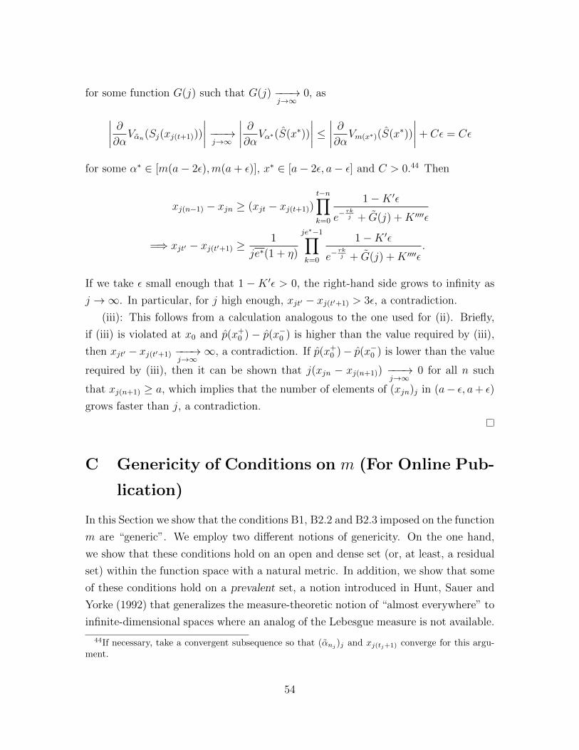
for some function G(j) such that G(j) −−−→j→∞

0, as

∣∣∣∣ ∂∂αVαn(Sj(xj(t+1)))

∣∣∣∣ −−−→j→∞

∣∣∣∣ ∂∂αVα∗(S(x∗))

∣∣∣∣ ≤ ∣∣∣∣ ∂∂αVm(x∗)(S(x∗))

∣∣∣∣+ Cε = Cε

for some α∗ ∈ [m(a− 2ε),m(a+ ε)], x∗ ∈ [a− 2ε, a− ε] and C > 0.44 Then

xj(n−1) − xjn ≥ (xjt − xj(t+1))t−n∏k=0

1−K ′εe−

rkj + G(j) +K ′′′′ε

=⇒ xjt′ − xj(t′+1) ≥1

je∗(1 + η)

je∗−1∏k=0

1−K ′εe−

rkj + G(j) +K ′′′′ε

.

If we take ε small enough that 1 −K ′ε > 0, the right-hand side grows to infinity as

j →∞. In particular, for j high enough, xjt′ − xj(t′+1) > 3ε, a contradiction.

(iii): This follows from a calculation analogous to the one used for (ii). Briefly,

if (iii) is violated at x0 and p(x+0 ) − p(x−0 ) is higher than the value required by (iii),

then xjt′ − xj(t′+1) −−−→j→∞

∞, a contradiction. If p(x+0 )− p(x−0 ) is lower than the value

required by (iii), then it can be shown that j(xjn − xj(n+1)) −−−→j→∞

0 for all n such

that xj(n+1) ≥ a, which implies that the number of elements of (xjn)j in (a− ε, a+ ε)

grows faster than j, a contradiction.

C Genericity of Conditions on m (For Online Pub-

lication)

In this Section we show that the conditions B1, B2.2 and B2.3 imposed on the function

m are “generic”. We employ two different notions of genericity. On the one hand,

we show that these conditions hold on an open and dense set (or, at least, a residual

set) within the function space with a natural metric. In addition, we show that some

of these conditions hold on a prevalent set, a notion introduced in Hunt, Sauer and

Yorke (1992) that generalizes the measure-theoretic notion of “almost everywhere” to

infinite-dimensional spaces where an analog of the Lebesgue measure is not available.

44If necessary, take a convergent subsequence so that (αnj)j and xj(tj+1) converge for this argu-

ment.

54

Claim 1. Consider the set of functions

X1 = {m : [−1, 1] −→ [−1, 1] : m ∈ C1,m weakly increasing }

with the norm ||m|| = max(||m||∞, ||m′||∞). The subset Y1 ⊆ X1 satisfying B1 is

open and dense,45 and also prevalent in the sense of Hunt et al. (1992).

Proof. We first show Y1 is open. Let m0 ∈ Y1; x∗1 < . . . < x∗N be the fixed points of

m0; αi = m′0(x∗i ) for i = 1, . . . , N ; ε > 0 and ν > 0 such that |m′0(y) − 1| ≥ ν for

y ∈ Ii = (x∗i − ε, x∗i + ε) for any i; υ > 0 such that |m(y)− y| ≥ υ for y /∈ Ii for any i;

η = min(ε, υ, ν); and m1 ∈ B(m0, η). Then m1(y) = y implies |m0(y) − y| < η ≤ υ,

so y ∈ Ii for some i, so |m′1(y) − 1| ≥ |m′0(y) − 1| − |m′1(y) − m′0(y)| > ν − ν = 0.

This shows that m′(y) 6= 1 at any fixed point y of m1. Moreover, by construction

either m′0(y) > 1 for all y ∈ Ii and m′1(y) > 1 for all y ∈ Ii as well, or the reverse

inequalities hold, whence m1 can have at most one fixed point in Ii for each i, and

the set of fixed points is finite.

Next, we show Y1 is dense. Let m0 ∈ X1 and ε > 0. We want to show that there

is m1 ∈ B(m0, ε) ∩ Y1. Since m′0 is continuous in [−1, 1], it is uniformly continuous,

so we can take ν > 0 such that if |y − y′| < ν then |m′0(y) −m′0(y′)| < ε4. Partition

[−1, 1] into intervals I1, I2, . . . , IJ as follows: Ij = [yj−1, yj), where yj = −1 + jν, for

j < J , and IJ = [yJ−1, 1]. For each j, if m′0(yj−1) ≥ 1, let m′2(y) = m′0(y) + ε4

for

all y ∈ Ij (which implies m′2(y) > 1 for y ∈ Ij); otherwise let m′2(y) = m′0(y) − ε4

for all y ∈ Ij (so m′2(y) < 1 for y ∈ Ij), and then define m2 by integrating m′2, with

m2(−1) = m0(−1). By construction m2 has at most one fixed point in each interval

Ij and m′2 6= 1 at such points. Moreover, ||m′2 −m′0|| ≤ ε4

and ||m2 −m0|| ≤ 2 ε4

= ε2.

If m2(yj) 6= yj for all yj, we can construct a “smoothed-out” version of m′2, which

we’ll call m′1, that is in B(m0, ε) ∩ Y1. If m2(yj) = yj for some j, and m′2(y) > 1 for

y ∈ Ij ∪ Ij+1 or m′2(y) < 1 for y ∈ Ij ∪ Ij+1, this is not a problem. If m2(yj) = yj

for some j and m′2(y) > 1 for y ∈ Ij, m′2(y) < 1 for y ∈ Ij+1, we can construct a

smooth m′1 such that m′1(yj) = 1, m′1(y) > 1 to the left of yj and < 1 to the right,

and m1(yj) < m2(yj) = yj. The remaining case is analogous.

For the last claim, note that, if a C1 function m defined on a compact interval has

m′ 6= 1 at all its fixed points, it automatically has a finite number of them. Consider

the translation X1−v, where v is the identity function. Then m ∈ Y1 iff m−v has no

45The statement is also true within the space of C3 functions, taken with the appropriate norm.

55

points where (m− v)(y) = (m− v)′(y) = 0. Finally, the fact that Y1 − v is prevalent

in X1 − v follows from Proposition 3 in Hunt et al. (1992).

Claim 2. B2.1 holds in an open set Y2 within

X2 ={m : [x∗, x∗∗] −→ [x∗, x∗∗] : m ∈ C2,m weakly increasing,

m(x∗) = x∗, m(x∗∗) = x∗∗, m(x) < x∀x ∈ (x∗, x∗∗)}

taken with the norm ||m|| = max(||m||∞, ||m′||∞, ||m′′||∞).46

Proof. Trivial.

Claim 3. B2.1’ holds in an open set Y4 within X2.

Proof. This amounts to showing that e is continuous in m′′, and it follows from an

argument similar to the proof of the uniqueness of e from Lemma 6.

Claim 4. Assume u is C3. Let

X3 ={m ∈ Y2 : m ∈ C3, m(x∗) = x∗, m(x∗∗) = x∗∗, m(x) < x∀x ∈ (x∗, x∗∗),

m strictly increasing, m satisfies B2.1}

taken with the norm ||m|| = max(||m||∞, ||m′||∞, ||m′′||∞, ||m′′′||∞). For each y ∈(x∗, x∗∗), the set Y3(y) ⊆ X3 of functions m for which B2.2 and B2.3 hold in [x∗, y]

is open and dense.

Proof. We proceed in two steps. First, we show that the set Y5(y) ⊆ X3 for which

B2.2 holds in [x∗, y] is open and dense. Second, we show that the set Y3(y) is open

and dense within Y5(y).

To show that Y5(y) is open, take m ∈ Y5(y) and suppose there is a sequence (mn)n

such that mn /∈ Y5(y) for all n but mn → m. For each mn we can construct a LS

sn (possibly not unique) by finding a convergent sequence of discrete-time equilibria

(snj)j for δ = e−rj with j → ∞, as in Proposition 8. Using a diagonal argument, we

can find a convergent subsequence of (sn)n, which by continuity must converge to a

LS for m, s. WLOG assume (sn)n → s. We will need the following Lemma:

Lemma 9. If s∗ satisfies Conditions B2.1 and B2.2, then it is the unique LS. More-

over, s∗ has a finite number of vertex points in [x∗, y] for any y < x∗∗.46Again, this is also true within the space of C3 functions.

56

Proof. Briefly, if s∗ has an infinite number of vertex points in [x∗, y], they must

accummulate at some y∗ ∈ (x∗, y], which must satisfy Vm(y∗)(S(y∗)) =∂Vm(y∗)(S(y∗))

∂α=

0. If∂2Vm(y∗)(S(y∗))

∂α2 > 0 we obtain V > 0 in a neighborhood of y∗, a contradiction.

If∂2Vm(y∗)(S(y∗))

∂α2 < 0 this guarantees Condition B2.3 in a neighborhood of y∗, which

means the vertex points near y∗ must be part of a single sequence, contradicting

Lemma 7.

Suppose that there are infinitely many vertex points on a left-neighborhood of

y∗ (the other case is analogous). Similar arguments apply if∂3Vm(y∗)(S(y∗))

∂α3 < 0 or∂3Vm(y∗)(S(y∗))

∂α3 > 0, respectively.

As for the uniqueness of s∗, the proof in Lemma 8 can be extended to this case.

From this we conclude that s = s∗. Letting Wn be the value function for sn,

we then have Wn → W . It can be shown in addition that, at every y that is not a

vertex point of s∗, W′n(y)→ W ′(y), W ′′

n (y)→ W ′′(y) and W ′′′n (y)→ W ′′′(y), by using

Lemmas 6 and 9.

Next, we show that Y5(y) is dense. Take m ∈ X3 and ε > 0. Consider m given by:ˆm(x∗) = x∗, m′(x∗) = m′(x∗), m′′(x∗) = m′′(x∗) and m′′′(x) = m′′′(x) + η(x), where

|η(x)| ≤ ε will be defined as 0 except where we specify otherwise. We will argue that,

by picking η correctly, we can find a m ∈ Y5(y) that is close to m.

Apply the following algorithm. Take ν > 0 small and N > 0 large. Let η0 ≡ 0

and m0 ≡ m. Let

x0 = inf

{x ∈ (x∗, y] : max

(∣∣Vm0(x)(S0(x))∣∣ , ∣∣∣∣ ∂∂αVm0(x)(S0(x))

∣∣∣∣ ,∣∣∣∣ ∂2

∂α2Vm0(x)(S0(x))

∣∣∣∣ , ∣∣∣∣ ∂3

∂α3Vm0(x)(S0(x))

∣∣∣∣) ≤ ε

N

},

where S0(x) is a the policy path starting at x for a LS given median voter function

m0.47 Let α0 = m(x0). Define η1(x) = −ε for x ∈ [x0, x′0) and η1(x) = 0 for all

other x, with x′0 taken so that m1(x′0) = m1(x0) + ν. Next, let x1 be the infimum

of x ∈ (x0 + ν, y] for which |Vm1(x)(S1(x))|, | ∂∂αVm1(x)(S1(x))|, | ∂2

∂α2Vm1(x)(S1(x))| and

| ∂3∂α3Vm1(x)(S1(x))| ≤ ε

N, and define α1 = m(x1) and η2(x) = −ε for x ∈ [x1, x

′1) and

η2(x) = η1(x) for all other x, with x′1 taken so that m2(x′1) = m2(x1) + ν. Define xk,

47Note that, for ε small enough, x0 > x∗ since e(x) ≥ C > 0 in a neighborhood of x∗, which

implies ∂2

∂α2Vm0(x)(S0(x)) ≥ C ′ > 0.

57

αk, ηk+1, mk+1 for k = 2, 3, . . . in the same fashion until xK = +∞ for some K.48 Let

m = mK .

We argue that, if ν and N are taken to be small and large enough, respectively,

m satisfies Condition B2.2. To explain why, we will need the following

Remark 5. A function f : [a, b]→ R is uniformly continuous iff there is an increasing

function h : [0,+∞) → [0,+∞) such that h(0) = 0, h is continuous at 0, and

|f(x) − f(y)| ≤ h(|x − y|) for all x, y ∈ [a, b]. We say a function h satisfying these

properties is a bounding function.

Now note that, for any k and any x < x′ such that m(x) = a, m(x′) = a′ satisfy

a, a′ ∈ [αk, αk + ν], we have∣∣∣∣ ∂3

∂α3Va(S(x))− ∂3

∂α3Va′(S(x′))

∣∣∣∣ ≤ ∣∣∣∣ ∂3

∂α3Ua(S(x))− ∂3

∂α3Ua(S(x′))

∣∣∣∣+

∣∣∣∣ ∂3

∂α3Ua(S(x′))− ∂3

∂α3Ua′(S(x′))

∣∣∣∣+

∣∣∣∣− d3

dα3ua(m

−1(a)) +d3

dα3ua′(m

−1(a′))

∣∣∣∣≤∣∣∣∣ ∂3

∂α3Ua(S(x))− ∂3

∂α3Ua(S(x′))

∣∣∣∣+ h1(a′ − a) + h2(a′ − a)

≤K ε

N+K ′(a′ − a) + h1(a′ − a) + h2(a′ − a) ≤ K

ε

N+ h3(a′ − a)

where h1, h2, h3 are bounding functions, K,K ′ > 0, and K, h1, h2, h3 are independent

of ν and N .

The bound | d3dα3ua(m

−1(a)) + d3

dα3ua′(m−1(a′))| ≤ h2(|a − a′|) uses the uniform

continuity of d3

dα3ua(m−1(a)), which follows from the fact that u is C3 and m is C3

on [a, a′] ⊆ [αk, αk + ν]. The bound | ∂3∂α3Ua(S(x′)) − ∂3

∂α3Ua′(S(x′))| ≤ h1(|a − a′|)uses the uniform continuity of ∂3

∂α3U , and the fact that the mapping x 7→ max(x, 0) is

Lipschitz. The first bound is the trickiest, and is based on the idea that, if ∂V∂α

and∂2V∂α2 are low, then s(x, t) changes relatively quickly as a function of t, so S(x) and

48This must happen for a finite K, as αk − αk−1 ≥ ν > 0 for all k.

58

S(x′) are similar. Formally:∣∣∣∣ ∂3

∂α3Ua(S(x))− ∂3

∂α3Ua(S(x′))

∣∣∣∣ ≤ (1− e−rd(x′,x))

2 maxa,y

∂3

∂α3uα(y)

1− e−rd(x′,x) ≤ rd(x′, x) = r

∑yl∈(x,x′)

vertex point

el +

� x′

x

e(y)dy

≤ r2

r

∑yl∈(x,x′)v.p.

(erel2 − 1) + re(x′ − x) ≤

≤ 2∑

yl∈(x,x′)v.p.

|max m′|minx∈[x0,y]

∣∣∣∂um(x)(x)

∂x

∣∣∣∣∣∣∣ ∂∂αVal(S(y−l ))

∣∣∣∣+ re(x′ − x) ≤

≤ K ′′

(∣∣∣∣ ∂∂αVa(S(x))

∣∣∣∣+

� a′

a

∣∣∣∣ ∂2

∂α2Va(S(n(a)))

∣∣∣∣ da)

+ re(x′ − x) ≤ K ′′ε

N+K ′′′(a′ − a).

Pick ν and N so that K εN

+ h3(ν) ≤ ε2

and N ≥ 4. Now m satisfies Condition B2.2

because, for a ∈ [αk, αk + ν),∣∣∣∣ ∂3

∂α3Va(S(x))

∣∣∣∣ ≥ ∣∣∣∣ ∂3

∂α3Vαk(S(xk))

∣∣∣∣−∣∣∣∣ ∂3

∂α3Vαk(S(xk))−

∂3

∂α3Va(S(x))

∣∣∣∣ ≥ ε− ε

N− ε

2≥ ε

4> 0.

On the other hand, if a /∈ [αk, αk+ν) for any k, then | ∂i∂αiV | > ε

Nfor some i = 0, 1, 2, 3

by construction.

The only remaining issue is that m is not C3 because ηK is not continuous at αk

and αk + ν for k = 0, 1, . . . , K − 1. However, it is easy to construct a continuous η

close to ηK that fixes this problem.49

Next, we argue that Y3(y) is open. As shown in Proposition 8, Conditions B2.1,

B2.2 and B2.3 taken together imply that the equilibrium path s(x, t) will be given

by either a smooth path with e(x) > 0 for all x ∈ (x∗, y] or a smooth path up to

some y0 followed by a finite sequence of jumps and stops with stops at y1, y2, . . . , yl.

It is enough to show that e′ is continuous in m′′′, which follows from the arguments in

Proposition 8, and that yi is continuous in m′′′ for i = 1, 2, . . . , l, which is elementary

(in fact, yi is continuous in m′).

Finally we argue that Y3(y) is dense. Take m ∈ X3 and ε > 0. Because Y5(y)

49WLOG, take a = αk. If Va(S(x−)) > 0, it is easy to perturb ηK to make it continuous at awithout violating Condition B2.2. If not, but Va(S(x−)) > 0 for a < a arbitrarily close to a, we can

perturb ηK at one such a instead. If Va(S(x−)) = 0 for all a < a close to a, but ∂2

∂α2V is nonzero

close to a, we can do the same argument. If ∂2

∂α2V is also zero in an interval to the left of a, thenCondition B2.2 would be violated for a < a, a contradiction.

59

is dense, there is m ∈ B(m, ε) ∩ Y5(y). Because Y5(y) is open, there is ε′ > 0 such

that B(m, ε′) ⊆ B(m, ε) ∩ Y5(y). Next, we claim that there is ˆm ∈ B(m, ε′) ∩ Y3(y),

which completes the proof. This can be shown by construction. If e(x) > 0 for all

x ∈ [x∗, y], we are done. If not, s induces a policy path that is continuous up to some

y0 and then features a sequence of jumps and stops with stops at y1, y2, . . . , yl. (By

the arguments in Proposition 8, this sequence cannot be infinite.) If Condition B2.3

holds at y1, . . . , yl, we are done. If not, suppose WLOG that it first fails at yl. m

can be perturbed near yl to obtain m2 ∈ B(m, ε′) that satisfies Condition B2.3 at

y1, . . . , yl. Similarly, if m2 first fails Condition B2.3 at some yl′ > yl, we can construct

m3 ∈ B(m, ε′), a perturbation of m2 near yl′ , that satisfies Condition B2.3 up to

yl′ . If this process stops in a finite number of steps, we are done. If not, let m∞ be

the pointwise limit of (mk)k. m∞ must feature an infinite sequence of vertex points

y1 < y2 < . . . with yl −−−−→l→+∞

y∗ ≤ y, but, as m∞ ∈ Y5(y), m∞ satisfies Condition

B2.2, leading to a contradiction.

Corollary 3. The set Y3 ⊆ X3 of functions for which B2.2 and B2.3 hold in [x∗, x∗∗]

is a residual set.

Claim 5. In the case of quadratic utility, the set of functions m for which B2.2 holds

for x ∈ (x∗, x∗ + d) is prevalent.

Proof. The result follows from Theorem 3 in Hunt et al. (1992). Following their

notation, take M = {y ∈ R4 : 2y3−1y1−y2 + y4

y3= 0} and Z = {y ∈ R5 : (y1, y2, y3, y4) ∈

M and 2y4(y1−y2)−2y3(1−y3)(y1−y2)2

+y5y3−y24

y23= 0}. We need to check that M is a manifold

of codimension 1, and that the projection π : M −→ R given by y 7−→ y1 is a

submersion; both follow from the Implicit Function Theorem. Finally, we need to

check that Z is a zero set in M × R, which can also be shown using the Implicit

Function Theorem. Theorem 3 from Hunt et al. (1992) then implies that the set of

functions m for which there is an x such that

e(x) =2m′(x)− 1

x−m(x)+m′′(x)

m′(x)= 0 =

=2m′′(x)(x−m(x))− 2m′(x)(1−m′(x))

(x−m(x))2+m′′′(x)m′(x)−m′′(x)2

m′(x)2= e′(x)

is shy, i.e., its complement is prevalent.

60

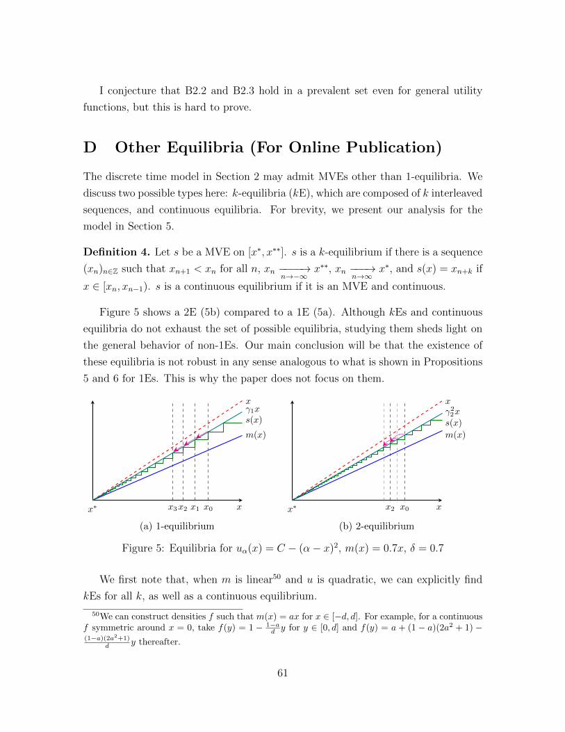
I conjecture that B2.2 and B2.3 hold in a prevalent set even for general utility

functions, but this is hard to prove.

D Other Equilibria (For Online Publication)

The discrete time model in Section 2 may admit MVEs other than 1-equilibria. We

discuss two possible types here: k-equilibria (kE), which are composed of k interleaved

sequences, and continuous equilibria. For brevity, we present our analysis for the

model in Section 5.

Definition 4. Let s be a MVE on [x∗, x∗∗]. s is a k-equilibrium if there is a sequence

(xn)n∈Z such that xn+1 < xn for all n, xn −−−−→n→−∞

x∗∗, xn −−−→n→∞

x∗, and s(x) = xn+k if

x ∈ [xn, xn−1). s is a continuous equilibrium if it is an MVE and continuous.

Figure 5 shows a 2E (5b) compared to a 1E (5a). Although kEs and continuous

equilibria do not exhaust the set of possible equilibria, studying them sheds light on

the general behavior of non-1Es. Our main conclusion will be that the existence of

these equilibria is not robust in any sense analogous to what is shown in Propositions

5 and 6 for 1Es. This is why the paper does not focus on them.

x∗ x3x2 x1 x0

xγ1xs(x)

m(x)

x

(a) 1-equilibrium

x∗ x2 x0

xγ22xs(x)

m(x)

x

(b) 2-equilibrium

Figure 5: Equilibria for uα(x) = C − (α− x)2, m(x) = 0.7x, δ = 0.7

We first note that, when m is linear50 and u is quadratic, we can explicitly find

kEs for all k, as well as a continuous equilibrium.

50We can construct densities f such that m(x) = ax for x ∈ [−d, d]. For example, for a continuousf symmetric around x = 0, take f(y) = 1 − 1−a

d y for y ∈ [0, d] and f(y) = a + (1 − a)(2a2 + 1) −(1−a)(2a2+1)

d y thereafter.

61

Proposition 9. Let uα(x) = C − (α − x)2 and m(x) = ax for x ∈ [−d, d]. Assume

δ ≥ 23

and a ∈(

12, 1). Then, for each k and x < d, there is a kE sk restricted to [−d, d]

such that x0 = x, given by xn = γnkx, where γk ∈ (0, 1). There is also a continuous

equilibrium s∞ given by s∞(x) = γ∞x. γkk is decreasing in k and γkk → γ∞.

Proof of Proposition 9. Given k ≥ 1, assume a kE of the form s(xn) = γkkxn. Since

s(xn) = xn+k but s(xn − ε) = xn+k+1, m(xn) must be indifferent between xn+k and

xn+k+1. This implies

−∑

δt(axn − xn+(t+1)k)2 = −

∑δt(axn − xn+(t+1)k+1)2∑

δt(a− γ(t+1)k)2 =∑

δt(a− γ(t+1)k+1)2

γk(1 + γ)

1− δγ2k=

2a

1− δγk

We now argue that the expression γk−δγ2k1−δγ2k is increasing in γ. It is equivalent to show

that x−δx21−δx2 is increasing in x for x ∈ [0, 1]. This is true because x− δx2 ≤ 1− δx2 but

1− 2δx > −2δx, so the log-derivative of x−δx21−δx2 is positive. Hence, (γk−δγ2k)(1+γ)

1−δγ2k is also

increasing in γ, and equals 2a for a unique value of γ which we denote γk ∈ (0, 1).

Denote Ak(x) = (x−δx2)(1+x1k )

1−δx2 . Then Ak(γkk) = 2a for all k, and Ak(x) is increasing

in x and k. It follows that γkk is decreasing in k.

We now show that the constructed sk supports an MVE. By the same argu-

ment given in Proposition 5 for 1Es, since m(xn) is indifferent between S(xn+k) and

S(xn+k+1), all α > m(xn) strictly prefer S(xn+k) to S(xn+k+1), and α < m(xn) strictly

prefer S(xn+k+1). Hence, m(xn) prefers S(xn+k) to S(xr) for all r 6= n+ k.

Next, we show that m(xn) prefers xn+k to other policies x /∈ (xn)n. We do this in

two steps. First, we argue that γk+1 > a, which implies xn+k+1 > m(xn). Second, we

note that this yields our result by the same argument as in Proposition 5. For the

first part, note that γk+1 > a iff

(γk + γk+1)(1− δγk) < 2γk+1(1− δγ2k)

⇐⇒ (1− γ) < δ(γk(1− γk+1) + γk+1(1− γk)

)⇐⇒ 1 < δ

(γk + 2γk+1 + . . .+ 2γ2k

)Note that Ak is decreasing in δ, so γ is increasing in δ and a. Hence the worst case

is δ = 23, a = 1

2. Now suppose k = 1. Then the required inequality is 1 < 2

3(γ + 2γ2),

62

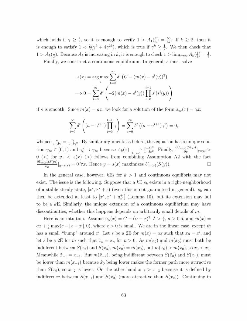
which holds if γ ≥ 23, so it is enough to verify 1 > A1(2

3) = 50

57. If k ≥ 2, then it

is enough to satisfy 1 < 23(γk + 4γ2k), which is true if γk ≥ 1

2. We then check that

1 > Ak(12). Because Ak is increasing in k, it is enough to check 1 > limk→∞Ak(

12) = 4

5.

Finally, we construct a continuous equilibrium. In general, s must solve

s(x) = arg maxy

∞∑t=0

δt(C − (m(x)− st(y))2

)=⇒ 0 =

∞∑t=0

δt

(−2(m(x)− st(y))

t−1∏i=0

s′(si(y))

)

if s is smooth. Since m(x) = ax, we look for a solution of the form s∞(x) = γx:

∞∑t=0

δt

((a− γt+1)

t−1∏i=0

γ

)=∞∑t=0

δt((a− γt+1)γt

)= 0,

whence a1−δγ = γ

1−δγ2 . By similar arguments as before, this equation has a unique solu-

tion γ∞ ∈ (0, 1) and γkk → γ∞ because Ak(x) −−−→k→∞

x−δx21−δx2 . Finally,

∂Um(x)(S(y))

∂y|y=y0 >

0 (<) for y0 < s(x) (>) follows from combining Assumption A2 with the fact∂Um(x)(S(y))

∂y|y=s(x) = 0 ∀x. Hence y = s(x) maximizes Um(x)(S(y)).

In the general case, however, kEs for k > 1 and continuous equilibria may not

exist. The issue is the following. Suppose that a kE sk exists in a right-neighborhood

of a stable steady state, [x∗, x∗ + ε) (even this is not guaranteed in general). sk can

then be extended at least to [x∗, x∗ + d+x∗ ] (Lemma 10), but its extension may fail

to be a kE. Similarly, the unique extension of a continuous equilibrium may have

discontinuities; whether this happens depends on arbitrarily small details of m.

Here is an intuition. Assume uα(x) = C − (α − x)2, δ > 23, a > 0.5, and m(x) =

ax+ a4

max(c− |x− x′|, 0), where c > 0 is small. We are in the linear case, except m

has a small “bump” around x′. Let s be a 2E for m(x) = ax such that x0 = x′, and

let s be a 2E for m such that xn = xn for n > 0. As m(x0) and m(x0) must both be

indifferent between S(x2) and S(x3), m(x0) = m(x0), but m(x0) > m(x0), so x0 < x0.

Meanwhile x−1 = x−1. But m(x−2), being indifferent between S(x0) and S(x1), must

be lower than m(x−2) because x0 being lower makes the former path more attractive

than S(x0), so x−2 is lower. On the other hand x−3 > x−3 because it is defined by

indifference between S(x−1) and S(x0) (more attractive than S(x0)). Continuing in

63

this fashion, the subsequence (x0, x−2, x−4, . . .) is lower than (x0, x−2, . . .), and the

opposite is true for the odd elements. Eventually x2l < x2l+1 for some l, i.e., the even

subsequence becomes so attractive that a voter m(x2l+1), though indifferent between

S(x2l+3) and S(x2l+4), instead prefers S(x2l+2) to both, so no one votes for x2l+3.

kEs for k > 1 are unstable for this reason. We now give a local argument to this

effect. Let En = (1− δ)∑∞t=0 δtxn+tk, Wn = (1− δ)∑∞t=0 δ

tx2n+tk, and characterize a

kE recursively as follows, using the indifference of m(xn) between Sn+k and Sn+k+1,

i.e., −(m(xn)− En+k)2 −Wn+k = −(m(xn)− En+k+1)2 −Wn+k+1:

En = (1− δ)xn + δEn+k = (1− δ)m−1

(1

2

Wn+k −Wn+k+1

En+k − En+k+1

)+ δEn+k

Wn = (1− δ)x2n + δWn+k = (En − δEn+k)xn + δWn+k

Taking Yn = (En, . . . , En+k+1,Wn+1, . . . ,Wn+k+1) as the state variable of the recur-

sion, its linearization around an equilibrium is given by Yn = MnYn+1, where

Mn =

0 . . . 0 A B 0 . . . 0 C D

1 0 · · · 0

0 1 · · · 0...

.... . .

...

0 0 · · · 1

0

0...

0

0 0 · · · 0 0

0 0 · · · 0 0...

.... . .

......

0 0 · · · 0 0

2x 0 . . . 0 −2δx 0 0 . . . 0 δ

0 0 · · · 0

0 0 · · · 0...

.... . .

...

0 0 · · · 0

0

0...

0

1 0 · · · 0 0

0 1 · · · 0 0...

.... . .

......

0 0 · · · 1 0

}1 k

}1 k − 1

where x = xn+1; B = ∂En∂En+k+1

, D = ∂En∂Wn+k+1

and so on. Note that

det(Mn) = −δB − 2δxn+1D = δ(1− δ) xn+1 −m(xn)

m′(xn)(En+k − En+k+1)

64

det(Mn . . .Mn−k+1) ≥ δk(1− δ)k[

min0≤l≤k−1

(xn−l+1 −m(xn−l)

m′(xn−l)

)]k1∏k−1

l=0 (En−l+k − En−l+k+1)

≥ δk(1− δ)k[

min0≤l≤k−1

(xn−l+1 −m(xn−l)

m′(xn−l)

)]kkk

(En+1 − En+k+1)k

= δk[

min0≤l≤k−1

(xn−l+1 −m(xn−l)

m′(xn−l)

)]kkk

(xn+1 − En+k+1)k

where we have used the AM-GM inequality. Now, if δ is close to 1 and the equilibrium

is close to a CLS in the sense of Proposition 6, then x−m(x)m′(x)(x−E(S(s(x))))

≈ 1 (see Ap-

pendix B) and det(Mn . . .Mn−k+1) ≈ kk. (In particular, these statements hold with

equality for the linear case we have solved above.) Hence there must be an eigenvalue

of absolute value at least kk

2k+1 > 1. Thus any deviation from an equilibrium result-

ing from a local perturbation of m which adds a nonzero component to a generalized

eigenvector of this eigenvalue (in the Jordan form decomposition of the matrix) will

grow exponentially.

Similarly, in the example given above of a linear m with a bump, a continuous

equilibrium constructed up to x′ − c would have a discontinuity at s−1(x′). This

insight extends more generally. For brevity, we show this for smooth (C∞) equilibria.

Proposition 10. Assume ua(x) = C − (α − x)2. Let s : [x∗, x∗∗) → [x∗, x∗∗) be

a smooth equilibrium for a given m. Let x0 ∈ (x∗, x∗∗). A perturbation m of m

is an increasing function m = m + ρκ where κ : [x∗, x∗∗) → [x∗, x∗∗) has support

(x0 − ε, x0 + ε). For each m, let s be an equilibrium under m such that s|[x∗,x0−ε) =

s|[x∗,x0−ε).Suppose m is C∞. Then, if κ is Ck but its (k+ 1)th derivative has a discontinuity

in (x0 − ε, x0 + ε), s has a discontinuity in [x∗, s−k−1(x0 + ε)] for all ρ 6= 0.

Proof. Denote E(y) = E(S(y)), W (y) = W (S(y)), and 12∂W (y)∂E(y)

= L−1(y). Then

s(x) = arg maxy

−m(x)2 + 2m(x)E(y)−W (y)⇒ m(x) =1

2

∂W (y)

∂E(y)|s(x)

s(x) =

(1

2

∂W (y)

∂E(y)

)−1

(m(x)) = L(m(x))

(W,E)(x) =((1− δ)x2 + δW (L(m(x))), (1− δ)x+ δE(L(m(x)))

)In particular, W (E) must be a strictly convex function so that s is surjective, and it

must have no kinks, i.e., s must be strictly increasing (if s is locally constant at x,

65

it will be discontinuous at s−1(x) as long as s(y) > m(y) in this area), so L−1 and L

are strictly increasing and well-defined.

Now suppose E is C l+1 around s(s(x)) but s has a (l + 1)-kink at s(x), i.e., it is

C l+1 in (s(x)− η, s(x))∪ (s(x), s(x) + η) but only C l in (s(x)− η, s(x) + η). Then s′

has a l-kink at s(x). Since

∂W (y)

∂E(y)=

∂W (y)∂y

∂E(y)∂y

=2(1− δ)y + δW ′(s(y))s′(y)

(1− δ) + δE ′(s(y))s′(y)

=W ′(s(y))

E ′(s(y))+

(1− δ)(2y − W ′(s(y))E′(s(y))

)

1− δ + δE ′(s(y))s′(y)= 2m(y) +

(1− δ)(2y − 2m(y))

1− δ + δE ′(s(y))s′(y),

L−1 has a l-kink at s(x); L has a l-kink at m(x); and s has a l-kink at x.

Then, if κ has a (k+1)-kink at x, then m has a (k+1)-kink at x; s has a (k+1)-kink

at x; s has a k-kink at s−1(x); . . . and s has a discontinuity at s−k−1(x).

A similar result holds even for smooth perturbations.

Proposition 11. Assume ua(x) = C − (α − x)2. Let s : [x∗, x∗∗) → [x∗, x∗∗) be a

smooth equilibrium for a given m with m′ ≥ A > 12

everywhere. Let z ∈ (x∗, x∗∗) and

z′ = s(z). Given a smooth function κ : [x∗, x∗∗)→ [x∗, x∗∗) with support contained in

[z′, z] and ρ ∈ R, let mρ = m+ρκ, and let sρ be the unique equilibrium under mρ that

equals s within [x∗, z′], if it exists. Then there exists κ such that sρ is discontinuous

for all ρ 6= 0.

Proof. Pick K ∈ N and define a set of 2K sequences (yni) (n ∈ Z, i ∈ {1, . . . , 2K})as follows. y01 = z′, y0(2K) = z, (y0i)i is an arithmetic sequence, and, for all n, i,

y(n+1)i = s(yni).

Let κ be a non-negative C∞ function with support [0, 1] such that κ(12) = 1.

Define κ(x) =∑

i≤2K odd κ(

x−y0iy0(i+1)−y0i

), so that κ has a copy of κ “squeezed” into

each interval [y0i, y0(i+1)] for i odd. Any such κ will work.

We write W (E) to denote W (E−1(E)), Wρ to denote W with perturbation ρκ, etc.

Assume ρ > 0. It is easy to show that sρ(x) ≡ s(x) for x ∈ [yni, yn(i+1)] for all n and

even i, and sρ(x) > s(x) for x ∈ [y0i, y0(i+1)] for odd i (because sρ(x) = s(y) whenever

mρ(x) = m(y)). In addition, and Wρ(E) < W (E) for x ∈ [E(y0i), E(y0(i+1))] for odd

i, since ∂W∂E

(y) = 2m(y) but, for a path (xt)t, decreasing x0 by ε decreases E((xt)t) by

(1− δ)ε and W ((xt)t)) by (1− δ)ε(2x0 − ε), that is, ∆W∆E≈ 2x0 > 2m(x0).

66

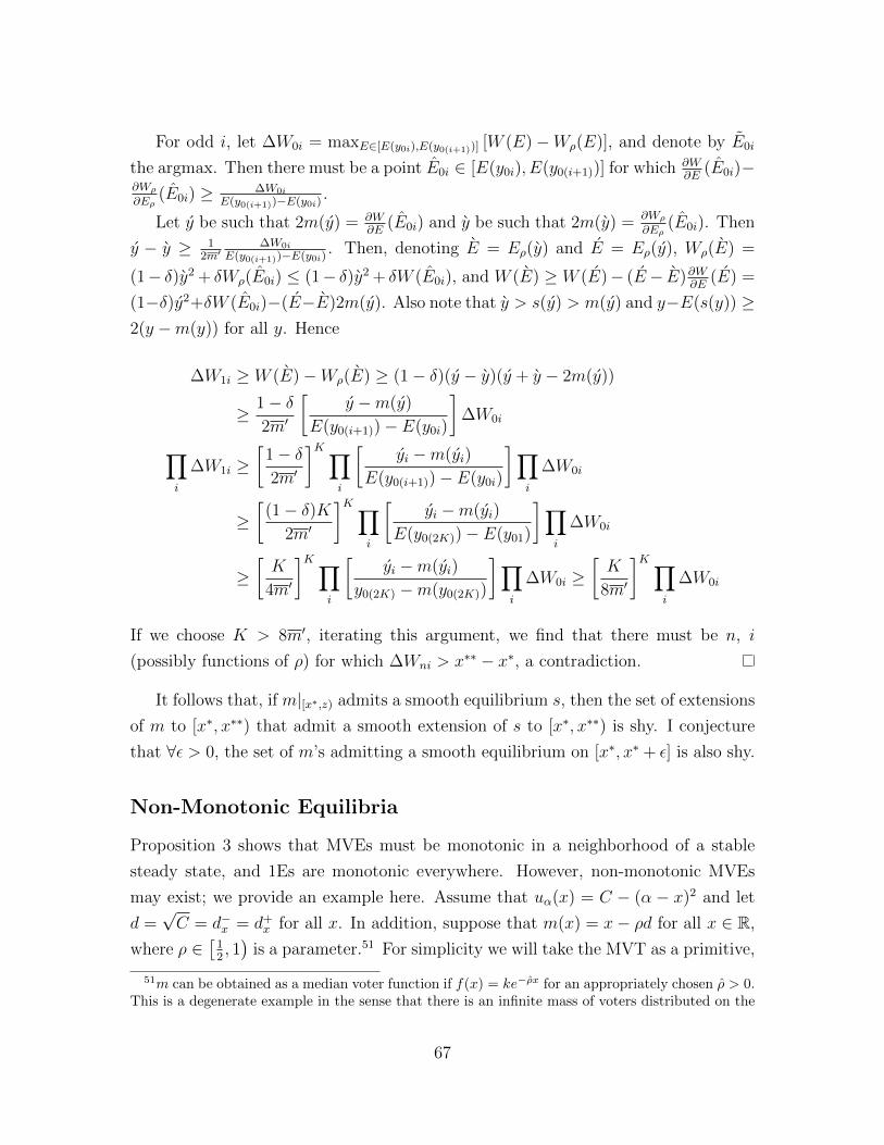
For odd i, let ∆W0i = maxE∈[E(y0i),E(y0(i+1))] [W (E)−Wρ(E)], and denote by E0i

the argmax. Then there must be a point E0i ∈ [E(y0i), E(y0(i+1))] for which ∂W∂E

(E0i)−∂Wρ

∂Eρ(E0i) ≥ ∆W0i

E(y0(i+1))−E(y0i).

Let y be such that 2m(y) = ∂W∂E

(E0i) and y be such that 2m(y) = ∂Wρ

∂Eρ(E0i). Then

y − y ≥ 12m′

∆W0i

E(y0(i+1))−E(y0i). Then, denoting E = Eρ(y) and E = Eρ(y), Wρ(E) =

(1− δ)y2 + δWρ(E0i) ≤ (1− δ)y2 + δW (E0i), and W (E) ≥ W (E)− (E− E)∂W∂E

(E) =

(1−δ)y2+δW (E0i)−(E−E)2m(y). Also note that y > s(y) > m(y) and y−E(s(y)) ≥2(y −m(y)) for all y. Hence

∆W1i ≥ W (E)−Wρ(E) ≥ (1− δ)(y − y)(y + y − 2m(y))

≥ 1− δ2m′

[y −m(y)

E(y0(i+1))− E(y0i)

]∆W0i

∏i

∆W1i ≥[

1− δ2m′

]K∏i

[yi −m(yi)

E(y0(i+1))− E(y0i)

]∏i

∆W0i

≥[

(1− δ)K2m′

]K∏i

[yi −m(yi)

E(y0(2K))− E(y01)

]∏i

∆W0i

≥[K

4m′

]K∏i

[yi −m(yi)

y0(2K) −m(y0(2K))

]∏i

∆W0i ≥[K

8m′

]K∏i

∆W0i

If we choose K > 8m′, iterating this argument, we find that there must be n, i

(possibly functions of ρ) for which ∆Wni > x∗∗ − x∗, a contradiction.

It follows that, if m|[x∗,z) admits a smooth equilibrium s, then the set of extensions

of m to [x∗, x∗∗) that admit a smooth extension of s to [x∗, x∗∗) is shy. I conjecture

that ∀ε > 0, the set of m’s admitting a smooth equilibrium on [x∗, x∗ + ε] is also shy.

Non-Monotonic Equilibria

Proposition 3 shows that MVEs must be monotonic in a neighborhood of a stable

steady state, and 1Es are monotonic everywhere. However, non-monotonic MVEs

may exist; we provide an example here. Assume that uα(x) = C − (α − x)2 and let

d =√C = d−x = d+

x for all x. In addition, suppose that m(x) = x− ρd for all x ∈ R,

where ρ ∈[

12, 1)

is a parameter.51 For simplicity we will take the MVT as a primitive,

51m can be obtained as a median voter function if f(x) = ke−ρx for an appropriately chosen ρ > 0.This is a degenerate example in the sense that there is an infinite mass of voters distributed on the

67

i.e., we will analyze the game in which m(x) picks s(x).

Assume δ = 0. Then s(x) = m(x), so S(s(x)) = (x − ρd, x − 2ρd, x − 3ρd, . . .).

Crucially x− ρd, x− 2ρd ∈ (m(x)− d,m(x) + d) but x− 3ρd /∈ (m(x)− d,m(x) + d).

Now, suppose that δ is small but positive. Assume a successor function s1 of the

form s1(x) = x−ρd+η1 with η1 small, such that s21(x) > m(x)−d but s3

1(x) < m(x)−d.

For s1 to be an equilibrium, η1 must maximize

um(x)(x− ρd+ η) + δum(x)(s1(x− ρd+ η)) = C(1 + δ)− η2 − δ(ρd− η1 − η)2

=⇒ η1 =δ

1 + 2δρd.

Note that, since η1 > 0, this calculation will be invalid for ρ close enough to 12, as in

fact we will then have s31(x) > m(x)− d.

Next, assume a successor function s2(x) = x− ρd+ η2 with η2 such that s32(x) >

m(x)− d but s42(x) < m(x)− d. For s2 to be an equilibrium, we must have

η2 = arg maxη′

um(x)(x− ρd+ η′) + δum(x)(s2(x− ρd+ η′)) + δ2um(x)(s22(x− ρd+ η′))

=⇒ η2 =δ + 2δ2

1 + 2δ + 3δ2ρd.

Now suppose that s2 is being played, and x considers deviating to some η3 such

that s22(x− ρd+ η3) < m(x)− d. The (locally) optimal η3 must satisfy

−2η3 − 2δ(η3 + η2 − ρd) = 0 =⇒ η3 =δ

1 + δ(ρd− η2) =

δ

1 + δ

1 + δ + δ2

1 + 2δ + 3δ2ρd.

Note that η2 > η1 > η3 > 0. In particular, since η2 > η3, we can choose ρ, δ

so that x − 3ρd + 3η2 > m(x) − d > x − 3ρd + η3 + 2η2. Furthermore, we can

choose them so that Um(x)(S2(x− ρd+ η3)) = Um(x)(S2(x− ρd+ η2)).52 If we choose

our parameters this way then m(x) is indifferent about deviating (this is true for all

x). Now construct a successor function s as follows: s(x) = s2(x) for all x < x0;

s(x0) = x− ρd+ η3; and s(x) for x > x0 is defined by backward induction. This is a

non-monotonic equilibrium by construction. While this example relies on indifference,

real line, as opposed to a unit mass with support [−1, 1], but it allows for a simpler construction.52This follows from a continuity argument: when s22(x− ρd+ η3) = m(x)− d, Um(x)(S2(x− ρd+

η3)) < Um(x)(S2(x−ρd+η2)), whereas when s22(x−ρd+η2) = m(x)−d then Um(x)(S2(x−ρd+η3)) >Um(x)(S2(x−ρd+η2)), so we can choose intermediate values of ρ, δ for which Um(x)(S2(x−ρd+η3)) =Um(x)(S2(x− ρd+ η2)).

68

we can adjust m to make it strict.

E Additional Results (For Online Publication)

E.1 Supermajority Requirements and Other Decision Rules

We assume as part of our solution concept that chosen policies are Condorcet winners.

The analysis readily extends to other decision rules. We briefly discuss two.

First, suppose that, given a policy x and a set of members I(x), an unmodeled

political process gives some agent n(x) the right to choose tomorrow’s policy. (For

example, the function n(x) might reflect the notion that the policy x affects the

relative power of different agents within the organization.) All the results extend to

this case, substituting n(x) for m(x), even if n(x) is not a median voter function.

Second, consider an organization with a bias towards inaction in which policy

changes require a supermajority ρ > 12. Define mp(x) as the pth percentile-member

of I(x), and assume that a policy y > x can only be chosen over the current policy

x if m1−ρ(x) votes for it, while a change to y < x is only possible if mρ votes for

it. It follows that, in intervals where x > mρ(x), the game is equivalent to the main

model with n(x) = mρ(x); in intervals where x < m1−ρ(x), it is equivalent to setting

n(x) = m1−ρ(x); and in intervals where m1−ρ(x) < x < mρ(x), no policy changes are

possible. In other words, steady states are now intervals rather than points, and we

will observe lower policy drift, but the gist of the results is unchanged.

E.2 Positive Entry and Exit Costs

The main model assumes free entry and exit. This assumption adds a lot of tractabil-

ity, but is rarely exactly true in a descriptive sense. Here, we demonstrate that our

results are also relevant in a setting with positive entry and exit costs. We begin

by considering a variant of the game with only entry costs: every time an outsider

chooses to join the club, she must pay a cost c > 0.

A full extension of the results to this case is difficult because the introduction of

entry costs adds intertemporal concerns to entry and exit decisions: agents considering

entry now need to think about what the policy will be several periods from now,

whether they will want to leave later, etc. Relatedly, agents with identical preferences

may behave differently depending on their current status: if the policy x is stable over

69

time, and an agent α’s flow payoff from membership, uα(x), is positive but very small,

then α would choose to remain in the club if she is already a member but not bother

entering otherwise. As a result, the club’s current policy is no longer the only payoff-

relevant state variable; It is now an (infinite-dimensional) state variable as well.

In spite of this, the main thrust of the paper’s results—namely, that the club

should converge to a myopically stable policy—still carries over in this model if we

impose some reasonable simplifications. Concretely, we will assume the following:

(i) As in Section 4, we restrict the analysis to [x∗, x∗∗], the right side of the basin

of attraction of a stable steady state x∗.

(ii) Assume xt+1 ≤ xt for all x ∈ [x∗, x∗∗], i.e., the policy cannot move to the right.

(iii) Assume an initial x0 ∈ [x∗, x∗∗] such that ux0−dx0 (x∗) ≥ (1−δ)c. In other words,

x0 is close enough to x∗ that all agents who might consider joining the club as

the policy moves left from x0 will strictly prefer not to quit later.53

(iv) Assume an initial set of members I0 = I(x0).

(v) Voting behavior at time t can condition on It only up to a set of measure zero,

i.e., if I1, I2 differ by a set of Lebesgue measure zero then s(I1) = s(I2).

An MVE of this game is given by mappings s(I) and I(x, I ′) satisfying the above

conditions such that I reflects optimal entry and exit decisions given current policy

x, an existing set of members I ′ and the expected continuation; and S(s(I)) is a

Condorcet winner among all S(y) for the set of voters I.

It turns out that the set of equilibria of this game corresponds exactly to the set

of equilibria of a game with free entry and exit but modified utility functions. Let

G(u, c) denote the game just described, with cost of entry c and utility functions

uα(x). Let G(v, 0) denote the game with free entry and exit and utility functions

vα(x) given by vα = uα for α ≥ x0 − dx0 and vα = uα − (1− δ)c for α < x0 − dx0 .

Proposition 12. In any MVE (s, I) of G(u, c), I(x, I ′) = Iv(x) for all (x, I ′) on the

equilibrium path.

For any MVE (s, I) of G(u, c), there is an MVE s of G(v, 0) given by s(x) =

s(Iv(x)). Conversely, for any MVE s of G(v, 0), there is an MVE (s, I) of G(u, c)

given by s(I) = s(mv(I)) and I(x, I ′) = Iv(x).

53Effectively, this means we find equilibria restricted to [x∗, x0].

70

Proof. For the first claim, suppose (xt, It)t is an equilibrium path, and assume that

It = Iv(xt). We aim to show that It+1 = Iv(xt+1).

There are four types of agents to consider. First, suppose α /∈ It and α > xt,

i.e., α is an outsider with a policy preference to the right of xt. Then α /∈ Iv(xt),

i.e., uα(xt) < 0, so uα(xt+1) ≤ uα(xt) < 0, whence α /∈ Iv(xt+1). Moreover, since

uα(xs) < 0 for all s ≥ t, α should not join the club at time t+ 1, i.e., α /∈ It+1.

Second, suppose α ∈ It and α ≥ x0 − dx0 . Then α is an incumbent member at

time t + 1, and will choose to remain a member iff uα(xt+1) ≥ 0, which is also the

condition that determines whether α ∈ Iv(xt+1) as uα = vα for this agent.

Third, suppose α ∈ It and α < x0− dx0 . Since α ∈ It, α is an incumbent member

at time t + 1. Since α < x0 − dx0 , we have uα(xs) ≥ (1− δ)c > 0 for all s ≥ t. This

means both that α will choose to remain a member forever (in particular, at time

t+ 1) and that α ∈ Iv(xt+1).

Fourth, suppose α /∈ It and α < xt, i.e., α is an outsider with a policy preference

to the left of xt. Then α should join at time t + 1 iff uα(xt+1) ≥ (1 − δ)c, i.e., iff

α ∈ Iv(xt+1).54 Since G(u, c) has the same membership behavior as G(v, 0), the two

games are equivalent, so the sets of equilibrium successor functions are the same.

As for the case of positive exit costs, it can be shown that, with a positive exit

cost c′ > 0, the game G(u, c, c′) is still equivalent to a game with free entry and exit,

except that now the relevant utility functions are vα = uα + (1− δ)c′ for α ≥ x0− dx0and vα = uα − (1− δ)c for α < x0 − dx0 .

We can apply Propositions 2 and 3 to G(u, c, c′) to determine the organization’s

long-run policy in this setting. Let mv(y) = m(Iv(y)), and note that mv(y) ≥ mu(y)

for all y ∈ [x∗, x0]. Let y∗(c, c′, δ) be the highest y ∈ [x∗, x0] for which mv(y∗) = y∗.

Then it follows that xt → y∗ for any equilibrium path (xt, It)t.

A few interesting observations can be made. First, y∗ > x∗: the existence of

entry and exit costs affects the long-run policy, as some marginal agents near x∗−d−x∗never enter, or some agents near x∗ + d+

x∗ never exit. Second, y∗ is a function of δ,

unlike x∗; this is because the entry and exit decisions of marginal agents now involve

intertemporal trade-offs. Third, it can be shown that y∗(c, c′, δ) → x∗ as c, c → 0,

or as δ → 1 if we take c, c′ as fixed. That is, small entry and exit costs only have a

54In all of these arguments, α expects the equilibrium path not to change as a function of herbehavior, because her joining or leaving the club amounts to a measure zero change to It+1.

71

small effect on the organization’s long-run policy, and even sizable costs matter less

and less as agents become more patient, as they only have to be paid once.

E.3 Non-Markov Equilibria

The restriction to Markov equilibria may appear restrictive: allowing strategies to

condition only on the current policy prevents agents from doling out history-dependent

rewards and punishments in ways that might be plausible in some applications. This

Section discusses the set of non-Markov equilibria of the game.

We make two main points. First, if non-Markov equilibria are allowed, many

outcomes are possible; under some conditions, an “anything goes” result is obtained.

Thus, no strong predictions can be made if we take SPE as our solution concept.

Second, there are several substantively plausible perturbations of the game which

rule out all non-Markov equilibria. Taken together, the results suggest that Markov

equilibria are the most sensible to study in this setting.

For simplicity, we restrict our analysis in the following ways. First, as in Section

4, we restrict our analysis to [x∗, x∗∗), the right side of the basin of attraction of

a stable steady state x∗. Second, we write the results for the framework given in

Section 5, which avoids some non-essential technical issues related to entry and exit.

Third, we assume the MVT as a primitive, i.e., we study a game in which, given a

current policy x, m(x) directly chooses tomorrow’s policy.55 Recall our definition of

reluctant agents from Section 4, and say m(x) is very reluctant if she is reluctant and

(1− δ)um(x)(x′) + δum(x)(z(x′)) ≤ um(x)(x) for all x′ ∈ (z(x), x).

Proposition 13. If every x ∈ [x∗, x∗∗) is very reluctant, then, for every weakly

decreasing path (yt)t∈N0 ⊆ [x∗, x∗∗) such that Um(yt)((yt+1, yt+2, . . .)) ≥ um(yt)(yt)

1−δ for all

t, there is an SPE with policy path (yt)t.

Proof. We construct a suitable successor function s(x, T ), where T is a payoff-irrelevant

function of the history. T can take on the values 0, 1 or 2. s is defined as follows:

(i) s(yt, 0) = yt+1 for all t, and s(x, 0) = x for all x /∈ (yt)t;

(ii) s(x, 1) = x;

(iii) s(x, 2) = z(x).

55In the model from Section 5, the MVT always holds, so this assumption is only for brevity.

72

Define T0 = 0, and Tτ for τ > 0 according to the following mapping H:

(i) If T = 0 and x = yt, x′ = yt+1 for some t, then H(x, T, x′) = 0;

(ii) else, if x′ /∈ (z(x), x), H(x, T, x′) = 1;

(iii) else H(x, T, x′) = 2.

In other words, in state 0, the policy follows the intended equilibrium path, (yt)t,

and Tτ remains equal to zero. In state 1, the policy path is constant and Tτ remains

equal to 1. In state 2, the current decisionmaker, m(x), chooses the lowest policy that

she weakly prefers to x, and the state then changes to 1. Deviations to myopically

attractive policies (policies that m(x) strictly prefers to x) are punished by switch-

ing to state 2, while deviations to myopically unattractive policies are punished by

switching to state 1.

We can verify that this is an SPE. If (xτ , Tτ ) = (yt, 0) for some t, then m(xτ )’s

equilibrium continuation utility is Um(yt)(S(yt+1)) ≥ um(yt)(yt)

1−δ . If she deviates to

x′ /∈ (z(xτ ), xτ ), then Tτ+1 = 1 and the continuation is given by xτ ′ = x′ for all

τ ′ > τ , yielding utilityum(yt)

(x′)

1−δ ≤ um(yt)(yt)

1−δ . If she deviates to x′ ∈ (z(xτ ), xτ ), then

Tτ+1 = 2 and the continuation is xτ+1 = x′, xτ ′ = z(x′) for all τ ′ > τ + 1, yielding

utility um(yt)(x′) + δ

1−δum(yt)(z(x′)) ≤ um(yt)(yt)

1−δ .

If (xτ , Tτ ) = (x, T ) with T = 1 or T = 2, then m(x)’s equilibrium continuation

utility is um(x)(x). If she deviates to x′ /∈ (z(x), x), she gets utilityum(x)(x

′)

1−δ ≤ um(x)(x)

1−δ .

If she deviates to x′ ∈ (z(x), x), she gets um(x)(x′) + δ

1−δum(x)(z(x′)) ≤ um(x)(x)

1−δ .

The condition Um(yt)((yt+1, yt+2, . . .)) ≥ um(yt)(yt) is clearly necessary—otherwise,

m(yt) would deviate to staying at yt forever. What this result shows is that, aside from

this common-sense restriction, anything goes.56 In particular, for each x ∈ [x∗, x∗∗]

there is an SPE with policy path constantly equal to x, so any policy can become an

intrinsic steady state in the right SPE.

However, there are several arguments for focusing on Markov equilibria.

(i) Non-Markovian behavior must be supported by non-Markovian behavior arbitrar-

ily close to x∗. Moreover, assuming any particular form of Markov behavior in a

neighborhood of x∗ collapses the set of equilibria to a single (Markov) equilibrium:

56The condition that all x be very reluctant is a joint condition on u and δ, which is not hard tosatisfy. For example, in the quadratic-linear case given by uα(x) = C − (α− x)2 and m(x) = ax, itholds if 2aδ ≥ 1, i.e., if a > 1

2 and δ is high enough.

73

Lemma 10. Let ε > 0 and s : [x∗, x∗ + ε] → [x∗, x∗ + ε] such that s(x) < x for

all x. Let s, s′ be two SPEs on [x∗, x∗∗] such that s(x, h) = s′(x, h) = s(x) for all

x ∈ [x∗, x∗+ε] and h, and assume that s and s′ obey the following tie-breaking rule: if

the set arg maxy≤x Um(x)S(y, h) has multiple elements, then s(y) is the highest element

of the set. Then s ≡ s′ and s(x, h) is independent of h.

Proof of Lemma 10. The intuition behind this result is a simple unraveling argument:

suppose two equilibria coincide up to some point x∗ + ε. Then, for y slightly above

x∗ + ε, I(y) will be choosing between successors in [x∗, x∗ + ε], which have the same

continuation in both equilibria, so the same choice will be made. Formally, let

A = {x ∈ [x∗, x∗∗] : ∃s s.t. ∀h,∀y ∈ [x∗, x], s(y, h) = s′(y, h) = s(y)},

and x0 = sup(A). By assumption, x0 ≥ x∗ + ε. Suppose x0 < x∗∗.

There are two cases. First, suppose x0 /∈ A. Then the same proof as in Proposition

2 shows that um(x0)(x0) < maxy∈[x∗,x0) Um(x0)S(y), so s(x0, h), s′(x0, h) < x0 ∀h. The

tiebreaking rule then implies s(x0, h) = s′(x0, h) = max(arg maxy∈[x∗,x0) Um(x0)S(y))

∀h, whence s can be extended to x0, a contradiction.

Second, suppose x0 ∈ A. Then there is a sequence (xn)n such that xn → x0 and

xn > x0 ∀n such that, for each n, s(xn, hn) > x0 for some history hn, as otherwise

the tiebreaking rule would guarantee that s(xn, h) ≡ s′(xn, h) are independent of h.

Note that, for each n, m(xn) always has the option of jumping to any policy

z ∈ [x∗, x0], and that the continuation would be the history-independent path S(z);

hence, the optimality of s requires that Um(xn)(S(s(xn, hn), hn)) ≥ Um(xn)(S(z)).

For each n, label the continuation path starting at s(xn, hn) as Sn = (sn0 , sn1 , . . .),

where sn0 = s(xn, hn). Let snkn be the first policy in this path that is in [x∗, x0].

Note that (snkn , snkn+1, . . .) = S(snkn) is history-independent, and m(xn) always has the

option of jumping directly to snkn , so

Um(xn)(S(snkn)) ≤ Um(xn)(Sn) ≤ 1

1− δkn+1

kn−1∑t=0

δtum(xn)(snt ) ≤ um(xn)(x0)

1− δ .

As m(xn) can also choose any z ∈ [x∗, x0], it must be that

maxz∈[x∗,x0]

Um(xn)(S(z)) ≤ Um(xn)(Sn) ≤ um(xn)(x0).

74

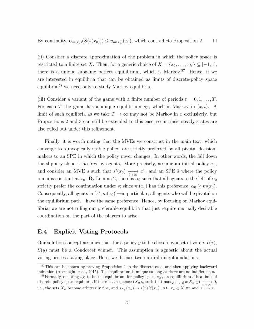
By continuity, Um(x0)(S(s(x0))) ≤ um(x0)(x0), which contradicts Proposition 2.

(ii) Consider a discrete approximation of the problem in which the policy space is

restricted to a finite set X. Then, for a generic choice of X = {x1, . . . , xN} ⊆ [−1, 1],

there is a unique subgame perfect equilibrium, which is Markov.57 Hence, if we

are interested in equilibria that can be obtained as limits of discrete-policy space

equilibria,58 we need only to study Markov equilibria.

(iii) Consider a variant of the game with a finite number of periods t = 0, 1, . . . , T .

For each T the game has a unique equilibrium sT , which is Markov in (x, t). A

limit of such equilibria as we take T → ∞ may not be Markov in x exclusively, but

Propositions 2 and 3 can still be extended to this case, so intrinsic steady states are

also ruled out under this refinement.

Finally, it is worth noting that the MVEs we construct in the main text, which

converge to a myopically stable policy, are strictly preferred by all pivotal decision-

makers to an SPE in which the policy never changes. In other words, the fall down

the slippery slope is desired by agents. More precisely, assume an initial policy x0,

and consider an MVE s such that st(x0) −−−→t→∞

x∗, and an SPE s where the policy

remains constant at x0. By Lemma 2, there is α0 such that all agents to the left of α0

strictly prefer the continuation under s; since m(x0) has this preference, α0 ≥ m(x0).

Consequently, all agents in [x∗,m(x0)]—in particular, all agents who will be pivotal on

the equilibrium path—have the same preference. Hence, by focusing on Markov equi-

libria, we are not ruling out preferable equilibria that just require mutually desirable

coordination on the part of the players to arise.

E.4 Explicit Voting Protocols

Our solution concept assumes that, for a policy y to be chosen by a set of voters I(x),

S(y) must be a Condorcet winner. This assumption is agnostic about the actual

voting process taking place. Here, we discuss two natural microfoundations.

57This can be shown by proving Proposition 1 in the discrete case, and then applying backwardinduction (Acemoglu et al., 2015). The equilibrium is unique so long as there are no indifferences.

58Formally, denoting sX to be the equilibrium for policy space sX , an equilibrium s is a limit ofdiscrete-policy space equilibria if there is a sequence (Xn)n such that maxy∈[−1,1] d(Xn, y) −−−−→

n→∞0,

i.e., the sets Xn become arbitrarily fine, and sXn(xn)→ s(x) ∀(xn)n s.t. xn ∈ Xn∀n and xn → x.

75

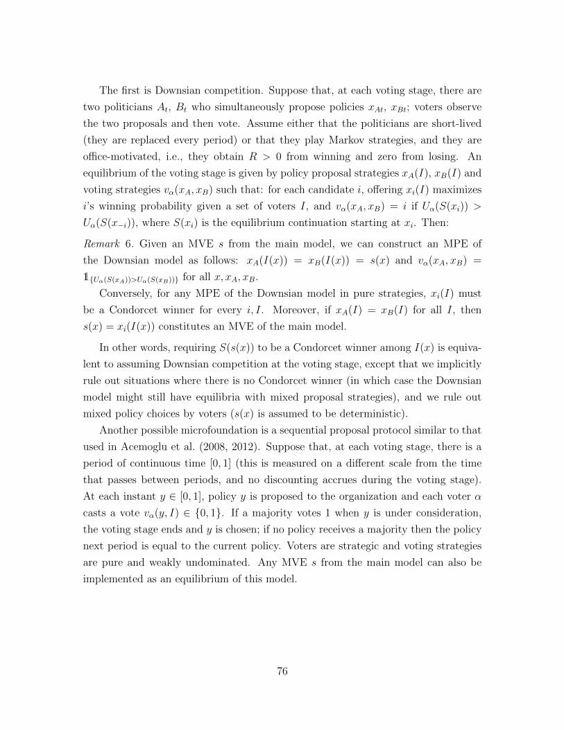
The first is Downsian competition. Suppose that, at each voting stage, there are

two politicians At, Bt who simultaneously propose policies xAt, xBt; voters observe

the two proposals and then vote. Assume either that the politicians are short-lived

(they are replaced every period) or that they play Markov strategies, and they are

office-motivated, i.e., they obtain R > 0 from winning and zero from losing. An

equilibrium of the voting stage is given by policy proposal strategies xA(I), xB(I) and

voting strategies vα(xA, xB) such that: for each candidate i, offering xi(I) maximizes

i’s winning probability given a set of voters I, and vα(xA, xB) = i if Uα(S(xi)) >

Uα(S(x−i)), where S(xi) is the equilibrium continuation starting at xi. Then:

Remark 6. Given an MVE s from the main model, we can construct an MPE of

the Downsian model as follows: xA(I(x)) = xB(I(x)) = s(x) and vα(xA, xB) =

1{Uα(S(xA))>Uα(S(xB))} for all x, xA, xB.

Conversely, for any MPE of the Downsian model in pure strategies, xi(I) must

be a Condorcet winner for every i, I. Moreover, if xA(I) = xB(I) for all I, then

s(x) = xi(I(x)) constitutes an MVE of the main model.

In other words, requiring S(s(x)) to be a Condorcet winner among I(x) is equiva-

lent to assuming Downsian competition at the voting stage, except that we implicitly

rule out situations where there is no Condorcet winner (in which case the Downsian

model might still have equilibria with mixed proposal strategies), and we rule out

mixed policy choices by voters (s(x) is assumed to be deterministic).

Another possible microfoundation is a sequential proposal protocol similar to that

used in Acemoglu et al. (2008, 2012). Suppose that, at each voting stage, there is a

period of continuous time [0, 1] (this is measured on a different scale from the time

that passes between periods, and no discounting accrues during the voting stage).

At each instant y ∈ [0, 1], policy y is proposed to the organization and each voter α

casts a vote vα(y, I) ∈ {0, 1}. If a majority votes 1 when y is under consideration,

the voting stage ends and y is chosen; if no policy receives a majority then the policy

next period is equal to the current policy. Voters are strategic and voting strategies

are pure and weakly undominated. Any MVE s from the main model can also be

implemented as an equilibrium of this model.

76