Policy Paper 28

Commodity Outlook on Major Cereals in India

Shinoj Parappurathu Anjani Kumar

Shiv Kumar Rajni Jain

National Centre for Agricultural Economics and Policy ResearchNew Delhi - 110 012

Commodity Outlook on Major Cereals in IndiaDr. Shinoj Parappurathu is Scientist with NCAP, New Delhi – 110012

Dr. Anjani Kumar is Principal Scientist (On deputation to IFPRI, New Delhi) with NCAP, New Delhi – 110012

Dr. Shiv Kumar is Principal Scientist with ICAR Headquarters, New Delhi – 110012

Dr. Rajni Jain is Principal Scientist with NCAP, New Delhi – 110012

Published

June, 2014

Published by

Dr. Ramesh Chand Director National Centre for Agricultural Economics and Policy Research New Delhi - 110 012

© 2014, NCAP, New Delhi

The views expressed by the authors in this policy paper are personal and do not necessarily reflect the official policy or position of the organization they represent.

Printed atVenus Printers and Publishers, B-62/8, Naraina Industrial Area, Phase II, New Delhi – 110 028, Phone No.: 011-45576780, 9810089097

ii

59

Acknowledgements

This Policy Paper is drawn from the project ‘Developing a Decision Support System for Commodity Market Outlook’ carried out at NCAP under the sponsorship of National Agricultural Innovation Project (NAIP) of the ICAR. The authors thank the ICAR and NAIP for the financial and technical assistance received for successful completion of the project. We express our profuse gratitude to Dr. Ramesh Chand, Director, NCAP and consortium Principal Investigator of the Project for his valuable guidance and support throughout the study. We are indebted to Dr. S.S. Acharya, former Chairman, CACP, Dr. Mruthyunjaya, former Director, NAIP and Dr. S.L. Mehta, former Vice Chancellor, MPUAT, Udaipur for extending their learned comments and feedback while reviewing the project activities. The guidance of Dr. P.K. Joshi, former Director, NCAP, during the initial stage of the project has been instrumental in taking the study to the present stage, and we gratefully acknowledge his contribution.The technical inputs and inspiring guidance extended by Dr. Praduman Kumar, former Head and Professor, Division of Agricultural Economics, IARI and consultant to the project is gratefully acknowledged. We also express our gratitude to Dr. Shashanka Bhide, Dr. Ganesh Kumar and Dr. P.S. Birthal, Senior Faculty at NCAER, IGIDR and NCAP respectively, for rendering their learned thoughts and suggestions during the various stages of the study. The motivating role played by Dr. Bangali Baboo, then Director, NAIP and Dr. N.T. Yaduraju, Dr. R.C. Agrawal, and Dr. P.S. Pandey, successive National Coordinators of NAIP, are worth mentioning. We wish to place on record, our profound gratitude to Dr. Kranti Mulik, Dr. Amani Elobeid and Dr. Miguel Carriquiry, Commodity Analysts at the Centre for Agricultural and Rural Development, Iowa State University, USA for their expert directions in shaping up the study results.The scholarlyguidance of Dr. William G. Tomek and Dr. K.V. Raman, Senior Faculty at Cornell University, USA during the initial stage of the study undertaken as part of the Borlaug Fellowship programme of the first author is gratefully acknowledged. A part of this Paper is published in the Journal, Margin-The Journal of Applied Economic Research, for which the authors are thankful to the SAGE Publications. The technical assistance received from RAs/SRFs of the project that included Tinu Joseph, Pankaj Sharma, Raj Kumar Rai, Arvider Kaur and Simmi Rana are duly accredited. Finally, the comments and suggestions received from the participants of various seminars/conferences organized under the project are also gratefully acknowledged.

Authors

iii

60

61v

Acronyms and Abbreviations

ABARES Australian Bureau of Agricultural and Resource Economics and Sciences

ADB Asian Development Bank

AGE Applied General Equilibrium

AIDS Almost Ideal Demand System

ARDL Auto Regressive Distributed Lag

CACP Commission for Agricultural Costs and Prices

CARD Centre for Agricultural and Rural Development

CCLS Country-Commodity Linked Modeling System

CGE Computable General Equilibrium

ERS Economic Research Service

ESIM European Simulation Model

EU European Union

FAO Food and Agriculture Organization

FAPRI Food and Agricultural Policy Research Institute

FAPSIM Food and Agricultural Policy Simulation Model

FCDS Food Characteristic Demand System

GDP Gross Domestic Product

GoI Government of India

ICAR Indian Council of Agricultural Research

IFPRI International Food Policy Research Institute

IGIDR Indira Gandhi Institute of Development Research

IMPACT The International Model for Policy Analysis of Agricultural Commodities and Trade

MAE Mean Absolute Error

MAPE Mean Absolute Percent Error

ML Maximum Likelihood

62

MSP Minimum Support Prices

NAIP National Agricultural Innovation Project

NCAER National Council for Applied Economic Research

OECD Organization for Economic Cooperation and Development

OLS Ordinary Least Squares

PSD Production, Supply, Distribution

QAIDS Quadratic Almost Ideal Demand System

2 SLS Two Stage Least Square

SURE Seemingly Unrelated Regression Equation

SWOPSIM Static World Simulation Model

USDA United States Department of Agriculture

WATSIM World Agricultural Trade Simulation Model

vi

Contents

Acknowledgements iii

Acronyms and Abbreviations v

List of Tables ix

List of Figures ix

List of Appendices ix

Executive Summary xi

1. Introduction 1

1.1. Background 1

1.2. Scope of the Paper 4

1.3. Organization of the Paper 4

2. Literature Review on Commodity Outlook 5

2.1. History of Commodity Outlook 5

2.2. Approaches of Commodity Outlook Modeling 6

2.2.1. Time Series versus Market Equilibrium Models 6

2.2.2. Comparative Static versus Dynamic Models 7

2.3. Review on Selected Outlook Models 7

2.3.1. Global Models 8

2.3.2. Country-specific Models 12

2.3.3. Indian Studies 13

2.4. Major Insights from the Review 17

3. Data and Methodology 18

3.1. The Data 18

3.2. Methodological Framework 18

3.3. Model Structure 19

vii

3.4. Simulations and Sensitivity Analysis 25

3.5. Validation of the Model 25

3.6. Limitations of the Model 26

4. Main Results and Discussion 28

4.1. National and Regional Outlooks 28

4.2. Simulation Results 32

5. Conclusions and Policy Implications 35

References 38

Appendices 42

viii

List of Tables

Table 3.1: Cereal Outlook Model: Commodity, spatial and 23 temporal dimensions

Table 3.2: Results of validation of the Cereal Outlook Model 26

Table 4.1: Outlook for wheat in India: 2010-11 to 2025-26 29

Table 4.2: Outlook for rice in India: 2010-11 to 2025-26 30

Table 4.3: Outlook for maize in India: 2010-11 to 2025-26 31

Table 4.4: Effects of sustained 2% annual increase in MSP 33 of wheat, rice and maize

Table 4.5: Effects of sustained 2% annual increase in cost 34 of cultivation of wheat, rice and maize

List of FiguresFigure 1: Modeling Framework of Cereal Outlook Model: 19

An illustration

List of AppendicesAppendix 1: Partial equilibrium models for agricultural 42

commodity outlook and policy simulations

Appendix 2: Cereal Outlook Model: Specifications 44

Appendix 3: Projected GDP, population and per capital income 53 in India: 2010-2025

Appendix 4: Market clearing prices at supply-demand 54 equilibrium for rice, wheat and maize

Appendix 5: Comparison of Cereal Outlook Model projections 55 with that of FAO/OECD and FAPRI-CARD models

ix

66x

67

Executive Summary

The emerging scenarios in agriculture and allied sectors highlight the increasing need for timely and reliable information on the likely demand, production, trade and prices of important food commodities. In a country like India, where attaining household level food security for a considerable section of the population still remains a challenge, advance information systems would not only help in efficient functioning of markets and food management systems, but also in targeting investments and efforts towards accelerating agricultural growth and conserving natural resources. India’s experiences in the ambit of food policy formulation so far shows that lack of relevant information that supports decision-making often leads to knee jerk reactions that create uncertainties in the market and are detrimental to the interests of producers, consumers and traders. This Policy Paper is an attempt in this direction that targets to put forth a decision support system which could generate outlooks on pertinent demand and supply side variables of major staple food crops in the country.

With the mandate of developing the above said decision support system, the study team commenced the activity with a detailed review of the existing systems at the national and international level that functions in the domain of commodity market outlook on important agricultural commodities. The review brought out the fact that there have been several attempts in the past that looked in detail into the demand and supply side dynamics of agricultural commodities which were useful both for generating future outlooks and in undertaking simulations under alternative policy scenarios. One of the pioneering attempts in this direction was undertaken jointly by the United Nations Commission on International Trade and the Food and Agriculture Organization (FAO) Committee on Commodity problems as early as in 1962. Since then, FAO continued to publish medium-term agricultural commodity projections at regular intervals. In the due course, several international and national organizations like Organization for Economic Cooperation and Development (OECD), International Food Policy Research Institute (IFPRI), United States Department of Agriculture (USDA), etc. ventured into this area and started disseminating independent outlooks on global as well as regional food situation. Some of the widely popular models include OECD-FAO annual Agricultural Outlook Model, USDA Agricultural Outlook Model, FAPRI-CARD model, European Simulation Model (ESIM), World Agricultural Trade Simulation Model (WATSIM) and so on. The International Model for Policy Analysis

xi

68

of Agricultural Commodities and Trade (IMPACT) of the IFPRI has been in use for undertaking policy simulations on global agricultural scenarios. In addition, there are several country specific models like the Irish Agricultural Model, agricultural outlook model of Australian Bureau of Agricultural and Resource Economics and Sciences (ABARES), South African wheat model, FAPRI model for Chinese meat sector, etc. Most of the above models were built to generate advance information on key policy variables related to the agricultural and allied sectors. For this reason, they have been playing a primary role in the academic and political debate on the effects of agricultural and trade policies at national and international level for quite some time. In India, though there have been limited institutional mechanisms that undertook regular and comprehensive commodity-specific outlooks, several scholarly studies carried out by individual researchers and organizations from time to time find place in the literature.The review concluded that, though the various attempts discussed above were made in response to specific academic requirements pertaining to the commodities and geographical areas which they catered to, there are several common features cutting across them. Broad similarities in terms of basic assumptions, modeling approach, functionalities, sectorial linkages, etc. could be noticed. Therefore, with suitable adaptations and modifications, such approaches could be followed and replicated for issue-based future use.

With the insights obtained from the review, the authors developed an India-specific model namely, Cereal Outlook Model on three major cereals, viz. rice, wheat and maize. This Model has the functionality for generating commodity outlooks based on four key components of the food balance sheet, viz. demand, supply, trade and prices. This Paper details on the theoretical underpinnings as well as practical applications of the Model, which is dynamic as well as built under a partial equilibrium framework, designed specifically for India-specific applications. With the Model, demand- and supply-side outlook on key variables such as area, yield, production, consumption and net trade of wheat, rice and maize have been attempted with projections extending up to 2025-26. The results were finalized after suitable calibrations based on the technical parameters and were subsequently validated using standard procedures. On the supply side, area, yield and production were modeled at the regional levels. For this, the country was divided into six regions, namely East, West, North, South, Hills and North-East and area and yield equations were fitted separately for each region under each crop. The estimates on production were obtained from the estimates on area and yield for each of these regions, and the national production estimates were computed by aggregating these regional estimates. On the demand side, the country was treated as

xii

69

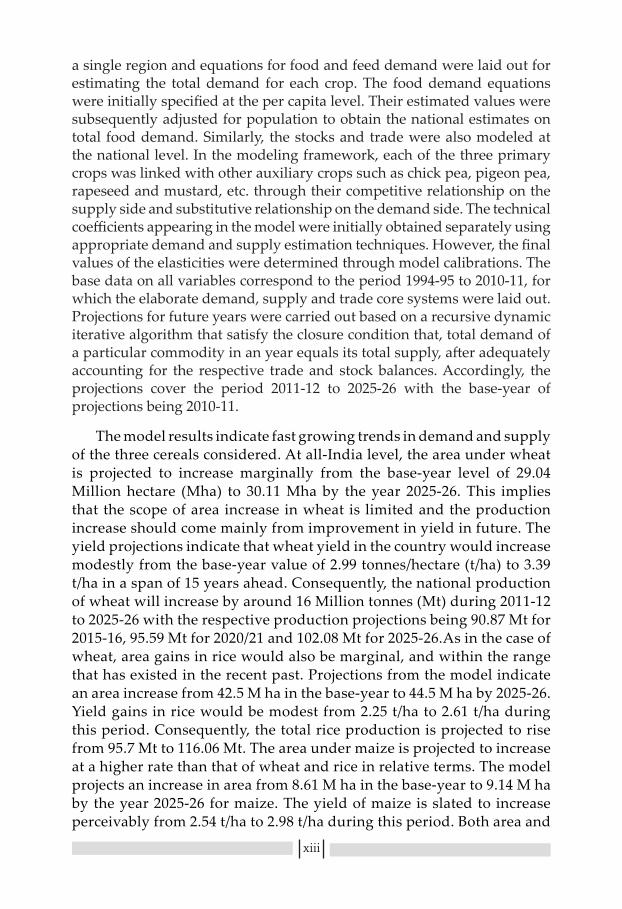
a single region and equations for food and feed demand were laid out for estimating the total demand for each crop. The food demand equations were initially specified at the per capita level. Their estimated values were subsequently adjusted for population to obtain the national estimates on total food demand. Similarly, the stocks and trade were also modeled at the national level. In the modeling framework, each of the three primary crops was linked with other auxiliary crops such as chick pea, pigeon pea, rapeseed and mustard, etc. through their competitive relationship on the supply side and substitutive relationship on the demand side. The technical coefficients appearing in the model were initially obtained separately using appropriate demand and supply estimation techniques. However, the final values of the elasticities were determined through model calibrations. The base data on all variables correspond to the period 1994-95 to 2010-11, for which the elaborate demand, supply and trade core systems were laid out. Projections for future years were carried out based on a recursive dynamic iterative algorithm that satisfy the closure condition that, total demand of a particular commodity in an year equals its total supply, after adequately accounting for the respective trade and stock balances. Accordingly, the projections cover the period 2011-12 to 2025-26 with the base-year of projections being 2010-11.

The model results indicate fast growing trends in demand and supply of the three cereals considered. At all-India level, the area under wheat is projected to increase marginally from the base-year level of 29.04 Million hectare (Mha) to 30.11 Mha by the year 2025-26. This implies that the scope of area increase in wheat is limited and the production increase should come mainly from improvement in yield in future. The yield projections indicate that wheat yield in the country would increase modestly from the base-year value of 2.99 tonnes/hectare (t/ha) to 3.39 t/ha in a span of 15 years ahead. Consequently, the national production of wheat will increase by around 16 Million tonnes (Mt) during 2011-12 to 2025-26 with the respective production projections being 90.87 Mt for 2015-16, 95.59 Mt for 2020/21 and 102.08 Mt for 2025-26.As in the case of wheat, area gains in rice would also be marginal, and within the range that has existed in the recent past. Projections from the model indicate an area increase from 42.5 M ha in the base-year to 44.5 M ha by 2025-26. Yield gains in rice would be modest from 2.25 t/ha to 2.61 t/ha during this period. Consequently, the total rice production is projected to rise from 95.7 Mt to 116.06 Mt. The area under maize is projected to increase at a higher rate than that of wheat and rice in relative terms. The model projects an increase in area from 8.61 M ha in the base-year to 9.14 M ha by the year 2025-26 for maize. The yield of maize is slated to increase perceivably from 2.54 t/ha to 2.98 t/ha during this period. Both area and

xiii

70

yield gains would result in the increase of maize production from 21.8 Mt to 27.19 Mt between the base-year and terminal year of projections. Such gains in production would be appreciable for a marginal crop like maize, and indicate the future potential of this important low value staple crop.

Apart from generating outlooks, the model has also been designed for undertaking simulations under alternative policy scenarios, a utility that may help the policy makers in evaluating the implications of alternative policy decisions and changes in the market dynamics. The simulation results corresponding to two scenarios of sustained increase in MSP and cost of cultivation of the three crops were consistent with intuitive hypotheses. The first one, which corresponds to a sustained 2 per cent real annual increase in MSP of wheat, rice and maize resulted in increase of area, production, consumption as well as net trade in all three commodities. The results showed that, area under rice, wheat and maize would increase consistently over the years to reach at 1.68 per cent, 2.50 per cent and 2.36 per cent respectively by the year 2025-26 over the base-year. Increase in MSP, was also associated with increase in production, consumption as well as net trade in all three commodities. Similarly, the simulations with respect to sustained increase in cost of cultivation resulted in decline of area, production, consumption and net trade in all commodities considered. In case of wheat, the reduction of area would be to the tune of 0.08 per cent from the base-line by the year 2025-26. Area reduction in rice would be at 0.02 per cent in relation to baseline, where as there would be negligible effects on maize area. Lower area under cultivation would therein result lower production as confirmed by the simulation results. The corresponding decline in production of wheat, rice and maize would be at 0.21 per cent, 0.13 per cent and 0.13 per cent respectively by the year 2025-26. Equivalent squeeze in consumption as well as net trade would also follow in the course of time due to lower area and production of the cereals under consideration. In nutshell, the Paper threw light on a time tested, but relatively less explored approach to derive future outlooks on important staple crops that could have significant say in the country’s food security in times to come.

xiv

1

Introduction

1.1. Background

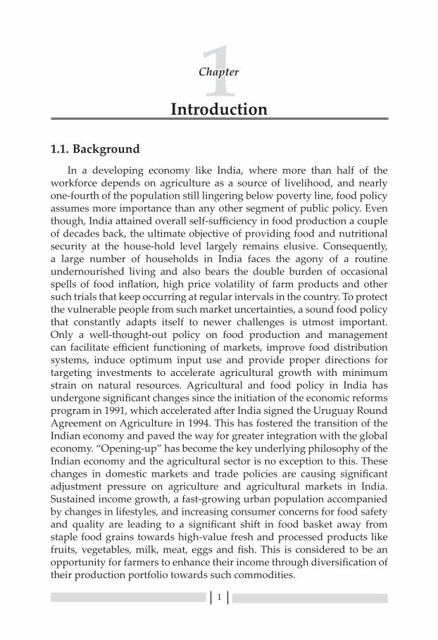
In a developing economy like India, where more than half of the workforce depends on agriculture as a source of livelihood, and nearly one-fourth of the population still lingering below poverty line, food policy assumes more importance than any other segment of public policy. Even though, India attained overall self-sufficiency in food production a couple of decades back, the ultimate objective of providing food and nutritional security at the house-hold level largely remains elusive. Consequently, a large number of households in India faces the agony of a routine undernourished living and also bears the double burden of occasional spells of food inflation, high price volatility of farm products and other such trials that keep occurring at regular intervals in the country. To protect the vulnerable people from such market uncertainties, a sound food policy that constantly adapts itself to newer challenges is utmost important. Only a well-thought-out policy on food production and management can facilitate efficient functioning of markets, improve food distribution systems, induce optimum input use and provide proper directions for targeting investments to accelerate agricultural growth with minimum strain on natural resources. Agricultural and food policy in India has undergone significant changes since the initiation of the economic reforms program in 1991, which accelerated after India signed the Uruguay Round Agreement on Agriculture in 1994. This has fostered the transition of the Indian economy and paved the way for greater integration with the global economy. “Opening-up” has become the key underlying philosophy of the Indian economy and the agricultural sector is no exception to this. These changes in domestic markets and trade policies are causing significant adjustment pressure on agriculture and agricultural markets in India. Sustained income growth, a fast-growing urban population accompanied by changes in lifestyles, and increasing consumer concerns for food safety and quality are leading to a significant shift in food basket away from staple food grains towards high-value fresh and processed products like fruits, vegetables, milk, meat, eggs and fish. This is considered to be an opportunity for farmers to enhance their income through diversification of their production portfolio towards such commodities.

1

2

Opening up of domestic markets to global competition throws both opportunities as well as challenges for India. Globalization of agri-food markets provides opportunities to farmers to improve their competitiveness for greater participation in international trade. However, opening up is also accompanied by a threat of cheap imports and high volatility in food prices. The recent episodes of high food inflation coupled with extraordinary price variability in major staple food cereals, fruits and vegetables are ample testimony to the emerging food market situation in the country. The evolving agriculture and food marketing scenarios indicate an increasing need for timely and reliable information on key aspects related to food production and its management in the domestic market. In this regard, reliable and advance estimates on medium- and long-term demand, supply, trade and prices of important food commodities forms an essential basis for planning. Absence of such relevant information to support decision-making often leads to knee jerk reactions that create uncertainty in the market and proves detrimental to the interest of producers, consumers and the government.

There have been several sporadic attempts in the past, particularly after the inception of planned development, to project future demand and supply of food and agricultural commodities using alternative methodological approaches. For instance, the National Commission on Agriculture in India (1976) did extensive exercises on demand estimation and projections. On similar lines, the Planning Commission, Government of India undertakes regular exercises of projecting demand and supply of major food commodities to enable realistic target-setting on food production in successive plans. Scholarly articles by individual researchers and organizations with short-/medium-/long-term projections on demand, supply, prices etc. also find place in the literature from time to time. Some recent studies include Radha krishna and Ravi (1994); Kumar (1998); Bhalla et al. (1999);Paroda and Kumar (2000); Dastagiri (2004); Mythili (2006); Mittal (2008); Chand (2007; 2009); Kumar et al. (2009; 2010) etc. In similar lines, the National Council of Applied Economics Research (NCAER) has recently started publishing a series on ‘Agricultural Outlook and Situation Analysis Reports’ (NCAER, 2013) that covers semi-annual and medium-term outlooks on food supply and demand conditions on major food as well as commercial crops in India. Another on-going initiative namely Forecasting Agriculture Outputs through Satellite, Agrometeorology and Land based observations (FASAL) co-ordinated by the Ministry of Agriculture and Cooperation, Government of India (GoI) undertakes short-term forecasts on production of major crops based on a multi-disciplinary approach. However, only a few of the above studies/institutional initiatives looked at the food balance sheet in its entirety while undertaking projections. Some of these studies

3

focused on projections of demand, and others on supply, and those studies which looked at both did not see how well they balanced so that the other components of the balance sheet could be reasonably explained. Moreover, models used by these studies were not sophisticated enough to undertake scenario analysis under varying policy and technology settings. With increasing integration of India’s economy with rest of the world, it has become more and more complicated to predict the effects of changes in the global markets on domestic producers and consumers. India’s domestic agricultural and trade policies have been evolving constantly to adjust to the frequent changes in the international markets, and this has brought in certain amount of uncertainty in its predictability. Therefore, along with the capacity to undertake projections, it is also desirable to have systems in place to carry out scenario analyses to assist in decision making.

Recognizing the need for regular outlooks on future demand, supply and trade of food commodities, many international organizations and national policy research institutes in developed countries have been showing great interest in maintaining economic applications that can serve this purpose. The United States Department of Agriculture (USDA) has a strong program on developing future outlooks (both global and domestic), which provide short-term and long-term projections for important agricultural commodities. Similarly, Food and Agriculture Organization (FAO) of United Nations, World Bank and Asian Development Bank (ADB) provide global as well as country-specific medium-term demand, production, trade and price prospects of major agricultural commodities. These international programs take inputs from econometric modeling solutions that can realistically capture the emergent demand-supply scenarios with the help of complex modeling algorithms. Such models are commonly known as commodity outlook models and are generally built either under partial equilibrium or computable general equilibrium (CGE) framework1. Outlook models commonly serve the dual role of generating future projections on key variables as well as undertaking simulations under alternative scenarios. In India, even though several scholars have used CGE modeling techniques for economic policy analysis including that pertaining to agricultural sector (Parikh et al, 1995, 2003; Kumar, 1992), the use of outlook models specific to agricultural commodities has been rather limited. Keeping this in view, this Policy Paper discusses the applications of a partial equilibrium modeling framework developed by the authors with the specific purpose of generating commodity outlook

1Partial equilibrium models focus only at the demand and supply dynamics of a particular sector with the underlying assumption of Ceteris paribus for other sectors in the economy, whereas, general equilibrium models are economy-wide models with many interacting sectors, and with the assumption of Mutatis mutandis.

4

for major cereals in India (Cereal Outlook Model here onwards). Cereals including rice, wheat and maize were chosen for this purpose owing to their overwhelming role in maintaining the food and nutritional security of multitude of domestic consumers in the country. Moreover, these three cereals occupy a substantial share of cropped area in the country and are most frequently depended upon to cater to the calorific requirements of majority of vulnerable sections of the economy. In this backdrop, the Paper addresses the need for advance information on variables and factors that are related to the above three staple commodities which in turn would contribute to the pool of intelligence based on which food policy in the country is drawn and applied in practice.

1.2. Scope of the Paper

The paper primarily focuses on the methodological underpinnings as well as practical applications of the Cereal Outlook Model that was developed based on the best of available information from the literature and expertise available with the research team. It goes on to present the projections on supply and demand side variables of the three selected cereals in the medium- and long-term. On the supply side, major variables like area, yield, production, etc. were addressed whereas on the demand side, household food demand, demand for feed, other uses demand, etc. were dealt with. Stock and trade aspects were also covered as the underlying model was ‘open’ in time and space. Both national and regional dimensions were included for projections so as to capture the supply and demand diversities present across the country. The results of simulation exercises carried out based on a few scenarios with changes in key exogenous variables and their impacts on the projections were also discussed at the end.

1.3. Organization of the Paper

This Policy Paper has been organized in five chapters including the Introduction. A brief review on various national and international commodity outlook models, their theoretical affiliations and practical applications available in the literature were discussed in chapter 2. The third chapter presents the data and methodology used in the present study. The main results derived from the Cereal Outlook Model in the form of projections on key variables and their practical interpretations along with a few scenario analyses based on policy simulations were presented in Chapter 4. Finally, conclusions and policy implications derived based on the modeling work have been presented in the last chapter.

5

Literature Review on Commodity Outlook

2.1. History of Commodity Outlook

Agricultural commodity outlook modeling has a long history of its own. Robert Malthus with his masterpiece “An Essay on the Principle of Population” in 1798 is believed to be the first to analyze the world food concerns into a formal ‘model’. Malthusian concern was mainly on population growth and land constraints for meeting the future demand of agricultural commodities. Overtime, the understanding of the global food security became complex. Population projections and land constraints were not enough to forecast the demand and supply of food grains. After World War II, the focus shifted to a requirements approach where minimum nutritional needs of representative individuals, stratified by geography, sex, and age were estimated based on consumption levels and population growth (Mc Calla and Revoredo, 2001). Later, the FAO adopted the food demand based approach for forecasting global food demand which was fortified with the use of income and price elasticity estimates. The first systematic attempt to prepare agricultural commodity projections was made in 1962 jointly by the United Nations Commission on International Trade and the FAO Committee on Commodity problems. Since then, FAO continued to publish medium-term agricultural commodity projections at regular intervals. In the due course, several international and national organizations like Organization for Economic Cooperation and Development (OECD), International Food Policy Research Institute (IFPRI), United States Department of Agriculture (USDA), etc. ventured into this area and started disseminating independent outlooks on global as well as regional food situation. Some of the widely popular models presently in use include OECD-FAO annual Agricultural Outlook Model prepared jointly by FAO and OECD; USDA Agricultural Outlook Model; FAPRI-CARD model designed jointly by Food and Agricultural Policy Research Institute (FAPRI) and Centre for Agricultural and Rural Development (CARD) based in Iowa State University, USA; European Simulation Model (ESIM) developed by the Institute of Agricultural Economics, University of Gottingen in collaboration with Economic Research Service (ERS) of USDA; World Agricultural Trade Simulation Model (WATSIM) developed and maintained by the Institute of Agricultural Policy, Bonn University

2

6

and so on. The International Model for Policy Analysis of Agricultural Commodities and Trade (IMPACT) of IFPRI has been in use for undertaking policy simulations on global agricultural scenarios. In addition, there are several country specific models like Irish Agricultural Model, agricultural outlook model of Australian Bureau of Agricultural and Resource Economics and Sciences (ABARES), South African wheat model, FAPRI model for Chinese meat sector, etc. Most of the above models were built to generate advance information on key policy variables related to the agricultural and allied sectors. For this reason, they have been playing a primary role in the academic and political debate on the effects of agricultural and trade policies at national and international level for quite some time.

2.2. Approaches to Commodity Outlook Modeling

Based on the underlying assumptions, method of attainment of equilibrium, nature of data required, etc. agricultural commodity outlook models can be classified into several broad categories as outlined below;

2.2.1. Time Series versus Market Equilibrium Models

Time series projection models try to forecast the future through extrapolation of historical data. They put more importance to statistical behavior of historical data rather than on the economic theory behind behavioral equations. On the other hand, market equilibrium models contain the behavior of economic agents to changes in input and output prices as well as other structural supply and demand shifters. The objective is to determine equilibrium prices and quantities on sets of markets. In a fully fledged global equilibrium model, endogenous prices are attached to world markets as well as domestic markets. These types of models assume that behavioral response of suppliers and buyers is derived from optimizing assumptions. Also, standard assumptions include constant returns of technology, homothetic preferences, and perfect competitive market. The optimization process is usually not modeled explicitly but demand and supply are specified as functions of income, prices and elasticities (Tongeren et al, 1999). On the assumptions of flexibility of production factors, equilibrium models can be classified into short term, medium term and long term models. In the short term, production factors such as capital, land and labor are fixed, and are not allowed to reallocate between alternative users. Medium term models allow reallocation of all production factors as response to some exogenous events. Long term models also model exogenous capital formation. Market equilibrium models can be classified further as partial equilibrium as well as economy-wide models.

7

Partial equilibrium models consider agricultural system as a closed system without linkages with the rest of the economy. Partial equilibrium models focus only at the demand and supply dynamics of a particular sector with the underlying assumption of ceteris paribus for other sectors in the economy. Partial models may be single or multi-commodity. Multi-commodity models capture supply and demand interrelationships among a set of agricultural products. Partial equilibrium models include linear or log-linear behavioral equations allowing representation of supply and demand relationships. They also incorporate exogenous variables such as technical change, world population and household income into their supply and demand relationships. In contrast, economy-wide models (general equilibrium models) provide complete representation of national economies with the assumption of mutatis mutandis (Alston et al, 1998). They capture implications of international trade for the economy as a whole, covering the circular flow of income and expenditure and taking care of inter-industry relationships. The major classes of economy-wide models include macro-economic models, input-output models and Applied General Equilibrium (AGE) models. AGE models also contain full input-output detail but mainly behavioral equations of responses of producers, consumers, importers and exporters and other agents of the economy. They are specifically concerned with resource allocation issues.

2.2.2. Comparative Static Models versus Dynamic ModelsThe comparative static approach studies the difference between

equilibriums resulting from different assumptions on exogenous data or policy variables. Here, the time path between equilibriums is ignored. But dynamic models allow the analysis of lagged transmissions and adjustment process overtime. Dynamic models can be used to trace the accumulation of stock variables and in static models policy changes have no effect on accumulation of stocks (Gujarati, 2003). The most frequently used dynamic approach is a recursive sequence of temporary equilibriums, i.e., in each time period, the model is solved for equilibrium, given the exogenous conditions prevailing for that particular period. Recursive models do not guarantee time-consistent behavior. Comparative static models are usually used to generate projections of policy impacts at some future point of time achieved by constructing an artificial future data set consistent with the model’s assumptions called baseline and subsequently conducting a policy experiment on the basis of this projected dataset (Alston et al, 1998).

2.3. Review on Selected Outlook Models

As discussed above, there are several agricultural outlook models presently in vogue that are mainly used to predict future agricultural

8

situation. These models differ from one another in terms of basic objectives, model design, underlying assumptions, number of commodities and countries modeled, etc. To have a better understanding on these models, a concise review on some of the selected ones is detailed below;

2.3.1. Global Models

Early global models for commodity outlook developed by organizations such as FAO, IFPRI, OECD and USDA were trend projection models. They projected gaps or surpluses at regional and global levels by simply adding up surpluses and shortages of food grains. Prices in this model were assumed to be constant. These types of models give point estimates for the future. Spatial models (transportation model) which were developed later estimated actual trade flows over geographical regions by estimating the country’s surplus or shortage into a model that minimizes the cost of moving surplus to shortage locations. Another type is non-spatial price equilibrium global trade models and they estimated supply and demand functions for each country. The country functions were subsequently aggregated to form a world market system where prices will adjust until global supply equals global demand. Recursive/dynamic models, which are latest in this row, comes out with dynamic estimates for year after year that moves recursively towards the end point with requisite adjustments in its path. The ensuing section provides a cross comparison between some of the widely popular models such as OECD-FAO annual Agricultural Outlook Model, USDA Agricultural Outlook Model, FAPRI-CARD model, ESIM, WATSIM, IFPRI-IMPACT model, etc.

OECD-FAO Agricultural Outlook Model

The OECD-FAO Agricultural Outlook is model built under a partial equilibrium framework. This effort was started by OECD in the early 1990’s through the development of its AGLINK model-an economic model of world agriculture with detailed agriculture sector representation of OECD countries as well as Argentina, Brazil, China and Russia. Since 2004, this modeling system was greatly enhanced through the development of a similar agricultural model by FAO, named COSIMO, representing agricultural sectors in a large number of developing countries. The AGLINK-COSIMO modeling system is presently one of the most comprehensive partial equilibrium models for global agriculture. This modeling system is recursive dynamic in nature that includes land allocation along with demand-supply functions of agricultural commodities. The model is one of the tools used in the generation of baseline projections underlying the OECD-FAO Agricultural Outlook. For many countries, agricultural policies are specifically modeled within AGLINK-COSIMO. Along with

9

annual medium term outlook, OECD-FAO model is designed to conduct quantitative analysis of agricultural policies on principal agricultural markets (OECD/FAO, 2011; Lampe, 1998). Presently, the system includes 39 countries with 19 sub regions and derives outlook on 38 agricultural commodities.

USDA Agricultural Outlook Model

The USDA Agricultural outlook program takes inputs from a set of economic models including, a domestic crop-area allocation model, Food and Agricultural Policy Simulator (FAPSIM) model and the Country–Commodity Linked Modeling System (CCLS). The CCLS is maintained by the ERS of the USDA and is a large-scale dynamic partial equilibrium system consisting of 43 country and regional models. The FAPSIM is an annual econometric model of the U.S. agricultural sector. The USDA originally developed the model during the early 1980’s. Since that time, FAPSIM has been continually re-estimated and re-specified to reflect changes in the structure of the U.S. food and agricultural sector. The equations incorporated in the model are dynamic in nature reflecting the policies related to tariff, subsidies and trade restrictions. For the most part, FAPSIM uses a linear relationship to approximate the general functional form for each behavioral relationship. All parameters in the linear behavioral relationships were estimated by single equation regression methods. The large size of the model precludes the use of econometric methods designed for systems of equations (ERS, 2013). The country models in CCLS estimates production, consumption, stock and prices of agricultural commodities and they are integrated through trade and international reference prices. The USDA agricultural outlook program comes out with its outlook estimates every year with detailed outlook on the US agriculture as well as broad projections for the countries included in the program.

FAPRI-CARD Model

The FAPRI-CARD model mainly focuses on US agricultural commodities and their linkages with other countries (FAPRI, 2004). It is a wide inter-linked modeling system that incorporates simultaneous equations for demand, supply and trade dimensions of major agricultural commodities. It was originally developed by the Food and Agricultural Policy Research institute (FAPRI) of the Iowa State University, with the aim of modeling United States agriculture. Since then, the system has undergone progressive expansion with the co-operation of other US and foreign Universities. Each year the system produces a ten-year baseline for US and world agriculture, and is used extensively to simulate the effects of short- and medium-term changes in domestic agricultural and

10

trade policy. The standard FAPRI-CARD model includes twenty-four products and twenty-nine regions. Both these, however, can change with the specific sub-models, especially depending on the importance of the specific areas for the markets of a given product (Conforti, 2001). The model is partly dynamic, and includes lagged variables and partial adjustment mechanisms in several supply components. The individual commodity components are integrated into a larger system with other commodity components through price linkages that permit cross-commodity and cross-county interactions. The linkages between countries and commodities ultimately arrive into a market clearing equilibrium with a price determination process. Equilibrium prices, quantities, and net trade are determined by equating excess demands and supplies across regions and linking prices in each region to world prices. It includes macro-economic assumptions, farm policy assumptions and yield assumptions of the regions. Respect for theoretical restrictions appears to vary widely among the parts of the system, accordance with to the functional forms. The most frequently imposed properties are homogeneity and symmetry, while adding-up and curvature conditions are less frequent. Parameters are mostly based on ad hoc econometric estimates, based on simultaneous equation systems or, more frequently, on single equations. Methods of estimation also seem to change with different parts of the system, from Ordinary Least Squares (OLS) to non-linear iterative methods allowing for maximum likelihood (ML) estimates (Devadoss et al., 1989; 1993).

European Simulation Model (ESIM)

The ESIM was developed by the Institute of Agricultural Economics, University of Gottingen, Germany in collaboration with the Economic Research Service (ERS) of the USDA. It is a comparative static model with special emphasis to Central and Eastern European countries (Tongeren et al, 2001). The primary objective of the Model is to analyze the various EU policies on agricultural and allied sectors. The Model includes seven Central and Eastern European countries and the ‘rest of the world’ as a single region. The products considered include 27 different agricultural as well as livestock commodities that covers grains, oil seeds, processed oil seed products, feeds, dairy products, meat, sugar, egg, etc. The land allocation mechanism appears to be one of the most interesting features of the Model, together with theoretical restrictions and definition of domestic prices (Conforti, 2001). Rather than regular outlooks on commodities included, the focus of ESIM is primarily on simulation analysis that feeds its notable results to policy making process in the European Union (EU).

11

The World Agricultural Trade Simulation System (WATSIM)

The WATSIM model was developed based on the SPEL TRADE model of the Institute of Agricultural Policy, Bonn University. It is a group of two sub-models designed to project and simulate the developments on world agricultural markets. The medium-term policy simulation model is concerned with the impacts of agricultural policies with respect to trade restrictions and domestic measures on agricultural production, demand, trade and prices. Changes in natural and socio-economic conditions such as land availability and income growth were taken into consideration in the long-term policy simulation model. Most of the price and income elasticities were taken from Static World Simulation Model (SWOPSIM) framework of the USDA. The WATSIM model comprises of 15 regions with 29 products including crops and livestock. It is a comparative static, non-stochastic, non-spatial (bilateral trade are not modeled) partial equilibrium model. The world markets for agricultural products come to disequilibrium, if supply and demand exogenously moves away from their base year values. Changes in policies cause further imbalances in the process. The equilibrium algorithm in the model searches for new world market prices, transmitted into regional markets that cause the adjustments in supply and demand necessary to bring world market back to equilibrium (Lampe, 1998).

IFPRI IMPACT Model

The IMPACT model developed by the IFPRI encompasses policy analysis on global food demand, supply, trade and prices and their linkages with various bioenergy, climate change and diversification scenarios (Rosegrant et al., 2012). Within each country or region sub-model, supply, demand and prices for agricultural commodities are determined. These country and regional agricultural sub-models are linked through trade. Supply and demand functions incorporate supply and demand elasticities to approximate the underlying production and demand functions. World agricultural commodity prices are determined annually at levels that clear international markets. The model consists of 115 countries and 38 commodities and a water component that comprises of 126 water basins and a nutrition component representing 115 countries. All the major sectors of agriculture like poultry, dairy and livestock sector, fisheries sector and crop sector are given adequate representation. However, the IMPACT model is not suitable for short to medium-term projections unlike other commodity outlook models. It is more designed to derive policy simulations relating to food, environment, energy, land and water sectors that could be used for policy decisions pertaining to global agriculture.

12

ERS/PENN State Trade Model

It is a multi-commodity, multi-region and non-spatial, applied partial equilibrium model of agricultural policy and international agricultural trade. The Model was developed jointly by the ERS of the USDA and Penn State University, Pennsylvania, USA. The primary purpose of the Model is to undertake simulation exercises on global policy variables with special emphasis to international agricultural trade. Twelve countries/regions were chosen based on their interest to the agricultural situation of the United States. Thirty five commodities which include thirteen crops, twelve oil seeds products, four livestock products and six processed dairy products are included in the Model. The Model is a comparative static analysis tool to analyze scenarios that involve multi-year process of policy change. It uses Nerlovian partial adjustment factors to track short-term responses in production. Along with the output sector, the input sector (feed sector) has also been incorporated. The behavioral equations in the Model are mostly laid out in constant elasticity form (Stout and Abler, 2004).

Arkansans Global Rice Model

The Global Rice Model was developed with a view to undertake projections on global rice economy for policy, technology and structural market analysis. The Model was developed by the agricultural division of the Arkansas State University, USA in collaboration with the FAPRI. The parameters include global rice consumption, production, trade and prices. Twenty five major rice producing countries all over the world are included in this Model. It comes out with supply and utilization status, projection on area, yield, production, consumption, trade and stock of rice in the global scenario. Separate projections on various US states by rice type are also given (Wailes, 2004; Frank et al, 2004).

2.3.2. Country specific Models

Apart from the global models discussed above, some country specific models that are presently used or were recently in use for representing the food situation in individual countries are described below;

Meyner, et al., (2003) developed an econometric model to make baseline projections for supply and use of wheat in South Africa to analyze the impact of various policy alternatives on the wheat sector for the period 2002–08. The wheat model consists of three blocks namely, the supply block, the demand block and the price linkage block. On the supply block, the decisions of the producer to the size of planted area is influenced by producer price of wheat, input prices, producer prices of substitutes and complements, weather conditions and previous year’s area planted. The

13

yield in the model is linked to weather conditions that in turn determine the total production of the crop. The total supply of wheat is estimated by adding the beginning stock and total imports to the total production of the country. Imports are determined by both world price of wheat and local production. Human consumption, feed and seed consumption, exports and ending stocks determine the total demand for wheat in South Africa. A price linkage block allows the interaction between supply and demand block and links the world price to the local producer price, which in turn is linked to the local consumer price. Local prices of wheat are influenced by world prices. OLS was used to estimate single equations, which are collapsed into one system and estimated simultaneously using Two-Stage-Least Squares (2 SLS) estimation method. After the validation of the model’s performance it was used to make baseline projections.

To model the meat and egg sectors in China, FAPRI developed an outlook model that can generate annual projections. The Model consists of a demand system, a set of production equations, trade relationships and domestic market clearing conditions. The meat and egg production levels generated by this Model were used to calculate the demand for feed grains in China. The Model determines the expenditure for meat and an Almost Ideal Demand System (AIDS) is used to allocate the consumers’ meat budget to beef, pork, poultry and sheep meat purchases. The egg demand is determined by a modified linear equation. Per capita egg consumption is a function of the logarithm of the retail egg price, deflated by the stone price index for meat, and per capita real income. The closure condition that supply must equal demand plus net exports determines the equilibrium domestic prices in the Model (Frank, 1997).

The Irish Agricultural model was born out of the FAPRI-Ireland partnership and was developed primarily for agricultural policy analysis (Binfield et al, 2000). This Model is a standard recursive, dynamic, partial equilibrium model for the agricultural sector in Ireland. The Model was specified in an Auto Regressive Distributed Lag (ARDL) form. The model has provisions to link with the rest of the Europe. It undertakes 10 years projections for the key variables within each of the main agricultural commodities under two scenarios, viz., baseline or no policy change and a simulated scenario. The commodity covered includes cereals, diary, poultry, beef, sheep, pigs and inputs.

2.3.3. Indian Studies

Given the limited institutional mechanisms that bring out regular outlooks on important agricultural commodities, policy makers often depend on scholarly studies carried out by individual researchers and

14

organizations for obtaining inputs on possible future demand-supply, trade and price scenarios on selected commodities from time to time. Some such selected studies that find place in the literature are outlined below;

Kannan and Chakrabarty (1983) made an effort to project consumer demand for rice, wheat, pulses, edible oil, milk, meat, egg and fish in India for the period 1985-86 to 2000-01. This study was based on the estimates of expenditure elasticities. Selection of demand function was based on considering the historical changes in consumer preference in response to changes in level and distribution of income. Three types of functions were set with a breakdown of base period consumption between urban and rural population in India. A log-inverse function for cereals, a semi-log function for pulses, sugar, milk and edible oil and a double-log function for meat, fish and egg based on FAOs methodological notes were used for obtaining the projections.

Narain, et al. (1985) had estimated the projections on production of rice, wheat, jowar, maize, bajra and pulses for the year 1990. A crop-wise production function was fit relating to productivity of crop with proportion of irrigated area devoted to that crop, proportion of area under high yielding variety to total cultivated area under the crop and total consumption of nutrient per unit gross area under the crop. It was found that fertilizers, proportion of high yielding varieties to the total cropped area and proportion of irrigated area devoted to the crop were the main variables that affected crop productivity in case of rice and wheat. Weather was found to have an important role in determining the pulses production.

Kumar (1998) has worked out demand projections for food, for the years, 1995, 2000, 2010 and 2020 at constant prices (1987-88) using Food Characteristic Demand System (FCDS) model by accounting for urbanization, regional variation in consumption pattern, shifts in dietary pattern, income distribution, energy requirements and changes in taste and preferences of consumer food varieties. The study projected demand under alternative GDP growth at 4, 5 and 7 per cent levels.

Bhalla, et al. (1999) in their IFPRI discussion paper projected the cereal supply and demand under different scenarios for the year 2020. Cereal demand projections were based on the assumptions about growth in population, urbanization, and national per capita income as well as changes in consumption behavior, distribution of income, and livestock production systems. Baseline projections on per capita income and consumption expenditures were estimated from the National Sample Survey. The study has estimated the total cereal demand in 2020 with different scenarios such

15

as with 2 percent, 3.7 percent and 6 percent per capita income growth rate. The future growth in supply of cereals was analyzed by extending the use of inputs that has been proven successful in the past such as irrigation, modern varieties and fertilizers. The study has forecasted the supply of cereals for 2020 with different scenarios such as with additional land degradation, with reduced land degradation, increase in fertilizer consumption and irrigation and with genetic and technical efficiency improvements. The results of this analysis show that India may need 300 million tonnes of cereals by the year 2020.

Paroda and Kumar (2000) have studied the prevailing situation and trends in food production, food consumption pattern in South Asia and projected domestic demand for food grains, livestock, fisheries and horticultural products between the year 2000 and 2030.The study also fixed yield and production targets to maintain self-reliance status by different countries including India and suggested strategies for enhancing food production. They used FCDS model for estimation of consumer demand elasticities. The analysis has revealed that public investment in infrastructure, research and extension during the green revolution period had significantly helped the expansion of food production and diversified the consumers’ food basket. It underscored the fact that food demand challenges ahead are formidable, considering the non-availability of favorable factors of past growth, declining factor productivity in major cropping systems, and rapidly shrinking resource base. The study however suggested various production enhancing strategies considering the vast agricultural potential that still remains underutilized in the region.

Datta and Rajaraman (2003) undertook short-term forecasting of agricultural output at the state level using a time-series modeling framework. A univariate ARIMA model with data spanning from early 1950s till 2000 was fitted to obtain the forecast. The model incorporates the rainfall adequacy factor, a key determinant for short-term fluctuations in agricultural output. Projections were limited to three years in advance (up to 2002-03)and covered five states: Punjab, Rajasthan, Karnataka, Andhra Pradesh and Uttar Pradesh.

Dastagiri (2004) estimated the demand projections for livestock products in India for 2010 and 2020. A Seemingly Unrelated Regression Equation (SURE) model was used to estimate the price and income elasticities of demand which were subsequently used in projections. The major commodities for which projections were carried out included milk, mutton, chicken and eggs. The demand projections were carried out using the simple growth model utilizing the estimated expenditure elasticities, population and per capita income growth rates and urbanization.

16

Mittal (2008) has projected the demand and supply trends of rice, wheat, total cereals, pulses, edible oil and sugar in India for the years 2011, 2021 and 2026. Demand estimations were based on usual assumptions about base year demand, population, expenditure elasticity and economic growth. Domestic demand projections were estimated from direct demand (human demand) and indirect demand (seed, feed, industrial use and wastage). Household food demand was driven by growth in population and income. Expenditure elasticity was computed using the two-stage Quadratic Almost Ideal Demand System (QUAIDS). The supply projections were estimated with the assumption of yield growths to be same as in the past decade. The base year for area and production was 2003-04. The supply projections were made with and without area expansion of crops.

Chand (2009) projected demand for food grains by the end of 11th plan as well as by 2020-21. The study found that despite dietary diversification involving sharp decline in per capita direct consumption of foodgrains, demand for cereals and pulses is projected to grow at about 2 percent per year on account of increase in population and growth in indirect demand. This growth rate is almost four times the growth rate experienced in domestic production of foodgrains during the last decade and thereby created serious imbalances between domestic production and demand. The study concludes that, if growth rate in domestic production of foodgrains fails to rise to the required level, it would result in decline in export of rice and eventually lead to increased dependence on import of wheat, rice and pulses for meeting domestic demand for foodgrains.

Kumar et al. (2009) estimated the demand for food grains in India for the years 2011-12, 2016-17 and 2021-22, by accounting for the factors like urbanization, regional variations in consumption pattern, shifts in dietary pattern and income distribution, limit on energy requirement and changes in tastes and preferences of consumers for food varieties. Indirect demand including ‘home away demand’ was considered in working out the food demand projections. A few policy scenarios were presented and yield targets for the successive projection years were estimated so that the demand for foodgrains could be adequately met.

Kumar et al. (2010) estimated the factor demand and output supply elasticity for major crops grown in India and used them to project the domestic supply of major commodities. The commodities considered in the study were rice, wheat, pulse grains, edible oilseeds and sugarcane under various scenarios with and without acreage expansion and Total Factor Productivity (TFP) growth. The results of the study suggested that the demand for rice and wheat will be met in future with a marginal surplus/deficit under the scenarios of with or without TFP growth and

17

acreage response. However, it is highly likely that pulse grains, edible oilseeds and sugarcane would be short in supply of demand in the coming years under study. The results of supply projections were compared with the trends in food demand and policy prescriptions to attain food security were suggested.

2.4. Major Insights from the Review

Though the above global/regional models and country-specific projections were developed independently from one another in response to specific academic requirements pertaining to the variables and geographical areas which they catered to, there are several common features cutting across them. Broad similarities in terms of basic assumptions, modeling approach, functionalities, sectorial linkages, etc. could be noticed. In general, most of the outlook models discussed were built under partial equilibrium framework with demand and supply of the associated commodities treated as independent from the rest of the sectors of the economy. Openness is another common feature, where trade in commodities is considered as an important variable to link them with the rest of the world. Linkages with the input sector is explicitly acknowledged in majority of them by establishing input-output relationships through both price and non-price factors. In addition to the capability of generating outlooks, the functionalities for undertaking simulations are also available in most of them. While some of these models function under comparative static, others are dynamic with lagged variables plugged in the simultaneous equations, so as to satisfy the recursive criteria. The functional equations in general are linear, log-linear or constant elasticity. The technical parameters and elasticities used in these models were often drawn from different sources, ranging from single-equation estimates, simultaneous equations estimations, parameters reported in the literature, expert judgments, and calibration (Conforti, 2001). A comparative analysis between some of the outlook models discussed above with respect to their objectives, applications, theoretical restrictions, regional as well as sectorial coverage, software used, etc. are presented in Appendix 1 for further understanding.

18

Data and Methodology

3.1. The Data

Secondary sources were utilized for obtaining all the data used in the Cereal Outlook Model. The state-wise data on area, yield and production of both primary and secondary commodities were collected from the Agricultural Statistics at a Glance, which is an annual publication of the Directorate of Economics and Statistics, Ministry of Agriculture, GoI. The cost of cultivation and minimum support prices (MSP) for different crops were obtained from the reports of Commission for Agricultural Costs and Prices (CACP), GoI. The India specific data on food and feed consumption, their opening and closing stocks as well as, imports and exports were downloaded online from the Production, Supply and Distribution (PSD) Database of the USDA. The commodity-wise data on farm harvest and retail prices for various markets were culled out from Agricultural Prices in India, published by the Directorate of Economics and Statistics. The historical data on GDP and GDP deflator were obtained from National Accounts Statistics, published by Central Statistical Organization, GoI. The historical as well as projections on population were collected from the official website of the Office of Registrar General and Census Commissioner, GoI.

3.2. Methodological Framework

The Cereal Outlook Model was developed under a dynamic as well as spatial partial equilibrium modeling framework that incorporate a system of simultaneous equations for effectively depicting the linkages between various economic variables in the balance sheet of major cereals in India. The economic logic of choosing a partial equilibrium framework for developing the Model relies mainly on the proven ability of such models in undertaking sector-specific policy analyses as well as in generating credible outlook estimates, particularly in the agricultural sector, as evident from the literature. The Model focuses on three major staple food grains of India, viz. rice, wheat and maize along with their interrelations with other complementary and substitute crops. The Model has taken cognizance of the key economic variables such as production, demand, stocks, trade, prices and policy variables related to the primary commodities. It has

3

19

sought to generate medium-and long-term projections, given the past trends in behavior of the variables in question as well as magnitude of technical coefficients which govern their behavior. Technically, the Model derives equilibrium values of the variables based on the econometric linkages established through a set of equations that cuts, across commodity as well as spatial dimensions. It is an open model as it takes into account the trade flows of the commodities with respect to the rest of the world and the endogenous prices are attached to the world market prices. The Model is dynamic in the sense that the current prices and quantities are related to the past prices and quantities and the equilibrium is attained through a dynamic recursive iterative process that continuously adjusts the quantities and prices across time periods till the overall model converges to an equilibrium state. Spatial dimensions have been incorporated by specifying supply side equations separately for six regions in the country.

3.3. Model Structure

The Cereal Outlook Model is a typical agricultural-related model that incorporates the major demand and supply side variables, output and input prices, as well as other exogenous variables like income and population; and policy variables like support prices, tariffs, etc. A schematic representation of the linkages in the model is shown in Figure 1.

Fig. 1. Modeling framework of Cereal Outlook Model: An Illustration

Broadly, the Model comprises of the following integral components: (i) a producer core system that integrates the linkages between area, yield, production, stock changes and supply of the individual grains; (ii) a consumer core system that includes the equations for food and other

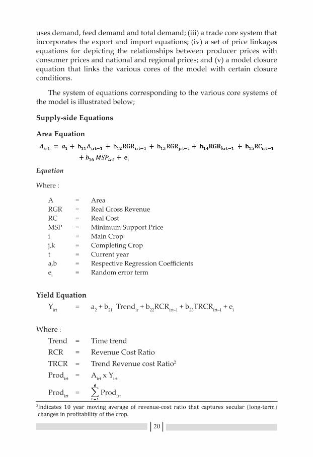
20

uses demand, feed demand and total demand; (iii) a trade core system that incorporates the export and import equations; (iv) a set of price linkages equations for depicting the relationships between producer prices with consumer prices and national and regional prices; and (v) a model closure equation that links the various cores of the model with certain closure conditions.

The system of equations corresponding to the various core systems of the model is illustrated below;

Supply-side Equations

Area Equation

Equation

Where :

A = AreaRGR = Real Gross RevenueRC = Real CostMSP = Minimum Support Pricei = Main Cropj,k = Completing Cropt = Current year a,b = Respective Regression Coefficientsei = Random error term

Yield EquationYirt = a2 + b21 Trendir + b22RCRirt–1 + b23TRCRirt–1 + ei

Where :

Trend = Time trendRCR = Revenue Cost RatioTRCR = Trend Revenue cost Ratio2

Prodirt = Airt x Yirt

Prodirt = Prodirt

2Indicates 10 year moving average of revenue-cost ratio that captures secular (long-term) changes in profitability of the crop.

21

Where :

Prodirt = Total production in region r

Prodrt = Total production in the country

Demand-side Equations

Food Demand

Where :

FD = Per capita food demand

PC = Real Consumer Price(Retail market price)

I = Real Income per capita

TFD = Total food demand

POP = Total population of the country

i = Main crop

j and k = Substitute crops

t = Current year

Feed DemandFeedit = a4 + b41 Feedit-1 + b42PCit + b43PCjt + ei

Total DemandTD it = TFDit + Feedit

Where :

Feed = Feed demandTD = Total demand

Ending StockESit = a5 + b51ESit-1 + b52MSPit +ei

Where :

ES = Ending stock

22

Change in stockSi = ESit + ESit-1

Export EquationEXPit = a6 + b61 ESit-1 +b62PRit+ei

Import EquationIMPit = a7 + b71 ESit-1 + b72PRit+ b73Tariff + ei

Where :

EXP = ExportPR = World price – consumer price ratioIMP = ImportTariff = Import tariff

Total Supply EquationTSit = Prodit+ Si

Price Linkage EquationsPPi = PCi – Margin3

i

PCR = a + bPC4N + ei

Where :

PP = Producer price (Farm harvest price)PC = Consumer price (Retail market price)Margin = Price spreadPCR = Regional consumer pricePCN = National representative cosumer price

Model ClosureTSit + Netradeit = TDit

Where :

TS = Total SupplyNetrade = Export - ImportTD = Total Demand

3Margin is estimated by subtracting regional producer price from regional consumer price till the base-year.4Market-clearing equilibrium price obtained through iterations beyond the base-year.

23

The above framework was specified for each of the three primary food commodities in the model. On the supply side, area, yield and production were modeled at the regional levels. For this, the country was divided into six regions, namely East, West, North, South, Hills and North-East and area and yield equations were fitted separately for each region under each crop.

A detailed commodity-wise picture on spatial and temporal dimensions of the model is outlined in Table 3.1.

Table 3.1: Cereal Outlook Model: Commodity, spatial and temporal dimensions

Primary crop Region Region detailsProduction

Wheat/ Rice/ Maize East Assam, Bihar, Odisha, West Bengal, Jharkhand

West Gujarat, Madhya Pradesh, Maharashtra, Rajasthan, Chhattisgarh

North Haryana, Punjab, Uttar Pradesh, Uttarakhand

South Andhra Pradesh, Karnataka, Kerala, Tamil Nadu

Hills Himachal Pradesh, Jammu and Kashmir

North-East Manipur, Meghalaya, Nagaland, Sikkim, Tripura, Arunachal Pradesh, Mizoram

DemandWheat/ Rice/ Maize All India All India

TradeWheat/ Rice/ Maize All India All India

StocksWheat/ Rice/ Maize All India All India

The estimates on production were obtained by multiplying the area and yield estimates for each of these regions, and the national production estimates were computed by aggregating these regional estimates. On the demand side, the country was treated as a single region and equations for food and feed demand were laid out for estimating the total demand for each crop. The demand arising from other uses such as industrial

24

requirements, seed, etc. are implicit in the food demand category in the balance sheet because of which a separate equation to represent them was not laid out. The food demand equations were initially specified at the per capita level. Their estimated values were subsequently multiplied with population figures to obtain the national estimates on total food demand. Similarly, the stocks and trade were also modeled at the national level. The trade equations does not include non-price factors such as quantitative restrictions or other variables to capture restrictions like minimum export prices, export/import ban etc. Each of the three primary crops was linked with the other through its competitive relationship on the supply side and substitutive relationship on the demand side. For instance, maize was treated as a competing crop for rice and vice versa and were accordingly inserted as exogenous variables in the area equations of respective crops. Similarly, both wheat and maize have been incorporated as substitute crops in the household demand equation for rice. In addition to the primary crops, other crops like chick pea, pigeon pea, rapeseed and mustard also appear in the model as auxiliary crops with varying relationships with the primary crops. The role of inputs in determining crop yield has been captured indirectly through the cost of cultivation variable that appears in the list of independent variables in the yield function. Sufficient care was taken to include the break-up of cost of cultivation on individual inputs such as human, bullock and animal labor, seed, fertilizers, irrigation, etc., so that variations in the cost of these inputs get reflected on the yield of the crop. All monetary values appearing in the Model were converted into real terms using Gross Domestic Product (GDP) deflator with the base-year 2004-05. The detailed model linkages and a list of endogenous and exogenous variables along with their technical parameters and elasticties are presented in Appendix 2.

The elasticities appearing in the Model were initially estimated outside the system using appropriate methodologies. For instance, the acreage elasticities were estimated by fitting acreage response models for each crop as well as for each region using time-series data. Similarly, the food demand elasticities were estimated by applying AIDS Framework on household consumption data. Other elasticities were estimated using simple regression procedures applied on time-series data. However, the final values of the elasticities were determined through calibrations. The technical parameters were obtained based on the calibrated elasticities and the actual data on respective variables within the model. The base data on all variables correspond to the period 1994-95 to 2010-11. The projections were carried out for the ensuing period between 2011-12 and 2025-26. In the baseline model, most of the exogenous variables (like RGR, RC, MSP, Margin, etc.) were assumed to grow with their real values remaining

25

constant beyond the base-year. However, projections on variables such as GDP, population and per capita income were obtained from reliable official sources (Appendix 3).

3.4. Simulations and Sensitivity Analysis

The functionality for undertaking sensitivity analysis and simulations has been incorporated in the Cereal Outlook Model. Simulations can be carried out by altering the baseline values of exogenous variables to reflect the changes in technological, policy and production possibility scenarios. Such exercises are helpful in analyzing the impact of various government policy interventions and alterations in technology frontiers on the major variables included in the Model. In the present context, two scenario analyses were attempted to see the response of the Model with respect to shocks in exogenous variables. These were (i) sustained 2 per cent real annual increase in MSP of wheat, rice and maize, over the base-line (ii) Sustained 2 per cent real annual increase in cost of cultivation (cost A1) of wheat, rice and maize, over the base-line. The results of the simulation exercises are discussed in the forthcoming section.

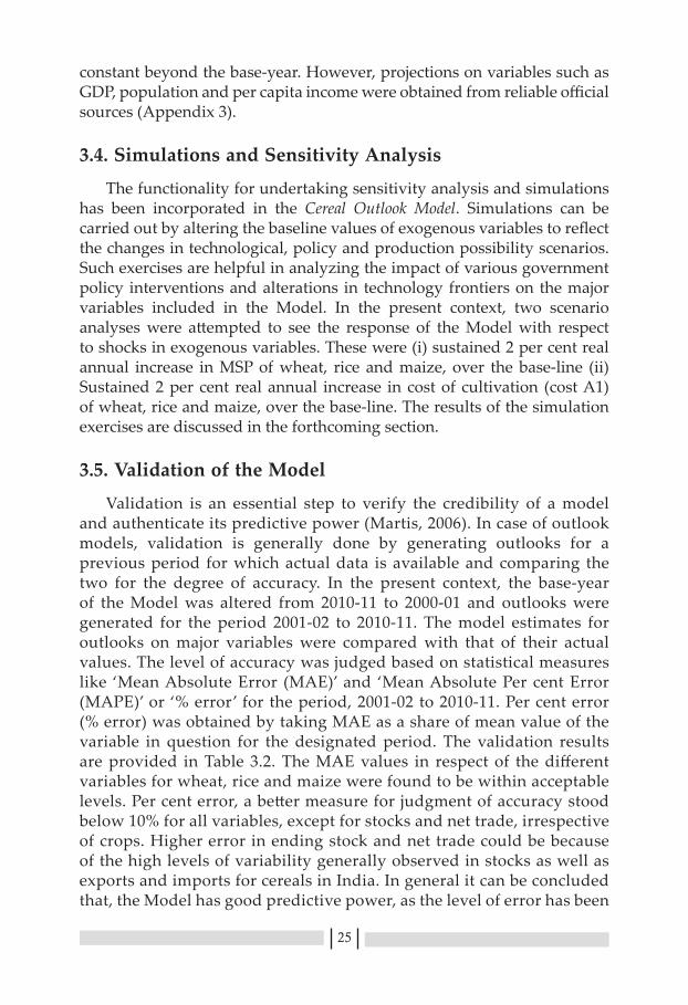
3.5. Validation of the Model

Validation is an essential step to verify the credibility of a model and authenticate its predictive power (Martis, 2006). In case of outlook models, validation is generally done by generating outlooks for a previous period for which actual data is available and comparing the two for the degree of accuracy. In the present context, the base-year of the Model was altered from 2010-11 to 2000-01 and outlooks were generated for the period 2001-02 to 2010-11. The model estimates for outlooks on major variables were compared with that of their actual values. The level of accuracy was judged based on statistical measures like ‘Mean Absolute Error (MAE)’ and ‘Mean Absolute Per cent Error (MAPE)’ or ‘% error’ for the period, 2001-02 to 2010-11. Per cent error (% error) was obtained by taking MAE as a share of mean value of the variable in question for the designated period. The validation results are provided in Table 3.2. The MAE values in respect of the different variables for wheat, rice and maize were found to be within acceptable levels. Per cent error, a better measure for judgment of accuracy stood below 10% for all variables, except for stocks and net trade, irrespective of crops. Higher error in ending stock and net trade could be because of the high levels of variability generally observed in stocks as well as exports and imports for cereals in India. In general it can be concluded that, the Model has good predictive power, as the level of error has been

26

found 5 per cent or lower for major variables like area, yield, production, consumption, etc. in case of wheat and rice and less than 10 per cent for maize.

Another indirect way of validating a model is to compare the results arising from it with that of other similar accepted models. In this case, the Cereal Outlook Model projections were compared with that of FAO/OECD model and FAPRI-CARD model (Appendix 5). The projections were found to be broadly comparable with one another.

Table 3.2. Results of validation of the Cereal Outlook Model(Area in Mha; Yield in T/ha; Production, Consumption, and Net trade in Mt)

Variable Wheat Rice Maize

MAE % error MAE % Error MAE % Error

Area 0.865 3.18 1.121 2.60 0.708 9.20

Yield 0.08 3.04 0.06 2.98 0.17 8.32

Production 3.678 4.91 4.532 5.04 1.629 10.10

Food and other use 2.354 3.25 3.900 4.52 0.609 7.80

Feed use 0.251 9.84 0.00 – 0.570 8.50

Total consumption 2.573 3.43 3.900 4.52 1.105 7.61

Ending stock 11.84 94.45 14.42 116.71 0.446 58.33

Net trade 2.896 126.35 2.017 48.70 1.337 83.62

Notes: ‘MAE’ denotes mean absolute deviation of projected values from actual for the period 2001-2010; ‘% Error’ denotes mean absolute per cent error.

3.6. Limitations of the ModelLike most other contemporary models, the Cereal Outlook Model also

has certain limitations which are elaborated here. The Model has been built under a linear framework, with all related equations specified in linear form. Consequently, all projections obtained from the Model would also follow linear paths, which is often not the case in reality. However, sufficient care is taken to ensure the most probable long-term trajectory of the concerned variables by calibrating the technical coefficients and validating the model for previous years for which data is available. Another limitation of the Model is that, some technical coefficients (particularly those corresponding to trade, stock and other minor variables) used in the model were obtained through calibration or from previous literature rather than through direct estimation. However, this is a standard procedure in modeling literature and would not affect the performance of the model beyond certain limits.

27

The values of the exogenous variables like per capita income, cost of cultivation, support prices, international prices, GDP deflator, etc. were either extrapolated based on logical assumptions or taken from other credible sources. The base-line projections are governed by the correctness of these assumptions to a considerable extent. Further, the linkages of the primary crops considered in the Model are limited only to a few immediately related crops. Broad linkages of the primary crops with other commodities outside the primary sector are also not covered in the present exercise. The Model also does not include elaborate linkages between MSP, procurement and distribution of the cereals considered. It was also assumed that, stocks of the grains are held only by the government and private stocks with the traders are negligible. Climatic variables such as rainfall, temperature, etc. are also kept aside due to constraints in estimating realistic technical parameters with respect to crop performance.

28

Main Results and Discussion

4.1. National and Regional Outlooks The base-line outlook estimates obtained from the Model for wheat, rice

and maize are presented in Tables 4.1 to 4.5. The results that correspond to the major endogenous variables viz., area, yield, production, food and feed consumption, stock as well as net trade are presented for the years 2011-12, 2016-17, 2020-21 and 2025-26 (Table 4.1). At all-India level, the area under wheat is projected to increase marginally from the base-year level of 29.04 Million hectare (Mha) to 30.11 Mha by the year 2025-26. This implies that the scope of area increase in wheat is limited and the production increase should come mainly from improvement in yield in future. The projections indicate that wheat yield in the country would increase modestly from the base-year value of 2.99 tonnes/hectare (t/ha) to 3.39 t/ha in a span of 15 years ahead. Consequently, the national production of wheat will increase by around 16 Million tonnes (Mt) during 2011-12 to 2025-26. The projections for wheat production are: 90.87 Mt by 2015-16, 95.59 Mt by 2020/21 and 102.08 Mt by 2025-26. The corresponding regional picture of future area, yield and production is also provided in Table 4.1. The highest share of wheat production would be from northern and western regions as in the past. Yield improvements are expected in all regions, but with the highest gains in eastern and northern regions. The demand for wheat is slated to increase due to increase in population and changes in dietary habits. At the national level, total demand for wheat is projected to grow from 81.60 Mt in 2010-11 to 102.0 Mt by 2025, the rate being slightly higher than growth in production. Accordingly, net trade of wheat would taper slightly from 0.67 Mt to 0.08 Mt during the period.

As in the case of wheat, area gains in rice would also be marginal, and within the range that had existed in the recent past. Projections from the Model indicate an area increase from 42.5 M ha in the base-year to 44.5 M ha by 2025-26 (Table 4.2). Yield gains in rice would be modest from 2.25 t/ha to 2.61 t/ha during this period. The total rice production is projected to rise from 95.7 Mt to 116.06 Mt. This growth would be shared across the regions with highest contribution from eastern and northern regions. The rice production in southern region is expected to stagnate mainly due to a decrease in area under the crop. In contrast, area under rice would increase

4

29

Table 4.1. Outlook for wheat in India: 2010-11 to 2025-26(Area in Mha; Yield in T/ha; Production, Consumption, Ending stock and Net trade in Mt)

Region Variable 2010-11 (Base-year)

2011-12 2016-17 2020-21 2025-26

All India

Area 29.04 29.20 29.37 29.68 30.11

Yield 2.99 2.96 3.09 3.22 3.39

Production 86.76 86.55 90.87 95.59 102.09

Food and other use 78.51 85.96 88.29 93.04 99.60

Feed use 3.10 2.69 2.51 2.48 2.41

Total consumption 81.61 88.65 90.80 95.52 102.01

Ending stock 21.41 19.17 18.91 18.91 18.91

Net trade 0.68 0.13 0.07 0.08 0.08East Area 2.56 2.59 2.61 2.63 2.64

Yield 2.02 2.09 2.21 2.31 2.42

Production 5.19 5.40 5.76 6.08 6.39West Area 9.51 9.50 9.53 9.68 9.81

Yield 2.24 2.28 2.39 2.52 2.63

Production 21.29 21.67 22.76 24.39 25.78North Area 16.04 16.16 16.28 16.50 16.69

Yield 3.68 3.60 3.74 3.93 4.09

Production 58.98 58.16 60.95 64.86 68.29South Area 0.27 0.28 0.29 0.30 0.30

Yield 1.10 1.03 1.12 1.22 1.30

Production 0.29 0.29 0.33 0.36 0.39Hills Area 0.65 0.67 0.65 0.65 0.65

Yield 1.53 1.51 1.63 1.76 1.87

Production 0.99 1.01 1.05 1.14 1.22North East

Area 0.01 0.01 0.01 0.01 0.01

Yield 1.50 1.59 1.58 1.57 1.56

Production 0.02 0.02 0.02 0.02 0.02

in eastern and northern regions with commensurate gains in yield. Slight gains in area and yield are also expected from the western region of the country.

30

Table 4.2. Outlook for rice in India: 2010-11 to 2025-26(Area in Mha; Yield in T/ha; Production, Consumption, Ending stock and Net trade in Mt)

Region Variable 2010-11 (Base-year)

2011-12 2016-17 2020-21 2025-26

All India Area 42.51 44.17 44.20 44.34 44.53

Yield 2.25 2.26 2.37 2.47 2.61

Production 95.74 100.01 104.82 109.60 116.07

Food and other use 90.21 96.55 100.81 105.72 112.03

Feed use 0.00 0.00 0.00 0.00 0.00

Total consumption 90.21 96.55 100.81 105.72 112.03

Ending stock 19.44 18.63 18.42 18.01 17.99

Net trade 2.77 4.27 4.04 4.03 4.04East Area 15.03 16.75 16.91 16.94 16.99

Yield 1.92 1.95 1.99 2.03 2.09

Production 28.82 32.64 33.63 34.39 35.46West Area 7.76 7.82 7.83 7.85 7.88

Yield 1.60 1.48 1.61 1.72 1.88

Production 12.39 11.58 12.58 13.50 14.78North Area 10.02 10.12 10.01 10.05 10.10

Yield 2.68 2.81 3.07 3.28 3.56

Production 26.85 28.43 30.69 32.94 35.99South Area 8.41 8.23 8.21 8.26 8.31

Yield 2.96 3.00 3.06 3.13 3.22

Production 24.92 24.67 25.10 25.81 26.73Hills Area 0.34 0.34 0.34 0.33 0.33

Yield 1.88 2.03 2.24 2.39 2.57

Production 0.64 0.68 0.75 0.80 0.85North- East

Area 0.94 0.91 0.91 0.91 0.91

Yield 2.25 2.20 2.29 2.37 2.48

Production 2.12 2.01 2.07 2.15 2.26

31

The total food demand for rice would increase from the base-year value of 90.20 Mt to 105.71 Mt by 2020-21 and further to 112.02 Mt by the year 2025-26. With sufficient balance of production over demand, the net trade in rice would remain positive and in the range of 4.0-4.20 Mt during 2011-12 to 2025-26. The area under maize is projected to increase at a higher rate than that of wheat and rice in per cent terms. The Model projects an increase in area from 8.61 M ha in the base-year to 9.14 M ha by the year 2025-26 (Table 4.3). The yield of maize is slated to increase perceivably

Table 4.3. Outlook for maize in India: 2010-11 to 2025-26

(Area in Mha; Yield in T/ha; Production, Consumption, Ending stock and Net trade in Mt)

Region Variable 2010-11 (Base-year)

2011-12 2016-17 2020-21 2025-26

All India Area 8.61 9.04 9.26 9.19 9.14Yield 2.54 2.62 2.73 2.86 2.98Production 21.84 23.72 25.26 26.31 27.20Food and other use

9.10 10.22 11.04 11.65 12.10

Feed use 9.00 10.43 11.51 11.85 12.24Total con-sumption

18.10 20.64 22.55 23.50 24.34

Ending stock 755 678 630 635 634

Net trade 3.48 3.16 2.72 2.81 2.86East Area 1.09 1.07 1.02 1.01 1.01

Yield 2.18 2.36 2.45 2.54 2.67Production 2.37 2.53 2.50 2.58 2.71

West Area 3.47 3.74 3.84 3.78 3.74Yield 1.94 2.01 2.01 2.10 2.22Production 6.71 7.52 7.73 7.94 8.31

North Area 0.93 0.93 0.93 0.92 0.91Yield 1.80 1.87 1.93 1.99 2.06Production 1.67 1.75 1.79 1.83 1.88

South Area 2.26 2.41 2.60 2.63 2.62Yield 4.17 4.26 4.44 4.58 4.79Production 9.43 10.27 11.55 12.05 12.52

Hills Area 0.61 0.62 0.61 0.61 0.61Yield 1.98 1.99 2.04 2.09 2.16Production 1.20 1.23 1.25 1.28 1.32

North-East

Area 0.27 0.26 0.26 0.25 0.25Yield 1.78 1.65 1.70 1.75 1.82Production 0.47 0.43 0.44 0.45 0.46

32

from 2.54 t/ha to 2.98 t/ha during this period. Both area and yield gains would result in the increase of maize production from 21.8 Mt to 27.19 Mt during the period under projection. Such gains in production would be appreciable for a marginal crop like maize, and indicate the future potential of this important low value staple crop. The regional outlook for maize suggests promising potential for this crop in eastern, western and southern regions. Significant yield improvements are expected in all these three regions, though northern and hills are not far behind. However, maize production is projected to dip in north-eastern region with loss in area and stagnation in yield. On the demand side, projections have shown that use of maize both as food and feed will increase considerably. While the food demand for maize would increase from 9.10 Mt to 12.23 Mt, the feed demand would rise more or less at the same rate from 9.0 Mt to 10.6 Mt during the period of projection. The higher growth in demand over production would result in net trade to dip from 3.47 Mt to 2.86 Mt over the next fifteen years.

The market clearing prices for rice, wheat and maize at which the supply-demand equilibriums were arrived at are presented in Appendix 4. The equilibrium outlook estimates presented above were essentially the ones corresponding the marketing clearing prices as explained previously.

4.2. Simulation ResultsAs outlined in the methodology section, two separate simulations were

carried out using Cereal Outlook Model and the results are presented in Table 6 and 7. The first one corresponds to a sustained 2 per cent real annual increase in MSP of wheat, rice and maize during the projection period. The results are expressed in terms of percent changes over base-line. It was observed that increase in MSP, an exogenous policy variable, resulted in increase of area, production, consumption as well as net trade in all three commodities. The simulations indicate that, per cent increase in area under cultivation for wheat, rice and maize respectively would be 0.09 per cent, 0.15 per cent and 0.09 per cent respectively in the immediate next period after the base-year (Table 4.4). The area would further increase consistently over the years to reach at 1.68 per cent, 2.50 per cent and 2.36 per cent by the year 2025-26 over the base-year. The increase in area under cultivation would resultantly cause production to rise over the years with subsequent positive effects on consumption as well. However, the magnitude of consumption rise would be a little less than production allowing the excess production to get exported thereby recording increase in net trade. In general, rice and maize were found to be better responsive to changes in MSP than wheat in terms of corresponding changes in area, production and consumption. However, this was converse in case of net trade, with

33

higher per cent increase in net trade of wheat as against that of rice and maize. Another notable finding was that, market clearing prices of all three crops decreased as a result of increase in MSP and consequent increase in area and production. This shows that, excessive dependence on MSP as a policy variable to improve farmers’ welfare may have unintended negative implications. Therefore, government interventions should based on proper evaluation of all dimensions of its effects on the economy.

Table 4.4. Effects of sustained 2% annual increase (in real terms) in MSP of wheat, rice and maize

(% change over the base-line)

Variable Crop 2011-12 2016-17 2020-21 2025-26Area Wheat 0.09 0.61 1.07 1.68

Rice 0.15 0.92 1.59 2.50

Maize 0.09 0.82 1.47 2.36

Production Wheat 0.09 0.43 0.70 1.01Rice 0.16 0.74 1.22 1.83

Maize 0.09 0.71 1.26 1.98

Total consumption

Wheat 0.06 0.40 0.66 0.97Rice 0.14 0.70 1.16 1.75

Maize 0.08 0.69 1.22 1.91Net trade Wheat 1.14 11.07 18.03 26.03

Rice 0.36 1.52 2.49 3.73

Maize 0.07 0.77 1.48 2.50

Market clearing price

Wheat -0.55 -2.84 -4.67 -6.75Rice -0.95 -4.28 -6.84 -9.87

Maize -0.23 -1.86 -3.46 -5.77

Simulation results from the Model indicate that sustained increase in cost of cultivation at the rate of 2 per cent per annum would result in decline of area, production, consumption and net trade in all three commodities. Intuitively, as cost of cultivation increases, farmers would tend to reduce their area under crops. In case of wheat, the reduction of area would be to the tune of 0.08 per cent from the base-line by the year 2025-26 (Table 4.5). Area reduction in rice would be at 0.02 per cent in relation to baseline, where as there would be negligible effects on maize area. Lower area under cultivation would therein result lower production and so are the indications from the simulations in the present context. The corresponding decline in production of wheat, rice and maize would be at 0.21 per cent, 0.13 per cent and 0.13 per cent respectively by the year 2025-26. The relatively higher magnitude in decline of production is due to reduction in yield of crops as well as a result of increase in cost of cultivation. Equivalent squeeze in

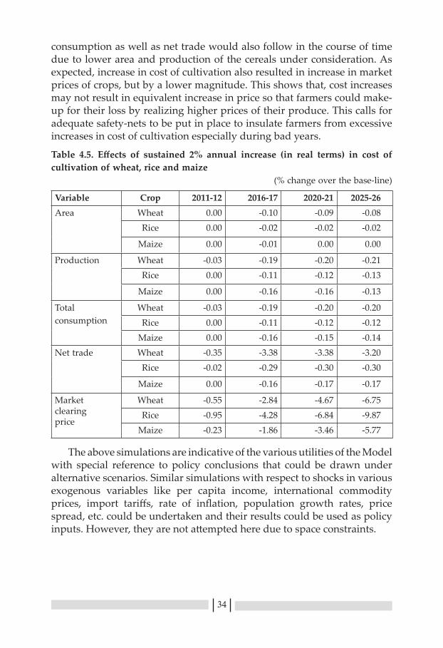
34

consumption as well as net trade would also follow in the course of time due to lower area and production of the cereals under consideration. As expected, increase in cost of cultivation also resulted in increase in market prices of crops, but by a lower magnitude. This shows that, cost increases may not result in equivalent increase in price so that farmers could make-up for their loss by realizing higher prices of their produce. This calls for adequate safety-nets to be put in place to insulate farmers from excessive increases in cost of cultivation especially during bad years.

Table 4.5. Effects of sustained 2% annual increase (in real terms) in cost of cultivation of wheat, rice and maize (% change over the base-line)

Variable Crop 2011-12 2016-17 2020-21 2025-26Area Wheat 0.00 -0.10 -0.09 -0.08

Rice 0.00 -0.02 -0.02 -0.02

Maize 0.00 -0.01 0.00 0.00

Production Wheat -0.03 -0.19 -0.20 -0.21Rice 0.00 -0.11 -0.12 -0.13

Maize 0.00 -0.16 -0.16 -0.13

Total consumption

Wheat -0.03 -0.19 -0.20 -0.20Rice 0.00 -0.11 -0.12 -0.12

Maize 0.00 -0.16 -0.15 -0.14Net trade Wheat -0.35 -3.38 -3.38 -3.20

Rice -0.02 -0.29 -0.30 -0.30

Maize 0.00 -0.16 -0.17 -0.17

Market clearing price

Wheat -0.55 -2.84 -4.67 -6.75Rice -0.95 -4.28 -6.84 -9.87

Maize -0.23 -1.86 -3.46 -5.77

The above simulations are indicative of the various utilities of the Model with special reference to policy conclusions that could be drawn under alternative scenarios. Similar simulations with respect to shocks in various exogenous variables like per capita income, international commodity prices, import tariffs, rate of inflation, population growth rates, price spread, etc. could be undertaken and their results could be used as policy inputs. However, they are not attempted here due to space constraints.

35

Conclusions and Policy Implications

A far sighted food policy is essential to facilitate efficient functioning of food production and management systems, especially for a country like India where household level food security still remains elusive. In this context, reliable mechanisms for generating outlooks on key variables such as demand, supply, trade, prices, etc. of important food commodities forms an essential basis for planning. This Paper explores the theoretical underpinnings as well as practical applications of Cereal Outlook Model, a dynamic, partial equilibrium model, developed by the authors with the specific purpose of generating future outlooks on major cereals in India. Demand-and-supply-side outlook on key variables such as area, yield, production, consumption and net trade of wheat, rice and maize have been attempted with projections extending up to 2025-26. On the supply side, area, yield and production were modeled at the regional levels. For this, the country was divided into six regions, namely East, West, North, South, Hills and North-East and area and yield equations were fitted separately for each region under each crop. The estimates on production were obtained from the estimates on area and yield for each of these regions, and the national production estimates were computed by aggregating these regional estimates. On the demand side, the country was treated as a single region and equations for food and feed demand were laid out for estimating the total demand for each crop. The food demand equations were initially specified at the per capita level. Their estimated values were subsequently adjusted for population to obtain the national estimates on total food demand. Similarly, the stocks and trade were also modeled at the national level. In the modeling framework, each of the three primary crops was linked with the other auxiliary crops such as chick pea, pigeon pea, rapeseed and mustard, etc. through their competitive relationship on the supply side and substitutive relationship on the demand side. The technical coefficients appearing in the model were initially obtained separately using appropriate demand and supply estimation techniques. However, the final values of the elasticities were determined through model calibrations. The base data on all variables correspond to the period 1994-95 to 2010-11, for which the elaborate demand, supply and trade core systems were laid out. Projections for future years were carried out

5

36

based on a recursive dynamic iterative algorithm that satisfy the closure condition that total demand of a particular commodity in an year equals its total supply, after adequately accounting for the respective trade and stock balances. Accordingly, the projections cover the period 2011-12 to 2025-26 with the base-year of projections being 2010-11.

The model results indicate fast growing trends in demand and supply of the three cereals considered. At all-India level, the area under wheat is projected to increase marginally from the base-year level of 29.04 Million hectare (Mha) to 30.11 Mha by the year 2025-26. This implies that the scope of area increase in wheat is limited and the production increase should come mainly from improvement in yield in future. The yield projections indicate that wheat yield in the country would increase modestly from the base-year value of 2.99 tonnes/hectare (t/ha) to 3.39 t/ha in a span of 15 years ahead. Consequently, the national production of wheat will increase by around 16 Million tonnes (Mt) during 2011-12 to 2025-26 with the respective production projections being 90.87 Mt for 2015-16, 95.59 Mt for 2020/21 and 102.08 Mt for 2025-26.As in the case of wheat, area gains in rice would also be marginal, and within the range that has existed in the recent past. Projections from the Model indicate an area increase from 42.5 M ha in the base-year to 44.5 M ha by 2025-26. Yield gains in rice would be modest from 2.25 t/ha to 2.61 t/ha during this period. Consequently, the total rice production is projected to rise from 95.7 Mt to 116.06 Mt. The area under maize is projected to increase at a higher rate than that of wheat and rice in relative terms. The Model projects an increase in area from 8.61 M ha in the base-year to 9.14 M ha by the year 2025-26 for maize. The yield of maize is slated to increase perceivably from 2.54 t/ha to 2.98 t/ha during this period. Both area and yield gains would result in the increase of maize production from 21.8 Mt to 27.19 Mt between the base-year and terminal year of projections. Such gains in production would be appreciable for a marginal crop like maize, and indicate the future potential of this important low value staple crop.

In nutshell, the outlooks on rice, wheat and maize obtained from the Model indicates that, though demand for these crops would increase considerably as a result of growing per capita income, population and urbanization, supply would keep pace owing to the emergence of new areas contributing towards incremental production. Regional supply projections indicate strong potential in the eastern region of the country with promising outlooks on area and yield for all three crops in this region. This augurs well with the recent initiatives of the government of India in extending green revolution to eastern India with substantial allocations for improving input delivery systems, market development and infrastructure creation. The prominence of northern region would continue particularly

37

for wheat and rice. The southern and western regions would maintain their status quo, but production projections indicate a general tendency of stagnation in these two regions. The contribution of hill and north-eastern regions would remain negligible as in the past. Consequent to the considerable supply response projected against the growing demand, the net trade of all three commodities would remain positive, though some signs of tapering off in net trade are expected in case of wheat and maize. Accordingly, no serious supply deficits are to be anticipated in case of the three cereals considered at least for the next one and a half decades in the country.

The functionality of the Model to undertake simulations under alternative technology and policy scenarios was also demonstrated in the Paper. The simulation results corresponding to two scenarios of sustained increase in MSP and cost of cultivation of the three crops were consistent with intuitive hypotheses. It was observed that increase in MSP, an exogenous policy variable, resulted in increase of area, production, consumption as well as net trade in all three commodities. Similarly, the simulations with respect to sustained increase in cost of cultivation resulted in decline of area, production, consumption and net trade in all the three commodities. In nutshell, the paper throws light on a time tested, but relatively less explored approach to derive future outlooks on important staple crops that could have significant say in the country’s food security in times to come.

38

References

Alston J.M., Norton G.W. and Pardey P.G. (1998). Science under Scarcity. CAB International.

Bhalla, G.S., Hazell, Peter and Kerr, John (1999).Prospects for India’s cereal supply and demand to 2020. Food, Agriculture and the Environment Discussion Paper 29, Washington DC: International Food Policy Research Institute.

Binfield, J., Donnellan, T. and McQuinn, K. (2000). The econometric modeling of agricultural policy: An Irish example, Paper submitted to Agricultural Economics Society, Manchester: Manchester University.

Chand, Ramesh (2007). Demand for food grains. Economic and Political Weekly, 42(52), 10-13.

Chand, Ramesh (2009). Demand for food grains during 11th plan and towards 2020. Policy Brief No. 28, New Delhi: National Centre for Agricultural Economics and Policy Research.

Conforti, Piero (2001). The common agricultural policy in main partial equilibrium models. Working Paper No. 7, Rome: The National Institute of Agricultural Economics.

Dastagiri, M.B., (2004). Demand for Livestock Products in India: Current Status and Projections for 2020. Policy Paper No. 21,New Delhi: National Centre for Agricultural Economics and Policy Research.

Rajaraman, Indira and Datta, Arindam (2003).Univariate forecasting of state-level agricultural production, Economic and Political Weekly, 38(18): 1800-1803.

Devadoss, S.D., Helmar, M.D. and Meyers, W.H. (1989). FAPRI trade model for the wheat sector: specification, estimation and validation. Technical Report 90, Center for Agricultural and Rural Development, Ames: Iowa State University.

Devadoss S. D., Westhoff P. C., Helmar M. D., Grundmeier E., Skold K., Meyers W. H and Johnson S. R. (1993). The FAPRI Modelling System: A Documentation Summary. Taylor C. R., Reichelderfer K.H. and Johnson S.R. (eds.) Agricultural Sector Models for United States: Descriptions and Selected Policy Applications, Ames: Iowa State University Press.

39

ERS (2013).Website of Economic Research Service of the USDA at www.ers.usda.gov accessed in July, 2013.

FAPRI (2004).Documentation of FAPRI modeling system. FAPRI-UMC Report 12-04, Columbia MO: Food and Agricultural Policy Research Institute.

Fuller,Frank(1997). Policy and Projection Model for the Meat Sector in the People’s Republic of China, Technical Report 97-TR 36, Centre for Agricultural and Rural Development, Ames: Iowa State University.

Fuller, Frank, Wailes, Eric, J. and Djunaidi, Hariyanto(2004).Revised Arkansas Global Rice Model, Staff General Research Papers11790, Department of Economics, Ames: Iowa State University.

GoI (2001).Population Projections for India and States: 1996-2016. New Delhi: Registrar General, Government of India.

Gujarati, Damodar (2003). Basic Econometrics, Fourth Edition, New Delhi: Tata McGraw-Hill Publishing Company Limited.

Kannan, R. and Chakrabarty, T.K. (1983). Demand projections for selected food items in India, 1985-86 to 2000-01, Economic and Political Weekly,18 (52).

Kumar, Ganesh, A. (1992). Falling agricultural investments and its consequences, Economic and Political Weekly, 27(42), 2307-2312.

Kumar, Praduman (1998). Food Demand and Supply Projections for India, Agricultural Economics Policy Paper No. 98-01. New Delhi: Indian Agricultural Research Institute.

Kumar, Praduman, Joshi, P.K. and Birthal, P. S. (2009). Demand projections for foodgrains in India. Agricultural Economics Research Review, 22(2), 237-243.

Kumar, Praduman, Shinoj P., Raju, S.S., Kumar, Anjani, Karl M. Rich and Msangi, Siwa. (2010). Factor demand, output supply elasticities and supply projections for major crops in India. Agricultural Economics Research Review, 23 (1), 1-14.

Lampe, Martin von (2005). The World Agricultural Simulation System (WATSIM): an overview. Discussion Paper No. 98-01, Bonn: University of Bonn.

Martis, M.S. (2006). Validation of simulation based models: A theoretical outlook. The Electronic Journal of Business Research Methods, 4(1), 39-46.

40

McCalla, Alex, F and Revoredo, Cesar, L. (2001). Prospects for global food security: a critical appraisal of past projections and predictions, Washington, DC: International Food Policy Research Institute.

Meyer, F.H., Kirsten, J.F. and Poonyth, D. (2003). Modeling the market outlook and policy alternatives for the wheat sector in South Africa, Contributed paper presented at the 41st Annual Conference of the Agricultural Economic Association of South Africa (AEASA), Pretoria, South Africa.

Mittal, Surabhi (2006). Structural Shift in Demand for Food: India’s Prospects in 2020. Working Paper No. 184, New Delhi: Indian Council for Research on International Economic Relations.

Mythili, G. (2006). Supply response of Indian farmers: Pre-and-post-reforms. Working Paper 2006-009, Mumbai: Indira Gandhi Institute of Development Research.

Narain P., Pandey, R.K. and Sarup, S. (1985). On food grains production projections, Agricultural Situation in India, 40 (5): 353-358.

NCAER (2013). Agricultural Outlook and Situation Analysis Reports, First semi-annual medium-term agricultural outlook report, New Delhi: National Council for Applied Economics Research.

OECD/FAO (2011). OECD-FAO Agricultural Outlook 2011-2020. OECD Publishing and FAO. Retrieved from http://dx.doi.org/10.1787/agr_outlook-2011-en.

Parikh, Kirit, S., Narayana, N.S.S, Panda, Manoj and Kumar, Ganesh, A. (1995). Strategies for agricultural liberalization: Consequences for growth, welfare and distribution. Economic and Political Weekly, 30(39), A-90-92.

Parikh, Kirit, S., Kumar, Ganesh, A. and Darbha, Gangadhar (2003). Growth and welfare consequences of rise in MSP. Economic and Political Weekly, 38(9), 891-895.

Paroda, R.S. and Kumar, P. (2000). Food production and demand in South Asia, Agricultural Economics Research Review, 3 (1): 1-24.

Radhakrishna, R. and Ravi.C. (1994). Food demand in India: Emerging trends and perspectives. Hyderabad: Centre for Economic and Social Studies. Mimeo.

Rosegrant, Mark, W. and the IMPACT Development Team (2012). International Model for Policy Analysis of Agricultural Commodities

41

and Trade (IMPACT): model description. Washington DC: International Food Policy Research Institute.

Stout, James and Abler, David(2004). ERS/PENN State Trade Model Documentation, The Pennsylvania State University, accessed at http://trade.aers.psu.edu/pdf/ERS Penn State Model Documentation.pdf.

Tongeren, F.V., Meijl, H.V. and Surry, Y. (2001). Global models applied to agricultural and trade policies: a review and assessment, Agricultural Economics, 26 (2), 149-172.

Wailes, Eric J.(2004). Review of existing global rice market models, Session 17: Rice supply and demand, Proceedings of the World Rice Research conference, Tsukuba, Japan, 4-7 November, 2004.

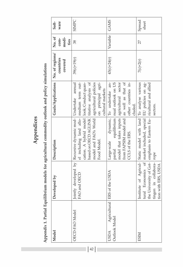
42

App

endi

ces

App

endi

x 1.

Par

tial E

quili

briu

m m

odel

s fo

r ag

ricu

ltura

l com

mod

ity o

utlo

ok a

nd p

olic

y si

mul

atio

ns

Mod

elD

evel

oped

by

Des

crip

tion

Goa

ls/A

pplic

atio

nsN

o. o

f re

gion

s/co

untr

ies

co

vere

d

No.

of

com

-m

odi-

ties

Soft-

war

e

OEC

D-F

AO

Mod

elJo

intly

dev

elop

ed b

y FA

O a

nd O

ECD

Recu

rsiv

e dy

nam

ic m

od-

el

incl

udin

g la

nd

allo

-ca

tion.

A h

ybri

d m

odel

ba

sed

on O

ECD

AG

LIN

K

mod

el a

nd F

AO

’s W

orld

Fo

od M

odel

.

Und

erta

ke

annu

al

med

ium

ter

m o

ut-

look

; Con

duct

qua

n-tit

ativ

e an

alys

is

of

agri

cultu

ral

polic

ies

on

prin

cipa

l ag

ri-

cultu

ral m

arke

ts

39(c

)+19

(r)

38SI

MPC

USD

A

Agr

icul

tura

l O

utlo

ok M

odel

ERS

of th

e U

SDA

Larg

e-sc

ale

dyna

mic

, pa

rtia

l eq

uilib

rium

m

odel

tha

t ta

kes

inpu

ts

from

FA

PSIM

mod

el a

nd

CC

LS o

f the

ERS

.

To

unde

rtak

e an

-nu

al o

utlo

ok o

n U

S ag

ricu

ltura

l se

ctor

as

wel

l as

tha

t of

ot

her

coun

trie

s in

-cl

uded

.

43(c

)+24

(r)

Vari

able

GA

MS

ESIM

Inst

itute

of

A

gric

ul-

tura

l Ec

onom

ics

of

the

Uni

vers

ity o

f Got

-tin

gen

in

colla

bora

-tio

n w

ith E

RS, U

SDA

Stat

ic m

odel

with

lan

d m

arke

t in

clud

ed, s

peci

al

emph

asis

to

East

ern

Eu-

rope

To a

naly

se v

ario

us

EU p

olic

ies

on a

g-ri

cultu

ral a

nd a

llied

se

ctor

s.

7(c)

+2(r

) 27

Spre

ad

shee

t

43

Mod

elD

evel

oped

by

Des

crip

tion

Goa

ls/A

pplic

atio

nsN

o. o

f re

gion

s/co

untr

ies

co

vere

d

No.

of

com

-m

odi-

ties

Soft-

war

e

FAPR

I-CA

RD M

odel

FA

PRI

and

CA

RD,

Iow

a St

ate

Uni

vers

ityEc

onom

etri

c re

curs

ive

dyna

mic

mod

el,

with

a

spec

ial e

mph

asis

on

US

Ann

ual

shor

t, m

e-di

um a

nd lo

ng te

rm

proj

ectio

ns;

Qua

n-tit

ativ

e ev

alua

tion

of

(inte

r)

natio

nal

agri

cultu

ral

polic

ies

that

affe

ct U

S an

d w

orld

agr

icul

ture

.

29(c

+r)

24SA

S-A

RE-

MO

S,

Spre

ad

shee

t

WA

TSIM

Inst

itute

of

A

gric

ul-

tura

l Po

licy,

Bo

nn

Uni

vers

ity, G

erm

any

Stat

ic m

odel

M

ediu

m a

nd l

ong-

term

out

look

; Pol

icy

anal

ysis

of

vari

ous

shift

fac

tors

inc

ome

chan

ges,

pro

duct

iv-

ity

grow

th,

trad

e lib

eral

izat

ion,

etc

.

4(c

)+ 1

0(r)

29Fo

rtra

n,

GA

MS

IMPA

CT

Mod

elIF

PRI,

Was

hing

ton,

D

.C.

Dyn

amic

m

odel

w

ith

spec

ial

com

pone

nt

on

land

and

wat

er d

ynam

-ic

s ac

ross

reg

ions

.

Polic

y an

alys

is

on

glob

al

food

de

-m

and,

sup

ply,

trad

e an

d pr

ices

and

thei

r lin

kage

s w

ith v

ari-

ous

bioe

nerg

y,

cli-

mat

e ch

ange

an

d di

vers

ifica

tion

sce-

nari

os.

115(

c)+

126(

r)44

GA

MS

Sour

ce: C

onfo

rti (

2001

); FA

PRI (

2004

); La

mpe

(200

5); O

ECD

/FA

O (2

011)

; Ros

egra

nt et

al (

2012

); To

nger

en et

al (

2001

).

44

Appendix 2

Cereal Outlook Model: Specifications

Region Dependent variable

Explanatory variable Parameter Elasticity

Crop: Wheat

Area equations

East Wheat area InterceptWheat lagged areaWheat lagged real gross returnsChickpea lagged real gross returnsRapeseed & mustard lagged real gross returnsWheat lagged real costWheat real minimum support price

2291.570.1340.009

-0.005-0.006-0.0130.025

0.1350.054

-0.031-0.033-0.0830.075

West Wheat area InterceptWheat lagged areaWheat lagged real gross returnsChickpea lagged real gross returnsRapeseed & mustard lagged real gross returnsWheat lagged real costWheat real minimum support price

5524.630.3310.031

-0.012-0.003-0.0210.034

0.3160.087

-0.026-0.016-0.1120.094

North Wheat area InterceptWheat lagged areaWheat lagged real gross returnsChickpea lagged real gross returnsRapeseed & mustard lagged real gross returnsWheat lagged real costWheat real minimum support price

7121.680.5570.029

-0.024-0.014-0.0350.097

0.5530.048

-0.027-0.019-0.0610.048

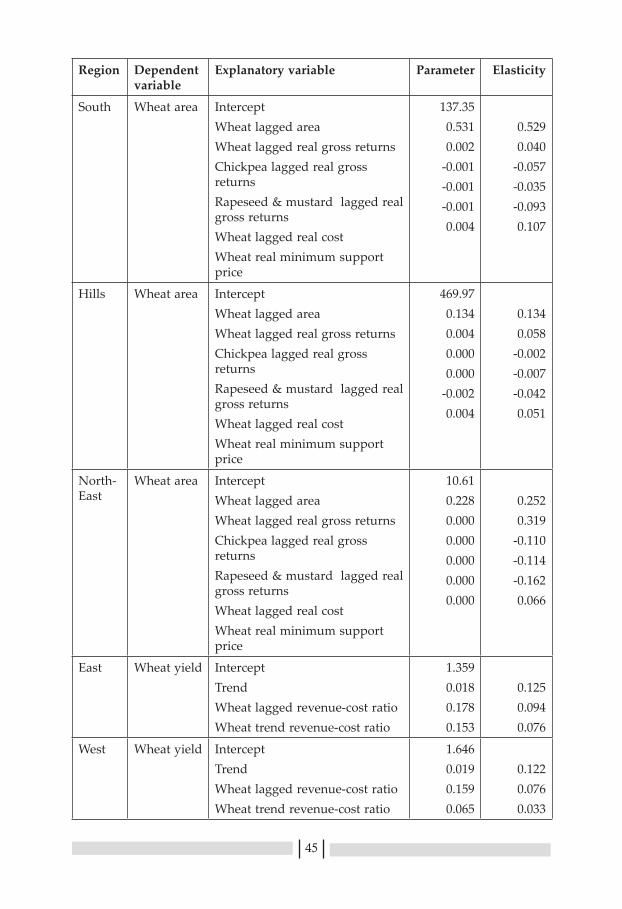
45

Region Dependent variable

Explanatory variable Parameter Elasticity

South Wheat area InterceptWheat lagged areaWheat lagged real gross returnsChickpea lagged real gross returnsRapeseed & mustard lagged real gross returnsWheat lagged real costWheat real minimum support price

137.350.5310.002

-0.001-0.001-0.0010.004

0.5290.040

-0.057-0.035-0.0930.107

Hills Wheat area InterceptWheat lagged areaWheat lagged real gross returnsChickpea lagged real gross returnsRapeseed & mustard lagged real gross returnsWheat lagged real costWheat real minimum support price

469.970.1340.0040.0000.000

-0.0020.004

0.1340.058

-0.002-0.007-0.0420.051

North-East

Wheat area InterceptWheat lagged areaWheat lagged real gross returnsChickpea lagged real gross returnsRapeseed & mustard lagged real gross returnsWheat lagged real costWheat real minimum support price

10.610.2280.0000.0000.0000.0000.000

0.2520.319

-0.110-0.114-0.1620.066

East Wheat yield InterceptTrendWheat lagged revenue-cost ratioWheat trend revenue-cost ratio

1.3590.0180.1780.153

0.1250.0940.076

West Wheat yield InterceptTrendWheat lagged revenue-cost ratioWheat trend revenue-cost ratio

1.6460.0190.1590.065

0.1220.0760.033

46

Region Dependent variable

Explanatory variable Parameter Elasticity

North Wheat yield InterceptTrendWheat lagged revenue-cost ratioWheat trend revenue-cost ratio

2.5570.0300.2200.193

0.1200.0620.052

South Wheat yield InterceptTrendWheat lagged revenue-cost ratioWheat trend revenue-cost ratio

0.5150.0160.1780.106

0.2520.0810.046

Hills Wheat yield InterceptTrendWheat lagged revenue-cost ratioWheat trend revenue-cost ratio

0.9600.0230.1170.049

0.2170.0650.032

North-East

Wheat yield InterceptTrendWheat lagged revenue-cost ratioWheat trend revenue-cost ratio

1.444-0.0030.1130.064

-0.0250.0490.025

All India

Wheat household per capita food demand

InterceptWheat lagged per capita food demandWheat real consumer priceRice real consumer priceMaize real consumer priceReal per capita income

77.02-0.057-1.9910.2710.3210.000

-0.056-0.2600.0620.0380.036

All India

Wheat total feed demand

InterceptWheat lagged feed demandWheat real consumer priceMaize real consumer price

3173.000.013

-0.1200.045

0.013-0.4010.138

All India

Wheat ending stock

InterceptWheat lagged ending stock Wheat real minimum support price

10083.930.1060.113

0.0930.072

All India

Wheat export

InterceptWheat lagged ending stockWheat world price-consumer price ratio

354.230.000

130.2530.0000.277

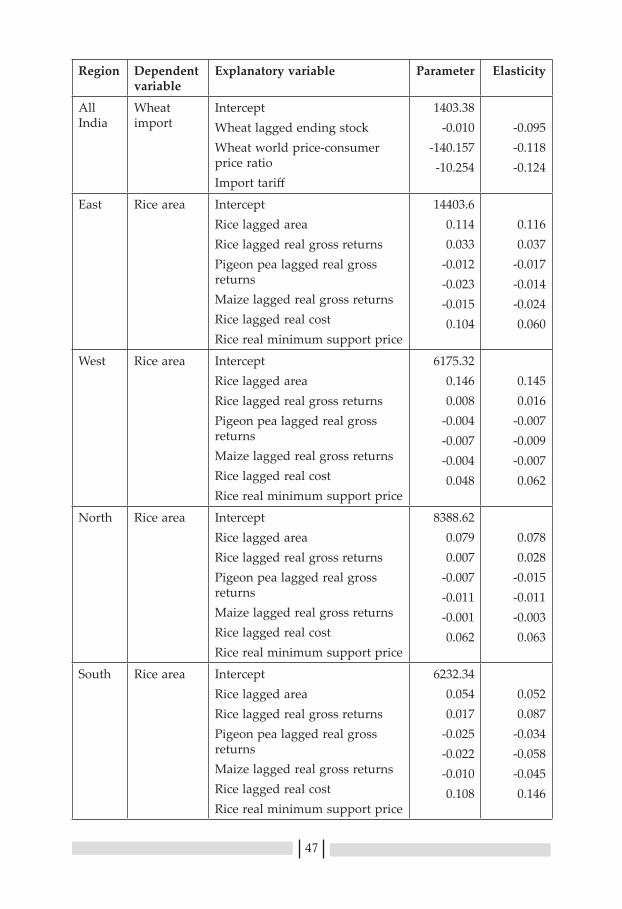
47

Region Dependent variable

Explanatory variable Parameter Elasticity

All India

Wheat import

InterceptWheat lagged ending stockWheat world price-consumer price ratioImport tariff

1403.38-0.010

-140.157-10.254

-0.095-0.118-0.124

East Rice area InterceptRice lagged areaRice lagged real gross returnsPigeon pea lagged real gross returnsMaize lagged real gross returnsRice lagged real costRice real minimum support price

14403.60.1140.033

-0.012-0.023-0.0150.104

0.1160.037

-0.017-0.014-0.0240.060

West Rice area InterceptRice lagged areaRice lagged real gross returnsPigeon pea lagged real gross returnsMaize lagged real gross returnsRice lagged real costRice real minimum support price

6175.320.1460.008

-0.004-0.007-0.0040.048

0.1450.016

-0.007-0.009-0.0070.062

North Rice area InterceptRice lagged areaRice lagged real gross returnsPigeon pea lagged real gross returnsMaize lagged real gross returnsRice lagged real costRice real minimum support price

8388.620.0790.007

-0.007-0.011-0.0010.062

0.0780.028

-0.015-0.011-0.0030.063

South Rice area InterceptRice lagged areaRice lagged real gross returnsPigeon pea lagged real gross returnsMaize lagged real gross returnsRice lagged real costRice real minimum support price

6232.340.0540.017

-0.025-0.022-0.0100.108

0.0520.087

-0.034-0.058-0.0450.146

48

Region Dependent variable

Explanatory variable Parameter Elasticity

Hills Rice area InterceptRice lagged areaRice lagged real gross returnsPigeon pea lagged real gross returnsMaize lagged real gross returnsRice lagged real costRice real minimum support price

282.970.2100.000

-0.0010.000

-0.0010.002

0.209-0.035-0.024-0.013-0.0410.065

North-East

Rice area InterceptRice lagged areaRice lagged real gross returnsPigeon pea lagged real gross returnsMaize lagged real gross returnsRice lagged real costRice real minimum support price

738.160.1480.001

-0.001-0.002-0.0030.007

0.1460.029

-0.015-0.018-0.0600.080

East Rice yield InterceptTrendRice lagged revenue-cost ratioRice Trend revenue cost ratio

1.540.0100.1400.084

0.0710.0560.035

West Rice yield InterceptTrendRice lagged revenue-cost ratioRice Trend revenue-cost ratio

0.850.0260.0850.074

0.2550.0730.057

North Rice yield InterceptTrendRice lagged revenue-cost ratioRice Trend revenue-cost ratio

1.730.0490.1490.078

0.2470.0660.034

South Rice yield InterceptTrendRice lagged revenue-cost ratioRice Trend revenue-cost ratio

2.480.0160.1100.086

0.0740.0420.035

Hills Rice yield InterceptTrendRice lagged revenue-cost ratioRice Trend revenue-cost ratio

1.430.0230.0980.071

0.1580.0580.040

49

Region Dependent variable

Explanatory variable Parameter Elasticity

North-East

Rice yield InterceptTrendRice lagged revenue-cost ratioRice Trend revenue-cost ratio

1.520.0210.0830.049

0.1400.0560.036

All India

Rice household per capita food demand

InterceptRice lagged per capita food demandRice real consumer priceWheat real consumer priceMaize real consumer priceReal per capita income

80.29-0.031-1.2060.7090.5620.000

-0.031-0.2300.0780.0570.026

All India

Rice total feed demand

InterceptRice lagged feed demandRice real consumer priceMaize real consumer price

0.0000.0000.0000.000

0.0000.0000.0000.000

All India

Rice ending stock

InterceptLagged ending stock Rice real minimum support price

8693.360.2380.030

0.2110.0265

All India

Rice export InterceptRice lagged ending stockRice world price-consumer price ratio

2082.800.004

984.9150.0130.426

All India

Rice import InterceptRice lagged ending stockRice world price-consumer price ratioImport Tariff

0.0680.0000.023

-0.056

0.0620.031

-0.105

East Maize area InterceptMaize lagged areaMaize lagged real gross returnsPigeon pea lagged real gross returnsRice lagged real gross returnsMaize lagged real costMaize real minimum support price

239.890.6160.010

-0.001-0.001-0.0010.015

0.5960.137

-0.023-0.016-0.0190.087

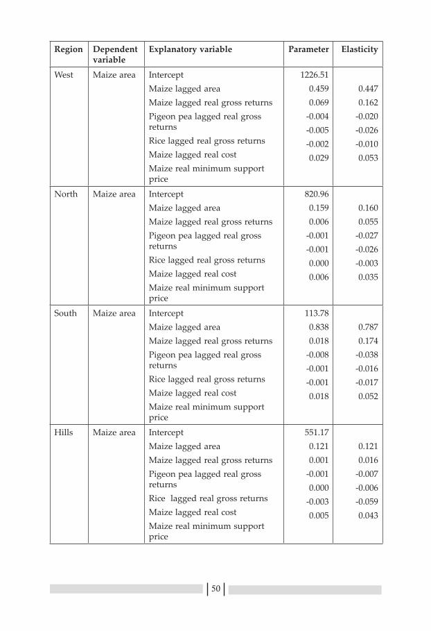
50

Region Dependent variable

Explanatory variable Parameter Elasticity

West Maize area InterceptMaize lagged areaMaize lagged real gross returnsPigeon pea lagged real gross returnsRice lagged real gross returnsMaize lagged real costMaize real minimum support price

1226.510.4590.069

-0.004-0.005-0.0020.029

0.4470.162

-0.020-0.026-0.0100.053

North Maize area InterceptMaize lagged areaMaize lagged real gross returnsPigeon pea lagged real gross returnsRice lagged real gross returnsMaize lagged real costMaize real minimum support price

820.960.1590.006

-0.001-0.0010.0000.006

0.1600.055

-0.027-0.026-0.0030.035

South Maize area InterceptMaize lagged areaMaize lagged real gross returnsPigeon pea lagged real gross returnsRice lagged real gross returnsMaize lagged real costMaize real minimum support price

113.780.8380.018

-0.008-0.001-0.0010.018

0.7870.174

-0.038-0.016-0.0170.052

Hills Maize area InterceptMaize lagged areaMaize lagged real gross returnsPigeon pea lagged real gross returnsRice lagged real gross returnsMaize lagged real costMaize real minimum support price

551.170.1210.001

-0.0010.000

-0.0030.005

0.1210.016

-0.007-0.006-0.0590.043

51

Region Dependent variable

Explanatory variable Parameter Elasticity

North-East

Maize area InterceptMaize lagged areaMaize lagged real gross returnsPigeon pea lagged real gross returnsMaize lagged real gross returnsMaize lagged real costMaize real minimum support price

173.700.1500.0020.0000.000

-0.0010.002

0.1390.062

-0.037-0.018-0.0400.069

East Maize yield InterceptTrendMaize lagged revenue-cost ratioMaize Trend revenue-cost ratio

1.590.0260.2300.132

0.1620.0690.042

West Maize yield InterceptTrendMaize lagged revenue-cost ratioMaize Trend revenue-cost ratio

0.940.0240.2940.174

0.2080.1210.068

North Maize yield InterceptTrendMaize lagged revenue-cost ratioMaize Trend revenue-cost ratio

1.290.0150.2370.097

0.1210.0870.037

South Maize yield InterceptTrendMaize lagged revenue-cost ratioMaize Trend revenue-cost ratio

2.290.0420.2950.187

0.1730.0730.054

Hills Maize yield InterceptTrendMaize lagged revenue-cost ratioMaize Trend revenue-cost ratio

1.550.0150.0960.081

0.1040.0510.046

North-East

Maize yield InterceptTrendMaize lagged revenue-cost ratioMaize Trend revenue-cost ratio

1.180.0150.2700.169

0.1270.0800.054

52

Region Dependent variable

Explanatory variable Parameter Elasticity

All India

Maize household per capita food demand

InterceptMaize lagged household per capita demandMaize real consumer priceWheat real consumer priceMaize real consumer priceReal per capita income

8.680.063

-0.3310.0520.0230.000

0.061-0.3590.0620.048

-0.019

All India

Maize total feed demand

InterceptMaize lagged feed demandMaize real consumer priceWheat real consumer price

16606.750.051

-1.3310.045

0.048-1.5010.056

All India

Maize ending stock

InterceptLagged ending stock Maize real minimum support price

455.790.1590.020

0.1590.174

All India

Maize export

InterceptMaize lagged ending stockMaize world price-consumer price ratio

1104.530.200

804.4530.0830.363

All India

Maize import

InterceptMaize lagged ending stockMaize world price-consumer price ratioImport tariff

7.590.0002.515

-0.039

0.0170.195

-0.206

Note: NA denotes ‘Not Applicable’

53

Appendix 3

Projected GDP, population and per capita income in India: 2010-2025

Year GDP (Billion Rs.) Population (‘000) Per capita income (Rs.)

2010 (Base year) 48,778 1176742 41452

2011 53,519 1192506 44880

2012 57,541 1208116 47629

2013 62,179 1223581 50817

2014 67,503 1238887 54487

2015 73,173 1254019 58351

2016 79,173 1268961 62392

2017 85,586 1283600 66677

2018 92,519 1298041 71276

2019 1,00,013 1312240 76215

2020 1,08,114 1326155 81524

2021 1,16,871 1339741 87234

2022 1,26,338 1352695 93397

2023 1,36,571 1365302 100030

2024 1,47,633 1377442 107179

2025 1,59,592 1388994 114897

Source: USDA ERS growth projections; GoI (2001)

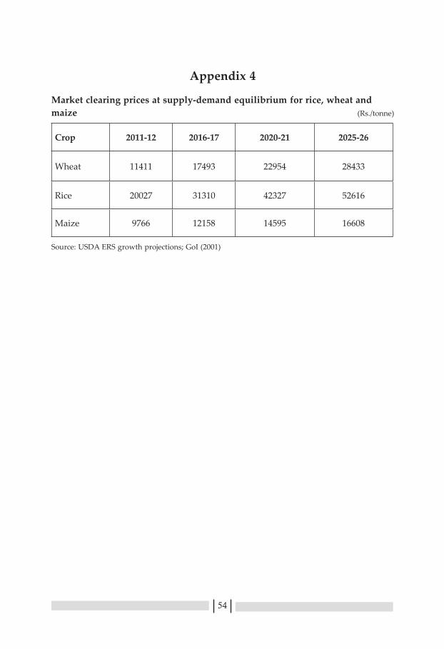
54

Appendix 4

Market clearing prices at supply-demand equilibrium for rice, wheat andmaize (Rs./tonne)

Crop 2011-12 2016-17 2020-21 2025-26

Wheat 11411 17493 22954 28433

Rice 20027 31310 42327 52616

Maize 9766 12158 14595 16608

Source: USDA ERS growth projections; GoI (2001)

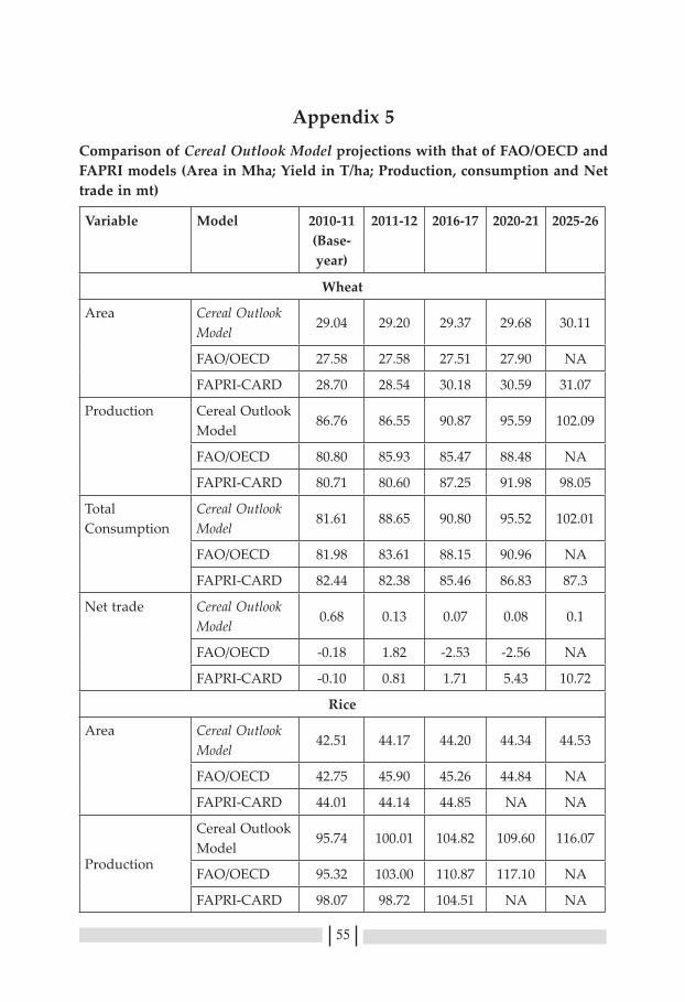
55

Appendix 5

Comparison of Cereal Outlook Model projections with that of FAO/OECD and FAPRI models (Area in Mha; Yield in T/ha; Production, consumption and Net trade in mt)

Variable Model 2010-11 (Base-year)

2011-12 2016-17 2020-21 2025-26

Wheat

Area Cereal Outlook Model

29.04 29.20 29.37 29.68 30.11

FAO/OECD 27.58 27.58 27.51 27.90 NA

FAPRI-CARD 28.70 28.54 30.18 30.59 31.07

Production Cereal Outlook Model

86.76 86.55 90.87 95.59 102.09

FAO/OECD 80.80 85.93 85.47 88.48 NA

FAPRI-CARD 80.71 80.60 87.25 91.98 98.05

Total Consumption

Cereal Outlook Model

81.61 88.65 90.80 95.52 102.01

FAO/OECD 81.98 83.61 88.15 90.96 NA

FAPRI-CARD 82.44 82.38 85.46 86.83 87.3

Net trade Cereal Outlook Model

0.68 0.13 0.07 0.08 0.1

FAO/OECD -0.18 1.82 -2.53 -2.56 NA

FAPRI-CARD -0.10 0.81 1.71 5.43 10.72

Rice

Area Cereal Outlook Model

42.51 44.17 44.20 44.34 44.53

FAO/OECD 42.75 45.90 45.26 44.84 NA

FAPRI-CARD 44.01 44.14 44.85 NA NA

Production

Cereal Outlook Model

95.74 100.01 104.82 109.60 116.07

FAO/OECD 95.32 103.00 110.87 117.10 NA

FAPRI-CARD 98.07 98.72 104.51 NA NA

56

Variable Model 2010-11 (Base-year)

2011-12 2016-17 2020-21 2025-26

Total Consumption

Cereal Outlook Model

90.21 96.55 100.81 105.72 112.03

FAO/OECD 91.42 95.55 106.86 112.84 NA

FAPRI-CARD 91.38 92.57 98.38 NA NA

Net trade Cereal Outlook Model

2.77 4.27 4.04 4.03 4.0

FAO/OECD 3.40 4.95 4.73 4.91 NA

FAPRI-CARD 4.44 5.76 6.75 NA NA

Maize

Area Cereal Outlook Model

8.61 9.04 9.26 9.19 9.14

FAO/OECD NA NA NA NA NA

FAPRI-CARD 8.20 8.61 7.80 7.57 7.35

Production

Cereal Outlook Model

21.84 23.72 25.26 26.31 27.20

FAO/OECD NA NA NA NA NA

FAPRI-CARD 20.00 20.24 18.03 18.33 18.61

TotalConsumption

Cereal Outlook Model

18.10 20.64 22.55 23.50 24.34

FAO/OECD NA NA NA NA NA

FAPRI-CARD 17.80 18.28 19.88 21.39 23.03

Net trade Cereal Outlook Model

3.48 3.16 2.72 2.81 2.9

FAO/OECD NA NA NA NA NA

FAPRI-CARD 2.00 1.86 -1.87 -3.07 -4.44

Note: For FAPRI-CARD Outlook on rice, the base-year is 2009-10; NA denotes ‘not available’. Source: Authors; http://www.fapri.iastate.edu/outlook; http://www.oecd.org/site/oecd-faoagriculturaloutlook.