poles and zeros of matrices of rational functions

Poles and Zeros of Matrices of Rational Functions

Bostwick F. Wyman*

Mathematics Department The Ohio State University

Columbus, Ohio 43210

Michael K. Saint

Department of Electrical and Computer Engineering

University of Notre Dame

Notre Dame, Indiana 46556

Giuseppe Conte

Department of Mathematics

University of Genoa

Genoa, Italy 16132

and

Anna Maria Perdon

Department of Mathematical Methods and Models

University of Padua

Padua, Italy

Submitted by Robert M. Curalnick

ABSTRACT

This expository paper considers the problem of defining poles and zeros with multiplicity, including those at infinity, for a matrix of rational functions over a field. The underlying theme question for the paper is: does the number of poles of a matrix

*Telephone: (614) 292-4901. E-mail: [email protected] or

[email protected].

‘The work of the second author was supported in part by a Distinguished Visiting

Professorship at the Ohio State University and in part by the Frank M. Freimann Chair in

Electrical Engineering at the University of Notre Dame.

LINEAR ALGEBRA AND ITS APPLICATIONS 157:113-139 (1991)

0 Science Publishing Co., Inc., 1991

113

655 Avenue of the Americas,

114 BOSTWICK F. WYMAN ET AL.

equal the number of zeros, and what structural meaning underlies such an assertion?

Our approach is motivated by ideas from linear system theory and control engineer-

ing. Control-theoretic ideas are not a prerequisite, and we hope to encourage

specialists in classical linear and commutative algebra to investigate this promising

source of new algebra problems.

1. INTRODUCTION

Suppose we are given a rectangular matrix G(Z) with coefficients in the field C(Z) of rational functions over the complex field C. What does it mean to say that a complex number A is a pole of G(z)? A zero of G(z)? How can we count the multiplicities of zeros and poles of a matrix? Should the number of zeros of a matrix equal the number of poles? Why should we ask such questions at all?

The one-by-one case is very familiar. Suppose f(z) is a rational function in C(Z), and write f(z)= u(~)/b(z) with polynomials a(z) and b(z) in lowest terms. Then the complex poles of f(z) are the roots of b(z) and the zeros of f(.~> are the roots of U(Z), counted with appropriate multiplicity. We can also decide if the “point at infinity” is a pole or zero of f(z), by setting

Then m is a zero of f(z) of order 6 if 6 is positive, and a pole of order - 6 if 6 is negative. Counting all points, including m, with proper multiplicity, we see that the total number of poles coincides with the total number of zeros. This common value, called the degree of f(z), is just the maximum of the degrees of the polynomials a(z) and b(z).

What happens if we are dealing with a matrix rather than a single function? We begin with an example to illustrate some of the issues involved. Let

=+3 -2(_7 +5)” Z(Z +3)

-+2 u G(z) =

(Z +1)(z +2) (Z +1)(2 +2)

1 z(.z +5)” Z

(Z +1)(.2 +2) z+2 (Z +1)(z +2) 1. It seems reasonable to say that A is a pole of G(z) if at least one

coefficient of G(Z) has a pole at A. This approach gives poles at A = - 1 and

POLES AND ZEROS 115

-2. Since the coefficients of the middle column have a pole at infinity, we could also make a case that G(z) has a pole at infinity.

What about zeros? We are used to saying that a matrix is “zero-like” if it has unexpectedly small rank. Over C(Z), G(z) has rank two, so that it has full row rank but deficient column rank. The null space of G(Z) gives a sort of “generic zero,” which we will discuss later. Right now we are concerned with identifying individual complex numbers (or perhaps infinity) which should be called zeros of G(z). If A is not a pole, we can compute G(A), and we will say that A is a zero of G(z) if the rank of G(h) [over C] is strictly less than the rank of G(Z) [over C(Z)]. Now G( - 5) has rank one, so -5 is such a zero.

So far we have not mentioned multiplicities for the zeros and poles of G(z). Counting these multiplicities correctly is rather subtle, and they are best viewed as dimensions of zero and pole spaces which are defined later in the paper. For now, we just state the answers for the example: - 1 and -2 are simple poles, 03 is a double pole, - 1 is a simple zero, and - 5 is a double zero. So far we have four poles and three zeros. There must be another zero lurking somewhere, and it turns out that it comes from the nullspace of G(z), measured by ideas that go back to Wedderbum and Kronecker. In any case, we will eventually conclude that the degree of G(Z) is four, and is given by the total number of poles, or the total number of zeros, and we call the common value the degree of G(Z).

In the rest of the paper we will give precise definitions of the notions of pole and zero of a matrix of rational functions. Our approach is motivated by ideas from linear system theory and control engineering. We will attach to each matrix G(z) a pole module and a zero module which correspond to state spaces of appropriate linear control systems. These objects are finitely generated torsion modules over C[Z] (for finite poles and zeros), which can be thought of as vector spaces equipped with square matrices which describe the dynamics of the systems involved. The eigenvalues of these matrices correspond to the naive poles and zeros discussed here in terms of loss of rank, and the modules themselves (or, equivalently, the Jordan form of the matrices) give good ways to measure multiplicities. The point at infinity can be treated in a strictly parallel way, replacing the ring of polynomials by the local ring of rational functions regular at infinity. We conclude by sketching a way of measuring “generic zeros” and explaining why, in a certain sense, the number of zeros really does equal the number of poles, even for a rectangular matrix.

We have tried to make the prerequisites for reading this paper as modest as possible. Although many of the ideas here are motivated by ideas of control engineering, no previous experience with control theory is assumed. The algebraic prerequisites are more substantial: a good command of linear


algebra over fields and the algebra of polynomials and rational functions is essential, and some acquaintance with the ideas of modules over principal- ideal domains (or at least polynomial rings) is also important. One of the best elementary sources for this material is the text of Hartley and Hawkes [6]. Many graduate algebra texts, such as [l, Chapter 141, treat this material in a broader context.

We would like to thank R. Guralnick for encouraging us to submit this article as an expository paper. Proofs are omitted or sometimes sketched very briefly. Readers interested in the technical developments should read [28] and the references cited there.

2. POLES AND LINEAR SYSTEMS

In this section we begin with a mathematical object called a linear dynamical system, and we attach to it a matrix of rational functions which describes the input-output behavior of the system. This process motivates the reverse procedure: start with a matrix of rational functions, and attach to it a space of poles which is the state space of an appropriate linear system.

A discrete-time linear dynamical system consists of three vector spaces: an n-dimensional space X of states, an m-dimensional space U of inputs or controls, and a p-dimensional space Y of outputs or measurements. These spaces are connected by three linear transformations: A : X + X (dynamics), B : U + X (input), and C: X -+ Y (output). The behavior of the system is defined by difference equations:

x(t+l)=Ax(t)+Bu(t),

y(t) =Cx(t).

A sequence of inputs {u(t)) produces a sequence of states {x(t)), which in turn produces an output sequence {y(t)). There is a continuous-time, or differential-equation version, which is more widely used in control engineering, but we will stick to the discrete-time form. In addition to its importance in engineering, the discrete-time case has a clearer algebraic intuition, occurs frequently in algebra and combinatorics, and generalizes to arbitrary fields of scalars.

To study the outputs resulting from a sequence of inputs, we introduce the generating function or g-transform of a sequence of vectors. For each t, let v(t) be a vector taken from some space V. Assume that {v(t)} is a

POLES AND ZEROS 117

sequence of vectors such that there is an integer N, such that v(t) = 0 for all t < N(u). We write

a vector formal power series. The exponent sign convention is perhaps a little unexpected, since z-’ indexes an event at time t, but this choice allows us to represent shifts into the past as multiplication by z. The polynomial part, or past history, of a(u) is

Tr+gqu)= : o(t)z-‘, t = LV,

which is nonzero only when N, < 0 and lives in the space V[z] of polynomials with vector coefficients. The strictly proper part

?T_gu> = f o(t),_-’ t=l

describes the future of the sequence u(t). When convenient, we can think of $)<ti> as a column vector of formal power series, r+ a(u) as a column vector of polynomials, and r_ $2(u) as a column vector of strictly proper power series.

Computations using the $2transform are based on straightforward linear- ity properties, together with the important shifi formula. If u(t) is a sequence of vectors in V, define a(u) by a(u)(t) = u(t + 1). Then, a routine computation shows that $?(a~) = za<u>. The defining equations for a system give

?(Y) = C9<~>7

so that a(y) = C(zZ - A)-‘By(u). We write G(z) = C(zZ - A)-‘& a matrix of rational functions, and call it the transfer function or transfer-function matrix. Let adj(zZ - A) be the classical adjoint of zZ - A, whose coefficients,


defined by various cofactors, are polynomials in z. Then, by Cramer’s rule,

(z1-AA)-1= de&A) adj( aI - A)

and

1 G(z) =

det( zI - A) Cadj(zI - A) B.

Since G(z) is a rational matrix, we will stop considering inputs and outputs which are arbitrary power series and only consider sequences whose transforms are rational. Thus a<~>, which we will write just as u(n) from now on, will be a column vector whose coefficients are rational functions in C(z). To consider a rational column vector as power series showing past and future part, we can simply expand it into powers of z-l by long division. If u(z) is rational and y(z) = G(z)u(z), then y(z) is also rational. We denote the spaces of rational vectors by U(z) and Y(z) and write our transfer function from now on as a C(z)-linear transformation G(z): U(z) + Y(z).

We would like to identify the poles of G(z) with the eigenvalues of the dynamics matrix A. Although this is not quite right, it is not completely unreasonable, either. The adjoint formula above shows that poles of G(z) are all roots of the characteristic polynomial det(zI - A) of A. On the other hand, it can happen that some factors of det(zI - A) cancel factors from C adj( zI - A) B, so that not every eigenvalue of A is a pole. For an easy but typical example, let

A=(; z2). B=(i), C=(l 1).

Then G(z) = l/(.z - A,), and somehow A, has been lost. One says that this system (A, B,C) is not a minimal system. The eigenspace for A, is not needed, and the same transfer function can arise from a system of smaller dimension.

A brief discussion of these ideas will clarify the connection between A and the poles of G(z) in general and will help us solve the redization

problem, which goes like this: Given G(z), find a state space X and a dynamics matrix A which describes the poles of G(z). A system (A, B,C) gives rise to a (&)-linear transfer function G(z): U(z) + Y(z) as above.

POLES AND ZEROS 119

In a short note published in 1965, R. E. Kalman introduced the algebraic method which we adopt here (see [7; 8, Chapter 10; 201). A Kulman input-output map considers only input strings which end at time t = 0 and examines the resulting output only for time t > 1. These decisions translate into $)-transforms as follows: Let u(z)= u_,zn + . . . + u_1.z + ug, ui in U, be a polynomial input, and write the output as G(z)u(z) = y_,,+rzn-’ + . . . + Y_~Z + y. + ylz-’ + . . . + yt.ft + . . . , which is a rational column

vector expanded in powers of z - ‘. We define the Kalman output G#u(z) by considering only the strictly proper part G#u(.z) = r_G(.z)&) = yrz-’ + . . . + YtZ-f + . . . . How should we view G#? Its domain is the free module

U[Z] of vector polynomials, or equivalently the set of m X 1 column vectors with coefficients in ~[z]. We adopt Kalman’s original notation and call the domain s2U, viewed as a free module of rank m over C[z].

To find the range of G# we need to do a computation. Start with

G#(zu(z)) = ~_G(z)(zu(z))

= r_zG(z)u(z)

= *_(y,+y,=-‘+ ... +y,a-‘+‘+ -)

= yz”-l + y3/ + . . . + y,g+1+ . . .

Now the right-hand side is not quite zG#(u(z))= y1 + yaz-’ + . . . +

Ytu” --t+1_... . On the other hand, our original difference-equation intuition involved outputs for t 2 1 only, so we feel that the y1 term doesn’t really belong there. We repair the situation by introducing the Kalman output

module IY = Y(z)/RY. The space IY consists of equivalence classes of rational vectors where two rational vectors are equivalent if their difference is a polynomial vector. We declare the past irrelevant to outputs, identifying two rational outputs in IY if they coincide for all future times t > 1. Each class in IY has a unique strictly proper representative, and sometimes we identify TY as a set with the set of all such strictly proper vectors.

To define a suitable module structure on TY, consider RY as a C[z]-submodule of Y(z), so that the factor space IY inherits a module structure defined explicitly as follows. For y in TY, write

7 = ylzz-’ + . . . + ytzpf + . * * (mod CnY),

120

so that

BOSTWICK F. WYMAN ET AL.

zy = IJ~Z-~ + * *. + tjtzPt + * * * (mod fir),

which can be described as “shift left and erase the coefficient which fell into the past.” This action is exactly what we need to make sense of G#. Our structures have been designed so that given a system (A, B,C), the Kalman input/output map G . #. s1Y + TY is a C[z]-module homomorphism.

Since we have singled out the time t = 0 for special consideration, we can factor G” into two mappings involving the state space. We define them intuitively first, and then give formulas. Let B-: RU + X and C- :X -+ IY be given by

B-(polynomial input string) = resulting state at time t = 1, assuming that the initial state is zero when the input starts,

C-(state at time t = 1) =resulting output string for t > 1.

From this construction, we expect that GX = C- B-. To compute a future output from a past input, first make the appropriate state with B- and then

compute the output from the state with C-. To verify this maneuver using formulas, write

B-( u_n~n + . . . + u_,t + u”) = A”Bu_, + . . . + ABC, + Bu,,

c-(x) = Cxz-’ + C.&r-" + . . . + CA”-lx~-” + . . . ,

G#(u,) = CBu,z-’ + CABu,z-” + CA2B~,~-3 + . . .

To save notational agony, we have just written the formula for G# on U. Since G” is a C[z]-module map, this suffices to determine G# on any vector polynomial. It is also enough to check G” = C- B- on any vector in U, and this follows from the formulas.

We can summarize all this as the commutative realization triangle in Figure 1. So far we know that G # is a C[z]-module homomorphism given the free module structure on RU and the new structure on IY. If we make the state space X into a module by defining p(z)r = p(A)x for all p(z) in C[z], then the formulas also show that B- and C- are C[z]-module homo- morphisms. Thus the realization triangle is a module-theoretic diagram, and

POLES AND ZEROS 121

FIG. 1.

in fact it connects three very different kinds of modules. The past-input module is free; the state module is finitely generated and torsion. The future-output module can be shown to be divisible and torsion. This diagram, discovered around 1965, is the first indication that module language is valuable for the study of linear system theory.

Perhaps it is now time to remember that we started all this because some of the eigenvalues of A could fail to be poles of G(z). In the notation of the realization triangle, we say that the system (A, B,C) is reachable if B- is onto, i.e. if every state can be reached with a polynomial input. The system is observable if C- is one-to-one, so that every nonzero state eventually produces a nonzero output, and canonical if it is both reachable and observable. A concrete statement of the main result in this circle of ideas goes like this:

THEOREM. Suppose (A, B, Cl is a canonical system. Then every eigenvalue of A is a pole of some coefficient of G(z) = C(zI - A)-‘B. Furthermore,

zj (A,, B,, C,) is any system with the same transferfunction as (A, B,C), then

the size of A, is rw smaller than the size of A. lf A I has the same size as A, then (A 1, B,, C,) is also a canonical system, and A and A 1 are similar matrices.

Proofs of this theorem appear in many contexts. An early treatment can be found in [8, Chapter lo], and many papers in [12] deal with generaliza- tions of this approach. According to the theorem, canonical systems with a given transfer function are the systems of smallest size with that transfer function, and so they are commonly called minimal systems. If (A, B, C) is a minimal system with transfer function G(z), then the state space X, viewed as a C[z]-module using the matrix A, is (up to similarity) a uniquely determined object which describes all the poles of G(z). Looking again at the realization triangle, we see that since X is the image of B-, we can write X E fiU/ker B-. Furthermore, since C- is one-to-one, it follows that ker B- = ker G#. To compute kerG# exactly, note that for a polynomial vector u(z) in RU, G#(u(.z))= 0 in IY if, and only if, G(z)u(z) is a polynomial in RY. That is, ker G# = G-‘(KIY)n RU, and the minimal state


space is given by X E flu/G-‘(flYIn RU. We hope that this is enough motivation for our first definition.

DEFINITION. Given a C(z)-linear transformation G(z): U(z) + Y(z), then the pole module ofG(z) is the C[z]-module X(G)= au/G-‘(fiY)n flu.

Consider the single-transfer-function case G(z) = u(z)/b(z.> in lowest terms, for which RU and RY are both just k[,-1. Since a(=) and b(z) are relatively prime, one shows that G-‘(RY)n s1U= b(z)k[z] and X(G)= k[zI/&)k[=], giving a space with dimension equal to the degree of b(z). If the powers of u” are chosen as a basis, then the action of : gives a companion matrix of b(z) for the dynamics matrix A, so the poles of G(z) are the roots of b(z) and the eigenvalues of A.

More generally, for any G(z), X(G) is finite dimensional over C, with a dynamics matrix A induced from the C[z]-action. The space X(G) fits into a realization triangle, so that B and C also appear, and C(zl - A)-‘B is the strictly proper part of the original G(z). The polynomial part of G(z), if any, has no effect on X(G). (Polynomials only have poles at infinity. See Section 5 below for that theory.) The dimension of X(G) is called the McMih degree, after the circuit theorist Brock McMillan, or simply the degree. The eigenvalues of A are called the poles of G(z), and their algebraic multiplicities as eigenvalues are defined to be their multiplicities as poles of the system.

This concludes for a while our study of poles of a matrix of rational functions. We have given a rigorous definition which mirrors the intuitive notion of poles of the coefficients, and we have made clear what we mean by the multiplicity of a pole. Our ideas have been incorporated into the definition of a pole module, and Section 4 will contain some material on explicit computations of pole modules. Meanwhile, in the next section we begin studying the zeros of a matrix of rational functions.

3. ZEROS OF A RATIONAL MATRIX

Suppose G(z): U(z) + Y(z) is a transfer function. A vector u(z) in U(z) such that G(,-)u(=) = 0 should surely be called a zero of G(z). The set of such zeros, the null space of G(Z), gives too little information, and to proceed we call a vector u(z) a zero if the future output string is given by r._ G(z)&) = 0. Since u(z) will be a zero if G(z)&) lies in the module RY of polynomial output vectors, our study of zeros begins with the set G-‘(fly).

POLES AND ZEROS 123

The pole module X(G) arises as the quotient of a free module of input

strings modulo a free module of “trivial inputs.” Is there a suitable “trivial

submodule” in the theory of zeros? Since outputs are considered zero-like if

they are confined to the past, why not consider past inputs equally trivial?

This philosophy leads to a new construction

Z,(G) = _ G-‘( RY)

G '(RY)nRU

which is a space of classes of inputs which give trivial outputs, modulo trivial

inputs. The module Z,(G) might not be finite dimensional, having an

infinite-dimensional part coming from the honest zeros in the null space of

G(z). The nullspace ker G(z) in U(z) is a C(z)-vector space and very large

when viewed over C[z]. Since kerG(z)cG-‘CRY), we can define a sub-

space of Z,(G) by

ker G(z)

z0(G)= (kerG(=))nflU’

Now Z,,(G) is infinite dimensional over C, but if we just kill it off we are

left with a very useful finite-dimensional space of zeros called the trunsmis- sion zero module of G(z). Define, following [25],

G(G) Z(G) =-=

G-'( fly) + s2U

Z”(G) kerG(,-)+RU ’

For motivation, we compute the transmission zero module of a single transfer

function G(z) = &)/b(z) in lowest terms. In this case, kerG(z) vanishes,

and

G-'(RY)= u(z)~C(z): i

u(z) -u(z) = p(z) E c[z] , b(=) I

G-'(RY)+RU= i b(z)dz) u(_) +YwP(h7w=Cbl

u i

= b(z)p(=) + 4,-)y(z) u(z)

:P(z),Y(z) EC[Zl

1 = -c[z],

u(z)


where the last step follows because u(z) and b(z) are relatively prime and

any polynomial r(z) can be expressed as h(z)&)+ &)cl(-“). To summa-

rize,

1

Z(G) = G-‘(C[z]) + C[z] u(z) ‘[,-I CL=1

c[z] = c[z] = u(z)C[z] .

That is, the zero module of the transfer function a(=>/&> is just the cyclic

module obtained by factoring out the numerator. The action of z on this

space gives a companion matrix of a(z), so the eigenvalues are just the roots

of a(z), as expected. A multivariable generalization of this computation will

be outlined in the next section.

Let G(z) be a transfer function with transmission zero module Z(G), and

let A, be the dynamics matrix obtained from the action of 2 on Z(G). For

every complex number A let z,(A) be th e g eometric multiplicity of A as an

eigenvalue of A,. That is, zc; (A) is zero if A is not an eigenvalue; otherwise

z,(A) is the dimension of the space of eigenvectors of A, for the eigenvalue

A. Although +;(A) ‘. IS no really a good measure of the multiplicity of the zero t

of G(z) at A, at least z,(A) is strictly positive exactly when A is a zero of

G(z). The number s,(A) 1s exactly what is needed to quantify the “rank-drop”

philosophy of the introduction. In fact, if A is not a pole of G(z) [so that

G(A) makes sense], we have rank, G(A) = rank,,,, G(z) - ,-,;(A). We will

give some indication of the proof of this formula in the next section.

4. COMPUTATIONS OF POLE AND ZERO MODULES

In this section we would like to describe some explicit methods for

computing the pole and zero modules of a transfer function G(z) : V(z) +

Y(z). The first method depends on the Smith-McMiElun form, a diagonal form

generalizing the classical Smith form of a polynomial matrix. Given the

p X m matrix G(z), there exist square polynomial matrices L(z) and R(z)

with nonzero constant determinants such that

fl(Z) 0 ... 0

L(z)G(z)R(z) = fids) y ; , . . .

f,(z) 0 I

POLES AND ZEROS 125

drawing the picture for p < m. [Proof: Clear denominators to get P(Z) = dig for some d(z), then do the Smith form for the polynomial matrix P(Z), and finally divide by d(z).] Here the f&) can be taken as rational functions of the form e,(=)/d,(-) 1 m owest terms with divisibility relations

e,(z) I e,(z) I . . * I e,(z) and d,(z) I d,_,(z) I . . . I d,(z). (See 115, pp. 109-110; 9, Chapter 61). The di(z) are called the pole polynomials, and the e,(z), known as the Rose&rock zero polynomials, were historically the first good definition of multiplicity for multivariable zeros. Their importance is indicated in the following theorem from [25].

T~IEOHE~. The pole polynomiuls are the invariant factors of the pole

module X(G), and the zero polynomials are the invariant factors of the zero

module Z(G).

The upshot of this theorem is that the pole polynomials and the zero polynomials determine the pole and zero modules up to isomorphism. Consider again the example

z+3 -2(Z +5)” Z(Z +3)

G(Z) = (Z +l)(Z f2) (Z +2) (Z + l)(Z +2)

1 Z(Z +5)2 Z

(Z +1)(= +2) (Z +2) (-v7+1)(u?+2)

The Smith-McMillan form of G(z) is given by

1

G(-)= I (~+1)(,_+2) 0 0

0 (2 +1)(z +5) 2 0

which verifies the assertion made in the Introduction that G(Z) has poles at - 1 and -2 and zeros at - 1 and - 5 (double).

Another technique which produces concrete modules rather than just invariant factors is given by matrix-fraction methods, which involve some interesting noncommutative algebra. Let G(z) be a p X m matrix of rational functions. Then there exist a p X m numerator matrix N(z) and an m X m denominator matrix D(Z) such that:

(1) N(z) and D(t) have coefficients in the polynomial ring k[z]. (2) det D(z)# 0, so that D(z)-’ exists over k(z).

126 BOSI’WICK F. WYMAN ET AL.

(3) G(s) = N(z)D(z)-‘. (4) There exist polynomial matrices A(=) of size m # p and B(z) of size

m f m such that A(-)N(=)+ B(z)&) = I,,,, the m X m identity matrix.

Property (4) is one way of saying that N(z) and D(z) are right coprime

matrices. There is a theory of greatest common right matrix divisors, and the only right divisor of D(z) and N(z) is I,,,. (See [9, Chapter 6; 231.) Matrix factorizations give concrete descriptions of the pole and zero modules as follows:

THEOREM. Suppose G(z) = N(z)D(z)- ’ is a right coprime matrix fac-

torization. Then the polynomial pole module X(G) is ginen by X(G) g X( D - I) and X(0-‘> z QU/ D(z)RU. The polynomial zero module Z(G) E Z(N),

and Z(N) is the finite-dimensional part of fiY/ NRU. In fact fiY/ NRU E

Z(N)@ k[z]‘J-r, where p is the dimension of Y and r is the rank of G(Z).

Most of the proof can be found in [25]. We do not include details here, but the ingredients for the assertions about zeros include the fact that ker G(z) = ker N(z) since D(z) is nonsingular, and that the use of the function u(z)* D(z)u(z) maps N(z)-‘(LRY) to G(a)-‘(fly), inducing an isomorphism from Z(N) to Z(G). The matrix N(z) is a lot easier to deal with than G(z), since it defines a mapping between two free polynomial modules, and for vectors u(z) and y(z) in these modules the numerical vectors u(h) and U(A) are defined for all A.

For the matrix G(z), we can factor G(z) = N(z)D(z)-‘, where

N(z)= -:O [ -(,_+1)(z+5)” --z ,

0 0 I

(=;+1)(=+2) -2(2+1)(2+5)” --2

D(z) = 0 1 0 I . 0 0 1

The matrices D(z) and N(z) are right coprime and have the zero and pole modules as cokemels. A different factorization “at infinity” must be used to study the zero and pole behavior there, and this work will be done in Section 6 below.

Our last task in this section is to examine the rank-drop formula presented earlier.

POLES AND ZEROS 127

THEOREM. If G(z) is a transfer function and A is not u pole of G(n) (so that G(h) makes sense), we have rank, G(A) = rank..,, G(z)- z,(A). More generally, ij G(z)= N(z)D(z)-’ is a right coprime matrix factorization,

rank, N(A) = rankC.Zj N(Z)- +(A), so thut the rank drops exactly when A is un eigenualue of the transmission zero matrix A,,, and the value of the drop is the expected amount z,(A).

To sketch the proof, consider the isomorphism flY/2vflU g Z(N)@ k[u”]P-’ from the last theorem. We can reduce this isomorphism modulo the polynomial = - A. This operation is done formally by a tensor product, but is morally equivalent to substituting A for = whenever possible. Only the space of A-eigenvectors of the matrix A,, acting on Z(N) survives, and we call this part Z(N)(A). We get Y/N(A)U= Z(NXA)@k”-‘. Counting dimensions, we get p -rank N(A) = =,(A)+ p - r, and rank N(A) = r - z,(A). Since D(Z) is nonsingular, r = rankc(-_) G(z), and also rank, N(A) = rank, G(A) whenever D(A) # 0.

5. ZEROS, POLES, AND FEEDBACK

Transmission zeros have been widely used in the control-theory literature. A classical view of their use in single-input, single-output design is given in [17], and Rosenbrock [15] is the primary source for multivariable zero theory. For a historical survey with many citations see [16]. Here, we would like to discuss only one issue-how the zero module appears as a subspace of the pole module. It turns out that this point of view is closely related to the theory of feedback in linear control systems and leads naturally to a systematic way of counting the zeros and poles of a matrix.

Throughout this section we denote by G(z) a strictly proper matrix of rational functions, postponing until later the study of improper matrices. We have defined two modules so far: the pole module X(G) and the transmission zero module Z(G). The pole module with its dynamics matrix A is the state space of the minimal system which realizes the given input-output behavior properties. The zero module with dynamics matrix A,, can be viewed as a new state space which captures a different aspect of the given G(z).

In the case where G(z) = a(z>/b(z) is a single rational function, we know that X(G) has dimension equal to the degree of b(z) and that Z(G) has dimension equal to the degree of u(z). If G(z) is strictly proper, then Z(G) is smaller than X(G). Our next goal is to show that Z(G) is no larger than X(G) in general.


THEOREM 1261. Suppose that G(z) is strictly proper. Then there are two naturally defined subspaces V* and R* of X(G), and there is a C-linear isomorphism p: Z(G) + V*/ R*. In particular, dim Z(G) = dimV* -dim R*, which is no larger than dim X(G).

TO give a brief indication of the proof, begin by reviewing the two definitions

G-‘( fly) nu Z,(G)= _

G l(flY)nflU and X(G)= _

G ‘(RU)nRU’

Consider a rational vector u(z) in G-‘(RY) which represents a member of Z,(G). Then the polynomial part r+(u(,r)) represents a state in X(G). The map induced by u(z) + r+(u(z>) is well defined, since the “denominator modules” in the two definitions are the same. Thus we have defined a mapping p,: Z,(G) + X(G). Note carefully that p is only C-linear, not a C[z]-module homomorphism. Also, p is not necessarily one to one, since, for example, Z,(G) might be infinite dimensional.

Consider next the space

kerG(z)

Zo(G) = (kerG(z)) f’ RU

and the finite-dimensional lumped zero module

Z,(G) Z(G)=-=

G-'( fly) + flU

Z,(G) kerG(z) + OU

introduced in Section 3. The image p(Z,(G)) is a very important subspace V* of X, called the maximal controlled invariant subspace of X, and the

image p,(Z,(G)) is the corresponding maximal controllable subspace R*.

These two spaces play a crucial role in the study of feedback systems, which will be described below. Meanwhile, the important point is that p, induces an isomorphism of vector spaces p : Z(G) + V*/ R*.

The spaces V* and R* are cornerstones of an extensive subject called geometric control theory developed by Basile, Marro, Wonham, and Morse.

POLES AND ZEROS 129

See [24] for an elaborate treatment. To understand their significance, consider a minimal system (A, B,C). The null space W of C will not be A-invariant, since otherwise a state in W would stay in W for all time and be unobservable, contradicting minimality. Nevertheless it may be possible to alter A by feedback so that W is invariant under the new dynamics. For this purpose, a feedback is a map F : X + U assigns an input to each state. Given a feedback, control theory is the design of feedbacks

matrix. We are considering problem in which the new A + BF must also leave W invariant.

largest subspace V* in W such that an F can be found which leaves V” invariant.

desired Not but in any case there is a subspace R* of V* such that F can be chosen so that A + BF leaves V* and R* invariant desired eigenvalues

exactly given by the polynomial-

between Z(G) and the factor space V*/ R*. We are thinking of V*/ R* as measuring

mapping p is a C[.z]-module isomorphism between Z(G) and V*/ R*. In other words, the transmission changed by feedbacks respect the state constraint

relates Z(G) to the pole module X(G). The dimension

believe that, properly

section we figure out what the poles and zeros at infinity of a transfer example in the introduction enough; there are mysterious

present discussion,

similar difficulties failure of G(Z) to be surjective.

Section 7 below.


6. ZEROS AND POLES AT INFINITY

Suppose given a transfer function G(z): U(z) + Y(z), this time not necessarily strictly proper. An improper rational function is said to have a pole at infinity, so it is reasonable to say that G(z) has a pole at infinity if it has any improper coefficients. If infinity is not a pole of G(Z), then we can say that infinity is a zero if the rank of G(m) drops, just as before. Thus, every strictly proper matrix which vanishes at infinity presumably has lots of zeros there. This leaves us with all the problems we had before: how should we count multiplicities? What if the point at infinity is simultaneously a zero and a pole? What other structure can we find?

One great advantage of the algebraic approach is that by changing the ring of coefficients we get a new theory without altering the fundamental ideas. The ring c[,-] consists of all rational functions which are regular throughout the finite complex plane, and modules over C[z] have eigenvalues in the complex plane. The ring 0, of proper rational functions, those functions which have no pole at infinity, consists of rational functions &>/b(a) where a(,-) and b(z) are polynomials and the degree of h(z) is at least as large as the degree of a(=). The ring 0, is a principal-ideal domain which has a unique maximal ideal m, = (l/z)O, consisting of all strictly proper rational functions, and every nonzero ideal is a power of m,. Modules of proper rational vectors given by R,U = O;l’ and R,Y = 0: replace the modules of polynomial vectors.

In exact analogy to the polynomial case, the pole and zero modules of G(z) at infinity are given by

X,(G) = QJJ

fl,UnG-'(R,Y) ’

Z,(G) = G-‘( &Y) + s1,U

kerG(z)+R,U ’

Both of these modules are finite-dimensional vector spaces over C, and we say the dimension of X,(G) is the number of poles ofG(z) at infinity, while the dimension of Z,(G) is the number of zeros of G(z) at infinity.

We need to spend a little time studying finite-dimensional O,-modules. Suppose V is such an O,-module. Define a linear transformation J : V -+ V by J(U) = (l/z)z), which is reasonable, since l/z is in 0, and therefore acts on V. The annihilator of V is the ideal of all members of 0, which kill all the vectors in V. In the polynomial theory, this ideal is a principal ideal

POLES AND ZEROS 131

generated by the minimal polynomial of the matrix A which describes the action of .a. In the 0, situation, it must be some power of m,, say rnk. That is, l/z’ and therefore J’ kills V, so that J is a nilpotent transformation. This also makes sense in a very informal way as follows: since we are studying the point at infinity, the map induced by z on V (which of course does not exist) has a single “eigenvalue” equal to infinity, the only eigenvalue of I/Z is zero, and J must be nilpotent. Conversely, if J: C” -+ C” is a nilpotent linear transformation, then the formula (l/.z)x = Jx for x in C” defines an O,- module structure. Thus, every finite-dimensional O,-module is essentially a vector space together with a nilpotent map.

The study of the behavior of a linear system at infinity, especially for single-input, single-output systems, is classical in the engineering literature, often under the name high-gain theory. Work on multivariable systems related to poles at infinity can be found in [18, 19, 10, 11, 141. The O,-module point of view was first developed in [2, 31 and continued in [21].

To compute the pole and zero modules at infinity for a single function, let

g(z) = a(z)/b(z), and let 6 = degree b(z) - degree a(z). At infinity, g(z) has a zero of order 6 if 6 is positive, and a pole of order - 6 if 6 is negative. To see how this shows up in the module definitions, look at

L(g) = 0,

0, n C’(OJ

If 6 is positive, g is strictly proper and g-‘(0,) = O,, so X,(g) is zero. If 6 is negative, one can show that g-‘(0,) is exactly rn,‘. That is, X,(g) = 0,/m: is a &dimensional vector space on which I/Z acts nilpotently with a single 6 X 6 Jordan block. The zero module computation is exactly the opposite, giving zero if 6 is negative and an &dimensional space if 6 is positive.

Suppose next that G(Z) is an arbitrary p X m matrix of rational functions. How can we find the pole and zero modules at infinity? Once again we are saved by algebra. The matrix-fraction approach advertised in Section 4 above works over the polynomial ring C[Z] b ecause C[Z] is a principal-ideal domain. Now 0, is also a principal-ideal domain, so our earlier discussion should go through without much change. We can find a right coprime factorization G(z) = N,(z)D,(z)-‘, where N,(Z) and D,(z) are m X p and m X m matrices over O,, and D,(z) has nonzero determinant. Furthermore, we can assume that there exist matrices A(z) and B(z) over 0, such that

A(z)N,(z) + B(z)D,(z) = I,,.


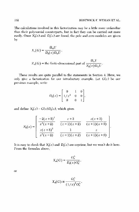
The calculations involved in this factorization may be a little more unfamiliar than their polynomial counterparts, but in fact they can be carried out more easily. Once N,(Z) and D,(Z) are found, the pole and zero modules are given

by

X,(G) = fuJ

D,( z)n,u ’

Z,(G) = the finite-dimensional part of QJ

N,( Z)R,U .

These results are quite parallel to the statements in Section 4. Here, we only give a factorization for our introductory example. Let G(Z) be our previous example, write

0 1 0

D,(Z) = [ l/Z” 0 0 1 ,

0 0 1

and define N,(Z) = G(Z)&(Z), which gives

-2(Z t-5)” ,_+3 Z(Z +3)

N,(z) = Z”(Z +2) (Zfl)(Z-t2) (z+l)(z+2)

Z(,” +5)” 1 Z

Z”(Z +2) (z+1)(z+2) (z+l)(z+2)

It is easy to check that N,(Z) and D,(Z) are coprime, but we won’t do it here. From the formulas above,

or

X,(G) = 02 (l/#O, ’

POLES AND ZEROS 133

which is a two-dimensional vector space. As for zeros,

Z,(G) = 0,

N,( z)Om” ’

which is zero, since N,(z) is surjective. Altogether this shows that G(z) has a double pole and no zero at infinity, as we asserted in the Introduction. A Smith-McMillan calculation is also available at infinity, but we omit it here.

We have tried to give the flavor of the theory of the pole and zero modules at infinity. These two modules are finite-dimensional vector spaces whose dimensions give appropriate counts of the number of poles or zeros. The module structure gives a nilpotent linear transformation whose invariant factors can give important additional structural information. Finally, we are omitting completely the “control and feedback’ aspect of the theory at infinity, mainly because it is rather complicated and still not completely understood. (But see the references mentioned above, especially [ll].) In particular, the realization space at infinity on which difference or differential equations evolve most naturally is a little bigger than the infinite pole module discussed here.

7. GLOBAL AND GENERIC ZEROS

Given a p X m matrix G(z) of rational functions in C(z), we have defined four modules: pole modules in the finite complex plane and at infinity, and zero modules in the finite complex plane and at infinity. We can assemble these to form global pole and zero spaces by M(G) = X(G) @ X,(G), and H(G) = Z(G) @ Z,(G). Both of these global constructions are only vector spaces, since they are sums of modules over different rings, and there seems to be no sensible way to consider them as modules either over C[.z] or over 0,.

The dimension of X(G) is the total number of poles of G(z), or the global McMillan degree. The dimension of Z(G) is the total number of zeros. Recalling that one of our original goals is to show that the number of poles of a matrix equals the number of zeros, we can ask whether x(G) and h(G) have the same dimension. These dimensions don’t coincide in the 2 X3 example we have been considering, and the space Z(G) is smaller than X(G) in general, so we need to look around for some more zeros.


The new zeros come from the failure of G(z) to be one to one or to be onto, and there are contributions to the zero theory of G(Z) from the kernel and cokemel of G(Z) which we need to quantify. A serious difficulty faces us at once: both the nullspace ker G(z) and the cokernel Y(z)/G(z)U(Z) are finite dimensional over the function field C(Z) but infinite dimensional over C. However, we can attach interesting vector spaces to G(z) which are finite dimensional over C by a new method, which we call the Wedderburn-Forney

construction.

Suppose we are given a finite-dimensional vector space V over C with space V(Z) of rational function vectors over C(n). Think of V(Z) very concretely as a space of column vectors with coefficients in C(Z). With this identification we can define maps r+ : V(Z) + V[Z] and r_ :V(Z) + 2 -i&,(V) such that rr+ takes the (coordinatewise) polynomial part of a vector and r_ takes the (coordinatewise) strictly proper part. Now suppose that U is any C(z)-subspace of V(Z). We define the Wedderburn-Forney

space associated to IL by

w(a) = r+(k)

un v[z]

In other words, the Wedderbum-Fomey space W(L) consists of equivalence classes of vectors which are polynomial parts of vectors in L, modulo vectors in L which are wholly polynomial.

For any vector space L the space W(L) is finite dimensional, and its dimension is the sum of a set of numbers introduced by J. H. M. Wedder- bum in [22, p. 481, which partly explains the name.

We take a few lines to describe the ideas of Wedderburn. Any column vector O(Z) in V(Z) can be assigned a degree 6(u) as follows: if U(Z) is a polynomial vector whose coefficients have no common factor, then 6(v) is just the maximum of the degrees of the coefficients (as polynomials). In general, any U(Z) can be multiplied by a rational function f(z) so that

f<Z>U<Z> ‘. p ly 15 o nomial with no common factors, and we define 6(u) = 6(-j%). (For fancier definitions and more discussion, see [27, 28, 41.) Wedderbum proceeded as follows. Given L, choose a nonzero vector oi in 11 of least degree. Then, choose u, in iL which has least degree such that {o,, ve) is linearly independent. Proceed to find a “minimal” basis Jo,, . . . ,G,) with degrees e, < e2 < . . . < e,. The vectors are not uniquely determined by L, but the numbers ej, called the Wedderburn indices of IL, are. They measure the size of II in a rather mysterious way. The Wedderbum indices of the zero space are all zero, and so are the Wedderburn indices of V(Z), since the standard basis is minimal.

POLES AND ZEROS 135

A basic result in [28] asserts that

dimW([L) = e, + e2 + . . . + e,.

The Wedderbum indices themselves are associated with a certain natural filtration (an increasing sequence of subspaces) of W(L), and they are closely associated with various integers which arise in control theory: controllability indices, column degrees, and invariant factors of certain pole modules at infinity. It is beginning to appear that the filtered vector-space structure is a good substitute for module structures, which are unavailable for global pole and zero spaces. The study of filtrations on all these spaces is very much a topic of current research, and we will postpone more discussion until we understand them better.

The spaces W(L) and their dimensions supply a way to study the missing zeros we are seeking. In fact, the main theorem of [27, 281 states that

dimX(G)=dimZ(G)+dimW(kerG(=))+dimW(G(,-)U(z)).

In other words, the nullspace ker G(Z) supplies one new kind of zero, and the column space G(z)&), or really the failure of the equality G(z)U(Z) = Y(Z), supplies another. We can call these new zeros generic zeros. The ordinary “1 umped” zeros are related to places where some rank drops, while the generic zeros represent a drop in rank “occurring everywhere.” If dim W(ker G(Z)) and dim W(G(z)&)) are used to count the multiplicities of these zeros, then the equation above really does assert that the number of poles of G(Z) equals the number of zeros.

The numerical assertion has been known in slightly different language for a long time. The Wedderbum-Fomey spaces were not known, but the indices first occurred in work of Kronecker on matrix pencils. (See [9, p. 4611). The new contribution here is structural: there are explicit mappings of vector spaces connecting the global poles, the global zeros, and the two Wedderbum-Fomey spaces. First we show that the space W(ker G(z)) can be identified as a subspace of the global poles X(G). (If G(Z) is proper, then it becomes the controllability space R*, as in [26].) There is an injective map

X(G) Z(G)-’ W(kerG(=))

which is a globalization of the map p : Z(G) + V*/ R* discussed earlier in the feedback discussions of Section 5. This map is not surjective in general,


but its failure to be surjective is measured exactly by W(G(z)U(z)). That is, we have a short exact sequence

X(G) O-‘Z(G) -+ W(kerG(z)) +W(G(z)U(,-)) +O.

The numerical result above follows from this sequence by counting dimensions.

Thus, finally we have refined the attractive assertion “number of zeros = number of poles” into a powerful algebraic theorem which is intertwined with deep ideas of linear control and system theory. Furthermore, this new result and especially the rather mysterious Wedderbum-Fomey spaces have already suggested a number of new insights and new directions for research in the algebraic theory of linear systems.

8. THREE EPILOGUES

A. Forney and His Referees

J. H. M. Wedderburn is one of the famous algebraists of the century, and his contribution to the Wedderbum-Forney spaces has been discussed extensively in this paper. David Fomey, a well-known information theorist, wrote a paper [4] in 1971-72, eventually published in 1975, in which he rediscovered these ideas of Wedderburn, gave nice proofs (Wedderbum’s book, which Fomey did not know in 1975, is very sketchy), and applied them to linear system theory. In another manuscript written about the same time, Fomey introduced spaces more or less of the form W(L). Working from a faded and wrinkled preprint in early 1988, the present authors adapted these spaces and used them to study global poles and zeros as discussed here. However, in the treacherous journey between preprint and final published paper, the “ Wedderburn-Forney space” disappeared from Forney’s work. (At least, we can’t find it, and Fomey doesn’t remember.) We can just imagine some referee saying “this paper’s too long, and this part doesn’t seem relevant to the main ideas of the paper, so why don’t you take it out?’ In fact, the spaces didn’t have much to do with convolutional coding theory and linear systems over finite fields, the main subject of that paper. Furthermore, rather little was done with the idea there, so it was probably reasonable to drop the topic completely. On the other hand, if the authors of the present paper, excited about the ideas of zero modules, had not accidentally been reading an old preprint, what would have happened? Does peer review and

POLES AND ZEROS 137

the present system of scientific publication work well? How many other promising mathematical ideas have vanished, or almost vanished, on the cutting room floor?

B. Some History and a Few Citations The theory of poles and zeros of a single transfer function, primarily used

in conjunction with the Laplace-transform theory of continuous-time systems (those associated with linear time-invariant differential equations), has been used extensively since the 1930s to design amplifiers, motors, and all sorts of control systems. Alistair MacFarlane has written a nice historical summary [I3]. However, when more than one input or output were considered, the subject became more mysterious. Starting around 1960, Kalman and others revived a tradition going back to Maxwell’s steam-engine governors, and went back to explicit differential equations. An extremely powerful and attractive theory of linear control systems evolving in a state space was developed. This body of state-space methods has been so successful that most of us do not think of it as a theory, but simply as the way things are.

In his book [I51 published in 1970, Howard Rosenbrock studied zeros of multivariable systems, introducing the zero polynomials. Rosenbrock, Wolovich, and others ushered in a counterrevolution of refined transform methods, including the matrix-fraction techniques. Nowadays we need to move easily from one language and set of techniques to the other, exploiting their relationships and complementary strengths.

Kalman introduced the module-theory context which inspires the pole theory of the present paper around 1965 [7, 8, 201. The module-theoretic view of multivariable zeros was only introduced in 1980 [25]. The technical results on poles, zeros, and Wedderburn-Fomey spaces discussed in Section 7 can be found in [27, 281. There has been a steadily growing literature in this area, some of which is cited in the reference list, and algebraic methods are having an increasing influence on control theory. See the SIAM report

]5, p. 761.

C. But Is It Algebra.? Well, of course it’s algebra, with all those vector spaces and mappings.

And in this exposition we didn’t even get to the valuations which occur when the theory is done over a field which is not algebraically closed, nor did we mention that Wedderbum’s degree of a vector is also the degree of the corresponding embedding of the projective line into a big projective space. Better questions would be, is it mainstream algebra? Is it worthwhile? Are there good unsolved problems? To these we answer: “not yet, but maybe


soon, ” “absolutely,” and “lots.” Some of our favorite unsolved problems, with

an algebraic rather than an engineering flavor, are:

(a) What in the world is the Wedderbum-Fomey space really? It looks

vaguely like an algebraic-geometry construction, and the Wedderburn in-

dices have some connection with splitting vector bundles over the projective

line.

(b) What would a truly global system theory look like:? The theory of

lumped poles and zeros is local in the sense that they can be studied at each

complex number and at infinity individually.

(c) Can we generalize these ideas to fields of algebraic functions in one

variable of higher genus:? This is an attractive question in algebra, but it is

not particularly clear what engineering applications such a theory would

have. On the other hand, the theory of two-dimensional image processing is

related to polynomials and rational functions in two transcendentally inde-

pendent variables, so we could also ask about poles and zeros in that case as

well.

REFERENCES

1

2

3

4

5

6

7

8

9

10

11

12

P. Bhattacharya, S. Jain, and S. Nagpaul, Basic Abstract Algebra, Cambridge U.P., 1986.

G. Conte and A. Prrdon, Generalized state space realizations of non-proper

transfer functions, Systems Control L&t. 1 (1982).

G. Conte and A. Perdon, Infinite zero module and infinite pole modules, in VII

International Conference on Analysis und Optimization of Systems: Nice, Lecture

Notes in Control and Inform. Sci., 62. Springer-Verlag, 1984, pp. 302-315.

G. D. Fomey, Jr., Minimal bases of rational vector spaces with applications to

multivariable linear systems, SZAM J. Control 13:493-520 (1975).

W. Fleming (Ed.), Future Directions in Control Theory, SIAM, Philadelphia,

1988.

B. Hartley and T. Hawkes, Rings, Modules, and Lineur Algebru, Chapman and

Hall, London, 1970.

R. E. Kalman, Algebraic structure of linear dynamic systems. I. The module of

sigma, Proc. Nut. Acad. Sci. U.S.A. 54:1503-1508 (1965).

R. E. Kalman, P. Falb, and M. Arbib, Topics in Muthemuticul System Theory,

McGraw-Hill, New York, 1969, Chapter X.

T. Kailath, Linear Systems, Prentice-Hall, Englewood Cliffs, N.J., 1980.

D. Luenberger, Dynamic equations in descriptor form, IEEE Trans. Automat.

Control AC-22:312-321 (Mar. 1977).

F. S. Lewis and R. W. Newcomb (Eds.), Special Issue: Semistate Systems,

Circuits Systems Sign& Process. 5, No. 1 (1986).

E. G. Manes (Ed.), Category Theory Applied to Computation and Control,

Lecture Notes in Comput. Sci. 25, Springer-Verlag, 1975.

POLES AND ZEROS 139

13

14

15 16

17

18

19

20

21

22

23

24

25

26

27

28

A. MacFarlane, The development of frequency response methods in automatic

control, IEEE Trans. Automat. Control, 1979, reprinted in Frequency Response

Methods in Control Systems, IEEE Press, New York, 1979. M. Malabre, Generalized linear systems: Geometric and structural approaches, Special Issue on Systems and Control, Linear Algebra Appl. 122/123/

124:123-144 (19891. H. Rosenbrock, State Space and M&variable Theory, Wiley, New York, 1970. C. Schrader and M. K. Sain, Research on system zeros: A survey, Znternat. J.

ControE 50:1407-1433 (19891. J. G. Truxal, Automatic Feedback Control System Synthesis, McGraw-Hill, New

York, 1955. G. Verghese, Infinite Frequency Behavior in Generalized Dynamical Systems, Ph.D. Dissertation, Dept. of Electrical Engineering, Stanford Univ., Aug. 1978. G. Verghese, B. Levy, and T. Kailath, A generalized state space for singular systems, ZEEE Trans. Automat. Control AC-26:811-831 (Aug. 1981). B. Wyman, Models and modules: Kalman’s view of algebraic system theory, in

A. C. Antoulas (Ed.), Mathematical System Theory, 279-293, Springer-Verlag, 1991. B. Wyman, G. Conte, and A. Perdon, Zero-pole structure of linear transfer functions, in Proceedings of the 1985 Control and Decision Conference, Fort Lauderdale. J. H. M. Wedderbum, Lectures on Matrices, Amer. Math. Sot. Colloq. Publ. 17, 1934, Chapter 4. W. Wolovich, Linear Multivariable Systems, Appl. Math. Sci. 11, Springer-Verlag, New York, 1974. M. Wonham, Linear Multiaariable Control: A Geometric Approach, 3rd ed., Springer-Verlag, 1985. B. Wyman and M. K. Sain, The zero module and essential inverse systems, ZEEE

Trans. Circuits and Systems CAS-28:112-126 (1981). B. Wyman and M. K. Sain, On the zeros of a minimal realization, Linear Algebra

Appl. SO:621-637 (1983). B. Wyman, M. Sain, G. Conte, and A.-M. Perdon, Rational matrices: Counting the poles and zeros, presented at 1988 IEEE Conference on Decision and Control, Austin, Tex. B. Wyman, M. Sain, G. Conte, and A. Perdon, On the zeros and poles of a transfer function, Special Issue on Systems and Control, Linear Algebra Appl.

122/123/124:123-144 (1989).

Received ]une 1990;final manuscript accepted 18 December 1990

poles and zeros of matrices of rational functions

Documents