Polar Magnetic Field Topology

Andreas Lagg

Max-Planck-Institut fur SonnensystemforschungGottingen, Germany

Solar Orbiter SAP science goal #4 + PHI stand-alone science meetingMPS Gottingen, Oct 26+27 2016

1 / 21

Introduction

SOP #4

Objective 4: How does the solar dynamo work and drive connections between theSun and the heliosphere?

4.1 How is magnetic flux transported to andre-processed at high solar latitudes?4.1.1 Study the detailed solar surface flow

patterns in the polar regions, includingcoronal hole boundaries.

4.1.2 Study the subtle cancellation effects thatlead to the reversal of the dominantpolarity at the poles

4.1.3 Explore the transport processes ofmagnetic flux from the activity beltstowards the poles and the interaction ofthis flux with the already present polarmagnetic field.

4.1.4 Study the influence of cancellations at allheights in the atmosphere.

4.2 What are the properties of the magneticfield at high solar latitudes?

4.2.1 Probability density function (PDF) ofsolar high-latitude magnetic fieldstructures.

4.2.2 Basic properties of solar high-latitudemagnetic field structures.

4.2.3 Probe the structure in deep layers of theSun.

4.3 Are there separate dynamo processesacting in the Sun?

4.4 How are coronal and heliosphericphenomena related to the solar dynamo?

2 / 21

Introduction

SOP #4

Objective 4: How does the solar dynamo work and drive connections between theSun and the heliosphere?

4.1 How is magnetic flux transported to andre-processed at high solar latitudes?4.1.1 Study the detailed solar surface flow

patterns in the polar regions, includingcoronal hole boundaries.

4.1.2 Study the subtle cancellation effects thatlead to the reversal of the dominantpolarity at the poles

4.1.3 Explore the transport processes ofmagnetic flux from the activity beltstowards the poles and the interaction ofthis flux with the already present polarmagnetic field.

4.1.4 Study the influence of cancellations at allheights in the atmosphere.

4.2 What are the properties of the magneticfield at high solar latitudes?

4.2.1 Probability density function (PDF) ofsolar high-latitude magnetic fieldstructures.

4.2.2 Basic properties of solar high-latitudemagnetic field structures.

4.2.3 Probe the structure in deep layers of theSun.

4.3 Are there separate dynamo processesacting in the Sun?

4.4 How are coronal and heliosphericphenomena related to the solar dynamo?

2 / 21

Targets for PHI (stand-alone) high-resmagnetic field measurements

Introduction

Outline

Polar magnetic field measurements1 What are the difficulties?2 Why is it important?3 What do we know?4 What can we expect from PHI?5 How to operate PHI to maximize polar field

information?

3 / 21

Problems

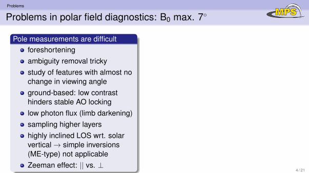
Problems in polar field diagnostics: B0 max. 7◦

Pole measurements are difficultforeshorteningambiguity removal trickystudy of features with almost nochange in viewing angleground-based: low contrasthinders stable AO lockinglow photon flux (limb darkening)sampling higher layershighly inclined LOS wrt. solarvertical→ simple inversions(ME-type) not applicableZeeman effect: || vs. ⊥

4 / 21

Problems

Problems in polar field diagnostics: B0 max. 7◦

Pole measurements are difficultforeshorteningambiguity removal trickystudy of features with almost nochange in viewing angleground-based: low contrasthinders stable AO lockinglow photon flux (limb darkening)sampling higher layershighly inclined LOS wrt. solarvertical→ simple inversions(ME-type) not applicableZeeman effect: || vs. ⊥

4 / 21

Problems

Problems in polar field diagnostics: B0 max. 7◦

Pole measurements are difficultforeshorteningambiguity removal trickystudy of features with almost nochange in viewing angleground-based: low contrasthinders stable AO lockinglow photon flux (limb darkening)sampling higher layershighly inclined LOS wrt. solarvertical→ simple inversions(ME-type) not applicableZeeman effect: || vs. ⊥

4 / 21

Problems

Problems in polar field diagnostics: B0 max. 7◦

Pole measurements are difficultforeshorteningambiguity removal trickystudy of features with almost nochange in viewing angleground-based: low contrasthinders stable AO lockinglow photon flux (limb darkening)sampling higher layershighly inclined LOS wrt. solarvertical→ simple inversions(ME-type) not applicableZeeman effect: || vs. ⊥

4 / 21

Problems

Problems in polar field diagnostics: B0 max. 7◦

Pole measurements are difficultforeshorteningambiguity removal trickystudy of features with almost nochange in viewing angleground-based: low contrasthinders stable AO lockinglow photon flux (limb darkening)sampling higher layershighly inclined LOS wrt. solarvertical→ simple inversions(ME-type) not applicableZeeman effect: || vs. ⊥

4 / 21

Problems

Problems in polar field diagnostics: B0 max. 7◦

Pole measurements are difficultforeshorteningambiguity removal trickystudy of features with almost nochange in viewing angleground-based: low contrasthinders stable AO lockinglow photon flux (limb darkening)sampling higher layershighly inclined LOS wrt. solarvertical→ simple inversions(ME-type) not applicableZeeman effect: || vs. ⊥

4 / 21

Problems

Problems in polar field diagnostics: B0 max. 7◦

Pole measurements are difficultforeshorteningambiguity removal trickystudy of features with almost nochange in viewing angleground-based: low contrasthinders stable AO lockinglow photon flux (limb darkening)sampling higher layershighly inclined LOS wrt. solarvertical→ simple inversions(ME-type) not applicableZeeman effect: || vs. ⊥

4 / 21

Durrant et al. (1981)

Problems

Problems in polar field diagnostics: B0 max. 7◦

Pole measurements are difficultforeshorteningambiguity removal trickystudy of features with almost nochange in viewing angleground-based: low contrasthinders stable AO lockinglow photon flux (limb darkening)sampling higher layershighly inclined LOS wrt. solarvertical→ simple inversions(ME-type) not applicableZeeman effect: || vs. ⊥

4 / 21

Durrant et al. (1981)

Problems

Problems in polar field diagnostics: B0 max. 7◦

Pole measurements are difficultforeshorteningambiguity removal trickystudy of features with almost nochange in viewing angleground-based: low contrasthinders stable AO lockinglow photon flux (limb darkening)sampling higher layershighly inclined LOS wrt. solarvertical→ simple inversions(ME-type) not applicableZeeman effect: || vs. ⊥

4 / 21

Durrant et al. (1981)

Problems

7◦ vs. 35◦ - continuum intensity

1•104

2•104

3•104

4•104

5•104

I C

Angle from Limb: 35˚ vs. 7˚

650 700 750 800 850 900 950X [arcsec]

−50

0

50

Y [

arc

se

c]

IC

IC

IC

5 / 21

Problems

7◦ vs. 35◦ - Stokes V

−0.006

−0.004

−0.002

0.000

0.002

0.004

0.006

V/I

C

Angle from Limb: 35˚ vs. 7˚

650 700 750 800 850 900 950X [arcsec]

−50

0

50

Y [

arc

se

c]

V/IC

V/IC

V/IC

6 / 21

Relevance

The importance of measuring polar B

Relevance for B at polar latitudespolar field is directly related to dynamo process(source of poloidal field)polar B field distribution responsible for coronalholes, polar plumes, X-ray jets, . . .Source of fast solar windSlow solar wind likely to emanate from CHboundaries

7 / 21

Polar magnetic fields: Basic properties (4.2.2.)

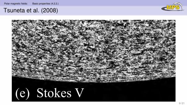
Tsuneta et al. (2008)

Best polar field measurementsTsuneta et al. (2008), Hinode SOT/SP

low straylight, stable space environmentB0 angle: 7◦ (2× per year)4.8 s integration time→ S/N ratio 1000 (increase to2000 is possible)

8 / 21

Polar magnetic fields: Basic properties (4.2.2.)

Tsuneta et al. (2008)

9 / 21

Polar magnetic fields: Basic properties (4.2.2.)

Tsuneta et al. (2008)

9 / 21

Polar magnetic fields: Basic properties (4.2.2.)

Tsuneta et al. (2008)

9 / 21

Polar magnetic fields: Basic properties (4.2.2.)

Tsuneta et al. (2008)

9 / 21

Polar magnetic fields: Basic properties (4.2.2.)

Tsuneta et al. (2008)

9 / 21

Polar magnetic fields: Basic properties (4.2.2.)

Tsuneta et al. (2008)

9 / 21

Polar magnetic fields: Basic properties (4.2.2.)

Tsuneta et al. (2008)

Analysis methodMilne-Eddington type inversions (MILOS code,Orozco Suarez et al., 2007)10 free parameters:

B, γ, φ - magnetic field vectorvLOS - line-of-sight velocityS0, S1 - source function & gradientη0 - ratio of line to continuum absorption coefficientsλD - Doppler widtha - the damping parameterα - stray-light factor

(similar to PHI onboard processing - no α)Q, U, or V signal ≥ 5σ (10.5% of all pixels)

10 / 21

Polar magnetic fields: Basic properties (4.2.2.)

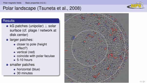
Polar landscape (Tsuneta et al., 2008)

11 / 21

Polar magnetic fields: Basic properties (4.2.2.)

Polar landscape (Tsuneta et al., 2008)

11 / 21

ResultskG patches (unipolar) ⊥ solarsurface (cf. plage / network atdisk center)larger patches:

closer to pole (heighteffect?)vertical (red)coincide with polar faculae5-10 hours

smaller patcheshorizontal (blue)30 minutes

Polar magnetic fields: Basic properties (4.2.2.)

Polar landscape (Tsuneta et al., 2008)

11 / 21

ResultskG patches (unipolar) ⊥ solarsurface (cf. plage / network atdisk center)larger patches:

closer to pole (heighteffect?)vertical (red)coincide with polar faculae5-10 hours

smaller patcheshorizontal (blue)30 minutes

Polar magnetic fields: Probability density functions (4.2.1)

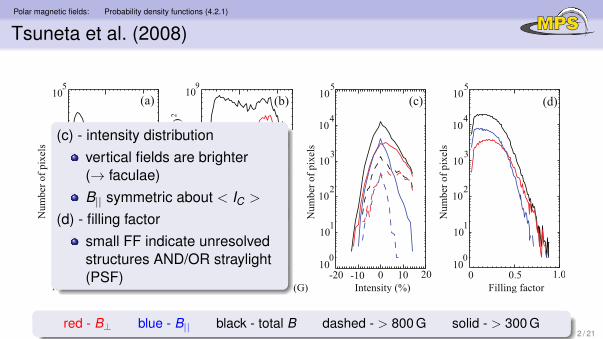
Tsuneta et al. (2008)

12 / 21red - B⊥ blue - B|| black - total B dashed - > 800 G solid - > 300 G

Polar magnetic fields: Probability density functions (4.2.1)

Tsuneta et al. (2008)

12 / 21red - B⊥ blue - B|| black - total B dashed - > 800 G solid - > 300 G

(a) - strength distributionB⊥ dominates strong fieldsB|| dominates weak fields

(b) - energy distribution (n × B2)weaker fields carry moreenergy

Polar magnetic fields: Probability density functions (4.2.1)

Tsuneta et al. (2008)

12 / 21red - B⊥ blue - B|| black - total B dashed - > 800 G solid - > 300 G

(c) - intensity distributionvertical fields are brighter(→ faculae)B|| symmetric about < IC >

(d) - filling factorsmall FF indicate unresolvedstructures AND/OR straylight(PSF)

Polar magnetic fields: Probability density functions (4.2.1)

Shiota et al. (2012): B-flux per patch number density

13 / 21

log(magnetic flux [Mx])

Polar magnetic fields: Probability density functions (4.2.1)

Shiota et al. (2012): B-flux per patch avg. flux density

14 / 21

Polar magnetic fields: Probability density functions (4.2.1)

Shiota et al. (2012): long-term study 2008-2012

15 / 21

vert. flux > 1018 Mx vert. flux < 1018 Mx

Polar magnetic fields: Two separate dynamos? (4.3)

Small-scale dynamo vs. global dynamo

Study small-scale flux emergencesmall-scale surface dynamo→ no latitudinal dependence expectedin-ecliptic measurements strongly biased:

foreshorteningsampled height leyerdifferent sensitivity for B⊥, B||small deflections in near-vertical field

evenly distributed measurements mandatory→ If PDF of properties (number, size, flux) are

significantly different at high latitudes⇒ strong support for weak features being due toglobal dynamo.

16 / 21

Polar magnetic fields: Two separate dynamos? (4.3)

Small-scale dynamo vs. global dynamo

Study small-scale flux emergencesmall-scale surface dynamo→ no latitudinal dependence expectedin-ecliptic measurements strongly biased:

foreshorteningsampled height leyerdifferent sensitivity for B⊥, B||small deflections in near-vertical field

evenly distributed measurements mandatory→ If PDF of properties (number, size, flux) are

significantly different at high latitudes⇒ strong support for weak features being due toglobal dynamo.

16 / 21

Polar magnetic fields: Subtle magnetic flux cancellation at the poles (4.1.2)

Details of cancellation mechanism

Flux removal at the polesWhat is the main mechanism? (Anusha et al., 2016)(death by disappearance of unipolar features,cancellation of bipolar features, merging events)PHI will deliver better estimate flux removal rate

17 / 21

Polar magnetic fields: Study of polar magnetic features (4.1.4.1.)

Special polar magnetic features (e.g. jets)

Example: details of polar jets (Quintero Noda et al., 2016)inversion of Hinode SOT/SP data after removing PSF effectheight-dependent inversion of Stokes profilesbest currently available comb. of data + analysis method

ResultsFaculae are ...

hot plasma tubes with low line-of-sight velocitiessingle polarity magnetic kG fields ⊥ solar surfaceslightly shifted wrt. continuum image towards the disc center

→ result of hot wall effectideal for combined measurements PHI & hi-res GB

18 / 21

Polar magnetic fields: Study of polar magnetic features (4.1.4.1.)

Special polar magnetic features (e.g. jets)

Example: details of polar jets (Quintero Noda et al., 2016)inversion of Hinode SOT/SP data after removing PSF effectheight-dependent inversion of Stokes profilesbest currently available comb. of data + analysis method

ResultsFaculae are ...

hot plasma tubes with low line-of-sight velocitiessingle polarity magnetic kG fields ⊥ solar surfaceslightly shifted wrt. continuum image towards the disc center→ result of hot wall effectideal for combined measurements PHI & hi-res GB

18 / 21

PHI observing modes for polar science

How to optimize PHI for measuring polar B?

Wishlist for polar B-field (standalone) sciencemax. solar latitudemin. distanceco-observations from Earth:

large B0 angle(March-08: South pole, September-08: North pole)ground-based support: Canary observatoriesSeptember preferable; DKIST?

HRT ME maps of all parametersfew Stokes parameter maps

19 / 21

PHI observing modes for polar science

Selecting good orbits: example #14

20 / 21

PHI observing modes for polar science

Bibliography

Anusha, L. S., et al. 2016, ArXiv e-printsDurrant, C. J., Kneer, F., & Maluck, G. 1981,

A&A, 104, 211Orozco Suarez, D., et al. 2007, Publications

of the Astronomical Society of Japan, 59,837

Quintero Noda, C., et al. 2016, MonthlyNotices of the Royal AstronomicalSociety, 460, 956

Shiota, D., et al. 2012, ApJ, 753, 157

Tsuneta, S., et al. 2008, ApJ, 688, 1374

21 / 21