HAL Id: hal-01119942https://hal.archives-ouvertes.fr/hal-01119942v1Preprint submitted on 24 Feb 2015 (v1), last revised 30 Mar 2016 (v4)

HAL is a multi-disciplinary open accessarchive for the deposit and dissemination of sci-entific research documents, whether they are pub-lished or not. The documents may come fromteaching and research institutions in France orabroad, or from public or private research centers.

L’archive ouverte pluridisciplinaire HAL, estdestinée au dépôt et à la diffusion de documentsscientifiques de niveau recherche, publiés ou non,émanant des établissements d’enseignement et derecherche français ou étrangers, des laboratoirespublics ou privés.

Polar Gaussian Processes for Predicting on CircularDomains

Espéran Padonou, O Roustant

To cite this version:Espéran Padonou, O Roustant. Polar Gaussian Processes for Predicting on Circular Domains. 2015.�hal-01119942v1�

Polar Gaussian Processes for Predicting on Circular Domains

E. Padonoua,b,∗, O. Roustanta

aMines Saint-Etienne, UMR CNRS 6158, LIMOS, F-42023 Saint-Etienne, France

bSTMicroelectronics, 850 Rue Jean Monnet, 38920 Crolles, France

Abstract

Predicting on circular domains is a central issue in many industrial fields such asmicroelectronics and environmental engineering. In this context Gaussian process(GP) regression is used, coupled with Zernike polynomials. However, usual GP mod-els do not take into account the geometry of the disk in their covariance structure(or kernel), which may be a drawback at least for technological or physical processesinvolving a rotation or a diffusion from the center of the disk. For that purpose, weintroduce so-called polar GPs defined on the non-Euclidian space of polar coordi-nates. Their kernels are obtained as a combination of a kernel for the radius usingan Euclidean distance, and a kernel for the angle, based on either chordal or geodesicdistances on the unit circle. Their efficiency is illustrated on two industrial applica-tions where radial and angular patterns are visible. In a second time, the problemof defining an initial design of experiment (DoE) for circular domains is considered.Two new Latin hypercube designs are obtained, by defining a valid maximin criterionfor polar coordinates. Their robustness in prediction is assessed and compared toother DoEs over a range of various toy functions and models.

Key words: Gaussian process regression, Polar coordinates, Circular domain,Design of Experiments

1. Introduction

This research aims at analyzing costly computer or physical experiments on a disk.The question was motivated by two industrial problems. In semiconductor produc-

∗Corresponding author.Email addresses: esperan.padonou@st.com (E. Padonou), roustant@emse.fr (O. Roustant)

Preprint submitted to — February 24, 2015

tion plants first, integrated circuits are produced on disks called wafers. Severaltechnological processes, such as lithography, heating or polishing, exploit the geom-etry of the disk, involving rotations or diffusions from the center. A common issueis to reconstruct a quantity of interest over the whole disk, from few measurementsat specific locations. The second problem is related to air pollution modelling forenvironmental impact assessment. Greenhouse gas concentrations are simulated bya computer code. Among the input variables, the couple (speed, direction) of windcharacteristics can be represented on a disk, the radius of which corresponds to themaximal speed. Here also, the goal is to predict the gas concentration from somesimulated experiments.

Approximation problems on the disk have been considered since the works of Zernike[1] in optics. Zernike polynomials are orthogonal with respect to the usual scalarproduct on the unit disk, a useful property for linear models. For such models,optimal design of experiments are known to be included in concentric circles [2].More recently, a stochastic model consisting of a Gaussian process (GP), also calledKriging model, has been proposed for microelectronics applications [3]. However itscovariance kernel, often simply called kernel hereafter, does not take into accountthe geometry of the disk, which may be a drawback, at least for technological orphysical processes involving a diffusion from the center of the disk, or a rotation.Indeed the prediction of a GP model is weighting more importantly the observedvalues corresponding to neighboring locations. With usual GPs, the neighbors arecomputed with respect to the Euclidian distance, which underestimates the influenceof points located on same concentric circles.

The main aim of the paper is to propose GP models that incorporate the geometry ofthe disk in their covariance kernel. For that purpose, we consider the parametrizationof the unit disk in polar coordinates: D = {(ρ cos θ, ρ sin θ), ρ ∈ [0, 1], θ ∈ S} where Srepresents the unit circle R/2πZ. The idea is to define a GP on the parametrizationspace C =]0, 1]×S defined by (ρ, θ). This implies constructing a kernel on a productof the Euclidian space ]0, 1] and on the circle S, which can be done by algebraicallycombining kernels on these two spaces with sum, product or ANOVA operations forinstance. The corresponding GPs will be called here polar GPs, and the usual onesbased on Cartesian coordinates, Cartesian GPs.

The construction of kernels on S can be achieved in several ways, and is connectedto the literature of directional data (see e.g. [4, 5]) and periodic functions (see e.g.[6]). One possibility is to use so-called wrapped GP [7], obtained by transforming amultinormal density to a periodic one by applying an operator written as an infinitesum. Here we focus on simpler approaches that provide explicit kernel expressions,

2

either by considering restriction to S of a 2-dimensional GP [6], involving the chordaldistance on S, or by using the recent results of Gneiting [8], involving the geodesicdistance on S. The geodesic distance on a general manifold was used recently bydel Castillo et al. [9] in the context of free-form monitoring, with so-called geodesicGPs. However, the goal and the approach are quite different here, where the formis fixed (the unit disk) and the geodesic distance known analytically. Furthermore,here the geodesic is relative to the manifold S which is only an algebraic portion ofthe mapped space C.

In a second time, we address the issue of defining an initial design of experiments(DoE) for circular domains. Considering the space C of polar coordinates is natural,but standard designs cannot be used directly due to its non-Euclidian structure.By considering a valid distance, we obtain maximin Latin hypercube designs (LHD,[10]) on C. That class of designs is recommended when the process has a physicalinterpretation in polar coordinates. In order to deal with more general situations,we also propose a modified version, which still has the LHD structure with respectto ρ and θ, and is well filling the disk D.

The paper is organized as follows. Section 2 presents the background and fixesnotations. Section 3 introduces so-called polar GPs. Section 4 shows the strength ofthe approach on two real applications, in microelectronics and environments. Section5 is devoted to designs of experiments. Two new LHDs are introduced and comparedto common designs, with respect to quality criteria. Their robustness in prediction isalso investigated on a set of toy functions and models. Section 6 discusses the rangeof applicability of polar GPs and gives perspectives for future research.

2. Background and notations

Denote D the unit disk represented either in Cartesian or polar coordinates:

D = {(x, y) ∈ R2, x2 + y2 ≤ 1} = {(ρ cos θ, ρ sin θ) , ρ ∈ [0, 1], θ ∈ S}

where S = R/2πZ is the unit circle. In various situations, one has to predict a variableof interest which is measured at a limited number of locations in D. For that purpose,we will consider the framework of Gaussian Process Regression (GPR) [6] also calledKriging in reference to its origins in geostatistics (see e.g. [11]). The measurementlocations, also called design points, will be denoted by X =

(x(1), . . . ,x(n)

). In GPR,

the observed values at X are modeled by:

Yi = µ(x(i)) + Z(x(i)) + ηi (1)

3

where µ is a trend function, Z ∼ GP (0, k) is a centered Gaussian process (GP) withcovariance function – or kernel – k, and η1, . . . , ηn are Gaussian random variablesrepresenting noise. We now briefly detail the three parts of the model.

The trend function µ is deterministic and often modeled as a linear combination ofbasis functions:

µ (x) = f (x)>β

where β is a vector of unknown coefficients. In our situation, Zernike polynomials[1] are good candidates for basis functions since they constitute an orthogonal basisfor the usual scalar product restricted to D. Their shape including regular patternsare also suited to describe symmetries or rotations, and have been recently used forpredicting on a disk by Pistone and Vicario [3].The stochastic part of model 1 comprises a GP and a noise. The GP Z takes intoaccount the spatial dependence, which thus entirely depends on its kernel k. Thechoice of k is crucial for applications, and may be done in order to include knowledgesuch as smoothness, periodicity, symmetries, etc. There are many ways to constructa kernel, and a comprehensive presentation is found in [6], Section 4. A key idea isthat multidimensional kernels can be obtained by algebraic operations, such as sumor products, of 1-dimensional kernels.Finally the noise part represented by the ηi’s may have two different purposes: Mod-elling a measurement noise, or adding flexibility. In this paper we assume that theηi’s are independent N(0, τ 2), where τ 2 is an unknown homogeneous variance termoften called “nugget”. When conditioning by the observed values, the model willinterpolate the observations if τ = 0 but not if τ > 0, which gives more flexibility.

When all parameters are known, prediction with Equation (1) is given in a closed formby a Gaussian conditional distributions knowing the observations Yi, i = 1, . . . , n.Its two moments are known as Kriging mean and Kriging variance. Analytical ex-pressions are also available when the parameters are estimated, known as universalKriging formulas (see e.g. [6] for more details), that we use here. An important factis that the Kriging mean at a new site x is obtained as an affine combination of theobserved values Yi, with weights depending on k(x,x(i)). Since k corresponds to thespatial dependence, the weights are more important for the x(i)’s that are close to xwhen this vicinity is measured by k.

4

3. Polar Gaussian processes

One way to define a GP on the unit disk D is to use the restriction of a GP onthe square [0, 1]2, defined in Cartesian coordinates. In this paper, we will call themCartesian GPs. Here, we propose to further exploit the geometry of the disk byusing the polar coordinates. The associated GPs will be callled polar GPs.

When using the polar coordinates, the unit disk D is connected to the cylinderC = ]0, 1]×S, where S denotes the unit circle, with the mapping, also called warpingin the context of GP modeling (see e.g. [6], Section 4.2.3.):

Ψ : (ρ, θ) ∈ C 7→ (ρ cos θ, ρ sin θ) ∈ D \ {0} (2)

This mapping is a one-to-one correspondence from C to the unit disk without itscenter. The fact that the center is lost in the mapping may be a problem in theory.In practice a design point located at the center of the disk can be replaced by a set ofdesign points placed on a closed concentric circle. A GP on D can then be obtainedby using Ψ−1, resulting in kernels on D ×D of the form:

k(x,x′) = kC(Ψ−1(x),Ψ−1(x′)

)(3)

where kC is a kernel on C × C.

Kernels on the cylinder can be defined by exploiting its product structure. This canbe done by combining a kernel kr on ]0, 1]×]0, 1] and a kernel ka on S × S. A firstway is by using the tensor product:

kprod (u,u′) = kr

(ρ, ρ′

)ka (θ, θ′) (4)

where u = (ρ, θ) and u′ = (ρ′, θ′) are in C. This formulation implicitly assumesthat Zu is the product of two independent components: a radial process Rρ and anangular process Aθ (Zu = RρAθ). It corresponds to a simple form of interaction. Forprocesses that do not have interactions between these components (Zu = Rρ + Aθ),an additive kernel should be more appropriate:

kadd (u,u′) = kr

(ρ, ρ′

)+ ka (θ, θ′) (5)

A trade-off between these two extreme approaches is the ANOVA kernel defined as:

kANOVA (u,u′) =(

1 + kr

(ρ, ρ′

))(1 + ka (θ, θ′)

)(6)

5

The expanded form of Equation (6) shows that a process Zu with ANOVA kernelcan be viewed as a sum of four independent GPs: a constant process Z0, a radialprocess Rρ with kernel kr, an angular process Aθ with kernel ka, and a process Z inter

on C with kernel krka. From the ANOVA point of view, these processes are similar toconstant term, main effects, and second-order interaction [12], but without respectingthe unicity constraints such as centering. Though out of the scope of this paper, aso-called KANOVA kernel mimicking exactly the ANOVA decomposition could havebeen proposed [13]. For more details on how to make new kernels from old, we referthe reader to [6].

Let us now define the kernels kr on ]0, 1]×]0, 1] and ka on S× S. We recall that validkernels must be positive definite. The domain ]0, 1] is a segment of a 1-dimensionalEuclidean space. As a consequence, traditional kernels are suitable for kr. In par-ticular, Matern kernels are attractive for their ability to control the smoothness ofthe process and to ensure numerical stability. In dimension 1, the Matern 5

2kernel

is given by:

km (x, x′) =

(1 +

√5 | x− x′ |

`+

5(x− x′)2

3`2

)exp

(−√

5 | x− x′ |`

)(7)

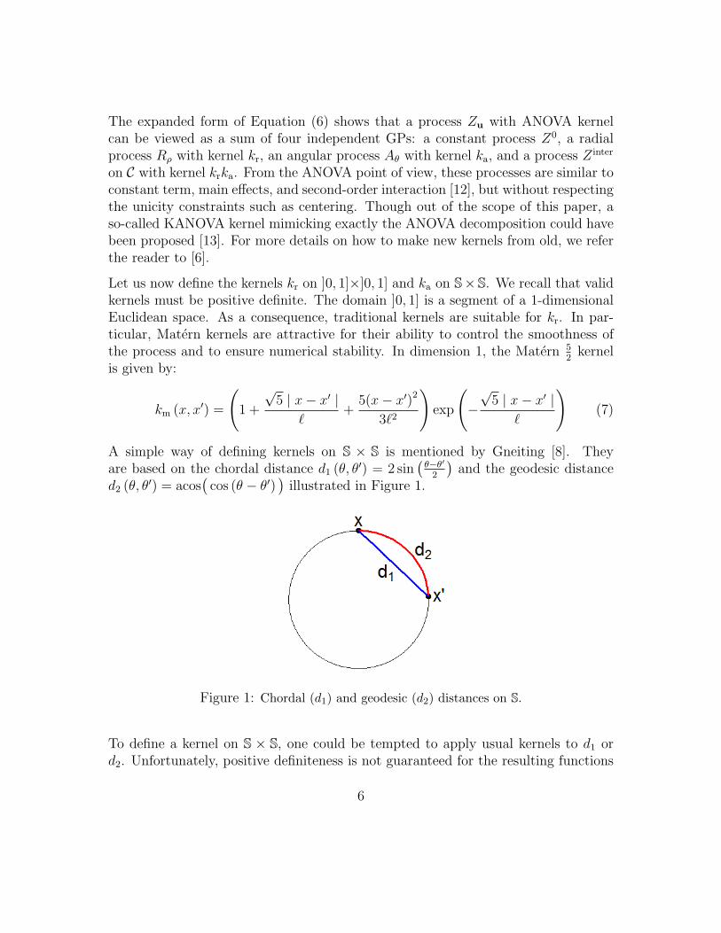
A simple way of defining kernels on S × S is mentioned by Gneiting [8]. Theyare based on the chordal distance d1 (θ, θ′) = 2 sin

(θ−θ′

2

)and the geodesic distance

d2 (θ, θ′) = acos(

cos (θ − θ′))

illustrated in Figure 1.

Figure 1: Chordal (d1) and geodesic (d2) distances on S.

To define a kernel on S × S, one could be tempted to apply usual kernels to d1 ord2. Unfortunately, positive definiteness is not guaranteed for the resulting functions

6

when d2 is used. As a counter-example, if the Gaussian kernel is chosen for ka, thenka ◦ d2 is not positive definite ([8], Th. 8). Two sufficient conditions are given in [8] :

(i). If h : [0,∞)→ R is a kernel, then h ◦ d1 is a kernel on S× S

(ii). If in addition h (t) = 0 for t ≥ π, then h ◦ d2 is a kernel on S× S

Kernels satisfying (i) were initially proposed by Yadrenko in 1983 [8] and are of-ten used to describe periodic functions [6]. They correspond to restrictions of 2-dimensional isotropic GPs on R2 to S. Kernels satisfying (ii) can be constructedfrom compactly supported functions on R such as the C2-Wendland function definedfor 0 ≤ t ≤ π:

Wc (t) =

(1 + τ

t

c

)(1− t

c

)τ+

, c ∈]0, π]; τ ≥ 4 (8)

For the geodesic distance, we use c = π, which is the largest possible value due tocondition (ii) above. With this choice, the covariance between two angles θ, θ′ is zerowhen d2(θ, θ

′) = π, and strictly positive for d2(θ, θ′) < π. The same interpretation

is possible for the chordal distance with c = 2, though it is not necessary to use acompactly supported function in that case. From now on, we will use the Wendlandfunction in both cases, resulting in the two following kernels on S× S:

kchord(θ, θ′) = W2(d1(θ, θ′)), (9)

kgeo(θ, θ′) = Wπ(d2(θ, θ

′)), (10)

and the corresponding GPs will be denoted polar GP (chordal) and polar GP (geodesic).

GP simulations on the unit disk

In order to have a first contact with polar GPs, it is useful to draw simulated sur-faces. For the sake of simplicity, we propose to focus on the ANOVA combinations.We consider a Cartesian GP and the two polar GPs (chordal, geodesic) defined inEquations (9), (10). Their expressions are written below, including variance factorss2, α2

1, α22:

(a) k (x,x′) = s2(

1 + α21 km

(x, x′

))(1 + α2

2 km (y, y′))

(b) k (x,x′) = s2(

1 + α21 km

(ρ, ρ′

))(1 + α2

2 kchord (θ, θ′))

7

(c) k (x,x′) = s2(

1 + α21 km

(ρ, ρ′

))(1 + α2

2 kgeo (θ, θ′))

Simulation results are displayed in Figure 2. We can see that with polar GPs, thesimulated surface exhibits radial and angular patterns around the center of the disk.Such kernels may thus be suitable to describe physical phenomena involving sucheffects. Figure 3 shows via Kriging standard deviation how model uncertainty variesover D, given a design of 17 points. Two striking differences are visible, especiallybetween the Cartesian GP and the polar GP (geodesic), about uncertainty at thecenter of the disk, and uncertainty regions at the vicinity of design points. On onehand, the neighborhoods produced by the Cartesian GP look lie elliptical regions atany location of the circular domain. On the other hand, those produced by the polarGP (geodesic) look like pie chart sectors oriented towards the center of the disk,which plays a particular role. This is also true for the polar GP (chordal), thoughless pronounced.

Cartesian GP Polar GP (chordal) Polar GP (geodesic)

Figure 2: Simulations of Cartesian and polar GPs with kernels (a)-(c).

8

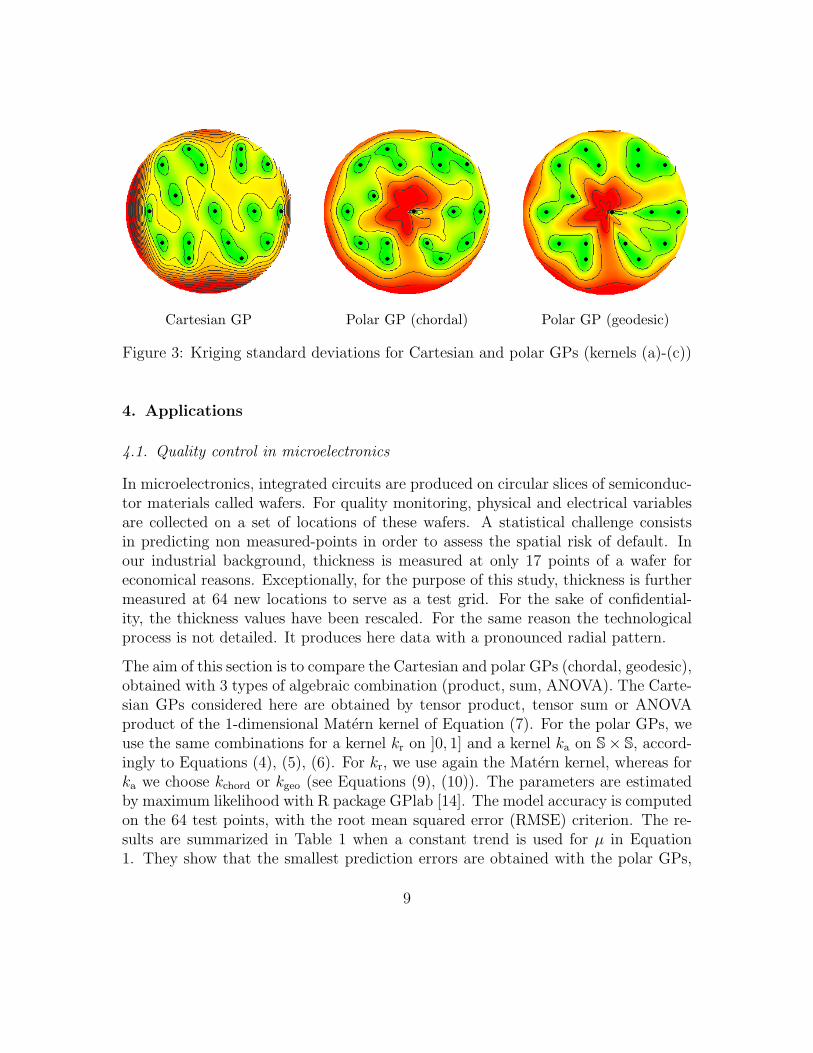
Cartesian GP Polar GP (chordal) Polar GP (geodesic)

Figure 3: Kriging standard deviations for Cartesian and polar GPs (kernels (a)-(c))

4. Applications

4.1. Quality control in microelectronics

In microelectronics, integrated circuits are produced on circular slices of semiconduc-tor materials called wafers. For quality monitoring, physical and electrical variablesare collected on a set of locations of these wafers. A statistical challenge consistsin predicting non measured-points in order to assess the spatial risk of default. Inour industrial background, thickness is measured at only 17 points of a wafer foreconomical reasons. Exceptionally, for the purpose of this study, thickness is furthermeasured at 64 new locations to serve as a test grid. For the sake of confidential-ity, the thickness values have been rescaled. For the same reason the technologicalprocess is not detailed. It produces here data with a pronounced radial pattern.

The aim of this section is to compare the Cartesian and polar GPs (chordal, geodesic),obtained with 3 types of algebraic combination (product, sum, ANOVA). The Carte-sian GPs considered here are obtained by tensor product, tensor sum or ANOVAproduct of the 1-dimensional Matern kernel of Equation (7). For the polar GPs, weuse the same combinations for a kernel kr on ]0, 1] and a kernel ka on S× S, accord-ingly to Equations (4), (5), (6). For kr, we use again the Matern kernel, whereas forka we choose kchord or kgeo (see Equations (9), (10)). The parameters are estimatedby maximum likelihood with R package GPlab [14]. The model accuracy is computedon the 64 test points, with the root mean squared error (RMSE) criterion. The re-sults are summarized in Table 1 when a constant trend is used for µ in Equation1. They show that the smallest prediction errors are obtained with the polar GPs,

9

corresponding to gains around 20% compared to the Cartesian GP. Adding Zernikepolynomials as a trend slightly improves the result for the Cartesian GP, but the un-trended polar GPs still outperform with a gain of 15%. Actually the trend capturesthe main part of the phenomenon and the GP part has then a minor effect: resultsare the same as for a pure linear model based on Zernike polynomials of order 2.

In order to further analyze the results, we select for each GP type the kernel corre-sponding to the best combination, repaired by an asterisk in Table 1. The predictionsurfaces obtained with these 3 kernels are shown on Figure 5. All the GPs succeed inrecovering the radial pattern of the dataset, visible on Figure 4, middle. However, itis less faithfully identified by the Cartesian GP, though the radial property is detected

by estimation: Indeed its kernel approximately depends on(x−x′

`1

)2

+(y−y′

`2

)2

, and

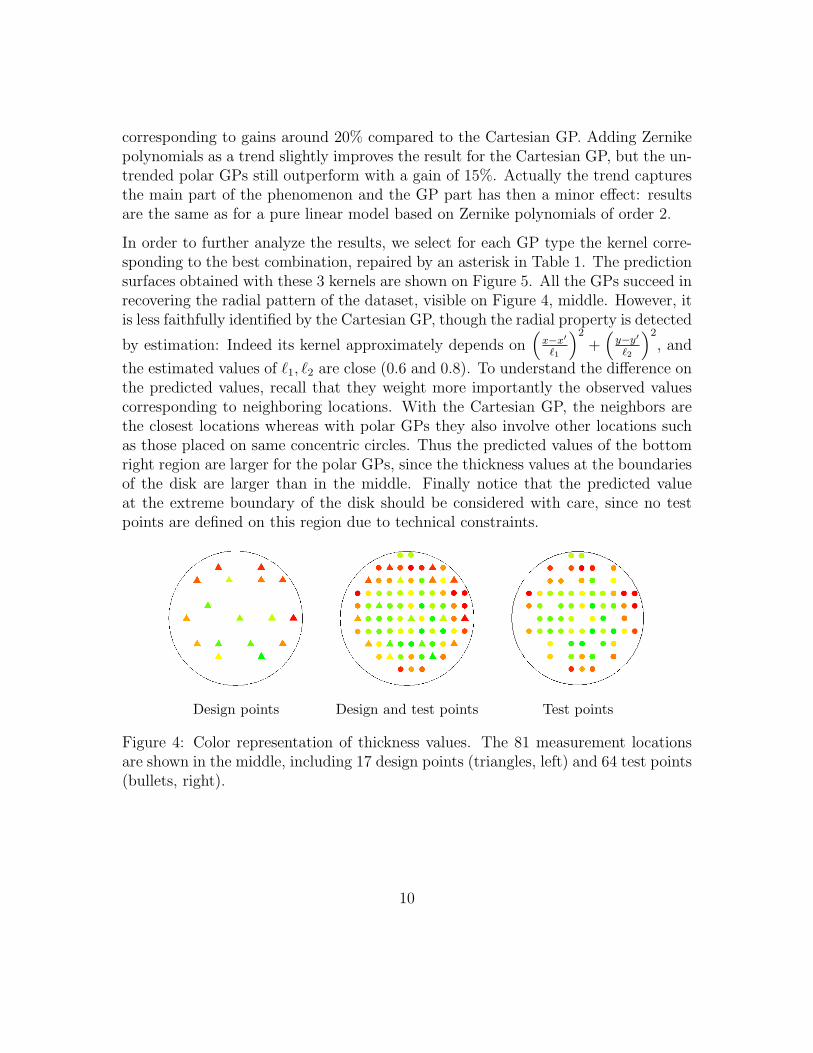
the estimated values of `1, `2 are close (0.6 and 0.8). To understand the difference onthe predicted values, recall that they weight more importantly the observed valuescorresponding to neighboring locations. With the Cartesian GP, the neighbors arethe closest locations whereas with polar GPs they also involve other locations suchas those placed on same concentric circles. Thus the predicted values of the bottomright region are larger for the polar GPs, since the thickness values at the boundariesof the disk are larger than in the middle. Finally notice that the predicted valueat the extreme boundary of the disk should be considered with care, since no testpoints are defined on this region due to technical constraints.

Design points Design and test points Test points

Figure 4: Color representation of thickness values. The 81 measurement locationsare shown in the middle, including 17 design points (triangles, left) and 64 test points(bullets, right).

10

GP type Cartesian Polar (chordal) Polar (geodesic)Kernel type kprod kadd kANOVA kprod kadd kANOVA kprod kadd kANOVA

RMSE 0.75 * 0.77 0.76 0.69 0.60 * 0.62 0.68 0.61 * 0.65

Table 1: RMSE computed on 64 test points for several GPs with a constant trend.For each GP type, the combination resulting in the smallest RMSE is marked by anasterisk. When a Zernike trend is added, the best RMSE is equal to 0.71 for all GPtypes, corresponding to the score of the linear trend only.

Zernike regression Cartesian GP Polar GP (chordal) Polar GP (geodesic)

Figure 5: Prediction surface for the best untrended GP models of Table 1. Whenadding a Zernike trend, the prediction surface is approximately the same as for a pureZernike regression represented on the left. Black bullets correspond to test points,triangles to design points.

4.2. Air pollution modelling with a directional input

The problem tackled here is a an environmental question. A greenhouse gas emittedby a known source, usually an industrial plant, is measured at a given location for airquality monitoring. In the absence of sensors, gas concentration must be predicted.For simple landscapes, analytical expressions are available based on transport anddiffusion equations. However, for complex landscapes, gas concentration is simulatedby numerical codes [15]. The input variables include the emitted flow, landscapecharacteristics and meteorological variables. Here we focus on wind speed and winddirection. In this short study, 242 simulations were carried out, 30 of which serve asdesign points and the other ones are used for tests, as illustrated in Figure 6. Thewind speed, initially given on the range [0; 12] (m.s−1), is rescaled to [0, 1]. Withthis transformation, the domain of the variables (speed, direction) is the unit disk.

The aim of this study is simply to compare the prediction accuracy of Cartesian and

11

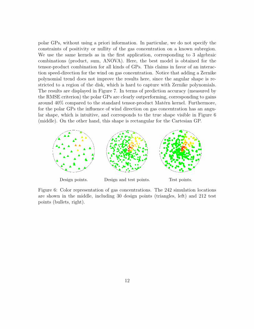
polar GPs, without using a priori information. In particular, we do not specify theconstraints of positivity or nullity of the gas concentration on a known subregion.We use the same kernels as in the first application, corresponding to 3 algebraiccombinations (product, sum, ANOVA). Here, the best model is obtained for thetensor-product combination for all kinds of GPs. This claims in favor of an interac-tion speed-direction for the wind on gas concentration. Notice that adding a Zernikepolynomial trend does not improve the results here, since the angular shape is re-stricted to a region of the disk, which is hard to capture with Zernike polynomials.The results are displayed in Figure 7. In terms of prediction accuracy (measured bythe RMSE criterion) the polar GPs are clearly outperforming, corresponding to gainsaround 40% compared to the standard tensor-product Matern kernel. Furthermore,for the polar GPs the influence of wind direction on gas concentration has an angu-lar shape, which is intuitive, and corresponds to the true shape visible in Figure 6(middle). On the other hand, this shape is rectangular for the Cartesian GP.

Design points. Design and test points. Test points.

Figure 6: Color representation of gas concentrations. The 242 simulation locationsare shown in the middle, including 30 design points (triangles, left) and 212 testpoints (bullets, right).

12

Cartesian GPRMSE = 0.61

Polar GP (chordal)RMSE = 0.38

Polar GP (geodesic)RMSE = 0.37

Figure 7: Estimated gas concentrations according to wind speed (ρ) and direction(θ), for untrended Cartesian and polar GPs. Adding a Zernike polynomial trend doesnot improve the results. Triangles correspond to design points.

5. Design of experiments on the disk

5.1. Optimal designs for Zernike polynomials and spirals

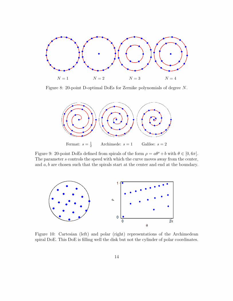
Among the DoEs that are specific to the disk, there are optimal designs for Zernikepolynomials. The D-optimal designs were investigated by [2] and were found to becontained in few concentric circles, as illustrated in Figure 8.Spirals, hereafter denoted spiral DoEs, are used in various industrial settings: Mi-croelectronics, optics, microbiology, etc. They allow to control the density of thedesign [16]. Some of them are represented in Figure 9, corresponding to the equationρ = aθp + b.

Some issues arise from these two classes of DoEs. D-optimal DoEs for regressionmodels are not robust to departures from the assumed shapes [17], and do not fillthe space, a property usually required in the framework of GP modelling for capturingpotential non-linearities. Poor space-filling properties are also visible for spirals in thespace (ρ, θ) of polar coordinates, as shown in Figure 10, though they may correctlyfill the disk.

13

N = 1 N = 2 N = 3 N = 4

Figure 8: 20-point D-optimal DoEs for Zernike polynomials of degree N .

Fermat: s = 12 Archimede: s = 1 Galilee: s = 2

Figure 9: 20-point DoEs defined from spirals of the form ρ = aθs+ b with θ ∈ [0, 6π].The parameter s controls the speed with which the curve moves away from the center,and a, b are chosen such that the spirals start at the center and end at the boundary.

Figure 10: Cartesian (left) and polar (right) representations of the Archimedeanspiral DoE. This DoE is filling well the disk but not the cylinder of polar coordinates.

14

5.2. Maximin Latin hypercubes for polar coordinates.

For metamodelling a potentially complex phenomenon, two main properties are ex-pected from a good DoE: Space-filling, in order to capture non-linearities, and uni-formity of the marginal distributions, to avoid redundancies in projection. Amongthe indicators used to assess space-fillingness, the maximin criterion [18] is a commonchoice. In addition, Latin hypercube designs (LHD, [10]) provide good projectionproperties onto marginal dimensions. Thus, maximin LHDs are often proposed asinitial DoEs. However such designs cannot be directly used in polar coordinates, dueto the non-Euclidian structure of C. To adapt their construction is the aim of thissection.

Let us first recall the construction of a maximin LHD over the hypercubic domain[0, 1]2. Given a design X =

(x(1), . . . ,x(n)

)of elements of [0, 1]2, we denote ΦMn (X)

the so-called maximin criterion, giving the minimal distance among design points:

ΦMn (X) = mini 6=j

(‖ x(i) − x(j) ‖

)(11)

A maximin DoE is a design that maximizes ΦMn. However, ΦMn is hard to optimizeand [19] proposed a regularized version φp, more suitable for optimization:

φp (X) =

( ∑1≤i<j≤n

‖ x(i) − x(j) ‖−p) 1

p

(12)

For p → ∞, maximizing ΦMn is equivalent to minimizing φp. Following [19, 20], wewill use p = 50. In softwares, the algorithms used for optimization are often basedon simulated annealing or evolutionary strategies (see e.g. [21]).

Now let us consider the cylinder C of polar coordinates. The construction of a Latinhypercube on C is identical for an hypercubic domain, by considering discretizationsof [0, 1] and S. However, the maximin criterion must be adapted to a valid distanceon C, ensuring that ‖ u−u′ ‖= 0 for u = (ρ, θ) and u′ = (ρ, θ′), with θ = θ′ (mod 2π).In particular the Euclidian distance is not further valid, since it does not see that thepoints (ρ, 0) and (ρ, 2π) are the same in C. Valid distances on C can be obtained bycombining distances on ]0, 1] and S. We propose to consider the following distance:

‖ x− x′ ‖Polar=

√(ρ− ρ′)2 +

(d2 (θ, θ′)

π

)2

(13)

The factor 1π

rescales d2 to [0, 1] in order to weight equivalently radius and angle.

15

From now on we will denote ΦPolar (resp. ΦCartesian) the Φp criteria computed with‖ . ‖Polar (resp. ‖ . ‖2). Minimizing ΦPolar leads to a maximin LHD according to(ρ, θ). A 20-point maximin LHD is displayed in Figure 11, where the cylinder isrepresented as a 2-dimensional map. As expected it is well filling the space of polarcoordinates. Though it looks similar to a maximin LHD obtained in an hypercubicdomain with the usual Euclidian distance, the difference is visible on the left andright boundaries which correspond to the same points in C: the design points nearthe left and right boundaries are also spread out from each other.

Figure 11: Cartesian (left) and polar (right) representations of a 20-point maximinLHD. The design is well-filling the cylinder C of polar coordinates, displayed as a 2-dimensional map: In particular, the design points near the left and right boundariesare also spread out from each other.

The LHDs constructed on C are recommended when the studied phenomenon has aphysical interpretation with respect to polar coordinates. First, if the phenomenonis purely radial (resp. angular), the Latin hypercube structure ensures that all thedesign radius (resp. angles) values are different, so that no information is lost by pro-jection. Furthermore, the maximin property helps in capturing non-linearities withrespect to ρ and θ. However, when no a priori information about the phenomenonis known, the maximin LHDs on C may be inappropriate, due to non-uniform fillingthat they produce on D, as visible in Figure 11.

Though it is not possible to optimize simultaneously maximin criteria based on dis-tances in Cartesian and polar coordinates, a multi-criteria approach could have beeninvestigated. In this paper, as a first study, we focus on a simple transformation ofa maximin LHS on C which helps improving space-fillingness on D while preservingthe Latin hypercube structure on C. This is done by applying the transform ρ 7→ √ρ,based on the well-known fact that if R is a uniform random variable on [0, 1] and T is

16

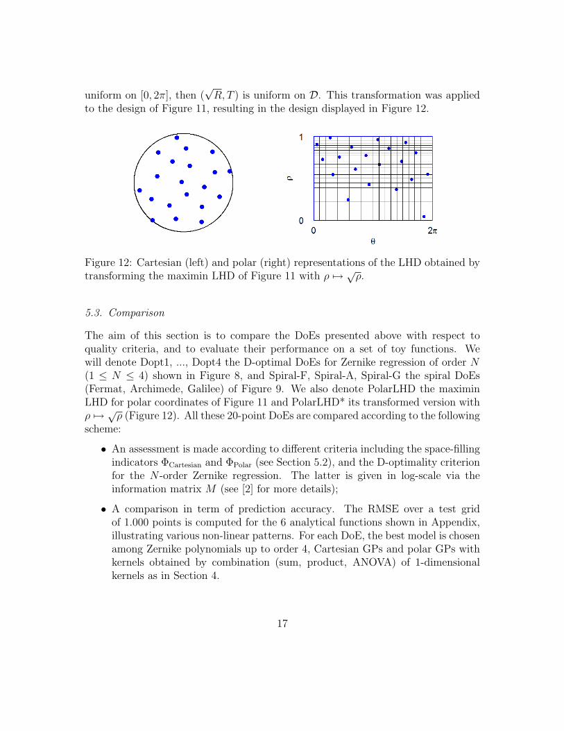
uniform on [0, 2π], then (√R, T ) is uniform on D. This transformation was applied

to the design of Figure 11, resulting in the design displayed in Figure 12.

Figure 12: Cartesian (left) and polar (right) representations of the LHD obtained bytransforming the maximin LHD of Figure 11 with ρ 7→ √ρ.

5.3. Comparison

The aim of this section is to compare the DoEs presented above with respect toquality criteria, and to evaluate their performance on a set of toy functions. Wewill denote Dopt1, ..., Dopt4 the D-optimal DoEs for Zernike regression of order N(1 ≤ N ≤ 4) shown in Figure 8, and Spiral-F, Spiral-A, Spiral-G the spiral DoEs(Fermat, Archimede, Galilee) of Figure 9. We also denote PolarLHD the maximinLHD for polar coordinates of Figure 11 and PolarLHD* its transformed version withρ 7→ √ρ (Figure 12). All these 20-point DoEs are compared according to the followingscheme:

• An assessment is made according to different criteria including the space-fillingindicators ΦCartesian and ΦPolar (see Section 5.2), and the D-optimality criterionfor the N -order Zernike regression. The latter is given in log-scale via theinformation matrix M (see [2] for more details);

• A comparison in term of prediction accuracy. The RMSE over a test gridof 1.000 points is computed for the 6 analytical functions shown in Appendix,illustrating various non-linear patterns. For each DoE, the best model is chosenamong Zernike polynomials up to order 4, Cartesian GPs and polar GPs withkernels obtained by combination (sum, product, ANOVA) of 1-dimensionalkernels as in Section 4.

17

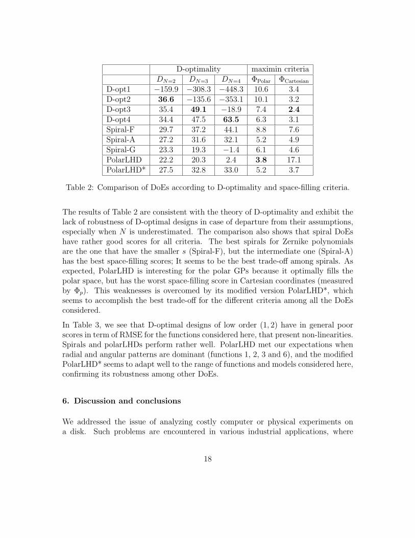
D-optimality maximin criteriaDN=2 DN=3 DN=4 ΦPolar ΦCartesian

D-opt1 −159.9 −308.3 −448.3 10.6 3.4D-opt2 36.6 −135.6 −353.1 10.1 3.2D-opt3 35.4 49.1 −18.9 7.4 2.4D-opt4 34.4 47.5 63.5 6.3 3.1Spiral-F 29.7 37.2 44.1 8.8 7.6Spiral-A 27.2 31.6 32.1 5.2 4.9Spiral-G 23.3 19.3 −1.4 6.1 4.6PolarLHD 22.2 20.3 2.4 3.8 17.1PolarLHD* 27.5 32.8 33.0 5.2 3.7

Table 2: Comparison of DoEs according to D-optimality and space-filling criteria.

The results of Table 2 are consistent with the theory of D-optimality and exhibit thelack of robustness of D-optimal designs in case of departure from their assumptions,especially when N is underestimated. The comparison also shows that spiral DoEshave rather good scores for all criteria. The best spirals for Zernike polynomialsare the one that have the smaller s (Spiral-F), but the intermediate one (Spiral-A)has the best space-filling scores; It seems to be the best trade-off among spirals. Asexpected, PolarLHD is interesting for the polar GPs because it optimally fills thepolar space, but has the worst space-filling score in Cartesian coordinates (measuredby Φp). This weaknesses is overcomed by its modified version PolarLHD*, whichseems to accomplish the best trade-off for the different criteria among all the DoEsconsidered.

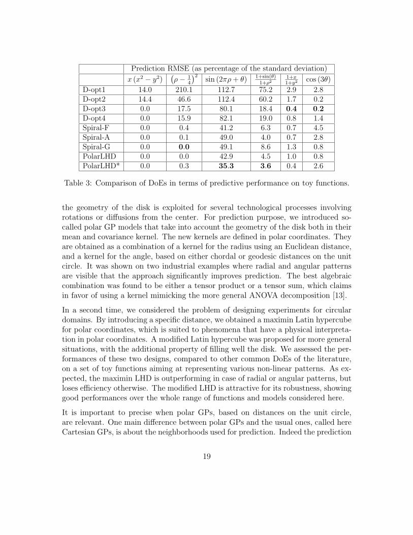
In Table 3, we see that D-optimal designs of low order (1, 2) have in general poorscores in term of RMSE for the functions considered here, that present non-linearities.Spirals and polarLHDs perform rather well. PolarLHD met our expectations whenradial and angular patterns are dominant (functions 1, 2, 3 and 6), and the modifiedPolarLHD* seems to adapt well to the range of functions and models considered here,confirming its robustness among other DoEs.

6. Discussion and conclusions

We addressed the issue of analyzing costly computer or physical experiments ona disk. Such problems are encountered in various industrial applications, where

18

Prediction RMSE (as percentage of the standard deviation)

x (x2 − y2)(ρ− 1

4

)2sin (2πρ+ θ) 1+sin(θ)

1+ρ21+x1+y2

cos (3θ)

D-opt1 14.0 210.1 112.7 75.2 2.9 2.8D-opt2 14.4 46.6 112.4 60.2 1.7 0.2D-opt3 0.0 17.5 80.1 18.4 0.4 0.2D-opt4 0.0 15.9 82.1 19.0 0.8 1.4Spiral-F 0.0 0.4 41.2 6.3 0.7 4.5Spiral-A 0.0 0.1 49.0 4.0 0.7 2.8Spiral-G 0.0 0.0 49.1 8.6 1.3 0.8PolarLHD 0.0 0.0 42.9 4.5 1.0 0.8PolarLHD* 0.0 0.3 35.3 3.6 0.4 2.6

Table 3: Comparison of DoEs in terms of predictive performance on toy functions.

the geometry of the disk is exploited for several technological processes involvingrotations or diffusions from the center. For prediction purpose, we introduced so-called polar GP models that take into account the geometry of the disk both in theirmean and covariance kernel. The new kernels are defined in polar coordinates. Theyare obtained as a combination of a kernel for the radius using an Euclidean distance,and a kernel for the angle, based on either chordal or geodesic distances on the unitcircle. It was shown on two industrial examples where radial and angular patternsare visible that the approach significantly improves prediction. The best algebraiccombination was found to be either a tensor product or a tensor sum, which claimsin favor of using a kernel mimicking the more general ANOVA decomposition [13].

In a second time, we considered the problem of designing experiments for circulardomains. By introducing a specific distance, we obtained a maximin Latin hypercubefor polar coordinates, which is suited to phenomena that have a physical interpreta-tion in polar coordinates. A modified Latin hypercube was proposed for more generalsituations, with the additional property of filling well the disk. We assessed the per-formances of these two designs, compared to other common DoEs of the literature,on a set of toy functions aiming at representing various non-linear patterns. As ex-pected, the maximin LHD is outperforming in case of radial or angular patterns, butloses efficiency otherwise. The modified LHD is attractive for its robustness, showinggood performances over the whole range of functions and models considered here.

It is important to precise when polar GPs, based on distances on the unit circle,are relevant. One main difference between polar GPs and the usual ones, called hereCartesian GPs, is about the neighborhoods used for prediction. Indeed the prediction

19

of a GP model is weighting more importantly the observed values corresponding toneighboring locations. For Cartesian GPs, the neighborhoods of a given locationcorrespond to elliptical regions, whereas for geodesic (or chordal) distance, they looklike pie chart sectors. This explains why polar GPs give more accurate predictionswhen there are radial or angular patterns, as may happen for technological processesthat involve a rotation or a diffusion from the center. In other situations, involvingfor instance translations, Cartesian GPs may give better results. These two casesmight correspond to the“two clusters of profiles over a circular grid”mentioned by [3]without any additional information about their origin. A knowledge of the processor historical data may help choosing which kernel is appropriate. In any case, thereremains a lot of degrees of freedom about a GP model definition, concerning at leastthe trend shape or the different kernels corresponding to a given distance. To addressthis problem, aggregation techniques may be a solution.

The discussion above concerning the model choice raises several questions about de-sign of experiments. The study presented in this paper shows the possibility to adaptexisting criteria to new distances. In the situations where there is no informationabout processing, choosing a distance may be difficult, and there is a need for build-ing DoEs that can be suitable for any distance. In such case, a solution would be toconsider a multi-criteria approach, for instance by aggregating the maximin criteriain Cartesian and polar coordinates. On the other hand, if a specific kernel is justified,then IMSE-optimal designs could be computed with respect to this kernel.

20

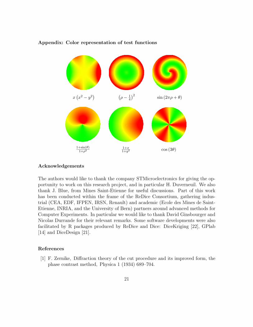
Appendix: Color representation of test functions

x(x2 − y2

) (ρ− 1

4

)2 sin (2πρ+ θ)

1+sin(θ)1+ρ2

1+x1+y2 cos (3θ)

Acknowledgements

The authors would like to thank the company STMicroelectronics for giving the op-portunity to work on this research project, and in particular H. Duverneuil. We alsothank J. Blue, from Mines Saint-Etienne for useful discussions. Part of this workhas been conducted within the frame of the ReDice Consortium, gathering indus-trial (CEA, EDF, IFPEN, IRSN, Renault) and academic (Ecole des Mines de Saint-Etienne, INRIA, and the University of Bern) partners around advanced methods forComputer Experiments. In particular we would like to thank David Ginsbourger andNicolas Durrande for their relevant remarks. Some software developments were alsofacilitated by R packages produced by ReDice and Dice: DiceKriging [22], GPlab[14] and DiceDesign [21].

References

[1] F. Zernike, Diffraction theory of the cut procedure and its improved form, thephase contrast method, Physica 1 (1934) 689–704.

21

[2] H. Dette, V. Melas, A. Pepelyshev, Optimal Designs for Statistical Analysiswith Zernike Polynomials, Technical report: Sonderforschungsbereich Komplex-itatsreduktion in Multivariaten Datenstrukturen, Univ., SFB 475, 2006.

[3] G. Pistone, G. Vicario, Kriging prediction from a circular grid: application towafer diffusion, Applied Stochastic Models in Business and Industry 29 (2013)350–361.

[4] K. V. Mardia, P. E. Jupp, Directional Statistics, Wiley, 2000.

[5] N. Fisher, Statistical Analysis of Circular Data, Statistical Analysis of CircularData, Cambridge University Press, 1995.

[6] C. Rasmussen, C. Williams, Gaussian Processes for Machine Learning, The MITPress, 2006.

[7] G. Jona-Lasinio, A. Gelfand, M. Jona-Lasinio, Spatial Analysis of Wave Direc-tion Data using Wrapped Gaussian Processes, The Annals of Applied Statistics6 (2012) 1478–1498.

[8] T. Gneiting, Strictly and non-strictly positive definite functions on spheres,Bernoulli 19 (2013) 1327–1349.

[9] E. del Castillo, B. M. Colosimo, S. Tajbakhsh, Geodesic Gaussian Processes forthe Parametric Reconstruction of a Free-Form Surface, to appear in Techno-metrics (2015).

[10] M. D. McKay, R. J. Beckman, W. J. Conover, A comparison of three methodsfor selecting values of input variables in the analysis of output from a computercode, Technometrics 21 (1979) 239–245.

[11] G. Matheron, Principles of geostatistics, volume 58, Society of Economic Geol-ogists, 1963.

[12] N. Durrande, D. Ginsbourger, O. Roustant, L. Carraro, ANOVA kernels andRKHS of zero mean functions for model-based sensitivity analysis, Journal ofMultivariate Analysis 115 (2013) 57–67.

[13] D. Ginsbourger, O. Roustant, D. Schuhmacher, N. Durrande, N. Lenz, OnANOVA decompositions of kernels and Gaussian random field paths, ArXive-prints (2014).

22

[14] Y. Deville, D. Ginsbourger, N. Roustant, O. Contributors: Durrande, GPlab:Laboratory for DiceKriging, 2015. R package version 0.1.0.

[15] M. Batton-Hubert, M. Binois, E. Padonou, Inverse modeling to estimatemethane surface emission with optimization and reduced models: applicationof waste landfill plants, in: 13th Annual Conference of the European Networkfor Business and Industrial, Ankara, Turkey.

[16] R. Navarro, J. Arines, Complete Modal Representation with Discrete ZernikePolynomials - Critical Sampling in Non Redundant Grids, INTECH Open AccessPublisher, 2011.

[17] P. Huber, Robust Statistics, Wiley Series in Probability and Statistics, Wiley-Interscience, 1981.

[18] M. Morris, Gaussian surrogates for computer models with time-varying inputsand outputs, Technometrics 54 (2012) 42–50.

[19] M. Morris, T. Mitchell, Exploratory designs for computational experiments,Journal of Statistical Planning and Inference 43 (1995) 381–402.

[20] G. Damblin, M. Couplet, B. Iooss, Numerical studies of space filling designs:optimization of Latin hypercube samples and subprojection properties, Journalof Simulation 7 (2013) 276–289.

[21] J. Franco, D. Dupuy, O. Roustant, G. Damblin, B. Iooss., DiceDesign: Designsof Computer Experiments, 2014. R package version 1.6.

[22] O. Roustant, D. Ginsbourger, Y. Deville, DiceKriging, DiceOptim: Two R pack-ages for the analysis of computer experiments by kriging-based metamodelingand optimization, Journal of Statistical Software 51 (2012) 1–55.

23