point value multiscale algorithms for 2d compressible flowsgchiavassa/sisc.pdf · point value...

POINT VALUE MULTISCALE ALGORITHMS FOR 2DCOMPRESSIBLE FLOWS!

GUILLAUME CHIAVASSA† AND ROSA DONAT†

SIAM J. SCI. COMPUT. c" 2001 Society for Industrial and Applied MathematicsVol. 23, No. 3, pp. 805–823

Abstract. The numerical simulation of physical problems modeled by systems of conservationlaws is di!cult due to the presence of discontinuities in the solution. High-order shock capturingschemes combine sharp numerical profiles at discontinuities with a highly accurate approximation insmooth regions, but usually their computational cost is quite large.

Following the idea of A. Harten [Comm. Pure Appl. Math., 48 (1995), pp. 1305–1342] and Bihariand Harten [SIAM J. Sci. Comput., 18 (1997), pp. 315–354], we present in this paper a method toreduce the execution time of such simulations. It is based on a point value multiresolution transformthat is used to detect regions with singularities. In these regions, an expensive high-resolution shockcapturing scheme is applied to compute the numerical flux at cell interfaces. In smooth regions acheap polynomial interpolation is used to deduce the value of the numerical divergence from valuespreviously obtained on lower resolution scales.

This method is applied to solve the two-dimensional compressible Euler equations for two classicalconfigurations. The results are analyzed in terms of quality and e!ciency.

Key words. conservation laws, multiresolution, shock capturing schemes

AMS subject classifications. 65M06, 65D05, 35L65

PII. S1064827599363988

1. Introduction. The computation of solutions to hyperbolic systems of conser-vation laws has been a very active field of research for the last 20 to 30 years and, as aresult, there are now a variety of methods that are able to compute accurate numericalapproximations to the physically relevant solution. The latest addition to the pool ofnumerical methods for hyperbolic conservation laws are the modern high-resolutionshock capturing (HRSC) schemes. These schemes succeed in computing highly ac-curate numerical solutions, typically second- or third-order in smooth regions, whilemaintaining sharp, oscillation-free numerical profiles at discontinuities.

State-of-the-art shock capturing schemes usually perform a “delicate art-craft” onthe computation of the numerical flux functions. A typical computation involves atleast one eigenvalue-eigenvector decomposition of the Jacobian matrix of the system,as well as the approximation of the values of the numerical solution at both sides ofeach cell interface, obtained via some appropriately chosen approximating functions.The numerical result is very often spectacular in terms of resolution power, but thecomputational e!ort also tends to be quite spectacular.

Without doubt, the computational speed of the latest personal computers andworkstations has made it possible for an increasing number of researchers to becomeinterested in HRSC methods and, as a result, HRSC methods are now being testedin a variety of physical scenarios that involve hyperbolic systems of conservation laws(see, e.g., [7, 10, 19] and references therein).

When the underlying grid is uniform, the implementation of most of these shockcapturing schemes is quite straightforward and numerical simulations on uniform grids

!Received by the editors November 16, 1999; accepted for publication (in revised form) October30, 2000; published electronically August 15, 2001. This work was supported in part by TMRResearch Network contract FMRX-CT98-0184 and by Spanish DGICYT grant PB97-1402.

http://www.siam.org/journals/sisc/23-3/36398.html†Departamento de Matematica Aplicada, Universidad de Valencia, 46100 Burjassot (Valencia),

Spain ([email protected], [email protected]).

805

806 GUILLAUME CHIAVASSA AND ROSA DONAT

are routinely used to investigate the behavior of the di!erent HRSC schemes in use,and also their limitations. It is known that some HRSC schemes can produce ananomalous behavior in certain situations; a catalog of numerical pathologies encoun-tered in gas dynamics simulations can be found in [20], where it is observed that someof these pathologies appear only when very fine meshes are used.

When using very fine uniform grids, in which the basic code structure of an HRSCscheme is relatively simple, we find that the computational time becomes the maindrawback in the numerical simulation. For some HRSC schemes, fine mesh simulationsin two dimensions are out of reach simply because they cost too much. The numericalflux evaluations are too expensive, and the computational time is measured by days ormonths on a personal computer. As an example we notice that a typical computationof a two-dimensional (2D) jet configuration in [19] is 10 to 50 days on an HP710 or 1to 5 days on an Origin 2000 with 64 processors.

It is well known, however, that the heavy-duty flux computations are needed onlybecause nonsmooth structures may develop spontaneously in the solution of a hy-perbolic system of conservation laws and evolve in time, and this basic observationhas lead researchers to the development of a number of techniques that aim at re-ducing the computational e!ort associated to these simulations. Among these, shocktracking and adaptive mesh refinement (AMR) techniques (often combined with oneanother) are very e!ective at obtaining high-resolution numerical approximations, butthe computational e!ort is transferred to the programming and the data structure ofthe code.

Starting with the pioneering work of Harten [14], a di!erent multilevel strategyaiming to reduce the computational e!ort associated to high-cost HRSC methodsentered the scene. The key observation is that the information contained in a mul-tiscale decomposition of the numerical approximation can be used to determine itslocal regularity (smoothness). At discontinuities or steep gradients, it is imperativeto use a numerical flux function that models correctly the physics of the problem, butin smoothness regions the costly exact value of an HRSC numerical flux can be re-placed by an equally accurate approximation obtained by much less expensive means.The multiscale decomposition of the numerical solution can then be used as a toolto decide in which regions a sophisticated evaluation of the numerical flux function istruly needed. In smoothness regions, Harten proposes [14] to evaluate the numericalflux function of the HRSC scheme only on a coarse grid and then use these values tocompute the fluxes on the finest grid using an inexpensive polynomial interpolationprocess in a multilevel fashion.

Harten’s approach can be viewed, in a way, as an AMR procedure, in which gridsof di!erent resolutions are considered in the numerical simulation, but in reality it isfar from being an AMR technique. The di!erent grids are used only to analyze thesmoothness of the numerical solution. The numerical values on the highest-resolutiongrid need to be always available, because the computation of the numerical fluxes withthe HRSC scheme, when needed, use directly the finest-grid values. This is clearly adisadvantage with respect to the memory savings that an AMR technique can o!erin certain situations. On the other hand, using the values of the numerical solution inthe direct computation has some nice features. First, it avoids the use of complicateddata structures, which is very useful when one is trying to incorporate the algorithminto an existing code. Second, the availability of the numerical solution on the finestgrid guarantees that the “delicate art-craft” involved in the direct evaluation of thenumerical fluxes (via a sophisticated HRSC scheme) is performed adequately.

MULTISCALE ALGORITHMS FOR COMPRESSIBLE FLOWS 807

When memory requirements do not impose a severe restriction (as it often hap-pens in many 2D, as well as in some three-dimensional (3D), computations), thetechniques proposed in [14, 5, 22, 1] and in this paper can help to reduce the largerunning times associated to numerical simulations with HRSC schemes. We viewHarten’s approach as an acceleration tool, which can be incorporated in a straight-forward manner into an existing code.

The novelty of our approach with respect to the multilevel strategies described in[14, 5, 22, 1] lies in the multiresolution transform used to analyze the smoothness ofthe numerical solution. We use the interpolatory framework, while in the referencesmentioned above the cell-average framework is used. In addition, our implementationincorporates several features that improve the e"ciency of the algorithm (see section3.3), while maintaining the quality of the numerical approximation.

The rest of the paper is organized as follows: In section 2, we briefly describethe essential features of the HRSC schemes we shall employ in our simulations. Insection 3 we describe the interpolatory framework for multiresolution and its role inour multilevel strategy, as well as some implementation details. Section 4 examinesthe accumulation of error in the multilevel simulation. In section 5 we perform a seriesof numerical experiments and analyze the results in terms of quality, i.e., closeness tothe reference simulation, and e!ciency, i.e., time savings of the multilevel simulationswith respect to the reference simulation. Finally, some conclusions are drawn insection 6.

2. Shock capturing schemes for 2D systems of conservation laws. Letus consider a 2D system of hyperbolic conservation laws:

!t"U + "f("U)x + "g("U)y = "0,(2.1)

where "U is the vector of conserved quantities. We shall consider discretizations ofthis system on a Cartesian grid G0 = {(xi = i#x, yj = j#y), i = 0, . . . , Nx j =0, . . . , Ny} that follow a semidiscrete formulation,

d"Uij

dt+ D("U)ij = 0,(2.2)

with the numerical divergence D("U)ij in conservation form, i.e.,

D("U)ij ="Fi+1/2,j ! "Fi#1/2,j

#x+"Gi,j+1/2 ! "Gi,j#1/2

#y.(2.3)

One typically has "Fi+1/2,j = "F ("Ui#k,j , . . . , "Ui+m,j), "Gi,j+1/2 = "G("Ui,j#k, . . . , "Ui,j+m),

where "F ("w1, . . . , "wk+m) and "G("w1, . . . , "wk+m) are consistent numerical flux functions,which are the trademark of the scheme.

In this paper we shall use two numerical flux formulae, which are significantlydi!erent in terms of computational e!ort:

– The essentially nonoscillatory (ENO) method of order 3 (ENO-3 henceforth)from [21], which uses the nonlinear piecewise parabolic ENO reconstructionprocedure to achieve high accuracy in space.

– Marquina’s scheme from [8] together with the piecewise hyperbolic method(PHM) [18] to obtain high accuracy in space (M-PHM henceforth).

In both cases, the reconstruction procedure (piecewise parabolic ENO or piecewisehyperbolic) is applied directly on the fluxes, as specified by Shu and Osher in [21].


The ENO-3 scheme uses Roe’s linearization and involves one Jacobian evaluationper cell interface, while M-PHM uses a flux-splitting technique in the flux computationthat requires two Jacobian evaluations per cell interface. Although M-PHM is moreexpensive than ENO-3, it has been shown in [8, 12, 9] that it is a pretty robust schemethat, in addition, avoids (or reduces) certain numerical pathologies associated to theRoe solver.

In both cases, a third-order fully discrete scheme is obtained by applying a TVDRunge–Kutta method for the time evolution as proposed in [21].

3. The multilevel algorithm. As explained in the introduction, the goal of themultilevel method is to decrease the cpu time associated to the underlying scheme byreducing the number of expensive flux evaluations. To understand the basic mecha-nism by which this goal is achieved, let us consider, for the sake of simplicity, Euler’smethod applied to (2.2), i.e.,

"Un+1ij = "Un

ij ! #t D("U)nij .(3.1)

If both Un and Un+1 are smooth around (xi, yj) at time tn, then (3.1) implies thatthe numerical divergence is also smooth at that location; thus we can, in principle,avoid using the numerical flux functions of the HRSC scheme in its computation. Onthe other hand, if a discontinuity appears during the time evolution (or when a steepgradient makes it imminent), the Riemann solver of the HRSC scheme has to be callednecessarily to compute the numerical divergence if the high-resolution properties ofthe underlying scheme are to be maintained.

Consequently, the most important steps in the multilevel algorithm concern thesmoothness analysis of Un and Un+1 (observe that the latter is unknown at time n)and how this information is used in the computation of D("U).

3.1. Interpolatory multiresolution. Finite volume schemes for (2.1) producenumerical values that can be naturally interpreted as approximations to the meanvalues of the solution in each computational cell (the cell averages). Because of this,all applications of Harten’s idea known to us [14, 5, 22, 6, 1, 2, 17] have invariablyused the cell-average multiresolution framework (see [14] for definitions and details)to analyze the smoothness of the numerical approximation.

In Shu and Osher’s framework, the numerical values can be interpreted as ap-proximations to the point values of the solution. In a point value framework formultiresolution, the numerical data to be analyzed are interpreted as the values ofa function on an underlying grid; consequently, in our multilevel strategy the pointvalue multiresolution framework is used to analyze the smoothness properties of thenumerical approximation.

Multiscale decompositions within the point value framework were initially intro-duced by Harten [13] (and also independently developed by Sweldens [23]) and havebeen extensively analyzed in a series of papers [15, 3]. Here we present only a briefsummary to clarify the notation in the remainder of the paper.

One first defines a set of nested grids {Gl, l = 1, . . . , L} by

(xi, yj) " Gl #$ (x2li, y2lj) " G0.(3.2)

The values of a function v on G0 (which is considered the finest resolution level),(v0

ij)i,j , are the input data. Due to the embedding of the grids, the representation of

the function on the coarser grid Gl, its point values on Gl, is

vlij = v02li 2lj , i = 0, . . . , Nx/2l, j = 0, . . . , Ny/2l.(3.3)


To recover the representation of v on Gl#1 from the representation on Gl (the nextcoarser grid), the following procedure is used:

– A set of predicted values is first computed:

vl#1ij = vli/2 j/2 if (xi, yj) " Gl,

vl#1ij = I[(xi, yj); v

l] if (xi, yj) " Gl#1\ Gl,(3.4)

where I(.; .) denotes an rth-order polynomial interpolation.– The di!erence between the exact values (3.3), vl#1

ij , and vl#1ij is then repre-

sented by the details, or wavelet coe"cients:

dlij = vl#1ij ! vl#1

ij , (xi, yj) " Gl#1.(3.5)

Observe that dl2p,2q = 0 because of the interpolation property. Thus even-evendetail coe"cients are never computed (or stored).

– Relations (3.4) and (3.5) lead immediately to

vl#1ij = vli/2 j/2 if (xi, yj) " Gl,

vl#1ij = I[(xi, yj); v

l] + dlij if (xi, yj) " Gl#1\ Gl.(3.6)

Applying this procedure from l = 1 to L gives an equivalence between the discrete setv0 and its multiresolution representation: Mv0 = (vL, dL, . . . , d1).

Remark 3.1. In our numerical experiments we use a tensor-product interpolationprocedure of order 4 (r = 4). The corresponding formulae come from standard 2Dpolynomial interpolation; explicit details can be found, for example, in [5, section 3].

The point value framework for multiresolution is probably the simplest one, be-cause the detail coe"cients are simply interpolation errors. When the grid is uniformand the interpolation technique is constructed using a tensor product approach, it isvery simple to analyze the smoothness information contained in the interpolation er-rors, which can then be used directly as “regularity sensors” to localize the nonsmoothstructures of the solution (compare with the derivation of the regularity sensors in [5]in the 2D cell-average framework for multiresolution).

3.2. The basic strategy. As observed in [5], the original idea of a multilevelcomputation of the numerical flux function (in one dimension) described by Hartenin [14] cannot be used in a robust and general manner in two dimensions. The keypoint is then to observe that it is the numerical divergence the quantity that shouldbe adapted to the multilevel computations. For the sake of simplicity, let us consideragain the simplest ODE solver: Euler’s method. When applying it to the semidiscreteformulation (2.2), we get

"Un+1ij ! "Un

ij = !#t D("U)nij ,(3.7)

and this relation shows that a multilevel computation of the numerical divergencemust be carried out within the same framework as the sets "Un,n+1

ij . The idea to usethe numerical divergence instead of the flux for the multilevel computation was a keystep in the development of multilevel strategies in multidimensions in [5, 1]. Oncethis fact is recognized, the choice of the particular framework used to analyze thesmoothness information contained in the numerical approximation is not crucial. Wepropose to use the point value framework because of its simplicity.

As in [5], the computation of the numerical divergence D("Un) on the finest gridis carried out in a sequence of steps. First the numerical divergence is evaluated at


all points on the coarsest grid GL using the numerical flux function of the prescribedHRSC scheme. Then, for the finer grids, D is evaluated recursively, either by thesame procedure or with a cheap interpolation procedure using the values obtained onthe coarser grids. The choice depends on the regularity analysis of the approximatesolution, made with the help of its multiresolution representation.

Thus, the main ingredients of the algorithm are the following:– The multiresolution transform described in section 3.1 to obtain the wavelet

coe"cients of "Un.– A thresholding algorithm which associates to each wavelet coe"cient a boolean

flag, blij , whose value (0 or 1) will determine the choice of the procedure toevaluate D(U). The goal is to use this flag to mark out the nonsmooth regionsof both "Un and "Un+1. This is done as follows:For a given tolerance parameter $, the tolerance at level l is defined as$l = $/2l. Starting from a zero value for all blij , one applies for each de-tail coe"cient the following two tests:

if |dlij | % $l =$ bli#k j#m = 1, k,m = !2, . . . , 2,

if |dlij | % 2r+1$l and l > 1 =$ bl#12i#k 2j#m = 1, k,m = !1, 0, 1.

The first test takes into account the propagation of information (recall thatthe propagation of “real” information is limited by the CFL condition). Thesecond one aims at detecting shock formation. In a smooth region the localrate of decay of the detail coe"cients is determined by the accuracy of theinterpolation and the local regularity of the function. The second test mea-sures whether the decay rate is that of a smooth function; if this is not thecase, compression leading to shock formation might be taking place and thelocation is also flagged (see [5] for specific details on both tests).

– The multilevel evaluation of the numerical divergence.For all points (xi, yj) " GL, DL("U)ij is computed with the prescribed HRSC

scheme. Once the divergence is known on Gl, its value on Gl#1, Dl#1("U) isevaluated using the boolean flag:

If blij = 1, compute Dl#1("U)ij directly (with the HRSC method).

If blij = 0, Dl#1("U)ij = I[(xi, yj);Dl("U)].

Letting l go from L to 1 gives us the values of D("Un) on the finest grid G0.Remark 3.2. Recall that Dl#1("U)ij = D0("U)2l!1i,2l!1j , and thus the direct evalu-

ation of Dl#1("U)ij is performed by computing the numerical flux functions using the

values of "U on G0: "F ("U2l!1i#k,j , . . . , "U2l!1i+m,j) and "G("Ui,2l!1j#k, . . . , "Ui,2l!1j+m).As a consequence, the finest grid, G0, is always needed and no memory savings isobtained in comparison to the direct method (without multiresolution).

3.3. Some implementation details. In the original work of Harten [14], theflag coe"cients are obtained using a multiresolution transform for each componentof the vector "U . The thresholding algorithm is then applied to the largest resultingwavelet coe"cient, i.e., dlij = max(|dij(%)|, |dij(mx)|, |dij(my)|, |dij(E)|).

For the Euler equations of gas dynamics, the density retains all the possiblenonsmooth structures of the flow (shocks, contact discontinuities, and corners of rar-efaction waves); thus it seems appropriate to derive the flag only from the multireso-lution representation of the density, a modification that has also been implemented by


Table 3.1Cpu time in seconds for the overhead steps of the multilevel algorithm. First column for all the

components of !U , second one only for the density.

!U multiresolution " multiresolutionMR transform 0.09 0.024Maximum 0.014 –Thresholding 0.026 0.027Total 0.13 0.051

Sjogreen [22]. In our experiments, no significant di!erences are noted in the qualityof the numerical results obtained by computing the flag from the density only; thusin the numerical tests we report, the boolean flag is computed using only the multi-scale information of the density. This option saves time in the overhead associated tothe multiscale algorithm. In Table 3.1, we present the cpu time measured for bothmethods for an initial grid G0 of 512& 128 points and 5 levels for the multiresolutiontransform.

We observe a reduction of the computational time by a factor of 2 in that case.In [22], Sjogreen presents numerical simulations for 2D systems of conservation

laws using a “dimension-by-dimension” cell-average multilevel algorithm and uniformmeshes. This means that for the fluxes in the x-direction, "Fi+1/2,j , a one-dimensional(1D) multilevel algorithm is applied to each grid line j = j0. Then, the same procedureis applied to each line i = i0 to compute the y-fluxes. The major advantage ofSjogreen’s implementation lies in its simplicity: only 1D procedures are used for themultiresolution transform, the thresholding algorithm, and the interpolation process.

We have also implemented Sjogreen’s version in the point value context and havecompared it with our algorithm, in which a fully bidimensional multiresolution trans-form is used. Qualitatively speaking, the results are very similar and the percentageof fluxes computed by the solver is the same in both cases. Nevertheless, Sjogreen’sversion turns out to be less e"cient than the 2D one and, in our implementation, afactor of 1.6 is observed between the corresponding cpu times. The di!erence couldbe explained by the fact that each point of the domain is visited two times by themultiresolution transform and thresholding algorithm (for the x- and y-flux compu-tations) and that this algorithm requires more memory access.

A Runge–Kutta ODE solver is applied to the semidiscrete scheme (2.2)–(2.3)to obtain a fully discrete scheme. In [5, 1, 22], a flag vector is computed at thebeginning of each Runge–Kutta step between tn and tn+1, but it is possible to avoidthis computation for the last step. The third-order TVD Runge–Kutta method of[21] is defined as follows:

"U! = "Un ! #t D("Un),"U!! = (3"Un + "U! ! #t D("U!))/4,"Un+1 = ("Un + 2"U!! ! 2#t D("U!!))/3,(3.8)

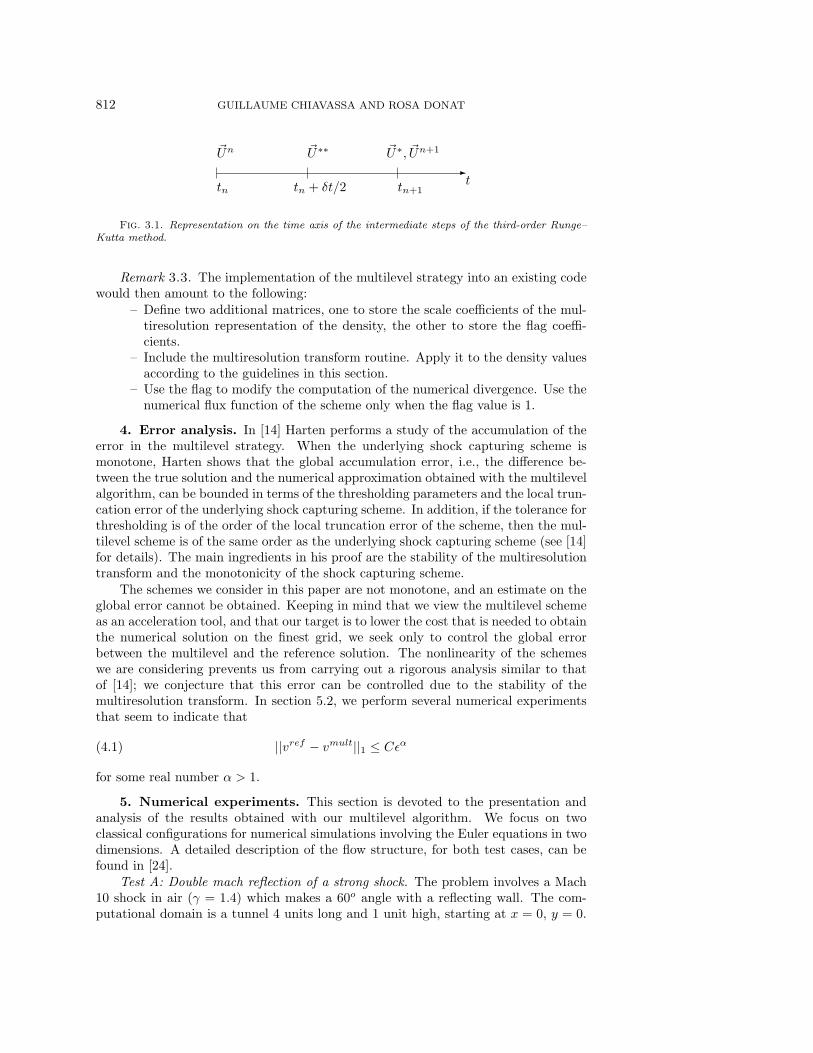
and the intermediate steps can be represented on the time axis as in Figure 3.1.Clearly, "U! is an order-1 approximation of "Un+1; thus it contains similar nonsmoothstructures at the same places, and the flag coe"cients obtained from its multiresolu-tion transform could be used to compute "Un+1 from "U!!, instead of deriving themfrom the "U!! multiresolution transform. This modification reduces the computationalcost of the multilevel algorithm while keeping the same quality in the numerical re-sults.


!"Un

tn

"U!!

tn + #t/2

"U!, "Un+1

tn+1t

Fig. 3.1. Representation on the time axis of the intermediate steps of the third-order Runge–Kutta method.

Remark 3.3. The implementation of the multilevel strategy into an existing codewould then amount to the following:

– Define two additional matrices, one to store the scale coe"cients of the mul-tiresolution representation of the density, the other to store the flag coe"-cients.

– Include the multiresolution transform routine. Apply it to the density valuesaccording to the guidelines in this section.

– Use the flag to modify the computation of the numerical divergence. Use thenumerical flux function of the scheme only when the flag value is 1.

4. Error analysis. In [14] Harten performs a study of the accumulation of theerror in the multilevel strategy. When the underlying shock capturing scheme ismonotone, Harten shows that the global accumulation error, i.e., the di!erence be-tween the true solution and the numerical approximation obtained with the multilevelalgorithm, can be bounded in terms of the thresholding parameters and the local trun-cation error of the underlying shock capturing scheme. In addition, if the tolerance forthresholding is of the order of the local truncation error of the scheme, then the mul-tilevel scheme is of the same order as the underlying shock capturing scheme (see [14]for details). The main ingredients in his proof are the stability of the multiresolutiontransform and the monotonicity of the shock capturing scheme.

The schemes we consider in this paper are not monotone, and an estimate on theglobal error cannot be obtained. Keeping in mind that we view the multilevel schemeas an acceleration tool, and that our target is to lower the cost that is needed to obtainthe numerical solution on the finest grid, we seek only to control the global errorbetween the multilevel and the reference solution. The nonlinearity of the schemeswe are considering prevents us from carrying out a rigorous analysis similar to thatof [14]; we conjecture that this error can be controlled due to the stability of themultiresolution transform. In section 5.2, we perform several numerical experimentsthat seem to indicate that

||vref ! vmult||1 ' C$!(4.1)

for some real number & > 1.

5. Numerical experiments. This section is devoted to the presentation andanalysis of the results obtained with our multilevel algorithm. We focus on twoclassical configurations for numerical simulations involving the Euler equations in twodimensions. A detailed description of the flow structure, for both test cases, can befound in [24].

Test A: Double mach reflection of a strong shock. The problem involves a Mach10 shock in air (' = 1.4) which makes a 60o angle with a reflecting wall. The com-putational domain is a tunnel 4 units long and 1 unit high, starting at x = 0, y = 0.


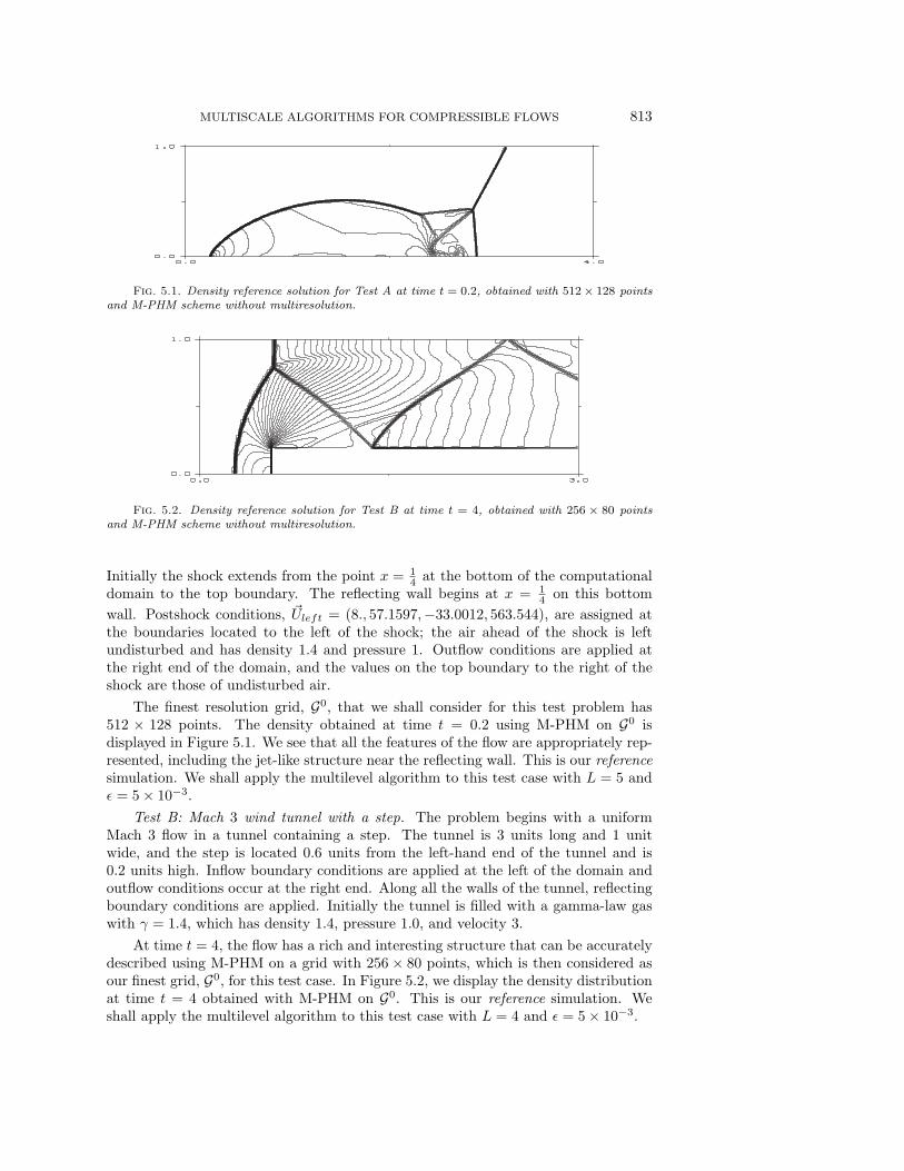
Fig. 5.1. Density reference solution for Test A at time t = 0.2, obtained with 512 ! 128 pointsand M-PHM scheme without multiresolution.

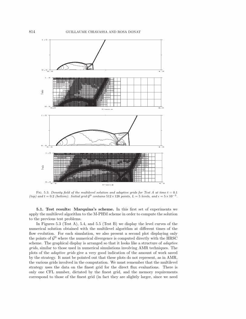
Fig. 5.2. Density reference solution for Test B at time t = 4, obtained with 256 ! 80 pointsand M-PHM scheme without multiresolution.

Initially the shock extends from the point x = 14 at the bottom of the computational

domain to the top boundary. The reflecting wall begins at x = 14 on this bottom

wall. Postshock conditions, "Uleft = (8., 57.1597,!33.0012, 563.544), are assigned atthe boundaries located to the left of the shock; the air ahead of the shock is leftundisturbed and has density 1.4 and pressure 1. Outflow conditions are applied atthe right end of the domain, and the values on the top boundary to the right of theshock are those of undisturbed air.

The finest resolution grid, G0, that we shall consider for this test problem has512 & 128 points. The density obtained at time t = 0.2 using M-PHM on G0 isdisplayed in Figure 5.1. We see that all the features of the flow are appropriately rep-resented, including the jet-like structure near the reflecting wall. This is our referencesimulation. We shall apply the multilevel algorithm to this test case with L = 5 and$ = 5 & 10#3.

Test B: Mach 3 wind tunnel with a step. The problem begins with a uniformMach 3 flow in a tunnel containing a step. The tunnel is 3 units long and 1 unitwide, and the step is located 0.6 units from the left-hand end of the tunnel and is0.2 units high. Inflow boundary conditions are applied at the left of the domain andoutflow conditions occur at the right end. Along all the walls of the tunnel, reflectingboundary conditions are applied. Initially the tunnel is filled with a gamma-law gaswith ' = 1.4, which has density 1.4, pressure 1.0, and velocity 3.

At time t = 4, the flow has a rich and interesting structure that can be accuratelydescribed using M-PHM on a grid with 256 & 80 points, which is then considered asour finest grid, G0, for this test case. In Figure 5.2, we display the density distributionat time t = 4 obtained with M-PHM on G0. This is our reference simulation. Weshall apply the multilevel algorithm to this test case with L = 4 and $ = 5 & 10#3.


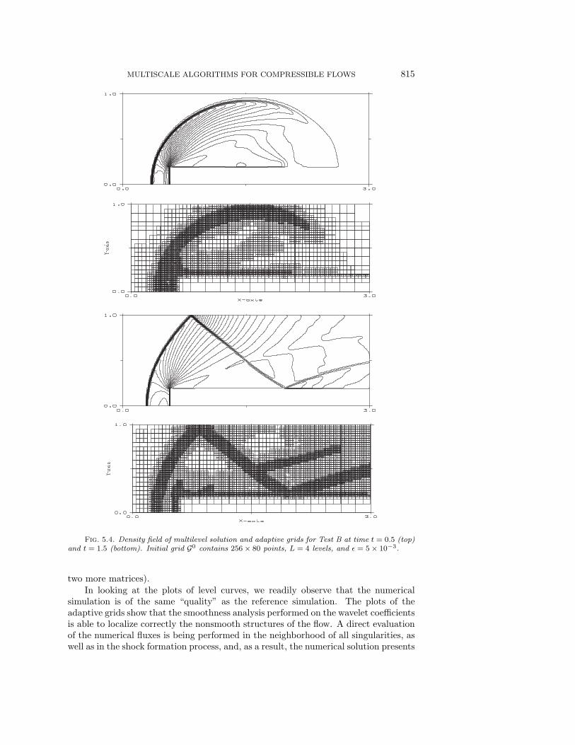
Fig. 5.3. Density field of the multilevel solution and adaptive grids for Test A at time t = 0.1(top) and t = 0.2 (bottom). Initial grid G0 contains 512!128 points, L = 5 levels, and " = 5!10"3.

5.1. Test results: Marquina’s scheme. In this first set of experiments weapply the multilevel algorithm to the M-PHM scheme in order to compute the solutionto the previous test problems.

In Figures 5.3 (Test A), 5.4, and 5.5 (Test B) we display the level curves of thenumerical solution obtained with the multilevel algorithm at di!erent times of theflow evolution. For each simulation, we also present a second plot displaying onlythe points of G0 where the numerical divergence is computed directly with the HRSCscheme. The graphical display is arranged so that it looks like a structure of adaptivegrids, similar to those used in numerical simulations involving AMR techniques. Theplots of the adaptive grids give a very good indication of the amount of work savedby the strategy. It must be pointed out that these plots do not represent, as in AMR,the various grids involved in the computation. We must remember that the multilevelstrategy uses the data on the finest grid for the direct flux evaluations. There isonly one CFL number, dictated by the finest grid, and the memory requirementscorrespond to those of the finest grid (in fact they are slightly larger, since we need


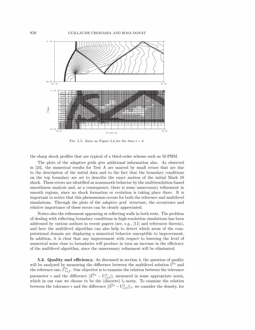
Fig. 5.4. Density field of multilevel solution and adaptive grids for Test B at time t = 0.5 (top)and t = 1.5 (bottom). Initial grid G0 contains 256 ! 80 points, L = 4 levels, and " = 5 ! 10"3.

two more matrices).In looking at the plots of level curves, we readily observe that the numerical

simulation is of the same “quality” as the reference simulation. The plots of theadaptive grids show that the smoothness analysis performed on the wavelet coe"cientsis able to localize correctly the nonsmooth structures of the flow. A direct evaluationof the numerical fluxes is being performed in the neighborhood of all singularities, aswell as in the shock formation process, and, as a result, the numerical solution presents


Fig. 5.5. Same as Figure 5.4 for the time t = 4.

the sharp shock profiles that are typical of a third-order scheme such as M-PHM.

The plots of the adaptive grids give additional information also. As observedin [24], the numerical results for Test A are marred by small errors that are dueto the description of the initial data and to the fact that the boundary conditionson the top boundary are set to describe the exact motion of the initial Mach 10shock. These errors are identified as nonsmooth behavior by the multiresolution-basedsmoothness analysis and, as a consequence, there is some unnecessary refinement insmooth regions, since no shock formation or evolution is taking place there. It isimportant to notice that this phenomenon occurs for both the reference and multilevelsimulations. Through the plots of the adaptive grid structure, the occurrence andrelative importance of these errors can be clearly appreciated.

Notice also the refinement appearing at reflecting walls in both tests. The problemof dealing with reflecting boundary conditions in high-resolution simulations has beenaddressed by various authors in recent papers (see, e.g., [11] and references therein),and here the multilevel algorithm can also help to detect which areas of the com-putational domain are displaying a numerical behavior susceptible to improvement.In addition, it is clear that any improvement with respect to lowering the level ofnumerical noise close to boundaries will produce in turn an increase in the e"ciencyof the multilevel algorithm, since the unnecessary refinement will be eliminated.

5.2. Quality and e!ciency. As discussed in section 4, the question of qualitywill be analyzed by measuring the di!erence between the multilevel solution "Un andthe reference one, "Un

ref . Our objective is to examine the relation between the tolerance

parameter $ and the di!erence ||"Un ! Unref ||, measured in some appropriate norm,

which in our case we choose to be the (discrete) l1-norm. To examine the relationbetween the tolerance $ and the di!erence ||"Un !Un

ref ||1, we consider the density, for


10-4 10-3 10-210-7

10-6

10-5

10-4

10-3

10-2

tolerance !

error

e 1

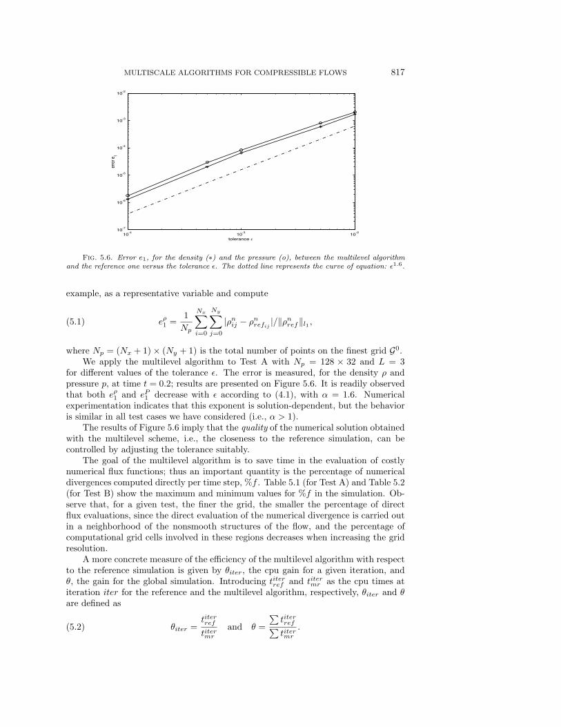
Fig. 5.6. Error e1, for the density (") and the pressure (o), between the multilevel algorithmand the reference one versus the tolerance ". The dotted line represents the curve of equation: "1.6.

example, as a representative variable and compute

e"1 =1

Np

Nx!

i=0

Ny!

j=0

|%nij ! %nrefij |/(%nref(l1 ,(5.1)

where Np = (Nx + 1) & (Ny + 1) is the total number of points on the finest grid G0.We apply the multilevel algorithm to Test A with Np = 128 & 32 and L = 3

for di!erent values of the tolerance $. The error is measured, for the density % andpressure p, at time t = 0.2; results are presented on Figure 5.6. It is readily observedthat both e"1 and eP1 decrease with $ according to (4.1), with & = 1.6. Numericalexperimentation indicates that this exponent is solution-dependent, but the behavioris similar in all test cases we have considered (i.e., & > 1).

The results of Figure 5.6 imply that the quality of the numerical solution obtainedwith the multilevel scheme, i.e., the closeness to the reference simulation, can becontrolled by adjusting the tolerance suitably.

The goal of the multilevel algorithm is to save time in the evaluation of costlynumerical flux functions; thus an important quantity is the percentage of numericaldivergences computed directly per time step, %f . Table 5.1 (for Test A) and Table 5.2(for Test B) show the maximum and minimum values for %f in the simulation. Ob-serve that, for a given test, the finer the grid, the smaller the percentage of directflux evaluations, since the direct evaluation of the numerical divergence is carried outin a neighborhood of the nonsmooth structures of the flow, and the percentage ofcomputational grid cells involved in these regions decreases when increasing the gridresolution.

A more concrete measure of the e"ciency of the multilevel algorithm with respectto the reference simulation is given by (iter, the cpu gain for a given iteration, and(, the gain for the global simulation. Introducing titerref and titermr as the cpu times atiteration iter for the reference and the multilevel algorithm, respectively, (iter and (are defined as

(iter =titerref

titermr

and ( =

"titerref"titermr

.(5.2)


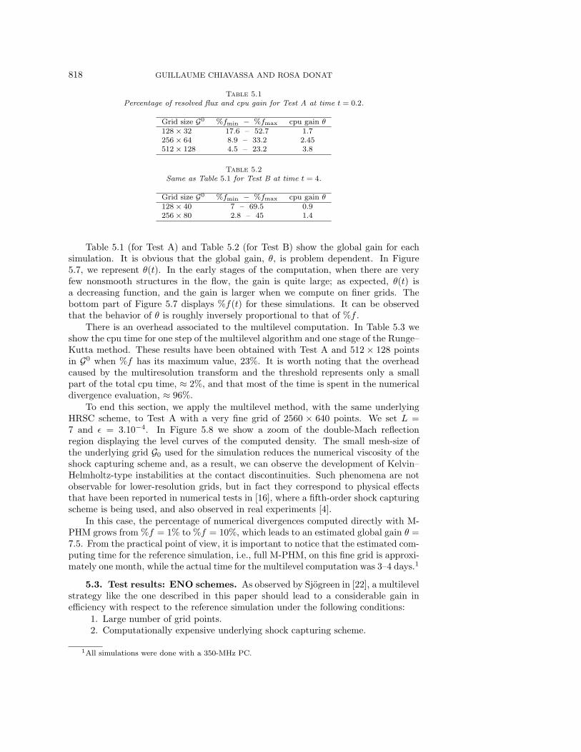
Table 5.1Percentage of resolved flux and cpu gain for Test A at time t = 0.2.

Grid size G0 %fmin # %fmax cpu gain #128 ! 32 17.6 – 52.7 1.7256 ! 64 8.9 – 33.2 2.45512 ! 128 4.5 – 23.2 3.8

Table 5.2Same as Table 5.1 for Test B at time t = 4.

Grid size G0 %fmin # %fmax cpu gain #128 ! 40 7 – 69.5 0.9256 ! 80 2.8 – 45 1.4

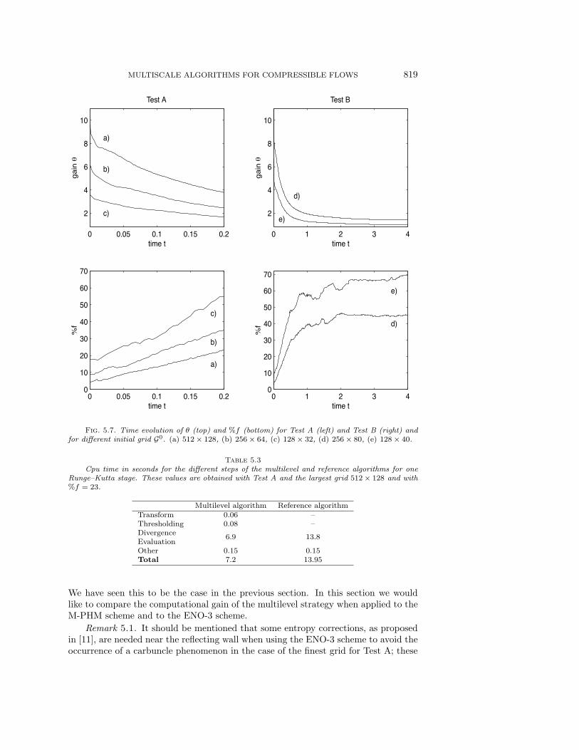
Table 5.1 (for Test A) and Table 5.2 (for Test B) show the global gain for eachsimulation. It is obvious that the global gain, (, is problem dependent. In Figure5.7, we represent ((t). In the early stages of the computation, when there are veryfew nonsmooth structures in the flow, the gain is quite large; as expected, ((t) isa decreasing function, and the gain is larger when we compute on finer grids. Thebottom part of Figure 5.7 displays %f(t) for these simulations. It can be observedthat the behavior of ( is roughly inversely proportional to that of %f .

There is an overhead associated to the multilevel computation. In Table 5.3 weshow the cpu time for one step of the multilevel algorithm and one stage of the Runge–Kutta method. These results have been obtained with Test A and 512 & 128 pointsin G0 when %f has its maximum value, 23%. It is worth noting that the overheadcaused by the multiresolution transform and the threshold represents only a smallpart of the total cpu time, ) 2%, and that most of the time is spent in the numericaldivergence evaluation, ) 96%.

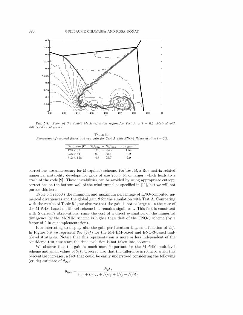
To end this section, we apply the multilevel method, with the same underlyingHRSC scheme, to Test A with a very fine grid of 2560 & 640 points. We set L =7 and $ = 3.10#4. In Figure 5.8 we show a zoom of the double-Mach reflectionregion displaying the level curves of the computed density. The small mesh-size ofthe underlying grid G0 used for the simulation reduces the numerical viscosity of theshock capturing scheme and, as a result, we can observe the development of Kelvin–Helmholtz-type instabilities at the contact discontinuities. Such phenomena are notobservable for lower-resolution grids, but in fact they correspond to physical e!ectsthat have been reported in numerical tests in [16], where a fifth-order shock capturingscheme is being used, and also observed in real experiments [4].

In this case, the percentage of numerical divergences computed directly with M-PHM grows from %f = 1% to %f = 10%, which leads to an estimated global gain ( =7.5. From the practical point of view, it is important to notice that the estimated com-puting time for the reference simulation, i.e., full M-PHM, on this fine grid is approxi-mately one month, while the actual time for the multilevel computation was 3–4 days.1

5.3. Test results: ENO schemes. As observed by Sjogreen in [22], a multilevelstrategy like the one described in this paper should lead to a considerable gain ine"ciency with respect to the reference simulation under the following conditions:

1. Large number of grid points.2. Computationally expensive underlying shock capturing scheme.

1All simulations were done with a 350-MHz PC.


0 0.05 0.1 0.15 0.2

2

4

6

8

10

time t

gain

"

Test A

a)

b)

c)

0 1 2 3 4

2

4

6

8

10

time t ga

in "

Test B

e)

d)

0 0.05 0.1 0.15 0.2 0

10

20

30

40

50

60

70

time t

%f

a)

b)

c)

0 1 2 3 4 0

10

20

30

40

50

60

70

time t

%f d)

e)

Fig. 5.7. Time evolution of # (top) and %f (bottom) for Test A (left) and Test B (right) andfor di!erent initial grid G0. (a) 512 ! 128, (b) 256 ! 64, (c) 128 ! 32, (d) 256 ! 80, (e) 128 ! 40.

Table 5.3Cpu time in seconds for the di!erent steps of the multilevel and reference algorithms for one

Runge–Kutta stage. These values are obtained with Test A and the largest grid 512 ! 128 and with%f = 23.

Multilevel algorithm Reference algorithmTransform 0.06 –Thresholding 0.08 –DivergenceEvaluation

6.9 13.8

Other 0.15 0.15Total 7.2 13.95

We have seen this to be the case in the previous section. In this section we wouldlike to compare the computational gain of the multilevel strategy when applied to theM-PHM scheme and to the ENO-3 scheme.

Remark 5.1. It should be mentioned that some entropy corrections, as proposedin [11], are needed near the reflecting wall when using the ENO-3 scheme to avoid theoccurrence of a carbuncle phenomenon in the case of the finest grid for Test A; these


2.2 2.3 2.4 2.5 2.6 2.7 2.8 2.9 3 0

0.05

0.1

0.15

0.2

0.25

0.3

0.35

0.4

0.45

0.5

x

y

Fig. 5.8. Zoom of the double Mach reflection region for Test A at t = 0.2 obtained with2560 ! 640 grid points.

Table 5.4Percentage of resolved fluxes and cpu gain for Test A with ENO-3 fluxes at time t = 0.2.

Grid size G0 %fmin # %fmax cpu gain #128 ! 32 17.6 – 54.2 1.54256 ! 64 8.9 – 38.4 2.2512 ! 128 4.5 – 25.7 2.9

corrections are unnecessary for Marquina’s scheme. For Test B, a Roe-matrix-relatednumerical instability develops for grids of size 256 & 64 or larger, which leads to acrash of the code [9]. These instabilities can be avoided by using appropriate entropycorrections on the bottom wall of the wind tunnel as specified in [11], but we will notpursue this here.

Table 5.4 reports the minimum and maximum percentage of ENO-computed nu-merical divergences and the global gain ( for the simulation with Test A. Comparingwith the results of Table 5.1, we observe that the gain is not as large as in the case ofthe M-PHM-based multilevel scheme but remains significant. This fact is consistentwith Sjogreen’s observations, since the cost of a direct evaluation of the numericaldivergence by the M-PHM scheme is higher than that of the ENO-3 scheme (by afactor of 2 in our implementation).

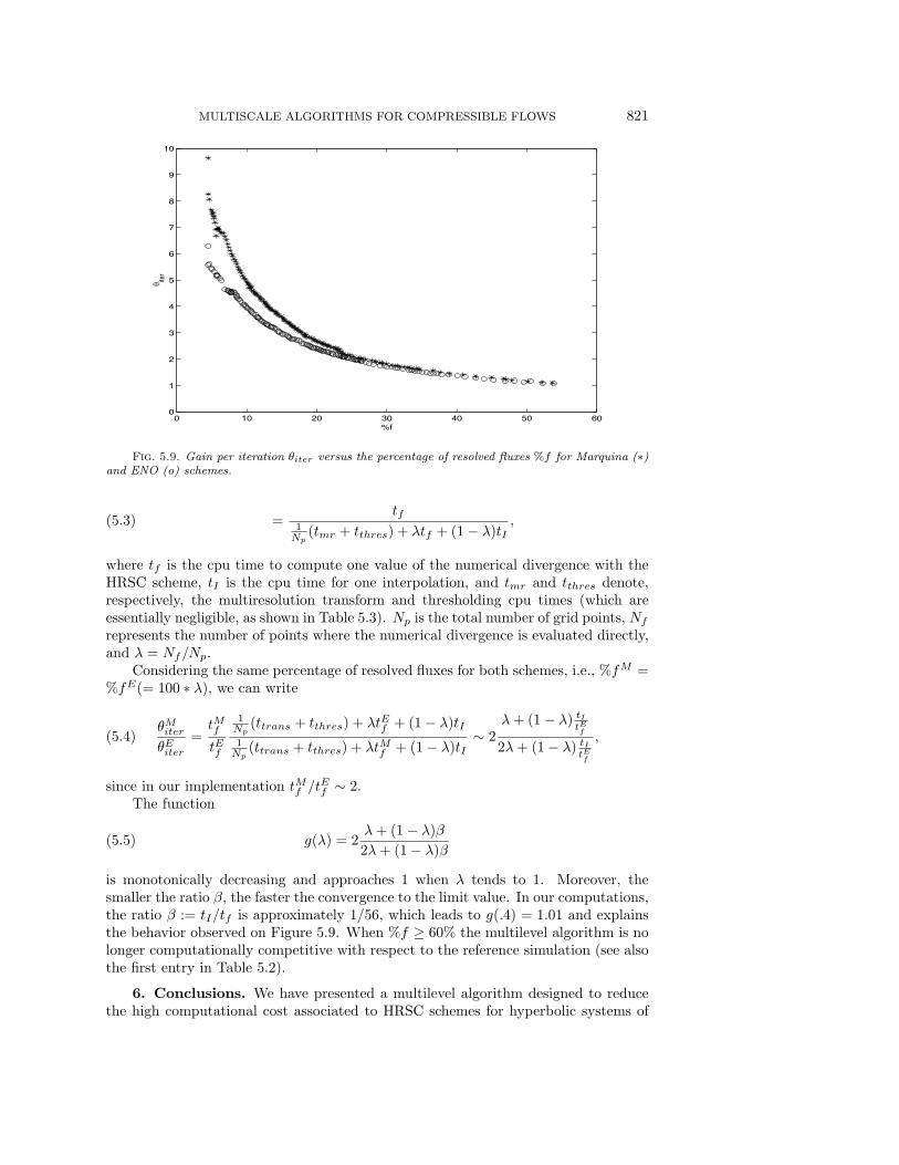
It is interesting to display also the gain per iteration (iter as a function of %f .In Figure 5.9 we represent (iter(%f) for the M-PHM-based and ENO-3-based mul-tilevel strategies. Notice that this representation is more or less independent of theconsidered test case since the time evolution is not taken into account.

We observe that the gain is much more important for the M-PHM multilevelscheme and small values of %f . Observe also that the di!erence is reduced when thispercentage increases, a fact that could be easily understood considering the following(crude) estimate of (iter:

(iter =Nptf

tmr + tthres + Nf tf + (Np !Nf )tI


0 10 20 30 40 50 60 0

1

2

3

4

5

6

7

8

9

10

%f

" iter

Fig. 5.9. Gain per iteration #iter versus the percentage of resolved fluxes %f for Marquina (")and ENO (o) schemes.

=tf

1Np

(tmr + tthres) + )tf + (1 ! ))tI,(5.3)

where tf is the cpu time to compute one value of the numerical divergence with theHRSC scheme, tI is the cpu time for one interpolation, and tmr and tthres denote,respectively, the multiresolution transform and thresholding cpu times (which areessentially negligible, as shown in Table 5.3). Np is the total number of grid points, Nf

represents the number of points where the numerical divergence is evaluated directly,and ) = Nf/Np.

Considering the same percentage of resolved fluxes for both schemes, i.e., %fM =%fE(= 100 * )), we can write

(Miter(Eiter

=tMftEf

1Np

(ttrans + tthres) + )tEf + (1 ! ))tI1Np

(ttrans + tthres) + )tMf + (1 ! ))tI+ 2

)+ (1 ! )) tItEf

2)+ (1 ! )) tItEf

,(5.4)

since in our implementation tMf /tEf + 2.The function

g()) = 2)+ (1 ! ))*2)+ (1 ! ))*(5.5)

is monotonically decreasing and approaches 1 when ) tends to 1. Moreover, thesmaller the ratio *, the faster the convergence to the limit value. In our computations,the ratio * := tI/tf is approximately 1/56, which leads to g(.4) = 1.01 and explainsthe behavior observed on Figure 5.9. When %f % 60% the multilevel algorithm is nolonger computationally competitive with respect to the reference simulation (see alsothe first entry in Table 5.2).

6. Conclusions. We have presented a multilevel algorithm designed to reducethe high computational cost associated to HRSC schemes for hyperbolic systems of


conservation laws, and we have investigated the application of this multilevel strategyto state-of-the-art HRSC schemes using standard tests for the 2D Euler equations.

The numerical results presented in this paper point out that there is a significantreduction of the computational time when using the multilevel algorithm and confirmSjogreen’s observations in [22]: the more expensive the flux computation, the betterthe e"ciency of the multilevel computation with respect to the reference simulation.

Our multilevel strategy follows the basic design principle of Bihari and Hartenin [5], but it is built upon the interpolatory multiresolution framework, instead ofthe cell-average framework, as in [1, 2, 5, 6, 22, 17]. Through a series of numericalexperiments, we show that the strategy we propose o!ers the possibility of obtain-ing a high-resolution numerical solution on a very fine grid at the cost of the user’sown numerical technique on a much coarser mesh. Its potential users might be re-searchers performing computational tests with state-of-the-art HRSC methods andusing uniform grids.

As in [1, 2, 5, 22], our technique works on the discrete values at the highestresolution level, which need to be always available. There are no memory savingswith respect to the reference simulation. In [6, 17], the authors concentrate on solvingthe evolution equations associated to the (cell-average) scale coe"cients. While thisoption opens the door to what might be an alternative to AMR, a fully adaptivealgorithm with selective refinement and real memory savings, it also su!ers, in ouropinion, from some of the drawbacks of AMR: the need of a special data structurewhich invariably leads to a very complicated coding structure.

On the other hand, our approach (due in part to the use of the interpolatoryframework) is pretty transparent, even to the nonexpert in multiscale analysis, andits incorporation into an existing hydrodynamical code is, in principle, much easier.

REFERENCES

[1] R. Abgrall, Multiresolution in unstructured meshes: Application to CFD, in Numerical Meth-ods for Fluid Dynamics, Vol. 5, K. W. Morton and M. J. Baines, eds., Oxford Sci. Publ.,Oxford University Press, New York, 1995, pp. 271–276.

[2] R. Abgrall, S. Lanteri, and T. Sonar, ENO schemes for compressible fluid dynamics, Z.Angew. Math. Mech., 79 (1999), pp. 3–28.

[3] F. Arandiga, R. Donat, and A. Harten, Multiresolution based on weighted averages ofthe hat function I: Linear reconstruction techniques, SIAM J. Numer. Anal., 36 (1998),pp. 160–203.

[4] G. Ben-Dor, Shock Wave Reflection Phenomena, Springer-Verlag, New York, 1992.[5] B. Bihari and A. Harten, Multiresolution schemes for the numerical solutions of 2D conser-

vation laws, SIAM J. Sci. Comput., 18 (1997), pp. 315–354.[6] W. Dahmen, B. Gottschlich-Muller, and S. Muller, Multiresolution Schemes for Con-

servation Laws, Technical report, Bericht 159 IGMP, RWTH Aachen, Germany, 1998.[7] A. Dolezal and S. Wong, Relativistic hydrodynamics and essentially non-oscillatory shock

capturing schemes, J. Comput. Phys., 120 (1995), pp. 266–277.[8] R. Donat and A. Marquina, Capturing shock reflections: An improved flux formula, J. Com-

put. Phys., 125 (1996), pp. 42–58.[9] R. Donat and A. Marquina, Computing Strong Shocks in Ultrarelativistic Flows: A Robust

Alternative, Internat. Ser. Numer. Math. 129, Birkhauser, Basel, 1999.[10] F. Eulderink, Numerical Relativistic Hydrodynamics, Ph.D. thesis, University of Leiden, Lei-

den, The Netherlands, 1993.[11] R. Fedkiw, A. Marquina, and B. Merriman, An isobaric fix for the overheating problem in

multimaterial compressible flows, J. Comput. Phys., 148 (1999), pp. 545–578.[12] R. Fedkiw, B. Merriman, R. Donat, and S. Osher, The Penultimate Scheme for Systems of

Conservation Laws: Finite Di!erence ENO with Marquina’s Flux Splitting, UCLA CAMReport 96-18, UCLA, Los Angeles, CA, 1996.


[13] A. Harten, Discrete multiresolution analysis and generalized wavelets, J. Appl. Numer. Math.,12 (1993), pp. 153–192.

[14] A. Harten, Multiresolution algorithms for the numerical solution of hyperbolic conservationlaws, Comm. Pure Appl. Math., 48 (1995), pp. 1305–1342.

[15] A. Harten, Multiresolution representation of data: A general framework, SIAM J. Numer.Anal., 33 (1996), pp. 1205–1256.

[16] C. Hu and C.-W. Shu, Weighted essentially non-oscillatory schemes on triangular meshes, J.Comput. Phys., 150 (1999), pp. 97–127.

[17] S. Kaber and M. Postel, Finite volume schemes on triangles coupled with multiresolutionanalysis, C. R. Acad. Sci. Paris Ser. I Math., 328 (1999), pp. 817–822.

[18] A. Marquina, Local piecewise hyperbolic reconstruction of numerical fluxes for nonlinear scalarconservation laws, SIAM J. Sci. Comput., 15 (1994), pp. 892–915.

[19] J. Marti, E. Muller, J. Font, J. Ibanez, and A. Marquina, Morphology and dynamics ofrelativistic jets, Astrophys. J., 479 (1997), pp. 151–163.

[20] J. Quirk, A contribution of the great Riemann solver debate, Internat. J. Numer. MethodsFluids, 18 (1994), pp. 555–574.

[21] C.-W. Shu and S. J. Osher, E"cient implementation of essentially nonoscillatory shock-capturing schemes. II, J. Comput. Phys., 83 (1989), pp. 32–78.

[22] B. Sjogreen, Numerical experiments with the multiresolution scheme for the compressibleeuler equations, J. Comput. Phys., 117 (1995), pp. 251–261.

[23] W. Sweldens, The lifting scheme: A construction of second generation wavelets, SIAM J.Math. Anal., 29 (1998), pp. 511–546.

[24] P. R. Woodward and P. Colella, The numerical simulation of two-dimensional fluid flowwith strong shocks, J. Comput. Phys., 54 (1984), pp. 115–173.

point value multiscale algorithms for 2d compressible flowsgchiavassa/sisc.pdf · point value...

Documents