pnnl report on the development of bench-scale cfd ... ... bound for overall mass transfer...
TRANSCRIPT
PNNL Report on the Development of Bench-scale CFD Simulations for Gas Absorption across a Wetted Wall Column
Work Performed Under
Activity Number 0004000.6.600.007.002 ARRA
Prepared by Pacific Northwest National Laboratory
Richland, Washington 99352
In collaboration with Los Alamos National Laboratory, Lawrence Livermore National Laboratory, the National Energy Technology Laboratory, and Princeton University
Prepared for the
U.S. Department of Energy National Energy Technology Laboratory
January 2016

PNNL Milestone Report
1
Revision Log
Revision Date Revised By: Description
0.1 Jan 2016 Chao Wang Original draft
0.2 Jan 20 2016 Zhijie Xu Revised
0.3
0.4
1.0
Disclaimer
This report was prepared as an account of work sponsored by an agency of the United States Government. Neither the United States Government nor any agency thereof, nor any of their employees, makes any warranty, express or implied, or assumes any legal liability or responsibility for the accuracy, completeness, or usefulness of any information, apparatus, product, or process disclosed, or represents that its use would not infringe privately owned rights. Reference herein to any specific commercial product, process, or service by trade name, trademark, manufacturer, or otherwise does not necessarily constitute or imply its endorsement, recommendation, or favoring by the United States Government or any agency thereof. The views and opinions of authors expressed herein do not necessarily state or reflect those of the United States Government or any agency thereof.
Acknowledgment of Funding This project was funded under the Carbon Capture Simulation Initiative under the following FWPs and contracts:
LANL - FE-101-002-FY10 PNNL - 60115 LLNL - FEW0180 LBNL - CSNW1130 NETL - RES-0004000.6.600.007.002
PNNL Milestone Report
2
Table of Contents
1. INTRODUCTION ........................................................................................................................... 5
2. EXPERIMENTAL STUDY OF WWC .......................................................................................... 6
2.1 Design of Experiments .............................................................................................................................. 6
2.2 Experimental Results ................................................................................................................................ 8 2.2.1 N2O/MEA system ......................................................................................................................................8 2.2.2 CO2/MEA system .......................................................................................................................................9
3. NUMERICAL MODELING OF WWC ....................................................................................... 11
3.1 General Theory on Mass Transport and Chemistry ................................................................................. 11
3.2 Calculation of Model Input Parameters ................................................................................................... 14 3.2.1 MEA Solvent Density ...............................................................................................................................14 3.2.2 MEA Solvent Kinematic Viscosity ............................................................................................................14 3.2.3 Gas Diffusivity in Solvent ........................................................................................................................14 3.2.4 Gas Henry’s Constant in Solvent .............................................................................................................15 3.2.5 MEA Diffusivity in Solvent .......................................................................................................................15 3.2.6 Gas Density .............................................................................................................................................15 3.2.7 Gas Dynamics Viscosity ...........................................................................................................................15 3.2.8 Gas Diffusivity .........................................................................................................................................16 3.2.9 Surface Tension .......................................................................................................................................16
3.3 CFD Model Setup .................................................................................................................................... 17 3.3.1 Geometry ................................................................................................................................................17 3.3.2 Boundary and Initial Conditions ..............................................................................................................18 3.3.3 Input Parameters of the CFD model .......................................................................................................18 3.3.4 Computational Methods .........................................................................................................................20
3.4 Calculation of Overall Mass Transfer Coefficient ..................................................................................... 20 3.4.1 N2O/MEA System ....................................................................................................................................20 3.4.2 CO2/MEA System.....................................................................................................................................22
3.5 Results Analysis ...................................................................................................................................... 22 3.5.1 O2/H2O System .......................................................................................................................................23
3.5.1.1 Effect of Injection Frequency on Surface Waves ............................................................................24 3.5.1.2 Variation of O2 Concentration for Different Frequencies ...............................................................25 3.5.1.3 Variation of O2 Concentration with Controlled Amplitude .............................................................25
3.5.2 N2O/MEA System ....................................................................................................................................26 3.5.3 CO2/MEA System.....................................................................................................................................30
3.6 Parametric Analysis................................................................................................................................. 32 3.6.1 N2O/MEA System ....................................................................................................................................32 3.6.2 CO2/MEA System.....................................................................................................................................33
3.7 Summary of the Results .......................................................................................................................... 34
PNNL Milestone Report
3
4. MODEL CALIBRATION AND UQ ANALYSIS FOR WWC EXPERIMENTS .................... 35
4.1 N2O/MEA System .................................................................................................................................... 35
4.2 CO2/MEA System .................................................................................................................................... 39
ACKNOWLEDGMENTS ................................................................................................................. 42
REFERENCES ................................................................................................................................... 42
APPENDIX........................................................................................................................................ 43
List of Figures
Figure 1 Schematic of CFD simulation hierarchy ................................................................................................ 5 Figure 2 Schematic of the WWC.................................................................................................................................. 7 Figure 3 Schematic of WWC Test Setup ................................................................................................................... 7 Figure 4 P* versus CO2 Loading ............................................................................................................................... 10 Figure 5 Countercurrent Gas Flow Geometry Schematics ............................................................................ 18 Figure 6 Mesh Size Distribution in x Direction .................................................................................................. 20 Figure 7 Sharp Gas-Liquid Interface versus Gas-Liquid Interface Layer ................................................ 21 Figure 8 Profiles of Falling Film with Increasing Frequencies in Injection Rates (more surface waves can be observed at higher frequencies).................................................................................................. 24 Figure 9 Variation of Gas Concentration Distribution for Different Fluctuation Frequencies (a larger frequency leads to a steeper concentration gradient in the vertical direction and a larger mass transfer across the interface) ........................................................................................................................ 25 Figure 10 Variation of Gas Concentration Distribution for Different Fluctuation Amplitudes in the Injection Rate (a larger amplitude leads to a steeper concentration gradient along the vertical direction) .......................................................................................................................................................... 26 Figure 11 Numerical Simulation Versus Experimental Data for Overall Mass Transfer Coefficient in N2O/MEA System ...................................................................................................................................................... 27 Figure 12 kG versus Controlled Parameters in N2O/MEA Systems ............................................................ 29 Figure 13 kG versus Henry’s Constant and Diffusivity .................................................................................... 29 Figure 14 Numerical Simulation Versus Experimental Data for Overall Mass Transfer Coefficient in CO2/MEA Systems .................................................................................................................................................... 30 Figure 15 kG versus Controlled Parameters in CO2/MEA Systems ............................................................ 32 Figure 16 N2O/MEA Parametric Study ................................................................................................................. 33 Figure 17 CO2/MEA Parametric Study .................................................................................................................. 34 Figure 18 Estimated Marginal Posterior Distributions for the Calibration Parameters of the Non-reacting Scenario (blue line segments are the point estimates found in the literature) ....... 38

PNNL Milestone Report
4
Figure 19 Predictive Diagnostic Plots for the Non-reaction Scenario (both panels compare the experimental data points (black “x”) to predicted simulator output (red); refer to the text for more in-depth descriptions) ..................................................................................................................................... 38 Figure 20 Estimated Marginal Posterior Distributions for the Calibration Parameters of the Reacting Scenario (blue line segments are the point estimates found in the literature) ................. 40 Figure 21 Uncertainty, the Rate Constant, as a Function of Temperature (C) (blue curve is derived from the literature, while the black curve is the median prediction; the dashed lines form pointwise 90% intervals) ................................................................................................................................ 41 Figure 22 Predictive Diagnostic Plots for the Reacting Scenario (both panels compare the experimental data points (black “x”) to predicted simulator output (red); refer to the text for more in-depth descriptions) ..................................................................................................................................... 41
List of Tables Table 1 Key WWC Dimensions .................................................................................................................................... 6 Table 2 N2O/MEA Experimental Data ...................................................................................................................... 9 Table 3 CO2/MEA Experimental Data .................................................................................................................... 11 Table 4 Regressed Parameter for Equilibrium Constant 𝑲𝑲𝑲𝑲𝑲𝑲𝟐𝟐 ................................................................. 13 Table 5 Parameters for Solvent Density Correlation ....................................................................................... 14 Table 6 𝛔𝛔𝛔𝛔 and 𝛏𝛏𝛔𝛔/𝐤𝐤𝐤𝐤 Values ...................................................................................................................................... 16 Table 7 Controlled Input Parameters .................................................................................................................... 19 Table 8 Direct Model Input Parameters................................................................................................................ 19 Table 9 Values of Input Parameters........................................................................................................................ 23 Table 10 Inputs to the Computer Model for the Non-reacting Case ........................................................ 36 Table 11 Default Relationships between Calibration Inputs and Experimental Inputs for the Non-reacting Scenario ................................................................................................................................................. 37 Table 12 Priors for Calibration Parameters ....................................................................................................... 37 Table 13 Inputs to the Computer Model for the Reacting Case ................................................................. 39 Table 14 Default Relationships for the Reacting Scenario ........................................................................... 39

PNNL Milestone Report
5
PNNL Report on the Development of Bench-scale CFD Simulations for Gas Absorption across a Wetted Wall Column Chao Wanga, Zhijie Xua, Kevin Laia, Greg Whyatta, Peter William Marcyb, James Gattikerb, Xin Suna
aPacific Northwest National Laboratory, Richland, WA bLos Alamos National Laboratory, Los Alamos, NM
1. Introduction The Carbon Capture Simulation Initiative (CCSI) develops state-of-the-art computational modeling and simulation tools to accelerate commercialization of carbon capture technologies from discovery to development with eventual widespread deployment to hundreds of power plants through a partnership among national laboratories, industry, and academic institutions. The ultimate goal of the CCSI toolset is to provide end users in industry with a comprehensive, integrated suite of scientifically validated models and deliver uncertainty quantification (UQ), optimization, risk analysis, and decision-making capabilities. In order to enable the hierarchical prediction of carbon capture efficiency of a solvent-based absorption column, a computational fluid dynamics (CFD) model is first developed to simulate the core phenomena of solvent-based carbon capture, i.e., the CO2 physical absorption and chemical reaction, on a simplified geometry of wetted wall column (WWC) at bench scale. Aqueous solutions of ethanolamine (MEA) are commonly selected as a CO2 stream scrubbing liquid. CO2 is captured by both physical and chemical absorption using highly CO2 soluble and reactive solvent, MEA, during the scrubbing process. In order to provide confidence bound on the computational predictions of this complex engineering system, a hierarchical calibration and validation framework is proposed in [1]. The overall goal of this effort is to provide a mechanism-based predictive framework with confidence bound for overall mass transfer coefficient of the wetted wall column (WWC) with statistical analyses of the corresponding WWC experiments with increasing physical complexity. A series of unit problems is proposed to break the complex multi-physics in solvent-based CO2 capture into simpler single physical problems as shown in Figure 1 [1]. The final outcome of this work is the distributions of the effective mass transfer coefficient for a given solvent (MEA here) and the associated posterior distributions of solvent properties including Henry’s constant, diffusivity and reaction rate constants.
Figure 1 Schematic of CFD simulation hierarchy
Unit problem 1, i.e., flow hydrodynamics of a falling film, has been extensively investigated in the literature. In this study, volume of fluids (VOF)-based CFD simulations were performed for film flowing down the column with various viscosities. The model results are validated by comparison between the simulated steady state film thickness and the theoretical prediction for various viscosities. After that, quantitative confidence in the
Unit problem 1 --WWC
hydrodynamics
Unit problem 2 -- non-reactive flow
and mass transfer
Unit problem 3 -- coupled reaction, mass transfer, flow
PNNL Milestone Report
6
numerical accuracy and code implementation of the open source package (OpenFOAM) for simulating flow hydrodynamics were established. In the present report, we focus on presenting the detailed analysis results of Unit problems 2 and 3. The focus of Unit problem 2 is the coupling of two physical processes, i.e., mass transfer and hydrodynamics between gas and liquid. The gas-liquid pairs of interest include O2/Water and N2O/MEA. In this unit problem, we will first investigate the effects of surface wave frequency and amplitude on the overall mass transfer between O2 and water in WWC with various water injection rates. The coupled mass transfer with hydrodynamics model will be further validated and calibrated with controlled WWC experiments with N2O/MEA system. Here N2O is used as a surrogate for CO2 without the absorption reaction. Upon completion of Unit problem 2, posterior distributions of Henry’s constant and diffusivity can be established with the coupled hydrodynamics and mass transfer model and the corresponding experiments. Next, Unit problem 3 will be carried out with the same WWC set up, but with the introduction of CO2 in the gas stream. The transport properties of CO2 in MEA system can be inferred from the posterior distributions obtained in Unit problem 2 for N2O based on available literatures [2, 3]. In doing so, the effects of CO2 mass transfer and chemical absorption within MEA can be separated. After this step, more physical insights can be obtained and a systematic calibration of reaction rate constants will be implemented for the CO2/MEA system. Upon completion of the entire hierarchical simulations of the WWC system, the multiphase CFD models with coupled chemistry and mass transport capabilities can be established to predict the overall CO2 mass transfer rate of the WWC.
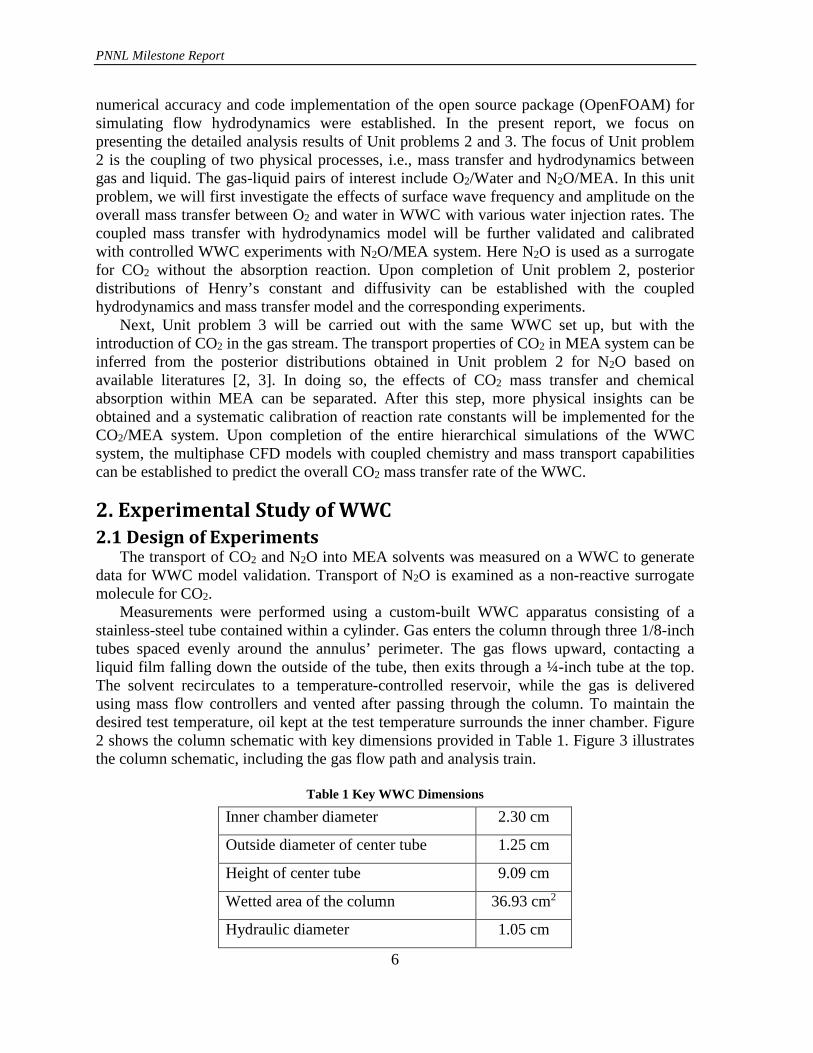
2. Experimental Study of WWC 2.1 Design of Experiments
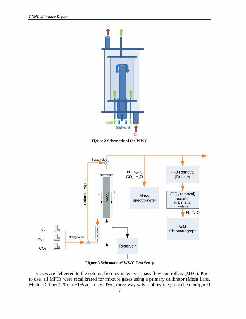
The transport of CO2 and N2O into MEA solvents was measured on a WWC to generate data for WWC model validation. Transport of N2O is examined as a non-reactive surrogate molecule for CO2. Measurements were performed using a custom-built WWC apparatus consisting of a stainless-steel tube contained within a cylinder. Gas enters the column through three 1/8-inch tubes spaced evenly around the annulus’ perimeter. The gas flows upward, contacting a liquid film falling down the outside of the tube, then exits through a ¼-inch tube at the top. The solvent recirculates to a temperature-controlled reservoir, while the gas is delivered using mass flow controllers and vented after passing through the column. To maintain the desired test temperature, oil kept at the test temperature surrounds the inner chamber. Figure 2 shows the column schematic with key dimensions provided in Table 1. Figure 3 illustrates the column schematic, including the gas flow path and analysis train.
Table 1 Key WWC Dimensions
Inner chamber diameter 2.30 cm
Outside diameter of center tube 1.25 cm
Height of center tube 9.09 cm
Wetted area of the column 36.93 cm2
Hydraulic diameter 1.05 cm
PNNL Milestone Report
7
Figure 2 Schematic of the WWC
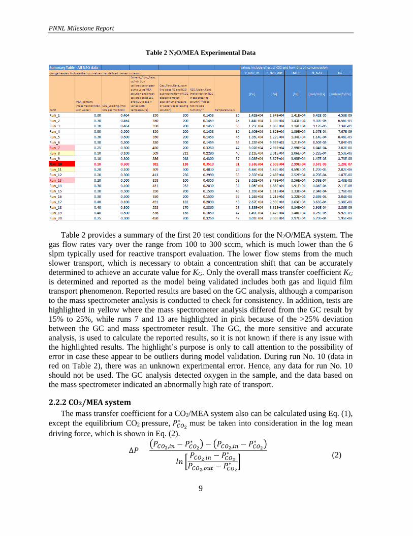
Figure 3 Schematic of WWC Test Setup
Gases are delivered to the column from cylinders via mass flow controllers (MFC). Prior to use, all MFCs were recalibrated for mixture gases using a primary calibrator (Mesa Labs, Model Definer 220) to ±1% accuracy. Two, three-way valves allow the gas to be configured
Reservoir
Mass Spectrometer
Gas Chromatograph
H2O Removal(Drierite)
(CO2 removal)ascarite
Only for N2O analysis
N2, N2O
Col
umn
Byp
ass
WW
C
N2, N2O,CO2, H2O
N2
N2O
CO2
3 way valve
3 way valve
Hum
idifi
er

PNNL Milestone Report
8
to flow either through the column or a bypass leg. During a test, the gas is first flowed through the bypass leg, then switched to the column, and then back to the bypass leg. The shift in concentration while the gas is routed through the column then is used to deduce the rate at which the gas is being absorbed by the column. Liquid flow to the column is set via a speed control on a gear pump (Cole Parmer model 75211-30 with #074012-51 pump head). The gear pump flow is calibrated versus pump speed prior to the test. Then, the speed corresponding to the desired flow is set. After tests 1 through 6 had been performed without humidifying the gas that entered the column, a Nafion humidifier (model FC125-240-5MP) was added to the system to bring the water vapor pressure of the gas entering the column to a level near that of the equilibrium vapor pressure of the solution being tested. A heated water bath circulated water through the shell side of the humidifier, while the process gas passed through the Nafion tubes. The addition of the humidifier was intended to reduce uncertainty in the concentration driving force related to the timing of the dry gas’ dilution with water vapor and to avoid a reduction in mass transfer that could occur due to phase drift as water is transported away from the liquid film in the gas phase. For the purposes of data analysis, the concentration driving force for the first six tests assumed that the gas was humidified immediately upon entering the column. Gas composition of the stream exiting the WWC has been analyzed using a quadrupole mass spectrometer (MKS, Cirrus 200 amu) sampling at atmospheric pressure. The mass spectrometer provides an analysis of gas composition at four-second intervals. Because CO2 and N2O both have an atomic mass of 44, N2O is analyzed on the mass spectrometer at mass 30, corresponding to a nitric oxide (NO) splitting peak. The mass spectrometer samples the gas directly without drying. A gas chromatograph (Agilent Model 3000A Micro GC) also is used to provide analysis of the gas composition, providing data at four-minute intervals. Of the two instruments, the GC offers a more accurate and sensitive measurement, but the mass spectrometer provides better transient information due to the faster sampling rate. Prior to GC analysis, the sampled gas is dried using a Drierite column. When measuring N2O transport, the gas also passes through an Ascarite bed to remove CO2 and prevent possible overlap of N2O and CO2 peaks on the GC. The amount of N2O absorbed is deduced by the shift in the ratio of N2O to N2 as measured on the GC. Reagent grade (98%) MEA was purchased from Spectrum Chemical Manufacturing Corp. and blended with deionized water to provide the desired solvent concentration. N2O (99.6%), CO2, and N2 gases (99.998%) were purchased from OXARC and used without further purification. The initial solvent loading was achieved via mass addition of dry ice to the solvent. The dry ice (99% purity) also was purchased from OXARC. 2.2 Experimental Results
2.2.1 N2O/MEA system The mass transfer coefficient 𝐾𝐾𝐺𝐺 (mol/Pa·s·m2) is calculated by 𝐾𝐾𝐺𝐺 = 𝐽𝐽
∆𝑃𝑃, (1)
where ∆𝑃𝑃 = �𝑃𝑃𝑁𝑁2𝑂𝑂,𝑖𝑖𝑖𝑖 − 𝑃𝑃𝑁𝑁2𝑂𝑂,𝑜𝑜𝑜𝑜𝑜𝑜�/ln�𝑃𝑃𝑁𝑁2𝑂𝑂,𝑖𝑖𝑖𝑖/𝑃𝑃𝑁𝑁2𝑂𝑂,𝑜𝑜𝑜𝑜𝑜𝑜� denotes log mean driving force and 𝐽𝐽 (mol/m2·s) denotes the mass transfer flux at the gas-liquid interface.
PNNL Milestone Report
9
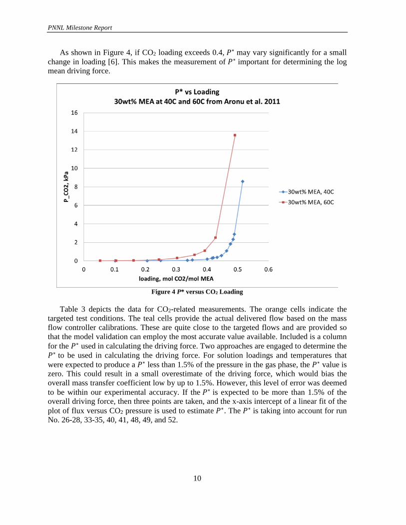
Table 2 N2O/MEA Experimental Data
Table 2 provides a summary of the first 20 test conditions for the N2O/MEA system. The gas flow rates vary over the range from 100 to 300 sccm, which is much lower than the 6 slpm typically used for reactive transport evaluation. The lower flow stems from the much slower transport, which is necessary to obtain a concentration shift that can be accurately determined to achieve an accurate value for KG. Only the overall mass transfer coefficient KG is determined and reported as the model being validated includes both gas and liquid film transport phenomenon. Reported results are based on the GC analysis, although a comparison to the mass spectrometer analysis is conducted to check for consistency. In addition, tests are highlighted in yellow where the mass spectrometer analysis differed from the GC result by 15% to 25%, while runs 7 and 13 are highlighted in pink because of the >25% deviation between the GC and mass spectrometer result. The GC, the more sensitive and accurate analysis, is used to calculate the reported results, so it is not known if there is any issue with the highlighted results. The highlight’s purpose is only to call attention to the possibility of error in case these appear to be outliers during model validation. During run No. 10 (data in red on Table 2), there was an unknown experimental error. Hence, any data for run No. 10 should not be used. The GC analysis detected oxygen in the sample, and the data based on the mass spectrometer indicated an abnormally high rate of transport.
2.2.2 CO2/MEA system The mass transfer coefficient for a CO2/MEA system also can be calculated using Eq. (1), except the equilibrium CO2 pressure, 𝑃𝑃𝐶𝐶𝑂𝑂2
∗ must be taken into consideration in the log mean driving force, which is shown in Eq. (2).
∆𝑃𝑃 =�𝑃𝑃𝐶𝐶𝑂𝑂2,𝑖𝑖𝑖𝑖 − 𝑃𝑃𝐶𝐶𝑂𝑂2
∗ � − �𝑃𝑃𝐶𝐶𝑂𝑂2,𝑖𝑖𝑖𝑖 − 𝑃𝑃𝐶𝐶𝑂𝑂2∗ �
𝑙𝑙𝑙𝑙 �𝑃𝑃𝐶𝐶𝑂𝑂2,𝑖𝑖𝑖𝑖 − 𝑃𝑃𝐶𝐶𝑂𝑂2
∗
𝑃𝑃𝐶𝐶𝑂𝑂2,𝑜𝑜𝑜𝑜𝑜𝑜 − 𝑃𝑃𝐶𝐶𝑂𝑂2∗ �
(2)
PNNL Milestone Report
10
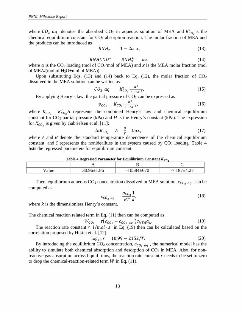
As shown in Figure 4, if CO2 loading exceeds 0.4, 𝑃𝑃∗ may vary significantly for a small change in loading [6]. This makes the measurement of 𝑃𝑃∗ important for determining the log mean driving force.
Figure 4 P* versus CO2 Loading
Table 3 depicts the data for CO2-related measurements. The orange cells indicate the targeted test conditions. The teal cells provide the actual delivered flow based on the mass flow controller calibrations. These are quite close to the targeted flows and are provided so that the model validation can employ the most accurate value available. Included is a column for the 𝑃𝑃∗ used in calculating the driving force. Two approaches are engaged to determine the 𝑃𝑃∗ to be used in calculating the driving force. For solution loadings and temperatures that were expected to produce a 𝑃𝑃∗ less than 1.5% of the pressure in the gas phase, the 𝑃𝑃∗ value is zero. This could result in a small overestimate of the driving force, which would bias the overall mass transfer coefficient low by up to 1.5%. However, this level of error was deemed to be within our experimental accuracy. If the 𝑃𝑃∗ is expected to be more than 1.5% of the overall driving force, then three points are taken, and the x-axis intercept of a linear fit of the plot of flux versus CO2 pressure is used to estimate 𝑃𝑃∗. The 𝑃𝑃∗ is taking into account for run No. 26-28, 33-35, 40, 41, 48, 49, and 52.

PNNL Milestone Report
11
Table 3 CO2/MEA Experimental Data
3. Numerical Modeling of WWC 3.1 General Theory on Mass Transport and Chemistry A volume of fluid (VOF) model is employed to solve for two Newtonian, incompressible, isothermal, and immiscible fluid flows by tracking the volume fraction (𝛼𝛼𝑖𝑖) of each phase (the subscript i = L or g stands for liquid or gas phase) in the volume fraction equation. The volume fraction equation is introduced as 𝜕𝜕
𝜕𝜕𝑜𝑜(𝛼𝛼𝐿𝐿) + ∇ ∙ (𝛼𝛼𝐿𝐿𝒖𝒖) = 0, (3)
where 𝒖𝒖 = (𝑢𝑢, 𝑣𝑣,𝑤𝑤) denotes the velocity in x, y, and z direction, respectively. The volume fraction of gas phase 𝛼𝛼𝑔𝑔 can be computed as 𝛼𝛼𝑔𝑔 = 1 − 𝛼𝛼𝐿𝐿. (4) The continuity and Navier-Stokes equations are given by 𝜕𝜕𝜕𝜕
𝜕𝜕𝑜𝑜+ ∇ ∙ (𝜌𝜌𝒖𝒖) = 0, (5)
𝜕𝜕𝜕𝜕𝑜𝑜
(𝜌𝜌𝒖𝒖) + ∇ ∙ (𝜌𝜌𝒖𝒖𝒖𝒖) = −∇p + ∇ ∙ [𝜇𝜇(∇𝒖𝒖+ ∇𝒖𝒖𝑇𝑇)] + 𝜌𝜌𝒈𝒈 − 𝑭𝑭𝑠𝑠𝑜𝑜, (6) where density 𝜌𝜌 and viscosity 𝜇𝜇 can be defined by a volume fraction averaged form as 𝜌𝜌 = 𝛼𝛼𝐿𝐿𝜌𝜌𝐿𝐿 + 𝛼𝛼𝑔𝑔𝜌𝜌𝑔𝑔, (7) 𝜇𝜇 = 𝛼𝛼𝐿𝐿𝜇𝜇𝐿𝐿 + 𝛼𝛼𝑔𝑔𝜇𝜇𝑔𝑔. (8) The surface tension force, 𝑭𝑭𝑠𝑠𝑜𝑜 in Eq. (4) can be expressed using the continuum surface force (CSF) model proposed by Brackbill et al. [7]: 𝑭𝑭𝑠𝑠𝑜𝑜 = 𝜎𝜎𝑠𝑠𝑠𝑠𝜕𝜕𝜌𝜌∇𝛼𝛼𝐿𝐿
2 �𝜕𝜕𝐿𝐿+𝜕𝜕𝑔𝑔�, (9)
Summary Table -All CO2 data Rev 2 Corrections in Yel low
Run#
MEA_content, (mass fraction MEA with water)
CO2_Loading, (mol CO2 per mol MEA)
Solvent_Flow_Rate
Gas_Flow_Rate, sccm (Includes N2 and CO2 but not water vapor added to gas before entering column)
CO2_Molar_Conc (mole fraction CO2 in gas entering column prior to humidification)
As Del ivered, Gas Flow tota l (N2+CO2)
As del ivered CO2 molar fraction (dry)
Temperature, C
P_CO2_in P_CO2_outP* used in LMPD Calc
LMPD N_CO2 KG
mass fraction mol/mol cc/min sccm mol fraction [sccm] mol fraction °C [Pa] [Pa] [Pa] [Pa] [mol/m2/s] [mol/m2/s/Pa]Run_21 0.25 0.30 450 4000 0.115 3959 0.1149 42 1.07E+04 9.14E+03 0 9.87E+03 1.30E-02 1.32E-06Run_22 0.10 0.10 495 4344 0.070 4295 0.0695 45 6.36E+03 5.37E+03 0 5.85E+03 9.17E-03 1.57E-06Run_23 0.10 0.20 590 2126 0.191 2083 0.1923 27 1.85E+04 1.55E+04 0 1.70E+04 1.47E-02 8.64E-07Run_24 0.10 0.20 352 2724 0.086 2678 0.0855 49 7.58E+03 6.31E+03 0 6.92E+03 7.71E-03 1.11E-06Run_25 0.10 0.30 550 2558 0.164 2520 0.1643 55 1.39E+04 1.21E+04 0 1.30E+04 1.13E-02 8.69E-07Run_26 0.10 0.40 318 2284 0.183 2240 0.1841 47 1.64E+04 1.48E+04 1.18E+03 1.44E+04 8.71E-03 6.04E-07Run_27 0.10 0.40 404 3474 0.158 3426 0.1587 59 1.28E+04 1.23E+04 6.14E+03 6.42E+03 4.46E-03 6.94E-07Run_28 0.10 0.50 558 2681 0.056 2634 0.0550 32 5.23E+03 5.02E+03 1.39E+03 3.73E+03 1.10E-03 2.95E-07Run_29 0.20 0.10 322 2342 0.032 2304 0.0301 30 2.87E+03 2.18E+03 0 2.51E+03 3.19E-03 1.27E-06Run_30 0.20 0.20 426 3735 0.142 3694 0.1420 31 1.35E+04 1.15E+04 0 1.25E+04 1.65E-02 1.32E-06Run_31 0.20 0.20 466 3899 0.064 3857 0.0632 38 5.89E+03 4.92E+03 0 5.39E+03 7.69E-03 1.43E-06Run_32 0.20 0.30 338 5549 0.134 5503 0.1341 53 1.16E+04 1.06E+04 0 1.11E+04 1.43E-02 1.29E-06Run_33 0.20 0.40 410 3345 0.127 3300 0.1270 43 1.17E+04 1.07E+04 7.24E+02 1.05E+04 7.37E-03 7.06E-07Run_34 0.20 0.40 475 3635 0.043 3598 0.0421 56 3.56E+03 3.51E+03 3.09E+03 4.42E+02 3.86E-04 8.74E-07Run_35 0.20 0.50 521 2861 0.147 2816 0.1475 39 1.38E+04 1.32E+04 2.45E+03 1.10E+04 3.92E-03 3.56E-07Run_36 0.30 0.10 363 4682 0.106 4636 0.1059 41 9.88E+03 8.04E+03 0 8.93E+03 1.85E-02 2.08E-06Run_37 0.30 0.20 532 5130 0.175 5085 0.1753 33 1.68E+04 1.48E+04 0 1.57E+04 2.41E-02 1.53E-06Run_38 0.30 0.20 375 5241 0.049 5195 0.0486 56 4.14E+03 3.49E+03 0 3.80E+03 7.77E-03 2.04E-06Run_39 0.30 0.30 488 3107 0.110 3062 0.1098 52 9.61E+03 7.99E+03 0 8.77E+03 1.16E-02 1.33E-06Run_40 0.30 0.40 432 4189 0.102 4144 0.1018 41 9.46E+03 8.65E+03 -8.20E+00 9.05E+03 7.40E-03 8.17E-07Run_41 0.30 0.40 458 4839 0.079 4799 0.0785 51 6.95E+03 6.46E+03 1.17E+03 5.54E+03 5.34E-03 9.64E-07Run_42 0.30 0.50 308 5991 0.196 5942 0.1966 25 1.92E+04 1.89E+04 0 1.90E+04 5.04E-03 2.65E-07Run_43 0.40 0.10 537 4431 0.116 4386 0.1158 46 1.06E+04 8.23E+03 0 9.36E+03 2.33E-02 2.49E-06Run_44 0.40 0.20 513 4066 0.121 4020 0.1211 36 1.15E+04 9.54E+03 0 1.05E+04 1.69E-02 1.61E-06Run_45 0.40 0.20 570 5673 0.179 5628 0.1794 59 1.52E+04 1.29E+04 0 1.40E+04 3.31E-02 2.36E-06Run_46 0.40 0.30 378 5301 0.040 5259 0.0393 34 3.76E+03 3.39E+03 0 3.57E+03 4.02E-03 1.13E-06Run_47 0.40 0.40 588 5790 0.093 5742 0.0929 28 9.05E+03 8.51E+03 0 8.78E+03 6.44E-03 7.34E-07Run_48 0.40 0.40 449 4869 0.153 4825 0.1532 49 1.39E+04 1.28E+04 5.35E+02 1.28E+04 1.27E-02 9.93E-07Run_49 0.40 0.50 395 3189 0.078 3145 0.0774 37 7.36E+03 7.07E+03 1.84E+03 5.38E+03 1.74E-03 3.23E-07Run_50 0.25 0.30 450 4000 0.115 3959 0.1149 42 1.06E+04 9.15E+03 0 9.87E+03 1.30E-02 1.31E-06Run_51 0.10 0.20 590 2126 0.191 2083 0.1923 27 1.85E+04 1.52E+04 0 1.68E+04 1.58E-02 9.41E-07Run_52 0.40 0.40 449 4869 0.153 4823 0.1532 49 1.38E+04 1.27E+04 5.67E+01 1.32E+04 1.34E-02 1.01E-06
orange headers indicate the input values that defined the test to be run

PNNL Milestone Report
12
where 𝜎𝜎𝑠𝑠𝑜𝑜 is the surface tension coefficient, 𝜅𝜅 = −∇ ∙ 𝒏𝒏� represents the curvature of the surface, and 𝒏𝒏� is the unit interface normal vector, which can be defined as 𝒏𝒏� = 𝒏𝒏
|𝒏𝒏|, (10) where 𝒏𝒏 = �𝑙𝑙𝑥𝑥, 𝑙𝑙𝑦𝑦,𝑙𝑙𝑧𝑧� = −∇𝛼𝛼𝐿𝐿 is the vector along the interface normal. The one-fluid equation [8] considering convection, diffusion, interface mass transport, and chemical reactions will be implemented to calculate gas concentration in both phases by using only one equation for the entire domain: 𝜕𝜕𝑐𝑐𝑖𝑖
𝜕𝜕𝑜𝑜+ ∇ ∙ (𝒖𝒖𝑐𝑐𝑖𝑖 − D𝑖𝑖∇𝑐𝑐𝑖𝑖 − Γ𝑖𝑖) −𝑊𝑊𝑖𝑖 = 0, (11)
where Γ𝑖𝑖 = −D𝑖𝑖
𝑐𝑐𝑖𝑖(1−𝑘𝑘𝑖𝑖)𝛼𝛼𝐿𝐿+𝑘𝑘𝑖𝑖(1−𝛼𝛼𝐿𝐿)∇𝛼𝛼𝐿𝐿,
𝐷𝐷𝑖𝑖 = 𝐷𝐷𝑖𝑖,𝐿𝐿𝐷𝐷𝑖𝑖.𝑔𝑔𝛼𝛼𝐿𝐿𝐷𝐷𝑖𝑖,𝑔𝑔+(1−𝛼𝛼𝐿𝐿)𝐷𝐷𝑖𝑖,𝐿𝐿
.
Here, 𝑐𝑐𝑖𝑖 represents the concentration for species 𝑖𝑖. The diffusivity 𝐷𝐷𝑖𝑖 is computed by the harmonic interpolation, 𝑘𝑘𝑖𝑖 = 𝑐𝑐𝑖𝑖,𝑔𝑔𝐼𝐼 /𝑐𝑐𝑖𝑖,𝐿𝐿𝐼𝐼 denotes the dimensionless Henry’s constant, where 𝑐𝑐𝑖𝑖,𝑔𝑔𝐼𝐼 and 𝑐𝑐𝑖𝑖,𝐿𝐿𝐼𝐼 are the gas phase and liquid phase concentration of species 𝑖𝑖 at the gas-liquid interface. Please note that the concentration of any species in gas and liquid phase normally has a discontinuity across the interface because of the different solubility in each phase. The term 𝛤𝛤 in Eq. (11) accounts for this discontinuity unless 𝛤𝛤 approaches zero for 𝑘𝑘𝑖𝑖 =1 (same solubility in both phases). The last term 𝑊𝑊𝑖𝑖 is the production term is related to the chemical reaction. The chemical reactions of CO2 absorption by MEA have been extensively investigated and three sub-reactions indicate vital influence on the CO2/MEA reaction [9, 10]. They can be expressed as: Carbamate formation: 𝐶𝐶𝑂𝑂2 + 2𝑅𝑅𝑅𝑅𝐻𝐻2 → 𝑅𝑅𝑅𝑅𝐻𝐻𝐶𝐶𝑂𝑂𝑂𝑂− + 𝑅𝑅𝑅𝑅𝐻𝐻3+ Bicarbonate formation: 𝐶𝐶𝑂𝑂2 + 𝑅𝑅𝑅𝑅𝐻𝐻2 + 𝐻𝐻2𝑂𝑂 → 𝐻𝐻𝐶𝐶𝑂𝑂3− + 𝑅𝑅𝑅𝑅𝐻𝐻3+ Carbamate reversion: 𝑅𝑅𝑅𝑅𝐻𝐻𝐶𝐶𝑂𝑂𝑂𝑂− + 𝐶𝐶𝑂𝑂2 + 2𝐻𝐻2𝑂𝑂 → 𝐻𝐻𝐶𝐶𝑂𝑂3− + 2𝑅𝑅𝑅𝑅𝐻𝐻3+, where 𝑅𝑅 = 𝐶𝐶𝐻𝐻2𝐶𝐶𝐻𝐻2𝑂𝑂𝐻𝐻. It is suggested by Astarita et al. [9] that the rate of bicarbonate formation is negligible because of MEA carbamate’s high stability. In addition, the overall absorption rate can be approximated as irreversible, making the carbamate reversion insignificant. As a result, the overall CO2/MEA reaction rate will dominate by the carbamate formation. When chemical equilibrium state is reached in the liquid phase, the chemical equilibrium reaction and equilibrium constant of the carbamate formation can be written as
𝑅𝑅𝑅𝑅𝐻𝐻𝐶𝐶𝑂𝑂𝑂𝑂− + 𝑅𝑅𝑅𝑅𝐻𝐻3+𝐾𝐾𝐶𝐶𝑂𝑂2′
��� 𝐶𝐶𝑂𝑂2(𝑎𝑎𝑎𝑎) + 2𝑅𝑅𝑅𝑅𝐻𝐻2
𝐾𝐾𝐶𝐶𝑂𝑂2′ =
[𝐶𝐶𝑂𝑂2(𝑎𝑎𝑎𝑎)][𝑅𝑅𝑅𝑅𝐻𝐻2]2
[𝑅𝑅𝑅𝑅𝐻𝐻𝐶𝐶𝑂𝑂𝑂𝑂−][𝑅𝑅𝑅𝑅𝐻𝐻3+], (12)
PNNL Milestone Report
13
where 𝐶𝐶𝑂𝑂2(𝑎𝑎𝑎𝑎) denotes the absorbed CO2 in aqueous solution of MEA and 𝐾𝐾𝐶𝐶𝑂𝑂2′ is the
chemical equilibrium constant for CO2 absorption reaction. The molar fraction of MEA and the products can be introduced as [𝑅𝑅𝑅𝑅𝐻𝐻2] = (1 − 2𝛼𝛼)𝑥𝑥, (13) [𝑅𝑅𝑅𝑅𝐻𝐻𝐶𝐶𝑂𝑂𝑂𝑂−] = [𝑅𝑅𝑅𝑅𝐻𝐻3+] = 𝛼𝛼𝑥𝑥, (14) where 𝛼𝛼 is the CO2 loading (mol of CO2/mol of MEA) and 𝑥𝑥 is the MEA molar fraction (mol of MEA/(mol of H2O+mol of MEA)). Upon substituting Eqs. (13) and (14) back to Eq. (12), the molar fraction of CO2 dissolved in the MEA solution can be written as [𝐶𝐶𝑂𝑂2(𝑎𝑎𝑎𝑎)] = 𝐾𝐾𝐶𝐶𝑂𝑂2
′ 𝛼𝛼2
(1−2𝛼𝛼)2. (15) By applying Henry’s law, the partial pressure of CO2 can be expressed as 𝑝𝑝𝐶𝐶𝑂𝑂2 = 𝐾𝐾𝐶𝐶𝑂𝑂2
𝛼𝛼2
(1−2𝛼𝛼)2, (16) where 𝐾𝐾𝐶𝐶𝑂𝑂2 = 𝐾𝐾𝐶𝐶𝑂𝑂2
′ 𝐻𝐻 represents the combined Henry’s law and chemical equilibrium constant for CO2 partial pressure (kPa) and H is the Henry’s constant (kPa). The expression for 𝐾𝐾𝐶𝐶𝑂𝑂2 is given by Gabrielsen et al. [11]: 𝑙𝑙𝑙𝑙𝐾𝐾𝐶𝐶𝑂𝑂2 = 𝐴𝐴 + 𝐵𝐵
𝑇𝑇+ 𝐶𝐶𝛼𝛼𝑥𝑥, (17)
where 𝐴𝐴 and 𝐵𝐵 denote the standard temperature dependence of the chemical equilibrium constant, and 𝐶𝐶 represents the nonidealities in the system caused by CO2 loading. Table 4 lists the regressed parameters for equilibrium constant.
Table 4 Regressed Parameter for Equilibrium Constant 𝑲𝑲𝑲𝑲𝑲𝑲𝟐𝟐 A B C
Value 30.96±1.86 -10584±670 -7.187±4.27 Then, equilibrium aqueous CO2 concentration dissolved in MEA solution, 𝑐𝑐𝐶𝐶𝑂𝑂2(𝑎𝑎𝑎𝑎) can be computed as
𝑐𝑐𝐶𝐶𝑂𝑂2(𝑎𝑎𝑎𝑎) =𝑝𝑝𝐶𝐶𝑂𝑂2𝑅𝑅𝑅𝑅
1𝑘𝑘
, (18)
where 𝑘𝑘 is the dimensionless Henry’s constant. The chemical reaction related term in Eq. (11) then can be computed as 𝑊𝑊𝐶𝐶𝑂𝑂2 = r�𝑐𝑐𝐶𝐶𝑂𝑂2 − 𝑐𝑐𝐶𝐶𝑂𝑂2(𝑎𝑎𝑎𝑎)�𝑐𝑐𝑀𝑀𝑀𝑀𝑀𝑀𝛼𝛼𝐿𝐿 . (19) The reaction rate constant 𝑟𝑟 (𝑙𝑙/𝑚𝑚𝑚𝑚𝑙𝑙 ∙ 𝑠𝑠) in Eq. (19) then can be calculated based on the correlation proposed by Hikita et al. [12]: log10 𝑟𝑟 = 10.99 − 2152/𝑅𝑅. (20) By introducing the equilibrium CO2 concentration, 𝑐𝑐𝐶𝐶𝑂𝑂2(𝑎𝑎𝑎𝑎), the numerical model has the ability to simulate both chemical absorption and desorption of CO2 in MEA. Also, for non-reactive gas absorption across liquid films, the reaction rate constant 𝑟𝑟 needs to be set to zero to drop the chemical-reaction-related term 𝑊𝑊 in Eq. (11).
PNNL Milestone Report
14
3.2 Calculation of Model Input Parameters The input parameters used in the CFD modeling include MEA solvent density, MEA solvent kinematic viscosity, gas diffusivity in solvent, gas Henry’s constant in solvent, MEA diffusivity in solvent, gas density, gas dynamics viscosity, gas diffusivity, and surface tension. The values of these parameters are taken from literature.
3.2.1 MEA Solvent Density MEA solution density is calculated by the average molecular weight divided by its overall molar volume. 𝜌𝜌𝑠𝑠𝑜𝑜𝑠𝑠𝑠𝑠𝑠𝑠𝑖𝑖𝑜𝑜 = 𝑥𝑥𝑀𝑀𝑀𝑀𝑀𝑀𝑀𝑀𝑀𝑀𝑀𝑀𝑀𝑀+𝑥𝑥𝐻𝐻2𝑂𝑂𝑀𝑀𝐻𝐻2𝑂𝑂+𝑥𝑥𝐶𝐶𝑂𝑂2𝑀𝑀𝐶𝐶𝑂𝑂2
𝑉𝑉, (21)
where 𝜌𝜌𝑠𝑠𝑜𝑜𝑠𝑠𝑠𝑠𝑠𝑠𝑖𝑖𝑜𝑜 is solvent density (𝑔𝑔/𝑚𝑚𝑚𝑚), 𝑉𝑉 is molar volume of the solvent (𝑚𝑚𝑚𝑚/𝑚𝑚𝑚𝑚𝑙𝑙), 𝑥𝑥 is molar fraction, and 𝑀𝑀 is molecular weight (𝑔𝑔/𝑚𝑚𝑚𝑚𝑙𝑙). The solvent’s molar volume can be expressed as [3]: 𝑉𝑉 = 𝑥𝑥𝑀𝑀𝑀𝑀𝑀𝑀𝑉𝑉𝑀𝑀𝑀𝑀𝑀𝑀 + 𝑥𝑥𝐻𝐻2𝑂𝑂𝑉𝑉𝐻𝐻2𝑂𝑂 + 𝑥𝑥𝐶𝐶𝑂𝑂2𝑉𝑉𝐶𝐶𝑂𝑂2 + 𝑥𝑥𝑀𝑀𝑀𝑀𝑀𝑀𝑥𝑥𝐻𝐻2𝑂𝑂𝑉𝑉
∗, (22) where
𝑉𝑉𝑀𝑀𝑀𝑀𝑀𝑀 =𝑀𝑀𝑀𝑀𝑀𝑀𝑀𝑀
𝑎𝑎𝑅𝑅2 + 𝑏𝑏𝑅𝑅 + 𝑐𝑐.
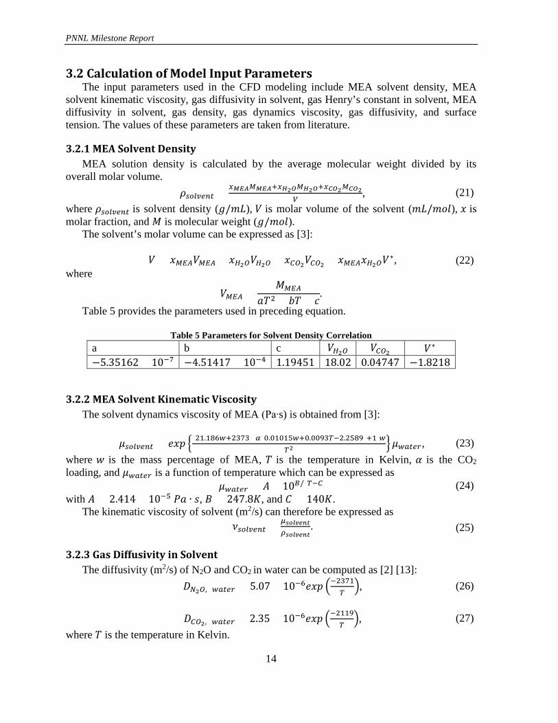
Table 5 provides the parameters used in preceding equation.
Table 5 Parameters for Solvent Density Correlation a b c 𝑉𝑉𝐻𝐻2𝑂𝑂 𝑉𝑉𝐶𝐶𝑂𝑂2 𝑉𝑉∗ −5.35162 × 10⁻⁷ −4.51417 × 10⁻⁴ 1.19451 18.02 0.04747 −1.8218
3.2.2 MEA Solvent Kinematic Viscosity The solvent dynamics viscosity of MEA (Pa∙s) is obtained from [3]: 𝜇𝜇𝑠𝑠𝑜𝑜𝑠𝑠𝑠𝑠𝑠𝑠𝑖𝑖𝑜𝑜 = 𝑒𝑒𝑥𝑥𝑝𝑝 �(21.186𝑤𝑤+2373)[𝛼𝛼(0.01015𝑤𝑤+0.0093𝑇𝑇−2.2589)+1]𝑤𝑤
𝑇𝑇2� 𝜇𝜇𝑤𝑤𝑎𝑎𝑜𝑜𝑠𝑠𝑤𝑤, (23)
where 𝑤𝑤 is the mass percentage of MEA, 𝑅𝑅 is the temperature in Kelvin, 𝛼𝛼 is the CO2 loading, and 𝜇𝜇𝑤𝑤𝑎𝑎𝑜𝑜𝑠𝑠𝑤𝑤 is a function of temperature which can be expressed as 𝜇𝜇𝑤𝑤𝑎𝑎𝑜𝑜𝑠𝑠𝑤𝑤 = 𝐴𝐴 × 10𝐵𝐵/(𝑇𝑇−𝐶𝐶) (24) with 𝐴𝐴 = 2.414 × 10⁻⁵ 𝑃𝑃𝑎𝑎 ∙ 𝑠𝑠, 𝐵𝐵 = 247.8𝐾𝐾, and 𝐶𝐶 = 140𝐾𝐾. The kinematic viscosity of solvent (m2/s) can therefore be expressed as 𝜈𝜈𝑠𝑠𝑜𝑜𝑠𝑠𝑠𝑠𝑠𝑠𝑖𝑖𝑜𝑜 = 𝜇𝜇𝑠𝑠𝑠𝑠𝑠𝑠𝑠𝑠𝑠𝑠𝑠𝑠𝑠𝑠
𝜕𝜕𝑠𝑠𝑠𝑠𝑠𝑠𝑠𝑠𝑠𝑠𝑠𝑠𝑠𝑠. (25)
3.2.3 Gas Diffusivity in Solvent The diffusivity (m2/s) of N2O and CO2 in water can be computed as [2] [13]: 𝐷𝐷𝑁𝑁2𝑂𝑂, 𝑤𝑤𝑎𝑎𝑜𝑜𝑠𝑠𝑤𝑤 = 5.07 × 10⁻⁶𝑒𝑒𝑥𝑥𝑝𝑝 �−2371
𝑇𝑇�, (26)
𝐷𝐷𝐶𝐶𝑂𝑂2, 𝑤𝑤𝑎𝑎𝑜𝑜𝑠𝑠𝑤𝑤 = 2.35 × 10⁻⁶𝑒𝑒𝑥𝑥𝑝𝑝 �−2119
𝑇𝑇�, (27)
where 𝑅𝑅 is the temperature in Kelvin.

PNNL Milestone Report
15
The diffusivity of CO2 in MEA solution can be computed as [13]: 𝐷𝐷𝐶𝐶𝑂𝑂2, 𝑀𝑀𝑀𝑀𝑀𝑀 = 𝐷𝐷𝐶𝐶𝑂𝑂2, 𝑤𝑤𝑎𝑎𝑜𝑜𝑠𝑠𝑤𝑤 �
𝜇𝜇𝑤𝑤𝑤𝑤𝑠𝑠𝑠𝑠𝑤𝑤𝜇𝜇𝑠𝑠𝑠𝑠𝑠𝑠𝑠𝑠𝑠𝑠𝑠𝑠𝑠𝑠
�0.8
. (28)
The diffusivity of N2O in MEA solution can be computed as [2]: 𝐷𝐷𝑁𝑁2𝑂𝑂, 𝑀𝑀𝑀𝑀𝑀𝑀 = 𝐷𝐷𝐶𝐶𝑂𝑂2, 𝑀𝑀𝑀𝑀𝑀𝑀
𝐷𝐷𝑁𝑁2𝑂𝑂, 𝑤𝑤𝑤𝑤𝑠𝑠𝑠𝑠𝑤𝑤
𝐷𝐷𝐶𝐶𝑂𝑂2, 𝑤𝑤𝑤𝑤𝑠𝑠𝑠𝑠𝑤𝑤. (29)
3.2.4 Gas Henry’s Constant in Solvent The dimensionless Henry’s constant of N2O and CO2 in water can be computed as [2] [13]:
𝐻𝐻𝑁𝑁2𝑂𝑂, 𝑤𝑤𝑎𝑎𝑜𝑜𝑠𝑠𝑤𝑤 = 𝑅𝑅𝑅𝑅/8.5470 × 10−6𝑒𝑒𝑥𝑥𝑝𝑝 �−2284𝑅𝑅
� (30)
𝐻𝐻𝐶𝐶𝑂𝑂2, 𝑤𝑤𝑎𝑎𝑜𝑜𝑠𝑠𝑤𝑤 = 𝑅𝑅𝑅𝑅/2.8249 × 10−6𝑒𝑒𝑥𝑥𝑝𝑝 �−2044
𝑇𝑇�, (31)
where 𝑅𝑅 is the ideal gas constant (𝐽𝐽/𝐾𝐾 ∙ 𝑚𝑚𝑚𝑚𝑙𝑙) and 𝑅𝑅 is the temperature (K). The dimensionless Henry’s constant of CO2 in MEA solution can be computed as [13]: 𝐻𝐻𝐶𝐶𝑂𝑂2, 𝑀𝑀𝑀𝑀𝑀𝑀 = 0.01𝑅𝑅𝑅𝑅/10(5.3−0.035𝑐𝑐𝑀𝑀𝑀𝑀𝑀𝑀−1140/𝑇𝑇), (32) where 𝑐𝑐𝑀𝑀𝑀𝑀𝑀𝑀 is the MEA molar concentration (mol/m3). The dimensionless Henry’s constant of N2O in MEA solution can be computed as [2]:
𝐻𝐻𝑁𝑁2𝑂𝑂, 𝑀𝑀𝑀𝑀𝑀𝑀 = 𝐻𝐻𝐶𝐶𝑂𝑂2, 𝑀𝑀𝑀𝑀𝑀𝑀𝐻𝐻𝑁𝑁2𝑂𝑂, 𝑤𝑤𝑎𝑎𝑜𝑜𝑠𝑠𝑤𝑤
𝐻𝐻𝐶𝐶𝑂𝑂2, 𝑤𝑤𝑎𝑎𝑜𝑜𝑠𝑠𝑤𝑤. (33)
3.2.5 MEA Diffusivity in Solvent The diffusivity of MEA in solvent (m2/s) with the operative range of the temperature and MEA concentration can be described as [14]: ln(𝐷𝐷𝑀𝑀𝑀𝑀𝑀𝑀) = −13.275 − 2198.3
𝑇𝑇− 7.8142𝑒𝑒−5𝑐𝑐, (34)
where
43 < 𝑐𝑐 < 5016𝑚𝑚𝑚𝑚𝑙𝑙/𝑚𝑚3, 298 < 𝑅𝑅 < 333𝐾𝐾.
3.2.6 Gas Density Assuming the gas input into the domain is a gas mixture, the mixture’s density (kg/m3) can be expressed as 𝜌𝜌𝑔𝑔𝑎𝑎𝑠𝑠 = 𝑐𝑐𝑖𝑖
𝑥𝑥𝑖𝑖∑ 𝑥𝑥𝑖𝑖𝑀𝑀𝑖𝑖, (35)
where 𝑥𝑥𝑖𝑖 is the molar fraction of the species 𝑖𝑖, 𝑐𝑐𝑖𝑖 is the molar concentration (mol/m3), and 𝑀𝑀𝑖𝑖 is the molar mass (kg/mol).
3.2.7 Gas Dynamics Viscosity For a multicomponent gas system, the general dynamics viscosity (Pa∙s) can be expressed as [15]:

PNNL Milestone Report
16
𝜇𝜇𝑔𝑔𝑎𝑎𝑠𝑠 = ∑ 𝜇𝜇𝑖𝑖1+ 1
𝑥𝑥𝑖𝑖∑ 𝑥𝑥𝑗𝑗𝜙𝜙𝑖𝑖𝑗𝑗𝑠𝑠𝑗𝑗=1𝑗𝑗≠𝑖𝑖
𝑖𝑖𝑖𝑖=1 , (36)
where
𝜙𝜙𝑖𝑖𝑖𝑖 =�1+(𝜇𝜇𝑖𝑖/𝜇𝜇𝑗𝑗)1/2�𝑀𝑀𝑖𝑖/𝑀𝑀𝑗𝑗�
1/4�2
4√2�1+�𝑀𝑀𝑖𝑖/𝑀𝑀𝑗𝑗��1/2 ,
𝑥𝑥 is the molar fraction of, 𝜇𝜇 is dynamics viscosity (Pa∙s), and 𝑀𝑀 is molar mass (g/mol).
3.2.8 Gas Diffusivity The binary diffusion coefficient can be determined from the Chapman-Enskog theory [16]:
𝐷𝐷i,j = 0.0018583 � 1𝑀𝑀𝑖𝑖
+ 1𝑀𝑀𝑗𝑗�1/2 𝑇𝑇2/3
𝑃𝑃𝜖𝜖i,j2 Ω𝐷𝐷
, (37)
where 𝑀𝑀 is molar weight (g/mol), 𝑃𝑃 is pressure (atm), 𝜖𝜖i,j is the collision diameter in Å, and Ω𝐷𝐷 is collision integral. The equations for calculating 𝜖𝜖i,j and Ω𝐷𝐷 can be expressed as
𝜖𝜖i,j = 𝜖𝜖i+𝜖𝜖j2
,
Ω𝐷𝐷 = 1.06𝑜𝑜0.156 + 0.193
exp (0.476𝑜𝑜)+ 1.036
exp (1.53𝑜𝑜)+ 1.765
3.894t,
where t is determined by t = kBT
ξi,j.
The Boltzmann constant kB=1.38066×10⁻²³(J·K-1), and ξi,j is the Lennard-Jones potential energy function that can be expressed as ξi,j = �ξiξj.
Table 6 includes listed 𝜖𝜖i and ξi/kB values for several commonly used gases [16].
Table 6 𝛔𝛔𝛔𝛔 and 𝛏𝛏𝛔𝛔/𝐤𝐤𝐤𝐤 Values N2 O2 CH4 H2O CO H2 CO2
𝜖𝜖i 3.798 3.467 3.758 2.641 3.69 2.827 3.941 ξi/kB 71.4 106.7 148.6 809.1 91.7 59.7 195.2
3.2.9 Surface Tension The surface tension (kg/s2) of MEA solution can be expressed as [17]:
𝜎𝜎 = 𝑥𝑥𝐻𝐻2𝑂𝑂𝜎𝜎𝐻𝐻2𝑂𝑂 + 𝑥𝑥𝑀𝑀𝑀𝑀𝑀𝑀𝜎𝜎𝑀𝑀𝑀𝑀𝑀𝑀 + [−0.567 + 1.05𝑤𝑤𝑀𝑀𝑀𝑀𝑀𝑀 −0.552𝑤𝑤𝑀𝑀𝑀𝑀𝑀𝑀
2 ]𝑅𝑅𝑥𝑥𝐻𝐻2𝑂𝑂𝑥𝑥𝑀𝑀𝑀𝑀𝑀𝑀 + �6175.83𝑤𝑤𝑤𝑤𝑠𝑠𝑟𝑟1 + 2828.87𝑤𝑤𝑤𝑤𝑠𝑠𝑟𝑟12 �/𝑅𝑅 +
27494.72𝛼𝛼𝑤𝑤𝑤𝑤𝑠𝑠𝑟𝑟2/𝑅𝑅, (38)
PNNL Milestone Report
17
where
𝑤𝑤𝑤𝑤𝑠𝑠𝑟𝑟1 =𝛼𝛼𝑤𝑤𝑀𝑀𝑀𝑀𝑀𝑀𝑀𝑀𝐶𝐶𝑂𝑂2
𝑀𝑀𝑀𝑀𝑀𝑀𝑀𝑀+𝛼𝛼𝑤𝑤𝑀𝑀𝑀𝑀𝑀𝑀/𝛼𝛼𝑚𝑚𝑤𝑤𝑥𝑥
1+𝛼𝛼𝑤𝑤𝑀𝑀𝑀𝑀𝑀𝑀𝑀𝑀𝐶𝐶𝑂𝑂2
𝑀𝑀𝑀𝑀𝑀𝑀𝑀𝑀
,
𝑤𝑤𝑤𝑤𝑠𝑠𝑟𝑟2 = 1−𝛼𝛼/𝛼𝛼𝑚𝑚𝑤𝑤𝑥𝑥
1+𝛼𝛼𝑤𝑤𝑀𝑀𝑀𝑀𝑀𝑀𝑀𝑀𝐶𝐶𝑂𝑂2
𝑀𝑀𝑀𝑀𝑀𝑀𝑀𝑀
,
𝑤𝑤 is mass fraction, 𝑥𝑥 is molar fraction, 𝛼𝛼 is CO2 loading, 𝑅𝑅 is operating temperature (K), 𝑀𝑀 is molar mass (g/mol), 𝜎𝜎𝑖𝑖 is the surface tension of pure component 𝑖𝑖 at operating temperature, and 𝛼𝛼𝑚𝑚𝑎𝑎𝑥𝑥 is the maximum CO2 loading. 𝛼𝛼𝑚𝑚𝑎𝑎𝑥𝑥 is a function of both temperature and MEA mass fraction, and the value of 𝛼𝛼𝑚𝑚𝑎𝑎𝑥𝑥 can be found in [17]. 3.3 CFD Model Setup
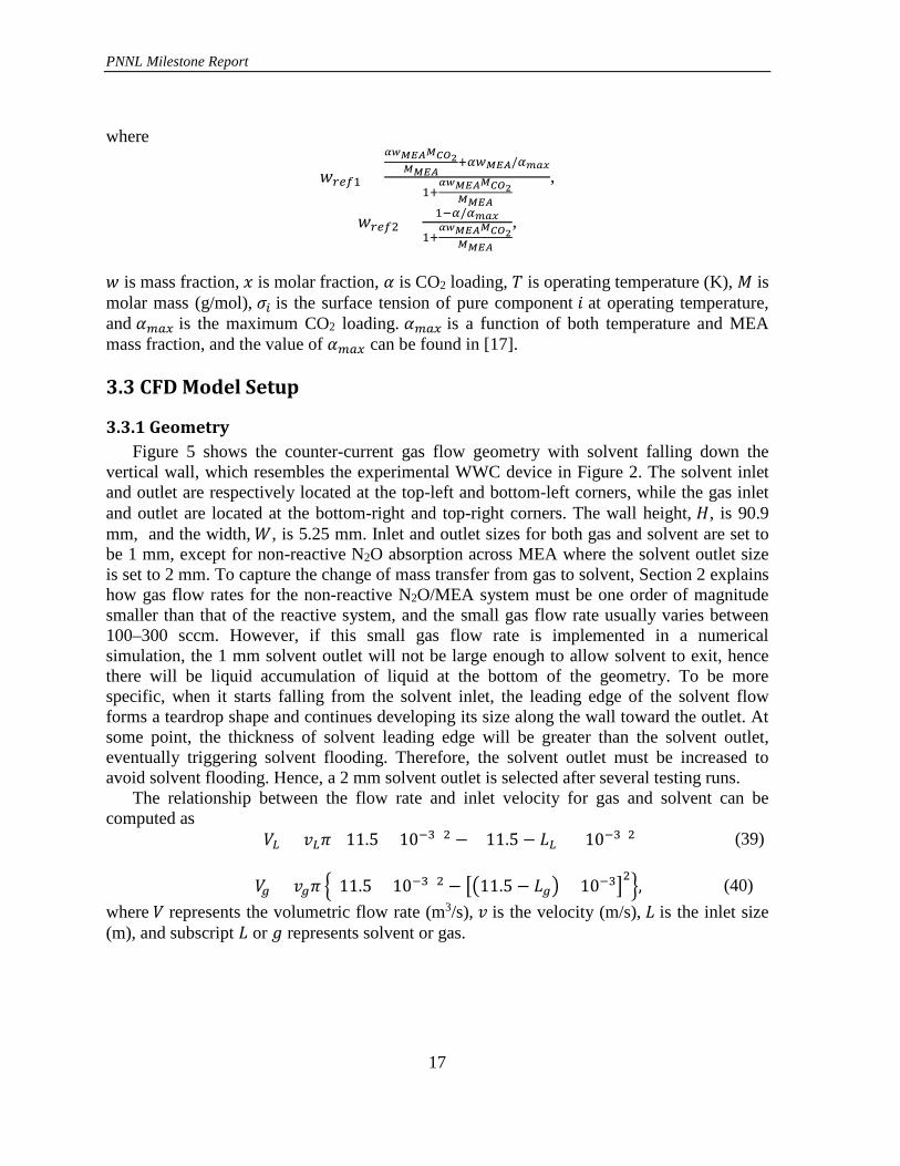
3.3.1 Geometry Figure 5 shows the counter-current gas flow geometry with solvent falling down the vertical wall, which resembles the experimental WWC device in Figure 2. The solvent inlet and outlet are respectively located at the top-left and bottom-left corners, while the gas inlet and outlet are located at the bottom-right and top-right corners. The wall height, 𝐻𝐻, is 90.9 mm, and the width, 𝑊𝑊, is 5.25 mm. Inlet and outlet sizes for both gas and solvent are set to be 1 mm, except for non-reactive N2O absorption across MEA where the solvent outlet size is set to 2 mm. To capture the change of mass transfer from gas to solvent, Section 2 explains how gas flow rates for the non-reactive N2O/MEA system must be one order of magnitude smaller than that of the reactive system, and the small gas flow rate usually varies between 100–300 sccm. However, if this small gas flow rate is implemented in a numerical simulation, the 1 mm solvent outlet will not be large enough to allow solvent to exit, hence there will be liquid accumulation of liquid at the bottom of the geometry. To be more specific, when it starts falling from the solvent inlet, the leading edge of the solvent flow forms a teardrop shape and continues developing its size along the wall toward the outlet. At some point, the thickness of solvent leading edge will be greater than the solvent outlet, eventually triggering solvent flooding. Therefore, the solvent outlet must be increased to avoid solvent flooding. Hence, a 2 mm solvent outlet is selected after several testing runs. The relationship between the flow rate and inlet velocity for gas and solvent can be computed as 𝑉𝑉𝐿𝐿 = 𝑣𝑣𝐿𝐿𝜋𝜋{(11.5 × 10⁻³)2 − [(11.5 − 𝑚𝑚𝐿𝐿) × 10−3]2} (39) 𝑉𝑉𝑔𝑔 = 𝑣𝑣𝑔𝑔𝜋𝜋 �(11.5 × 10⁻³)2 − ��11.5 − 𝑚𝑚𝑔𝑔� × 10−3�
2�, (40)
where 𝑉𝑉 represents the volumetric flow rate (m3/s), 𝑣𝑣 is the velocity (m/s), 𝑚𝑚 is the inlet size (m), and subscript 𝑚𝑚 or 𝑔𝑔 represents solvent or gas.

PNNL Milestone Report
18
Figure 5 Countercurrent Gas Flow Geometry Schematics
3.3.2 Boundary and Initial Conditions The boundary condition for the left, right, bottom, and top walls is set to be a non-slip condition. At the solvent inlet, a laminar flow velocity, together with the concentrations of solvent species, should be given. At the solvent outlet, the mass concentration gradient (dc/dy=0) is given at zero because the flow is assumed to be fully developed [18]. For the gas inlet, concentrations of gas species, as well as gas inlet velocity, should be specified. For incompressible flow, relative pressure (pressure difference), rather than absolute pressure, is more important. Therefore, the pressure value at the gas outlet is set to zero. For initial conditions, the testing domain is placed at zero atm pressure, and the domain is filled with a given concentration of gases.
3.3.3 Input Parameters of the CFD model Table 7 lists six controlled parameters. Note that these parameters also serve as controlled operational conditions for the WWC experiments.

PNNL Milestone Report
19
Table 7 Controlled Input Parameters Parameters Unit
MEA mass fraction dimensionless
MEA CO2 loading (mol of CO2/mol of MEA)
Solvent flow rate ml/min
Gas flow rate sccm
Operating temperature °C
Gas inlet molar fraction dimensionless
For any given controlled parameters, the model input parameters listed in Table 8 can be calculated from the equations introduced in Section 3.2.
Table 8 Direct Model Input Parameters Parameters Unit
Solvent inlet velocity m/s
Gas inlet velocity m/s
Inlet concentration (solvent, gas) mol/m3
Diffusivity (solvent, gas) m2/s
Gas diffusivity in solvent m2/s
Solvent contact angle 40 (fixed)
Density (solvent, gas) kg/m3
Kinematic viscosity (solvent, gas) m2/s
Surface tension kg/s2
Henry’s constant Dimensionless
CO2 absorption rate constants l/mol·s
Equilibrium CO2 concentration mol/m3

PNNL Milestone Report
20
3.3.4 Computational Methods The multiphase flow solver InterFOAM in the OpenFOAM CFD software package is customized so that the one-fluid formulation can be solved and coupled with the continuity, momentum, and volume fraction equations. All cases are simulated until a steady-state condition is reached. A mesh sensitivity study was performed by Hu et al. [19] and Xu et al. [20]. They concluded that the mesh size of 0.1h (where h~0.4mm is the average film thickness) is sufficient to capture wave behavior of the liquid film. Based on their studies, we have adopted the mesh size to be 0.0125 mm between x = 0 and 1 mm (Figure 6, Section 1), which is ~0.035 h. As such, the simulation results are not affected by the mesh size, yet they still are computationally affordable. For x = 4.25–5.25 mm (Figure 6, Section 3), a coarse mesh size is selected to be 0.05 mm. Between x = 1 and 4.25 mm (Figure 6, Section 2), a total of 120 non-uniform mesh grids with the same expansion ratio are employed to make the ratio of the last grid to the first grid in this region equal to 4. In the y direction, a total of 1,000 grids are uniformly distributed in the domain. The maximum time step size is adjusted to be 10-5 seconds for the current simulation after several testing runs. OpenFOAM dynamically adjusts the actual time step. It takes about nine CPU hours for 16 processors to run 1 second of simulation.
Figure 6 Mesh Size Distribution in x Direction
3.4 Calculation of Overall Mass Transfer Coefficient
3.4.1 N2O/MEA System The overall mass transfer coefficient, 𝐾𝐾𝐺𝐺 (mol/Pa·s·m2) can be calculated via Eq. (1). By applying the ideal gas law, ∆𝑃𝑃 can be written as a function of temperature and N2O concentration at the gas inlet and outlet: ∆𝑃𝑃 =
�𝑐𝑐𝑁𝑁2𝑂𝑂,𝑖𝑖𝑠𝑠−𝑐𝑐𝑁𝑁2𝑂𝑂,𝑠𝑠𝑜𝑜𝑠𝑠�𝑅𝑅𝑇𝑇
𝑠𝑠𝑖𝑖�𝑐𝑐𝑁𝑁2𝑂𝑂,𝑖𝑖𝑠𝑠𝑐𝑐𝑁𝑁2𝑂𝑂,𝑠𝑠𝑜𝑜𝑠𝑠
�, (41)
where 𝑅𝑅 is the ideal gas constant (J/K·mol) and 𝑅𝑅 is the temperature in the unit of K. Based on the conservation law, the amount of N2O dissolved in MEA from the gas-liquid interface should be identical to the amount of N2O removed by MEA from the solvent outlet. Therefore, the mass transfer flux 𝐽𝐽 (mol/m2·s) at gas-liquid interface can be calculated as 𝐽𝐽 = ∫ 𝛼𝛼𝐿𝐿
𝑥𝑥=𝑤𝑤0 𝑐𝑐𝑁𝑁2𝑂𝑂�𝑜𝑜𝑦𝑦�𝑑𝑑𝑥𝑥
𝐻𝐻, (42)
where 𝑎𝑎 is the size of the solvent outlet, 𝛼𝛼𝐿𝐿 is liquid phase volume fraction, �𝑢𝑢𝑦𝑦� is the velocity magnitude in y direction, and 𝐻𝐻 is the domain height. A discontinuous jump of N2O concentration at the gas-liquid interface is physically anticipated because of the different solubility of N2O in gas and liquid phases. The

PNNL Milestone Report
21
discontinuity of N2O concentration is expected to be sharp across the interface (shown in Figure 7 (a)). However, using extremely small grids to resolve this sharp concentration change across the interface is not computationally feasible. As a result, a gas-liquid interface layer (0 < 𝛼𝛼𝐿𝐿 < 1) consisting of several grids is observed, and N2O concentration will drop gradually instead of sharply within this interlayer (shown in Figure 7 (b)). Based on the preceding discussion, it can be concluded that Eq. (42) overestimates the mass transfer flux by including an additional contribution of N2O from the non-zero gas-liquid interface layer.
Figure 7 Sharp Gas-Liquid Interface versus Gas-Liquid Interface Layer
An alternative way to estimate the mass transfer flux is to neglect the effects from the interlayer. In Figure 7, the 𝑐𝑐𝑁𝑁2𝑂𝑂�
+ and 𝑐𝑐𝑁𝑁2𝑂𝑂�
− represent the N2O concentration at the gas-
liquid interface layer on the gas and liquid sides, respectively. Given the Henry’s constant and 𝑐𝑐𝑁𝑁2𝑂𝑂�
+, we can calculate 𝑐𝑐𝑁𝑁2𝑂𝑂�
−:
𝑐𝑐𝑁𝑁2𝑂𝑂�
− = 𝑐𝑐𝑁𝑁2𝑂𝑂�
+
𝑘𝑘, (43)
where 𝑘𝑘 denotes the dimensionless Henry’s constant. Note the N2O concentration on the gas side of the interface is approximated by the concentration where 𝛼𝛼𝐿𝐿 = 10−7. Then the mass transfer flux can be introduced as
𝐽𝐽 = ∫ 𝑐𝑐𝑁𝑁2𝑂𝑂�𝑜𝑜𝑦𝑦�𝑑𝑑𝑥𝑥𝑏𝑏0
𝐻𝐻, (44)
and b is the location where the N2O concentration drops to 𝑐𝑐𝑁𝑁2𝑂𝑂�−
. Essentially, if the mesh size can be sufficiently small, both approaches will obtain the same results. However, it has been determined that the numerical results obtained from the first method are twice as large as the experimental measurements, while the second method

PNNL Milestone Report
22
can provide comparable numerical and experimental results (~15% difference) by adopting the current mesh size. In addition, the second method is more computationally efficient and will reach experimental results faster if the mesh size is continually reduced. Therefore, the second approach is adopted to compute the overall mass transfer coefficient.
3.4.2 CO2/MEA System Eq. (1) still will be used to calculate the overall mass transfer coefficient for the CO2/MEA system. However, the mass transfer flux at the gas-liquid interface consists of two parts. In addition to the physical dissolution of CO2 in MEA, the chemical absorption of CO2 in MEA also needs to be taken into consideration. In the previous section, the mass transfer flux due to physical dissolution of CO2 in MEA has been illustrated using N2O as a surrogate of CO2. The absorption/desorption of CO2 stemming from a chemical reaction can be calculated by the conservation law: 𝑅𝑅 = 𝑅𝑅1 + 𝑅𝑅2 − 𝑅𝑅3 − 𝑅𝑅4, (45) where 𝑅𝑅 is molar flow rate (mol/m·s) per unit depth, 𝑅𝑅1 represents CO2 molar flow rate coming in from the gas inlet per unit depth, 𝑅𝑅2 represents CO2 molar flow rate coming in from the solvent inlet per unit depth, 𝑅𝑅3 represents CO2 molar flow rate going out of the solvent outlet per unit depth, and 𝑅𝑅4 represents CO2 molar flow rate going out of the gas outlet per unit depth. By calculating the difference between the amount of CO2 coming in from both the gas and solvent inlets and the amount of CO2 going out from both the gas and solvent outlets, we can determine the absorbed/desorbed amount of CO2, which is 𝑅𝑅 in Eq. (45). Then, the overall mass transfer flux can be introduced as
𝐽𝐽 = ∫ 𝑐𝑐𝐶𝐶𝑂𝑂2�𝑜𝑜𝑦𝑦�𝑑𝑑𝑥𝑥𝑏𝑏0 +𝑁𝑁
𝐻𝐻. (46)
3.5 Results Analysis CFD simulations have been run for the WWC using customized OpenFOAM code to systematically investigate the effects of the following on the overall mass transfer coefficient of the WWC:
a) MEA concentration (mol of MEA/(mol of H2O+mol of MEA)) b) MEA CO2 loading (mol of CO2/mol of MEA) c) Solvent flow rate d) Gas flow rate e) Inlet gas concentration f) Testing temperature g) CO2 absorption rate constants of the MEA solvent system h) Transport properties, i.e., Henry’s constant; gas diffusivity in solvent.
Specifically, the effects of surface wave with various frequencies and amplitudes on the overall mass transfer have been investigated for a countercurrent gas-liquid flow of oxygen and water. The surface waves are generated by applying a time-dependent injection rate at the liquid inlet.

PNNL Milestone Report
23
Mass transfer, with hydrodynamics, was investigated for the non-reactive N2O/MEA system. The objective is to use experimental data to systemically calibrate two transport parameters, i.e., Henry’s constant and gas diffusivity in solvent, without taking the chemical reaction into consideration. A total of 20 experiment and 151 simulation cases have been designed and run for the calibration of these two parameters. After this process, chemical reaction coupled with mass transfer and hydrodynamics were investigated for the CO2/MEA system. The available experimental data will be used to calibrate CO2 absorption rate constants. Two batches of simulations with a total of 241 runs and 32 experiments have been designed and run for this parameter calibration.
3.5.1 O2/H2O System Table 9 lists all relevant parameters used in the model. An oscillating injection rate is prescribed at the liquid inlet as a sinusoidal function: 𝑣𝑣𝑠𝑠 = 0.1485[1 + 𝜀𝜀 sin(2𝜋𝜋𝑓𝑓𝑐𝑐𝑡𝑡)], (47) where the non-dimensionless number 𝜀𝜀 denotes the amplitude of fluctuation that varies between 0 and 1 and 𝑓𝑓𝑐𝑐 represents the controlled frequency of the fluctuation in the injection rate. At the gas inlet, 0.1 mol/m3 oxygen gas is released into the column at a rate of 𝑣𝑣𝑔𝑔=1.384 m/s. The entire column initially is filled with 0.1 mol/m3 oxygen gas.
Table 9 Values of Input Parameters
Parameters Value and Unit
Temperature 25°C
Pressure 0 atm
Solvent inlet velocity 0.148 m/s
Gas inlet velocity 1.384 m/s
Inlet O2 concentration 0.1 mol/m3
O2 diffusivity in gas 1.6e-5 m2/s
O2 diffusivity in solvent 1.0e-9 m2/s
Solvent contact angle 40
Density (solvent, gas) 1000,1 kg/m3
Kinematic viscosity(solvent, gas) 1e-6, 1.48e-5 m2/s
Surface tension 0.07 kg/s2
Henry’s constant of O2 in water 31.437
PNNL Milestone Report
24
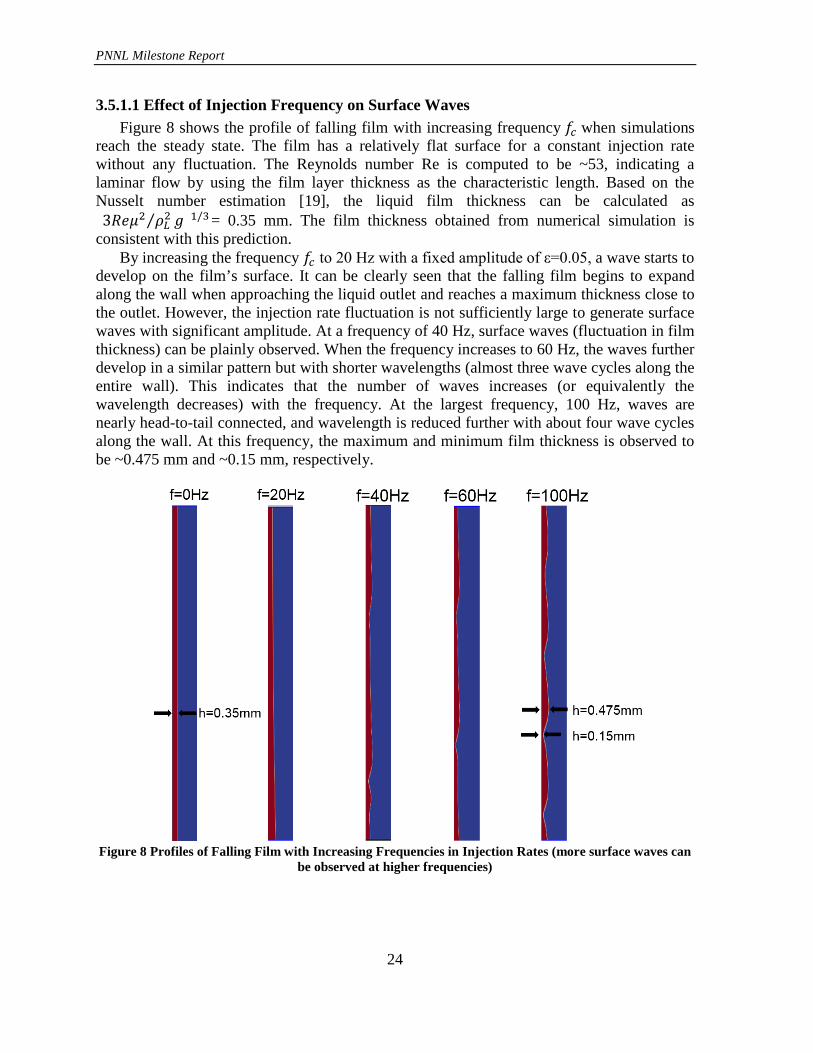
3.5.1.1 Effect of Injection Frequency on Surface Waves Figure 8 shows the profile of falling film with increasing frequency 𝑓𝑓𝑐𝑐 when simulations reach the steady state. The film has a relatively flat surface for a constant injection rate without any fluctuation. The Reynolds number Re is computed to be ~53, indicating a laminar flow by using the film layer thickness as the characteristic length. Based on the Nusselt number estimation [19], the liquid film thickness can be calculated as (3𝑅𝑅𝑒𝑒𝜇𝜇2 𝜌𝜌𝐿𝐿2⁄ 𝑔𝑔)1/3= 0.35 mm. The film thickness obtained from numerical simulation is consistent with this prediction. By increasing the frequency 𝑓𝑓𝑐𝑐 to 20 Hz with a fixed amplitude of ε=0.05, a wave starts to develop on the film’s surface. It can be clearly seen that the falling film begins to expand along the wall when approaching the liquid outlet and reaches a maximum thickness close to the outlet. However, the injection rate fluctuation is not sufficiently large to generate surface waves with significant amplitude. At a frequency of 40 Hz, surface waves (fluctuation in film thickness) can be plainly observed. When the frequency increases to 60 Hz, the waves further develop in a similar pattern but with shorter wavelengths (almost three wave cycles along the entire wall). This indicates that the number of waves increases (or equivalently the wavelength decreases) with the frequency. At the largest frequency, 100 Hz, waves are nearly head-to-tail connected, and wavelength is reduced further with about four wave cycles along the wall. At this frequency, the maximum and minimum film thickness is observed to be ~0.475 mm and ~0.15 mm, respectively.
Figure 8 Profiles of Falling Film with Increasing Frequencies in Injection Rates (more surface waves can
be observed at higher frequencies)

PNNL Milestone Report
25
3.5.1.2 Variation of O2 Concentration for Different Frequencies Figure 9 shows the oxygen concentration distribution along the vertical direction with different injection frequencies. Four cases with different frequencies (𝑓𝑓𝑐𝑐= 20, 40, 60, and 100 Hz) but a fixed amplitude (ε=0.05) are simulated. The horizontal axis in Figure 9 represents the height along the wall (x=0 and 0.0909 m are the gas inlet and outlet locations, respectively), and the vertical axis denotes the concentration of oxygen (in mol/m3) along the vertical line connecting the gas inlet and outlet. The concentration is collected along the central line from gas inlet to outlet. In Figure 9, the outlet concentration will depend on the mass transfer between two phases, i.e., decreasing with increasing mass transfer. The concentration profile in the figure demonstrates that the outlet concentration decreases with increasing frequency 𝑓𝑓𝑐𝑐, indicating an enhanced mass transfer between two phases with increasing frequency, which can correlate to the increasing surface waves shown in Figure 8.
Figure 9 Variation of Gas Concentration Distribution for Different Fluctuation Frequencies (a larger
frequency leads to a steeper concentration gradient in the vertical direction and a larger mass transfer across the interface)
3.5.1.3 Variation of O2 Concentration with Controlled Amplitude Next, the effect of fluctuation amplitude on the mass transfer is investigated by fixing the controlled frequency 𝑓𝑓𝑐𝑐 of the injection rate at 20 Hz but varying the amplitude (ε=0.05, 0.1, 0.15, and 0.2). Figure 10 plots the same concentration profile along the central line from gas

PNNL Milestone Report
26
inlet to outlet. The increase in fluctuation amplitude will result in an immediate decrease in outlet concentration, indicating an enhancement of mass transfer at larger amplitudes. This is expected because surface waves with larger amplitude create large surface area and breathe in more gas along the moving path to enhance the gas absorption [19].
Figure 10 Variation of Gas Concentration Distribution for Different Fluctuation Amplitudes in the
Injection Rate (a larger amplitude leads to a steeper concentration gradient along the vertical direction)
3.5.2 N2O/MEA System A total of 151 numerical simulation cases have been performed for the N2O-MEA non-reactive system.
1) Run No. 1-20. The controlled input parameters are the same as the experimental settings. The calibrated parameters are calculated from the equations introduced in Section 3.2.
2) Run No. 21-43. The controlled input parameters are identical to those of case No. 7 but with different samplings of calibrated parameters, i.e., gas diffusivity in solvent and Henry’s constant.
3) Run No. 43-151. Both controlled and calibrated parameters are systemically tuned to facilitate calibration of the two key parameters.
The model input for controlled and calibrated parameters and numerical results of overall mass transfer coefficient for all 151 cases can be found in the Appendix of this document.

PNNL Milestone Report
27
During the simulation campaigns, the solvent density must be changed to 800 kg/m3 for some cases to avoid crashing the simulations. The run numbers for these cases are: No. 1-6, 10, 11, 13, 16, 44-46, 53-58, 62-64, 80-85, and 89-91. In Section 3.6, we have provided a detailed sensitivity study on solvent density, and the results show this factor has no impact on the mass transfer coefficient, instead merely helping computational convergence. Figure 11 illustrates the comparison between the computed overall mass transfer coefficient and experimental measurement for the first 20 runs, excluding a total of seven unreliable experimental results (No. 1-6, and 10). Section 2 provides detailed information regarding these unreliable data. In addition, there is also one failed simulation case (No. 13) because of numerical instability (800 kg/m3 solvent density will fail the numerical computation and no other solvent density values were evaluated). By excluding those 8 data points, the remaining 12 points shown in Figure 11 scatter around the dash line (slope of 1 indicating a perfect match), indicating that reasonably good agreement between numerical simulation and experimental results has been obtained.
Figure 11 Numerical Simulation Versus Experimental Data for Overall Mass Transfer Coefficient in
N2O/MEA System Figure 12 shows the results of overall mass transfer coefficient versus all six controlled parameters. The orange dots represent numerical results from 12 cases, while the blue dots represent experimental results. It can be observed that mass transfer decreases with MEA mass fraction. On one hand, an increase in MEA mass fraction will increase solvent viscosity, slow down the diffusion process of N2O in MEA, and decelerate the N2O mass transfer. Meanwhile, thickness of the falling solvent film will increase with solvent viscosity for higher MEA mass fraction solvent which leads to a decrease of the average solvent velocity and the advection of falling film if solvent flow rate is kept unchanged. Since N2O concentration in the liquid phase is not uniformly distributed and the region of high N2O concentration locates near the gas-liquid interface, a decrease of advection will reduce the
0.00E+00
5.00E-09
1.00E-08
1.50E-08
2.00E-08
2.50E-08
3.00E-08
3.50E-08
4.00E-08
4.50E-08
0.00E+00 5.00E-09 1.00E-08 1.50E-08 2.00E-08 2.50E-08 3.00E-08 3.50E-08 4.00E-08 4.50E-08
cfd
exp

PNNL Milestone Report
28
mass transfer rate as indicated by eqn. (42). Moreover, the overall mass transfer coefficient also increases with gas flow rate. Theoretically speaking, transport within the liquid phase should control the N2O absorption for a well-mixed gas mixture. In Section 3.6, a parametric study has been performed for small gas flow rate, which proves this factor has only trivial impact on the N2O/MEA mass transfer because the N2O concentration distribution does not have noticeable change for gas flow rates varying from 100 to 300 sccm. There is no obvious tendency observed for the remaining four controlled parameters: temperature, N2O molar fraction, CO2 loading, and solvent flow rate.
0.00E+00
5.00E-09
1.00E-08
1.50E-08
2.00E-08
2.50E-08
3.00E-08
3.50E-08
4.00E-08
0.10 0.20 0.30 0.40
kG
MEAexp cfd
0.00E+00
5.00E-09
1.00E-08
1.50E-08
2.00E-08
2.50E-08
3.00E-08
3.50E-08
4.00E-08
150 200 250 300
kG
Gas flow rate (sccm)
0
5E-09
1E-08
1.5E-08
2E-08
2.5E-08
3E-08
3.5E-08
4E-08
25 35 45 55
kG
Temperature (°C)
0
5E-09
1E-08
1.5E-08
2E-08
2.5E-08
3E-08
3.5E-08
4E-08
0.1 0.2 0.3 0.4 0.5
kG
N2O molar fraction

PNNL Milestone Report
29
Figure 12 kG versus Controlled Parameters in N2O/MEA Systems
Figure 13 shows how mass transfer changes with the two transport parameters, i.e., Henry’s constant and diffusivity. The two dashed lines indicate the replicated experimental results for mass transfer coefficient: 1.95e-8 and 2.02e-8 (mol/Pa·s·m2), respectively. In Figure 13, Henry’s constant has significant impact on the N2O mass transfer. Based on the definition of Henry’s constant (described in Section 3.1), larger Henry’s constant indicates higher solubility of gas in the solvent, which enhances the mass transfer rate into the solvent. Conversely, an increase in gas diffusivity in the solvent only slightly increases the mass transfer coefficient. This is expected because the advection contribution should be much larger compared to that from diffusion on the falling film.
Figure 13 kG versus Henry’s Constant and Diffusivity
0
5E-09
1E-08
1.5E-08
2E-08
2.5E-08
3E-08
3.5E-08
4E-08
0 0.2 0.4 0.6
kG
CO2 Loading
0
5E-09
1E-08
1.5E-08
2E-08
2.5E-08
3E-08
3.5E-08
4E-08
300 400 500 600
kG
Solvent flow rate (ml/min)
1.50E-08
1.70E-08
1.90E-08
2.10E-08
2.30E-08
2.50E-08
2.70E-08
2.90E-08
0.37 0.39 0.41 0.43 0.45 0.47 0.49
kG
Henry's constant
1.50E-08
1.70E-08
1.90E-08
2.10E-08
2.30E-08
2.50E-08
2.70E-08
2.90E-08
9.00E-010 1.10E-009 1.30E-009 1.50E-009 1.70E-009
kG
Diffusivity

PNNL Milestone Report
30
3.5.3 CO2/MEA System The first batch of simulations contains a total of 167 cases. For each experimental run, the corresponding numerical simulations employ the same controlled parameters but with three different values for each calibrated parameter, i.e., Henry’s constant, gas diffusivity in solvent, and CO2 reaction rate constant. The calibrated parameters are systemically adjusted to facilitate the calibration. Five numerical testing cases were conducted for each experimental run (No. 2-29), while a total of 27 numerical testing cases were designed for experimental run No. 1. Detailed model input and numerical results of the overall mass transfer coefficient for all 167 cases can be found in the Appendix within this document. Like the N2O/MEA system, the solvent density must be changed to 800 kg/m3 for the following runs in CO2/MEA system to ensure numerical stability: No. 38-42, 48-57, 63-67, 78-87, 98-102, 108-112, 128-132, and 148-152. In addition, for run No. 43-47, 153-157, and 163-167, the solvent outlet size has to be expanded from 1 mm to 1.5 mm to avoid solvent flooding due to large solvent viscosity. One additional run was carried out to see if a 50% increase in solvent outlet size would significantly affect the mass transfer coefficient. Run No. 1 was selected as the basis, and the solvent outlet size was adjusted from 1 mm to 1.5 mm. Nevertheless, the simulation result differs only by 0.2%, which demonstrates the result is not sensitive to the solvent outlet’s size. Figure 14 compares the predicted mass transfer coefficient and experimental measurement results for the CO2/MEA system. Sets 1 through 5 represent five different numerical designs for each experimental run. In general, the mass transfer coefficients predicted by numerical simulations are in good agreement with the corresponding experimental results. However, numerical simulations predict slightly lower mass transfer coefficients than the experimental measurements, particularly for conditions with relatively large overall mass transfer coefficients. .
Figure 14 Numerical Simulation Versus Experimental Data for Overall Mass Transfer Coefficient in
CO2/MEA Systems
0.00E+00
5.00E-07
1.00E-06
1.50E-06
2.00E-06
2.50E-06
3.00E-06
3.50E-06
0.00E+00 5.00E-07 1.00E-06 1.50E-06 2.00E-06 2.50E-06 3.00E-06 3.50E-06
cfd
exp
set1
set2
set3
set4
set5
PNNL Milestone Report
31
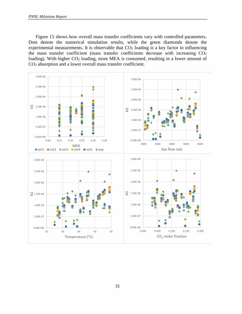
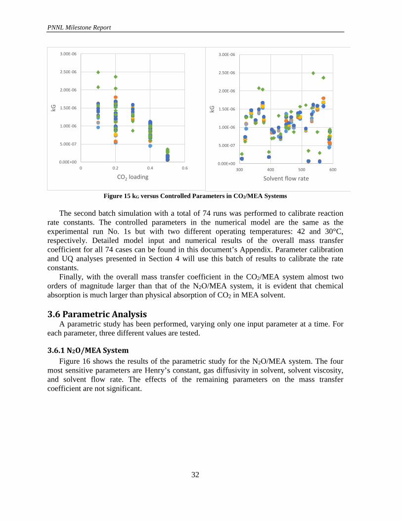
Figure 15 shows how overall mass transfer coefficients vary with controlled parameters. Dots denote the numerical simulation results, while the green diamonds denote the experimental measurements. It is observable that CO2 loading is a key factor in influencing the mass transfer coefficient (mass transfer coefficients decrease with increasing CO2 loading). With higher CO2 loading, more MEA is consumed, resulting in a lower amount of CO2 absorption and a lower overall mass transfer coefficient.
0.00E+00
5.00E-07
1.00E-06
1.50E-06
2.00E-06
2.50E-06
3.00E-06
0.00 0.10 0.20 0.30 0.40 0.50
kG
MEAset1 set2 set3 set4 set5 exp
0.00E+00
5.00E-07
1.00E-06
1.50E-06
2.00E-06
2.50E-06
3.00E-06
2000 3000 4000 5000 6000
kG
Gas flow rate
0.00E+00
5.00E-07
1.00E-06
1.50E-06
2.00E-06
2.50E-06
3.00E-06
20 30 40 50 60
kG
Temperature (°C)
0.00E+00
5.00E-07
1.00E-06
1.50E-06
2.00E-06
2.50E-06
3.00E-06
0.000 0.050 0.100 0.150 0.200
kG
CO2 molar fraction
PNNL Milestone Report
32
Figure 15 kG versus Controlled Parameters in CO2/MEA Systems
The second batch simulation with a total of 74 runs was performed to calibrate reaction rate constants. The controlled parameters in the numerical model are the same as the experimental run No. 1s but with two different operating temperatures: 42 and 30°C, respectively. Detailed model input and numerical results of the overall mass transfer coefficient for all 74 cases can be found in this document’s Appendix. Parameter calibration and UQ analyses presented in Section 4 will use this batch of results to calibrate the rate constants. Finally, with the overall mass transfer coefficient in the CO2/MEA system almost two orders of magnitude larger than that of the N2O/MEA system, it is evident that chemical absorption is much larger than physical absorption of CO2 in MEA solvent. 3.6 Parametric Analysis A parametric study has been performed, varying only one input parameter at a time. For each parameter, three different values are tested.
3.6.1 N2O/MEA System Figure 16 shows the results of the parametric study for the N2O/MEA system. The four most sensitive parameters are Henry’s constant, gas diffusivity in solvent, solvent viscosity, and solvent flow rate. The effects of the remaining parameters on the mass transfer coefficient are not significant.
0.00E+00
5.00E-07
1.00E-06
1.50E-06
2.00E-06
2.50E-06
3.00E-06
0 0.2 0.4 0.6
kG
CO2 loading
0.00E+00
5.00E-07
1.00E-06
1.50E-06
2.00E-06
2.50E-06
3.00E-06
300 400 500 600
kG
Solvent flow rate

PNNL Milestone Report
33
Figure 16 N2O/MEA Parametric Study
A larger Henry’s constant will increase the mass transfer coefficient. Gas diffusivity in solvent will start to affect gas mass transfer once it becomes comparable with the gravity-driven advection from the falling film. Solvent viscosity can differ for different MEA fractions. An increase in solvent viscosity for higher MEA fraction in solvent will reduce advection of the solvent due to the expansion of the falling film thickness. Meanwhile, lower gas diffusivity in solvent and hence significantly decreases the gas-liquid mass transfer. In addition, larger solvent flow rate will help increase the mass transfer by supplying more fresh solvent in unit time. The rest parameters do not have major influence on the predicted mass transfer coefficient.
3.6.2 CO2/MEA System Figure 17 depicts the results of a parametric study for the CO2/MEA system. Because chemical absorption is a major contributor in gas-liquid mass transfer, larger gas diffusivity in both phases will increase the reaction rate by providing more available CO2 near the gas-liquid interface. On the contrary, the Henry’s constant and solvent viscosity become less important because the effect of physical absorption only takes up a small portion of the overall mass transfer coefficient.

PNNL Milestone Report
34
Figure 17 CO2/MEA Parametric Study
3.7 Summary of the Results Fully coupled multiphase flow CFD simulations with hydrodynamics, mass transfer, and chemical reactions have been implemented to compute the mass transfer coefficient in WWC using OpenFOAM, a free and open-source CFD software package with a custom solver. The effects of surface wave frequency and amplitude on the overall mass transfer have been investigated for O2/water systems. Simulation results have been validated via comparison to experimental measurements. A parametric study has been performed to systematically examine the influential factors for WWC performance. Some preliminary findings from the CFD study are summarized as follows:
1) Both wave frequency and amplitude enhance the mass transfer rate for O2/water systems.
2) The mass transfer coefficient decreases with MEA mass fraction for non-reactive N2O/MEA systems.
3) The mass transfer coefficient decreases with CO2 loading for reactive CO2/MEA systems.
4) Chemical absorption is the major contribution to CO2 capture compared to physical absorption.

PNNL Milestone Report
35
5) Henry’s constant, gas diffusivity in solvent, solvent viscosity and solvent flow rate are key parameters determining the physical absorption rate in N2O/MEA systems.
6) Gas diffusivity in both phases plays an important part in the overall mass transfer for the chemical absorption in CO2-MEA system.
4. Model Calibration and UQ Analysis for WWC Experiments Statistical calibration is the process of combining experimental and simulated data to probabilistically infer simulator settings that make its output most consistent with the physical data [21]. A calibration exercise begins by identifying one or more response variables (y) that can be measured in physical experiments and also obtained as output from the corresponding computer model. The identification of experimental and calibration inputs follows. The experimental variables (collected in the vector x) are common to both and are selected because of their potential effect on the response. The calibration inputs t are unique to the computer and inference on their most plausible values θ is desired. After a prior distribution is assigned to θ, a Bayesian Markov chain Monte Carlo algorithm is used to combine that prior with the information given in the simulated and experimental data. Specific and technical details can be found in [21]. The end result of a calibration exercise is a posterior probability distribution on θ and information about a discrepancy function δ(x) that attempts to capture the misfit of the simulated model to the real physical system. For the WWC experiments, the output of interest is the mass transfer coefficient (kG) that relates flux to partial pressure. The following experimental conditions were identified as relevant xs to vary between experiments: operating temperature, MEA mass fraction, CO2 loading in MEA, solvent flow rate, gas flow rate (either N2O or CO2), and inlet gas concentration. Ranges of feasible values also were determined, and these are given in Table 10 and Table 13 for non-reacting (N2O/MEA) and reacting (CO2/MEA) cases, respectively. The simulation model takes these conditions, and calibration inputs, as inputs. For the non-reacting scenario, these inputs are Henry’s coefficient and diffusivity. The reacting scenario has an additional parameter, reaction rate constant. Specifically, Henry’s constant and diffusivity are transport properties that will be calibrated in Unit Problem 2 by a laboratory-scale WWC experiment of the N2O/MEA system. The posterior transport properties will be used as the input a priori in Unit Problem 3, and the rate constant of CO2 will be calibrated in Unit Problem 3 with a laboratory-scale WWC experiment of CO2/MEA systems. All calibration inputs actually are functions of the experimental settings, and these correlations from the literature are given in Table 11 and Table 14. Hence, the goal becomes calibrating the coefficients within the functional relationships and comparing them to their previous estimates expressed in the literature (those estimates also are in the aforementioned tables). This is done for the non-reacting scenario first, then the reacting case. 4.1 N2O/MEA System The statistical design for the experimental data points (i.e., the matrix of how to vary x between different experiments) was chosen to accommodate the fact that few experiments can be conducted with the given budget. First, a 4x5 factorial design was devised using the levels {0.1, 0.2, 0.3, and 0.4} for MEA mass fraction and {0.1, 0.2, 0.3, 0.4, and 0.5} for CO2 loading. From these, 11 points were selected so they were sufficiently “spread out.” These

PNNL Milestone Report
36
values were combined with a space-filling Latin hypercube design in the remaining four variables, subject to their respective ranges. From the resulting design of 11 points in six input variables, one point was chosen to be a replicate. In addition, the central value of the design space (given in Table 10) was used for two more replicate points. Thus, the final experimental design had 14 total points with some carefully chosen replicates.
Table 10 Inputs to the Computer Model for the Non-reacting Case Input Range / Units Experimental, x: Temperature MEA mass fraction CO2 loading in MEA Solvent flow rate Gas flow rate Inlet N2O molar concentration
[25, 60] °C [0.1, 0.4] g MEA/g total [0.0, 0.5] mol CO2/mol MEA [300, 600] ccm [100, 300] sccm [0.15, 0.50] mol/L
Calibration, t: (HN2O) Henry’s coefficient (DN2O) Diffusivity
[0.2, 0.9] unitless; converted from “HN2O,units” [5e-10, 5e-08] m2/s
To determine a simulation design and prior distributions of the calibration parameters, it first was necessary to parameterize Henry’s coefficient and diffusivity (the functional relationships from the literature are given in Table 11). From these correlations, somewhat conservative priors were determined. They are conservative in the sense that they allow for more uncertainty in the true values of Henry’s coefficient and diffusivity than the literature. These priors can be found in Table 12. Two batches of simulations were run resulting in a total sample size of 151. The statistical design for each used heuristic reasoning as well as formal principles: points were selected to be sufficiently “spread out” while still being close to the experimental data in the x-space.
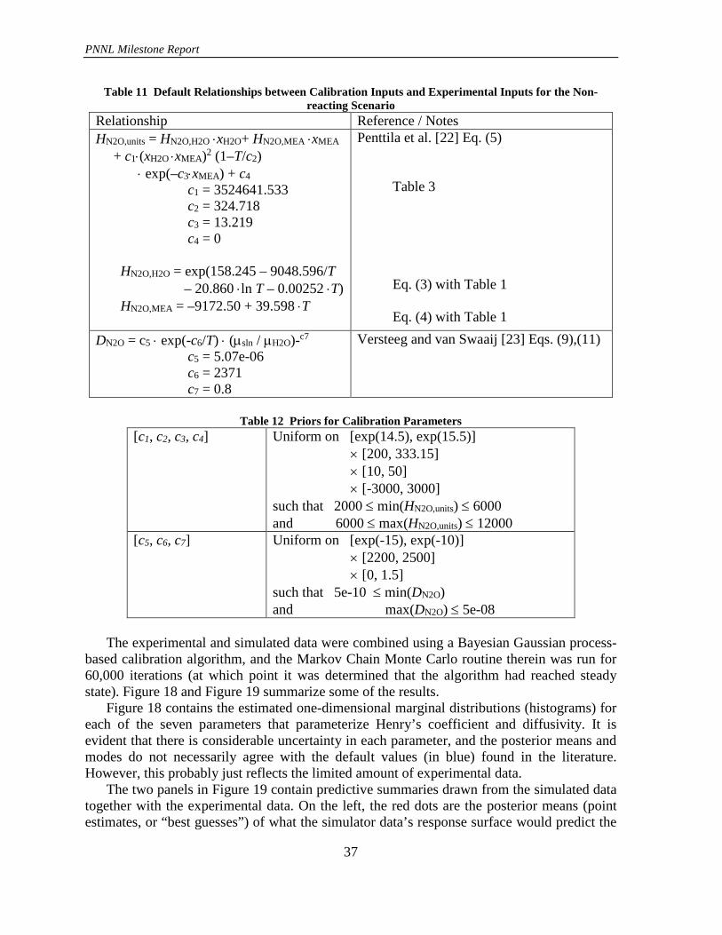
PNNL Milestone Report
37
Table 11 Default Relationships between Calibration Inputs and Experimental Inputs for the Non-reacting Scenario
Relationship Reference / Notes HN2O,units = HN2O,H2O ⋅xH2O+ HN2O,MEA ⋅xMEA + c1⋅(xH2O ⋅xMEA)2 (1–T/c2) ⋅ exp(–c3⋅xMEA) + c4 c1 = 3524641.533 c2 = 324.718 c3 = 13.219 c4 = 0 HN2O,H2O = exp(158.245 – 9048.596/T – 20.860 ⋅ln T – 0.00252 ⋅T) HN2O,MEA = –9172.50 + 39.598 ⋅T
Penttila et al. [22] Eq. (5) Table 3 Eq. (3) with Table 1 Eq. (4) with Table 1
DN2O = c5 ⋅ exp(-c6/T) ⋅ (µsln / µH2O)-c7
c5 = 5.07e-06 c6 = 2371 c7 = 0.8
Versteeg and van Swaaij [23] Eqs. (9),(11)
Table 12 Priors for Calibration Parameters
[c1, c2, c3, c4] Uniform on [exp(14.5), exp(15.5)] × [200, 333.15] × [10, 50] × [-3000, 3000] such that 2000 ≤ min(HN2O,units) ≤ 6000 and 6000 ≤ max(HN2O,units) ≤ 12000
[c5, c6, c7] Uniform on [exp(-15), exp(-10)] × [2200, 2500] × [0, 1.5] such that 5e-10 ≤ min(DN2O) and max(DN2O) ≤ 5e-08
The experimental and simulated data were combined using a Bayesian Gaussian process-based calibration algorithm, and the Markov Chain Monte Carlo routine therein was run for 60,000 iterations (at which point it was determined that the algorithm had reached steady state). Figure 18 and Figure 19 summarize some of the results. Figure 18 contains the estimated one-dimensional marginal distributions (histograms) for each of the seven parameters that parameterize Henry’s coefficient and diffusivity. It is evident that there is considerable uncertainty in each parameter, and the posterior means and modes do not necessarily agree with the default values (in blue) found in the literature. However, this probably just reflects the limited amount of experimental data. The two panels in Figure 19 contain predictive summaries drawn from the simulated data together with the experimental data. On the left, the red dots are the posterior means (point estimates, or “best guesses”) of what the simulator data’s response surface would predict the
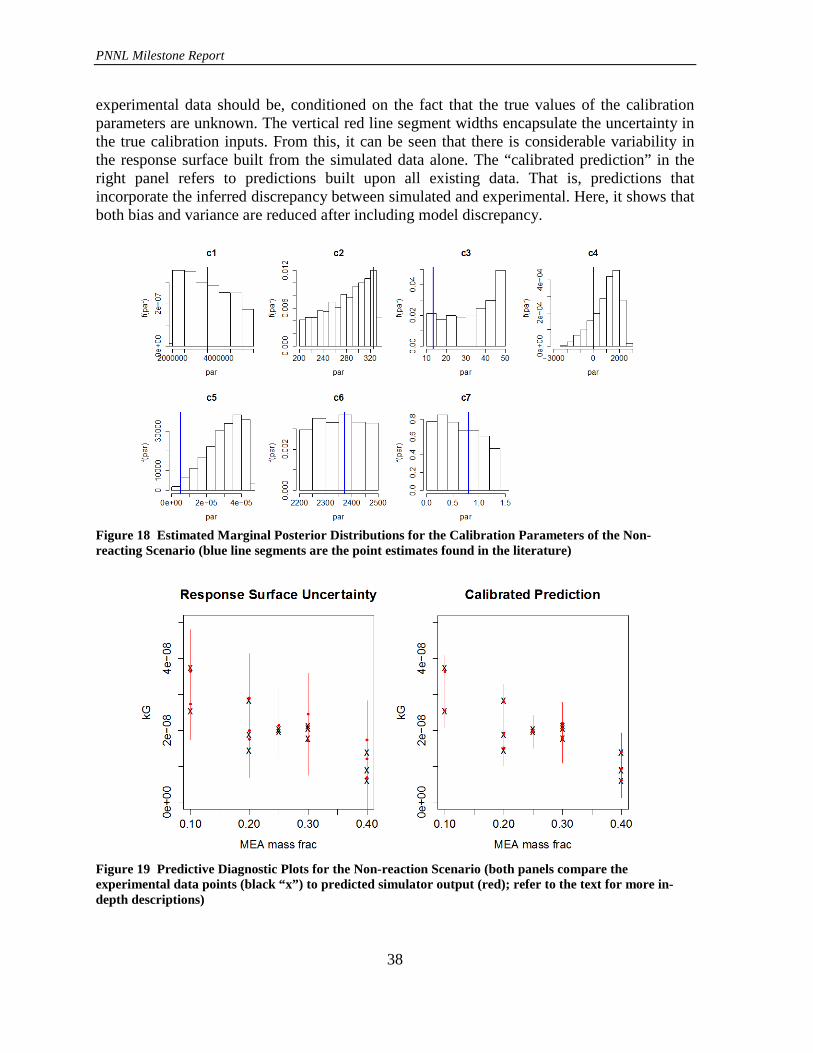
PNNL Milestone Report
38
experimental data should be, conditioned on the fact that the true values of the calibration parameters are unknown. The vertical red line segment widths encapsulate the uncertainty in the true calibration inputs. From this, it can be seen that there is considerable variability in the response surface built from the simulated data alone. The “calibrated prediction” in the right panel refers to predictions built upon all existing data. That is, predictions that incorporate the inferred discrepancy between simulated and experimental. Here, it shows that both bias and variance are reduced after including model discrepancy.
Figure 18 Estimated Marginal Posterior Distributions for the Calibration Parameters of the Non-reacting Scenario (blue line segments are the point estimates found in the literature)
Figure 19 Predictive Diagnostic Plots for the Non-reaction Scenario (both panels compare the experimental data points (black “x”) to predicted simulator output (red); refer to the text for more in-depth descriptions)
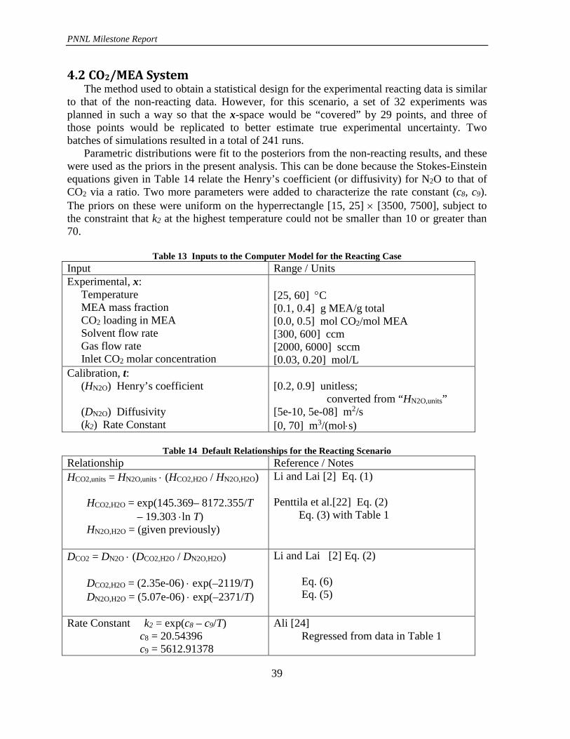
PNNL Milestone Report
39
4.2 CO2/MEA System The method used to obtain a statistical design for the experimental reacting data is similar to that of the non-reacting data. However, for this scenario, a set of 32 experiments was planned in such a way so that the x-space would be “covered” by 29 points, and three of those points would be replicated to better estimate true experimental uncertainty. Two batches of simulations resulted in a total of 241 runs. Parametric distributions were fit to the posteriors from the non-reacting results, and these were used as the priors in the present analysis. This can be done because the Stokes-Einstein equations given in Table 14 relate the Henry’s coefficient (or diffusivity) for N2O to that of CO2 via a ratio. Two more parameters were added to characterize the rate constant (c8, c9). The priors on these were uniform on the hyperrectangle [15, 25] × [3500, 7500], subject to the constraint that k2 at the highest temperature could not be smaller than 10 or greater than 70.
Table 13 Inputs to the Computer Model for the Reacting Case Input Range / Units Experimental, x: Temperature MEA mass fraction CO2 loading in MEA Solvent flow rate Gas flow rate Inlet CO2 molar concentration
[25, 60] °C [0.1, 0.4] g MEA/g total [0.0, 0.5] mol CO2/mol MEA [300, 600] ccm [2000, 6000] sccm [0.03, 0.20] mol/L
Calibration, t: (HN2O) Henry’s coefficient (DN2O) Diffusivity (k2) Rate Constant
[0.2, 0.9] unitless; converted from “HN2O,units” [5e-10, 5e-08] m2/s [0, 70] m3/(mol⋅s)
Table 14 Default Relationships for the Reacting Scenario
Relationship Reference / Notes HCO2,units = HN2O,units ⋅ (HCO2,H2O / HN2O,H2O) HCO2,H2O = exp(145.369– 8172.355/T – 19.303 ⋅ln T) HN2O,H2O = (given previously)
Li and Lai [2] Eq. (1) Penttila et al.[22] Eq. (2) Eq. (3) with Table 1
DCO2 = DN2O ⋅ (DCO2,H2O / DN2O,H2O) DCO2,H2O = (2.35e-06) ⋅ exp(–2119/T) DN2O,H2O = (5.07e-06) ⋅ exp(–2371/T)
Li and Lai [2] Eq. (2) Eq. (6) Eq. (5)
Rate Constant k2 = exp(c8 – c9/T) c8 = 20.54396 c9 = 5612.91378
Ali [24] Regressed from data in Table 1

PNNL Milestone Report
40
To achieve convergence, the calibration routine was run for a total of 110,000 iterations, and Figure 20 and Figure 21 show the results. It can be seen that the posteriors for c1–c7 (parameterizing Henry’s coefficient and diffusivity) after this calibration are not qualitatively different from the posteriors following the non-reacting calibration. That is, there was not much information about these quantities after combining the experimental and simulated reacting data. The data seemingly only informs the parameterization of the rate constant, but this could be reasonable.
Figure 20 Estimated Marginal Posterior Distributions for the Calibration Parameters of the Reacting Scenario (blue line segments are the point estimates found in the literature)

PNNL Milestone Report
41
Figure 21 Uncertainty, the Rate Constant, as a Function of Temperature (C) (blue curve is derived from the literature, while the black curve is the median prediction; the dashed lines form pointwise 90% intervals)
Figure 22 Predictive Diagnostic Plots for the Reacting Scenario (both panels compare the experimental data points (black “x”) to predicted simulator output (red); refer to the text for more in-depth descriptions)
The panels of Figure 22 tell a similar story: before incorporating the experimental observations, the response surface based upon the simulations has a fair amount of variation that can potentially mimic the trend of the experimental data (left). However, after learning the model discrepancy, the calibrated predictions are centered on the correct values and have uncertainties related purely to small experimental error (right). By the end of this second analysis, we have demonstrated that the Bayesian calibration methodology can be used to validate models, as well as quantify and propagate parametric
PNNL Milestone Report
42
uncertainties. From here, it would be possible, for example, to pass the samples from the second stage posteriors through a model of an upscaled system to get prediction intervals.
Acknowledgments Pacific Northwest National Laboratory is operated by Battelle for the U.S. Department of Energy (DOE) under Contract No. DE-AC05-76RL01830. This work was funded by the DOE Office of Fossil Energy’s Carbon Capture Simulation Initiative through the National Energy Technology Laboratory.
References 1. Sun, X., et al., A Validation Hierarchy for CFD Models of Solvent-based Carbon
Capture Systems. 2015, PNNL: Richland, WA 2. Li, M.H. and M.D. Lai, Solubility and Diffusivity of N2o and Co2 in
(Monoethanolamine Plus N-Methyldiethanolamine Plus Water) and in (Monoethanolamine Plus 2-Amino-2-Methyl-1-Propanol Plus Water). Journal of Chemical and Engineering Data, 1995. 40(2): p. 486-492.
3. Weiland, R.H., et al., Density and viscosity of some partially carbonated aqueous alkanolamine solutions and their blends. Journal of Chemical and Engineering Data, 1998. 43(3): p. 378-382.
4. Astronautics, A.I.o.A.A., AIAA Guide for the Verification and Validation of Computational Fluid Dynamics Simulations. AIAA G-077-1998. 1998, Renton, VA: American Institute of Aeronautics & Astronautics.
5. Oberkampf, W.L. and C.J. Roy, Verification and Validation in Scientific Computing. 2010: Cambridge University Press.
6. Aronu, U.E., et al., Solubility of CO2 in 15, 30, 45 and 60 mass% MEA from 40 to 120 degrees C and model representation using the extended UNIQUAC framework. Chemical Engineering Science, 2011. 66(24): p. 6393-6406.
7. Brackbill, J.U., D.B. Kothe, and C. Zemach, A Continuum Method for Modeling Surface-Tension. Journal of Computational Physics, 1992. 100(2): p. 335-354.
8. Haroun, Y., D. Legendre, and L. Raynal, Direct numerical simulation of reactive absorption in gas-liquid flow on structured packing using interface capturing method. Chemical Engineering Science, 2010. 65(1): p. 351-356.
9. Astarita, G., D.W. Savage, and A. Bistro, Gas Treating with Chemical Solvents. 1983, New York: John Wiley & Sons.
10. Danckwerts, P.V., Gas–Liquid Reactions. 1970: McGraw-Hill Book Company. 11. Gabrielsen, J., et al., A model for estimating CO2 solubility in aqueous
alkanolamines. Industrial & Engineering Chemistry Research, 2005. 44(9): p. 3348-3354.
12. Hikita, H., et al., Kinetics of Reactions of Carbon-Dioxide with Monoethanolamine, Diethanolamine and Triethanolamine by a Rapid Mixing Method. Chemical Engineering Journal and the Biochemical Engineering Journal, 1977. 13(1): p. 7-12.
13. Khan, F.M. and T. Mahmud Modelling of Gas Absorbers for Carbon Dioxide Capture Applications.

PNNL Milestone Report
43
14. Snijder, E.D., et al., Diffusion-Coefficients of Several Aqueous Alkanolamine Solutions. Journal of Chemical and Engineering Data, 1993. 38(3): p. 475-480.
15. Wilke, C.R., A Viscosity Equation for Gas Mixtures. Journal of Chemical Physics, 1950. 18(4): p. 517-519.
16. Cussler, E.L., Diffusion: Mass Transfer in Fluid Systems. 2nd ed. 1997: New York: Cambridge University Press.
17. Fu, D., et al., Experiments and model for the surface tension of carbonated monoethanolamine aqueous solutions. Science China-Chemistry, 2012. 55(7): p. 1467-1473.
18. Gao, D., N.B. Morley, and V. Dhir, Numerical simulation of wavy falling film flow using VOF method. Journal of Computational Physics, 2003. 192(2): p. 624-642.
19. Hu, J.G., et al., Numerical simulation of carbon dioxide (CO2) absorption and interfacial mass transfer across vertically wavy falling film. Chemical Engineering Science, 2014. 116: p. 243-253.
20. Xu, Z.F., B.C. Khoo, and N.E. Wijeysundera, Mass transfer across the falling film: Simulations and experiments. Chemical Engineering Science, 2008. 63(9): p. 2559-2575.
21. Kennedy, M.C. and A. O'Hagan, Bayesian calibration of computer models. Journal of the Royal Statistical Society Series B-Statistical Methodology, 2001. 63: p. 425-450.
22. Penttila, A., et al., The Henry's law constant of N2O and CO2 in aqueous binary and ternary amine solutions (MEA, DEA, DIPA, MDEA, and AMP). Fluid Phase Equilibria, 2011. 311: p. 59-66.
23. Versteeg, G.F. and W.P.M. Vanswaaij, Solubility and Diffusivity of Acid Gases (Co2, N2o) in Aqueous Alkanolamine Solutions. Journal of Chemical and Engineering Data, 1988. 33(1): p. 29-34.
24. Ali, S.H., Kinetics of the reaction of carbon dioxide with blends of amines in aqueous media using the stopped-flow technique. International Journal of Chemical Kinetics, 2005. 37(7): p. 391-405.
Appendix N2O/MEA
ID MEA CO2 Loading Temperature
Solvent Flow Rate
Gas Flow Rate
N2O Conc.
Henry’s Constant Diffusivity kG
1 0.2992 0.464 35 350 200 0.15 0.474659 7.86E-010 2.75E-08
2 0.2992 0.464 45 350 200 0.15 0.412627 1.04E-009 1.83E-08
3 0.2992 0.464 55 350 200 0.15 0.364716 1.35E-009 1.55E-08
4 0.2992 0.5 35 350 200 0.15 0.474659 7.66E-010 2.56E-08
5 0.2992 0.5 45 350 200 0.15 0.412627 1.01E-009 1.74E-08
6 0.2992 0.5 55 350 200 0.15 0.364716 1.31E-009 1.53E-08
7 0.25 0.3 42 450 200 0.325 0.426731 1.30E-009 2.37E-08
8 0.1 0.1 40 509.48 211.01 0.228 0.440978 2.08E-009 3.11E-08
9 0.1 0.3 37 585.92 268.38 0.43 0.466508 1.87E-009 3.60E-08
10 0.1 0.5 31 381.4 137.97 0.351 0.526328 1.55E-009 3.34E-08
11 0.2 0.1 28 308.78 299.62 0.483 0.536734 1.14E-009 2.65E-08
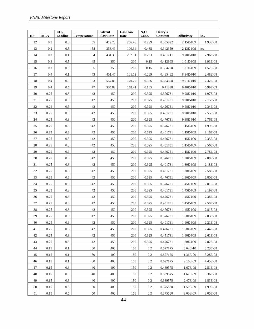
PNNL Milestone Report
44
ID MEA CO2 Loading Temperature
Solvent Flow Rate
Gas Flow Rate
N2O Conc.
Henry’s Constant Diffusivity kG
12 0.2 0.3 55 412.78 256.46 0.299 0.355022 2.15E-009 1.93E-08
13 0.2 0.5 58 358.49 100.34 0.435 0.342359 2.13E-009 n/a
14 0.3 0.1 34 431.39 232.31 0.203 0.481741 9.78E-010 2.96E-08
15 0.3 0.5 45 350 200 0.15 0.412695 1.01E-009 1.93E-08
16 0.3 0.5 55 350 200 0.15 0.364798 1.31E-009 1.52E-08
17 0.4 0.1 43 451.47 181.52 0.289 0.435482 8.94E-010 2.48E-08
18 0.4 0.3 53 557.88 170.25 0.386 0.384308 9.51E-010 2.32E-08
19 0.4 0.5 47 535.83 158.41 0.165 0.41338 6.40E-010 6.99E-09
20 0.25 0.3 42 450 200 0.325 0.376731 9.98E-010 1.97E-08
21 0.25 0.3 42 450 200 0.325 0.401731 9.98E-010 2.15E-08
22 0.25 0.3 42 450 200 0.325 0.426731 9.98E-010 2.34E-08
23 0.25 0.3 42 450 200 0.325 0.451731 9.98E-010 2.55E-08
24 0.25 0.3 42 450 200 0.325 0.476731 9.98E-010 2.76E-08
25 0.25 0.3 42 450 200 0.325 0.376731 1.15E-009 1.99E-08
26 0.25 0.3 42 450 200 0.325 0.401731 1.15E-009 2.16E-08
27 0.25 0.3 42 450 200 0.325 0.426731 1.15E-009 2.35E-08
28 0.25 0.3 42 450 200 0.325 0.451731 1.15E-009 2.56E-08
29 0.25 0.3 42 450 200 0.325 0.476731 1.15E-009 2.78E-08
30 0.25 0.3 42 450 200 0.325 0.376731 1.30E-009 2.00E-08
31 0.25 0.3 42 450 200 0.325 0.401731 1.30E-009 2.18E-08
32 0.25 0.3 42 450 200 0.325 0.451731 1.30E-009 2.58E-08
33 0.25 0.3 42 450 200 0.325 0.476731 1.30E-009 2.80E-08
34 0.25 0.3 42 450 200 0.325 0.376731 1.45E-009 2.01E-08
35 0.25 0.3 42 450 200 0.325 0.401731 1.45E-009 2.19E-08
36 0.25 0.3 42 450 200 0.325 0.426731 1.45E-009 2.38E-08
37 0.25 0.3 42 450 200 0.325 0.451731 1.45E-009 2.59E-08
38 0.25 0.3 42 450 200 0.325 0.476731 1.45E-009 2.81E-08
39 0.25 0.3 42 450 200 0.325 0.376731 1.60E-009 2.03E-08
40 0.25 0.3 42 450 200 0.325 0.401731 1.60E-009 2.21E-08
41 0.25 0.3 42 450 200 0.325 0.426731 1.60E-009 2.44E-08
42 0.25 0.3 42 450 200 0.325 0.451731 1.60E-009 2.61E-08
43 0.25 0.3 42 450 200 0.325 0.476731 1.60E-009 2.82E-08
44 0.15 0.1 30 400 150 0.2 0.527175 8.64E-10 3.23E-08
45 0.15 0.1 30 400 150 0.2 0.527175 1.36E-09 3.28E-08
46 0.15 0.1 30 400 150 0.2 0.627175 2.16E-09 4.45E-08
47 0.15 0.3 40 400 150 0.2 0.439575 1.67E-09 2.51E-08
48 0.15 0.3 40 400 150 0.2 0.539575 1.67E-09 3.36E-08
49 0.15 0.3 40 400 150 0.2 0.339575 2.47E-09 1.83E-08
50 0.15 0.5 50 400 150 0.2 0.375588 1.50E-09 1.99E-08
51 0.15 0.5 50 400 150 0.2 0.375588 2.00E-09 2.05E-08

PNNL Milestone Report
45
ID MEA CO2 Loading Temperature
Solvent Flow Rate
Gas Flow Rate
N2O Conc.
Henry’s Constant Diffusivity kG
52 0.15 0.5 50 400 150 0.2 0.275588 2.80E-09 1.45E-08
53 0.25 0.1 40 400 150 0.2 0.439309 1.36E-09 2.42E-08
54 0.25 0.1 40 400 150 0.2 0.539309 1.36E-09 3.27E-08
55 0.25 0.1 40 400 150 0.2 0.439309 2.16E-09 2.47E-08
56 0.25 0.3 50 400 150 0.2 0.382694 1.06E-09 1.92E-08
57 0.25 0.3 50 400 150 0.2 0.382694 1.56E-09 1.94E-08
58 0.25 0.3 50 400 150 0.2 0.482694 1.56E-09 2.73E-08
59 0.25 0.5 30 400 150 0.2 0.512564 3.04E-10 3.07E-08
60 0.25 0.5 30 400 150 0.2 0.512564 8.04E-10 3.22E-08
61 0.25 0.5 30 400 150 0.2 0.612564 1.60E-09 4.31E-08
62 0.35 0.1 50 400 150 0.2 0.492264 8.45E-10 2.78E-08
63 0.35 0.1 50 400 150 0.2 0.292264 1.35E-09 1.35E-08
64 0.35 0.1 50 400 150 0.2 0.392264 1.35E-09 2.02E-08
65 0.35 0.3 30 400 150 0.2 0.515216 1.20E-10 3.44E-08
66 0.35 0.3 30 400 150 0.2 0.515216 6.20E-10 3.46E-08
67 0.35 0.3 30 400 150 0.2 0.415216 1.42E-09 2.83E-08
68 0.35 0.5 40 400 150 0.2 0.546548 1.89E-10 3.98E-08
69 0.35 0.5 40 400 150 0.2 0.346548 6.89E-10 2.19E-08
70 0.35 0.5 40 400 150 0.2 0.446548 6.89E-10 3.01E-08
71 0.15 0.1 30 400 250 0.2 0.627175 8.64E-10 4.36E-08
72 0.15 0.1 30 400 250 0.2 0.527175 1.36E-09 3.35E-08
73 0.15 0.1 30 400 250 0.2 0.627175 2.16E-09 4.53E-08
74 0.15 0.3 40 400 250 0.2 0.439575 1.17E-09 2.45E-08
75 0.15 0.3 40 400 250 0.2 0.439575 1.67E-09 2.51E-08
76 0.15 0.3 40 400 250 0.2 0.539575 2.47E-09 3.53E-08
77 0.15 0.5 50 400 250 0.2 0.475588 1.50E-09 2.73E-08
78 0.15 0.5 50 400 250 0.2 0.275588 2.00E-09 1.37E-08
79 0.15 0.5 50 400 250 0.2 0.375588 2.00E-09 2.05E-08
80 0.25 0.1 40 400 250 0.2 0.339309 8.57E-10 1.64E-08
81 0.25 0.1 40 400 250 0.2 0.339309 1.36E-09 1.67E-08
82 0.25 0.1 40 400 250 0.2 0.439309 1.36E-09 2.42E-08
83 0.25 0.3 50 400 250 0.2 0.282694 1.56E-09 1.32E-08
84 0.25 0.3 50 400 250 0.2 0.382694 1.56E-09 2.00E-08
85 0.25 0.3 50 400 250 0.2 0.482694 2.36E-09 2.85E-08
86 0.25 0.5 30 400 250 0.2 0.612564 3.04E-10 4.38E-08
87 0.25 0.5 30 400 250 0.2 0.512564 8.04E-10 3.57E-08
88 0.25 0.5 30 400 250 0.2 0.412564 1.60E-09 2.85E-08
89 0.35 0.1 50 400 250 0.2 0.392264 1.35E-09 2.02E-08
90 0.35 0.1 50 400 250 0.2 0.292264 2.15E-09 1.38E-08
91 0.35 0.1 50 400 250 0.2 0.492264 2.15E-09 2.86E-08

PNNL Milestone Report
46
ID MEA CO2 Loading Temperature
Solvent Flow Rate
Gas Flow Rate
N2O Conc.
Henry’s Constant Diffusivity kG
92 0.35 0.3 30 400 250 0.2 0.415216 1.20E-10 2.35E-08
93 0.35 0.3 30 400 250 0.2 0.515216 6.20E-10 3.12E-08
94 0.35 0.3 30 400 250 0.2 0.415216 1.42E-09 2.46E-08
95 0.35 0.5 40 400 250 0.2 0.446548 1.89E-10 2.90E-08
96 0.35 0.5 40 400 250 0.2 0.346548 6.89E-10 2.19E-08
97 0.35 0.5 40 400 250 0.2 0.446548 6.89E-10 2.93E-08
98 0.15 0.1 30 500 150 0.4 0.427175 8.64E-10 2.56E-08
99 0.15 0.1 30 500 150 0.4 0.527175 8.64E-10 3.36E-08
100 0.15 0.1 30 500 150 0.4 0.527175 1.36E-09 3.49E-08
101 0.15 0.3 40 500 150 0.4 0.539575 1.17E-09 3.48E-08
102 0.15 0.3 40 500 150 0.4 0.439575 1.67E-09 2.83E-08
103 0.15 0.3 40 500 150 0.4 0.539575 1.67E-09 3.65E-08
104 0.15 0.5 50 500 150 0.4 0.275588 1.50E-09 1.62E-08
105 0.15 0.5 50 500 150 0.4 0.475588 1.50E-09 3.03E-08
106 0.15 0.5 50 500 150 0.4 0.375588 2.00E-09 2.45E-08
107 0.25 0.1 40 500 150 0.4 0.439309 8.57E-10 2.44E-08
108 0.25 0.1 40 500 150 0.4 0.439309 1.36E-09 2.52E-08
109 0.25 0.1 40 500 150 0.4 0.539309 1.36E-09 3.43E-08
110 0.25 0.3 50 500 150 0.4 0.482694 1.06E-09 2.80E-08
111 0.25 0.3 50 500 150 0.4 0.282694 1.56E-09 1.48E-08
112 0.25 0.3 50 500 150 0.4 0.382694 1.56E-09 2.12E-08
113 0.25 0.5 30 500 150 0.4 0.512564 8.04E-10 3.76E-08
114 0.25 0.5 30 500 150 0.4 0.612564 8.04E-10 4.95E-08
115 0.25 0.5 30 500 150 0.4 0.512564 1.60E-09 3.93E-08
116 0.35 0.1 50 500 150 0.4 0.492264 8.45E-10 2.71E-08
117 0.35 0.1 50 500 150 0.4 0.292264 1.35E-09 1.46E-08
118 0.35 0.1 50 500 150 0.4 0.392264 1.35E-09 2.05E-08
119 0.35 0.3 30 500 150 0.4 0.415216 1.20E-10 3.04E-08
120 0.35 0.3 30 500 150 0.4 0.515216 6.20E-10 4.08E-08
121 0.35 0.3 30 500 150 0.4 0.415216 1.42E-09 3.07E-08
122 0.35 0.5 40 500 150 0.4 0.446548 6.89E-10 3.89E-08
123 0.35 0.5 40 500 150 0.4 0.546548 6.89E-10 5.00E-08
124 0.35 0.5 40 500 150 0.4 0.446548 1.49E-09 4.41E-08
125 0.15 0.1 30 500 250 0.4 0.527175 1.36E-09 3.51E-08
126 0.15 0.1 30 500 250 0.4 0.427175 2.16E-09 2.77E-08
127 0.15 0.1 30 500 250 0.4 0.527175 2.16E-09 3.73E-08
128 0.15 0.3 40 500 250 0.4 0.339575 1.17E-09 2.02E-08
129 0.15 0.3 40 500 250 0.4 0.439575 1.67E-09 2.83E-08
130 0.15 0.3 40 500 250 0.4 0.539575 2.47E-09 3.91E-08
131 0.15 0.5 50 500 250 0.4 0.375588 1.50E-09 2.32E-08
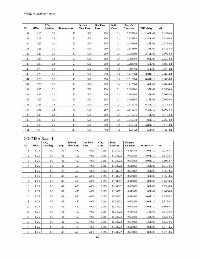
PNNL Milestone Report
47
ID MEA CO2 Loading Temperature
Solvent Flow Rate
Gas Flow Rate
N2O Conc.
Henry’s Constant Diffusivity kG
132 0.15 0.5 50 500 250 0.4 0.375588 2.00E-09 2.45E-08
133 0.15 0.5 50 500 250 0.4 0.375588 2.80E-09 2.64E-08
134 0.25 0.1 40 500 250 0.4 0.439309 1.36E-09 2.53E-08
135 0.25 0.1 40 500 250 0.4 0.539309 1.36E-09 3.42E-08
136 0.25 0.1 40 500 250 0.4 0.539309 2.16E-09 3.60E-08
137 0.25 0.3 50 500 250 0.4 0.382694 1.06E-09 2.02E-08
138 0.25 0.3 50 500 250 0.4 0.282694 1.56E-09 1.48E-08
139 0.25 0.3 50 500 250 0.4 0.382694 1.56E-09 2.12E-08
140 0.25 0.5 30 500 250 0.4 0.412564 3.04E-10 2.78E-08
141 0.25 0.5 30 500 250 0.4 0.512564 8.04E-10 3.98E-08
142 0.25 0.5 30 500 250 0.4 0.412564 1.60E-09 2.78E-08
143 0.35 0.1 50 500 250 0.4 0.392264 1.35E-09 2.05E-08
144 0.35 0.1 50 500 250 0.4 0.392264 2.15E-09 2.20E-08
145 0.35 0.1 50 500 250 0.4 0.492264 2.15E-09 2.96E-08
146 0.35 0.3 30 500 250 0.4 0.515216 6.20E-10 4.24E-08
147 0.35 0.3 30 500 250 0.4 0.615216 6.20E-10 5.00E-08
148 0.35 0.3 30 500 250 0.4 0.515216 1.42E-09 4.37E-08
149 0.35 0.5 40 500 250 0.4 0.346548 1.89E-10 2.66E-08
150 0.35 0.5 40 500 250 0.4 0.446548 6.89E-10 3.47E-08
151 0.35 0.5 40 500 250 0.4 0.446548 1.49E-09 3.56E-08
CO2/MEA Batch 1
ID MEA CO2 Loading Temp
Solvent Flow Rate
Gas Flow Rate
CO2 Conc.
Rate Constant
Henry’s Constant Diffusivity kG
1 0.25 0.3 42 450 4000 0.115 11.38922 0.511896 8.04E-10 9.03E-07
2 0.25 0.3 42 450 4000 0.115 11.38922 0.601896 8.04E-10 9.14E-07
3 0.25 0.3 42 450 4000 0.115 11.38922 0.671896 8.04E-10 9.19E-07
4 0.25 0.3 42 450 4000 0.115 11.38922 0.511896 1.30E-09 1.04E-06
5 0.25 0.3 42 450 4000 0.115 11.38922 0.601896 1.30E-09 1.05E-06
6 0.25 0.3 42 450 4000 0.115 11.38922 0.671896 1.30E-09 1.05E-06
7 0.25 0.3 42 450 4000 0.115 11.38922 0.511896 1.80E-09 1.14E-06
8 0.25 0.3 42 450 4000 0.115 11.38922 0.601896 1.80E-09 1.15E-06
9 0.25 0.3 42 450 4000 0.115 11.38922 0.671896 1.80E-09 1.16E-06
10 0.25 0.3 42 450 4000 0.115 15.38922 0.511896 8.04E-10 9.75E-07
11 0.25 0.3 42 450 4000 0.115 15.38922 0.601896 8.04E-10 9.81E-07
12 0.25 0.3 42 450 4000 0.115 15.38922 0.671896 8.04E-10 9.86E-07
13 0.25 0.3 42 450 4000 0.115 15.38922 0.511896 1.30E-09 1.11E-06
14 0.25 0.3 42 450 4000 0.115 15.38922 0.601896 1.30E-09 1.12E-06
15 0.25 0.3 42 450 4000 0.115 15.38922 0.671896 1.30E-09 1.13E-06
16 0.25 0.3 42 450 4000 0.115 15.38922 0.511896 1.80E-09 1.21E-06
17 0.25 0.3 42 450 4000 0.115 15.38922 0.601896 1.80E-09 1.22E-06

PNNL Milestone Report
48
ID MEA CO2 Loading Temp
Solvent Flow Rate
Gas Flow Rate
CO2 Conc.
Rate Constant
Henry’s Constant Diffusivity kG
18 0.25 0.3 42 450 4000 0.115 15.38922 0.671896 1.80E-09 1.23E-06
19 0.25 0.3 42 450 4000 0.115 19.38922 0.511896 8.04E-10 1.03E-06
20 0.25 0.3 42 450 4000 0.115 19.38922 0.601896 8.04E-10 1.04E-06
21 0.25 0.3 42 450 4000 0.115 19.38922 0.671896 8.04E-10 1.04E-06
22 0.25 0.3 42 450 4000 0.115 19.38922 0.511896 1.30E-09 1.17E-06
23 0.25 0.3 42 450 4000 0.115 19.38922 0.601896 1.30E-09 1.18E-06
24 0.25 0.3 42 450 4000 0.115 19.38922 0.671896 1.30E-09 1.18E-06
25 0.25 0.3 42 450 4000 0.115 19.38922 0.511896 1.80E-09 1.27E-06
26 0.25 0.3 42 450 4000 0.115 19.38922 0.601896 1.80E-09 1.28E-06
27 0.25 0.3 42 450 4000 0.115 19.38922 0.671896 1.80E-09 1.29E-06
28 0.1 0.1 45 494.75 4343.63 0.07 14.20342 0.631912 2.36E-09 1.23E-06
29 0.1 0.1 45 494.75 4343.63 0.07 14.20342 0.631912 2.76E-09 1.28E-06
30 0.1 0.1 45 494.75 4343.63 0.07 18.20342 0.571912 2.36E-09 1.29E-06
31 0.1 0.1 45 494.75 4343.63 0.07 22.20342 0.571912 1.96E-09 1.29E-06
32 0.1 0.1 45 494.75 4343.63 0.07 22.20342 0.631912 2.76E-09 1.41E-06
33 0.1 0.2 27 590.24 2126.49 0.191 2.319231 0.709204 1.52E-09 5.36E-07
34 0.1 0.2 27 590.24 2126.49 0.191 2.319231 0.709204 1.92E-09 5.72E-07
35 0.1 0.2 27 590.24 2126.49 0.191 6.319231 0.789204 1.52E-09 7.32E-07
36 0.1 0.2 27 590.24 2126.49 0.191 10.31923 0.789204 1.12E-09 7.68E-07
37 0.1 0.2 27 590.24 2126.49 0.191 10.31923 0.789204 1.92E-09 8.89E-07
38 0.1 0.2 49 351.91 2724.41 0.086 18.66149 0.458428 2.92E-09 1.15E-06
39 0.1 0.2 49 351.91 2724.41 0.086 22.66149 0.598428 2.12E-09 1.12E-06
40 0.1 0.2 49 351.91 2724.41 0.086 22.66149 0.538428 2.52E-09 1.16E-06
41 0.1 0.2 49 351.91 2724.41 0.086 26.66149 0.458428 2.52E-09 1.19E-06
42 0.1 0.2 49 351.91 2724.41 0.086 26.66149 0.598428 2.52E-09 1.20E-06
43 0.1 0.3 55 550.02 2557.81 0.164 27.16327 0.49553 2.79E-09 1.49E-06
44 0.1 0.3 55 550.02 2557.81 0.164 31.16327 0.49553 2.39E-09 1.48E-06
45 0.1 0.3 55 550.02 2557.81 0.164 31.16327 0.49553 2.79E-09 1.52E-06
46 0.1 0.3 55 550.02 2557.81 0.164 35.16327 0.41553 2.79E-09 1.54E-06
47 0.1 0.3 55 550.02 2557.81 0.164 35.16327 0.55553 3.19E-09 1.59E-06
48 0.1 0.4 47 318.21 2284.11 0.183 16.32441 0.554637 2.71E-09 6.95E-07
49 0.1 0.4 47 318.21 2284.11 0.183 20.32441 0.474637 1.91E-09 6.69E-07
50 0.1 0.4 47 318.21 2284.11 0.183 20.32441 0.554637 2.31E-09 7.07E-07
51 0.1 0.4 47 318.21 2284.11 0.183 24.32441 0.474637 1.91E-09 6.98E-07
52 0.1 0.4 47 318.21 2284.11 0.183 24.32441 0.554637 2.31E-09 7.36E-07
53 0.1 0.4 59 404.19 3474.06 0.158 34.29151 0.531131 2.96E-09 8.73E-07
54 0.1 0.4 59 404.19 3474.06 0.158 38.29151 0.391131 2.56E-09 8.54E-07
55 0.1 0.4 59 404.19 3474.06 0.158 38.29151 0.471131 2.96E-09 8.89E-07
56 0.1 0.4 59 404.19 3474.06 0.158 42.29151 0.471131 3.36E-09 9.34E-07
57 0.1 0.4 59 404.19 3474.06 0.158 42.29151 0.531131 3.36E-09 9.39E-07
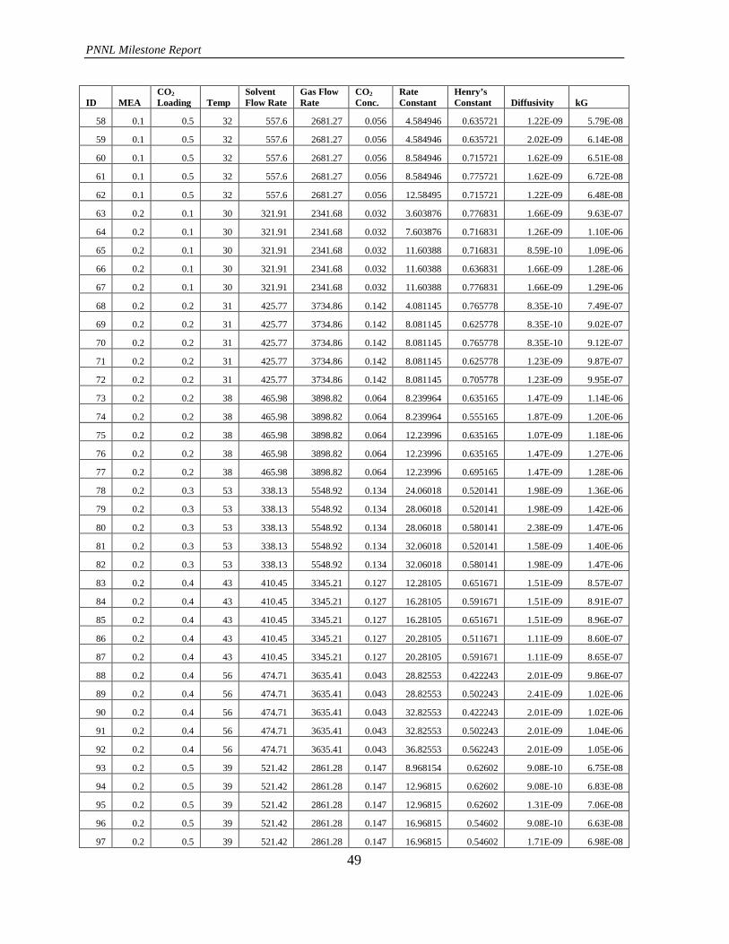
PNNL Milestone Report
49
ID MEA CO2 Loading Temp
Solvent Flow Rate
Gas Flow Rate
CO2 Conc.
Rate Constant
Henry’s Constant Diffusivity kG
58 0.1 0.5 32 557.6 2681.27 0.056 4.584946 0.635721 1.22E-09 5.79E-08
59 0.1 0.5 32 557.6 2681.27 0.056 4.584946 0.635721 2.02E-09 6.14E-08
60 0.1 0.5 32 557.6 2681.27 0.056 8.584946 0.715721 1.62E-09 6.51E-08
61 0.1 0.5 32 557.6 2681.27 0.056 8.584946 0.775721 1.62E-09 6.72E-08
62 0.1 0.5 32 557.6 2681.27 0.056 12.58495 0.715721 1.22E-09 6.48E-08
63 0.2 0.1 30 321.91 2341.68 0.032 3.603876 0.776831 1.66E-09 9.63E-07
64 0.2 0.1 30 321.91 2341.68 0.032 7.603876 0.716831 1.26E-09 1.10E-06
65 0.2 0.1 30 321.91 2341.68 0.032 11.60388 0.716831 8.59E-10 1.09E-06
66 0.2 0.1 30 321.91 2341.68 0.032 11.60388 0.636831 1.66E-09 1.28E-06
67 0.2 0.1 30 321.91 2341.68 0.032 11.60388 0.776831 1.66E-09 1.29E-06
68 0.2 0.2 31 425.77 3734.86 0.142 4.081145 0.765778 8.35E-10 7.49E-07
69 0.2 0.2 31 425.77 3734.86 0.142 8.081145 0.625778 8.35E-10 9.02E-07
70 0.2 0.2 31 425.77 3734.86 0.142 8.081145 0.765778 8.35E-10 9.12E-07
71 0.2 0.2 31 425.77 3734.86 0.142 8.081145 0.625778 1.23E-09 9.87E-07
72 0.2 0.2 31 425.77 3734.86 0.142 8.081145 0.705778 1.23E-09 9.95E-07
73 0.2 0.2 38 465.98 3898.82 0.064 8.239964 0.635165 1.47E-09 1.14E-06
74 0.2 0.2 38 465.98 3898.82 0.064 8.239964 0.555165 1.87E-09 1.20E-06
75 0.2 0.2 38 465.98 3898.82 0.064 12.23996 0.635165 1.07E-09 1.18E-06
76 0.2 0.2 38 465.98 3898.82 0.064 12.23996 0.635165 1.47E-09 1.27E-06
77 0.2 0.2 38 465.98 3898.82 0.064 12.23996 0.695165 1.47E-09 1.28E-06
78 0.2 0.3 53 338.13 5548.92 0.134 24.06018 0.520141 1.98E-09 1.36E-06
79 0.2 0.3 53 338.13 5548.92 0.134 28.06018 0.520141 1.98E-09 1.42E-06
80 0.2 0.3 53 338.13 5548.92 0.134 28.06018 0.580141 2.38E-09 1.47E-06
81 0.2 0.3 53 338.13 5548.92 0.134 32.06018 0.520141 1.58E-09 1.40E-06
82 0.2 0.3 53 338.13 5548.92 0.134 32.06018 0.580141 1.98E-09 1.47E-06
83 0.2 0.4 43 410.45 3345.21 0.127 12.28105 0.651671 1.51E-09 8.57E-07
84 0.2 0.4 43 410.45 3345.21 0.127 16.28105 0.591671 1.51E-09 8.91E-07
85 0.2 0.4 43 410.45 3345.21 0.127 16.28105 0.651671 1.51E-09 8.96E-07
86 0.2 0.4 43 410.45 3345.21 0.127 20.28105 0.511671 1.11E-09 8.60E-07
87 0.2 0.4 43 410.45 3345.21 0.127 20.28105 0.591671 1.11E-09 8.65E-07
88 0.2 0.4 56 474.71 3635.41 0.043 28.82553 0.422243 2.01E-09 9.86E-07
89 0.2 0.4 56 474.71 3635.41 0.043 28.82553 0.502243 2.41E-09 1.02E-06
90 0.2 0.4 56 474.71 3635.41 0.043 32.82553 0.422243 2.01E-09 1.02E-06
91 0.2 0.4 56 474.71 3635.41 0.043 32.82553 0.502243 2.01E-09 1.04E-06
92 0.2 0.4 56 474.71 3635.41 0.043 36.82553 0.562243 2.01E-09 1.05E-06
93 0.2 0.5 39 521.42 2861.28 0.147 8.968154 0.62602 9.08E-10 6.75E-08
94 0.2 0.5 39 521.42 2861.28 0.147 12.96815 0.62602 9.08E-10 6.83E-08
95 0.2 0.5 39 521.42 2861.28 0.147 12.96815 0.62602 1.31E-09 7.06E-08
96 0.2 0.5 39 521.42 2861.28 0.147 16.96815 0.54602 9.08E-10 6.63E-08
97 0.2 0.5 39 521.42 2861.28 0.147 16.96815 0.54602 1.71E-09 6.98E-08
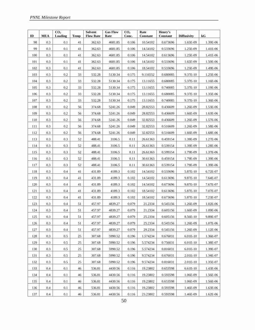
PNNL Milestone Report
50
ID MEA CO2 Loading Temp
Solvent Flow Rate
Gas Flow Rate
CO2 Conc.
Rate Constant
Henry’s Constant Diffusivity kG
98 0.3 0.1 41 362.63 4681.85 0.106 10.54102 0.673696 1.65E-09 1.39E-06
99 0.3 0.1 41 362.63 4681.85 0.106 14.54102 0.533696 1.25E-09 1.41E-06
100 0.3 0.1 41 362.63 4681.85 0.106 14.54102 0.613696 1.25E-09 1.41E-06
101 0.3 0.1 41 362.63 4681.85 0.106 14.54102 0.533696 1.65E-09 1.50E-06
102 0.3 0.1 41 362.63 4681.85 0.106 18.54102 0.533696 1.25E-09 1.49E-06
103 0.3 0.2 33 532.28 5130.34 0.175 9.116552 0.680085 9.37E-10 1.25E-06
104 0.3 0.2 33 532.28 5130.34 0.175 13.11655 0.680085 5.37E-10 1.16E-06
105 0.3 0.2 33 532.28 5130.34 0.175 13.11655 0.740085 5.37E-10 1.19E-06
106 0.3 0.2 33 532.28 5130.34 0.175 13.11655 0.680085 9.37E-10 1.35E-06
107 0.3 0.2 33 532.28 5130.34 0.175 13.11655 0.740085 9.37E-10 1.36E-06
108 0.3 0.2 56 374.68 5241.26 0.049 28.82553 0.436609 1.26E-09 1.53E-06
109 0.3 0.2 56 374.68 5241.26 0.049 28.82553 0.436609 1.66E-09 1.63E-06
110 0.3 0.2 56 374.68 5241.26 0.049 32.82553 0.436609 1.26E-09 1.57E-06
111 0.3 0.2 56 374.68 5241.26 0.049 32.82553 0.516609 1.26E-09 1.58E-06
112 0.3 0.2 56 374.68 5241.26 0.049 32.82553 0.516609 1.66E-09 1.68E-06
113 0.3 0.3 52 488.41 3106.5 0.11 26.61363 0.459154 1.39E-09 1.27E-06
114 0.3 0.3 52 488.41 3106.5 0.11 26.61363 0.539154 1.39E-09 1.28E-06
115 0.3 0.3 52 488.41 3106.5 0.11 26.61363 0.599154 1.79E-09 1.37E-06
116 0.3 0.3 52 488.41 3106.5 0.11 30.61363 0.459154 1.79E-09 1.39E-06
117 0.3 0.3 52 488.41 3106.5 0.11 30.61363 0.539154 1.79E-09 1.39E-06
118 0.3 0.4 41 431.89 4189.3 0.102 14.54102 0.533696 5.87E-10 6.72E-07
119 0.3 0.4 41 431.89 4189.3 0.102 14.54102 0.613696 9.87E-10 7.64E-07
120 0.3 0.4 41 431.89 4189.3 0.102 14.54102 0.673696 9.87E-10 7.67E-07
121 0.3 0.4 41 431.89 4189.3 0.102 18.54102 0.613696 5.87E-10 7.07E-07
122 0.3 0.4 41 431.89 4189.3 0.102 18.54102 0.673696 5.87E-10 7.23E-07
123 0.3 0.4 51 457.97 4839.27 0.079 21.2334 0.545156 1.26E-09 1.02E-06
124 0.3 0.4 51 457.97 4839.27 0.079 21.2334 0.605156 1.66E-09 1.09E-06
125 0.3 0.4 51 457.97 4839.27 0.079 25.2334 0.605156 8.56E-10 9.89E-07
126 0.3 0.4 51 457.97 4839.27 0.079 25.2334 0.545156 1.26E-09 1.07E-06
127 0.3 0.4 51 457.97 4839.27 0.079 29.2334 0.545156 1.26E-09 1.12E-06
128 0.3 0.5 25 307.68 5990.52 0.196 1.574234 0.676031 6.01E-10 1.36E-07
129 0.3 0.5 25 307.68 5990.52 0.196 5.574234 0.756031 6.01E-10 1.38E-07
130 0.3 0.5 25 307.68 5990.52 0.196 5.574234 0.816031 6.01E-10 1.39E-07
131 0.3 0.5 25 307.68 5990.52 0.196 9.574234 0.676031 2.01E-10 1.34E-07
132 0.3 0.5 25 307.68 5990.52 0.196 9.574234 0.816031 2.01E-10 1.35E-07
133 0.4 0.1 46 536.81 4430.56 0.116 19.23802 0.653598 6.61E-10 1.43E-06
134 0.4 0.1 46 536.81 4430.56 0.116 19.23802 0.593598 1.06E-09 1.56E-06
135 0.4 0.1 46 536.81 4430.56 0.116 19.23802 0.653598 1.06E-09 1.56E-06
136 0.4 0.1 46 536.81 4430.56 0.116 19.23802 0.593598 1.46E-09 1.63E-06
137 0.4 0.1 46 536.81 4430.56 0.116 23.23802 0.593598 1.46E-09 1.62E-06

PNNL Milestone Report
51
ID MEA CO2 Loading Temp
Solvent Flow Rate
Gas Flow Rate
CO2 Conc.
Rate Constant
Henry’s Constant Diffusivity kG
138 0.4 0.2 36 513.12 4065.71 0.121 6.891733 0.590771 1.12E-09 9.05E-07
139 0.4 0.2 36 513.12 4065.71 0.121 6.891733 0.670771 1.12E-09 9.26E-07
140 0.4 0.2 36 513.12 4065.71 0.121 10.89173 0.670771 7.18E-10 9.11E-07
141 0.4 0.2 36 513.12 4065.71 0.121 14.89173 0.670771 7.18E-10 9.34E-07
142 0.4 0.2 36 513.12 4065.71 0.121 14.89173 0.730771 1.12E-09 9.66E-07
143 0.4 0.2 59 569.82 5672.76 0.179 34.29151 0.436382 1.31E-09 1.67E-06
144 0.4 0.2 59 569.82 5672.76 0.179 34.29151 0.576382 1.71E-09 1.80E-06
145 0.4 0.2 59 569.82 5672.76 0.179 38.29151 0.516382 1.31E-09 1.69E-06
146 0.4 0.2 59 569.82 5672.76 0.179 38.29151 0.576382 1.31E-09 1.69E-06
147 0.4 0.2 59 569.82 5672.76 0.179 42.29151 0.516382 9.12E-10 1.58E-06
148 0.4 0.3 34 378.28 5300.57 0.04 5.677291 0.608123 1.00E-09 1.17E-06
149 0.4 0.3 34 378.28 5300.57 0.04 9.677291 0.688123 6.05E-10 1.18E-06
150 0.4 0.3 34 378.28 5300.57 0.04 9.677291 0.608123 1.00E-09 1.24E-06
151 0.4 0.3 34 378.28 5300.57 0.04 9.677291 0.748123 1.00E-09 1.24E-06
152 0.4 0.3 34 378.28 5300.57 0.04 13.67729 0.748123 1.00E-09 1.29E-06
153 0.4 0.4 28 588.01 5790.45 0.093 2.724073 0.743758 4.54E-10 4.49E-07
154 0.4 0.4 28 588.01 5790.45 0.093 6.724073 0.743758 4.54E-10 5.90E-07
155 0.4 0.4 28 588.01 5790.45 0.093 10.72407 0.663758 4.54E-10 6.70E-07
156 0.4 0.4 28 588.01 5790.45 0.093 10.72407 0.743758 4.54E-10 6.73E-07
157 0.4 0.4 28 588.01 5790.45 0.093 10.72407 0.803758 4.54E-10 6.76E-07
158 0.4 0.4 49 449.33 4869.33 0.153 18.66149 0.633549 4.06E-10 9.96E-07
159 0.4 0.4 49 449.33 4869.33 0.153 18.66149 0.633549 8.06E-10 1.04E-06
160 0.4 0.4 49 449.33 4869.33 0.153 22.66149 0.633549 4.06E-10 1.01E-06
161 0.4 0.4 49 449.33 4869.33 0.153 22.66149 0.573549 8.06E-10 1.05E-06
162 0.4 0.4 49 449.33 4869.33 0.153 22.66149 0.633549 1.21E-09 1.08E-06
163 0.4 0.5 37 394.64 3189.22 0.078 7.548359 0.582332 5.23E-10 1.84E-07
164 0.4 0.5 37 394.64 3189.22 0.078 7.548359 0.662332 9.23E-10 1.85E-07
165 0.4 0.5 37 394.64 3189.22 0.078 11.54836 0.662332 5.23E-10 1.85E-07
166 0.4 0.5 37 394.64 3189.22 0.078 11.54836 0.722332 5.23E-10 1.85E-07
167 0.4 0.5 37 394.64 3189.22 0.078 15.54836 0.722332 1.23E-10 1.84E-07
CO2/MEA Batch 2
ID MEA CO2 Loading Temp
Solvent Flow Rate
Gas Flow Rate
CO2 Conc.
Rate Constant
Henry’s Constant Diffusivity kG
1 0.25 0.3 42 450 4000 0.115 26.8653 0.508248 9.49E-09 1.91E-06
2 0.25 0.3 42 450 4000 0.115 25.13401 0.508248 9.49E-09 1.90E-06
3 0.25 0.3 42 450 4000 0.115 11.3627 0.508248 9.49E-09 1.67E-06
4 0.25 0.3 42 450 4000 0.115 23.5143 0.508248 9.49E-09 1.88E-06
5 0.25 0.3 42 450 4000 0.115 11.83765 0.508248 9.49E-09 1.68E-06
6 0.25 0.3 42 450 4000 0.115 24.49717 0.508248 9.49E-09 1.89E-06
7 0.25 0.3 42 450 4000 0.115 22.91849 0.508248 9.49E-09 1.87E-06

PNNL Milestone Report
52
ID MEA CO2 Loading Temp
Solvent Flow Rate
Gas Flow Rate
CO2 Conc.
Rate Constant
Henry’s Constant Diffusivity kG
8 0.25 0.3 42 450 4000 0.115 9.945389 0.508248 9.49E-09 1.63E-06
9 0.25 0.3 42 450 4000 0.115 4.315762 0.508248 9.49E-09 1.33E-06
10 0.25 0.3 42 450 4000 0.115 23.87646 0.508248 9.49E-09 1.88E-06
11 0.25 0.3 42 450 4000 0.115 4.03764 0.508248 9.49E-09 1.31E-06
12 0.25 0.3 42 450 4000 0.115 8.35561 0.508248 9.49E-09 1.57E-06
13 0.25 0.3 42 450 4000 0.115 22.33779 0.508248 9.49E-09 1.87E-06
14 0.25 0.3 42 450 4000 0.115 4.206409 0.508248 9.49E-09 1.33E-06
15 0.25 0.3 42 450 4000 0.115 8.704866 0.508248 9.49E-09 1.58E-06
16 0.25 0.3 42 450 4000 0.115 12.52239 0.508248 9.49E-09 1.70E-06
17 0.25 0.3 42 450 4000 0.115 23.27148 0.508248 9.49E-09 1.88E-06
18 0.25 0.3 42 450 4000 0.115 3.935335 0.508248 9.49E-09 1.30E-06
19 0.25 0.3 42 450 4000 0.115 10.52068 0.508248 9.49E-09 1.64E-06
20 0.25 0.3 42 450 4000 0.115 21.7718 0.508248 9.49E-09 1.86E-06
21 0.25 0.3 42 450 4000 0.115 4.099828 0.508248 9.49E-09 1.32E-06
22 0.25 0.3 42 450 4000 0.115 20.36875 0.508248 9.49E-09 1.84E-06
23 0.25 0.3 42 450 4000 0.115 8.838938 0.508248 9.49E-09 1.59E-06
24 0.25 0.3 42 450 4000 0.115 3.835622 0.508248 9.49E-09 1.29E-06
25 0.25 0.3 42 450 4000 0.115 11.41857 0.508248 9.49E-09 1.67E-06
26 0.25 0.3 42 450 4000 0.115 21.22014 0.508248 9.49E-09 1.85E-06
27 0.25 0.3 42 450 4000 0.115 3.995947 0.508248 9.49E-09 1.31E-06
28 0.25 0.3 42 450 4000 0.115 19.85265 0.508248 9.49E-09 1.83E-06
29 0.25 0.3 42 450 4000 0.115 3.738435 0.508248 9.49E-09 1.28E-06
30 0.25 0.3 42 450 4000 0.115 7.736427 0.508248 9.49E-09 1.54E-06
31 0.25 0.3 42 450 4000 0.115 8.059802 0.508248 9.49E-09 1.56E-06
32 0.25 0.3 42 450 4000 0.115 3.497519 0.508248 9.49E-09 1.26E-06
33 0.25 0.3 42 450 4000 0.115 8.396693 0.508248 9.49E-09 1.57E-06
34 0.25 0.3 42 450 4000 0.115 3.643711 0.508248 9.49E-09 1.27E-06
35 0.25 0.3 42 450 4000 0.115 3.408899 0.508248 9.49E-09 1.25E-06
36 0.25 0.3 42 450 4000 0.115 3.954685 0.508248 9.49E-09 1.30E-06
37 0.25 0.3 42 450 4000 0.115 15.13453 0.508248 9.49E-09 1.76E-06
38 0.25 0.3 30 450 4000 0.115 15.00799 0.598017 7.12E-09 1.66E-06
39 0.25 0.3 30 450 4000 0.115 13.80372 0.598017 7.12E-09 1.64E-06
40 0.25 0.3 30 450 4000 0.115 6.135064 0.598017 7.12E-09 1.39E-06
41 0.25 0.3 30 450 4000 0.115 12.69608 0.598017 7.12E-09 1.61E-06
42 0.25 0.3 30 450 4000 0.115 6.310382 0.598017 7.12E-09 1.40E-06
43 0.25 0.3 30 450 4000 0.115 13.05889 0.598017 7.12E-09 1.62E-06
44 0.25 0.3 30 450 4000 0.115 12.01102 0.598017 7.12E-09 1.60E-06
45 0.25 0.3 30 450 4000 0.115 5.189988 0.598017 7.12E-09 1.33E-06
46 0.25 0.3 30 450 4000 0.115 2.242606 0.598017 7.12E-09 1.07E-06
47 0.25 0.3 30 450 4000 0.115 12.35425 0.598017 7.12E-09 1.60E-06
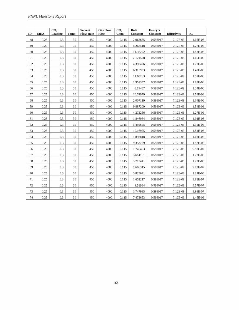
PNNL Milestone Report
53
ID MEA CO2 Loading Temp
Solvent Flow Rate
Gas Flow Rate
CO2 Conc.
Rate Constant
Henry’s Constant Diffusivity kG
48 0.25 0.3 30 450 4000 0.115 2.062655 0.598017 7.12E-09 1.05E-06
49 0.25 0.3 30 450 4000 0.115 4.268518 0.598017 7.12E-09 1.27E-06
50 0.25 0.3 30 450 4000 0.115 11.36292 0.598017 7.12E-09 1.58E-06
51 0.25 0.3 30 450 4000 0.115 2.121598 0.598017 7.12E-09 1.06E-06
52 0.25 0.3 30 450 4000 0.115 4.390496 0.598017 7.12E-09 1.28E-06
53 0.25 0.3 30 450 4000 0.115 6.315953 0.598017 7.12E-09 1.40E-06
54 0.25 0.3 30 450 4000 0.115 11.68763 0.598017 7.12E-09 1.59E-06
55 0.25 0.3 30 450 4000 0.115 1.951357 0.598017 7.12E-09 1.03E-06
56 0.25 0.3 30 450 4000 0.115 5.19457 0.598017 7.12E-09 1.34E-06
57 0.25 0.3 30 450 4000 0.115 10.74979 0.598017 7.12E-09 1.56E-06
58 0.25 0.3 30 450 4000 0.115 2.007119 0.598017 7.12E-09 1.04E-06
59 0.25 0.3 30 450 4000 0.115 9.887209 0.598017 7.12E-09 1.54E-06
60 0.25 0.3 30 450 4000 0.115 4.272286 0.598017 7.12E-09 1.27E-06
61 0.25 0.3 30 450 4000 0.115 1.846064 0.598017 7.12E-09 1.01E-06
62 0.25 0.3 30 450 4000 0.115 5.495695 0.598017 7.12E-09 1.35E-06
63 0.25 0.3 30 450 4000 0.115 10.16975 0.598017 7.12E-09 1.54E-06
64 0.25 0.3 30 450 4000 0.115 1.898818 0.598017 7.12E-09 1.02E-06
65 0.25 0.3 30 450 4000 0.115 9.353709 0.598017 7.12E-09 1.52E-06
66 0.25 0.3 30 450 4000 0.115 1.746453 0.598017 7.12E-09 9.98E-07
67 0.25 0.3 30 450 4000 0.115 3.614161 0.598017 7.12E-09 1.22E-06
68 0.25 0.3 30 450 4000 0.115 3.717441 0.598017 7.12E-09 1.23E-06
69 0.25 0.3 30 450 4000 0.115 1.606315 0.598017 7.12E-09 9.73E-07
70 0.25 0.3 30 450 4000 0.115 3.823671 0.598017 7.12E-09 1.24E-06
71 0.25 0.3 30 450 4000 0.115 1.652217 0.598017 7.12E-09 9.82E-07
72 0.25 0.3 30 450 4000 0.115 1.51964 0.598017 7.12E-09 9.57E-07
73 0.25 0.3 30 450 4000 0.115 1.747995 0.598017 7.12E-09 9.98E-07
74 0.25 0.3 30 450 4000 0.115 7.472653 0.598017 7.12E-09 1.45E-06