pmsm sensorless vector control on kinetis€¢ application speed ranges from 0% to 100% of nominal...

June, 2013 of 55

PMSM Sensorless Vector Control on Kinetis Designer Reference Manual Document Number: DRM140 Rev 1.1, 06/2013 by: Matus Plachy System Application Engineer Freescale

To provide the most up-to-date information, the revision of our documents on the World Wide Web will be the most current. Your printed copy may be an earlier revision. To verify you have the latest information available, refer to:

http://www.freescale.com The following revision history table summarizes changes contained in this document. For your convenience, the page number designators have been linked to the appropriate location.

http://www.freescale.com/�

June, 2013 of 55

Revision History

Date Revision Level

Description Page Number(s)

4-Jan-13 1.0 First Draft N/A 6/7/2013 1.1 Renamed all instances of “Motor Control Tuning

Wizard” to “Motor Control Application Tuning Tool” Renamed all instances of “MCTW” to “MCAT”

N/A

June, 2013 of 55

Table of Contents

SECTION 1. INTRODUCTION .............................................................. 7 Application features ....................................................................................................................... 7 Benefits of our solution ................................................................................................................. 7 References ...................................................................................................................................... 7 Acronyms and Abbreviations ....................................................................................................... 8

SECTION 2. SYSTEM SPECIFICATION .............................................. 9

SECTION 3. SYSTEM DESIGN .......................................................... 10 3.1 Control Theory ................................................................................................................. 10 3.1.1 3-Phase Permanent Magnet Synchronous Motor .......................................................... 10 3.1.2 Introduction to Vector Control ........................................................................................ 10 3.1.3 Sensorless Vector Control Implementation.................................................................... 12 3.1.3.1 Open Loop Start-up and Merging ............................................................................... 14 3.2 Hardware .......................................................................................................................... 15 3.2.1 Hardware Set-up and Configuration .............................................................................. 16

SECTION 4. SOFTWARE DESIGN ..................................................... 19 4.1 Fractional Numbers Representation ............................................................................. 19 4.2 Application Overview ...................................................................................................... 19 4.3 Kinetis K60 Peripheral Modules Configuration ............................................................ 19 4.3.1 FlexTimer0 Configuration for Generating a 6-channel PWM ......................................... 20 4.3.2 ADC and PDB Modules Configuration ........................................................................... 22 4.3.3 ADC Conversion Timing, Currents and Voltage Sampling ............................................ 22 4.3.4 Current Measurement .................................................................................................... 23 4.3.5 SPI Configuration ........................................................................................................... 25 4.3.6 SCI (UART) Configuration.............................................................................................. 25 4.4 Enabling the Interrupts on the Core Level .................................................................... 25 4.5 FreeMASTER Software ................................................................................................... 27 4.5.1 Introduction .................................................................................................................... 27 4.5.2 FreeMASTER Communication Driver ............................................................................ 27 4.5.3 FreeMASTER Recorder and Scope ............................................................................... 27 4.6 Program Flow .................................................................................................................. 28 4.6.1 Application Structure ...................................................................................................... 28 4.6.2 Application Background Loop ........................................................................................ 28 4.6.3 Application State Machine ............................................................................................. 29 4.6.3.1 States Definition .......................................................................................................... 29 4.6.3.2 Motor State Machine ................................................................................................... 32 4.6.4 Sensorless PMS Motor Control ...................................................................................... 36 4.6.4.1 Field Oriented Control ................................................................................................. 36 4.6.4.2 Position and speed estimation .................................................................................... 38 4.6.4.3 Rotor alignment ........................................................................................................... 39 4.6.4.4 Motor open-loop start-up ............................................................................................ 39 4.6.4.5 Slow (speed) control loop ........................................................................................... 41 4.6.5 Scalar Control ................................................................................................................ 42 4.6.6 Control mode selector .................................................................................................... 43 4.7 Interface function ............................................................................................................ 45 4.7.1 Switch control functions ................................................................................................. 45 4.7.2 Command functions ....................................................................................................... 45 4.8 Application parameters .................................................................................................. 46 4.9 Application parameters modification ............................................................................ 47 4.10 Interrupts ........................................................................................................................ 48

June, 2013 of 55

4.10.1 ADC1 Interrupt ............................................................................................................... 49 4.10.2 PORTC interrupt ............................................................................................................ 50 4.10.3 PDB Error interrupt ......................................................................................................... 51

SECTION 5. APPLICATION SET-UP AND OPERATION ................... 53

SECTION 6. RESULTS OF THE MEASUREMENT ............................ 53 6.1 CPU Load and the Execution Time ................................................................................ 53 6.2 Measured Results Using FreeMASTER ......................................................................... 54 6.2.1 Motor Start-up ................................................................................................................ 54 6.2.2 Position Merging ............................................................................................................ 54

June, 2013 of 55

List of Figures and Tables

Figure Title Page FIGURE 3-1 SYNCHRONOUS MACHINE AND THE MAIN PRINCIPLE OF THE VECTOR CONTROL ............................................. 11FIGURE 3-2 TRANSFORMATION SEQUENCING .................................................................................................................. 12FIGURE 3-3 BLOCK DIAGRAM OF SENSORLESS PMSM VECTOR CONTROL ....................................................................... 14FIGURE 3-4 HARDWARE BUILT ON THE MODULES OF THE TOWER SYSTEM ....................................................................... 16FIGURE 3-5 JUMPERS AND CONNECTORS POSITIONS ON THE TWR-MC-LV3PH .............................................................. 17FIGURE 4-1 ADC CONVERSION TIMING ........................................................................................................................... 23FIGURE 4-2 CURRENT SENSING ..................................................................................................................................... 24FIGURE 4-3 APPLICATION STRUCTURE ............................................................................................................................ 28FIGURE 4-4 APPLICATION STATE MACHINE DIAGRAM ....................................................................................................... 29FIGURE 4-5 MOTOR RUN SUB-STATE DIAGRAM ................................................................................................................ 34FIGURE 4-6 START-UP PROCESS ................................................................................................................................... 41FIGURE 4-7 BLOCK DIAGRAM OF THE SCALAR CONTROL ................................................................................................... 43FIGURE 4-8 ADC ISR FLOW CHART ................................................................................................................................ 50FIGURE 6-1 MOTOR STARTUP FROM ZERO SPEED TO 2000 RPM ....................................................................................... 54

June, 2013 of 55

Table Title Page TABLE 1-1 ACRONYMS AND ABBREVIATED TERMS ............................................................................................................. 8TABLE 3-1 JUMPER SETTINGS OF TWR-MC-LV3PH BOARD ........................................................................................... 17TABLE 3-2 MOTOR AND ENCODER CONNECTORS ON THE TWR-MC-LV3PH .................................................................... 17TABLE 3-3 SPECIFICATION OF THE MOTOR ...................................................................................................................... 18TABLE 4-1 KINETIS K60 PERIPHERALS OVERVIEW ........................................................................................................... 19TABLE 4-2 MEMORY USAGE, VALUES IN BYTES ............................................................................................................... 53

June, 2013 of 55

Section 1. Introduction This paper describes the design of a sensorless vector control drive of the 3-phase permanent magnet synchronous motor (PMSM). The application runs on the Kinetis K60 ARM® Cortex™-M4 microcontroller. The document is more focused on the application implementation on the Kinetis K60 microcontroller, and only briefly describes the theory of the PMSM vector control, as it is well described in the referenced literature. Although the paper describes implementation on the Kinetis K60, the application can successfully run on any of the microcontrollers from the Kinetis family.

Application features

• Sensorless vector control of a permanent magnet synchronous motor • Back-EMF observer used as a sensorless position estimator algorithm • Open loop start-up until 10% of nominal speed • Targeted at the Tower rapid prototyping system (K60 tower board, Tower 3-phase low

voltage power stage) • Vector control with a speed closed-loop • Rotation in both directions • Application speed ranges from 0% to 100% of nominal speed (no field weakening) • Operation via user’s buttons on the Kinetis K60 tower board or via FreeMASTER software

Benefits of our solution

Kinetis is a mixed-signal MCU family based on the new ARM Cortex-M4 core and the most scalable portfolio of mixed-signal ARM Cortex-M4 MCUs in the industry. Five performance options are available from 50 to 150 MHz, with flash memory ranging from 32 KB to 1 MB, and high RAM-to-flash ratios throughout. Common peripherals, memory maps and packages both within and across the MCU families allow for easy migration to greater/less memory and functionality. A vector control algorithm, demonstrated in this application, enables vector control of the PMSM with no need of position feedback sensor (encoder or resolver), while keeping high dynamic performance above 10% of nominal speed.

References

[1] K60P144M150SF3RM - K60 Sub-Family Reference Manual, Freescale Semiconductor, 2011 [2] DRM110 - Sensorless PMSM Control for an H-axis Washing Machine Drive, Designer

Reference Manual, Freescale Semiconductor, 2010 [3] DRM105 - PM Sinusoidal Motor Vector Control with Quadrature Encoder, Designer

Reference Manual, Freescale Semiconductor, 2008 [4] Set of General Math and Motor Control Functions for Cortex M4 Core, User Reference

Manual, Freescale Semiconductor, 2011 [5] ACLCM4UG - Advanced Control Library for Cortex-M4 Core, User Reference Manual,

Freescale Semiconductor, 2012 [6] AN3729 - Using FlexTimer in ACIM/PMSM Motor Control Applications, Freescale

Semiconductor, 2008

June, 2013 of 55

[7] MC33937, Three Phase Field Effect Transistor Pre-driver, Freescale Semiconductor 2009 [8] ARM®v7-M Architecture Reference Manual, ARM Limited 2010 [9] K60P144M100SF2V2 – K60 Sub-Family Data Sheet, Freescale Semiconductor 2012 [10] AN1948 - Real Time Development of MC Applications using the PC Master Software

Visualization Tool , Freescale Semiconductor 2005 [11] TWR‐MC‐LV3PH User’s Manual, Freescale Semiconductor 2011 [12] PMSM Vector Control with Encoder on Kinetis, Demo Set-up Guide, Freescale

Semiconductor 2011

Acronyms and abbreviations

Table 1-1 summarizes the acronyms used in the documents. Table 1-1 Acronyms and abbreviated terms

TERM MEANING AC Alternating current ADC Analog-to-digital converter Back-EMF Back electromotive force: a voltage generated by a spinning motor BDM Background debug mode BLDC motor Brushless DC motor DC Direct current DMA Direct Memory Access Controller: an MCU module capable of performing

complex data transfers with minimal intervention from a host processor. DSC Digital signal controller DT Dead time: a short time that must be inserted between the turning off of one

transistor in the inverter half bridge and the turning on of the complementary transistor due to limited switching speed of the transistors

FOC Field oriented control FTM FlexTimer module: a timer module on the Kinetis K60 MCU which generates the

6-channel PWM GPIO General purpose input/output IAR The name of the company producing compilers for different platforms and MCU

manufacturers, including ARM IDE Integrated Development Environment I/O Input/output interfaces between a computer system and the external world (A

CPU reads an input to sense the level of an external signal and writes to an output to change the level of an external signal)

ISR Interrupt Service Routine: a fragment of code (a function) that is executed when interrupts from the core or from the peripheral modules are generated.

LED Light emitting diode K60 Freescale Kinetis K60 ARM Cortex-M4 32-bit microcontroller MCAT Motor Control Application Tuning Tool. The PC application based on

FreeMASTER allowing setting and tuning of the application parameters while observing the drive feedback signals

MTPA Maximum Torque per Amp Algorithm: A special algorithm used in vector control of AC motors. This algorithm increases the efficiency and the power of the motor

June, 2013 of 55

by utilizing the reluctance torque of the motor. MSB Most Significant Bit NVIC Nested Vector Interrupt Controller: an integral part of the ARMv7 core

responsible for the interrupts processing PDB Programmable Delay Block PI controller Proportional-integral controller PIT Periodic Interrupt Timer PMSM PM Synchronous Motor, permanent magnet synchronous motor PWM Pulse width modulation RPM Revolutions per minute SCI Serial communication interface, see also UART SPI Serial peripheral interface UART Universal Asynchronous Receiver/Transmitter: an MCU peripheral module

allowing asynchronous serial communication between the MCU and other systems

Section 2. System specification The system solution is designed to drive a 3-phase PM synchronous motor. The application meets the following performance specification:

• Application is targeted at the MK60D100N Kinetis ARM Cortex-M4 microcontroller • Freescale’s Tower rapid prototyping system is used as the hardware platform • The control technique incorporates:

o Vector control of a 3-phase PM synchronous motor o Rotor position estimation using Back-EMF observer and tracking observer

algorithms o Closed-loop speed control o Bi-directional rotation o Closed-loop current control o Flux and torque independent control o Starting up with alignment o Open-loop start-up until the motor speed reaches 10% of nominal speed o Field weakening is not implemented o Reconstruction of 3-phase motor currents from two measured values o 63 μs sampling period on the MK60 with the FreeMASTER recorder

• Works with the FreeMASTER software interface for application control and monitoring: o Required speed setting, start/stop status, motor current, system status, faults

acknowledgment o Includes FreeMASTER software speed scope (observes actual and desired

speeds) o Includes FreeMASTER software high-speed recorder (reconstructed motor

currents, voltages) o Application includes overcurrent protection, different faults latched by the MOSFET

driver, and motor phase disconnection. • User’s buttons for manual control

June, 2013 of 55

Section 3. System design

3.1 Control theory

3.1.1 3-Phase permanent magnet synchronous motor

The construction of the PM synchronous motor and its mathematical description using space model can be found in DRM105 [3].

3.1.2 Introduction to vector control

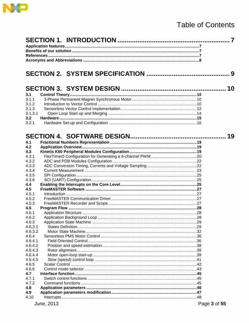
The features of the permanent magnet synchronous motor (high efficiency, high torque capability, high power density and durability) are attractive for using the PMSM in motion-control applications. The invention of the vector control algorithm of the AC motors came from the attempt to achieve an AC motor torque/speed characteristic similar to that characteristic of the separately excited DC motor. In the DC motor, the maximum torque is generated automatically because of the mechanical switch called the commutator that feeds current only to that coil, whose position is orthogonal to the direction of the magnetic flux generated by the stator permanent magnets or excitation coils. The PMSM has the inverse construction, the excitation is on the rotor, and the motor has no commutator. Due to the decomposition of the stator current into a magnetic field-generating part and a torque-generating part, it is possible to control these two components independently and to reach the required performance. In order to keep the constant desired torque, the magnetic field generated by the stator coils has to follow the rotor at the same “synchronous” speed. Therefore, to successfully perform the vector control, the rotor shaft position must be known and is one of the key variables in the vector control algorithm. For this purpose, either the mechanical position sensors are used (encoders, resolvers,..) or the position of the shaft is calculated (estimated) from the motor phase currents and voltage. This is is called “sensorless control”. Using the mechanical position sensors brings several benefits. The position is known over the entire speed range with the same precision and there is no need to compute highly mathematically intensive algorithms that estimate the rotor shaft position. Vector control with a position sensor can be implemented on less powerful microcontrollers, or the performance of the MCU can be used for other tasks. On the other hand, the cost of the mechanical sensor is a significant portion of the cost of the whole drive.

June, 2013 of 55

Figure 3-1 Synchronous machine and the main principle of the vector control

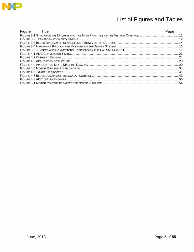
As already mentioned, the required torque is proportional to the q-portion of the orthogonal d,q- currents system. The d-portion reflects the generation of the rotor magnetic flux. Because there are permanent magnets mounted on the PMSM rotor, this current is usually kept at a zero level, unless the field weakening is performed in order to accelerate the motor above the nominal speed or while performing the MTPA algorithm. In such cases, the required d-current possesses a negative value. Therefore, the control process (regulation) is focused on maintaining the desired values of the d and q currents. Since the d,q system is referenced to the rotor, the measured stator currents have to be transformed from the 3-phase a,b,c stationary frame into the 2-phase d,q rotary frame before they enter the regulator block. At first, the Clarke transformation is calculated, which transforms the quantities from the 3-phase to 2-phase systems. Because the space vector is defined in the plane (2D), it is sufficient to describe it in the 2-axis (alpha, beta) coordinate system. Consequently, the result of the transformation into the 2-phase synchronous frame (Park transformation) is two DC values – the d,q currents. It is much easier to regulate two DC variables than two variables changing in time. The following picture shows the transformation sequencing.

June, 2013 of 55

Figure 3-2 Transformation sequencing

3.1.3 Sensorless vector control implementation

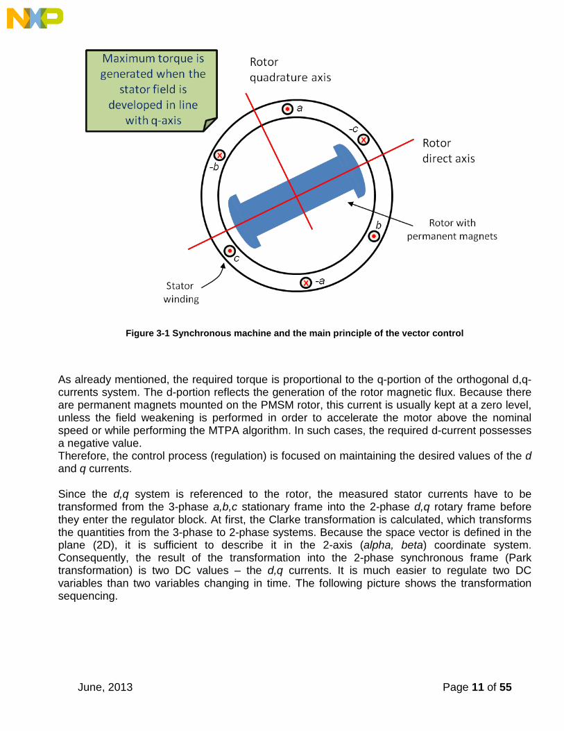
Figure 3-3 shows a block diagram of the vector control algorithm with sensorless position estimation. The aim of this control is to regulate the motor speed at a predefined level. The speed command value is set by a high level control. The algorithm is executed in two control loops. The fast inner control loop is executed within a hundred µsec period. The slow outer control loop is executed within a period of an msec. The fast control loop executes two independent current control loops. They are the direct and quadrature-axis current (isd , isq) PI controllers. The direct-axis current is used to control the rotor magnetizing flux. The quadrature-axis current corresponds to the motor torque. The current PI controllers’ outputs are summed with the corresponding d and q axis components of the decoupling stator voltage. Thus, the desired space vector for the stator voltage is obtained and then applied to the motor. The fast control loop executes all the necessary tasks to be able to achieve an independent control of the stator current components. These include:

• Three-phase current reconstruction • Forward Clarke transformation • Forward and backward Park transformations • Rotor magnetizing flux position evaluation • DC-bus voltage ripple elimination • Space vector modulation (SVM)

Furthermore, algorithims for rotor position estimation are also executed in the fast control loop: • Forward Park transformation for currents and voltages • Back-EMF observer • Tracking observer • Moving average filter

June, 2013 of 55

• Merging algorithm for smooth transition from open loop start-up to speed-close loop operation

The slow control loop executes the speed controller, field weakening control (if employed in the application) and lower priority control tasks. The PI speed controller output sets a reference for the torque producing quadrature axis component of the stator current iq_req. The flux producing current id_req is maintained at zero, because the magnetizing flux is generated by permanent magnets on the rotor. In the case when the field weakening is implemented in the application in order to reach higher than the nominal speed, then the value of the id_req current acquires negative values. Thus it is acting against the flux of the rotor permanent magnets. To achieve the goal of PM synchronous motor control, the algorithm uses feedback signals. The essential feedback signals are 3-phase stator current and stator voltage. For correct operation, the presented control structure estimates the rotor shaft position from the phase currents and voltages employing advanced position estimation algorithms, Back-EMF observer, and the Tracking observer. The back-EMF observer is based on the mathematical model of the synchronous motor with an extended electro-motive force function, which is realized in the estimated quasi synchronous reference frame. The back-EMF observer detects the generated motor voltages induced by the permanent magnets. A tracking observer uses the back-EMF signals to calculate the position and speed of the rotor. Since the back-EMF force is depending on the value of the angular speed of the motor, at the low-speed drive operation the output of the algorithm does not provide accurate position information. Therefore, in this application, the motor runs in the open-loop mode with forced rotor position values until the motor reaches 10% of its nominal speed. The merging algorithm then allows smooth transition from open-loop mode to speed closed-loop control without any torque ripples. During the open loop start-up the motor operates with limited output torque. When the drive application requires full torque at the motor start-up, you must use an additional method for position estimation that can detect the rotor position at stand still and low-speed operation. The description of the advanced position estimation algorithms can be found in the User’s guide [5] and in the DRM110 [2]. The merging algorithm will be described in the following text.

June, 2013 of 55

Figure 3-3 Block diagram of sensorless PMSM vector control

As seen from the block diagram shown in Figure 3-3, the algorithm of PMSM vector control is represented as a chain of functions; outputs of one function serve as inputs to the other functions. Each body of the functions contains mathematical equations, not involving the peripherals. In order to speed up the development of any motor control applications, these motor control functions, together with some commonly used mathematic algorithms, such as trigonometric functions, controllers, or limitations and digital filters, were put into one set and they create the Motor Control Library. The motor control libraries are available for some Freescale MCU platforms, optimized for each platform in order to maximize the utilization of available core features. The functions were tested and are well documented. Therefore, building the motor control application is, for the developer, simplified. The description of the libraries’ functions can be found in [4].

3.1.3.1 Open-loop start up and merging As mentioned, the output of the back-EMF observer does not provide reliable values at low speed motor operation. It is obvious from one of the motor operation fundamentals: at the zero speed there is no back-EMF generated. For this reason, the motor spins in the open-loop mode. The output of the speed regulator is disconnected and required startup current iq_req_startup is kept on constant level. The value of the startup current has to be carefully tuned. It has to be high

June, 2013 of 55

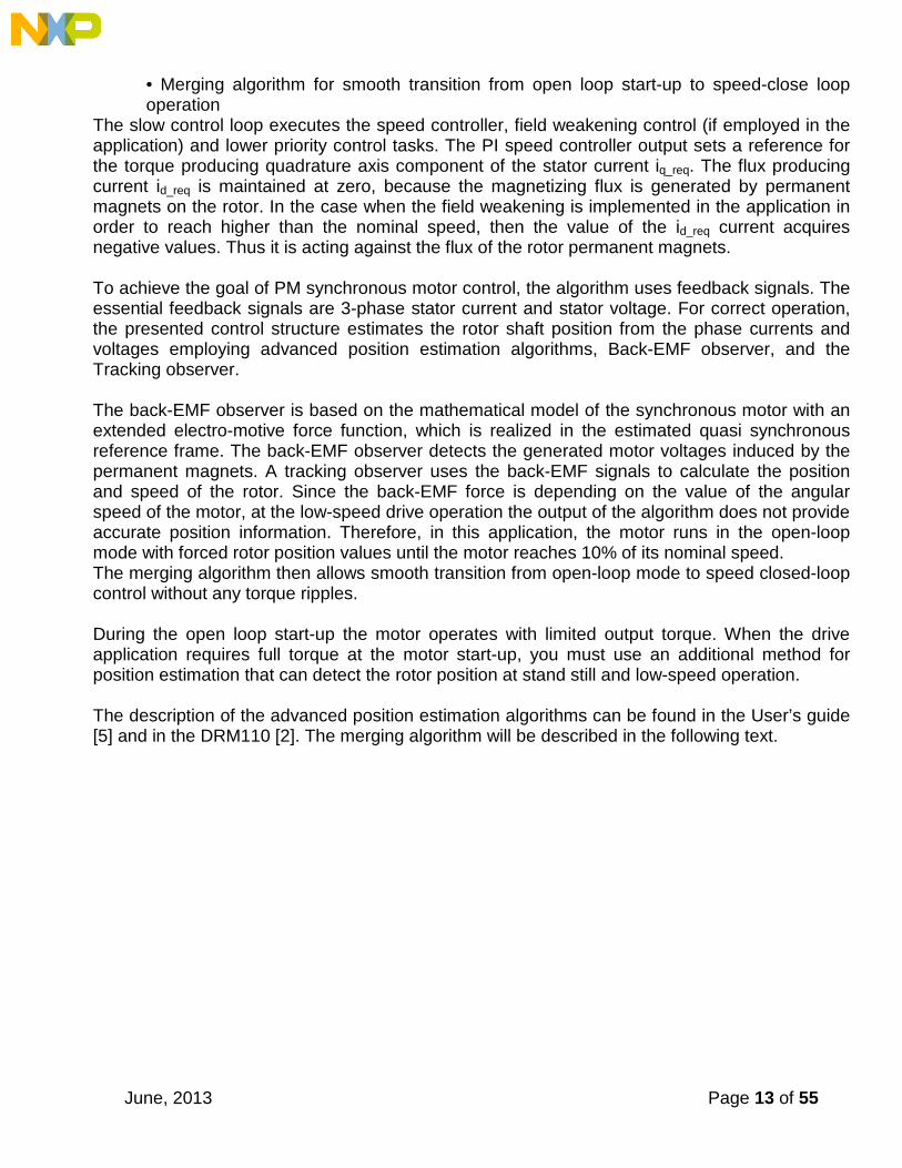
enough in order to put the rotor into the motion, but not too high when there could be observed speed oscillations during the transition to speed closed-loop operation. After a non-zero value of required speed is entered, the speed ramp block provides prescribed acceleration dynamic of the motor by smoothly increasing its output value. The required speed value then enters the integrator block, which gives the generated open-loop position of the rotor. This is essential to the performance of the vector control algorithm. This strategy moves the motor up to the speed threshold, when the output of the back-EMF observer algorithm is giving confident results of the rotor position and the speed. Because the open loop values of speed and position are not equal to estimated ones, direct switching the feedback from open loop to estimated values causes torque and speed ripple. A merging process assures smooth, torque and speed ripple-free transition from the open-loop startup to full sensorless speed closed loop control. The crossover merge function with weight coefficient aM is used to determine the position feedback signals. During the merging process the aM coefficient is changing its value from 0 to 1.

Figure 3-4 Crossover function with weight coefficient aM

The lower speed limit of crossover function (ωM1) is found through experimentation by evaluating the accuracy limits of the estimated values. The upper speed limit (ωM2) is set in such a way that the merging process of the position will be performed during less than one electrical revolution. The equation 3-1 shows the mathematical expression of the merging process for the position.

𝝑𝑭𝑩𝑪𝑲 = (𝟏 − 𝒂𝑴)𝝑𝑶𝑷𝑬𝑵_𝑳𝑶𝑶𝑷 + 𝒂𝑴 × 𝝑𝑬𝑺𝑻𝑰𝑴 Equation 3-1

After the merging process is finished (aM = 0), the equations above are no longer computed, and estimated values of position and speed feedback are directly fed into the control process.

3.2 Hardware

The hardware solution of the PMSM Sensorless Vector Control on Kinetis is built on Freescale’s Tower rapid prototyping system. It consists of the following modules:

• Tower Elevator Modules (TWR-ELEV) • Kinetis K60 Tower System Module (TWR-K60D100N)

June, 2013 of 55

• Low-voltage 3-phase Motor Control Tower System Module (TWR-MC-LV3PH) with included motor

• Tower Serial Module (TWR-SER) All modules of the Tower system are available for order via the Freescale web page or from distributors, so the user can easily build the hardware platform for which the application is targeted.

3.2.1 Hardware set up and configuration

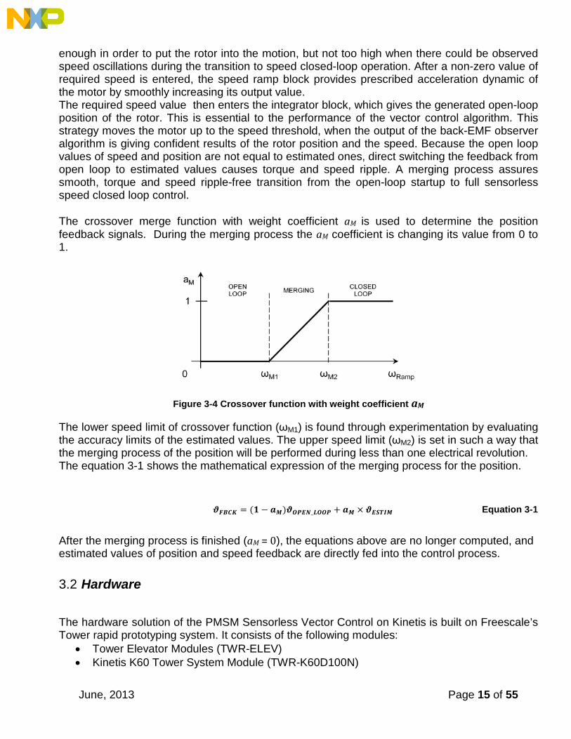
Building the system using the modules of the Tower system is not difficult. The peripheral modules and the MCU module are plugged into the elevator connectors, while the white stripe on the side of the module boards determines the orientation to the Functional elevator (the elevator with the mini USB connector, power supplies and the switch); see the following Figure 3-4.

Figure 3-4 Hardware built on the modules of the Tower system

The MCU board should be placed on the top of the Tower system, so the user’s buttons are easily accessible.

June, 2013 of 55

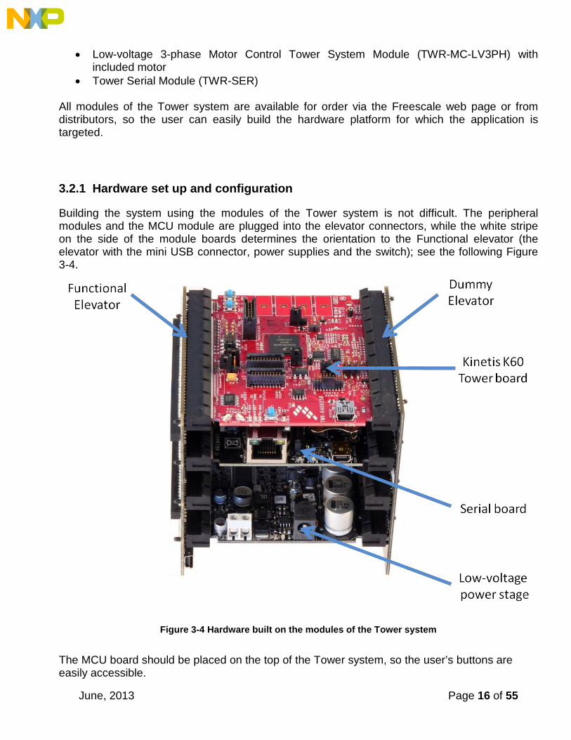
It is necessary to configure the Tower 3-phase low-voltage power stage. The jumper settings are listed in the following table, and the jumper positions are highlighted in Figure 3-5. See also the user’s manual [11] for more details (e.g. hardware overcurrent threshold setting) of the Tower low-voltage power stage. Table 3-1 Jumper settings of TWR-MC-LV3PH board

Jumper # Setting Note J2 VDDA Source Select 1-2 Internal analog power supply J3 VSSA Source Select 1-2 Internal analog power supply J10 AN6 Signal Select 1-2 Phase C current signal J11 AN5 Signal Select 1-2 Phase B current signal J12 AN2 Signal Select 1-2 Phase A current signal

Figure 3-5 Jumpers and connectors positions on the TWR-MC-LV3PH

Table 3-2 shows the signal assignment of the motor connector of the TWR-MC-LV3PH. Table 3-2 Motor and encoder connectors on the TWR-MC-LV3PH

Connector Pin# Description Motor connector 1 Motor phase A

June, 2013 of 55

J5 2 Motor phase B 3 Motor phase C

Warning for Revision “B” of the TWR-MC-LV3PH

Do not plug any other cables into the Tower system except for the power supply cable and serial communication cable. Do not connect any USB cable to the Tower system while the power is applied to the power stage module TWR-MC-LV3PH. The demo system can be powered only via the Tower Low Voltage Power Stage. Connecting a USB cable to the Tower Elevator Module could cause damage to the Kinetis K60. See Errata for the revision “B” of the TWR-MC-LV3PH on how to correctly operate the board. The motor used in the reference design is part of the TWR-MC-LV3PH kit. It is a BLDC motor with trapezoidal shape of the back-EMF voltage, with salient poles on the stator. This difference from the PM synchronous motor has distributed winding on the stator, forming the sinusoidal shape of the magnetic field. The construction of a rotor is the same for both types of motors (salient poles on the shaft). Even though the vector control algorithm was originally developed for PM synchronous motor assuming sinusoidal shape of the magnetic field, it is possible to employ the same control strategy for the BLDC motor. The performance will not be optimal, but the drive will possess less audible noise compared to a traditional six-step commutation control. The main benefit is that the customer can learn and adopt sensorless vector control on a cost effective hardware solution. The motor has the following specification: Table 3-3 Specification of the motor

Motor specification

Manufacturer name Linix Type 45ZWN24-40 Nominal voltage (line-to-line) 24 V DC Nominal speed 4000 rpm Rated power 40 W

Motor model parameters

Stator winding resistance (line-to-line) 1 Ohm

Stator winding inductance d axis 775.8 μH

Stator winding inductance q axis 775.8 μH

Number of pole-pairs 2

NOTE:

June, 2013 of 55

The application parameters (speed PI controller and value of the startup current) are set for the motor that has a plastic circle (part of the kit) mounted on the shaft, otherwise speed oscillation might occur.

Section 4. Software design The application software was designed using the compiler IAR Embedded Workbench for ARM v. 6.40.2

4.1 Fractional numbers representation

As mentioned in a previous paragraph, in the development of the vector control algorithm software libraries were used (a Set of the General Maths and Motor Control Functions for the Cortex M4 Core). Most of the mathematical calculations were performed with the numbers represented in Q1.15 or Q1.31 signed fractional format, so all physical quantities were scaled to the <-1,1) interval. For more on the fractional format and variables scaling, see DRM105 [3].

4.2 Application overview

The application is real-time interrupt-driven with the background infinite loop handling the application states (Initialization, Run, Fault…) and FreeMASTER communication polling. There are two periodic interrupt service routines where the control process is executed. Their timing is given by the requirements of the vector control algorithm. The control process is composed of two control loops. The execution of the fast (current) control loop is performed in the ADC1 interrupt service routine, which is executed after the values of the sampled DC bus voltage and motor phase currents are put into the ADC result registers. The sampling instance is precisely defined by the hardware trigger of FlexTimer0 that is configured to generate six PWM signals of frequency 16 kHz. The PIT0 interrupt service routine is triggered every one millisecond. In this ISR, the speed is calculated as a position derivation and the speed controller (slow speed control loop) is calculated. The individual processes of the control routines are described in the following sections.

4.3 Kinetis K60 peripheral modules configuration

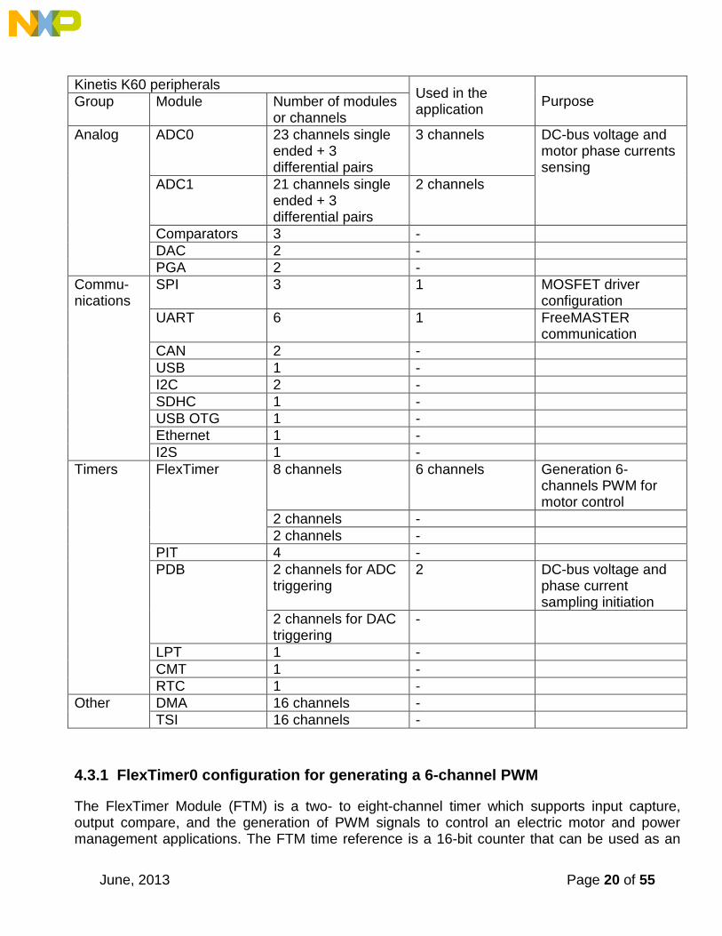
In this section, the configuration procedures of the peripherals used are described or referenced. On all devices of the Kinetis family, it is necessary to enable the system clock for the module before any access to the peripheral registers is performed. The modules are enabled by writing “1” to the particular bit in the System Clock Gate Control Register. Any write or read attempt to the peripheral register before enabling the clock for the particular peripheral module will yield a hard fault. Refer to [1] for a detailed description of each peripheral module. Table 4-1 shows an overview of the Kinetis K60 peripheral modules used by the application. The number of modules and module channels reflect a 144-pin package. Table 4-1 Kinetis K60 peripherals overview

June, 2013 of 55

Kinetis K60 peripherals Used in the

application Purpose Group Module Number of modules or channels

Analog ADC0 23 channels single ended + 3 differential pairs

3 channels

DC-bus voltage and motor phase currents sensing

ADC1 21 channels single ended + 3 differential pairs

2 channels

Comparators 3 - DAC 2 - PGA 2 -

Commu-nications

SPI 3 1 MOSFET driver configuration

UART 6 1 FreeMASTER communication

CAN 2 - USB 1 - I2C 2 - SDHC 1 - USB OTG 1 - Ethernet 1 - I2S 1 -

Timers FlexTimer 8 channels 6 channels Generation 6-channels PWM for motor control

2 channels - 2 channels -

PIT 4 - PDB 2 channels for ADC

triggering 2 DC-bus voltage and

phase current sampling initiation

2 channels for DAC triggering

-

LPT 1 - CMT 1 - RTC 1 -

Other DMA 16 channels - TSI 16 channels -

4.3.1 FlexTimer0 configuration for generating a 6-channel PWM

The FlexTimer Module (FTM) is a two- to eight-channel timer which supports input capture, output compare, and the generation of PWM signals to control an electric motor and power management applications. The FTM time reference is a 16-bit counter that can be used as an

June, 2013 of 55

unsigned or signed counter. On the Kinetis K60 there are three instances of FTM. One FTM has 8 channels, the other two FTMs have 2 channels. The procedure to configure the FlexTimer for generating a center-aligned PWM with dead time insertion is described in the application note AN3729 [6]. Because the referenced application note supports an earlier version (1.0) of the FlexTimer implemented on the ColdFire V1, and with respect to the hardware used (TWR-MC-LV3PH), there are a few differences in the configuration, as described below:

• Initially, it is necessary to enable the system clock for the FlexTimer module in the Clock Gating Control Register: SIM_SCGC6 |= SIM_SCGC6_FTM0_MASK;

• It is necessary to disable the write protection of some registers before they can be updated: FTM0_MODE |= FTM_MODE_WPDIS_MASK;

• It is advisable to enable the internal FlexTimer counter to run in debug mode: FTM0_CONF |= FTM_CONF_BDMMODE(3); While the HW debugging interface (jLink, Multilink…) is connected to the microcontroller, the MCU is in debug mode. This does not depend on whether the running code containing breakpoints or not.

• The PWM signals generated by the FlexTimer0 are directly connected to the MOSFET driver. Due to safety reasons, the input signals for the top transistors on the MOSFET driver used on the Tower low-voltage power stage have inversed polarity. Therefore, it is also necessary to set the right polarity of the PWM signals: FTM0_POL = FTM_POL_POL0_MASK |

FTM_POL_POL2_MASK | FTM_POL_POL4_MASK;

• The duty cycle is changed by changing the value of the FlexTimer Value registers. These registers are double-buffered, meaning that their values are updated not only by writing the number, but it is necessary to confirm the change by setting the Load Enable (LDOK) bit. This ensures that all values are updated at the same instance: FTM0_PWMLOAD = FTM_PWMLOAD_LDOK_MASK; It is necessary to write the LDOK bit every time the value registers are changed, not only at the initial stage of loading them with values, but with every update after the duty cycle value is computed in the vector control algorithm.

• As mentioned in section 4.3.4

FTM0_EXTTRIG |= FTM_EXTTRIG_INITTRIGEN_MASK;

, in the application, hardware triggering of the A/D converter is employed. The Initialization Trigger signal from the FlexTimer is used as the primary triggering signal, which is fed into the Programmable Delay Block that services the timing of the AD conversion initiation.

• Finally, the output pins of the MCU have to be configured in order to send the signals out of the chip. The assignment of signals to output pins is set in the Pin Control Register, while the available signals are listed in the Signal Multiplexing chapter of [1] and are package dependent. PORTC_PCR1 = PORT_PCR_MUX(4); // FTM0 CH0 PORTC_PCR2 = PORT_PCR_MUX(4); // FTM0 CH1 PORTC_PCR3 = PORT_PCR_MUX(4); // FTM0 CH2 PORTA_PCR6 = PORT_PCR_MUX(3); // FTM0 CH3 PORTA_PCR7 = PORT_PCR_MUX(3); // FTM0 CH4

June, 2013 of 55

PORTD_PCR5 = PORT_PCR_MUX(4); // FTM0 CH5 The port settings implemented in the application code reflect the hardware solution built on the Tower system modules.

4.3.2 ADC and PDB modules configuration

The on-chip ADC module is used to sample feedback signals (motor phase currents and DC bus voltage) that are necessary to successfully perform the vector control algorithm. The Programmable Delay Block closely cooperates with the ADC and serves as the hardware trigger for the sampling. In order to obtain a specified accuracy, it is necessary to perform a self-calibrating procedure of the ADC module before it is used in the application. The calibration process also requires a programmer’s intervention to generate the plus-side and minus-side gain calibration results and store them in the ADC plus-side gain and minus-side gain registers after the calibration function completes. The calibration has to be performed for both the ADC modules. After calibration, the ADC modules are configured to a 12-bit accuracy. The input clock of the ADC module is limited to 18 MHz according to the Kinetis K60 datasheet [9]. The CPU frequency is set to 100 MHz, so by using available prescaler value, the input clock to the ADC module is set to 12.5 MHz. That setting yields a conversion time of 2.2 µs. Finally, the hardware trigger has to be enabled in the Status and Control Register 2. The Programmable Delay Block (PDB) provides controllable delays from either an internal or an external trigger, or a programmable interval tick, to the hardware trigger inputs of the ADCs, so that a precise timing between ADC conversions is achieved. The PDB module has an internal counter that overflows on a modulo value. Because the input trigger comes periodically from the FTM0, the input clock source and the modulo value is set identically as for the FTM0 module. The values in the channel delay registers are set to generate triggers to start sampling the DC-bus voltage and the motor phase AD conversions. The PDB module on the K60 MCU allows 15 different input trigger sources. They are listed in the chapter “Chip configuration” in the section "PDB Configuration” in device reference manual [1]. Similarly, as for the FTM0, the LDOK bit has to be set in order to acknowledge the changes in the modulo and the delay registers.

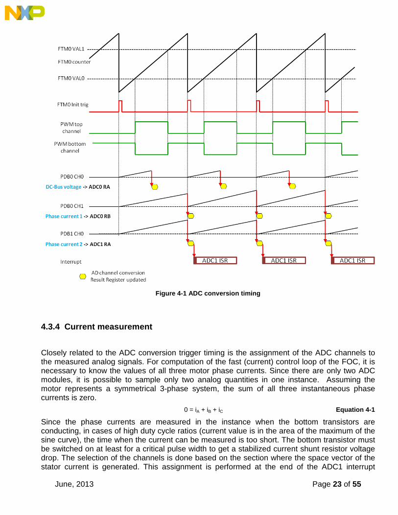
4.3.3 ADC conversion timing, currents and voltage sampling

The FlexTimer0 is configured to trigger an internal hardware signal when its counter is reset after overflow to the initialization value. This signal is fed into the Programmable Delay Block (PDB) that consequently triggers the AD conversion of the voltage and currents with a predefined delay. On the Kinetis K60 100 MHz MCU, two ADC modules are implemented. Each ADC module associates to one channel of the PDB module. Each ADC module has two result registers (two channels), and they correspond to two programmable pre-trigger delays of the PDB channels. It is possible to perform four AD conversions without requesting an interrupt (provided that the DMA is not used for data transfer). In this application, only 3 conversions need to be triggered without CPU intervention (two motor phase currents and the DC-Bus voltage). The following time diagram shows the modules interconnection and the ADC interrupt generation.

June, 2013 of 55

Figure 4-1 ADC conversion timing

4.3.4 Current measurement

Closely related to the ADC conversion trigger timing is the assignment of the ADC channels to the measured analog signals. For computation of the fast (current) control loop of the FOC, it is necessary to know the values of all three motor phase currents. Since there are only two ADC modules, it is possible to sample only two analog quantities in one instance. Assuming the motor represents a symmetrical 3-phase system, the sum of all three instantaneous phase currents is zero.

0 = iA + iB + iC Equation 4-1

Since the phase currents are measured in the instance when the bottom transistors are conducting, in cases of high duty cycle ratios (current value is in the area of the maximum of the sine curve), the time when the current can be measured is too short. The bottom transistor must be switched on at least for a critical pulse width to get a stabilized current shunt resistor voltage drop. The selection of the channels is done based on the section where the space vector of the stator current is generated. This assignment is performed at the end of the ADC1 interrupt

June, 2013 of 55

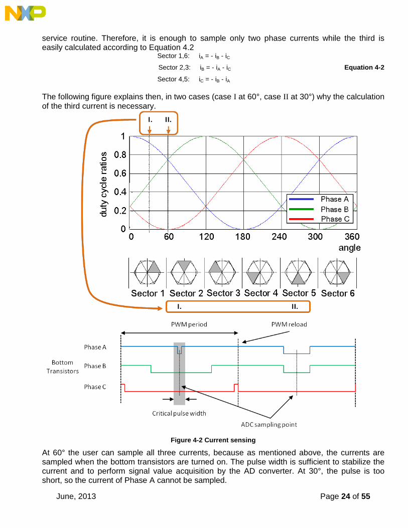
service routine. Therefore, it is enough to sample only two phase currents while the third is easily calculated according to Equation 4.2

Sector 1,6: iA = - iB - iC

Sector 2,3: iB = - iA - iC Equation 4-2

Sector 4,5: iC = - iB - iA

The following figure explains then, in two cases (case I at 60°, case II at 30°) why the calculation of the third current is necessary.

Figure 4-2 Current sensing

At 60° the user can sample all three currents, because as mentioned above, the currents are sampled when the bottom transistors are turned on. The pulse width is sufficient to stabilize the current and to perform signal value acquisition by the AD converter. At 30°, the pulse is too short, so the current of Phase A cannot be sampled.

June, 2013 of 55

4.3.5 SPI configuration

The SPI interface is used in the application for communication between the intelligent MOSFET gate driver MC33937 and the K60 MCU. The MC33937 gate driver is placed on the Tower low-voltage power module and serves to drive the high-side and low-side MOSFET transistors of the 3-phase inverter. In the application, the initialization of the MC33937 has to be performed to set the dead time. During the motor run there is also periodic checking of the status register of the driver, in order to provide information on the latched faults. The MC33937 driver requires precise timing of the SPI signals. It is not possible to use the default setting of the SPI module on the MCU. The exact timing of the SPI signals is listed in [7].

4.3.6 SCI (UART) configuration

The SCI is used in the application for the communication between the master system and the embedded application. A master system is the notebook or the PC where the FreeMASTER software is installed in order to control the application and visualization of its state. On the Kinetis K60, there are six UART modules implemented. The UART3 is used because the hardware solution is based on the Tower modules. The communication speed is set to 19200 Bd, and in fact, it is limited by the USB-to-Serial cable used. The use of direct RS232 connection between the PC and the embedded side allows users to increase the communication speed to 115200 Bd. The module configuration is performed in the FreeMASTER software driver included in the project.

4.4 Enabling the interrupts on the core level

The interrupt request enabled on the peripheral module must also be enabled on the core level, otherwise the interrupt request will not be generated. The process is not straightforward and the necessary information is spread over several documents. In order to help the user to enable any interrupt while enhancing the application to other features, the process of setting up the PIT interrupt is described in this section as an example. The interrupt request on the module level is enabled by writing “1” to the TIE bit of the Timer Control Register: PIT_TCTRL0 |= PIT_TCTRL_TIE_MASK; Now, it is necessary to find out the number of the interrupt and the IRQ vector. Both values can be found in the K60 Sub-Family Reference Manual [1] in the section 3.2.2.3 “Interrupt channel assignments”. For the PIT channel 1 interrupt, the interrupt vector is 84 and the interrupt number is 68. This is always 16 less than the vector number, because the first 16 interrupt vectors are ARM core system handler exception vectors. The next step is to redefine the vector pointer in the “vectors.h” file from the default ISR to the function that contains the code to be executed after an interrupt is generated. Replace

#define VECTOR_084 default_isr with

#define VECTOR_084 PIT_CH0_ISR_Handler and add at the end of the file:

June, 2013 of 55

extern void PIT_CH0_ISR_Handler(void); because the ISR is defined in the other file (e.g. in “main.c”). Next, set-up the ARM core NVIC register. Each interrupt vector must be independently enabled or disabled by setting the corresponding bit in the complementary pair of registers, the Interrupt Set-Enable Register (NVIC_ISERx) or the Interrupt Clear-Enable Register (NVIC_ICERx). NVIC_ISER0 contains the enable bits for IRQ numbers 0 through 31, NVIC_ISER1 contains the enable bits for IRQ 32 through 63, and so on. To enable the PIT channel 0 interrupt (interrupt number 68), it is necessary to write 0x00000010 (b10000) to the NVIC_ISER2 register. It is an advisable approach to clear any pending interrupt before it is enabled. This is usually not necessary right after the reset when the MCU initialization is performed, but during the program execution when certain a interrupt is disabled and later re-enabled. Sometimes if an interrupt flag has been set before the interrupt was enabled, the interrupt controller might generate an unhandled exception fault if the interrupt flag has not been cleared before: NVICICPR2 = 0x00000010; // clear pending interrupts first NVICISER2 = 0x00000010; // enable the PIT CH0 interrupt

NOTE: The ARM document [8] indicates that the registers have an underscore between NVIC and ISER (NVIC_ISER1). However, in the current header files used in the application, the NVIC register names do not have the underscore (NVICISER1 or NVICICPR1). NVIC interrupts are prioritized by updating an 8-bit field within the 32-bit NVIC_IPRx registers. Macros contained in the Kinetis K60 header file used in the project make setting the priority of the interrupt simpler. The number of the interrupt is used as one of the parameters of the NVIC_IP macro. The assigned value then determines the priority (the higher the number, the higher the priority of the interrupt). If the interrupt priority is not specified explicitly, the lower the number of the interrupt vector, the higher priority the interrupt has by default. On the Kinetis K family there are 16 levels of interrupt priority implemented. However, the priority is set in the four MSBs of the 8-bit field: NVIC_IP(68) = 0xF0; //set the highest priority for PIT ch. 0 interrupt. The next step is to enable the interrupts globally by clearing a 1-bit special-purpose mask register PRIMASK. The PRIMASK is cleared to 0 by the execution of the instruction CPSIE i : In the application this is defined as the macro: #define EnableInterrupts asm(" CPSIE i "); Finally, the interrupt service routine has to be defined “PIT_CH0_ISR_Handler” and inside the body of the function, the source of the interrupt must be cleared in order to leave the interrupt service routine. For the PIT channel 0 interrupt, it means that the interrupt flag is cleared by writing “1” to the TIF bit of the Timer Flag Register: PIT_TFLG0 = PIT_TFLG_TIF_MASK;

June, 2013 of 55

4.5 FreeMASTER software

4.5.1 Introduction

The FreeMASTER software was designed to provide a debugging, diagnostic, and demonstrational tool for the development of algorithms and applications. Moreover, it is very useful for tuning the application for different power stages and motors, because almost all of the application parameters can be changed via the FreeMASTER interface. The FreeMASTER consists of a component running on a PC and another part running on the target controller. Different communication interfaces are supported (RS-232, USB, Ethernet, OSBDM…) and the work on improvements and support for new families of microcontrollers is still in progress. In the application, the RS232 interface is used because it represents minimal communication overhead that has to be handled by the MCU, and requires no interrupts (working in polling mode), which is important for motor control applications. A detailed users’ guide of FreeMASTER software, with useful hints for using it to develop a motor control application can be found in AN1948 [10].

4.5.2 FreeMASTER communication driver

On the MCU side, the FreeMASTER software driver is included in the project file structure. It is a set of files supporting real-time data capture (Scope, Recorder) and handling the communication protocol. There are some functions that are unique for each MCU family, therefore FreeMASTER is issued for each MCU family separately. In the “freemaster_cfg.h” file, the user can perform settings related to the communication and to the data buffer. In the file are defined macros for conditional and parameter compilation. The FreeMASTER driver does not perform any initialization or configuration of the SCI module it uses to communicate. The communication between the MCU and the PC side can be performed with the help of the interrupt, or via periodic calling of the polling function. For a motor control application, it is preferred to use the polling mode. Both the communication and protocol decoding are handled in the application background loop. The polling mode requires a periodic call of the FMSTR_Poll() function in the application main.

4.5.3 FreeMASTER recorder and scope

The recorder is a part of the FreeMASTER software that is able to sample the application variables at a specified sample rate. The samples are stored in a buffer and read by the PC via an RS-232 serial port. The sampled data can be displayed in a graph, or the data can be stored. The recorder behaves as a simple on-chip oscilloscope with trigger/pre-trigger capabilities. The size of the recorder buffer and the FreeMASTER recorder time base can be defined in the “freemaster_cfg.h” configuration file. The recorder routine must be called periodically from the loop in which you want to take the samples. The following line must be added to the loop code:

/* Freemaster recorder */ FMSTR_Recorder();

In this application, the FreeMASTER recorder is called from the ADC1 interrupt, which creates a 63 μs time base for the recorder function. Buffered data is transferred to the PC side after the trigger condition is met.

June, 2013 of 55

The FreeMASTER scope is a similar visualization tool to the recorder, but the data from the embedded side is downloaded in real-time. The sampling rate is limited by the speed of the communication protocol and also influenced by the number of displayed variables. It is usually used for waveforms visualization of slow transient phenomena, such as the speed profile during motor acceleration.

4.6 Program flow

4.6.1 Application structure

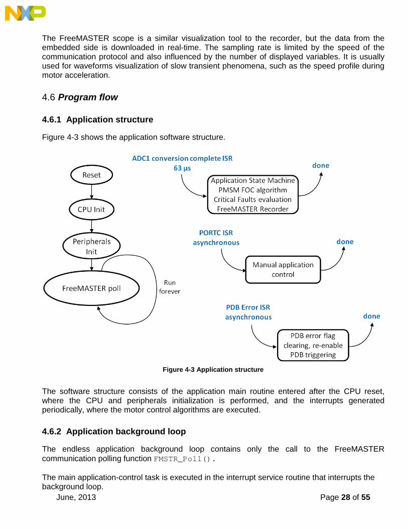
Figure 4-3 shows the application software structure.

Figure 4-3 Application structure

The software structure consists of the application main routine entered after the CPU reset, where the CPU and peripherals initialization is performed, and the interrupts generated periodically, where the motor control algorithms are executed.

4.6.2 Application background loop

The endless application background loop contains only the call to the FreeMASTER communication polling function FMSTR_Poll(). The main application-control task is executed in the interrupt service routine that interrupts the background loop.

June, 2013 of 55

4.6.3 Application state machine

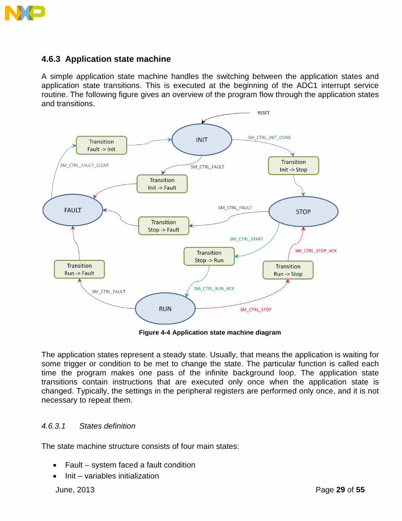
A simple application state machine handles the switching between the application states and application state transitions. This is executed at the beginning of the ADC1 interrupt service routine. The following figure gives an overview of the program flow through the application states and transitions.

Figure 4-4 Application state machine diagram

The application states represent a steady state. Usually, that means the application is waiting for some trigger or condition to be met to change the state. The particular function is called each time the program makes one pass of the infinite background loop. The application state transitions contain instructions that are executed only once when the application state is changed. Typically, the settings in the peripheral registers are performed only once, and it is not necessary to repeat them.

4.6.3.1 States definition The state machine structure consists of four main states:

• Fault – system faced a fault condition • Init – variables initialization

June, 2013 of 55

• Stop – system is initialized and waiting for the Run command • Run – system is running; can be stopped by the Stop command

There are transition functions between these state functions:

• Init -> Stop – initialization has been done, the system is entering the Stop state • Stop -> Run – the Run command has been applied, the system is entering the Run state

if the Run command has been acknowledged • Run -> Stop – the Stop command has been applied, the system is entering the Stop state

if the Stop command has been acknowledged • Fault -> Init – fault flag has been cleared, the system is entering the Init state • Init, Stop, Run -> Fault – a fault condition has occurred, the system is entering the Fault

state.

The state machine structure uses the following flags to switch between the states: • SM_CTRL_INIT_DONE when this flag is set the system goes from the Init to the Stop

state. • SM_CTRL_FAULT – when this flag is set the system goes from any state to the Fault

state. • SM_CTRL_FAULT_CLEAR – when this flag is set the system goes from the Fault state to

the Init state. • SM_CTRL_START – this flag informs the system that there is a command to go from the

Stop state to the Run state. The transition function is called, but the action must be acknowledged due to the amount of time it may take before the system is ready to be turned on.

• SM_CTRL_RUN_ACK – this flag acknowledges that the system can proceed from the Stop state to the Run state.

• SM_CTRL_STOP – this flag informs the system that there is a command to go from the Run state to the Stop state. The transition function is called, but the action must be acknowledged because it may take time to properly turn off the system.

• SM_CTRL_STOP_ACK – this flag acknowledges that the system can proceed from the Run state to the Stop state.

This structure is implemented in the state_machine.c .h files. The state machine structure is as follows: /* State machine control structure */ typedef struct { SM_APP_STATE_FCN_T const* psState; /* State functions */ SM_APP_TRANS_FCN_T const* psTrans; /* Transition functions */ SM_APP_CTRL uiCtrl; /* Control flags */ SM_APP_STATE_T eState; /* State */ } SM_APP_CTRL_T; There are four components:

June, 2013 of 55

• psState – pointer to the user state machine functions. The particular state machine function from this table is called when the state machine is in that state.

• psTrans – pointer to the user transient functions. The particular transient function is called when the system goes from one state to another.

• uiCtrl – this variable is used to control the state machine behavior using the above mentioned flags.

• eState – this variable determines the actual state of the state machine

The user state machine functions are defined in the following structure: /* User state machine functions structure */ typedef struct { PFCN_VOID_VOID Fault; PFCN_VOID_VOID Init; PFCN_VOID_VOID Stop; PFCN_VOID_VOID Run; } SM_APP_STATE_FCN_T; The user transient state machine functions are defined in the following structure: /* User state-transition functions structure*/ typedef struct { PFCN_VOID_VOID FaultInit; PFCN_VOID_VOID InitFault; PFCN_VOID_VOID InitStop; PFCN_VOID_VOID StopFault; PFCN_VOID_VOID StopInit; PFCN_VOID_VOID StopRun; PFCN_VOID_VOID RunFault; PFCN_VOID_VOID RunStop; } SM_APP_TRANS_FCN_T; The control flag’s variable has the following definitions: typedef unsigned short SM_APP_CTRL; /* State machine control command flags */ #define SM_CTRL_NONE 0x0 #define SM_CTRL_FAULT 0x1 #define SM_CTRL_FAULT_CLEAR 0x2 #define SM_CTRL_INIT_DONE 0x4 #define SM_CTRL_STOP 0x8 #define SM_CTRL_START 0x10 #define SM_CTRL_STOP_ACK 0x20 #define SM_CTRL_RUN_ACK 0x40 The state identification variable has the following definitions: /* Application state identification enum */ typedef enum { FAULT = 0,

June, 2013 of 55

INIT = 1, STOP = 2, RUN = 3, } SM_APP_STATE_T; The state machine must be periodically called from the code using the following inline function. This function input is the pointer to the above-described state machine structure, which is declared and initialized in the code where the state machine is called: /* State machine function */ extern inline void SM_StateMachine(SM_APP_CTRL_T *sAppCtrl) { gSM_STATE_TABLE[sAppCtrl -> eState](sAppCtrl); }

4.6.3.2 Motor state machine The motor state machine is based on the main state machine structure. The Run state sub-states have been added on top of the main structure to control the motor properly. These are the descriptions of the main states’ user functions:

• Fault – system faced a fault condition, and waits until the fault flags are cleared. The dc bus voltage is measured.

• Init – variables initialization • Stop – system is initialized and waiting for the Run command. The PWM output is

disabled. The dc bus voltage is measured. • Run – system is running and can be stopped by the Stop command. The Run sub-state

functions are called from here.

There are transition functions between these state functions: • Init -> Stop – blue LED is lit on the K60 tower board • Stop -> Run – duty cycle is initialized to 50 %; the PWM output is enabled. The current

ADC channels are initialized. The Calib sub-state is set as the initial Run sub-state. • Run -> Stop – the Stop command has been applied, the system is entering the Stop state

if the Stop command has been acknowledged. The system does not go directly to Stop if the system is in certain Run sub-states.

• Fault -> Init – nothing is processed in this function • Init, Stop -> Fault – the PWM output is disabled. • Run -> Fault – certain current and voltage variables are zeroed. The PWM output is

disabled.

The Run sub-states are called when the state machine is in the Run state. The Run sub-state functions are as follows:

• Calib – the current channels ADC offset calibration is performed. The dc bus voltage is measured. The PWM is set to 50 % and its output is enabled.

• Ready – the PWM is set to 50 % and its output is enabled. The current is measured and the ADC channels, set up. Certain variables are initialized.

June, 2013 of 55

• Align – The current is measured and the ADC channels, set up. The rotor alignment algorithm is called. The PWM is updated. After the alignment time expiration, the system is switched to Startup. The dc bus voltage is measured.

• Startup – The current is measured and the ADC channels, set up. The BEMF observer algorithm is called to estimate the speed and position. The FOC algorithm is called. The PWM is updated. The dc bus voltage is measured and filtered. The open-loop start-up algorithm is called. The estimated speed is filtered.

• Spin – The current is measured and the ADC channels, set up. The BEMF observer algorithm is called to estimate the speed and position. The FOC algorithm is called. The PWM is updated. The motor spins. The dc bus voltage is measured. The estimated speed is filtered. The speed ramp and the speed PI controller algorithm is called. The speed command is evaluated.

• Freewheel – the PWM output is disabled and the module is set to 50 %. The current is measured and the ADC channels, set up. The dc bus voltage is measured. The system waits in this sub-state for certain time which is given due to rotor inertia, it means to wait until the rotor stops itself. Then the system evaluates the conditions and proceeds into one of these sub-states: Align or Ready.

The Run sub-states have also the transition functions that are called in between the sub-states’ transition. The sub-state transition functions are as follows:

• Calib -> Ready – calibration done, entering the Ready state. • Ready -> Align – non-zero speed command; entering the Align state. Certain variables

are initialized (voltage, speed, position). The alignment time is set up. • Align -> Ready – zero speed command; entering the Ready state. Certain voltage and

current variables are zeroed. The PWM is set to 50 %. • Align -> Startup – alignment done; entering the Startup state. The filters and control

variables are initialized. The PWM is set to 50 %. • Startup -> Spin – start-up successful; entering the Spin state. • Startup -> Freewheel – no action is done. Can be used to handle the start-up fail

condition for more robust application • Spin -> Freewheel – zero speed command; entering the Freewheel state. Certain

variables are initialized (voltage, speed, position). The freewheel time is set up. • Freewheel -> Ready – zero-speed command; entering the Ready state. The PWM output

is enabled. • Freewheel -> Align – non-zero speed command; entering the Align state. The PWM

output is enabled. Certain variables are initialized (voltage, speed, position). The alignment time is set up.

June, 2013 of 55

Figure 4-5 Motor Run sub-state diagram

The implementation of this structure of motor state machine is made in the M1_statemachine.c .h. The main motor state-machine structure is as follows: The main states’ user function prototypes: static void M1_StateFault(void); static void M1_StateInit(void); static void M1_StateStop(void); static void M1_StateRun(void); The main states’ user transient function prototypes: static void M1_TransFaultInit(void); static void M1_TransInitFault(void); static void M1_TransInitStop(void); static void M1_TransStopFault(void); static void M1_TransStopInit(void); static void M1_TransStopRun(void); static void M1_TransRunFault(void); static void M1_TransRunStop(void); The main states functions table initialization: /* State machine functions field */ static const SM_APP_STATE_FCN_T msSTATE = {M1_StateFault, M1_StateInit, M1_StateStop, M1_StateRun}; The main state transient functions table initialization: /* State-transition functions field */

June, 2013 of 55

static const SM_APP_TRANS_FCN_T msTRANS = {M1_TransFaultInit, M1_TransInitFault, M1_TransInitStop, M1_TransStopFault, M1_TransStopInit, M1_TransStopRun, M1_TransRunFault, M1_TransRunStop}; Finally, the main state machine structure initialization: /* State machine structure declaration and initialization */ SM_APP_CTRL_T gsM1_Ctrl = { /* gsM1_Ctrl.psState, User state functions */ &msSTATE, /* gsM1_Ctrl.psTrans, User state-transition functions */ &msTRANS, /* gsM1_Ctrl.uiCtrl, Deafult no control command */ SM_CTRL_NONE, /* gsM1_Ctrl.eState, Default state after reset */ INIT }; Similarly, the Run sub-state machine is declared. The Run sub-state identification variable has the following definitions: typedef enum { CALIB = 0, READY = 1, ALIGN = 2, STARTUP = 3, SPIN = 4, FREEWHEEL = 5, } M1_RUN_SUBSTATE_T; /* Run sub-states */ For the Run sub-states, the following set of user functions is defined: static void M1_StateRunCalib(void); static void M1_StateRunReady(void); static void M1_StateRunAlign(void); static void M1_StateRunStartup(void); static void M1_StateRunSpin(void); static void M1_StateRunFreewheel(void); static void M1_StateRunCalibSlow(void); static void M1_StateRunReadySlow(void); static void M1_StateRunAlignSlow(void); static void M1_StateRunStartupSlow(void); static void M1_StateRunSpinSlow(void); static void M1_StateRunFreewheelSlow(void); The Run sub-states’ user transient function prototypes: static void M1_TransRunCalibReady(void); static void M1_TransRunReadyAlign(void); static void M1_TransRunAlignStartup(void); static void M1_TransRunAlignReady(void); static void M1_TransRunStartupSpin(void); static void M1_TransRunStartupFreewheel(void); static void M1_TransRunSpinFreewheel(void);

June, 2013 of 55

static void M1_TransRunFreewheelAlign(void); static void M1_TransRunFreewheelReady(void); The Run sub-states functions table initialization: /* Sub-state machine functions field (in pmem) */ static const PFCN_VOID_VOID mM1_STATE_RUN_TABLE[6] =

{M1_StateRunCalib, M1_StateRunReady, M1_StateRunAlign, M1_StateRunStartup, M1_StateRunSpin, M1_StateRunFreewheel};

The state machine is called from the interrupt service routine, as mentioned in a previous chapter. The method to call the state machine is: /* StateMachine call */ SM_StateMachine(&gsM1_Ctrl); Inside the user Run state function, the sub-state functions are called as follows: /* Run sub-state function */ mM1_STATE_RUN_TABLE[meM1_StateRun](); where the parameter meM1_StateRun identifies the Run sub-state.

4.6.4 Sensorless PMS motor control

The application controls one motor in sensorless mode. It is designed so that enhancing the application to drive a second motor (if CPU performance is adequate and the device possesses two motor-control PWM timers) does not require substantial modification. For the second motor, an additional application state machine is required (which can be the same as for the first motor), while the control process uses the same routine. The inputs to this routine are the particular motors’ structures. This approach saves the necessary program ROM in the application. The following sections are dedicated to the motor control algorithm pieces.

4.6.4.1 Field oriented control The field oriented control (FOC alias vector control) theory is described in the chapter 3.1.2 (Introduction to Vector Control) and in referenced literature. A description of the FOC code implementation follows. The FOC has been optimized into one function which has one input/output pointer to a structure. The prototype of the function is as follows: void MCSTRUC_FocPMSMCurrentCtrl(MCSTRUC_FOC_PMSM_T *psFocPMSM) The structure referred to by the input/output structure pointer is defined as follows: typedef struct {

June, 2013 of 55

GFLIB_CONTROLLER_PIAW_P_T sIdPiParams; /* Id PI controller parameters */ GFLIB_CONTROLLER_PIAW_P_T sIqPiParams; /* Iq PI controller parameters */ MCLIB_3_COOR_SYST_T sIABC; /* Measured 3-phase current */ MCLIB_2_COOR_SYST_ALPHA_BETA_T sIAlBe; /* Alpha/Beta current */ MCLIB_2_COOR_SYST_D_Q_T sIDQ; /* DQ current */ MCLIB_2_COOR_SYST_D_Q_T sIDQReq; /* DQ required current */ MCLIB_2_COOR_SYST_D_Q_T sIDQError; /* DQ current error */ MCLIB_3_COOR_SYST_T sDutyABC; /* Applied duty cycles ABC */ MCLIB_2_COOR_SYST_ALPHA_BETA_T sUAlBeReq; /* Required Alpha/Beta voltage */ MCLIB_2_COOR_SYST_ALPHA_BETA_T sUAlBeDCBComp; /* Compensated to DC bus Alpha/Beta voltage */ MCLIB_2_COOR_SYST_D_Q_T sUDQReq; /* Required DQ voltage */ GMCLIB_ELIM_DC_BUS_RIP_T sElimDCBRip; /* DCB ripple elimination parameters structure */ MCLIB_ANGLE_T sAnglePosEl; /* Electrical position sin/cos */ MCSTRUC_ALIGNMENT_T sAlignment; /* Alignment structure params */ MCSTRUC_CASCADE_CNTR_T sCascadeControl; /* Required DQ voltage and current

entered from MCAT */ Frac32 f32UAmplitudeMax; /* Max available DC bus voltage*/ Frac32 f32UDcBusFOC; /* DC bus voltage scaled to phase voltage UWord16 uw16SectorSVM; /* SVM sector */ bool bOpenLoop; /* Current control loop is open */ } MCSTRUC_FOC_PMSM_T; This structure contains all the necessary variables or sub-structures for the field oriented control algorithm implementation. The types used in this structure are defined in Freescale’s Embedded Software Libraries (FSLESL). The following describes the items used in this application:

• D and Q current PI controllers – serves to control the D and Q current • A, B, C currents – measured 3-phase current; input to the algorithm • Alpha, beta currents – currents transformed into the alpha/beta frame • D, Q currents – currents transformed into the D/Q frame • Required D, Q currents – required currents in the D/Q frame; input to the algorithm • D, Q current error – error (difference) between the required and measured D/Q currents • A, B, C duty cycles – 3-phase duty cycles; output from the algorithm • Required alpha, beta voltages – required voltages in the alpha/beta frame • Compensated required alpha, beta voltages – the previous item recalculated on the

actual level of the dc bus voltage • Required D, Q voltage – required voltages in the alpha/beta frame; outputs from the PI

controllers • DC bus ripple elimination a sub structure containing parameters for calculation of the DC

bus ripple elimination algorithm • Angle – electrical rotor angle (sine, cosine) • Alignment – this sub-structure contains items used at the alignment; its detail description

is in the chapter dedicated to the alignment. • Required DQ current and voltage structure entered from Motor Control Application Tuning

tool • Maximum available DC bus voltage • DC bus voltage – measured dc bus voltage • SVM sector – sector information; output from the SVM algorithm

This routine calculates the field oriented control. At its input are the 3-phase current, the dc bus voltage, the electrical position, the required D and Q currents, and the logical switch (open-loop

June, 2013 of 55

control). The output of this routine is the 3-phase duty cycle, SVM sector. The PI controllers have structures which must be initialized prior to this routine use. The function uses the algorithms from Freescale’s Embedded Software Libraries (FSLESL).

4.6.4.2 Position and speed estimation This application uses the BEMF observer in the D/Q reference frame. Similar to the FOC algorithm, the position and speed estimation has been optimized into one function which has one input/output pointer to a structure. The prototype of the function is as follows: void MCSTRUC_PMSMPositionObsDQ(MCSTRUC_FOC_PMSM_T *psFocPMSM, MCSTRUC_BEMF_OBS_DQ_T *psObserverDQ, MCSTRUC_POS_SPEED_EST_T *psPositionEstDQ) The function uses the FOC structure described in the previous chapter. There are two additional structures referred to by the input/output structure pointers. Their definitions are as follows: typedef struct { ACLIB_BEMF_OBSRV_DQ_T sBemfObsrvDQ; /* BEMF observer in DQ */ ACLIB_TRACK_OBSRV_T sTo; /* Tracking observer */ } MCSTRUC_BEMF_OBS_DQ_T; typedef struct { MCLIB_ANGLE_T sAnglePosElEstim; /* Electrical position sin/cos */ GDFLIB_FILTER_IIR1_T sBEMFfilterDQerror; /* Estimated error filter */ GDFLIB_FILTER_MA_T sSpeedEstFilter; /* Estimated speed filter */ MCSTRUC_EST_STARTUP_T sStartUp; /* Start-up structure */ Frac32 f32FilteredError /* Filtered output from Bemf obsrv*/ Frac32 f32PositionEstim; /* Fractional electrical position*/ Frac32 f32SpeedEstimated; /* Speed by BEMF and TO */ Frac32 f32SpeedEstimatedFilt /* Speed by BEMF and TO filtered*/ bool bStartUp; /* Start-up mode */ bool bOpenLoop; /* Speed control loop is open */ } MCSTRUC_POS_SPEED_EST_DQ_T; The first structure contains the necessary structures to calculate the BEMF observer in the D/Q frame and the tracking observer. The second structure holds the speed and position variables and structures. Their descriptions follow:

• Angle electrical rotor angle (sine, cosine) • 1st order IIR filter – filters the output from the Back-EMF observer (error) • Estimated speed moving average filter – serves to filter the estimated speed • Start-up structure – contains the parameters to control the open-loop start-up; it will be

described in the chapter dedicated to the open-loop start-up. • Filtered error – displays the output from the Back-EMF observer • Estimated position – displays the estimated position output from the tracking observer • Estimated speed – displays the estimated speed output from the tracking observer • Filtered estimated speed – displays the filtered estimated speed • Observer switch – habilitates the use of the observer output • Start-up flag – identifies if the system is in the open-loop start-up

June, 2013 of 55

• Open loop flag – identifies that the application is in open loop speed control This routine calculates the BEMF observer in the D/Q frame and the tracking observer. The necessary input parameters for the calculation are:

• the 3-phase current, • required D/Q voltages, and • the speed from the previous step.

There are conditional switches and flags that manage the behavior of the function. They determine whether the function is working at the open-loop start-up and/or at the normal running. The output of this routine is the electrical position, the sine/cosine angle of the estimated position, and the estimated speed. Prior to using this routine, the observers and filters have structures which must be initialized. This routine is called in the state machine prior to the FOC routine. The function uses the algorithms from Freescale’s Embedded Software Libraries (FSLESL).

4.6.4.3 Rotor alignment This application uses the rotor alignment before the motor is started, which means the rotor is forced to a known position. As in the previous algorithms, the alignment has been optimized into one function which has one input/output pointer to a structure. The prototype of the function is the following: void MCSTRUC_AlignmentPMSM(MCSTRUC_FOC_PMSM_T *psFocPMSM) The function uses the FOC structure which is described in the previous chapter. In this structure there is a sub-structure that is dedicated to the alignment. Its definition follows: typedef struct { Frac32 f32IMax; /* Max D current at alignment */ UWord32 uw32TimeAlignment; /* Alignment time duration */ } MCSTRUC_ALIGNMENT_T; The structure contains the necessary variable to perform the simple rotor alignment. The structure description follows:

• Maximum current – limit of the required D current at the alignment • Duration – defines the duration of the alignment in the number of tick of the fast loop

The routine rotates the rotor with the defined level of d-axis current (a fraction of the nominal motor current). The q-axis current is kept at zero, and the rotor moves to the position where the stator and rotor poles are aligned in one axis. The speed control loop is not calculated. At the end of the routine, the application continues to the start-up. When the application is in the scalar or in voltage FOC control mode, voltage alignment is applied by defining the d-axis voltage. The value of this voltage equals the value of the boost voltage used for scalar control.

4.6.4.4 Motor open-loop start-up Because the BEMF observer does not give reliable feedback at very low speeds, the motor needs to be started at certain speed in the open-loop mode. The start-up method assumes

June, 2013 of 55

similar conditions for each start-up. The method consists of a generated rotating field with the Q current profile that will spin the rotor according to the generated speed. Similarly to the previous algorithms, the open-loop start-up has been optimized into one function which has one input/output pointer to a structure. The prototype of the function is the following: void MCSTRUC_PMSMOpenLoopStartUp(MCSTRUC_FOC_PMSM_T *psFocPMSM, MCSTRUC_POS_SPEED_EST_T *psPosition, MCSTRUC_SPEED_T *psSpeed) The function uses the FOC and position/speed estimation structures, which are described in the previous chapter. There is an additional structure referred to by the input/output structure pointers. Its definition follows: typedef struct { GFLIB_CONTROLLER_PI_P_PARAMS_T sSpeedPiParams; /* Speed PI controller parameters */ GFLIB_RAMP_T sSpeedRampParams; /* Speed ramp parameters */ Frac32 f32Speed; /* Speed */ Frac32 f32SpeedError; /* Speed error */ Frac32 f32SpeedRamp; /* Required speed (ramp output) */ Frac32 f32SpeedReq; /* Required speed (ramp input) */ Frac32 f32RampUpMCAT; /* ramp increment entered from motor control

application tuning tool */ Frac32 f32RampDownMCAT; /* ramp decrement entered from motor control

application tuning tool */ } MCSTRUC_SPEED_T; The structure contains the necessary variables to perform a speed control loop. It is used in the open-loop start-up because certain variables must be initialized to avoid speed drop-outs when the system is switched from the speed open-loop mode to the speed closed-loop mode. The structure description follows:

• Speed PI controller structure – serves to control the speed • Speed ramp structure – serves to generate the speed ramp • Speed – displays the speed of the motor • Speed error – error between the required and measured speed • Ramped speed – speed ramp algorithm output • Required speed – speed input to the ramp algorithm • Ramp up and down increment entered from Motor Control Application Tuning tool

Another structure that is described below is within the position/speed estimation structure. This structure serves for the open-loop start-up: typedef struct { GFLIB_INTEGRATOR_TR_T sSpeedIntegrator; /* Speed integrator structure */ Frac32 f32PositionMergeCounter;/* incremented merging coefficient for position merging */ Frac32 f32PositionOpenLoop; /* generated open loop position from the speed ramp integration */ Frac32 f32MergedPosition; /* merged position */ Frac32 f32MergingStep; /* merging increment step */ Frac32 f32MergedSpeedThrs; /* merging speed threshold */ Frac32 f32StartupCurrent; /* required Iq current during open loop

start-up */ Frac32 f32OLRampIncrement; /* speed ramp limitation during startup */

June, 2013 of 55

UWord32 uw32TimeStartUpFreeWheel; /* Free-wheel duration */ } MCSTRUC_EST_STARTUP_T; The structure contains the necessary variables to perform the open-loop start-up. The start-up procedure is depicted in Figure 4-6. The structure description follows:

• Speed integration structure – serves to integrate the speed resulting the position in the correct position scale

• Position merging counter – a variable representing the change of the weighing coefficient aM from the Equation 3.2

• Open loop position – generated position during open loop start-up – a result of the speed integration

• Merged position – the position that is result of the merging algorithm, represents a result of the Equation 3.2

• Merging step – an increment of which the merging counter aM is increased • Speed threshold – when the position merging starts • Iq – current limitation during the open loop start-up • Speed ramp increment – during open loop • Free wheel duration – duration of the free wheel sub state when during the start-up

process the required speed is changed to zero

Figure 4-6 Start-up process

More information on the startup process can be found in section 3.1.3.1 Open Loop Start-up and Merging.

4.6.4.5 Slow (speed) control loop

June, 2013 of 55

The slow (speed) control loop is executed with a period of one millisecond, and is performed in the Startup, Spin, and Freewheel sub states of the Run state. It is calculated immediately after the fast (current) control loop, and the exact instance of its execution is determined by the count-down software timer gsM1_Drive.uw16CounterSlowLoop, which is updated after each pass of the fast (current) control loop. The calculation comprises the ramp limitation of the required speed (which determines the acceleration of the drive) and the PI speed controller, whose output gives the required iq current which enters the vector control algorithm, and is directly proportional to output torque of the motor.

4.6.5 Scalar control

In order to evaluate the proper setting of the Back-EMF observer and tracking observer parameters, and the values and shapes of the sensed currents, there is scalar control (Volt-per-Hertz) of the PMS motor incorporated into the control structure. It is recommended to run the application in this mode only while the application is mastered by the MCAT tool, because this tool automatically calculates the Voltage/Frequency ratio based on the motor parameters. The block diagram of the scalar control is shown on Figure 4-7. The structure listed below serves for the scalar control: typedef struct { GFLIB_RAMP_T sFrequencyRampParams; /* Parameters of frequency ramp */ MCLIB_2_COOR_SYST_D_Q_T sUDQReq; /* Required voltage vector in d,q coordinates MCLIB_2_COOR_SYST_ALPHA_BETA_T sUAlBeReq;/* Required Alpha/Beta voltage */ MCLIB_ANGLE_T sAnglePosEl; /* Sine and Cosine values of the rotor angle for

Park transformation */ GMCLIB_ELIM_DC_BUS_RIP_T sElimDCBRip; /* DCB ripple elimination parameters

structure */ MCLIB_2_COOR_SYST_ALPHA_BETA_T sUAlBeDCBComp; /* Compensated to DC bus

Alpha/Beta voltage */ MCLIB_3_COOR_SYST_T sDutyABC; /* Applied duty cycles ABC */ GFLIB_INTEGRATOR_TR_T sSpeedIntegrator; /* structure contains the integrator

parameters (integrates the angular speed in order to get the position */

Frac32 f32VoltHertzRatio; /* constant defining the applied voltage level based on actual frequency */

Frac32 f32BoostVoltage; /* boost start-up voltage */ Frac32 f32SpeedCmd; /* required electrical frequency from master system Frac32 f32FrequencyRamp; /* Required frequency limited by ramp - the ramp output Frac32 f32Angle; /* Electrical angle of the rotor */ Frac32 f32UDcBusFOC; /* DC bus voltage, scaled to phase voltage */ UWord16 uw16SectorSVM; /* SVM sector */ }MCSTRUCT_SCALAR_CTRL_PMSM_T; The description of the variables contained in the structure follows:

• Frequency ramp structure – serves to generate the frequency ramp • Required D, Q voltage – the D voltage is kept to zero level (motor has permanent

magnets), the Q voltage is output from the Volt-per-Hertz equation • Required alpha, beta voltage – the required voltage vector in alpha-beta coordinates • Angle – electrical rotor angle (sine, cosine)

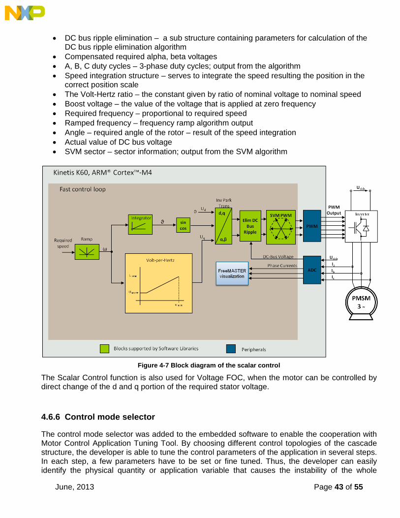
June, 2013 of 55

• DC bus ripple elimination – a sub structure containing parameters for calculation of the DC bus ripple elimination algorithm

• Compensated required alpha, beta voltages • A, B, C duty cycles – 3-phase duty cycles; output from the algorithm • Speed integration structure – serves to integrate the speed resulting the position in the

correct position scale • The Volt-Hertz ratio – the constant given by ratio of nominal voltage to nominal speed • Boost voltage – the value of the voltage that is applied at zero frequency • Required frequency – proportional to required speed • Ramped frequency – frequency ramp algorithm output • Angle – required angle of the rotor – result of the speed integration • Actual value of DC bus voltage • SVM sector – sector information; output from the SVM algorithm

Figure 4-7 Block diagram of the scalar control

The Scalar Control function is also used for Voltage FOC, when the motor can be controlled by direct change of the d and q portion of the required stator voltage.

4.6.6 Control mode selector

The control mode selector was added to the embedded software to enable the cooperation with Motor Control Application Tuning Tool. By choosing different control topologies of the cascade structure, the developer is able to tune the control parameters of the application in several steps. In each step, a few parameters have to be set or fine tuned. Thus, the developer can easily identify the physical quantity or application variable that causes the instability of the whole

June, 2013 of 55

system. The tool uses the FreeMASTER application as the platform for visualization of the measured quantities, so the developer can directly observe the response of the tuned system when the application parameters are changed. The control mode selector is defined as enumeration data type, with the following definition: typedef enum { CONTROL_MODE_SCALAR = 0, CONTROL_MODE_VOLTAGE_FOC = 1, CONTROL_MODE_CURRENT_FOC = 2, CONTROL_MODE_SPEED_FOC = 3, } MCSTRUC_CONTROL_MODE_T; The procedures to set and fine tune the application parameters aredescribed in the application notes related to MCAT tool.

4.6.7 Faults handling

The application checks the following faults: • Phase over current • Over DC bus voltage • Under DC bus voltage • MOSFET gate driver fault

The faults are automatically cleared after the fault condition is removed. Because the duration of some faults might by very short, a three-second time lag is added after the fault flag is removed and the application is switched from FAULT to STOP state. This allows the user to see the actual fault flag. The intelligent MOSFET gate drive MC33879 that is placed on the Tower MC power module latches different faults. They are described in the datasheet [7]. Faults are cleared via SPI communication protocol by software. In some situations the automatic software clearing of the MOSFT pre-driver faults does not perform well. For example, after hard over current faults, when the over current protection of the power supply acts and decreases the supply voltage level under the value of the MOSFET gate driver reliable operation. In such a case, the application has to be reset by disconnecting the supply voltage.

4.6.8 Main application motor control structure

The structures described above, together with some other application state variables and fault structures, create the uppermost layer of data structure. Its definition follows: typedef struct { MCSTRUC_FAULT_THRESHOLDS_T sFaultThresholds; /* threshold values of faults detected by software */ MCSTRUC_ADC_CURRENT_CH_OFFSET_T sADCOffset; /* Offset values for AD currents

sensing */ MCSTRUC_FOC_PMSM_T sFocPMSM; MCSTRUCT_SCALAR_CTRL_PMSM_T sScalarPMSM; MCSTRUC_POS_SPEED_EST_DQ_T sPositionEstDQ; MCSTRUC_BEMF_OBS_DQ_T sObserverDQ;

June, 2013 of 55

MCSTRUC_SPEED_T sSpeed; MCSTRUC_CONTROL_MODE_T eControl; Frac32 f32UDcBus; /* holds value of DCBus voltage scaled for DCB

faults evaluation */ UWord32 uw32FaultId; /* the number of fault that was latched. This flag

remains high also the next three seconds after the fault condition was removed*/

UWord32 uw32FaultIdPending;/* currently active fault */ UWord32 uw32CounterState; /* the counter variable used for different

application timing purposes */ UWord32 uw32TimeFullSpeedFreeWheel; UWord32 uw32TimeFaultRelease; UWord16 uw16CounterSlowLoop; UWord16 uw16DividerSlowLoop; }MCSTRUC_FOC_PMSM_OBS_DQ_T; There is only one variable gsM1_Drive within the application that has the declaration of this data type and stores all the application variables of PMSM FOC of one motor.

4.7 Interface function

The interface functions are used for the communication between the state machine and the master system. These functions are called to control and monitor the motor.

4.7.1 Switch control functions

These functions control the switch of the motor. The parameter is the boolean value determining the state of the switch: ON (true) or OFF (false). void M1_SetAppSwitch(bool bValue) To read the status of the switch, use the following function. The state of the switch is returned as the boolean value. bool M1_GetAppSwitch(void)

4.7.2 Command functions

This function commands the speed of the motor. The parameter is the Frac32 value. void M1_SetSpeed(Frac32 f32SpeedCmd) It is called from the application state machine and PORTC interrupt service. The inverse function is used to monitor the speed. It returns the Frac32 value. Frac32 M1_GetSpeed(void)

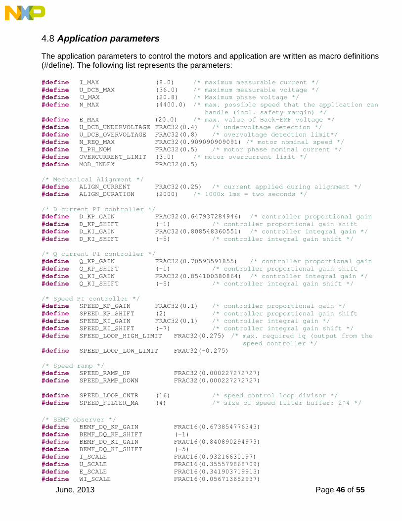
June, 2013 of 55

4.8 Application parameters

The application parameters to control the motors and application are written as macro definitions (#define). The following list represents the parameters: #define I_MAX (8.0) /* maximum measurable current */ #define U_DCB_MAX (36.0) /* maximum measurable voltage */ #define U_MAX (20.8) /* Maximum phase voltage */ #define N_MAX (4400.0) /* max. possible speed that the application can

handle (incl. safety margin) */ #define E_MAX (20.0) /* max. value of Back-EMF voltage */ #define U_DCB_UNDERVOLTAGE FRAC32(0.4) /* undervoltage detection */ #define U_DCB_OVERVOLTAGE FRAC32(0.8) /* overvoltage detection limit*/ #define N_REQ_MAX FRAC32(0.909090909091) /* motor nominal speed */ #define I_PH_NOM FRAC32(0.5) /* motor phase nominal current */ #define OVERCURRENT_LIMIT (3.0) /* motor overcurrent limit */ #define MOD_INDEX FRAC32(0.5) /* Mechanical Alignment */ #define ALIGN_CURRENT FRAC32(0.25) /* current applied during alignment */ #define ALIGN_DURATION (2000) /* 1000x 1ms = two seconds */ /* D current PI controller */ #define D_KP_GAIN FRAC32(0.647937284946) /* controller proportional gain #define D_KP_SHIFT (-1) /* controller proportional gain shift #define D_KI_GAIN FRAC32(0.808548360551) /* controller integral gain */ #define D_KI_SHIFT (-5) /* controller integral gain shift */ /* Q current PI controller */ #define Q_KP_GAIN FRAC32(0.70593591855) /* controller proportional gain #define Q_KP_SHIFT (-1) /* controller proportional gain shift #define Q_KI_GAIN FRAC32(0.854100380864) /* controller integral gain */ #define Q_KI_SHIFT (-5) /* controller integral gain shift */ /* Speed PI controller */ #define SPEED_KP_GAIN FRAC32(0.1) /* controller proportional gain */ #define SPEED_KP_SHIFT (2) /* controller proportional gain shift #define SPEED_KI_GAIN FRAC32(0.1) /* controller integral gain */ #define SPEED_KI_SHIFT (-7) /* controller integral gain shift */ #define SPEED_LOOP_HIGH_LIMIT FRAC32(0.275) /* max. required iq (output from the speed controller */ #define SPEED_LOOP_LOW_LIMIT FRAC32(-0.275) /* Speed ramp */ #define SPEED_RAMP_UP FRAC32(0.000227272727) #define SPEED_RAMP_DOWN FRAC32(0.000227272727) #define SPEED_LOOP_CNTR (16) /* speed control loop divisor */ #define SPEED_FILTER_MA (4) /* size of speed filter buffer: 2^4 */ /* BEMF observer */ #define BEMF_DQ_KP_GAIN FRAC16(0.673854776343) #define BEMF_DQ_KP_SHIFT (-1) #define BEMF_DQ_KI_GAIN FRAC16(0.840890294973) #define BEMF_DQ_KI_SHIFT (-5) #define I_SCALE FRAC16(0.93216630197) #define U_SCALE FRAC16(0.355579868709) #define E_SCALE FRAC16(0.341903719913) #define WI_SCALE FRAC16(0.056713652937)

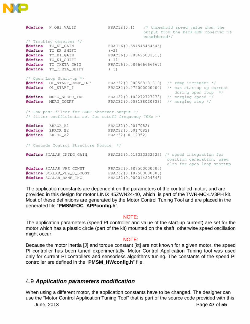
June, 2013 of 55

#define N_OBS_VALID FRAC32(0.1) /* threshold speed value when the

output from the Back-EMF observer is considered*/

/* Tracking observer */ #define TO_KP_GAIN FRAC16(0.654545454545) #define TO_KP_SHIFT (-2) #define TO_KI_GAIN FRAC16(0.789625033513) #define TO_KI_SHIFT (-11) #define TO_THETA_GAIN FRAC16(0.586666666667) #define TO_THETA_SHIFT (-5) /* Open Loop Start-up */ #define OL_START_RAMP_INC FRAC32(0.000568181818) /* ramp increment */ #define OL_START_I FRAC32(0.075000000000) /* max startup up current

during open loop */ #define MERG_SPEED_TRH FRAC32(0.102272727273) /* merging speed */ #define MERG_COEFF FRAC32(0.008138020833) /* merging step */ /* Low pass filter for BEMF observer output */ /* filter coefficients set for cutoff frequency 70Hz */ #define ERROR_B1 FRAC32(0.0017082) #define ERROR_B2 FRAC32(0.0017082) #define ERROR_A2 FRAC32(-0.12352) /* Cascade Control Structure Module */ #define SCALAR_INTEG_GAIN FRAC32(0.018333333333) /* speed integration for position generation, used

also for open loop startup #define SCALAR_VHZ_CONST FRAC32(0.687500000000) #define SCALAR_VHZ_U_BOOST FRAC32(0.187500000000) #define SCALAR_RAMP_INC FRAC32(0.000014204545) The application constants are dependent on the parameters of the controlled motor, and are provided in this design for motor LINIX 45ZWN24-40, which is part of the TWR-MC-LV3PH kit. Most of these definitions are generated by the Motor Control Tuning Tool and are placed in the generated file “PMSMFOC_APPconfig.h”.

NOTE:

The application parameters (speed PI controller and value of the start-up current) are set for the motor which has a plastic circle (part of the kit) mounted on the shaft, otherwise speed oscillation might occur.

NOTE: Because the motor inertia [J] and torque constant [kt] are not known for a given motor, the speed PI controller has been tuned experimentally. Motor Control Application Tuning tool was used only for current PI controllers and sensorless algorithms tuning. The constants of the speed PI controller are defined in the “PMSM_HWconfig.h” file.

4.9 Application parameters modification

When using a different motor, the application constants have to be changed. The designer can use the “Motor Control Application Tuning Tool” that is part of the source code provided with this

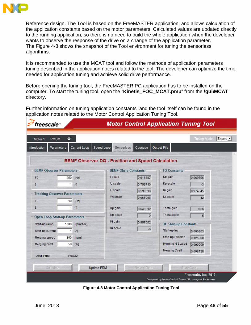
June, 2013 of 55

Reference design. The Tool is based on the FreeMASTER application, and allows calculation of the application constants based on the motor parameters. Calculated values are updated directly to the running application, so there is no need to build the whole application when the developer wants to observe the response of the drive on a change of the application parameter. The Figure 4-8 shows the snapshot of the Tool environment for tuning the sensorless algorithms. It is recommended to use the MCAT tool and follow the methods of application parameters tuning described in the application notes related to the tool. The developer can optimize the time needed for application tuning and achieve solid drive performance. Before opening the tuning tool, the FreeMASTER PC application has to be installed on the computer. To start the tuning tool, open the “Kinetis_FOC_MCAT.pmp” from the \gui\MCAT directory. Further information on tuning application constants and the tool itself can be found in the application notes related to the Motor Control Application Tuning Tool.

Figure 4-8 Motor Control Application Tuning Tool

June, 2013 of 55

4.10 Interrupts

The application requires the minimum number of interrupts due to the MCU hardware triggering the AD conversion..

4.10.1 ADC1 Interrupt

This interrupt request is triggered when the conversion of channel A of the ADC1 module is completed and has the highest priority. As the interrupt is generated, there are sampled values of physical quantities ready: in the Result Registers A of the ADC0 (DC bus voltage), Result Register B of the ADC0 (motor phase current 1) and Result Register A of the ADC1 module (motor phase current 2). The interrupt is always enabled only for one module, to avoid generating two interrupt requests at the same time, because the triggers for motor phase currents are generated in the same instance. In the beginning of the ADC1 ISR execution the Application State Machine function is called. If the application is in the Run state, the fast (current) control loop of the PMSM vector control algorithm is executed, including the position and speed estimation. As mentioned in previous chapter, the slow (speed) control loop is also calculated based on the value of the software counter that is decremented each time the fast control loop is passed. The interrupt flag is cleared by reading the result register of the ADC channel that triggered the interrupt. Therefore, the results of AD conversion are read at the beginning of each particular State Machine Function, even though the values are not used later in the program execution. The flow chart depicted in Figure 4-9 gives an overview of the program flow during the execution of the ADC interrupt service routine when the application is in Run state and Spin sub-state.

June, 2013 of 55

Figure 4-9 ADC ISR flow chart

4.10.2 PORTC interrupt

Button handling on the K60 tower board is performed in the ISR associated with the PORTC interrupt, which is generated whenever one of the buttons is pressed. At the beginning of the ISR, simple logic is executed to evaluate which button was pressed, and the interrupt flag is cleared. Because there are only two user’s buttons, control is limited. In the application, the assigned functions are RUN and STOP, and they control rotation only in one direction. Pressing the RUN button causes the speed to increase in 10% increments. Pressing the STOP button causes the speed to decrease in 10% increments.

June, 2013 of 55

For more information about the application control via the user’s buttons, see the chapter “Application control”. Using the FreeMASTER control interface allows for enhanced control and diagnostic.

4.10.3 PDB error interrupt

The PDB error ISR serves to clear the sequence error fault generated when PDB initiates the sampling of the AD converter, but the COCO flag in the particular ADCx_SC1n register of the ADC module was not cleared because the values from result registers were not read. In these cases, the PDB counter stops working and an interrupt is asserted. The PDB module is then reinitiated in the ISR. The PDB generates trigger signals with the same period as the ADC conversion complete interrupt, which is also the same as the PWM period. If the user places an interrupt in the code, this will stop the execution. The PDB will generate triggers for the next conversion, even when the program execution stops. The COCO flags are not cleared and the PDB generates a sequence error. Another reason for the unread register is that the execution of the ADC conversion complete interrupt (where the fast control loop is calculated) would extend over one period of PWM. This might happen if the user puts additional tasks into the ADC conversion complete interrupt. In addition to the generation of PDB sequence error, the more serious impact is on the quality of the control process, as one of the key assumptions is not met: the execution of control algorithms extends the sampling period. The real-time control application has to be designed in such a way that this situation never occurs. 4.10.4 Project file structure The total number of source (*.c) and header files (*.h) in the project exceeds one hundred. Therefore, only the key project files will be described in more detail, and the rest will be described in groups. The main project folder is divided into three directories:

• build – contains configuration files for the IAR compiler as well as the compiler’s output executable and object files. If the IAR Embedded Workbench for ARM is installed on your computer, double clicking the workspace file “TWRK60D100N_PMSM_SNSLESS.eww” located in the directory \build\iar\ launches the IAR IDE.

• gui – contains the FreeMASTER configuration file (“Kinetis_FOC.pmp”) and supporting files (control page in HTML format and the binary file with addresses of the variables). It also contains FreeMASTER project for Motor Control Application Tuning Tool “Kinetis_FOC_MCAT.pmp” located in the MCAT sub directory.

• src – contains the project source and header files. Its contents will be described in the following section.

Files in the root of the src folder:

main.c , main.h contain basic application initialization (enabling interrupts), subroutines accessing the MCU peripherals and interrupt service routines. In the background infinite loop, the FreeMASTER communication is performed.

state_machine.c and state_machine.h contain the application state machine structure definition and handle switching between the application states and application states transitions.

June, 2013 of 55

motor_structure.c and motor_structure.h contain the structures, definitions, and subroutines dedicated to performing the motor control algorithm (vector control algorithm, position and speed estimation algorithm, speed control loop). M1_statemachine.c and M1_statemachine.h contain the software routines that are executed when the application is in the particular state or state transition.

freemaster_cfg.h is the configuration file for the FreeMASTER interface. PMSMFOC_appconfig.h contains the definitions of constants in the application control processes (parameters of the motor and regulators, and the constants for other vector control related algorithms). The content of the file is listed in chapter 4.8 Application parameters. When the application is tailored for another motor using the Motor Control Application Tuning Tool, this file is generated by the Tool at the end of the tuning process. PMSM_HWconfig.h contains definitions of the application constants that are not generated by the MCAT tool.

Files and subdirectories in the src\mcu_Init\ folder:

\common\ and \cpu\ folders contain CPU initialization routines. \cpu\vectors.h is an important file that contains the definition of the peripherals interrupt service routines assigned to the interrupt vectors. In this file, the user can add the definition of an ISR for an additional peripheral interrupt. \drivers\ subdirectories contain generic source and header files for UART and watchdog configuration, as well as the CPU clock settings routines. \peripherals\ contains important files for static configuration of the peripherals used in the application (FlexTimers, ADC, PDB, SPI, PIT). \platforms\tower.h contains the Kinetis Tower card definitions (CPU speed and UART parameters).

Files in the src\twrk60d100\ folder:

MK60N512VMD100.h is the header file containing macro definitions of all the MCU registers and registers’ bits.

Files in the src\MC_Lib\ folder: Cortex_M4.a is a software library containing motor control, general math, and filter algorithms. Other files in the folder and subfolders are associated header files, each one for a particular function of the library.

June, 2013 of 55

Cortex_M4_ACLIB.a contains the advanced control algorithms for rotor position and speed estimation (Back-EMF observer and Tracking observer).

Other subdirectories in the src\ folder:s

\src\FreeMASTER contains all source files of the FreeMASTER application. It is not necessary to access it or change anything inside. The interface to the programmer is only via freemaster_cfg.h file. \src\MC_Lib\Common contains specific header files associated with the software libraries. \src\app_init contains the routines for MOSFET gate driver initialization, GPIO ports, and FreeMASTER initialization

4.10.5 Memory usage The following table summarizes the chip memory usage: Table 4-2 Memory Usage, Values in Bytes

Memory Total Available on the Kinetis MK60N512VMD100

Used by the Application

Program Flash (application code) 512 KB 23 854 B Data Flash (application constants) 2 046 B Data RAM (application variables) 128 KB 2 845 B

Section 5. Application set-up and operation The application can be operated via the user’s buttons on the K60 tower module, or via the FreeMASTER interface. The set-up procedure of the FreeMASTER software on the PC, as well as the application operation, is described in the User’s Manual [12].

Section 6. Results of the measurement

6.1 CPU load and the execution time

The CPU load is influenced mainly by the execution of the ADC1 ISR, in which the execution of the application state machine and calculation of the fast (current) control loop of the PMSM vector control is performed. The complete ADC1 ISR requires 2656 (state machine and fast control loop) to 2962 (with the slow control loop calculation) machine cycles. The ADC1 interrupt is generated periodically with the same frequency as the PWM reload event, when the values of the duty cycles are updated.

June, 2013 of 55

In this application, the ADC ISR is generated once per 63 µs, which corresponds to 16 kHz of the PWM frequency. At 100 MHz on the Kinetis K60 device, it consumes 42 – 47% of CPU performance.

6.2 Measured results using FreeMASTER

6.2.1 Motor startup

The motor startup is presented in Figure 6.1.. The required speed was changed from 0 to 2000 rpm. The values are captured using the FreeMASTER scope.

Figure 6-1 Motor startup from zero speed to 2000 rpm

The “Position Merge Counter” variable identifies the time section where the generated open-loop and the estimated positions are merged. When the Merge Counter reaches “1”, the application is running in the speed closed control loop. The time gap between the step change of the “Required Speed” and the instance when the “Speed Ramp” becomes non-zero represents the rotor alignment.

6.2.2 Position merging

The position merging process is shown in Figure 6.2. The chart was captured using the FreeMASTER recorder feature. For reference, an encoder position is also depicted.

June, 2013 of 55

Figure 6-2 Position Merging Process

The start of the position merging process is when the motor speed reaches 10% of the nominal speed. During the merging process, the merged position (blue) is approaching the estimated position (red). At the end of the merging process, the application enters the “Spin” sub state of the “Run” state, and the open loop and merged positions are no longer calculated. As the speed of the motor increases, the difference between the encoder position (which is used here as the reference, and provides the real physical rotor position) and the estimated position decreases.

Start of the merging process

End of the merging process

Difference is decreasing

How to Reach Us Home Page: http://www.freescale.com Web Support: www.freescale.com/support

Information contained in this document is provided solely to enable system and software implementers to use Freescale products. There are no express or implied copyright licenses granted hereunder to design or fabricate any integrated circuits based on the information in this document. Freescale reserves the right to make changes without further notice to any products herein. Freescale makes no warranty, representation, or guarantee regarding the suitability of its products for any particular purpose, nor does Freescale assume any liability arising out of the application or use of any product or circuit, and specifically disclaims any and all liability, including without limitation consequential or incidental damages. “Typical” parameters that may be provided in Freescale data sheets and/or specifications can and do vary in different applications, and actual performance may vary over time. All operating parameters, including “typicals,” must be validated for each customer application by customer’s technical experts. Freescale does not convey any license under its patent rights nor the rights of others. Freescale sells products pursuant to standard terms and conditions of sale, which can be found at the following address: freescale.com/SalesTermsandConditions. Freescale, and the Freescale logo, are trademarks of Freescale Semiconductor, Inc., Reg. U.S. Pat. & Tm. Off. All other product or service names are the property of their respective owners. . © Freescale Semiconductor, Inc. 2013. All rights reserved. .

http://www.freescale.com/�

http://www.freescale.com/support�

http://www.freescale.com/SalesTermsandConditions�

pmsm sensorless vector control on kinetis€¢ application speed ranges from 0% to 100% of nominal...

Documents