pm doc

POSTMARC A Windows Postprocessor for CMARC and Pmarc

Version 7

Program and Documentation Copyright David Pinella 2013All Rights Reserved

1. SYSTEM REQUIREMENTS AND INSTALLATION 1Environment 1Installation 1

2. DATA FILES 3Input file types 3

3. VIEW MANAGEMENT 5Types of depiction 5Rotating the model with function keys 5Rotating the model with the mouse 6LMP View Logic 6Orthogonal views 6Setting a viewpoint 6Default perspective viewpoint 7Stored views 7Magnification 7Zooming 8Panning 8Solid colors 8Patch selection 8Wakes 9Saving wakes 10Displaying the wake separation line 10Selecting and displaying panels with tilted vectors 11

4. DISPLAYS OF PRESSURE AND VELOCITY 13Selection of units 13Contour lines 15Screen XY Plots 16Differencing 17Mapping Cp to imported meshes 17

5. SURFACE FLOW DIRECTION AND STREAMLINES 19Local velocity vectors 19Displaying on-body streamlines 20Generating streamlines in POSTMARC 21Selecting streamline locations 21Calculating on-body streamlines 22Forcing laminar transition 22Generating boundary layer data for the complete model 23Displaying boundary layer characteristics 23Boundary Layer Separation Criterion 23XY plotting of on-body streamlines 24Preventing premature separation 24

6. OFF-BODY FLOW 27Off-body streamlines from CMARC 27Calculation of off-body streamlines by POSTMARC 27

Single streamlines 28Multiple streamlines 28Interactive selection of streamline locations 29XY plotting of off-body streamlines 29Rectangular and cylindrical velocity scans 30Scan volumes computed in POSTMARC 30Defining a rectangular scan volume 31Saving scan volume data 31Single Point Calculation 31Displaying rectangular velocity scans 32Contouring scan planes 32Cylindrical scan volumes defined in POSTMARC 33Cylindrical scan volume display 34Scans from imported point lists 34

7. INFORMATION ABOUT INDIVIDUAL PANELS 35Geometry and aerodynamic data (individual panels) 35Panel XY plots 35Integrated XY plots 36

8. INTEGRATED FORCES AND MOMENTS 37Patch and air data selection 37Information for stress analysis 38Stability derivatives and lift curve slope using CMARC 40Neutral point 41Elevator angle to trim 41Stability analysis with DWT 41Inertial calculation 42Inertia of discrete components 42Inertia of the model surface 43

9. OUTPUT OPTIONS 45Hard copy 45Saving to the clipboard 45POV-Ray 45VRML 46DXF 46

1

1. System requirements and installation

Environment

POSTMARC runs under Windows, using the OpenGL graphics platform. Mostgraphics processors will handle OpenGL without difficulty, but if problems (suchas incorrect hidden-surface and hidden-line elimination) are encountered witholder processors it may be necessary to disable some graphics accelerations. Todo this, go to My Computer > Control Panel > Display > Settings > Advanced >Troubleshoot and move the slider left to the second detent.

To suppress the legal agreement dialog that appears at the start of a program run,set the environment variable PSW_AGREE_YES by going to the Windows ControlPanel, the System icon, the Advanced tab, and the Environment Variables button.

Installation

Normally, installation is handled automatically by the distributed installationprogram and the principal executable files are automatically added to theWindows Start menu. POSTMARC should be installed in the same folder asCMARC and/or DWT. The folder should also contain a copy of CMARC.DIM.

Once POSTMARC has been installed in the desired folder, you can place an iconon the desktop by locating the POSTMARC executable (POSTMARC.EXE) with theWindows Explorer, right-clicking to create a shortcut, and dragging the shortcuticon onto the desktop.

3

2. Data files

Input file types

POSTMARC reads both binary (.BIN) and formatted ASCII (.FMT) plot filesproduced by Pmarc or CMARC. Both types of file contain the same information,but binary files take up less disk space and load more quickly. On the otherhand, ASCII files are more easily portable between operating systems, and it issimpler to write programs to recover information from them. So far as informationmining is concerned, however, most of the information in the .BIN/.FMT file canalso be retrieved from the ASCII .OUT file.

Which type of output file CMARC produces is controlled by the LPLTYP flag in theinput file. The flag may be overridden from the command line in the DOS versionof CMARC; otherwise, it must be edited in the .IN file. For binary output, which isthe default, LPLTYP should be zero.

POSTMARC automatically identifies the type of the input file, the .BIN file havingprecedence in cases where both a .BIN and a .FMT file have the same name. All.BIN and .FMT files in the default directory are displayed in the file selectionwindow.

POSTMARC also uses or creates other files, with extensions such as .PM, .ONB,.OFB, .RVS, .CVS, .PMX, and so on. The .PM file, which is generated by CMARC,is the basic source of data used for post-computing streamlines, boundary-layercharacteristics, velocity scans, and so on. None of these files is created by Pmarc.

None of POSTMARC's input files, except CMARC.DIM, is intended to be modifiedby the user.

5

3. View management

Types of depiction

The model and its wake(s) may be displayed as a transparent wireframe or asopaque 3D surfaces with hidden lines and surfaces eliminated. To select theopaque 3D display, which is the most generally useful one, select View > HiddenLine.

To return to either of the basic depiction types after mapping colors or otherinformation onto the model surface, hit <Esc>.

Setting the model's position

A model initially appears in top view. Several methods are available for viewingthe model from different angles. They are 1) rotating the model in roll, pitch, andyaw, with the function keys or with the mouse; 2) directly setting an orthogonalview or a default perspective view; and 3) setting the direction cosines of an eyeposition with respect to the model coordinate system.

The model is not automatically kept in the center of the screen when it is rotated.To move it, hold down the right mouse button and drag the model.

Rotating the model with function keys

The model can be rotated with the function keys F5 through F10, which controlrotation about the X, Y, and Z axes of the model (F5, F6, F7) and the screen (F8,F9, F10) respectively. Hidden lines may be removed to resolve ambiguity. The<Shift> key reverses the direction of rotation. Positive (unshifted) rotationfollows the right-hand rule; that is, when the right hand is held with the thumbpointing in a positive direction along an axis, rotation about that axis is positivein the direction the fingers curl.

To return the model to its initial position, click on the "reset" button.

6

Rotating the model with the mouse

Two sets of conventions are provided for rotating the model with the mouse. Oneset, selectable by View > LMP View Logic, is similar to those used by LOFTSMAN;the other is similar to those used by the original version of POSTMARC, andrequires holding F3 (while moving the mouse) to perform rotations, F2 to zoom,and F1 to move the model.

LMP View Logic

The LOFTSMAN viewing system is based on the idea of a transparent globe withthe model at its center. The observer is sprawled on the surface of this globe,head north, peering inward. Mouse movement controls the latitude and longitudeof the observer.

In this scheme, the model is always upright; that is, its Z axis passes though thenorth pole of the globe. To rotate the entire view, move the mouse on the left-rightaxis while depressing both buttons; this has the effect of rotating the observeraround his own eye(s).

Orthogonal views

As a shortcut to the three standard orthogonal views, the X, Y, and Z keys can beused. The lowercase letters produce views looking in a negative direction, ortoward the origin, along the corresponding axes (ie rear, starboard, and topviews); uppercase produce views looking in a positive direction or away from theorigin (ie front, port, and bottom views).

Setting a viewpoint

The button with the eye icon is the "viewpoint" control. It is used to set the viewdirection. The dialog box requests three values. These are not angles, but ratherx,y,z coordinates of the point in space, with respect to the global origin, at whichthe viewer's eye is located. For example, eye location [1 0 0] will be lookingforward (toward the origin) along the X axis. Location [-1 0 0] looks aft along the X

7

axis toward the origin. Positive Z values indicate an eye position above the planeof the model. Positive Y values indicate a position to the model's right or starboardside. Coordinates may be fractional, but their absolute size is not important;rather, their relative sizes determine the angle from which the model is viewed.Thus, [10 5 4] produces the same view as [1.0 0.5 0.4]. Perspective convergencehas not been implemented, and so distance from the origin is irrelevant.

While viewpoint is not a very intuitive method of positioning an object, it doeshave the advantage of providing a numerical equivalent of a view so that it can beduplicated at a later time or in different programs that provide this method.

Default perspective viewpoint

To obtain a default perspective view, hit p or Shift-p.

Stored views

In addition to the three orthogonal views and the default perspective view,POSTMARC will store up to 20 "key views" which are accessible using the digitand shifted-digit keys.

To store a view, position the model, then select

View > Key Views

and click the V button next to an unused digit. Henceforth (or until you storeanother view in the same location) typing that digit will produce that view.

Magnification The button whose icon resembles a magnifying glass controls magnification.Normally the default magnification (1.0) scales the model to fit within the screen.A factor larger than 1.0 enlarges the model and one smaller than 1.0 shrinks it.Negative numbers are meaningless and are not accepted.

8

Zooming

To zoom, first click the zoom button, then move the mouse to one corner of thedesired viewing area and, with the left mouse button depressed, drag a boxaround the part of the model at which a closer look is desired.

To unzoom, click on the "reset" button.

Use the magnification button, rather than the reset button, to partially reduce themagnification of a zoomed view.

An alternative method of controlling magnification and zooming is provided by the<F2> key when LMP View Logic is not being used. Vertical motion of the mousewith the <F2> key held down makes the model get larger and smaller.

The scroll wheel on the mouse may also be used to control zooming.

Panning

To move the model to a different location, drag it while pressing the right mousebutton.

Solid colors

When hidden-line removal is used, model surfaces may be colored. Select View >Colors from the menu.

You can set different colors for the outer and inner surfaces of the model --indispensable for checking patch orientation -- and for the "tops" and "bottoms" ofwakes. On the model, positive corresponds to the outer surface. On wakes, thedistinction between top and bottom is meaningless, but surface types should beconsistent throughout any given wake sheet.

Patch selection

Any patch or group of patches may be selected or deselected for display. Click onView > Patch Selection.

9

To look at the inside of a duct, for example, the outer portion of the model can be

removed, provided that it has been defined as a separate patch. Patch selection isalso important in obtaining integrated force and moment data for portions of amodel. Only the portions of the model that are visible on the screen are includedin the summation.

Wakes

To display one or all wakes, select

Display > Display wake(s)

Like the model surface, wakes are displayed as a wireframe or with hidden linesremoved, depending on the selection in the View menu.

10

To animate the wake(s), select

Display > Animate wake

or click on the wake icon in the toolbar. Wakes are numbered in the order inwhich they appear in the input file. Highlight the wakes you want to see. Wakeanimation continues to cycle until you hit <Esc>.

Saving wakes

It some cases, such as analyses of multi-element airfoils, it is quicker and simplerto have CMARC generate the wakes (INITIAL=0) than for the user to define them.This is still a long process, however, requiring about 20 time steps, and it wouldhave to be repeated for each run of CMARC.

Once a wake has been defined, POSTMARC can file it in the proper format forinclusion in a CMARC input deck. When a developed wake has been edited intoan .IN file, additional cases can usually be run without any time stepping at all solong as the angle of attack is not too far different from the original one.

Select

Calculations > Write Wakes

Normally, the wake shape at the final time step should be used, but only afterchecking that it is well formed.

By checking Write separation line only at the bottom of the form, you can makePOSTMARC write into a .WSL file the node coordinates for a wake separation line.This in turn can be read by LOFTSMAN to produce a wake for geometriesinvolving fuselage sides that are parallel or diverge behind the wing. For thispurpose it is not necessary to fully develop a wake in CMARC; a single step issufficient.

Displaying the wake separation line

When a CMARC input file includes a wake separation line and an analysis hasbeen performed that includes wakes, the wake separation line can be displayed bychecking View > Wake Separation Line. The WSL display alternates colors panel bypanel to help you verify that it is not jumping panels.

11

Selecting and displaying panels with tilted vectors

Tilting surface normal vectors is aconvenient and accurate method ofsimulating control surface deflectionsup to angles of about 15 degrees.Panels with tilted vectors are identifiedon the &BINP11A line of the CMARCinput file; see the CMARCdocumentation for a fuller discussionof this procedure.

Panels with tilted normal vectors canbe both selected and displayed inPOSTMARC.

To display panels, select View > TiltPanels > Manage/Write. Check View TiltPanels and supply the requestedinformation for whichever source you

have chosen.

Three sources are possible. First, you can define a panel or group of panels byentering data in the area captioned Manual Input. The items here are the same asthose in line &BINP11A of the CMARC input file; groups of panels are defined bytheir first and last rows and columns. Check View Tilt Panels and Manual Input tohighlight selected panels. Highlighted panels are visible only in the hidden linemode.

Second, you can display all or some of the panels defined in the CMARC input file.Click on Load .in. If the name of the appropriate input file is different from that ofthe file currently loaded, you must enter it before selecting Load .in. The list box ispopulated with all of the tilted panels defined in the input file. You can select fromamong them (or select all of them), and then click on View from Cmarc/DWT .

Finally, you can manually select panels and have POSTMARC write your&BINP11A line for you. Select View > Display Tilt Panels > Pick panels and selectpanels by placing the crosshair over them and doubleclicking the left mousebutton. Hit <Enter> to finish the process, or <Esc> to abort it. Then return to theDisplay/Create Tilt Panels dialog, select Cursor picked and Create CMARC cards,and provide a file name. This file will contain a &BINP11A line ready to edit intothe CMARC input file.

13

4. Displays of pressure and velocity

Selection of units

The basic inviscid analysis is independent of Reynolds number. Boundary-layeranalyses, on the other hand, require that you specify fluid density and viscosity.To set these values, select

File > Units

Then select the appropriate fluid and, in the case of air, enter the altitude. Thedensity and viscosity are displayed and become the default values.

Contour plots

The following potential-flow properties can be mapped in colors on the model:

Pressure coefficientGauge pressureVelocity magnitudeMach number

In addition, after a boundary layer analysis has been performed by “coating” themodel with streamlines, the following properties may also be mapped:

Boundary layer thicknessDisplacement thicknessShape factorSkin friction coefficientLaminar transition

In addition, a two-color plot is available to identify areas where BL data have notbeen found. These may be areas of separated flow or areas where streamlinesfailed to be calculated for some technical reason such as a too-sharp bendbetween two panels.

Thicknesses are given in geometry units. Pressure and velocity coefficients areeasy to understand, but in order for Mach number to have comprehensibledimensions, the values of VSOUND and VINF in the CMARC input file should

14

reflect their proper ratio. Thus, if the dimensions of a model are in inches and theflight speed of the model for a given analysis is actually going to be 4,000 inchesper second, but VINF is set at 1.0, then VSOUND should be set at 13,392/4000,or 3.348. In other words, VSOUND should be set to the speed of sound ingeometry units multiplied by VINF and then divided by the actual flight speed ingeometry units.

To set contouring parameters, click on the Display Options button or select Display> Options from the menu.

The dialog presents a number of options:

Fringe contours: Raw data from CMARC provide a single pressure for each panel.When fringe contours are turned on, pressures are interpolated across panels,producing smooth transitions that more closely approximate the actualvariations of pressure distribution. Fringe contours are on by default.

Include Panel boundaries: Panel boundaries may be indicated or omitted. Sincethey help to convey the shape of the model, they are on by default.

Automatic levels: The range of values represented by the color spectrum may beadjusted by the user, or may be selected by POSTMARC.

The advantage of having the program set the range is that you can switch amongdifferent types of output, such as pressures and velocities, whose values are ofdifferent magnitudes, without having to manually readjust the color range aftereach change.

15

The disadvantage is that many analyses that are otherwise valid include a fewunrealistic values which may distort the range, compressing the useful band inan undesirable way. To protect against these outliers, POSTMARC can omit somevalues at the extremes. The size of the clipped area, as a percentage of the totalnumber of values, can be set by the user (% Clipping).

When levels are set automatically, the limits can be rounded to convenient values.The effect is to enlarge the displayed range somewhat, without going to theextremes that outliers may cause. Check Smooth Min/Max.

Levels may be set manually to emphasize particular information. For example, avery narrow range of Cp values, such as -0.01 to +0.01, could be used to locateareas on a fuselage where pressure is close to static. The realistic range of Cpvalues for aircraft is from -5.0 to +1.0, but a narrower range, for example from -0.4 to +0.4, is usually more informative.

Symmetry: The model may be mirrored about the zero plane in any axis. Formodels that are symmetrical about the vertical plane, as aircraft normally are,the plane of reflection is the XZ plane. The default is None.

Number of colors: Larger numbers provide a smoother appearance. The largestpermissible entry is 255.

% line offset: In order to ensure that lines representing contours, onbodystreamlines, or surface force vectors are visible, they are drawn slightly abovethe model surface. If lines appear dashed, increase the value of the offset. Thedefault is 0.01. This value also applies to highlighting, for instance when youclick on panels to select them.

When you have made all your selections, click on the plot icon (rainbow oval) orselect Display > Contour Solid to display the spectrum plot.

To return to the uncontoured hidden-line depiction of the model, hit <Esc>.

Contour lines

Pressure, velocity and Mach maps can also be displayed as contour lines ratherthan filled and blended colors. Click the Lines Contour button or select Display >Contour Lines. Relatively few colors should be used in order to avoid proliferation oflines of practically the same color and excessive crowding of lines in areas of rapidpressure change.

16

Screen XY Plots

After a contour map has been drawn, an XY plot of the variation in pressure,velocity or Mach number along any cross section may be obtained. The verticalrange of the graph will be the same as the one selected for the spectrum plotunless you instruct POSTMARC to scale the plot automatically.

To define a section, display any view of the model and click on the cross-sectionbutton or select Display > Screen XY Plot. Then move the crosshair cursor to thepoint at which the section is to begin. Press the left mouse button, drag a line tothe other end of the desired section, and release the mouse button. Coordinates ofthe cursor are continuously displayed at the bottom of the work area.

"Top" and/or "bottom" surface contours may be selected; these are in fact thesurfaces nearer to and farther from the viewer. If only one line appears, thereason is most likely that both contours are identical, and one has overwritten theother.

Another option is a line representing the sum or difference of the "top" and the"bottom." When the surface in question is a wing, this line gives an approximaterepresentation of the chordwise lift distribution. It should be kept in mind,however, that pressures act normal to the surface whereas lift is normal to thewind axis; and so the Y values represented by the "sum" line are not exact unlessboth top and bottom surfaces at a given station are horizontal or early so.

The raw data on which XY plots are based may be saved in tabular form. CheckSave to XY.

17

POSTMARC provides the option of saving and displaying XY data in Excel. If youwant to use Excel for this purpose, check that option in the View submenu. Youmay optionally open a new or an existing Excel file or close a file currently in use.If you do not select any of these items, POSTMARC automatically opens a newinstance of Excel for XY plotting.

Differencing

POSTMARC will map the differences between two models in any plottableparameter. The models must be similarly paneled, but can differ in dimensionsand/or in flight conditions. They can even differ in shape, so long as the patchcount, and the number of rows and columns within each patch, are the same.

To load a second file for differencing, select

File > Open secondary

After you make a selection, all commands related to pressure, velocity, and Machnumber (including pressure distribution graphs and integrated forces andmoments) relate to the two files together.

The default operation is second file minus first file. You can select first-minus-second or even first-plus-second by clicking on File > Two File Operator.

To turn off differencing, select File > Two File Operator and check None.

Mapping Cp to imported meshes

Loads may be mapped to either nodes or element centroids of non-CMARC FEAmeshes. In either case, the points for which loads are desired must be supplied inthe form of a simple ASCII list of coordinate triplets.

Select Derived Data > Map Results to FEM. Select a time state and a tolerance;POSTMARC will flag, for your information, all points for which the given pointdiffers from the corresponding location on the surface of CMARC model surface bymore than the tolerance. Provide the name of the input file containing the FEMpoint list and click on Map Cp to FEM.

POSTMARC produces a file in which the input coordinate list is duplicated, withthe assigned pressure added alongside each point’s coordinates.

19

5. Surface flow direction and streamlines

Local velocity vectors

Direction and velocity of local surface flow may be displayed as arrows originatingfrom the centroid of each panel.

The direction of the arrow indicates the orientation of the local flow. The color ofthe arrow indicates the flow speed, pressure or Mach number. Arrow lengthindicates nothing, but can be adjusted in the Display > Options dialog under VectorDisplay.

To enhance the visibility of arrows, the model surface is made white.

20

Displaying on-body streamlines

On-body streamlines originate from the centroids of specified panels and arecomputed upstream or and downstream until the end of the body or a stagnationpoint is reached or turbulent separation is predicted. In real life, separatedturbulent flow may in some cases reattach farther downstream, but turbulentreattachment will not occur in the numerical simulation.

The colors of streamlines may encode a number of boundary layer conditions inaddition to the usual pressure and velocity. These are:

B.L. thicknessDisplacement thicknessShape factorLocal skin friction coefficientStreamline state and thickness

When Streamline state is selected, the predicted point of laminar transition isindicated by a black dot.

1) Select a display option2) Choose a range of streamlines eg 1,53) Choose ALL streamlines eg *

21

For more prominent display of streamlines on printed output or on high-resolution displays, the width of the streamline image in pixels can be adjusted.

Generating streamlines in POSTMARC

The CMARC input file provides for definition of on-body streamlines with specifiedflow conditions (Reynolds number and kinematic viscosity). It is inconvenient topreselect streamlines, however, both because it is cumbersome to obtain ahead oftime the ID numbers of panels through which the desired streamlines will pass,and because the analysis must be repeated for each new set of boundary-layerconditions.

POSTMARC, however, can compute streamlines for any or all panels, and for anyboundary layer parameters, after a single CMARC run. The information used byPOSTMARC is stored by CMARC in a file with the extension .PM.

A binary .PM file is automatically created by CMARC. CMARC can be made towrite an ASCII .PM file instead, for instance if portability between UNIX andWindows systems is desired, by checking Write Postmarc data in ASCII format orby adding -pa to the DOS command line. POSTMARC automatically determinesthe type of .PM files when it reads them.

Selecting streamline locations

From the menu select

Calculations > Create On Body > Pick Panel Passing

Place the cursor over each panel through which you want a streamline to passand double-click the left mouse button. The panel is highlighted. When you havefinished, hit <Enter>.

Since onbody streamlines are calculated both forward and backward from thepoint you select, a single panel defines a streamline that may run the entirelength of the model. If you wish to cover the entire body with streamlines, do notpick panels; go directly to Manage/Calculate.

22

Calculating on-body streamlines

When one or more streamlines have been identified, select

Calculations > Create On Body > Manage/calculate

A dialog box appears. If you have picked panels manually, they are listed; some orall of these may be chosen for processing. If you want to ensure that at least onestreamline passes through every panel on the model, do not select any cursor-picked panels, but check Cross All Panels instead.

Processing of boundary layer data is optional. If you want a full boundary layeranalysis, you must check Include Boundary Layer Calculation. If you do notsupply values for Reynolds number and kinematic viscosity, POSTMARC looks inthe .PM file for the values, if any, that were specified in the CMARC input file. Ifthere are no values in the input file, or NBLIT is not set to 1, POSTMARC willwarn that the values it found in the .PM file are unreasonable. In this case, enternew values in the dialog box before proceeding.

Calculated streamlines are appended to a file with the same name as the .PM file(which is the same as the name of the input file) but having an .ONB extension. Itis not possible to weed streamlines selectively out of this file. It is possible,however, to delete the file altogether with the button marked Delete Streamlines.

Forcing laminar transition

Laminar transition may be forced at a desired location. Select

View > BL Trip Geometry > Pick Points

Doubleclick at two or more locations to define the trip line. Hit <Enter> toterminate a line or <Esc> to abort. When you terminate a line, the View/CreateBL Transition Geometry dialog appears. (This dialog may also be reached via View> BL Trip Geometry > Manage/Write.) It allows you to select line segments to display,and also to create BINP13 and BINP15 cards for editing into an input file. Tomake the trip line(s) visible, check View BL Transition Geometry.

To create separate trip lines in different locations, repeat the process.

Trips can be created for temporary use or made a permanent part of the input file.To incorporate a trip line in the input file, first define the lines, then click onCreate Cmarc Cards. A text file will be created containing BINP13 and BINP15lines ready to edit into the CMARC input file. Streamlines generated in CMARCwill be affected by these trips unless you change the value of NBLTRIPSEGS tozero. Streamlines subsequently generated in POSTMARC, however, will be affected

23

only if you load and select the trip lines in the View > BL Trip Geometry >Manage/Write dialog.

Generating boundary layer data for the complete model

If you select Cross All Panels, POSTMARC will automatically generate a streamlineto cross every panel in the model. Nearly all streamlines will cross more than onepanel, and many panels will be crossed by more than one streamline. Theresulting information density is equal to that in the basic pressure/velocityanalysis.

Values derived from this operation can be integrated to obtain friction drag for theentire model or for selected patches, and to provide spectrum plots of anyboundary layer parameter.

Displaying boundary layer characteristics

Boundary layer characteristics may be mapped over the entire model in the formof a spectrum plot by selecting the appropriate button in the Solid Contour dialog.Automatic levels may be used for all parameters.

Boundary layer separation criterion

In developing the boundary layer along a streamline, a numerical parameter isused to detect turbulent separation. The default value of this parameter is 0.02.CMARC, DWT and POSTMARC all allow changing this parameter.

The separation parameter is of limited generality. A value that results in arealistic prediction of separation on a wing does not give a realistic prediction fora body of revolution. It is not possible, therefore, for a single value to provide asatisfactory prediction of separation for a complete aircraft model. For a specificisolated component such as a wing or an airship hull, however, it is possible tocontrol the onset and propagation of separation with the separation parameter.For a wing of typical planform and airfoil section, a value in the vicinity of 0.07yields a plausible-looking separation pattern.

In order to select the separation criterion, it is necessary to know the expectedseparation behavior. When a value has been found that produces a reasonable-looking separation pattern, test conditions can be varied to investigate, for

24

example, the progression of the stall with increasing alpha, or the value can beapplied to a nonlinear (viscous) analysis. The results can yield useful trendinformation, but should not be relied upon for absolute values of BL-influencedparameters such as friction drag.

XY plotting of on-body streamlines

To inspect the variation of any parameter along a streamline as a function ofchordwise location, select XY Plot in the Display > On Body Streamlines dialog. Onlyone streamline can be XY-plotted at a time. Enter a streamline number in eitherthe from .bin file (that is, calculated in CMARC) or the from .onb file (calculated inPOSTMARC) field, depending on how the streamline was calculated in the firstplace.

The order in which streamlines are generated when coating the body is essentiallyrandom, and so it is not possible to know or guess the ordinal number of adesired streamline in a complete coverage. If you do not know the number of thestreamline you want to XY plot, two courses are available. One possibility is toerase the .ONB file (in the Calculations > Create On Body > Manage/calculate dialog)or to temporarily rename it, and then generate a single streamline passingthrough the panel of interest and inspect it.

Alternatively, you can select a single streamline, generate it, and note the numberof streamlines that existed previously, which is reported when the calculationends. The new streamline will have been added to the end of the currently existing.ONB file, and its number will be one greater than the previous total.


Preventing premature separation

A rapid rise in pressure, such as may occur at the base of a windshield or aspinner, will sometimes produce a "turbulent separation" signal. When suchseparation occurs in the simulation, the flow does not reattach downstream as itwould in real life. If you see large areas of magenta extending to the tail in the Cfdisplay (indicating zero Cf), this is the likely reason.

To prevent this problem, you can recontour the area where the spike occurs tosmooth the transition from one surface slope to another. One or more off-bodystreamlines can be tested to suggest the shape the air "prefers." The effect ofrecontouring is not completely unrealistic; it simulates the effect of a pool of dead

25

or rotating air, which does, in fact, occur at the base of a windshield and in othersimilar situations.

If the nonlinear option is used to generate streamlines in CMARC/DWT, thenstreamlines can be made to "jump" over panels where a temporary separationoccurs. See the CMARC/DWT manual for an explanation of panel jumps.

27

6. Off-body flow

Off-body streamlines from CMARC

The paths of arbitrarily selected off-body streamlines computed in CMARC can bedisplayed. Off-body streamlines originate from points in the space surroundingthe model, and propagate upstream and downstream.

The coordinates of the point of origin and the limits and step size for propagationmust have been included in the CMARC input file.

Off-body streamlines are color-coded to indicate local flow conditions. Theparameters that can be coded are pressure coefficient, velocity magnitude, andMach number.

Calculation of off-body streamlines by POSTMARC

As in the CMARC input file, streamlines are defined by a point of origin, upstreamand downstream distances, and the interval between points along the streamline.

Select

Calculations > Create Off-Body

A dialog box appears. The topmost items, up- and downstream distance (SU andSD), interval (DS), and the intersection-check toggle, are common to all off-body

28

streamlines. The intersection-checking toggle selects or deselects a routine thatverifies at each station whether the streamline has penetrated the surface of themodel. This operation somewhat slows down the calculation, and it can beomitted for streamlines sufficiently far from the body to be in no danger ofcolliding with it.

There are two basic choices: single and multiple streamlines.

Single streamlines

In the portion of the dialog headed Single Streamlines, enter three coordinatesdefining a point outside the model through which the streamline passes, and thenclick Calculate Single Streamline. When the streamline has been computed, clickOK. The streamline may now be displayed by selecting Display > Off BodyStreamlines or by pressing the Off-body Streamlines button on the toolbar.

Multiple streamlines

Multiple streamlines are defined by means of a rectangular grid of points.

The grid is defined by three points representing the corners of a parallelogramwhose orientation in space is arbitrary. The first point defined, [X0 Y0 Z0], can bethought of as the origin of the parallelogram. The order of entry of the tworemaining points is unconstrained, but most usually the second point, [X1 Y1Z1], defines the horizontal extent of the parallelogram and the third point itsvertical extent.

The parallelogram may collapse to a line when a set of coplanar streamlines isdesired.

Below the second and third columns are fields labeled # Points. These representthe number of equally spaced points along the corresponding edge of theparallelogram. The total number of streamlines computed will be the product ofthese two numbers.

When the grid has been defined, click Calculate Multiple Streamlines. As withsingle streamlines, click Done when the calculation is complete.

29

Interactive selection of streamline locations

A convenient method of defining limited numbers of offbody streamlines isinteractively, using the "wand" (so called because it mimics a wind tunnel smokewand). This method requires first setting the X-axis station of a grid surfacenormal to the free-stream vector, and defining upstream and downstreamdistances and a step size, as in the other methods.

Select

Calculations > Create Off Body > Wand

Specify the wand plane location, the upstream and downstream lengths of thestreamlines, and the interval size. Place the cursor on the grid and double-clickthe left mouse button. The streamline passing through that point is immediatelycalculated and displayed.

When you have finished calculating streamlines by the "wand" method, hit<Enter>. POSTMARC gives you an opportunity to save the streamlines.

You can rotate the model and perform various other operations while the "wand"is active.

XY plotting of off-body streamlines

To inspect the variation of Cp, velocity magnitude or Mach number along an off-body streamline, select XY Plot in the Display > On Body Streamlines dialog. Onlyone streamline can be XY-plotted at a time. Enter a streamline number in eitherthe from .bin file (that is, calculated in CMARC) or the from .ofb file (calculated inPOSTMARC) field, depending on how the streamline was calculated in the firstplace.

Streamlines are numbered in the order in which they were defined. If you do notknow the number of the streamline you want to XY plot, two courses areavailable. One possibility is to erase the .OFB file (in the Calculations > Create OffBody > Manage/calculate dialog) or to temporarily rename it, and then generate asingle streamline passing through the panel of interest and inspect it.

Alternatively, you can define a single streamline, generate it, and note the numberof streamlines that existed previously, which is reported when the calculationends. The new streamline will have been added to the end of the currently existing.OFB file, and its number will be one greater than the previous total.

30


Rectangular and cylindrical velocity scans

Flow speed, direction and pressure may be displayed at three-dimensional grids ofoff-body points defined either in the CMARC input file or in POSTMARC. Gridsmay take the general form of a cylinder or a parallel-sided hexahedron (that is, asheared, or un-sheared, rectangular prism).

Velocity scans are defined by means of either a hexahedral volume throughoutwhich points are arranged in parallel arrays, or a cylindrical volume in whichpoint planes are arrayed radially. For the sake of clarity, and because this is thenomenclature used in Pmarc-12, hexahedral scan volumes will be referred to as"rectangular," even though their sides are not necessarily orthogonal.

To display scan volumes, click on the appropriate icon in the toolbar. Theparameter being mapped to color and the color range are set, as usual, throughthe Display Options form (rainbow icon).

Scan volume data are always drawn from the last time step in the original CMARCrun.

Scan volumes computed in POSTMARC

Velocity scans can be performed by POSTMARC using data saved in the .PM file.

As in CMARC, definition of a scan volume requires specifying the parameters ofthe "box" or cylinder to be scanned. In the case of the rectangular scan, these arefour corners of the volume. In the cylindrical scan, they are the axial start andend of the cylindrical volume, its inner and outer radius, the number of radialrows of points and the number of points in each row. Select

Calculations > Create Velocity Scans

Three further menu choices are offered: Rectangular, Cylindrical, and File.

31

Defining a rectangular scan volume

In the dialog box, enter the coordinates of one corner and three additional pointsrepresenting the extents of the box in length, width and height. The sides of thebox need not be parallel to the orthogonal planes.

The following example defines a scan volume around the wing of the POMARCsample file. The box is swept to contain the wing.

Origin: X = 125, Y = 18, Z = 20Point 1: X = 230, Y = 18, Z = 20Point 2: X = 235, Y = 120, Z = 20Point 3: X = 125, Y = 18, Z = -20

In the fields captioned # Points, specify the number of points to be distributedevenly along each axis of the scan volume.

Check Intersection calculation to ensure that POSTMARC does not attempt tocalculate values for points located inside the model. This is not necessary if theentire scan volume is clearly located outside the model.

After defining a scan volume, press Calculate Scans.

Saving scan volume data

If you check Save to .dat, the current scan volume data are written to a text file.

All scan volumes associated with a particular model are saved consecutively inthe same file, which has a "DAT" extension. It is up to the user to rememberwhich is which, or to find out by displaying them. The order of items for eachpoint is the same as in the OUT file. It begins with three columns of array indices.Next come three columns of Cartesian coordinates, three columns of directionvector components, and, finally, three columns containing, respectively, velocitymagnitude as a coefficient of VINF, pressure coefficient, and Mach number.

Single Point Calculation

Scan volume data can be obtained for single points by selecting

Calculations > Create Velocity Scans > Rectangular

32

Enter the coordinates of the point in the lower frame and click Calculate SinglePoint.

Displaying rectangular velocity scans

Velocity scans are displayed as arrowsoriented with the local flow direction. Thecolor of each arrow indicates the magnitudeof one of the plottable parameters, namelyCp, Velocity magnitude, or Mach number. Thelength of the arrow has no meaning.

To contour the model surface while displayinga velocity scan, click Contours - Solid.

Optionally, the velocity of the free stream canbe subtracted from each local velocity, so thatthe orientation of arrows represents thevelocity increment created by the model. Theimage at left shows induced circulationaround the wings of a Sopwith Camel.

Contouring scan planes

POSTMARC will create and display contour maps of pressure, velocity, or Machnumber over one or more planes within a rectangular scan volume. Only planescontaining points can be contoured.

After computing a scan volume, press the Contour velocity scans (slices) icon onthe toolbar or select Display > Contour Velocity Scans.

Select the scan type and the parameter to be displayed. Select the scan to displayby entering its sequential number in the DAT file. Click Load # Pts to bring thenumber of points in each scan plane into the form.

You may select one, several, or all planes along any axis. To contour the model inthe same display, click Contours - Solid and select the parameter to be contoured.

33

Click OK to display the contours.

Cylindrical scan volumes defined in POSTMARC

The cylinder geometry is described as for CMARC input, and the data input formuses the same nomenclature.

Select

Calculations > Create Velocity Scans > Cylindrical

First, define the origin of the central axis ([X0 Y0 Z0]). This will normally be on thefront surface of the cylinder. Next, define the other end of the central axis ([X1 Y1Z1]).

Third, define a point ([X2 Y2 Z2]), on an arbitrary radius vector from the origin,that will serve as the zero line for angular measurements. Usually, this baselinevector will be vertical, pointing upward, and its X and Y coordinates will be thesame as those of the origin. Its length is unimportant. For example, if the origin isat [130 37 -19] then the point defining the baseline vector might be [130 37 -18].

Next, define the inner and outer radii of the cylinder, R1 and R2. If the cylinder issolid, R1 will be zero.

Next, define the starting and ending angles with respect to the baseline vector.Angles are measured in degrees according to the right hand rule; that is, positiverotation is clockwise as viewed from the front. For a full cylinder the values wouldbe zero and 360, but any wedge-shaped segment of the cylinder may be specified.

34

Finally, three values define the point density in the radial (NRAD), circumferential(NPHI), and axial (NLEN) directions. By setting either NLEN, NPHI, or NRAD tozero, the scan volume can be collapsed to a plane.

Intersection checking should be turned on if some portion of the model lies withinthe defined scan volume.

Cylindrical scan volume display

Like rectangular scan volumes, cylindrical ones can be displayed as groups ofarrows showing stream orientation and color-coded for pressure, velocity, or Machnumber, or as contoured planes.

Scans from imported point lists

Rather than define a volume geometrically, you can provide a filed list of pointsand POSTMARC will return scan information for each point. Select

Calculations > Create velocity scans > File

Check Intersection calculation if you think some of the points in the file may beinside the model.

Click on Calculate scans and select a file name. The input file should be a text filewith 3 coordinates for each scan point, delimited by one or more spaces, on eachline. There is no limit, other than available memory, to the number of points thatmay be processed or displayed.

POSTMARC creates a file with the name of the current input file and an .RVSextension, or appends to it if one already exists. Scans from filed points can bedisplayed in the same way as rectangular and cylindrical ones, except that theycannot be displayed as contoured planes.

35

7. Information about individual panels

Geometry and aerodynamic data (individual panels)

Place the cursor upon a panel and doubleclick the left mouse button. The patch,row, column, and corner node numbers are displayed in the status line across thebottom of the screen. If the display is contoured (ie it is a spectrum plot) thenholding the Shift key while doubleclicking causes the values of Cp, velocitymagnitude, Mach number and panel area to appear instead.

To obtain more detailed information, select

View > Detailed panel info

Now, when you doubleclick on a panel a form appears with all availableinformation related to that panel.

Panel XY plots

Panel parameters can be plotted against time step. Since parameters are plottedagainst time, this procedure applies only to time-stepped analyses.

Select

Display > Time XY Plot > XY Plot on Panel

Double-click on the panels you want to examine. Hit <Enter> when you havefinished.


36

Integrated XY plots

A number of parameters, including lift coefficient, induced drag coefficient, spanefficiency factor taken at the Trefftz plane, and force and moment coefficientsabout all three axes may be plotted against time step. Select

Time XY Plot > XY Plot (Other)

and select a parameter. Be sure to note the scale of the ordinate, which is setautomatically to match the range of variation in the data. A quite jagged-lookingplot of CL, for example, might convey the impression of a failure to convergesatisfactorily; but the fluctuations could in fact be inconsequential, limited to thethird digit to the right of the decimal point.

Another option is to plot spanwise distribution of the local lift coefficient (cl) alongany lifting surface. (Postmarc identifies lifting surfaces as those for whichIDPAT=1 in the input file.) Surfaces are identified in the scroll box by the labelsthey have in the input file.

A third option is to view the convergence history for a selected time step. This isthe size of the residual error that is compared with SOLRES at the end of eachtime step to determine when to stop iterating. The plot is logarithmic and shouldappear as an initially steep, generally monotonic descent.


37

8. Integrated forces and moments

Patch and air data selection

Forces and moments may be integrated either with respect to the aircraftcoordinate system ("body axes") or with respect to the world ("wind axes").

The information given corresponds to the model as displayed. Thus, for example,to obtain a total normal force coefficient the entire model, not just half of it, mustbe displayed; alternatively, if half the model is displayed, the reference wing area(SREF) should also be halved. Forces and moments for isolated patches or forgroups of patches may be obtained by selecting those patches and hiding others.

Click the Sum Forces button. Click the Load .in button to import certain referencevalues from the .IN file. If the .IN file's name is not the same as that of the .BINfile, you must enter the correct .IN file name before clicking Load .in.

Most values on the input side are provided for information, but some can beadjusted to change the values of forces and moments. The adjustable values arespeed, density, area, semispan, wing chord, and the coordinates of the momentreference point.

The following nomenclature is used:

Fx, Fy, Fz Dimensional forces in the positive direction along the X, Y,and Z axes respectively. Units are consistent with those selected for fluid density.

Mx, My, Mz Dimensional moments about the respective axes. Mx isrolling moment, My pitching moment, Mz yawing moment.

CN Normal force coefficient with respect to body axes.

CA Longitudinal (drag) force coefficient with respect to body axes.

CY Side force coefficient with respect to body axes.

C_m Pitching moment coefficient.

C_l Rolling moment coefficient.

C_n Yawing moment coefficient.

38

Coefficients are referred to the wing area SREF, the reference chord CBAR, andthe semispan SSPAN. Drag coefficient (CD), however, may optionally be obtainedin terms of the wetted area by checking CD wrt Swet (wrt = "with respect to").

Fluid density must be expressed in units consistent with the model dimensions.The same is true of velocity (VINF), which must be entered in order to obtainforces in dimensional form. For example, if the model is dimensioned in inches,velocity must be expressed in inches per second, with a value of 3,500, forexample, representing approximately 200 mph. The default velocity is 1.0 and thedefault density is that for a standard day at sea level.

Important

If the angle of attack or yaw angle supplied in the input file has beenoverridden in the CMARC analysis, the actual value(s) used must bemanually entered here in order for the displayed results to be correct.Enter the correct values in the ALDEG and YAWDEG fields on the leftside of the form.

Information for stress analysis

At the bottom of the Sum Forces window is a button labeled Dimensional LoadDiagrams. It invokes a dialog dedicated to displaying loadings, shears, andbending and torsional moments needed for stress analysis. Note that thesevalues represent the contributions of air loads only; they do not includecontributions or relief from the mass of the model itself.

The initial step in obtaining load graphs is to define bending axes. There are two,and they share a common origin. The origin typically lies on the neutral axis of aprincipal structural member and at the root of the beam. The root may be anattachment point, such as a fitting connecting a wing to a fuselage, or it may bean arbitrarily selected station. Axes are defined as vectors by specifying a secondpoint along the axis in terms of its offsets from the origin. Once they have beendefined, both axes may be displayed in the depiction of the model if View > LoadReport Axes is checked.

The first axis (Bending about) is the one about which the beam would rotate underload if it were not restrained. In the case of a wing beam, this would be a fore-aftline normal to the shear web.

The second axis (Along) is the one along which loads are plotted. In the case of awing, this would be a spanwise line approximately along the beam’s neutral axis.

39

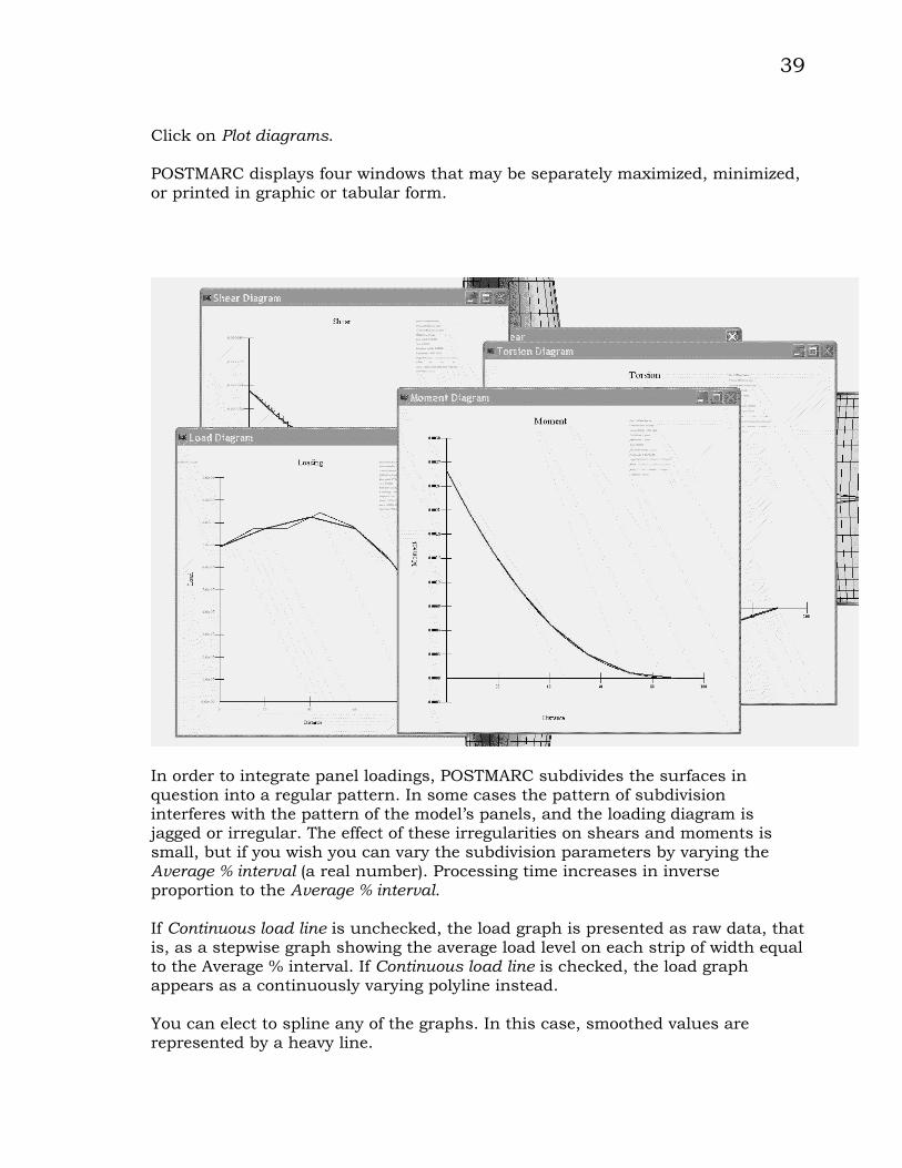
Click on Plot diagrams.

POSTMARC displays four windows that may be separately maximized, minimized,or printed in graphic or tabular form.

In order to integrate panel loadings, POSTMARC subdivides the surfaces inquestion into a regular pattern. In some cases the pattern of subdivisioninterferes with the pattern of the model’s panels, and the loading diagram isjagged or irregular. The effect of these irregularities on shears and moments issmall, but if you wish you can vary the subdivision parameters by varying theAverage % interval (a real number). Processing time increases in inverseproportion to the Average % interval.

If Continuous load line is unchecked, the load graph is presented as raw data, thatis, as a stepwise graph showing the average load level on each strip of width equalto the Average % interval. If Continuous load line is checked, the load graphappears as a continuously varying polyline instead.

You can elect to spline any of the graphs. In this case, smoothed values arerepresented by a heavy line.

40

To save all of the results at a specified interval in tabular form, enter an intervaland click on To File, every.

Stability derivatives and lift curve slope using CMARC

Stability and other derivatives are most easily obtained using DIGITAL WINDTUNNEL, but a simplified version of the procedure can also be run manually.

To obtain stability derivatives for aircraft, it is necessary first of all to run cases attwo angles of attack. For the sake of example longitudinal stability is used here,but the procedure for obtaining yaw and roll derivatives is analogous. (Note thatto obtain yaw derivatives you must model the complete airframe, settingRSYM=1.0 on the basic input page and IPATCOP=1 for all patches. Wakes mustbe explicitly defined for mirrored panels; CMARC has no facility for mirror-copyingwakes.)

A matrix of yaw and pitch cases can be run using CMARC's batch capability.

Since CMARC yields linear variations of moments with respect to angles of attack,it is not necessary to run more than two cases to obtain a result for any givenparameter; but additional cases at different angles may be run to average outslight variations or to observe the effect of different yaw angles on longitudinalstability or vice versa.

To obtain the lift curve slope, obtain CLs at two angles of attack, preferably onedegree apart.

The procedure for obtaining longitudinal stability derivatives is similar. Note thevalue of C_m for two different angles of attack. The difference between the twocoefficients, divided by the difference in angles of attack, is the stability derivativefor a CG position represented by the coordinates of the Moments relative to point.

To obtain yawing stability derivatives or rolling moments as a function of yaw, usea similar procedure with the values of C_n or C_l. Note that coefficients arereported with respect to both wind and body axes. Normally, the values withrespect to wind axes should be used.

Maximum roll rate may be obtained with a fully defined bilaterally symmetricalmodel by setting the maximum deflection into the ailerons. Run two analyses, onewith zero roll rate and one with, say, 100 deg/sec roll rate. The rolling momentcoefficient diminishes as the roll rate increases, and the point at which the rollingmoment is zero is the maximum roll rate.

41

Note that the roll rate is really a helix angle. If the roll rate is entered as its realvalue, eg 100 deg/sec, then the speed (VINF) must have its real value as well. IfVINF is 1.0, then the roll rate must be divided by the speed to obtain aproportionally correct value.

An empirical correction (found in Hoerner, Fluid Dynamic Lift, and appliedautomatically by DWT) must be applied to convert the roll rate obtained into arealistic one. Rates obtained from POSTMARC are useful for comparing variousconfigurations, but not for predicting actual roll rates.

Neutral point

To obtain the longitudinal static neutral point, use two cases with angles of attackdiffering by one degree. For each case, note C_m, then move the X coordinate ofthe moment reference point an appropriate distance aft and note C_m again. Bysubtracting the corresponding values and dividing by the distance betweenstations, obtain the slope of C_m with respect to alpha for two moment referencepoints. For longitudinally stable configurations, the more aft location of themoment reference point will correspond to the lesser of the two slopes.

Next, convert the slopes to angles by taking their arctangents.

Finally, obtain the neutral point by extrapolating from the angles to the station atwhich the angle would be zero. This may be done using interpolation utility (in theMisc menu) in LOFTSMAN.

Elevator angle to trim

A similar procedure may be used to determine elevator angle to trim at a givenangle of attack and CG location. Use the CG location as the moment referencepoint and run analyses at two values of elevator tilt, preferably bracketing theexpected one.

Stability analysis with DWT

All procedures related to static stability, trim, neutral point and roll rate areperformed automatically, and with greater refinement, by DIGITAL WINDTUNNEL, AeroLogic's Windows executive for CMARC. DWT also predicts dynamicstability rates and convergence/divergence.

42

Inertial calculation

For calculation of dynamic stability with DIGITAL WIND TUNNEL, it is necessaryto provide moments of inertia for the complete model. POSTMARC incorporates aprocedure for doing this.

Select

Calculations > Inertial properties

A form for estimating inertial properties appears.

POSTMARC recognizes two categories of items contributing to moments of inertia:first, discrete, concentrated masses, and second, the surface of the model.

Inertia of discrete components

At the top of the Calculate Inertial Properties form is a box containing a scrollingmaster list of items contributing to the mass of the model. To add items to the list,enter their names, masses, and the coordinates of their centroids in the areacaptioned Item Inertial Properties. When you have defined an item, click on Additem to list. You can save the list at any time by clicking on Write File, and you canimport an existing list with Read File. You can also delete individual items or allitems in the list.

To compute the inertial properties of items on the list, you must provide amoment reference point. This point normally corresponds to a design CG location,and its coordinates are usually stored in the CMARC input file as RMPX, RMPY,and RMPZ. To retrieve these values from the current CMARC input file, click onLoad .in. If the name of the appropriate input file is different from that of thecurrent file, you must type it in the adjacent box before pressing Load .in.

The area captioned Calculated Properties delivers the aggregated mass, moment ofinertia, and center of gravity of all components in the master list. Note that if themaster list is fairly complete, it serves as a weight and CG buildup for thecomplete aircraft or vessel.

Note also that POSTMARC slightly underestimates total moments of inertia,because it does not take into account the rotational moments of inertia ofindividual components about their own centroids. For example, POSTMARCwould find zero moments of inertia for an engine whose mass centroid coincides

43

with the moment reference point, but the engine would, in fact, contribute somedamping to pitch, yaw and roll rates. If you wish to take these moments intoaccount, you can enter moments manually in the Item Inertial Properties area.

Inertia of the model surface

The model surface is addressed in the area captioned Patch Inertial Properties. Theapproximate moment of inertia of the highlighted patches is obtained by enteringan average value for the mass per unit of area of the surface and clicking onCalculate Inertial Properties. For example, the mass of .032 aluminum sheet isabout .00323 pounds per square inch. By default, all surface patches areincluded; but you can obtain moments of inertia for portions of the surface byselecting or deselecting patches in the list box.

To add all or part of the surface to the master input list, provide a name and aWeight/Area ratio for it and click on Add Item to List. Be sure that theWeight/Area ratio is in units consistent with those used to define the model.

45

9. Output options

Hard copy

To obtain printed copies of screen displays, select File > Print. Use File > Print setupto gain access to the standard Windows printer setup forms.

POSTMARC will not print wakes that are being continuously generated by thewake animation routine.

Saving to the clipboard

Screen images can also be saved in the Windows Clipboard. Hit <Alt-PrtSc>.The current screen (including the toolbar) will be moved to the Clipboard.

POV-Ray

POV-Ray is short for Persistence of Vision Raytracer, a tool for producing high-quality computer graphics. POV-Ray is copyrighted freeware and can bedownloaded from the World Wide Web at www.povray.org. Examples of POV-Rayrendered models can also be seen on the AeroLogic web page atwww.aerologic.com.

To make a POV-Ray file of the current view, select

File > Export > POV-Ray

to create and name a file.

POSTMARC writes out every panel on a patch by patch basis. Each four-sidedpanel in the POSTMARC input model is broken into two triangles to conform tothe "mesh of triangles" format of POV-Ray. POSTMARC assigns a different textureor color for each patch. The camera direction (or view position) is stored in thePOV-Ray file. The POV-Ray deck can be manually edited in order to modify

46

textures and/or colors for each patch. Items such as landing gear, propellers, etc.can be added in order to make photorealistic pictures.

In general, what is saved in POV-Ray format is what you see on the screen inPOSTMARC. If only half a model is displayed, only that half of the model will besaved.

VRML

VRML is an acronym for Virtual Reality Modeling Language. VRML allows you todescribe 3D objects and combine them into scenes and "worlds." You can useVRML to create interactive simulations that incorporate animation, motionphysics, and real-time multi-user participation.

To save a wireframe geometry, select

File > Export > VRML

POSTMARC will prompt you for a name and create a VRML file. As with POV-Rayfiles, only the portions of the model actually displayed on the screen will be saved.The default file extension is .WRL (for "world").

Models can also be saved as colored surfaces representing any of the contourablevariables computed by CMARC or POSTMARC. Select

Display > Contour solid (VRML)

Evaluation copies of a VRML viewer, CosmoPlayer, can be downloaded from theweb site at www.vrml.sgi.com. Examples of POSTMARC-generated VRML outputcan be seen on the AeroLogic web page at www.aerologic.com.

DXF

DXF is a graphics data storage format originated by the creators of AutoCAD andnow supported by most CAD systems. POSTMARC will save the current model (asdisplayed on the screen) in DXF "mesh" format, which allows most CAD programsto perform hidden line removal and rendering.

Select

File > Export > DXF

47

The output file has a .DXF extension. As with other geometry-filing formats, onlythe portion of the model displayed on the screen will be saved.

11/6/2013

pm doc

Documents