plumes and thermalscushman/books/efm/chap10.pdf164 chapter10. plumes figure 10.1: a hydrothermal...
TRANSCRIPT
Chapter 10
Plumes and Thermals
SUMMARY: This chapter describes several distinct structures that fluids developin reaction to localized inputs of buoyancy. A punctual and sustained source ofbuoyancy usually creates a continuous rise of lighter fluid through the ambientdenser fluid, with mixing occurring along the way. Such structure is called a plume.Should the process be intermittent, the rising buoyant fluid parcels are called ther-
mals. Buoyant jets are plumes with the added propulsion of momentum, and buoy-
ant puffs are fluid parcels that rise under the combined action of buoyancy andmomentum.
10.1 Plumes
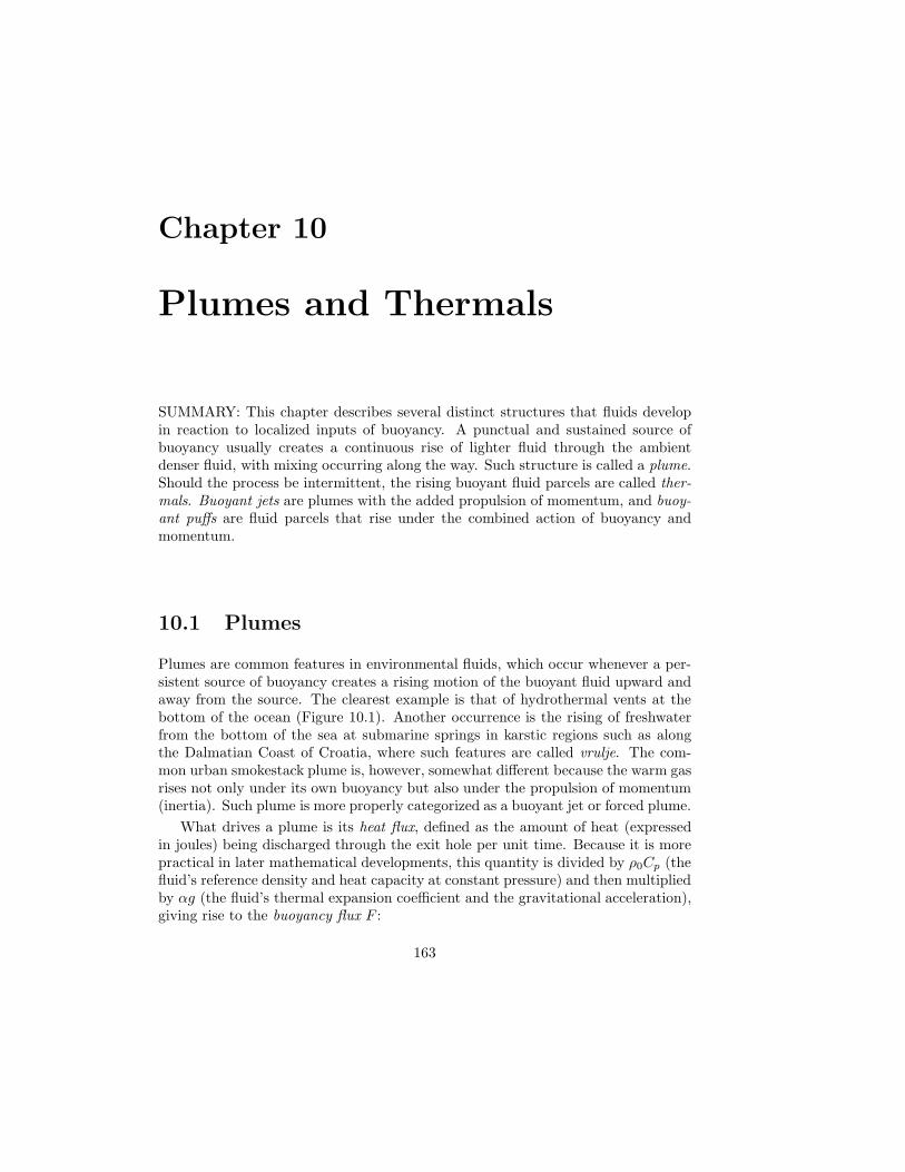
Plumes are common features in environmental fluids, which occur whenever a per-sistent source of buoyancy creates a rising motion of the buoyant fluid upward andaway from the source. The clearest example is that of hydrothermal vents at thebottom of the ocean (Figure 10.1). Another occurrence is the rising of freshwaterfrom the bottom of the sea at submarine springs in karstic regions such as alongthe Dalmatian Coast of Croatia, where such features are called vrulje. The com-mon urban smokestack plume is, however, somewhat different because the warm gasrises not only under its own buoyancy but also under the propulsion of momentum(inertia). Such plume is more properly categorized as a buoyant jet or forced plume.
What drives a plume is its heat flux, defined as the amount of heat (expressedin joules) being discharged through the exit hole per unit time. Because it is morepractical in later mathematical developments, this quantity is divided by ρ0Cp (thefluid’s reference density and heat capacity at constant pressure) and then multipliedby αg (the fluid’s thermal expansion coefficient and the gravitational acceleration),giving rise to the buoyancy flux F :
163

164 CHAPTER 10. PLUMES
Figure 10.1: A hydrothermal vent at the bottom of the Pacific Ocean, discharginghot water (up to 400◦C) and forming a vertical plume. The dark color, giving rise tothe nickname black smoker, is due the presence of sulfides in the water. [Photographtaken by Dudley Foster, courtesy of the Woods Hole Oceanographic Institution]
F =αg
ρ0Cp
heat
time. (10.1)
Note that because heat per time is expressed in J/s, the buoyancy flux is measuredin units of m4/s3.
Let us consider a three-dimensional radially symmetric plume progressing verti-cally from the bottom through a homogeneous and resting fluid, as shown in Figure10.2. If we denote by T0 the temperature of the ambient fluid, then the tempera-ture inside the plume has the value T0 + T ′, in which T ′ denotes the temperatureanomaly (positive in a rising plume, negative in a sinking plume). To this temper-ature anomaly corresponds a density anomaly ρ′ = −αρ0T
′. From the latter, it isconvenient to define the local buoyancy, or reduced gravity, g′ as:
g′ = − gρ′
ρ0= + αgT ′. (10.2)
Naturally, because of the heterogeneous structure of the plume, with entrainmentand dilution taking place along its sides, the buoyancy g′ and vertical velocity wwithin the plume depend on both distance z above the source and radial distance rfrom the centerline. Like for turbulent jets (previous chapter), observations revealthat the Gaussian profile (bell curve) provides a realistic description of the statisticalaverages of g′ and w over the turbulent fluctuations. Before using such expressions,however, we shall initially limit ourselves to considering only cross-plume averagesw and g′, each a function of z, the height within the plume.
The buoyancy flux F can be expressed as the integral across the section of theplume of the product of the vertical velocity w with the buoyancy g′. In terms of
10.1. PLUMES 165
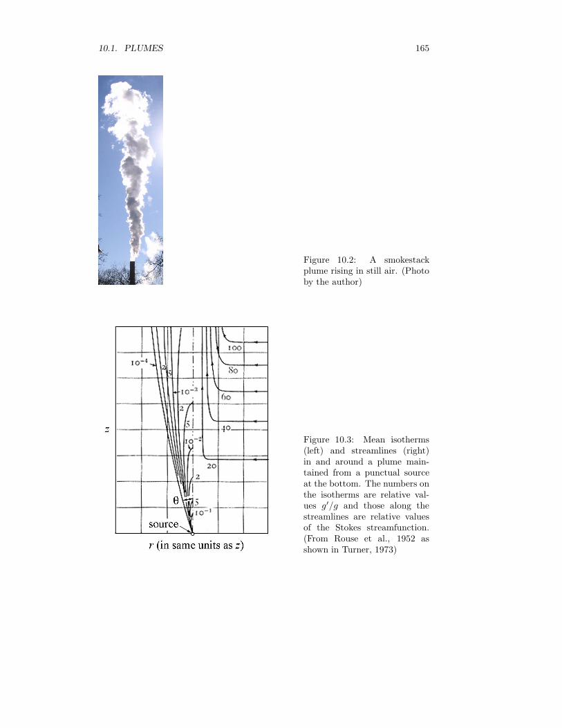
Figure 10.2: A smokestackplume rising in still air. (Photoby the author)
Figure 10.3: Mean isotherms(left) and streamlines (right)in and around a plume main-tained from a punctual sourceat the bottom. The numbers onthe isotherms are relative val-ues g′/g and those along thestreamlines are relative valuesof the Stokes streamfunction.(From Rouse et al., 1952 asshown in Turner, 1973)

166 CHAPTER 10. PLUMES
the mean values across the plume, a reasonably good approximation is
F = πR2 wg′ = πR2 αgT ′w, (10.3)
where R(z) is the radius of the plume at level z.As the plume rises, it entrains ambient fluid, but this does not change the heat
flux carried by the plume since that ambient fluid carries no heat anomaly. Thus,by virtue of conservation of heat, the buoyancy flux remains unchanged with heightand is the same at level z as it was at the start of the plume. In other words, thequantity F is constant. It is what drives the plume, like momentum drives a jet.
Figure 10.4: A thin slide ofthe plume on which to performmass and momentum budgets.
Perfoming a mass conservation budget over a thin slice of the plume extendingfrom level z to level z + dz (Figure 10.4), we can write:
Mass exiting from the top = Mass entering through the bottom
+ Mass entrained through the side.
[πR2 ρ0w]z+dz = [πR2 ρ0w]z + 2πRdz ρ0u,
in which u is the lateral entrainment velocity and 2πRdz the lateral area of the slice(Figure 10.4). In differential form, this equation becomes
d
dz(R2w) = 2Ru. (10.4)
Likewise, the vertical momentum budget over the same slice requires
Momentum exiting from the top = Momentum entering through the bottom
+ Momentum entrained through the side
+ Upward buoyancy force.
There is no vertical momentum acquired by lateral entrainment since the ambientfluid is at rest. By virtue of Archimedes’ principle, the upward buoyancy force isequal to the weight of the displaced fluid (at density ρ0) minus the actual weight ofthe plume segment (at lower density ρ0 + ρ′), for a total of
10.1. PLUMES 167
Upward buoyancy force = πR2 ρ0 g dz − πR2 (ρ0 + ρ′) g dz
= −πR2 ρ′ g dz
= +πR2 ρ0 g′ dz,
by virtue of (10.2). Thus, the vertical momentum budget takes the form:
[πR2 ρ0w2]z+dz = [πR2 ρ0w
2]z + πR2 ρ0g′ dz,
or, in differential form,
d
dz(R2 w2) = R2 g′. (10.5)
Let us stop for a moment and take stock of the equations we have. There arethree equations: (10.3) from the heat budget, (10.4) from the mass budget, and(10.5) from the momentum budget. And, there are four unknowns: the radius R,the average velocity w, the entrainment velocity u, and the averaged buoyancy g′,each a function of the elevation z. There is thus one more unknown than availableequations. To close the problem without solving for the details of the turbulentflow, we state in analogy with the turbulent jet, that the entrainment velocity isproportional to the shear flow induced by the plume. In other words, we assumeproportionality between u and w:
u = a w, (10.6)
with constant dimensionless coefficient a.The solution of the problem ought to be expressed solely in terms of the quan-
tities F (in m4/s3) and z (in m), because those are the only dimensional variablesentering the equations. Thus, dimensional considerations lead us to anticipate theform of the solution:
R = tan θ z
w = bF 1/3
z1/3
g′ = cF 2/3
z5/3,
where θ is the angle of the cone made by the plume (Figure 10.3). Observations(Turner, 1973) indicate that this angle is about 8.9◦, for which tan θ = 0.157.
Substitution in the equations at our disposal yields:
Eq. (10.3) −→ πbc tan θ = 1
Eq. (10.4) −→5
3tan θ = 2a
Eq. (10.5) −→4
3b2 = c.

168 CHAPTER 10. PLUMES
The values of the dimensionless coefficients are found to be
a =5
6tan θ = 0.1305
b =
(
3
4π tan2 θ
)1/3
= 2.14
c =
(
4
3π2 tan4 θ
)1/3
= 6.08
and the assembled solution is
R = 0.157 z (10.7)
w = 2.14F 1/3
z1/3(10.8)
u = 0.130 w = 0.279F 1/3
z1/3(10.9)
g′ = 6.08F 2/3
z5/3. (10.10)
Let us now pass from w and g′ averaged across the plume to functions w and g′
with Gaussian profile across the plume. For this, we write:
w = wmax(z) exp
(
−r2
2σ2
)
(10.11)
g′ = g′max(z) exp
(
−r2
2σ2
)
, (10.12)
with the standard deviation σ(z) being such that 2σ(z) represents the radius R(z)of the plume at height z. (See theory for the turbulent jet in the previous chapter.)Thus, σ = R/2. The peak values along the plume’s centerline can then be relatedto their respective averages by
w =1
πR2
∫
∞
0
w 2πrdr (10.13)
g′ =1
πR2
∫
∞
0
g′ 2πrdr, (10.14)
and we obtain:
w = 4.27F 1/3
z1/3exp
(
−81.6r2
z2
)
(10.15)
g′ = 12.2F 2/3
z5/3exp
(
−81.6r2
z2
)
. (10.16)
10.2. PLUMES IN STRATIFICATION 169
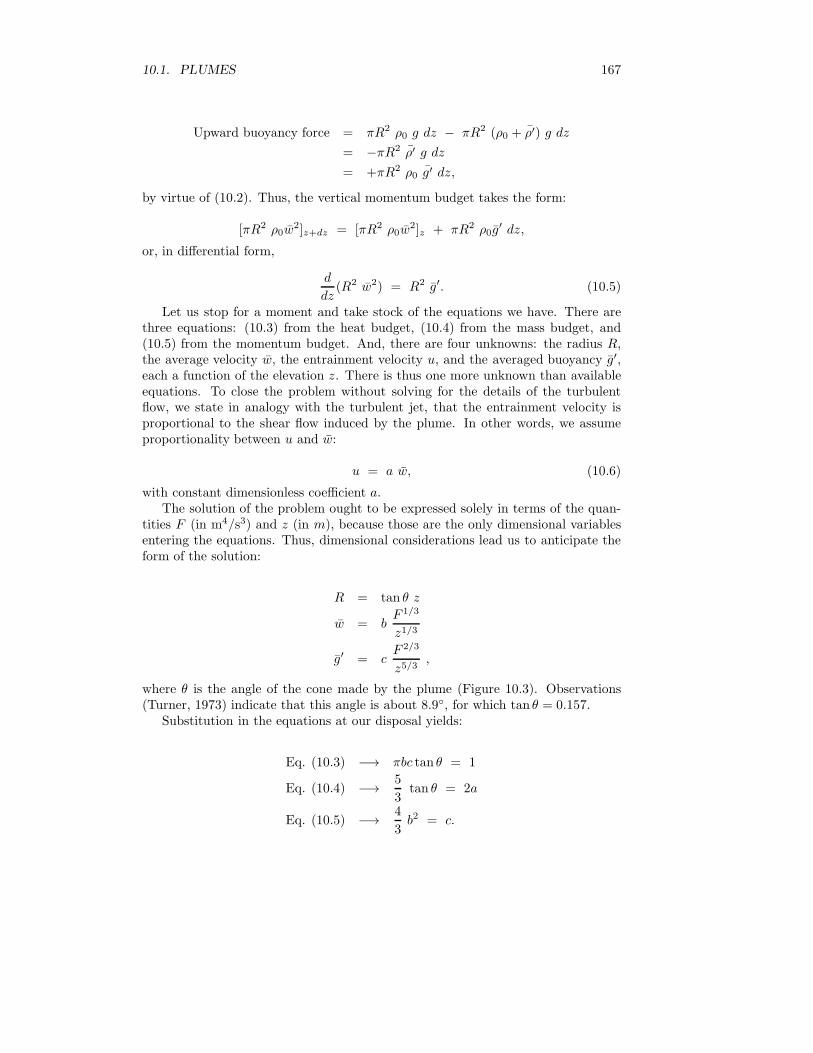
Figure 10.5: A plume rising in an early morning when the lower atmosphere isstratified. A clue of this stratification is the thin horizontal band of cloud on theleft of the plume (marked in picture). Note the inertial overshoot of the plumecloud before settling at the level of neutral buoyancy. [Photograph by the author]
Laboratory experiments (Turner, 1973), indicate that the following adjustedexpressions
w = 4.7F 1/3
z1/3exp
(
−96r2
z2
)
(10.17)
g′ = 11F 2/3
z5/3exp
(
−71r2
z2
)
(10.18)
better match the observations. Note that with these last expressions, the width ofthe velocity profile is slightly narrower than that of the buoyancy.
10.2 Plumes in a Stratified Environment
When a plume rises (or sinks) in a stratified environment, it encounters a tempera-ture becoming closer to its own and progressively loses buoyancy. At some level, itwill have lost all buoyancy and will begin to spread horizontally. Such is the caseof a smokestack plume in a calm (no wind) and stratified atmosphere typical ofthe early morning (Figure 10.5). The obvious question to ask is how high does theplume reach?
The stratified ambient fluid is characterized by its stratification frequency Ndefined from
N2 = αgdT
dz(10.19)

170 CHAPTER 10. PLUMES
where T (z) is the temperature profile of the ambient fluid.To describe a plume in this type of environment, the same quantities are needed
as before, namely the plume’s radius R, averaged vertical velocity w, and averagedbuoyancy g′, each function of the elevation z. The difference with the previoussection is that now the buoyancy flux F , defined in (10.3), is no longer a constantalong the axis of the plume. Three equations are at our disposal: The mass budget
d
dz(wR2) = 2uR = 2awR, (10.20)
the momentum budget
d
dz(w2R2) = g′ R2, (10.21)
which remain unchanged, and the heat budget, which is
d
dz(wTplume πR2) = uT (z) 2πR. (10.22)
Using the buoyancy locally experienced by the plume, g′ = αg[Tplume − T (z)], thelast equation can be recast as
d
dz(g′wR2) +
d
dz[αgT (z) wR2] = 2uR αgT (z).
With Equation (10.20) and definition αg dT (z)/dz = N2, it can be reduced to
d
dz(g′wR2) = −N2 w R2. (10.23)
The solution to this set of equations does not exhibit similarity, but the equationscan easily be integrated numerically. Starting with initial conditions (at level z = 0)such that the momentum and volumetric flow are nil but buoyancy flux finite, onefinds the results shown in Figure 10.6. On that figure, the variables are madedimensionless by scaling as follows: z and R by (F/N3)1/4, w by (F/N)1/4, and g′
by (F/N5)1/4, where F is the starting buoyancy flux (at z = 0). The entrainmentparameter a was taken as 0.125. (For a similar numerical integration, see Morton,Taylor and Turner, 1956).
We note on Figure 10.6 that the buoyancy crosses zero at z = 2.98(F/N3)1/4,but the residual vertical velocity at that level makes the plume overshoot, up toz = 3.92 (F/N3)1/4, by which level the vertical velocity vanishes and the radiusbecomes infinite.
Laboratory experiments and field observations confirm and tweak this theoreti-cal prediction (Figure 10.7). Briggs (1969) gives
zmax = 5.0
(
F
πN3
)1/4
= 3.76
(
F
N3
)1/4
. (10.24)

10.3. THERMALS 171
Figure 10.6: Numerical inte-gration of Equations (10.20),(10.21) and (10.23), with a =0.125, tracing the vertical struc-ture of a buoyant plume asit rises in a stratified environ-ment. The buoyancy crosseszero at z = 2.98, above whichthe plume becomes negativelybuoyant. The vertical veloc-ity vanishes at z = 3.92 andthe radius becomes infinite. Seetext for details of the non-dimensionalization employed inmaking the graph.
10.3 Thermals
A thermal is a finite parcel of fluid consisting of the same fluid as its surroundingsbut at a different temperature. Because of its buoyancy, a cold thermal sinks (neg-ative buoyancy), while a warm thermal rises (positive buoyancy). The name wasgiven by glider pilots to what they perceived as regions of warm air rising above aheated ground in which they could soar. Convection in the atmosphere does indeedproceed by means of rising thermals (Priestley, 1959). The situation, however, canbe quite chaotic, with a collection of thermals rising here and there at various times,some of them smaller and slower, and others larger and faster. Here, for the sakeof understanding the basic mechanism, we shall be concerned with a single thermalimmersed in an infinite homogeneous fluid at rest.
Experiments have been conducted in the laboratory (Figure 10.8), and it hasbeen found that all thermals roughly behave in similar ways: as they rise (or sink),they entrain surrounding fluid and become more dilute, thereby slowing down intheir ascent (or descent). The actual shape of a thermal, however, can vary consid-erably from one set of observations to another. Here, basic dynamics supplementedby a few dimensionless numbers gleaned from experiments will be used to establisha simple theory for the prediction of a thermal’s behavior over time.
The key property of a thermal is its total buoyancy, defined as
B = αgT ′V = g′V (10.25)
in which V is the volume of the thermal, T ′ its temperature anomaly, and g′ = αgT ′
the reduced gravity it experiences. This total buoyancy is a conserved quantity asthe thermal rises (or sinks) because, while it entrains surrounding fluid, its tem-perature anomaly decreases by dilution in proportion to its volume increase, thuskeeping the product T ′V constant during the thermal’s life.

172 CHAPTER 10. PLUMES
Figure 10.7: Measurements ofplume rise in calm stratifiedsurroundings, revealing that theultimate height reached by aplume follows Equation (10.24).(Adapted from Briggs, 1969)
The volume of a thermal can be expressed as
V = mR3, (10.26)
where R is the radius of the thermal seen from above, and m is a coefficient lessthat 4π/3 = 4.2 (value for a spherical volume) because a thermal has a slightlyflattened shape. The value ofm is notoriously difficult to measure, and some indirectmeasurement is in order, as we shall see later.
Mass conservation over time can be expressed as
dV
dt= Au,
in which A is the enclosing surface area of the thermal and u the average entrainmentvelocity across that surface (Figure 10.9). Taking the area A as proportional to R2,the square of the thermal’s radius, and the entrainment velocity u as proportionalto the thermal’s vertical velocity w, we can express the preceding equation as
dV
dt= aR2w, (10.27)
in which the coefficient a ought to be a dimensionless constant, to be determinedfrom experiments or observations. Using (10.26), this equation can be reduced to:
dR
dt=
a
3mw. (10.28)
The momentum budget over time takes the form
d
dt
(
3
2ρthermalV w
)
= Upward buoyancy force − Downward weight

10.3. THERMALS 173
Figure 10.8: Descending thermals in a laboratory experiment. These thermals inwater are made visible by barium sulfate. The stem left behind by each thermal isdue to the manner a spherical cap was rotated to provoke the release. The secondthermal (bottom row) has a larger negative buoyancy than the first (top row). [FromScorer, 1997]
= ρambient V g − ρthermal V g
= ρthermal αT′ V g
= ρthermal g′V,
in which the factor 3/2 on the left is due to the added-mass effect. Physically, thethermal is subject to its own acceleration (time derivative of one time ρthermalV w),but its changing pace also causes acceleration of the surrounding fluid diverted byits passage, effectively accelerating 50% more fluid mass, hence the factor 3/2 = 1.5.Division by ρthermal, which at all times remains close to the reference density of thefluid, yields
d
dt(V w) =
2
3g′V. (10.29)
Elimination of the product g′V by virtue of Equation (10.25) indicates that theright-hand side of the preceding equation is a constant, leading to an immediateintegration:
V w =2
3B t, (10.30)
for which t = 0 marks the time when the thermal had zero momentum. Next,
174 CHAPTER 10. PLUMES
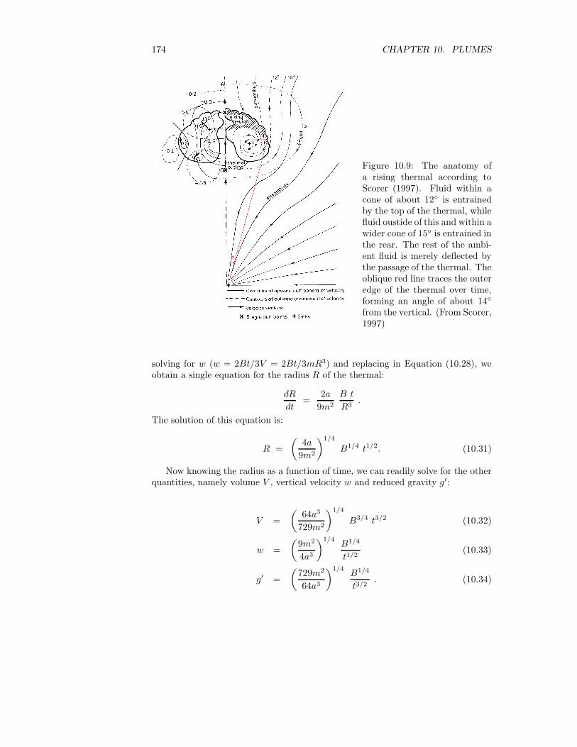
Figure 10.9: The anatomy ofa rising thermal according toScorer (1997). Fluid within acone of about 12◦ is entrainedby the top of the thermal, whilefluid oustide of this and within awider cone of 15◦ is entrained inthe rear. The rest of the ambi-ent fluid is merely deflected bythe passage of the thermal. Theoblique red line traces the outeredge of the thermal over time,forming an angle of about 14◦
from the vertical. (From Scorer,1997)
solving for w (w = 2Bt/3V = 2Bt/3mR3) and replacing in Equation (10.28), weobtain a single equation for the radius R of the thermal:
dR
dt=
2a
9m2
B t
R3.
The solution of this equation is:
R =
(
4a
9m2
)1/4
B1/4 t1/2. (10.31)
Now knowing the radius as a function of time, we can readily solve for the otherquantities, namely volume V , vertical velocity w and reduced gravity g′:
V =
(
64a3
729m2
)1/4
B3/4 t3/2 (10.32)
w =
(
9m2
4a3
)1/4B1/4
t1/2(10.33)
g′ =
(
729m2
64a3
)1/4B1/4
t3/2. (10.34)

10.3. THERMALS 175
In these expressions, it is clear that the time origin actually refers to a virtual stagein which the thermal had zero volume, infinite velocity and infinite temperatureanomaly. Obviously, the actual life of the thermal started some finite time afterthis, with a finite volume, finite velocity and finite temperature anomaly.
Note that the complete solution depends on two dimensionless parameters, aand m. Since neither is easy to determine directly, it is wise to seek their valueindirectly by matching thermal’s properties that are more readily observed. Onesuch property is the manner in which the thermal’s radius grows with distance. Forthis, we integrate dz/dt = w to obtain the thermal’s elevation as a function of time.The result is:
z =
(
36m2
a3
)1/4
B1/4 t1/2. (10.35)
It appears that both elevation z and radius R grow at similar rates, yielding aconstant ratio:
R
z=
a
3m. (10.36)
Laboratory observations (Figure 10.9) reveal that this is indeed the case that ther-mals behave in a self-similar way, and that the ratio ofR to z is about tan 14◦ = 0.25.Thus,
R = 0.25 z, (10.37)
and a = 0.75m.
The other reliable observation is that the ratio z2/t (a time constant as predictedby the theory) varies from experiment to experiment in proportion to
√B (Figure
10.10). The theoretical coefficient of proportionality is√
36m2/a3, and experiments
give it a value of 5.80. Solving a = 0.75m together with√
36m2/a3 = 5.80 yields:a = 1.90 and m = 2.54. From this follow all other coefficients:
R = 0.60 B1/4 t1/2 (10.38)
V = 0.55 B3/4 t3/2 (10.39)
w = 1.20B1/4
t1/2(10.40)
z = 2.41 B1/4 t1/2 (10.41)
g′ = 1.81B1/4
t3/2. (10.42)

176 CHAPTER 10. PLUMES
Figure 10.10: Plot of the quan-tity z2/t (a time constant dur-ing the life of thermal) versusthe square root of the thermal’sbuoyancy. Each numbered dotrefers to a different laboratoryexperiment, and the solid lineshows the best linear fit. (FromScorer, 1997)
10.4 Thermals in a Stratified Environment
When a thermal rises (or sinks) in a stratified environment, it progressively encoun-ters a temperature closer to its own and therefore loses its buoyancy. Ultimately, itwill reach a level of no buoyancy and begin to spread laterally (Figure 10.11). Withno thermal contrast left, the thermal loses its identity. What is this ultimate level isnot an obvious question. Indeed, it can be easily established that the thermal willnever reach the level of its initial temperature. The reason is its partial dilution byentrainment of surrounding fluid (which changes as the thermal crosses isotherms)and its consequent dilution.
A practical application of this situation is the dumping of waste in a stratifiedbody of water: The dumped waste sinks from the surface, gradually mixes withsurrounding water during its fall, and eventually settles down at some intermediatedepth. The determination of that depth is crucial in water quality studies andpermitting
The stratified environment is characterized by its stratification frequency Ndefined from
N2 = αgdT
dz, (10.43)

10.4. THERMALS IN STRATIFICATION 177
Figure 10.11: A laboratory experiment of a thermal sinking in a stratified envi-ronment. Note the ultimate arrest and spreading of the thermal once it loses itsbuoyancy. (From Scorer, 1997)
where T (z) is the temperature profile of the ambient fluid.
To track a thermal in this environment, the same quantities are needed as before,namely the thermal’s radius R, volume V = mR3, vertical position z, verticalvelocity w = dz/dt, reduced gravity g′, and total buoyancy B = g′V . The differencewith the previous section is that now the total buoyancy B is no longer a constantof the motion. Three equations are at our disposal: The mass budget
dV
dt= Au = aR2w, (10.44)
the momentum budget
d
dt(V w) =
2
3g′V, (10.45)
which remain unchanged, and the heat budget, which is
d
dt(V Tthermal) = AuT (z) = aR2wT (z). (10.46)
Using the reduced gravity locally experienced by the thermal, g′ = αg[Tthermal −T (z)], the last equation can be recast as
d
dt(V g′) +
d
dt[V αgT (z)] = aR2w αgT (z).
Using (10.44) and the fact that dT (z)/dt = (dT/dz) × (dz/dt) = w (dT/dz), itreduces to
d
dt(V g′) = −N2V w. (10.47)
Eliminating V from Equations (10.44), (10.45) and (10.47) by using V = mR3
yields a set of three equations for the three unknowns R, w and g′:
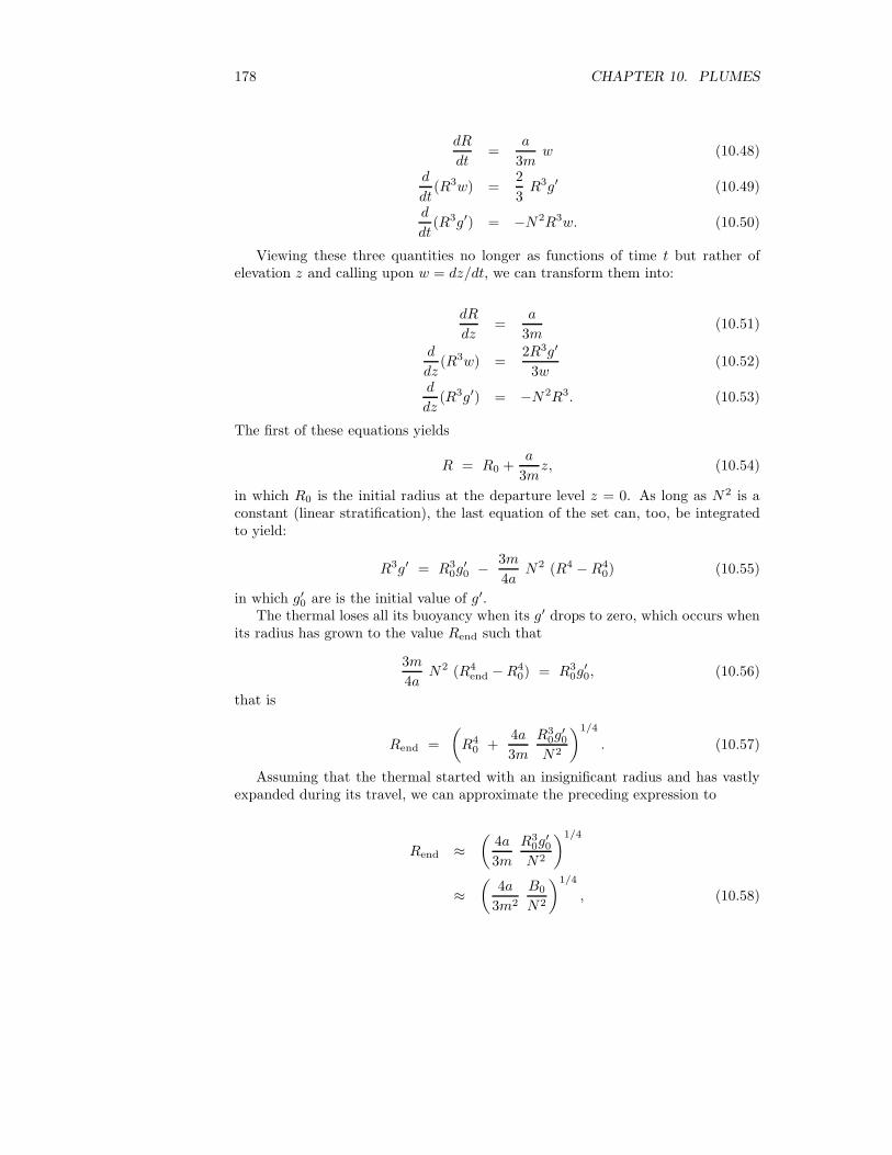
178 CHAPTER 10. PLUMES
dR
dt=
a
3mw (10.48)
d
dt(R3w) =
2
3R3g′ (10.49)
d
dt(R3g′) = −N2R3w. (10.50)
Viewing these three quantities no longer as functions of time t but rather ofelevation z and calling upon w = dz/dt, we can transform them into:
dR
dz=
a
3m(10.51)
d
dz(R3w) =
2R3g′
3w(10.52)
d
dz(R3g′) = −N2R3. (10.53)
The first of these equations yields
R = R0 +a
3mz, (10.54)
in which R0 is the initial radius at the departure level z = 0. As long as N2 is aconstant (linear stratification), the last equation of the set can, too, be integratedto yield:
R3g′ = R30g
′
0 −3m
4aN2 (R4 −R4
0) (10.55)
in which g′0 are is the initial value of g′.The thermal loses all its buoyancy when its g′ drops to zero, which occurs when
its radius has grown to the value Rend such that
3m
4aN2 (R4
end −R40) = R3
0g′
0, (10.56)
that is
Rend =
(
R40 +
4a
3m
R30g
′
0
N2
)1/4
. (10.57)
Assuming that the thermal started with an insignificant radius and has vastlyexpanded during its travel, we can approximate the preceding expression to
Rend ≈
(
4a
3m
R30g
′
0
N2
)1/4
≈
(
4a
3m2
B0
N2
)1/4
, (10.58)
10.5. PLUMES IN CROSS-FLOW 179
where B0 = V0g′
0 = mR30g
′
0 is the thermal’s initial buoyancy. Translating this radiusinto the corresponding elevation gives the terminal level where the thermal loses itsidentity:
zend =3m
a(Rend −R0) ≈
3m
aRend
≈
(
108m2
a3
)1/4 (
B0
N2
)1/4
. (10.59)
With the parameter values a = 1.90 and m = 2.54 determined at the end of theprevious section, we have
zend ≈ 3.17
(
B0
N2
)1/4
. (10.60)
Note that at the level where g′ = 0, the thermal has some residual vertical velocityand will overshoot slightly its level of neutral buoyancy. This explains the bulge onthe front side of the thermal seen in Figure 10.11.
10.5 Plumes in a Cross-Flow
The line thermal model.
Problems
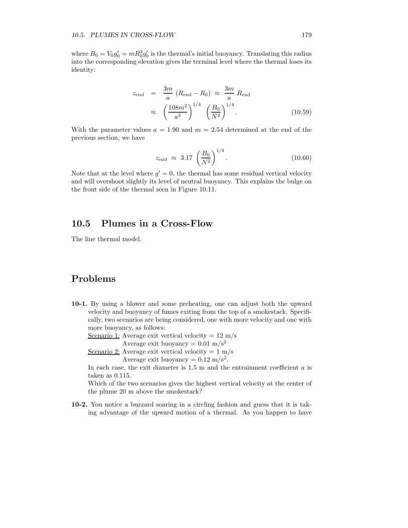
10-1. By using a blower and some preheating, one can adjust both the upwardvelocity and buoyancy of fumes exiting from the top of a smokestack. Specifi-cally, two scenarios are being considered, one with more velocity and one withmore buoyancy, as follows:Scenario 1: Average exit vertical velocity = 12 m/s
Average exit buoyancy = 0.01 m/s2
Scenario 2: Average exit vertical velocity = 1 m/sAverage exit buoyancy = 0.12 m/s2.
In each case, the exit diameter is 1.5 m and the entrainment coefficient a istaken as 0.115.Which of the two scenarios gives the highest vertical velocity at the center ofthe plume 20 m above the smokestack?
10-2. You notice a buzzard soaring in a circling fashion and guess that it is tak-ing advantage of the upward motion of a thermal. As you happen to have
180 CHAPTER 10. PLUMES
meteorological gear with you, including a radar profiler, you determine thatthe buzzard is flying at an altitude of 80 m and that the temperature at thecenter of the bird’s circle is 0.30◦C higher than outside the thermal, wherethe temperature is 25◦C.What is the radius of the thermal and its center vertical velocity? Also, howold is this thermal?
10-3.
10-4.
10-5. Show that, for a thermal rising in a homogeneous ambient fluid, w2 is equalto g′z/2. Does this relation have any particular significance?
10-6. Establish the form of the total energy of a thermal (kinetic plus potential) fora thermal rising in a uniform environment and determine its variation alongthe path of the thermal. Resolve any paradox.
10-7. It was mentioned at the end of the section on thermals in a stratified en-vironment that, once it reaches its level of neutral buoyancy, a thermal stillpossesses a residual vertical velocity. What is that velocity? And, at whatultimate level z does the vertical velocity finally vanish? Assume that theinitial radius of the thermal was negligible compared to its radius at the levelof neutral buoyancy.
10-8.
10-9.