plenoptic modeling: an image-based rendering system leonard mcmillan† and gary bishop †...
Post on 21-Dec-2015
216 views
TRANSCRIPT
Plenoptic Modeling:An Image-Based Rendering System
Leonard McMillan† and Gary Bishop †
Department of Computer Science
University of North Carolina at Chapel Hill
SIGGRAPH 95
Outline
Introduction The plenoptic function Previous work Plenoptic modeling
Plenoptic Sample Representation Acquiring Cylindrical Projections Determining Image Flow Fields Plenoptic Function Reconstruction
Results Conclusions
Introduction
In image-based systems the underlying data representation (i.e model) is composed of a set of photometric observations.
In computer graphics, the progression toward image-based rendering systems were texture mapping ,environment mapping ,and the images themselves constitute the significant aspects of the scene’s description.
Another reason for considering image-based rendering systems in computer graphics is that acquisition of realistic surface models is a difficult problem.
Introduction
One liability of image-based rendering systems is the lack of a consistent framework within which to judge the validity of the results. Fundamentally, this arises from the absence of a clear problem definition.
This paper presents a consistent framework for the evaluation of image-based rendering systems, and gives a concise problem definition.
We present an image-based rendering system based on sampling, reconstructing, and resampling the plenoptic function.
The plenoptic function
Adelson and Bergen [1] assigned the name plenoptic function to the pencil of rays visible from any point in space, at any time, and over any range of wavelengths.
The plenoptic function describes all of the radiant energy that can be perceived from the point of view of the observer rather than the point of view of the source.
They postulate “… all the basic visual measurements can be considered to characterize local change along one or two dimensions of a single function that describes the structure of the information in the light impinging on an observer.”

The plenoptic function
Imagine an idealized eye which we are free to place at any point in space(Vx, Vy, Vz).From there we can select any of the viewable rays by choosing an azimuth and elevation angle ( , ) as well as a band of wavelengths, , which we wish to consider.
FIGURE 1. The plenoptic function describes all of the image information visible from a particular viewing position.
θ φ

The plenoptic function
In the case of a dynamic scene, we can additionally choose the time, t, at which we wish to evaluate the function.
This results in the following form for the plenoptic function:
Given a set of discrete samples (complete or incomplete) from the plenoptic function, the goal of image-based rendering is to generate a continuous representation of that function.
Previous work
Movie-Maps Image Morphing View Interpolation Laveau and Faugeras Regan and Pose

Plenoptic modeling
We call our image-based rendering approach Plenoptic Modeling.
Like other image-based rendering systems, the scene description is given by a series of reference images.
These reference images are subsequently warped and combined to form representations of the scene from arbitrary viewpoints.
Plenoptic modeling
Our discussion of the plenoptic modeling image-based rendering system is broken down into four sections.
1. We discuss the representation of the plenoptic samples.
2. We discuss their acquisition.
3. Determinate image flow fields, if required.
4. We describe how to reconstruct the plenoptic function from these sample images.
Plenoptic Sample Representation
The most natural surface for projecting a complete plenoptic sample is a unit sphere centered about the viewing position.
One difficulty of spherical projections, however, is the lack of a representation that is suitable for storage on a computer.
This is particularly difficult if a uniform (i.e. equal area) discrete sampling is required.
Plenoptic Sample Representation
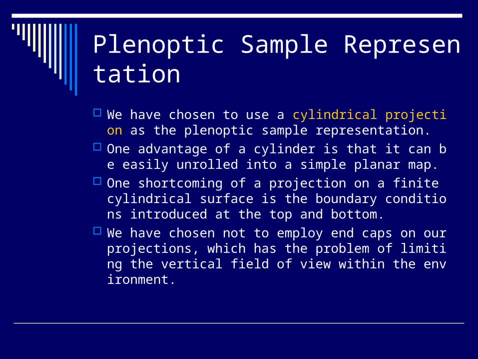
We have chosen to use a cylindrical projection as the plenoptic sample representation.
One advantage of a cylinder is that it can be easily unrolled into a simple planar map.
One shortcoming of a projection on a finite cylindrical surface is the boundary conditions introduced at the top and bottom.
We have chosen not to employ end caps on our projections, which has the problem of limiting the vertical field of view within the environment.

Acquiring Cylindrical Projections
A significant advantage of a cylindrical projection is the simplicity of acquisition.
The only acquisition equipment required is a video camera and a tripod capable of continuous panning.
Ideally, the camera’s panning motion would be around the exact optical center of the camera.
Acquiring Cylindrical Projections
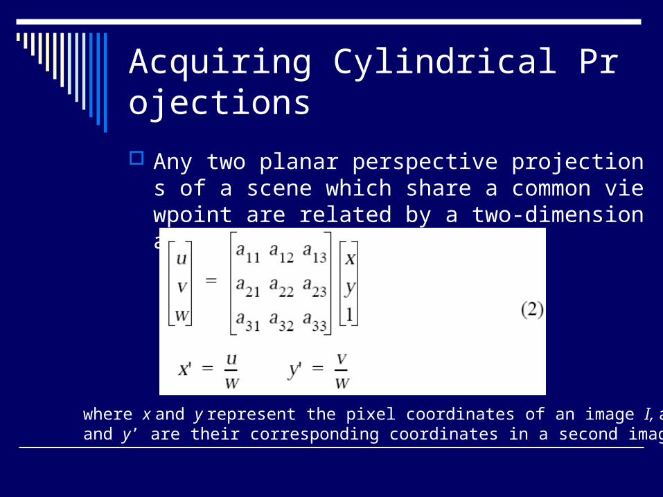
Any two planar perspective projections of a scene which share a common viewpoint are related by a two-dimensional homogenous transform:
where x and y represent the pixel coordinates of an image I, and x’and y’ are their corresponding coordinates in a second image I’.

Acquiring Cylindrical Projections
In order to reproject an individual image into a cylindrical projection, we must first determine a model for the camera’s projection or, equivalently, the appropriate homogenous transforms.
The most common technique [12] involves establishing four corresponding points across each image pair.
The resulting transforms provide a mapping of pixels from the planar projection of the first image to the planar projection of the second.
Acquiring Cylindrical Projections
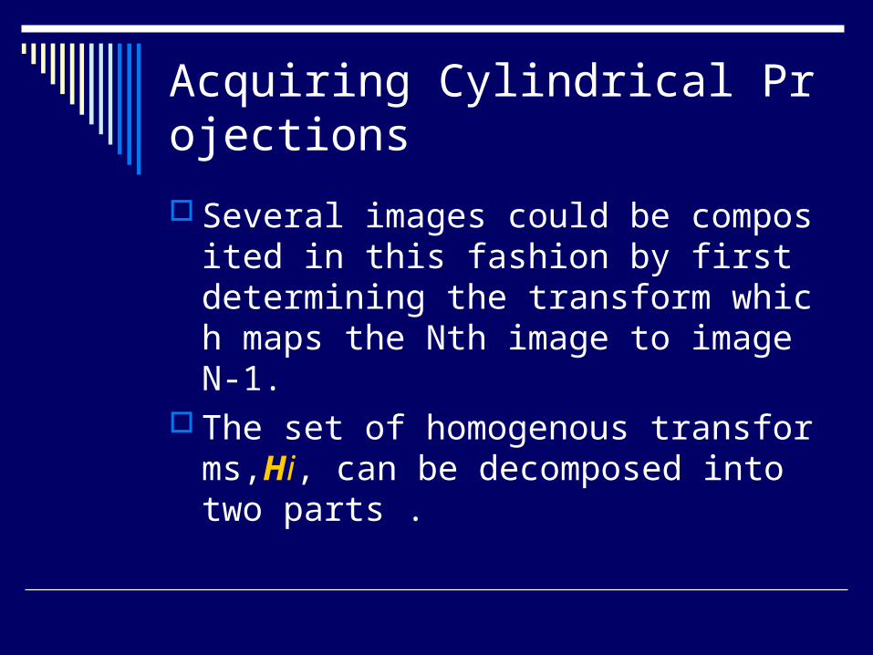
Several images could be composited in this fashion by first determining the transform which maps the Nth image to image N-1.
The set of homogenous transforms,Hi, can be decomposed into two parts .

Acquiring Cylindrical Projections
These two parts include an intrinsic transform, S, which is determined entirely by camera properties, and an extrinsic transform, Ri, which is determined by the rotation around the camera’s center of projection:

Acquiring Cylindrical Projections
The first step in our method determines estimates for the extrinsic panning angle between each image pair of the panning sequence.
This is accomplished by using a linear approximation to an infinitesimal rotation by the angle θ.
This linear approximation results from substituting 1 + O(θ2) for the cosine terms and θ+ O (θ3) for the sine terms of the rotation matrix.
Acquiring Cylindrical Projections
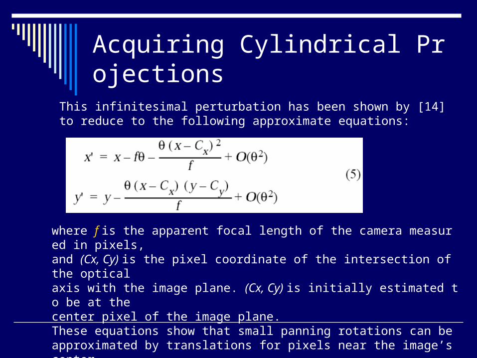
where f is the apparent focal length of the camera measured in pixels,and (Cx, Cy) is the pixel coordinate of the intersection of the opticalaxis with the image plane. (Cx, Cy) is initially estimated to be at thecenter pixel of the image plane.These equations show that small panning rotations can be approximated by translations for pixels near the image’s center.
This infinitesimal perturbation has been shown by [14] to reduce to the following approximate equations:

Acquiring Cylindrical Projections
The first stage of the cylindrical registration process attempts to register the image set by computing the optimal translation in x .
Once these translations, ti, are computed, Newton’s method is used to convert them to estimates of rotation angles and the focal length, using the following equation:
where N is the number of images comprising the sequence. This usually converges in as few as five iterations, depending on the o
riginal estimate for f.
Acquiring Cylindrical Projections
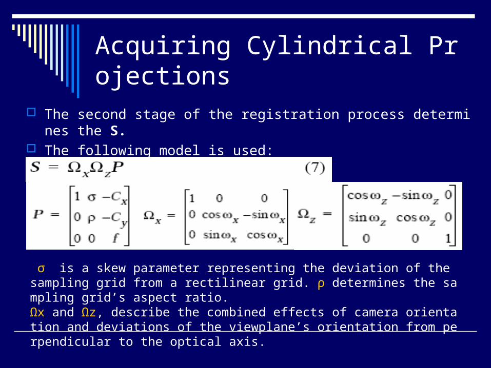
The second stage of the registration process determines the S. The following model is used:
σ is a skew parameter representing the deviation of the sampling grid from a rectilinear grid. ρ determines the sampling grid’s aspect ratio.Ωx and Ωz, describe the combined effects of camera orientation and deviations of the viewplane’s orientation from perpendicular to the optical axis.

Acquiring Cylindrical Projections
ωz term is indistinguishable from the camera’s roll angle and, thus, represents both the image sensor’s and the camera’s rotation. Likewise, ωx, is combined with an implicit parameter, φ, that represents the relative tilt of the camera’s optical axis out of the pan ning plane. If φ is zero, the images are all tangent to a cylinder and for a nonzero φ the projections are tangent to a cone.
This gives six unknown parameters, (Cx, Cy, σ, ρ, ωx, ωz), to be determined in the second stage of the registration process.

Acquiring Cylindrical Projections
The structural matrix, S, is determined by minimizing the following error function:
where Ii-1 and Ii represent the center third of the pixels from images i-1 and i respectively. Using Powell’s multivariable minimization method [23] with the following initial values for our six parameters,
the solution typically converges in about six iterations.

Acquiring Cylindrical Projections
The registration process results in a single camera model, S(Cx, Cy, σ, ρ, ωx, ωz, f ), and a set of the relative rotations, θi, between each of the sampled images. Using these parameters, we can compose mapping functions from any image in the sequence to any other image as follows:

Determining Image Flow Fields
Given two or more cylindrical projections from different positions within a static scene, we can determine the relative positions of centers-of-projection and establish geometric constraints across all potential reprojections.
These positions can only be computed to a scale factor.

Determining Image Flow Fields
To establish the relative relationships between any pair of cylindrical projections, the user specifies a set of corresponding points that are visible from both views.
These points can be treated as rays in space with the following form:
Ca =(Ax, Ay, Az) is the unknown position of the cylinder’s center of projection.
φa is the rotational offset which aligns the angu lar orientation of the cylinders to a common frame.
ka is a scale factor which determines the vertical field-of-view .
Cva is the scanline where the center of projection would project onto the scene
Determining Image Flow Fields
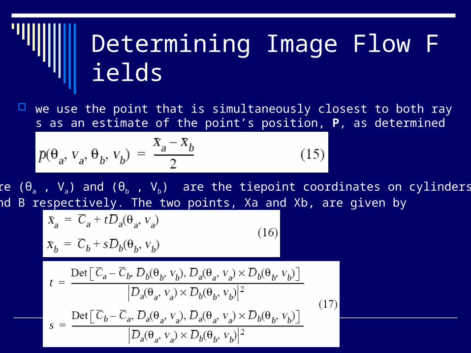
we use the point that is simultaneously closest to both rays as an estimate of the point’s position, P, as determined by the following derivation.
where (θa , Va) and (θb , Vb) are the tiepoint coordinates on cylindersA and B respectively. The two points, Xa and Xb, are given by

Determining Image Flow Fields
This allows us to pose the problem of finding a cylinder’s position as a minimization problem.
The position of the cylinders is determined by minimizing the distance between these skewed rays .
The use of a cylindrical projection introduces significant geometric constraints on where a point viewed in one projection might appear in a second.
We can capitalize on these restrictions when we wish to automatically identify corresponding points across cylinders.
Determining Image Flow Fields
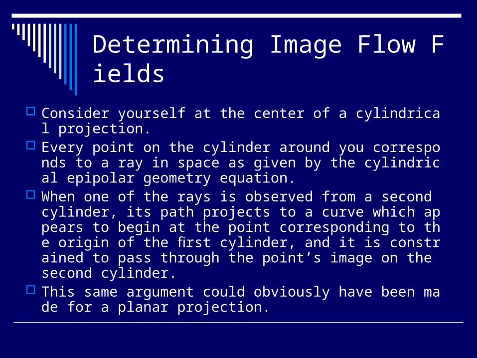
Consider yourself at the center of a cylindrical projection. Every point on the cylinder around you corresponds to a r
ay in space as given by the cylindrical epipolar geometry equation.
When one of the rays is observed from a second cylinder, its path projects to a curve which appears to begin at the point corresponding to the origin of the first cylinder, and it is constrained to pass through the point’s image on the second cylinder.
This same argument could obviously have been made for a planar projection.

Determining Image Flow Fields
The paths of these curves are uniquely determined sinusoids.
This cylindrical epipolar geometry is established by the following equation.

Plenoptic Function Reconstruction
FIGURE 2. Diagram showing the transfer of the knowndisparity values between cylinders A and B to a new viewing position V.
Plenoptic Function Reconstruction
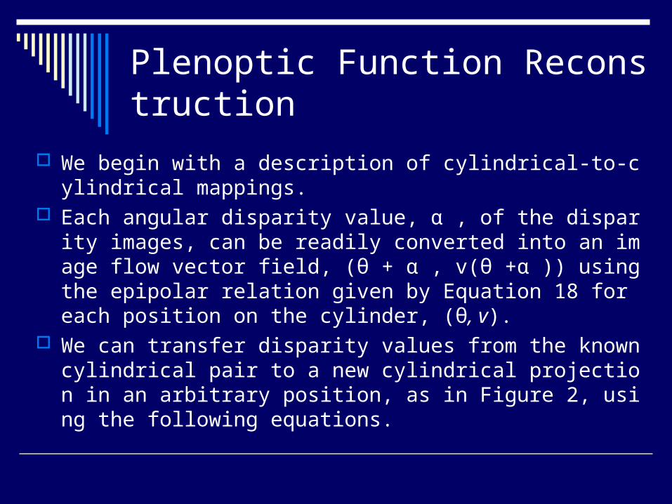
We begin with a description of cylindrical-to-cylindrical mappings.
Each angular disparity value, α , of the disparity images, can be readily converted into an image flow vector field, (θ + α , v(θ +α )) using the epipolar relation given by Equation 18 for each position on the cylinder, (θ, v).
We can transfer disparity values from the known cylindrical pair to a new cylindrical projection in an arbitrary position, as in Figure 2, using the following equations.
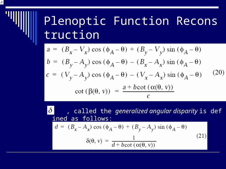
Plenoptic Function Reconstruction
, called the generalized angular disparity is defined as follows:
Plenoptic Function Reconstruction
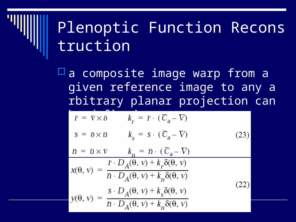
a composite image warp from a given reference image to any arbitrary planar projection can be defined as
Plenoptic Function Reconstruction
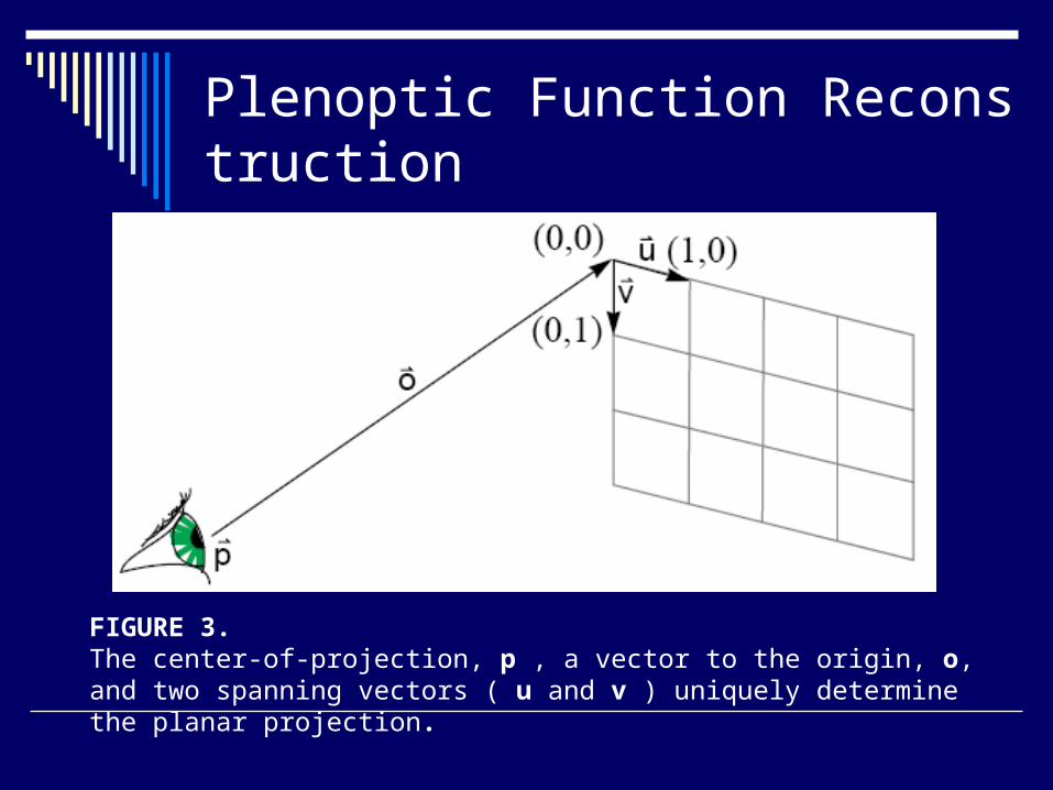
FIGURE 3. The center-of-projection, p , a vector to the origin, o, and two spanning vectors ( u and v ) uniquely determine the planar projection.

Plenoptic Function Reconstruction
Potentially, both the cylinder transfer and image warping approaches are many-to-one mappings.
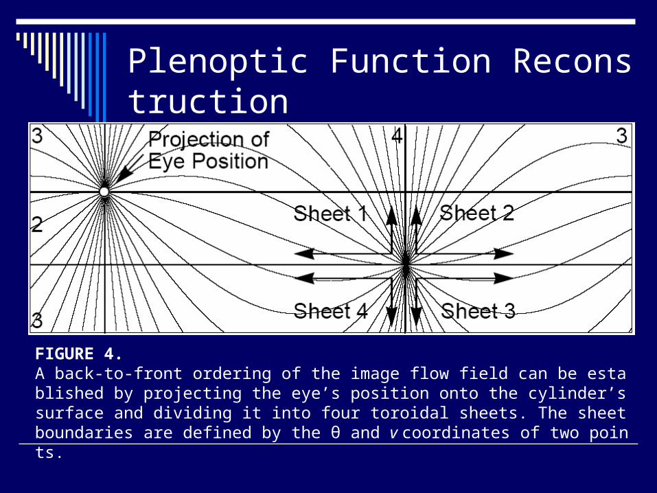
For this reason we must consider visibility. The following simple algorithm can be used to determine an enumeration of the cylindrical mesh which guarantees a proper back-to-front ordering.
We project the desired viewing position onto the reference cylinder being warped and partition the cylinder into four toroidal sheets.
Plenoptic Function Reconstruction
FIGURE 4. A back-to-front ordering of the image flow field can be established by projecting the eye’s position onto the cylinder’s surface and dividing it into four toroidal sheets. The sheet boundaries are defined by the θ and v coordinates of two points.

Results
We collected a series of images using a video camcorder on a leveled tripod in the front yard of one of the author’s home.
The autofocus and autoiris features of the camera were disabled, in order to maintain a constant focal length during the collection process.
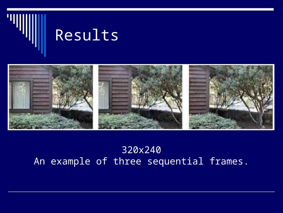
Results
320x240An example of three sequential frames.
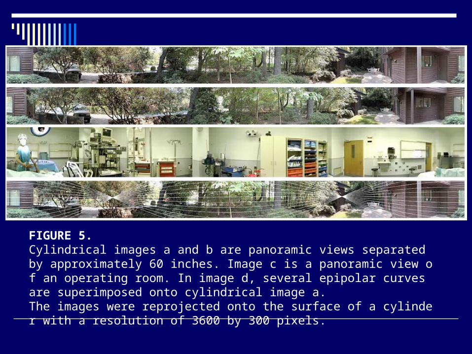
FIGURE 5. Cylindrical images a and b are panoramic views separated by approximately 60 inches. Image c is a panoramic view of an operating room. In image d, several epipolar curves are superimposed onto cylindrical image a.The images were reprojected onto the surface of a cylinder with a resolution of 3600 by 300 pixels.
Results
The epipolar geometry was computed by specifying 12 tiepoints on the front of the house.
As these tiepoints were added, we also refined the epipolar geometry and cylinder position estimates.
In Figure 5d, we show a cylindrical image with several epipolar curves superimposed.
After the disparity images are computed, they can be interactively warped to new viewing positions.

The following four images show various reconstructions.
Conclusions
Our methods allow efficient determination of visibility and real-time display of visually rich environments on conventional workstations without special purpose graphics acceleration.
The plenoptic approach to modeling and display will provide robust and high-fidelity models of environments based entirely on a set of reference projections.
The degree of realism will be determined by the resolution of the reference images rather than the number of primitives used in describing the scene.
The difficulty of producing realistic models of real environments will be greatly reduced by replacing geometry with images.