platforms and real options in large-scale engineering …
TRANSCRIPT

Platforms and Real Options in Large-Scale EngineeringSystems
by
Konstantinos Kalligeros
Dipl. Civil Engineering, National Technical University Athens, 2000S.M., Massachusetts Institute of Technology, 2002
Submitted to the Engineering Systems Divisionin partial fulfillment of the requirements for the degree of
Doctor of Philosophy
at the
MASSACHUSETTS INSTITUTE OF TECHNOLOGY
June 2006
c© Massachusetts Institute of Technology 2006. All rights reserved.
Author . . . . . . . . . . . . . . . . . . . . . . . . . . . . . . . . . . . . . . . . . . . . . . . . . . . . . . . . . . . . . . . . . . . . . . . . . . . .Engineering Systems Division
June 2006
Certified by. . . . . . . . . . . . . . . . . . . . . . . . . . . . . . . . . . . . . . . . . . . . . . . . . . . . . . . . . . . . . . . . . . . . . . . .Richard de Neufville
Professor, Engineering Systems DivisionThesis Supervisor
Certified by. . . . . . . . . . . . . . . . . . . . . . . . . . . . . . . . . . . . . . . . . . . . . . . . . . . . . . . . . . . . . . . . . . . . . . . .Olivier de Weck
Assistant Professor, Aeronautics & Astronautics and Engineering Systems
Certified by. . . . . . . . . . . . . . . . . . . . . . . . . . . . . . . . . . . . . . . . . . . . . . . . . . . . . . . . . . . . . . . . . . . . . . . .David Geltner
Director, Center for Real Estate,Professor of Real Estate Finance, Department of Urban Studies & Planning
Certified by. . . . . . . . . . . . . . . . . . . . . . . . . . . . . . . . . . . . . . . . . . . . . . . . . . . . . . . . . . . . . . . . . . . . . . . .Patrick Jaillet
Department Head & Edmund K. Turner Professor,Department of Civil and Environmental Engineering
Accepted by . . . . . . . . . . . . . . . . . . . . . . . . . . . . . . . . . . . . . . . . . . . . . . . . . . . . . . . . . . . . . . . . . . . . . . .Richard de Neufville
Chairman, Engineering Systems Division Education Committee
1

Platforms and Real Options in Large-Scale Engineering Systems
by
Konstantinos Kalligeros
Submitted to the Engineering Systems Divisionon June 2006, in partial fulfillment of the
requirements for the degree ofDoctor of Philosophy
Abstract
This thesis introduces a framework and two methodologies that enable engineering man-agement teams to assess the value of real options in programs of large-scale, partially stan-dardized systems implemented a few times over the medium term. This enables valuecreation through the balanced and complementary use of two seemingly competing designparadigms, i.e., standardization and design for flexibility.
The flexibility of a platform program is modeled as the developer’s ability to choosethe optimal extent of standardization between multiple projects at the time later projectsare designed, depending on how uncertainty unfolds. Along the lines of previous work,this thesis uses a two-step methodology for valuing this flexibility: screening of efficientstandardization strategies for future developments in a program of projects; and valuingthe flexibility to develop one of these alternatives.
The criterion for screening alternative future standardization strategies is the maximiza-tion of measurable standardization effects that do not depend on future uncertainties. Anovel methodology and algorithm, called “Invariant Design Rules” (IDR), is developed forthe exploration of alternative standardization opportunities, i.e., collections of componentsthat can be standardized among systems with different functional requirements.
A novel valuation process is introduced to value the developer’s real options to chooseamong these strategies later. The methodology is designed to overcome some presumedcontributors to the limited appeal of real options theory in engineering. Firstly, a graphicallanguage is introduced to communicate and map engineering decisions to real option struc-tures and equations. These equations are then solved using a generalized, simulation-basedmethodology that uses real-world probability dynamics and invokes equilibrium, rather thanno-arbitrage arguments for options pricing.
The intellectual and practical value of this thesis lies in operationalizing the identifi-cation and valuation of real options that can be created through standardization in pro-grams of large-scale systems. This work extends the platform design literature with IDR,a semi-quantitative tool for identifying standardization opportunities and platforms amongvariants with different functional requirements. The real options literature is extended witha methodology for mapping design and development decisions to structures of real options,and a simulation-based valuation algorithm designed to be close to current engineering prac-tice and correct from an economics perspective in certain cases. The application of thesemethodologies is illustrated in the preliminary design of a program of multi-billion dollarfloating production, storage and offloading (FPSO) vessels.
Thesis Supervisor: Richard de NeufvilleTitle: Professor, Engineering Systems Division

Olivier de WeckTitle: Assistant Professor, Aeronautics & Astronautics and Engineering Systems
David GeltnerTitle: Director, Center for Real Estate,Professor of Real Estate Finance, Department of Urban Studies & Planning
Patrick JailletTitle: Department Head & Edmund K. Turner Professor,Department of Civil and Environmental Engineering

to the “children:”
Johnny,
Kassandra,
Anna,
Irene,
Anastasia,
Ina and of course,
Konstantinos!

Acknowledgments
My deepest gratitude goes to my parents, Chryssanthos and Eirini, and my brother, Johnny,for the drive, love, unconditional support, and “good vibes” this effort required!
I ought to thank my advisor, Richard de Neufville, for steering me through and pushingme further than I thought I could go; Olivier de Weck, for his creative ideas, his care andfor being the catalyst that got the final stages of this thesis going; David Geltner, for hiscontagious open-mindedness, sharpness and enthusiasm; Patrick Jaillet for his observationsand suggestions that solidified some concepts in this thesis and broadened its audience.
I am deeply grateful to everyone who happened, or brought themselves to be at theright place at the right time over these years: Yiannis Anagnostakis, Yiannis Bertsatos
Alexandros, Lydia, Lenka and Susan. You have been the balancing factor during some veryunbalanced years. My special thanks to Iason and Andrea, who saw me through. Beth andTimea, you made a dull office, interesting and fun–thank you! I am also deeply thankfulto my family in the US, George and Margaret Carayannopoulos, and George and Jasmin
Lampadarios.Finally, many thanks to the sponsors of this work, who have provided insights, thoughts,
their experience and relevant data, particularly Adrian Luckins from BP and John Dahlgren
and Michele Steinbach from MITRE.

Contents
1 Introduction 19
1.1 Motivation . . . . . . . . . . . . . . . . . . . . . . . . . . . . . . . . . . . . 191.2 Platforms in consumer products and engineering systems . . . . . . . . . . . 191.3 Design for flexibility . . . . . . . . . . . . . . . . . . . . . . . . . . . . . . . 211.4 Platforms and flexibility . . . . . . . . . . . . . . . . . . . . . . . . . . . . . 231.5 Bridging the gap: thesis . . . . . . . . . . . . . . . . . . . . . . . . . . . . . 24
1.5.1 Approach . . . . . . . . . . . . . . . . . . . . . . . . . . . . . . . . . 241.5.2 Contributions . . . . . . . . . . . . . . . . . . . . . . . . . . . . . . . 25
1.6 Thesis outline . . . . . . . . . . . . . . . . . . . . . . . . . . . . . . . . . . . 26
2 Literature Review 27
2.1 Introduction . . . . . . . . . . . . . . . . . . . . . . . . . . . . . . . . . . . . 272.2 Product platforms and families . . . . . . . . . . . . . . . . . . . . . . . . . 282.3 Platform and standardization benefits . . . . . . . . . . . . . . . . . . . . . 30
2.3.1 Learning curve effects . . . . . . . . . . . . . . . . . . . . . . . . . . 302.3.2 Maintenance, Repair and operations benefits . . . . . . . . . . . . . 32
2.4 Platform selection and evaluation . . . . . . . . . . . . . . . . . . . . . . . . 342.4.1 Optimized search for platform strategies . . . . . . . . . . . . . . . . 362.4.2 Heuristic identification of platform strategies . . . . . . . . . . . . . 362.4.3 Product platform evaluation and design . . . . . . . . . . . . . . . . 37
2.5 Strategic view of platforms . . . . . . . . . . . . . . . . . . . . . . . . . . . 392.6 Flexibility and real options . . . . . . . . . . . . . . . . . . . . . . . . . . . 42
2.6.1 Flexibility and real options in engineering projects . . . . . . . . . . 452.6.2 Option valuation . . . . . . . . . . . . . . . . . . . . . . . . . . . . . 47
2.7 Summary and research contribution . . . . . . . . . . . . . . . . . . . . . . 53
3 Invariant Design Rules for platform identification 55
3.1 Introduction . . . . . . . . . . . . . . . . . . . . . . . . . . . . . . . . . . . . 553.2 Related work . . . . . . . . . . . . . . . . . . . . . . . . . . . . . . . . . . . 56
3.2.1 The design structure matrix (DSM) . . . . . . . . . . . . . . . . . . 573.3 Platform identification at the design variable level . . . . . . . . . . . . . . 60
7

3.3.1 sDSM system representation . . . . . . . . . . . . . . . . . . . . . . 603.3.2 Change propagation . . . . . . . . . . . . . . . . . . . . . . . . . . . 613.3.3 Platform identification . . . . . . . . . . . . . . . . . . . . . . . . . . 623.3.4 Algorithm for platform identification . . . . . . . . . . . . . . . . . . 64
3.4 Platform identification at higher system levels . . . . . . . . . . . . . . . . . 663.4.1 Activity SDSM representation . . . . . . . . . . . . . . . . . . . . . . 663.4.2 Exogenous parameters and change propagation . . . . . . . . . . . . 69
3.5 Exploration of platform strategies . . . . . . . . . . . . . . . . . . . . . . . . 703.5.1 Change absorbers and platform strategies . . . . . . . . . . . . . . . 71
3.6 Multi-level platforms . . . . . . . . . . . . . . . . . . . . . . . . . . . . . . . 743.7 Summary . . . . . . . . . . . . . . . . . . . . . . . . . . . . . . . . . . . . . 76
4 Flexibility valuation in large-scale engineering programs 79
4.1 Introduction . . . . . . . . . . . . . . . . . . . . . . . . . . . . . . . . . . . . 794.2 Design and development decisions . . . . . . . . . . . . . . . . . . . . . . . . 81
4.2.1 Assets and states . . . . . . . . . . . . . . . . . . . . . . . . . . . . . 824.2.2 Decisions on timing . . . . . . . . . . . . . . . . . . . . . . . . . . . 844.2.3 Decisions on target state . . . . . . . . . . . . . . . . . . . . . . . . . 864.2.4 Complex design and development structures . . . . . . . . . . . . . . 87
4.3 Valuation . . . . . . . . . . . . . . . . . . . . . . . . . . . . . . . . . . . . . 884.3.1 Calculation of conditional expectations . . . . . . . . . . . . . . . . . 914.3.2 Valuation of a reference design . . . . . . . . . . . . . . . . . . . . . 924.3.3 Valuation of two perfectly correlated states . . . . . . . . . . . . . . 934.3.4 Valuation of timing options . . . . . . . . . . . . . . . . . . . . . . . 954.3.5 Valuation of choice options . . . . . . . . . . . . . . . . . . . . . . . 96
4.4 Methodology performance and discussion . . . . . . . . . . . . . . . . . . . 964.4.1 Design decisions modeling . . . . . . . . . . . . . . . . . . . . . . . . 974.4.2 Algorithm Performance . . . . . . . . . . . . . . . . . . . . . . . . . 974.4.3 Valuation of uncorrelated states . . . . . . . . . . . . . . . . . . . . . 98
4.5 Summary . . . . . . . . . . . . . . . . . . . . . . . . . . . . . . . . . . . . . 103
5 FPSO program design study 105
5.1 Introduction . . . . . . . . . . . . . . . . . . . . . . . . . . . . . . . . . . . . 1055.1.1 FPSO process technology description . . . . . . . . . . . . . . . . . . 1075.1.2 FPSO program design case: problem statement and approach . . . . 108
5.2 Standardization effects . . . . . . . . . . . . . . . . . . . . . . . . . . . . . . 1145.2.1 Reduction in operating expenses . . . . . . . . . . . . . . . . . . . . 1155.2.2 Reduction in FEED cost and time . . . . . . . . . . . . . . . . . . . 1185.2.3 Reduction in construction cost . . . . . . . . . . . . . . . . . . . . . 1215.2.4 Reduction in construction time . . . . . . . . . . . . . . . . . . . . . 122
8

5.3 Screening of platform strategies . . . . . . . . . . . . . . . . . . . . . . . . . 1265.3.1 The low-hanging fruit . . . . . . . . . . . . . . . . . . . . . . . . . . 1265.3.2 Compromise strategies . . . . . . . . . . . . . . . . . . . . . . . . . . 126
5.4 Valuation of standardization program . . . . . . . . . . . . . . . . . . . . . 1295.4.1 Valuation results . . . . . . . . . . . . . . . . . . . . . . . . . . . . . 132
5.5 Summary . . . . . . . . . . . . . . . . . . . . . . . . . . . . . . . . . . . . . 134
6 Conclusions and future work 1376.1 Summary . . . . . . . . . . . . . . . . . . . . . . . . . . . . . . . . . . . . . 1376.2 Future research . . . . . . . . . . . . . . . . . . . . . . . . . . . . . . . . . . 138
6.2.1 Flexibility-based optimization and value created . . . . . . . . . . . 1396.2.2 IDR-based platform optimization . . . . . . . . . . . . . . . . . . . . 1396.2.3 Application: trading-off commitment and flexibility . . . . . . . . . 140
9

10

List of Figures
1-1 2-stage methodology for flexibility and platform design . . . . . . . . . . . . 24
2-1 Platform utilization among major automotive manufacturers . . . . . . . . 292-2 85% learning curve . . . . . . . . . . . . . . . . . . . . . . . . . . . . . . . . 322-3 Estimated inventory level savings due to standardization and demand pooling 352-4 Two-step process for designing platform variants . . . . . . . . . . . . . . . 382-5 Design for variety: spatial and temporal evolution of product families . . . 392-6 Flexibility in engineering, manufacturing and operations . . . . . . . . . . . 462-7 Two steps of a recombining binomial lattice of s . . . . . . . . . . . . . . . 482-8 Bin definition and transition probabilities in SSAP algorithm . . . . . . . . 52
3-1 DSM configurations that characterize physical links or information flows . . 583-2 Original and clustered DSM . . . . . . . . . . . . . . . . . . . . . . . . . . 583-3 Normalized SDSM, extended to include exogenous functional requirements . 613-4 Invariant Design Rules on an S-DSM . . . . . . . . . . . . . . . . . . . . . . 643-5 Clustering of a 45-variable DSM into 6 systems . . . . . . . . . . . . . . . . 673-6 DSM representation of design activities at a system level . . . . . . . . . . . 683-7 System-level DSM, extended to include functional requirements . . . . . . . 703-8 Invariant design rules for system-level DSM, given changes in FR1 . . . . . 713-9 Effect of removing the sensitivity of B to FR1 and F . . . . . . . . . . . . . 723-10 Effect of removing the sensitivity of A to B . . . . . . . . . . . . . . . . . . 723-11 Effect of removing the sensitivity of systems F and B to FR1 . . . . . . . . 733-12 Removing SDSM entries: simulation results . . . . . . . . . . . . . . . . . . 74
3-13 Decomposition of system A at the variable level . . . . . . . . . . . . . . . . 753-14 Decomposition of system A at the subsystem level . . . . . . . . . . . . . . 763-15 Re-partitioned SDSM, with platform that includes subsystem-level line items 76
4-1 An American timing option to obtain state w from state u: transition canoccur at any time within a time horizon. . . . . . . . . . . . . . . . . . . . . 85
4-2 A European option to obtain state w from state u: transition can occur onlyat a specific time. . . . . . . . . . . . . . . . . . . . . . . . . . . . . . . . . . 85
4-3 An American option with time-to-build ttb . . . . . . . . . . . . . . . . . . . 86
11
4-4 Choice between development options to 4- and 5-level garage . . . . . . . . 874-5 A complex structure of development decisions . . . . . . . . . . . . . . . . . 884-6 Characterization of the proposed option valuation methodology (shaded boxes)
and comparison with other valuation approaches. . . . . . . . . . . . . . . . 904-7 Two-dimensional bin definition and some representative values at time t . . 914-8 Inferred price of risk from reference design valuation . . . . . . . . . . . . . 934-9 Risk and discount rate for design w . . . . . . . . . . . . . . . . . . . . . . . 944-10 American call option: Valuation errors . . . . . . . . . . . . . . . . . . . . . 994-11 American call option: Valuation errors . . . . . . . . . . . . . . . . . . . . . 1004-12 American call option: Valuation errors . . . . . . . . . . . . . . . . . . . . . 1014-13 American call option: Valuation errors . . . . . . . . . . . . . . . . . . . . . 102
5-1 Greater Plutonio FPSO offshore Angola (operated by BP) . . . . . . . . . . 1065-2 Main topsides facilities functions and equipment (simplified) . . . . . . . . . 1085-3 Comparison between assumed functional requirements of FPSOs α and β . 1115-4 FPSOs α and β program development decisions . . . . . . . . . . . . . . . . 1135-5 Effects of system standardization between FPSOs α and β . . . . . . . . . . 1155-6 Assumed percent breakdown of development costs by system, FPSO α . . . 1165-7 FEED cost and time as a function of standardization by weight . . . . . . . 1195-8 Assumed learning curves in FPSO construction costs . . . . . . . . . . . . . 1225-9 FPSO α construction schedule. All links are start-to-start with lag. . . . . . 1255-10 Original SDSM for FPSO α . . . . . . . . . . . . . . . . . . . . . . . . . . . 1275-11 Partitioned SDSM for FPSO α, showing standardized systems according to
strategy 0 (no entries removed). . . . . . . . . . . . . . . . . . . . . . . . . . 1275-12 Pareto-optimal strategies . . . . . . . . . . . . . . . . . . . . . . . . . . . . 1295-13 FPSOs α and β program development decisions . . . . . . . . . . . . . . . . 130
12

List of Tables
313.1 DSM types, applications and analysis techniques . . . . . . . . . . . . . . . 593.2 Algorithm for the partitioning of standardized DSM items . . . . . . . . . . 65
5.1 Main FPSO process systems and utilities . . . . . . . . . . . . . . . . . . . 1095.2 Assumed functional requirements for FPSO α and β . . . . . . . . . . . . . 1105.3 Assumed FPSO annual spare part costs for each system ($1,000) . . . . . . 1175.4 Assumed FPSO FEED costs for each system ($1,000) . . . . . . . . . . . . 1205.5 Assumed FPSO α construction costs for each system ($1,000) . . . . . . . . 1235.6 Assumed FPSO β construction costs for each system ($1,000) . . . . . . . . 1245.7 Measurable standardization effects: g(%) functions for β1 . . . β16 . . . . . . . 1305.8 Standardization strategies . . . . . . . . . . . . . . . . . . . . . . . . . . . . 1315.9 Estimated costs for 5 selected standardization programs (based on current
prices of oil, gas and steel). . . . . . . . . . . . . . . . . . . . . . . . . . . . 1325.10 Value of states αβi . . . . . . . . . . . . . . . . . . . . . . . . . . . . . . . . 1335.11 Value of construction options for states αβi . . . . . . . . . . . . . . . . . . 1335.12 Option to design and develop states αβi . . . . . . . . . . . . . . . . . . . . 134
13

14

Nomenclature
at(m) Total number of paths falling in bin m at time t
bt(m,n) Total number of paths falling in bin m at time t and bin n at t + δt
c The opportunity FEED cost of standardization, i.e., the cost difference be-tween a fully customized and a fully standardized design, over the differencein FEED time.
c′ The opportunity construction design cost of standardization, i.e., the costdifference between a fully customized and a fully standardized design, overthe difference in detailed design time.
Cαβ Time-to-build FPSO β, given that FPSO α is already builtCβ0 Time-to-build a completely customized FPSO β0
Cuw “Construction” cost for obtaining state w from state u
CAP gasα Oil production capacity of FPSO α (mbod)
CAP oilα Gas production capacity of FPSO α (mmscfd)
CEQ[·] The certainty-equivalent of a quantity, i.e., the expected quantity reducedby a dollar risk premium and then discounted at the risk free rate.
CF (xα, st) ≡ CFα(st) The cash flows that would be generated by FPSO α individually(in the absence of FPSO β) per time period, given state of uncertain factorsst
CF fixα (s) Fixed production costs for FPSO α
CF varα (s) Variable production costs for FPSO α
CFαβ(st) The cash flow generated by the simultaneous operation of FPSOs α and β
per time period, given state of uncertain factors st
Dαβ Ch.5: cost to design FPSO β, given that FPSO α is already designed andconstructed
Dβ0 Ch.5: cost to design an entirely customized FPSO β0
Duw “Design” cost for obtaining timing option to state w from state u
Fuw Value of timing option to obtain state w in exchange of state u
FR Vector of functional requirementsg1(xα,xβ) % reduction in fixed production costs for simultaneous operation of FPSOs
α and β
15

g2(xα,xβ) % reduction in front-end-engineering design (FEED) cost of FPSO β, giventhat FPSO α is already designed
g3(xα,xβ) % reduction in front-end-engineering design (FEED) time of FPSO β, giventhat FPSO α is already designed
g4(xα,xβ) % reduction in construction and fabrication cost of FPSO β, given thatFPSO α is already constructed
g5(xα,xβ) % reduction in construction and fabrication schedule time of FPSO β, giventhat FPSO α is already constructed
h Index for alternative underlying assets (choices) in a choice option. E.g.,corresponds to alternative FPSO designs β1 . . . βh in Ch. 5.
Huw The holding value of an option to obtain w by giving up u
Iuw Value of immediate exercise of an option to obtain w by giving up u
j Ch. 3: indexCh. 4: indicator for time period
J Ch. 3: Jacobian matrixCh. 4: Total number of time instances in a simulation (including t = 0)
k Ch. 3: step in IDR algorithmCh. 4: indicator for a simulation event (path)
K Total number of simulation events (paths)M Total number of bins per time period in a simulationm,n Indices for bins, m typically corresponding to time t and n to time t + δt
mbd Thousand Barrels per Day, common unit in oil productionmbod Thousand Barrels of Oil per Day, common unit in oil productionmmscf Million Standard Cubic Feet, common unit of gas volume in oil productionmmscfd Million Standard Cubic Feet per Day, common unit of gas productivity in
oil productionN Total number of sources of uncertainty in a simulationp, 1− p Real-world probabilitiesPt(m,n) m,n element of transition probability matrix at time t, real-world dynamicsq, 1− q Risk-neutral probabilitiesrf Continuously-compounded risk-free rateru Continuously-compounded rate, risk adjusted to appropriately discount ex-
pected values of state or option u
RPα Risk premium demanded by investors holding asset α
st Value of vector of uncertain factors at time t
smt representative value of vector of uncertainties at time t in bin m
16

sd Ch. 2: in a binomial lattice, the “down” value of the underlying asset oneperiod in the future
sgast Spot price of oil ($/bbl) at time t
soilt Spot price of gas ($/mscf) at time t
sstlt Spot price of steel ($/ton) at time t
su Ch. 2: in a binomial lattice, the “up” value of the underlying asset oneperiod in the future
t TimeT Time, generally used to denote terminal time, time of option expiration, or
the time horizonTDD
βα Detailed (construction) design time required for an FPSO β partially stan-dardized based on FPSO α
TDDβ0
Detailed (construction) design time required for a fully customized FPSO β0
TtBi Time-to-build asset i, the time lag between the decision to exercise an optionand obtaining the asset
TtDi Time-to-design asset i, the time lag between the decision to exercise a choiceoption and obtaining the asset or the corresponding construction option
TtDαβ Time-to-design FPSO β, given that FPSO α is already designedTtDβ0 Time-to-design a completely customized FPSO β0
x Vector of design variables (or system line items) in SDSMx∗ Vector of design variables (or system line items) of variant ∗xα Vector of design variables (or system line items) of variant α
xαc Subset of the design vector of variant α that is unique to that variant
xp Subset of the design vector that is equal for two variants and constitutes theplatform between them
V3b(α1) Ch. 5: it is the value, calculated using approach 3b, of an FPSO α that hasbeen optimized using approach 1 (see page 109).
Vu Total value of state u, including the value of any associated optionsV cf
u Intrinsic value of state u, i.e., the discounted expected value of future cashflows
α Ch. 3: the name of one system variant;Ch. 5: the name of the first FPSO in a development program
αβ1 . . . αβ68 Names of the states of simultaneous operation of FPSOs α and β1 to β68
respectively.β0 The name of a fully customized FPSO β
β1 . . . β68 Ch. 3: names of system variants;
17
Ch. 4: the name of the second FPSO in a development program∆C(xα,xβ) The construction and fabrication cost difference between customizing all
systems in FPSO β, minus the (reduced) cost of re-using the designs fromFPSO α.
∆D(xα,xβ) The FEED cost difference between customizing all systems in FPSO β, minusthe (reduced) cost of re-using the designs from FPSO α.
δt Time increment used for computationsκ Number of line items (design variables or systems) in SDSMλ Price of riskξ Number of external functional requirements in SDSMΠk Running subset of SDSM line items in iteration k of the IDR algorithm
18

Chapter 1
Introduction
1.1 Motivation
The work in this thesis is motivated by a gap between two seemingly competing but relatedconcepts in the academic literature and practice. The first is platform design, especiallyfor large-scale engineering systems. The second is design for flexibility, an emerging trendin practice and a hot topic of academic research over the past years. Based on intuitionalone, design for flexibility and platform design seem competing paradigms: a platform is,after all, a set of standardized components, processes, technology etc. among a family ofproducts, that is usually expensive to design and develop, and constrains the developmentof new products and the marginal improvement of existing ones. The counter-argument isthat platforms enable the development of (possibly very different) variants at low cost; inthis sense, a platform is a springboard for entering markets for new products or expandingexisting product families: it is almost synonymous with having flexibility to introduce morenew products, faster! Apparently, there is no intuitive and conclusive answer as to whetherdesign for flexibility and platform design are competing paradigms.
In fact, the hypothesis for this work is that platform design creates and destroys futureflexibility at the same time and in different ways. The two paradigms can be competingin some ways and complementary in others. Therefore, there is a need for a structuredprocess for concurrent platform design and flexibility design. This need is driven by thehigh potential value of both platforms and flexibility. For many systems the stakes are nottrivial, as shown by direct data as well as industry trends.
1.2 Platforms in consumer products and engineering systems
A quick look into the firms that lead their industry sector reveals that they have movedfrom producing a single product in large quantities, to differentiating the performance char-acteristics of their product range. Such trends were seen in consumer products, such aswalkmans and electric appliances, as well high-technology complex systems such as com-
19

mercial aircraft. The shift in the design paradigm from one-at-a-time designs to “masscustomization” (i.e., very different products variants that share a common platform) hasenabled organizations to tap into economies of scale, knowledge sharing, easier developmentof a larger number of variants, maintenance benefits and spare part reduction (enjoyed byboth manufacturers and users of product variants).
Examples are abundant. In the 1980s, Sony based hundreds of variants of the theWalkman on just three platforms for the mechanical and electronic parts of the product(Sanderson 1995). Also maintaining “hidden” components similar, Black and Decker builta line of products with various power requirements based on a single scalable electric drive(Meyer & Lehnerd 1997). At the same time, Airbus was able to differentiate significantlyin the performance characteristics of a series of aircraft (particularly A318, A319, A320and A321), while retaining the same “look and feel” in the cockpit, thereby reducing crewtraining time and creating value for its clients. This way, Airbus extended the concept ofplatforms beyond the common design of physical components. Platforms can also implycommon intangible characteristics that add value to a family of products.
Even oil companies have been unlikely followers of the platform design paradigm. For ex-ample, some recent programs of oil development projects have been developed according toa complete standardization strategy. Exxon/Mobil’s Kizomba A and Kizomba B platformsoffshore Angola are built almost entirely on the same identical design. BP’s development inthe Caspian Sea offshore Baku, Azerbaijan, consisted of 6 almost identical semi-submersiblerigs. The three trains at BP’s Atlantic Liquefied Natural Gas (LNG) plant were designedidentically and constructed sequentially.
In consumer products, the platform design paradigm is ubiquitous because of clear andwell-documented benefits. Given a high volume (or expected volume) of production of aproduct family, developers expected to share the learning curve for the design and man-ufacturing of platform components among all variants. The cost of redesigning platformcomponents for every variant is also avoided, thereby leveraging capital expenses of produc-ing variants and the initial platform. Significant benefits are also experienced in the formof strategic supplier agreements and alliances, resulting in fast and reliable supply chains.Overall, platform design has enabled product families with very similar functional charac-teristics to suit customers’ needs exactly, thereby expanding and re-inventing markets, andgiving developers competitive advantage.
Platform benefits are also documented in the development of large-scale systems, e.g., oilexploration and production infrastructure (McGill & de Neufville 2005). Standardization ofcomponents and processes in such projects has resulted in double-digit percentage reductionsin capital costs, cycle time, operability and maintainability. Besides leveraging direct andindirect engineering costs, repeated upstream developments have shown learning curves andsavings in fabrication costs. Repeated supplier agreements and larger material orders havecontributed to lower contract costs and less risky contract deliveries. The re-use of identicalsystems and components across projects and the common design philosophy overall, has
20

resulted in lower spares inventories, personnel training expenses and operational processdesign. Finally, the approach has resulted in better utilization of scarce engineering andmanagement personnel capable of projects of such scale. Being committed to utilizinglocal human resources, oil companies re-using designs and implementing platforms havealso experienced a steep learning curve in local capability. Seemingly, platform benefits aredirectly transferrable to large-scale systems.
The next intellectual challenge for platform strategists and academics lies in the design,development and utilization of platforms in time, in a dynamic setting of changing customerpreferences, cost line items, product value and evolving technology. A platform strategy,i.e., the selection and extent of platform components, must not only satisfy static or de-terministically changing criteria of optimality; it must enable the evolution and adaptationof the entire organization to changing conditions as the future unfolds. Fricke & Schultz(2005) report the main challenges with implementing platform strategies and architectures:
• The incorporation of elements in system architectures that enable them to be changedeasily and rapidly.
• The intelligent incorporation of the ability to be insensitive or adaptable towardschanging environments.
1.3 Design for flexibility
What Fricke & Schultz (2005) call the next challenge in platform design is that it incor-porates flexibility. It can be argued that flexibility is not just an opportunity for addedvalue or a welcome side-effect of a good design; in a competitive environment, it is a designrequirement. In the words of Kulatilaka (1994),
A myopic policy does not necessarily fail; it fails insofar as uncertainty represents
opportunity in a competitive environment.
For example, de Weck, et al. (2003) point out that much of the financial failure of bothcommunication satellite networks built in the mid-nineties, Iridium and Globalstar, couldhave been avoided if the systems were designed to be deployed in stages, thereby retainingthe programmatic flexibility to change the scale of the project, its configuration and datatransmitting capacity before its completion1. In real estate, volatile markets have alsogiven rise to flexible development. Archambeault (2002) reports the rapid decline in value
1Iridium and Globalstar were two similar, competing systems of satellite mobile telephony. During the
time between their conception, licencing, design and deployment, a total of about 8 years, GSM networks,
a competing terrestrial technology, had come to dominate many of the core markets these systems were
targeting. Despite the enormous technical success of these systems, both companies filed for bankruptcy
protection with losses between $3-5bn each. At this time, the two satellite networks operate significantly
under capacity with clients such as the US government, exploiting their technical niche of global coverage
that terrestrial cellular networks cannot provide.
21

for telecommunications hotels after the dot-com market crash at the turn of the century2.With the dot-com market crash, the vacancy rate of these buildings increased steeply andtheir owners started to look into their reconfiguration capability. Those buildings that weredesigned to cheaply convert to laboratory or office space did so at low costs; others had tobe drastically re-designed. Similar cases in real estate can be found in Greden & Glicksman(2004).
Despite the strong case for considering flexibility in design, most engineering managersstill focus on “point designs.” Cullimore (2001) summarizes the current “point-design”engineering paradigm, and contrasts it with an approach that accounts for uncertainty andflexibility:
Point designs represent not what an engineer needs to accomplish, but rather
what is convenient to solve numerically assuming inputs are known precisely.
Specifically, point design evaluation is merely a subprocess of what an engineer
must do to produce a useful and efficient design. Sizing, selecting, and locating
components and coping with uncertainties and variations are the real tasks.
Point design simulations alone cannot produce effective designs, they can only
verify deterministic instances of them.
Wang & de Neufville (2005), Wang (2005) and de Neufville (2003) built on the conceptand theory of real options to distinguish between managerial flexibility that is emergentor coincidental in the development and operation of a system, and flexibility that has tobe anticipated, designed and engineered into systems. They call the former, “real options‘on’ projects” and the latter, “real options ‘in’ projects.” Several academic papers haveexplored case studies of options “in” projects: de Weck et al. (2003) suggested alternativeprogrammatic and technical design for the Iridium and Globalstar systems so that flexibilitywas created through staged deployment; Kalligeros & de Weck (2004) explored the optimalmodularization of an office building that would be required to contract and change use in thefuture; Wang (2005) used mixed-integer stochastic programming to value path-dependentoptions in river basin development; Markish & Willcox (2003) explore the coupling betweentechnical design and programmatic decisions as they provide flexibility in the deploymentof a new family of aircraft; Zhao & Tseng (2003) investigate the flexible design of a simplebuilding, a parking garage with enhanced foundations and columns, that can be expandedto cover local parking demand.
However, flexibility design and real options “in” systems are still very far from becom-ing current practice. Despite the appeal that these case studies have to their respectiveengineering audiences, neither the concept nor the methodology has so far had a significant
2Telecommunications hotels are buildings specially configured to host electronic equipment (servers, stor-
age etc.), servicing the computational needs of internet companies. The design requirements for such build-
ings are very different from residential or office construction: ceilings can be low, HVAC requirements are
stringent, natural light is avoided, and there is very little need for parking.
22

impact in the way systems are designed and developed. We can begin to postulate aboutthe reasons this is so:
• The examples in the academic literature can often be perceived to be contrived, unre-alistic and over-simplified in order to facilitate analysis. This way they lose potentialfor real impact and fuel practitioners’ resistance.
• The organizational and incentive structure between the entities that conceive, design,sanction, finance and execute projects is often such that the involved teams are notinclined to pursue the creation of flexible systems. This is often because the costsof engineering flexibility must be justified internally by teams different than the onesthat are attributed the added value. As a result, the research efforts of academicshave no audience in the industry, to own and promote new results.
• Even if the incentive and will to design flexibility in engineering systems exists, thereis no technical guidance as to how. In other words, there is a lack of an unambiguouslanguage for modeling design and development decisions as real options.
• Currently, real option valuation technology relies too heavily on its financial optionvaluation counterpart. As a result, both concept and practice appear restrictive,counter-intuitive and difficult to understand by engineering practitioners in the cul-tural context of real organizations.
1.4 Platforms and flexibility
On one hand, platform design and standardization appears to be a great source of value.On the other, flexible design was demonstrated to be almost a necessity in an uncertaincompetitive environment. To what extent are these paradigms competing and how mightthey be complementary, especially for the development of large-scale systems?
They can be complementary because standardization can increase strategic flexibilityby enabling the developer to design and construct faster and more reliable systems, useexisting expertise to enter new ventures and markets cheaply, or even exit projects retain-ing high salvage value (because systems and components can be used in other projects).As such, platforms are equivalent to “springboards,” bringing the organization closer tonew ventures. Platforms are also the source of operational flexibility, because they enablethe inter-changeability of components and modules. This is ubiquitous, e.g., in personalcomputers and electronics with standardized interfaces.
However, platform design can be detrimental to strategic flexibility, especially in thelong run. Extensive standardization can be blamed for (risky) locking-in with suppliers andtechnology, limiting innovation and creativity within the organization. An equally real riskconcerns the extensive design of inflexible platforms that cannot accommodate changingfuture requirements.
23

It is evident that optimal standardization decisions must include flexibility consider-ations, and conversely, that flexible designs can be implemented through component andprocess standardization when multiple instances or variants of a system are involved. Theevaluation of programs of large-scale systems with considerations for platforms and flexibil-ity is a new paradigm in system design.
1.5 Bridging the gap: thesis
This thesis introduces a framework and two methodologies that enable engineering manage-ment teams to assess the value of flexibility in programs of large-scale, partially standardizedsystems implemented a few times over the medium term.
1.5.1 Approach
The proposed framework is presented in the context of a development program with twophases, i.e., two assets designed and constructed sequentially. These can be partially basedon the same platform, i.e., share the design of some of their components and systems. Itis assumed that the decision to standardize certain components between the two systems istaken at the time the second asset is designed, and that different standardization strategies(i.e., selection of common components) will be followed depending on information aboutthe state of the world at that time. The value of the program at the first stage includes thevalue of flexibility to optimally design and develop the second development, based on the“design standard” or platform established with the first.
This work provides a two-step methodology for valuing the first-stage design, as shownin Figure 1-1. The first step involves screening alternative standardization strategies for thesecond development. The second step involves valuing the flexibility to choose among thesestandardization strategies for the second-phase development. This flexibility is associatedwith the first-phase system and is an intrinsic part of its value.
Figure 1-1: 2-stage methodology for flexibility and platform design
24

Screening of standardization opportunities is based on a novel methodology and algo-rithm for locating collections of components that can be standardized among system vari-ants, given their different functional requirements. The criterion for screening alternativefuture standardization strategies is the maximization of measurable standardization effectsthat do not depend on future uncertainties. Examples of such criteria may be reduction instructural weight or construction time reduction for later projects. Using multi-disciplinaryengineering judgment and simulation, the methodology locates standardization strategiesthat optimize these criteria, e.g., finds standardization strategies that are Pareto-optimalin reducing construction time and structural weight.
The program’s flexibility is the ability to choose from these standardization strategieslater, depending on how uncertainty unfolds. Because the screened designs are Pareto-optimal in maximizing effects that do not depend on uncertainty, the choice of one ofthese designs will be optimal in the future. For example, assume two potential designs forthe second asset, one minimizing structural weight and the other minimizing constructioncycle time. If these designs are Pareto-optimal, then one cannot obtain a weight reductionwithout increasing cycle time. In the future, the weight-minimizing design might be chosenif the price of construction material is high and the price of the output products is low; thefaster-to-build design will be chosen if the reverse conditions prevail. Whilst it is not knowna-priori which design will be chosen (because the future prices of construction material andoutputs are unknown), it is sure that it will be one of the Pareto-optimal designs.
The flexibility to choose the design and development timing of the second asset in thefuture is inherent to the value of the entire program. Moreover, if the designer of the firstasset is able to influence the flexibility available to the designer of the second asset, thenthere is an opportunity for value creation. This is the value of flexibility engineers candesign into engineering systems through standardization.
1.5.2 Contributions
The intellectual and practical value of this thesis lies in operationalizing the concepts de-scribed above; i.e., providing a structured and systematic process that enables the explo-ration of platform design opportunities and flexibility for programs of large-scale systems.Platform design in large-scale projects is inherently a multi-disciplinary effort, subject tomultiple uncertainties and qualitative and quantitative external inputs. To the best of theauthor’s knowledge, no such design management methodology exists to date, that is (a)suitable for large-scale, complex projects; (b) modular, with modules that are based ontried and tested methods or practices; (c) open to inter-disciplinary and qualitative expertopinion; (d) effectively a basis for communication between the traditionally distinct disci-plines of engineering and finance. Each of the two steps in the proposed methodology is anovel contribution.
25

Invariant Design Rules This is a novel methodology and algorithm for the explorationof standardization opportunities at multiple levels of system aggregation, among variantswithin a program of developments. The Invariant Design Rules are sets of componentswhose design specifications are made insensitive to changes in the projects’ functional re-quirements, so that they can be standardized and provide “rules” for the design of cus-tomized components. The IDR methodology uses Sensitivity Design Structure Matrices(SDSM) to represent change propagation through the system and a novel algorithm forseparating customized systems and invariant design rules.
Engineering flexibility valuation The program’s flexibility is the ability to choose fromthese standardization strategies later, depending on how uncertainty unfolds. For the en-tire methodology to have impact, the valuation of this flexibility must be performed in anengineering context. With this rationale, a novel real option valuation process is developed,that overcomes some presumed contributors to real options analysis’ limited appeal in engi-neering. The proposed methodology deviates very little from current “sensitivity analysis,”practices in design evaluation. Firstly, a graphical language is introduced to communicateand map engineering decisions to real option structures and equations. These equations arethen solved using a generalized, simulation-based methodology that uses real-world prob-ability dynamics and invokes equilibrium, rather than no-arbitrage arguments for optionspricing.
The real options valuation algorithm can appeal to the engineering community becauseit is designed to overcome the barriers met by most real option approaches to design so far.At the same time, the algorithm is correct from a diversified investor’s perspective undercertain conditions.
1.6 Thesis outline
Chapter 2 provides a brief literature review of the basic modules of this thesis: platformdesign and development, standardization benefits in engineering and manufacturing, flexi-bility design and real options. Chapter 3 develops the Invariant Design Rules methodologyand algorithm in detail. Chapter 4 explains the real option valuation methodology, andpresents preliminary results compared to published benchmarks. Chapter 5 brings togetherthese methodologies, in a case study on standardization between multi-billion dollar Float-ing Production, Storage and Offloading (FPSO) units for oil production. A final chaptersummarizes the thesis and proposes directions for future research.
26

Chapter 2
Literature Review
2.1 Introduction
This chapter provides the intellectual support for the thesis as documented in the academicand practical literature. As the problem statement is multi-disciplinary, so is the body ofknowledge that supports this work. Section 2.2 begins with an account of platforms. Inthe product design literature, a primary problem is to design a set of components that iscommon between variants in such a way as to maximize the value of the entire productfamily. Recent contributions in this field show that uncertainty in the specifications offuture variants should be a driver for the design of the initial platforms. Specifically, somerecent literature is based on the hypothesis that real option value should be the objectivefor platform design decisions; by including real option value in the objective function it ispossible to account for the organization’s flexibility to release new products on the basis ofexisting platforms. Similar ideas are also found in the management strategy literature todescribe organizations and their evolution through time. In this sense, a platform representsall the core capabilities of an organization, not just physical infrastructure, that enables theorganization to evolve, so the word “platform” is often used to mean “springboard.” Justas physical product platforms enable the release of new products, core capabilities enablethe evolution of organizations.
The flexibility to evolve, be it a product family or an entire organization, has been con-ceptualized as a portfolio of real options. These real options can be valued using contingentclaims analysis, a methodology for modeling and quantifying flexibility, that is based on adeeply mathematical theory in finance and economics. Section 2.6 summarizes the basics ofoptions theory, some applications in valuing managerial flexibility and how it can be appliedto flexibility in real systems.
The chapter concludes with a research gap analysis. As described in Chapter 1, thisresearch provides two engineering management tools that extend the respective literaturestrands. A proposed technical methodology for screening dominant standardization oppor-tunities among system variants extends the platform design literature. The real options
27

literature, particularly in the context of engineering design, is extended with a method-ology for mapping design and development decisions to structures of real options, and asimulation-based valuation algorithm designed to be close to current engineering practiceand correct from an economics perspective.
2.2 Product platforms and families
“A platform is the common components, interfaces and processes within a product family”(Meyer & Lehnerd 1997). The development of platform-based product families involves thestandardization of certain components and their interfaces with the non-standardized com-ponents. More generally, a platform strategy involves all the engineering and managementdecisions on how, when and what product variants and platforms to develop.
At the extreme, a platform strategy involves the standardization of most of a product’scomponents: it is the paradigm set by Henry Ford. At the other extreme, the customizationof a product can rely on the customization of all of its components, which is the casewith integral, as opposed to modular, products. An intermediate solution is enabled withthe partial customization of components within a family of products; the part that is notcustomized is the platform for that product family. Firms, particularly in the automotiveindustry, are leading the field in developing extremely customized products based on verysmall numbers of product families. Consumer products and electronics are also often basedon few platforms, whilst offering a great variety of functional characteristics to the end user;e.g., see Simpson (2004), Meyer & Lehnerd (1997) for case studies on Black and Decker’selectric motor platform for power tools. In achieving “mass customization,” as this trendis often called, firms have to balance the tradeoffs between developing too many and toofew variants on a single platform. Figure 2-1 shows the average number of vehicle variantsbased on a single platform for 5 major automobile manufacturers (current and projected).Even though there is a clear trend to base more variants on a single platform, there alsoseems to be an “optimum equilibrium” which changes over time. For example, Toyota seemto plan to base 5 variants off of a single platform on average by 2006, from 4 in 2004;Honda is shown to go from 2 to 3 in the same time frame. This reflects a balance betweenthe benefits and costs of developing product families, which depend both on static factors,evolving technology and a changing dynamic marketplace.
On the upside, platform design leads to common manufacturing processes, technology,knowledge transfer across the organization and its supply chain and reduction in manufac-turing assets and tooling. From an organizational viewpoint, a product platform enablesthe firm to have a cross-functional team within product development; this in turn makesproduct and process integration much easier and less risky. In a more dynamic context,platform design enables the manufacturing organization to delay the so-called “point of dif-ferentiation:” this is the first instance in time that (a) the design and (b) the fabrication oftwo products in the same family begins to differ. Delayed differentiation (or postponement,
28

Figure 2-1: Platform utilization among major automotive manufacturers (Suh 2005)
as it is referred to in the supply chain literature) enables just-in-time production and fasterreactions to fluctuating demand. According to Ward, et al. (1995), delayed differentiationin design is a key driver of Toyota’s excellence in development time and quality. In short,platforms in manufacturing lead to lower design and production costs, higher productivity innew product development, reduction in lead times, and increased manufacturing flexibility.
On the other hand, basing a range of products on a platform can have disadvantages. Inthe short term, the initial cost of developing a platform is often much higher than the costof designing and producing a single product (Ulrich & Eppinger 1999). This cost increaseis accompanied by an increase in technical risks: since many product variants are basedon the same platform, the likelihood and impact of technical errors in the design of theplatform is larger. Furthermore, sharing too many components may reduce the perceiveddifferentiation between products in a family. This was reported to be the case with theautomobile brands belonging to Volkswagen, which were perceived by the public to be toosimilar to justify their price differences. Furthermore, in the long term platform design mayincrease an organization’s risk exposure: the platform development cost has to be recoupedfrom savings that depend largely on the number of variants produced and the productionvolume for each one. The increased risk in platform development arises because of theuncertainty regarding future demand for the variants. Finally, by developing platforms,organizations inadvertently lock in to the platform’s technology, architecture and supplychain; after all, this is exactly the source of production cost reductions. Locking in for thelong-term however, reduces the organization’s ability to evolve.
Because of these benefits and costs associated with a platform strategy, there is extensiveliterature on the optimization of a platform and a family of products. Jose & Tollenaere(2005) write: “the selection of a platform requires a comprehensive balance of the number
of special modules versus the number of common modules.”
29

To address this question, the platform design literature has encountered two main chal-lenges: firstly, the organization of a complex system into modules and the identification of acommon module (platform) in the product family. The second area of research has been toquantify the benefits arising from a platform strategy. For fairly simple systems, platformidentification and family design optimization have been integrated in a single optimizationframework. For an extensive review of the current literature on product platform design seeSimpson (2004), Simpson, et al. (2006) and Jose & Tollenaere (2005). Section 2.3 provides abrief account of the benefits of platform design in design and manufacturing as documentedin the literature over many years. Section 2.4 summarizes recent progress in modeling thesebenefits in platform evaluation and selection methods.
2.3 Platform and standardization benefits
Some of the platform benefits experienced in the automotive industry were described brieflyabove. A comprehensive account of the benefits organizations should consider before movingto a platform design strategy, including quantifiable as well as “soft” criteria, is given inSimpson, et al. (2005). Regarding the portfolio of platformed products as a whole, platformbenefits include increased customer satisfaction, product variety, organizational alignment,upgrade flexibility, reliability and service benefits, change flexibility, ease of assembly andothers.
In this section the focus is on the platform benefits experienced by design and manu-facturing organizations of larger-scale systems that are produced in smaller quantities thanconsumer products, e.g., airplanes, ships or infrastructure. Important standardization ben-efits for these classes of products, that are usually overlooked in consumer products, arelearning curve effects and spare part inventory management efficiencies.
2.3.1 Learning curve effects
Learning curves, generally experience curves, were first systematically observed and quan-tified at the Wright-Patterson Air Force Base in the United States in 1936 (Wright 1936).It was determined that manufacturing labor time decreased by 10-15% for every doublingof aircraft production. The scope of the effect was extended in the late 1960’s and early1970’s by Bruce Henderson at the Boston Consulting Group (Henderson 1972). “Experiencecurves,” as the extended concept is called, includes more improvements than cycle time,e.g., production cost, materials, administrative expenses, distribution cost savings etc.
Interestingly, the quantification of these effects reveals that the percent improvementis constant as the number of repetitions (i.e., production volume) increases. A commonlyused model for learning curves is based on power laws, i.e.,
yx = y1xz
30

where yx represents production time (or cost) needed to produce the x’th unit of a series;z = ln b/ ln 2; and b is the constant learning curve factor. Typical learning curve factors areshown in Table 2.1.
Table 2.1: Typical learning curve factors (NASA 2005)
Industry b
Aerospace 85%
Shipbuilding 80-85%
Complex machine tools for new models 75-85%
Repetitive electronics manufacturing 90-95%
Repetitive machining or punch-press operations 90-95%
Repetitive electrical operations 75-85%
Repetitive welding operations 90%
Raw materials 93-96 %
Purchased Parts 85-88 %
The major contributors and justification for experience curves are found in the physicalconstruction and manufacturing processes. Repetition causes fewer mistakes, encouragesmore confidence and less hesitation among workers. Production processes become stan-dardized and more efficient, making better use of equipment and allocation of resources.In a well-managed supply chain, these benefits are experienced by suppliers and reflectedas the cost and time savings in the value of the final product; see Goldberg & Tow (2003),Ghemawat (1985), and Day & Montgomery (1983).
The same causes of experience curves are seen in industries of large scale systems imple-mented few times over the medium term. In the oil industry, repeat engineering and con-struction has been observed to have three major effects: firstly, capital expense (CAPEX)reduction, mainly due to repeat engineering and contracts with preferred suppliers. Sec-ondly, value is created due to reduced operating expenses (OPEX) for the second andsubsequent projects. This is mainly due to reduced risk in start-up efficiency, improveduptime, and commonality of spares and operator training. Finally, project engineers andmanagers use proven designs and commissioned interfaces without “re-inventing the wheel.”Standardization implies reduced front-end engineering design (FEED) effort requirements,fewer mistakes, increased productivity, learning etc., which in turn imply reduced cycle time.This can be extremely valuable by accelerating the receipt of cash flows from operations,thus increasing their value. Given a growing concern in the oil industry about the availabil-ity of trained petroleum engineers in the market, man-hour and cycle-time minimizationbecomes an even greater source of value.
Standardization has so far yielded hundreds of millions of dollars in value created for oilproducing companies. For example, ExxonMobil’s Kizomba A and B developments offshoreAngola are a recent example of a multi-project program delivered by the company’s “design
31

one, build many” approach, saving some 12% in capital expenses (circa $400M) and 6months in cycle time.
In manufacturing systems of consumer goods, the focus is in the long-run process im-provement. As turn-over rates can be very fast, high production numbers are quicklyreached, and the value of standardization cost savings depends mainly on the long-runaverage production cost (Figure 2-2). For large-scale systems, the main learning effect ofconcern occurs on the left of the experience curve (e.g., see Figure 5-8, p. 122).
Figure 2-2: 85% learning curve
2.3.2 Maintenance, Repair and operations benefits
Standardization among large-scale capital projects can bring significant operating cost ben-efits, compared to distinct developments. The nature of these depends on the system underconsideration. For example, the standardization of the heating system and cold watersystems across more than 80% of the MIT campus enables their supply from a central co-generation plant, saving millions of dollars over their lifetime (MIT Facilities Office 2006).Standardization improves operations over the long run because of reduced training require-ments; e.g., Southwest Airlines, utilizing a single type of aircraft (Boeing 737), experiencesmuch smaller pilot and crew training costs, as well as increased operational flexibility in con-tingency crew assignments. For oil production facilities, standardization yields significantoperational savings because of spare part inventories and maintenance.
The literature on inventory control of production resources or finished goods is veryextensive; however, the literature on spare part inventories is fairly limited. Additionally,
32

the usability and application of the former models to spare part inventory problems islimited, because consumption of spare parts is usually very low and very erratic, and leadtimes are long and stochastic (Fortuin & Martin 1999). A review of these models is givenin Kennedy, et al. (2000), while a number of case studies illustrate the problem and how itis practically resolved (Botter & Fortuin 2000). Trimp, et al. (2004) focus on a practicalmethodology for spare part inventory management in oil production facilities, and they basetheir study on E-SPIR, an electronic decision tool developed by Shell Global Solutions.
Costs of spare part inventory contribute significantly to overall operating expenses foroil production facilities. Even though equipment failure is a rare event, occurring usuallyonly every few years, its impact has severe consequences. The lead time from failure torepair is often large, so that the opportunity cost of lost production is extremely high.Additionally, the holding costs for spare parts (including storage, handling, cost of capitaletc.) are significant. Because of this, the trade-off between holding costs and the impactof a potential failure is real, and the optimal management of spare part inventories canhave a significant impact on profitability. This is indicated by the recent trend in many oilproducers towards reduced inventories, despite the fact that traditionally very large sparepart inventories were maintained. In this context, standardization can be a significantsource of value by reducing the inventory size for standardized components.
Spare parts contribute to operating costs through their acquisition and holding costs.Holding costs include all expenses, direct or indirect, to keep a spare part in stock. Theytypically involve storage space, insurance, damage, deterioration and maintenance. In prac-tice, holding costs per inventory item can be estimated as percentages of its acquisitioncost, and they typically range from 10% to 15% annually. The total inventory costs for aspare part will be the holding cost per item, times the minimum stock. The minimum stockis the minimum quantity of a spare part optimally held in inventory; when inventory levelsfall below that, additional items are ordered until the inventory level reaches its optimallevel. To determine the minimum stock that should be optimally held, the holding costfor that part must be compared to the expected cost of the part being unavailable whenneeded. This depends on several factors: (a) the lead time before the part is replaced;(b) the opportunity cost of downtime; (c) and the demand for that part during downtime.Assuming that (c) is known, e.g., if the spare part is vital to production, the other twofactors determine the minimum economic stock to be held.
In summary, the most important factors that determine re-stocking and inventory deci-sions for spare parts are (Fortuin & Martin 1999):
• demand intensity;
• purchasing lead time;
• delivery time;
• planning horizon;
33

• essentiality, vitality, criticality of a part;
• price of a service part;
• costs of stock keeping;
• (re)ordering costs.
Fortuin & Martin (1999) also suggest qualitative strategies to effectively improve the aver-age cost of inventory costs for spare parts. These strategies are based on affecting the factorsabove, directly or indirectly. The most relevant to this work concerns standardization oftooling and processes, combined with pooling of demand for spare parts among co-locatedclients. Assuming that component failures in physically uncoupled machines that performthe same action are independent events, then standardization can increase aggregate de-mand for spare parts, reduce inventory requirements and improve demand planning. Inturn, this can have a great impact on operating expenses and value.
To obtain a sense of magnitude for the reduction in inventory size when demand for sparecomponents is pooled, assume that each of N facilities achieves a particular function using acustomized machine design. Each machine requires an inventory of X spare components foranticipated and scheduled maintenance operations. Assuming that failures of the componentfollow a Poisson distribution, and that availability is required for around 95% of plannedand unanticipated maintenance events, then the total inventory requirement for this partamong the N facilities can be estimated as
Customized components inventory for N facilities = N(X +√
X)
This is because the standard deviation of a Poisson distribution is equal to the square rootof its mean, and that one standard deviation of a Poisson process will cover around 95% ofthe random variation (de Neufville 1976).
If the facilities use the same machine design so that the spare component is standardizedamong the N facilities, then it will be possible to pool demand and reduce the inventorylevel. The inventory required among N users of the same part can be estimated as
Standardized components inventory for N facilities = NX +√
NX
Based on the above, the percent reduction in average inventory levels over a period of timecan be estimated as shown in Figure 2-3, for N = 2, 3 and 4 facilities sharing the same part.These estimates are similar to the ones expected in resource and demand pooling in othercontexts, e.g., see Steuart (1974) and de Neufville & Belin (2002) for a similar analysis inairport gate sharing.
2.4 Platform selection and evaluation
For some systems, the choice of the platform systems or processes between variants is sim-ple: it may be intuitive or emerge naturally from existing variants. Potential platforms are
34

Figure 2-3: Estimated inventory level savings due to standardization and demand pooling
those systems that act as “buses” in some way (Yu & Goldberg 2003), or those that provideinterfaces between other, customized systems. Indeed, most product platforms are selectedintuitively, both in practice and in the academic literature. However, the deliberate identi-fication of platforms is more difficult in network-like systems or systems in which platformsare comprised of subsystems and components from various levels of system aggregation.Platform identification is equally cumbersome in very large and complex systems, becausethe full design space for selecting different platform variables is combinatorial: for a systemof n variables or components, the number of all possible combinations of variables that maybelong to the platform is:
(n
n
)+
(n
n− 1
)+ · · ·+
(n
2
)+
(n
1
)= 2n
where
(n
x
)means “choose x out of n items (to be common among variants).”
Existing methodologies for platform selection deal with this combinatorial problem intwo ways. One approach has been to limit the size of the combinatorial space with the useof semi-qualitative tools, and then allow design managers to select a viable partitioning.Another approach has been to search for optimal partitions of the system variables incustomized and standardized modules using optimization heuristics.
35

2.4.1 Optimized search for platform strategies
This approach involves modeling net profit (or cost) as a function of the design characteris-tics of variants, then maximizing profit (or minimizing cost) by changing the design variablesthat comprise the platform. For example, Fujita, et al. (1999) formulate the platform selec-tion problem as a 0-1 integer program coupled with the platform and variant optimizationproblem. Also, Simpson & D’Souza (2003) solve the problem of platform identification andoptimization in a single stage using a multi-objective genetic algorithm, where part of thegenome in the algorithm “decides” which variables are part of the platform and activatesappropriate constraints.
This approach requires an engineering system model as well as a model of the benefits ofeach platform strategy. Then, integrating the platform identification problem with the prod-uct family optimization problem is computationally intensive but fairly straight-forward.Therefore, the applicability of these algorithms is limited by computational capabilitiesand the reliability of the system model. For large-scale systems, models that are accurateenough are difficult to construct. Furthermore, mapping the design variables to the benefitsfrom a platform strategy requires multi-disciplinary input and is not straight-forward (eventhough there is research in that direction; see e.g., Simpson, et al. (2005). For example, softmarketing factors, flexibility in variant development, supply chain agreements, long-termclient agreements, in-house expertise or plain human aspects of design and development aredifficult to include in these models. For these reasons, platform identification in complexsystems is seen mostly as a heuristic design management activity in current practice.
2.4.2 Heuristic identification of platform strategies
An alternative approach aims at the “manual” identification of platform components in aproduct family by organizing the variables and components into modules and then inves-tigating promising selections of modules for a platform. The principle is that the designof platform modules must be “robust” to the changes in specifications between productvariants, whilst the customized modules must be “flexible” (Fricke & Schultz 2005). Thestarting point in this search is therefore the desired changes in functional attributes betweenvariants. Then, it is necessary to know how these changes propagate through the specifi-cations of system modules. In their pioneering work, Eckert, et al. (2004) classify systemelements as change propagators, magnifiers or absorbers, depending on how much changein the design of the entire system is brought on by changes in their own specifications. Thishas been an important first step in the characterization of system modules with respectto change. Similarly, Martin & Ishii (2002) develop a tabular methodology for computingindices of the degree of coupling between components in a system. These effectively de-termine how amenable to evolution each system component is. Suh (2005) develops thisfurther by observing that change multipliers may not be necessarily expensive to change
36

between variants; accordingly, he introduces indices for the increase in cost and complexityin a system design, required to respond to a change in specifications.
Both Martin & Ishii (2002) and Suh (2005) build on the Design Structure Matrix (DSM)methodology for representing relationships and interactions between system components.As a system representation tool, the DSM was invented by Donald Stewart (Steward 1981),even though some of the methods for organizing a DSM, particularly partitioning and tear-ing, were already known from the 1960’s in the chemical engineering literature; see, e.g.,Sargent & Westerberg (1964) or Kehat & Shacham (1973). In the 1990s, DSM’s were de-veloped further and used to assist design management; they provided a succinct way ofmodeling and re-structuring the flow of information in a design organization; see, e.g., Ep-pinger, et al. (1994), Kusiak (1990), Gebala & Eppinger (1991), Kusiak & Larson (1994),Eppinger & Gulati (1996). In the last decade, the DSM methodology has been used ex-tensively in system decomposition and integration studies. For an excellent review seeBrowning (2001). Recent research using DSMs has extended the scope of the method byincluding parameters external to the system and examining how these parameters affectcomponents within the system. Sullivan, et al. (2001) have developed such an extension forthe purpose of identifying invariable modules in software architecture given changes in thedesign requirements of other modules. Besides, Yassine & Falkenburg (1999) introducedthe concept of a sensitivity DSM, and linked the DSM methodology with Suh’s AxiomaticDesign principles (Suh 1990). This research extends the literature of platform identificationand design using DSMs, with the introduction of an innovation in the definition, construc-tion and partitioning.
2.4.3 Product platform evaluation and design
A parallel strand of literature has attempted to evaluate an entire platform strategy, i.e., theentire deployment plan for the platform and the variants, in terms of the costs and benefitsof developing a platform. These are then combined in an economic criterion, e.g., forcommercial systems and products, the net present value (NPV) of the platform strategy.Traditionally, the NPV is calculated considering the expected value of uncertain futuredesign requirements, technology, and market conditions for subsequent variants. However,because (1) the value of a platform strategy does not depend linearly on these uncertainties,and (2) the deployment of variants in the future is not mandatory, but in the discretion ofthe developing organization, these uncertainties must be taken into account explicitly forthe design of the initial platform. The design and deployment plan for product variantsunder uncertain conditions has been the subject of extensive research. Gonzalez-Zugasti,et al. (2001) develop a two-step methodology for designing product platforms and variants:first, the family is optimized for a set of deterministic technical objectives; then the valueof the product family to the firm is calculated, considering the uncertainty in profits fromits development. The framework is captured in Figure 2-4.
37

Figure 2-4: Two-step process for designing platform variants (Gonzalez-Zugasti et al. 2001)
The pioneering work by Baldwin & Clark (2000) is closely related to this framework,and focuses on how uncertainty regarding the net value of individual modules in a systemshould affect the design of the system architecture, i.e., the separation of the system intomodules and “design rules.” The design rules are collections of modules that dictate thedesign of the other modules in the system; in this sense, they are synonymous to platformmodules or variables. The customized modules must conform to the specifications laid outin the design rules. The representation of the system and its partitioning in modules anddesign rules can be facilitated by design structure matrices. The net value of a module ismodeled as a function of its contribution to the value of the entire system minus the costof fitting it into the system, and is considered uncertain with a known distribution. Theselection of design rules and modules in the system is done so as to maximize net value,which includes the value of flexibility to interchange existing modules with ones of highervalue. An application of this model can be found in Sharman, et al. (2002). Martin &Ishii (2002) develop a framework for platform design, when it is required to support futureevolutions of the current family of variants. Again, there is uncertainty regarding futurerequirements for the variants as well as the available technology for modules in the system(i.e., the value of these modules). According to their framework the product platform hasto account for the spatial variety in the product family at any time as well as generationalvariety for each product in the family through time (see Figure 2-5).
The frameworks by Martin & Ishii (2002) and Gonzalez-Zugasti et al. (2001) accountfor uncertainty, both spatial and with respect to time, in the design requirements of futurevariants. However, they do not explicitly account for the organization’s flexibility to developsubsequent variants using an existing platform, or the flexibility to lever more standard-ization benefits on an existing platform by continuing the production of existing variants.In this sense, platforms are enablers for future strategic design and development decisions.
38

Figure 2-5: Design for variety: spatial and temporal evolution of product families (Martin& Ishii 2002)
Regarding platforms as enablers for future actions is not a new idea in engineering. Relatedwork can be found in Geppert & Roessler (2001), who conceptually examine the release ofnew product variants through a real options and flexibility viewpoint. Mavris & Fernandez(2003) adds operational detail to Geppert & Roessler’s (2001) concepts in a case example,by integrating real options analysis into an engine development decision support system.Sivaloganathan & Sahin (1999) mention design reuse as a vehicle for an organization tomove between market segments, by merging existing designs with innovation to move for-ward and develop a common core design. However, the value of platforms as enablersbecomes more apparent in the strategic management literature. Section 2.5 summarizesrelevant contributions.
2.5 Strategic view of platforms
The strategic management literature extends the “engineering” definitions of platforms.Muffato (1999) writes that a platform strategy should consider a number of issues that arecommonly disregarded in engineering; particularly,
• the technical relationships between platforms and models and between platformsthemselves
• the organization’s relationship with the supplier and customer base, and
• the organization’s relationship with subsidiaries in other countries and with othercompanies.
In short, the effect of a platform strategy has a broad effect on the developing organiza-tion. Robertson & Ulrich (1998) write that platforms are collections of assets that can be
39

characterized as components (i.e., hardware, software and tooling used repeatedly for theproduction of a known collection of products), processes (i.e., the manufacturing or supplychain technology, logistics etc.), knowledge (e.g., design know-how) and people. The plat-form is those elements that characterize the core competencies of the organization and arecommonly utilized in its operations. McGrath (2001) extends this definition and broadlyrefers to a product platform as a “definition of planning, decision-making, and strategic
thinking.” He adds: “it is the set of architectural rules and technology elements that enable
multiple product offerings and defines the basic value proposition, competitive differenti-
ation, capabilities, cost structure and life-cycle of these offerings.” Kristjansson & Hildre(2004) offer a framework for evaluating platforms in product-oriented organizations, as wellas an inclusive and very broad definition: “a platform consists of all assets that enablecompetitive advantage.” The interpretation of these “assets” has varied: Fichman (2004)writes that common (platform) information technology infrastructure enables business re-lated opportunities; Hofer & Halman (2004) argues that the physical layout of components,furniture and other physical elements in certain occasions is a platform. These definitionsshow that platforms can be perceived as an organization’s core capability.
These capabilities give organizations the opportunity to expand their operations ver-tically, within the extent of their competencies, but also horizontally, beyond the existing“platform.” In fact, these core competencies are options in the hand of organizations toinvest in new ventures. Moreover, the options available to the organization, i.e., the invest-ment opportunities and their value, are directly linked to its core organizational competen-cies; see Kogut & Kulatilaka (2001). As a collection of options, the value of a platform(i.e., the value of an organization’s core competencies) depends on uncertainty, opportu-nity, time dependence and discretion; see Kulatilaka (1994). “Opportunity” refers to therange of different paths the current core competencies of an organization allow it; “timedependence” refers to the conditions that make opportunities more or less attractive overtime, such as competition or the actions of the firm itself; “discretion” relates to the extentto which new ventures represent a right but not an obligation. Organizations that strive tomaximize their value in effect attempt to maximize the value of their associated options.
Helfat & Raubitschek (2000) extend these concepts to include product sequencing: theorganizational capabilities platform evolves together with the firm’s products. Undertak-ing different ventures results in the enhancement of different aspects of the organization’scapabilities, and eventually leads to different expansion paths in the organization’s size,products and market specialization. They mention Canon, an electronics manufacturer, asa striking example of expansion paths in time, market and scale, enabled by the evolutionof the core competencies comprising the firm’s platform. Canon started by specializing inmechanical cameras in the 1930’s. In the 1960s it utilized its expertise in mechanical assem-blies and precision optics to compete with Xerox in the photocopier market. At the sametime, Canon produced its first handheld calculator. In 1976, Canon was able to combine itspatents and expertise in microelectronics (acquired from the calculator business unit) with
40
its experience in mechanics and optics to introduce AE-1, the first fully-automatic 35mmsingle-lens-reflex (SLR) camera with a built-in microprocessor, and an innovation in termsof both performance and cost. It is not known if Canon reused actual processor designs inthe AE-1, but it definitely based this innovation on the knowledge platforms it had createdwith calculators and mechanical cameras.
Such expansion paths result from the strategic exercise of options: at the time Canonwas producing mechanical cameras and calculators with a knowledge platform in each field,it exercised its option to integrate the two technologies. However, it is unlikely that Canondeliberately developed calculators in order to acquire the knowledge to later design electroniccameras; this was an unplanned option. Such options exist in almost all projects, e.g., theoption to abandon a project whose value declines is almost always available and does notrequire any proactive thinking or planning (unless very large termination costs are involved).
This research is concerned with options available to the firm because they have beenplanned and designed. In the context of Canon’s example, the goal of this thesis is to enablefirms to proactively develop both “calculators” and “mechanical cameras” as part of thesame program of projects, which eventually might include a fully-automatic camera suchas the AE-1. This level of planning might be impossible in cases like Canon’s: the rangeof future possibilities is so rich, and the path dependencies tracing the various product andmarket expansion paths are so intense, that the problem is intractable both computationallyand conceptually; see Adner & Levinthal (2004). The intractability of the problem in manysituations is the main reason why the application of options in the organizational learningand platform evolution has remained at the conceptual level only, e.g., Luehrman (1998b),and its penetration as an analytical tool is limited, e.g., Luehrman (1998a).
However, for large-scale engineering systems the possible expansion paths are oftenmuch more tractable. In many situations the core competencies of an organization, i.e., theplatform of capabilities, can be linked directly to the physical entities it develops. Learningcan also be easier to assess and document. Additionally, the number of market segments,competitors or other driving uncertainties may also be more limited. Finally, competitiveadvantage may not depend on unpredictable technological innovation (as in Canon’s case),but on design, production and supply chain excellence as in Toyota’s case (Vasilash 2000).In such cases, the expansion paths of the organizational core capabilities can be mappedonto the physical platforms that are common in product families. Moreover, these expansionpaths are governed by physical and engineering laws, so they are limited. Therefore, theproblem of designing and planning the options associated with platforms is tractable insome engineering organizations.
This research adds operational value to these concepts, by providing a method of design-ing tangible, physical platforms that enable the organizational platforms and options forthe future. This results in better engineering designs, in that they enable their developersor operators real options for the future.
41

2.6 Flexibility and real options
The investment opportunities available to a firm can be described as real options becausethey represented a right without the obligation to enter new ventures. This thesis usesreal options to assess the flexibility benefits organizations create by developing programs ofprojects, to value alternative designs and to guide design decisions. This analysis involvesa departure from the current trend in academia, of applying options theory directly to realprojects and problems, as this approach has not managed to penetrate operational practice.The starting point of this departure is the current practice of real options applications andthinking. This section reviews, organizes and frames the literature on real options as avaluation methodology and as a way of thinking.
In a narrow sense, the real options literature builds on an analogy between projects andinvestment opportunities, and plain vanilla financial options (Amram & Kulatilaka 1999).The latter are contracts enabling the holder of the option to buy (or sell) a security at aspecified exercise price in the future, within a pre-determined time window. The holder’sright (without the obligation) and the underwriter’s obligation to fulfill the holder’s right,gives an option contract its value at the time it is written. Calculating this value was anunsolved problem in economics since the early 20th century. The solution came in closedform with the Black-Scholes formula (Merton 1973), which enabled the calculation of thevalue of a European call option on a non-dividend paying stock. Hundreds of publicationssince have used the same or similar mathematical construction as Black and Scholes did, tovalue options contracts with a variety of characteristics. These exercises shared two commongoals: (a) to find the value of such a contract, and (b) to find the “optimal exercise rule,”i.e., the conditions under which it would be optimal to exercise the option.
Steward Myers first extended the concept of an option to situations where no formal con-tract is written; instead, the “holder” of the “option” has the right (without the obligation)to instigate a specific action within a timeframe in the future; see Myers & Brealey (2000)and Dixit & Pindyk (1994). This was a conceptual breakthrough: the options method-ology was used to value non-financial assets whose value just depended on an observablefinancial entity and the asset owner’s actions. The solution of many “riddles” in classicalmicroeconomics was found through the options lens: e.g., vacant urban land that could sup-port immediate profitable construction was explained as an option: the land owner had theoption to develop the land in the future, which they optimally did not exercise immediately.
Most initial applications of options theory to real investment problems have a strongpositive character: the theory was used to provide rational explanation to market phe-nomena; it was a tool for economic analysis. Capozza & Li (1994) and Williams (1997)developed models to explain vacant urban land, mentioned above; also Grenadier (1996)used options theory to explain over-building in real estate markets. These models built onSamuelson’s (1965) model for the price of perpetual warrants, and were based on the similarnature of a warrant and a plot of land: the land gives the owner the perpetual right, but
42

not the obligation, to develop it in the same way a warrant is a perpetual right to obtain acompany’s stock. Holland, et al. (2000) as well as Quigg (1993) provide empirical evidencethat options models indeed predict investors’ behavior in observable real estate markets. Asimilar model was built by McDonald & Siegel (1986) in the capital budgeting literatureto explain delays in investing. There are volumes of literature applying options theory toreal estate development, capital budgeting and natural resource development. In these con-texts, the theory served as a tool for explaining situations that had the same conceptualcharacteristics as financial options.
In parallel, the focus of real options research started to shift. It was realized that theevolution of an organization through discretionary actions, i.e., an organization’s strategy,was the compounded result of exercised real options. The concept and methodology seemedto apply to any strategic decision, and as a result, there was an effort to put the methodologyinto the practitioner’s toolbox as a normative investment valuation tool; see e.g., Dixit &Pindyk (1994), Luehrman (1998b) and Luehrman (1998a). Introducing the concept ofreal options in management found little resistance overall (Boer 2002); to the contrary, itprovided some formalism to successful management thinking and practice.
Initially, the options valuation methodologies were very slow to penetrate managementpractice. In the literature, the concept of real options was tied to a set of assumptionsthat managers often found too formalistic and did not really believe. Besides, the mathe-matically elegant option models developed in the microeconomics literature were generallyincomprehensible to non-academics. One of the first books to attempt to bridge this gap andintroduce the rigorous options analysis to project valuation and practice was by Copeland& Antikarov (2001). In this “practitioner’s guide,” the authors showed how the rigor-ous theory could be easily used to value some simple real options, what assumptions themethodology entailed and what could limit its applicability. This work, as well as others,build on academic research and work on various types of real options; the ones most of-ten encountered in the management of engineering systems relate to deferral of decisions,abandonment, growth, switching operational modes or all of the above. A brief account foreach kind is presented below. This classification of options is only one of many found inthe literature, and is certainly not conclusive. Trigeorgis (1996) gives a similar list; Vollert(2003) presents a comprehensive list of real options applications and categorizes them basedon several attributes.
Option to defer investment. The holder of the option has the right, but not the obliga-tion to delay investing a fixed amount to obtain a project whose value is uncertain becauseof uncertain input or output costs (McDonald & Siegel 1986). Delaying obtains more infor-mation about the operational environment of the project. The model can be used to valueoffshore oil leases (Paddock, et al. 1988) that give the owner the right to develop within thelease period, or land, that gives the owner the perpetual option to build; see Capozza & Li(1994) and Williams (1997).
43

Option to defer investment choice. Deferring investment also defers the choice ofwhich project to develop; e.g., see Decamps, et al. (2003). To continue the real estateexamples, Geltner, et al. (1996) extend the land development models mentioned above withthe effect of multiple zoning: the developer may choose which of two uses (e.g., office orresidential) to build. Interestingly, the choice between alternative uses is never (optimally)made as long as the value of the alternative uses is the same. This is because the choiceis irreversible. Childs, et al. (1996) extend Geltner et al.’s (1996) results and find that thedeveloper will choose between uses if a redevelopment option exists.
The two options of choosing the development project, and actually investing in it arevery relevant for engineering systems: they represent the design and construction decisionsrespectively, that most large-scale developments go through. Since both stages requiresignificant time and cost, they are distinguished explicitly as “development gates.” Thefirst gates involve design and lock-in to a particular engineering solution; the latter gatesinvolve construction and start-up. In smaller scale-systems such as consumer products,the development of a product family does not necessarily follow the same “gate” process:platforms can be designed and developed first, then variants can be designed based on thoseplatforms (Li & Azram 2002). In the real options literature however, the two decisions arenot modeled separately.
Option to abandon projects that become unfavorable during their construction or oper-ation. Abandoning or postponing development of a project that yields benefits upon com-pletion may be optimal if uncertainties evolve unfavorably during development; see Majd &Pindyck (1987) and Carr (1988). Similarly, shutting down permanently an operation thatloses money may be optimal if the probability of recovery is low enough.
These are also the options associated with multiple-stage projects or pilot programs thattest market conditions before full-scale release of a product: the option to abandon a fullscale deployment is the same as the option to expand the half-scale pilot project. A relevantmodel (Myers & Majd 1990) shows how a project can be abandoned and its resources canbe utilized differently.
Options to grow the scale of a project makes sense when the expansion path of growthis a sequence of inter-related projects, where earlier stages enable the options to subsequentones (Kester 1993).
Options to switch inputs or outputs enable the holder to observe the uncertaintiesas they evolve and make adjustments to the resources required by a project or the outputsproduced (Margrabe 1978). A well-known example is given in Kulatilaka (1993), where thevalue of a steam boiler that can switch from burning oil to gas an vice-versa is found as afunction of the uncertainty in the prices of oil and gas. Such a boiler represents the value
44

of the option to switch production inputs. Switching production outputs is an interestingapplication in cases where the product mix suffers from internal competition.
Options to alter operating scale are relevant for projects that can change the scaleof production to match demand (for unique products) or market price (for commodities).Such options can be used for choosing among technologies with different characteristics ofvariable and fixed production costs; see Triantis & Hodder (1990), Tannous (1996), andBrennan & Schwartz (1985). These options include the flexibility to temporarily shut-downentirely, perhaps incurring a running “moth-balling” cost in order to retain the option toresume production later. In other words, these are reversible options, just like options toswitch inputs or outputs: reducing operating scale temporarily does not preclude resumingto full production in the future.
Combinations of the above (compound options) Most projects represent a com-bination of options: Staged projects involve options to abandon or grow to subsequentdevelopment phases; each phase may involve options on production scale and speed ofdevelopment as well as operational options to mothball development; once operational,projects may entail operational flexibility regarding product mix or choice of inputs. Manyexamples in the literature value combinations of these irreversible and operational real op-tions. Cortazar, et al. (2001) and Brennan & Schwartz (1985) examine multiple options innatural resource investments (oil production and copper mines). Grenadier (1995b) valuesthe perpetual option to choose tenant mix in real estate projects (which is a form of inputchoice option) together with the option to choose the initial tenant type. In a more generalmodel, Chen, et al. (1998) describe the evaluation of complex manufacturing processes asmultiple operational options.
Combinations (or portfolios) of real options such as the above make up what is describedas managerial flexibility. The development or operation of a project will allow its managersa host of decisions, reversible or not. The entire set of these decisions, i.e. the collectionof real options associated with a project, is the flexibility inherent to the project. This canbe viewed another way: real options (as the right but not the obligation to act) provide aframework for modeling all the managerial flexibility inherent to a project, provide a metricfor the value of flexibility, and a theory for finding that value.
2.6.1 Flexibility and real options in engineering projects
Many of the options that comprise a project’s managerial flexibility are available anyway:no proactive actions are needed to “buy” these options and enable this flexibility. Forexample, the flexibility to abandon a project during its development exists most of thetime; no special action beforehand is needed to obtain it. These options are important andmay have great contribution to a project’s value.
45

In addition to these, there are options available to the firm because they have beenplanned beforehand in the design and management of a project; these real options are thefocus of this research. Because they require deliberate planning and design, these optionscan be called “in” systems; see de Neufville (2002) and Wang & de Neufville (2005). Suchoptions are most often related to the choices the firm can make for future projects, butcan also relate to operational flexibility, the ratio of fixed to variable costs, changes inproduction scale, or the combinations of options during the development and operation ofthe project. Figure 2-6 shows the flexibility that system designers and developers can buildinto engineered systems in the form of real options.
Feasible (or even optimal) operation regardless of level of uncertain parameters. Synonymous with resilience. Examples: chemical process design (Biegler , Grossman and Westenberg 1997).
Uncertainty does not cause product to violate specifications. See Taguchi’s robust design.
Uncertainty does not affect design decisions. On a parameter based DSM, uncertain parameters are decoupled from design decisions.
No system reconfiguration
Legacy systems: the design and implementation of a decision “locks-in” subsequent decisions irreversibly. Example: the QWERTY keyboard design.
Irreversible switches in system use, either because of hierarchical/coupled DSM or because of large switching costs to go back. Example: Expandion/contraction of buildings (Zhao & Tseng 03, Kalligeros & de Weck 04).
All other irreversible (in terms of switching costs) manufacturing decisions. Examples: expansion flexibility; the flexibility to choose the placement of a deep-water oil platform; BWB aircraft family (Markish & Willcox 02)
Irreversible system reconfiguration
Block-independent component-based design structure matrix (DSM). Modular systems. Examples: Flexible office spaces (Greden 05); OBO carriers– vessels built for the carriage of diversified bulk cargos (i.e. Oil/Bulk/Ore).
Product flexibility (Sethi & Sethi 90, Bengtsson 01), input/output flexibility. Difference with process and volume flexibility is only in the non-zero switching cost. Examples: extensible automotive chassis (Suh et al. 04); Modular space system (de Weck et al. 05)
Sequential, block-hierarchical or coupled TSM: upstream design decisions constrain downstream ones (and vice-versa)
Costly reversible system reconfiguration
Flexibility in use, without switching costs amounts to ownership of all states of the flexible system. Example: sofa convertible to bed; oil/gas extraction system with adjustable depth of recovery.
Process and volume flexibility (Sethi & Sethi 90), usually at machine or subsystem-level. Examples: slide-in adjustable wheelbase automotive chassis (Suh et al. 04); dual-fuel steam boiler (Kulatilaka 93)
Independent task structure matrices (TSM) or block-independent TSMs: design decisions can be made without constraining other design decisions. Example: modular computer design.
Costless reversible system reconfiguration
IN LIFECYCLE / USEIN MANUFACTURING / PRODUCTIONIN DESIGN
Ope
ratio
nal
flexi
bilit
yR
obus
tnes
sSt
rate
gic
flexi
bilit
y
MA
NA
GER
IAL
FLEX
IBIL
ITY
Figure 2-6: Flexibility in engineering, manufacturing and operations
Despite the fact that this flexibility is conceptually known to developers and designers,engineering systems are traditionally designed to fixed specifications. This practice persistseven when uncertainty regarding the system’s development or operating environment isacknowledged, implying that flexibility can be valuable. On the other hand, the conceptof deliberately designing systems so that they enable engineering flexibility (e.g., to changespecifications in the future) is slowly gaining momentum, both in academia and practice.For example, there have been academic efforts recently for the optimization of engineeringsystems based on the option value they create. Applications include phased deploymentof communication satellite constellations under demand uncertainty (de Weck et al. 2003);decisions on component commonality between two aircraft of the same family (Markish &
46

Willcox 2003); building design under rent and space utilization uncertainty; see Zhao &Tseng (2003), Kalligeros & de Weck (2004), Greden & Glicksman (2004), and de Neufville,et al. (2006). Even if the concepts are appealing to forward-looking engineers, the analyticaltools in these case studies, however, have been very slow in reaching practitioners.
2.6.2 Option valuation
In introductory descriptions of options theory, the (historically precedent) continuous-timeapproach is usually presented after more intuitive binomial trees. The reason is that thesemethods require some knowledge of stochastic calculus, are counter-intuitive and difficultto follow 1 The presentation starts with the classic binomial scheme by Cox, et al. (1979)(CRR), which is ubiquitous in finance textbooks; e.g., Myers & Brealey (2000). Exten-sions of the CRR scheme can be found in Hull (2000). An alternative binomial model isthen presented Arnold & Crack (2003), which is based on a discretization of the originalcontinuous-time model of Black and Scholes. In ways that become apparent in Chapter 4,this scheme is more appropriate for valuation of managerial flexibility. A brief summary of acertain class of simulation methods is also presented, namely state aggregation algorithms,as they provide the basis for the valuation methodology introduced in this work.
Binomial Trees
Consider a plain vanilla “call” option written on a stock s. The contract gives the holderthe right, but not the obligation to purchase one unit of the stock for an exercise price of X,at the latest at time T . If the purchase has not been made by that time, the option expiresand the right is forfeited. The goal of the method is to find the value of such a contractas a function of the stock price s and the remaining time to expiration, V (s, T − t). Weare also interested in the conditions under which the holder should exercise the option andpurchase the stock.
Cox et al. (1979) formed a binomial model for the evolution of the price of the stockstarting from s0 at time t = 0. A single time step δt into the future, assume that the valueof s can be either su or sd, with probabilities p and 1− p respectively. The expected valueof s at time t + δt is E[s] = psu + (1− p)sd. If the stock is assumed to follow a GeometricBrownian Motion (GBM) with standard deviation of returns (volatility) over δt equal to σ
and expected gross return over δt equal to ersδt, then su, sd and p can be found by matchingthe return and volatility of the binomial model with σ and ersδt and solving:
E[s] = psu + (1− p)sd = sersδt
E[s2]− E[s]2 = ps2u + (1− p)s2
d − (psu + (1− p)sd)2 = σ2
1Continuous-time option pricing is discussed at length in Dixit & Pindyk (1994), Dixit (1995) and Bjork
(2003), to name only a few. Vollert (2003) solves options problems in a stochastic control framework.
Numerical solutions to the continuous-time equations can be obtained with finite difference methods, see
e.g., Tavella & Randall (2000).
47

These are two equations in three unknowns (su, sd and p). To solve, an additional conventionmust be introduced. Cox et al. (1979) use su = 1/sd; an alternative convention could bep = 1/2. With these three equations, the parameters of the binomial model su, sd and p
can be linked to the observed return and volatility of the stock.At time t + 2δt, the value of s can be suu, sud, sdu or sdd, depending on the path it
has followed. It is also easy to calculate the (unconditional) probabilities of each eventoccurring. For example, if s is known at time t and the probabilities p are constant in time,the probability of sud at t + 2δt is 2p(1− p). This way, one can construct a “discretization”of the evolution of s in time, so that at time t + jδt, there are 2j possible values of s, eachwith its own a-priori probability. However, if su = 1/sd as introduced previously, the latticere-combines and the number of possible values of s at t + jδt are reduced to just j + 1(Figure 2-7).
Figure 2-7: Two steps of a recombining binomial lattice of s
Replicating portfolio valuation Consider the value of the stock at time T − δt, i.e.,one time step before the option’s expiration, and denote s the value of the stock at thattime. The value of the option at time T will either be max(su−X, 0) or max(sd−X, 0) withprobabilities p and 1− p respectively. Also, consider a portfolio of a shares of stock and thedollar amount b in riskless bonds. This portfolio has value as + b at T − δt, and at time T
it may have value asu + erf δtb or asd + erf δtb, with probabilities p and 1 − p respectively.These future values of the portfolio can be made equal to the payoff of the option in thisbinomial world with appropriate selection of a and b. These values of a and b can be foundby solving the system
Vu = max(su −X, 0) = asu + erf δtb
Vd = max(sd −X, 0) = asd + erf δtb
and area = Vu − Vdsu − sd
b = suVd − sdVu(su − sd)erf δt
48

Since the value of a portfolio with a and b as calculated above is exactly equal at time T
to the value of the call option, it follows that their values should be equal at time T − δt
as well. If this was not the case, then arbitrageurs would have the opportunity to makeriskless profits by selling the portfolio and buying the call option, or vice-versa. Therefore,the value of the call option at time T − δt is
V = as + erf δtb = sVu − Vd
su − sd+
suVd − sdVu
(su − sd)(2.1)
Defining u = su/s and d = sd/s, Equation 2.1 becomes
V = e−rf δt
[(erf δt − d
u− d
)Vu +
(u− erf δt
u− d
)Vd
](2.2)
Also, defining q = (erf δt − d)/(u− d) and 1− q = (u− erf δt)/(u− d), equation 2.2 can besimplified as
V = e−rf δt [qVu + (1− q)Vd] (2.3)
The last equation can be interpreted as an equivalent way for valuing the option. Noticethat d < erf δt < u implies 0 < q < 1. The fact that d < erf δt < u is certain in markets inequilibrium; otherwise, there it would be possible to obtain arbitrage profits just by tradingon the stock and riskless bonds. If 0 < q < 1, q can be interpreted as a probability, andequation 2.3 for the price of the option can be interpreted as an expectation of the futureprice of the option, assuming that the probabilities for the “up” and “down” movementsare q and 1− q respectively (instead of p and 1− p). These are in fact the probabilities of“up” and “down” movements of the stock price if investors required the risk-free rate forholding the stock, i.e., if investors were risk-neutral. Hence, this interpretation is the so-called “risk-neutral” valuation. It involves pretending that investors are risk-neutral so thatthe stock price evolves in a lattice where the probabilities of “up” and “down” movementsare q and 1 − q respectively, and then calculating the value of holding the option at eachnode using formula 2.3. The probabilities of “up” and “down” movements would indeed beq and 1− q if the investors trading the stock and the option were risk-neutral, i.e., did notrequire a risk premium for the risk in holding the stock; hence the name of the valuationmethod.
The extension of risk-neutral valuation to multi-period lattices, as well as situationswhere the underlying stock pays dividends is omitted; presentations can be found in Coxet al. (1979), Hull (2000), McDonald & Siegel (1984) and Copeland & Antikarov (2001).
Generalized Multi-Period Option Pricing
The risk-neutral valuation has been very useful in revealing the underlying economics inBlack and Scholes’ model, in a simple presentation that has been used repeatedly in MBA-level finance textbooks. For real option applications, however, this methodology has beenless than convincing, both for practical and conceptual reasons. One practical problem is
49

that, by assuming a risk-neutral evolution of the stock price, the method cannot returnthe true decision rules for the option, or the true probabilities that a real option would beexercised at some time: these results correspond to a “risk-neutral” world, even if the priceof the real option is right in the real (risk-averse) world. Additional practical problemsarise when the stock’s valuation does not rely solely on mean and variance of returns (as itwas assumed above), but on other moments of the returns distribution. On a conceptuallevel, it has been difficult to convince practitioners and organizations that despite the riskin their operations, they should apply a methodology that seemingly discounts options atthe risk-free rate.
Arnold & Crack (2003) present a methodology for “generalized option pricing.” Themethodology is based an extension of the CRR scheme in that it uses the same binomialgrid for the evolution of the underlying stock price and the option, with the parameters su,sd and p determined in exactly the same way. Their pricing formula is given below.
V = e−rf δt
[[pVu + (1− p)Vd]−
Vu − Vd
u− d
[ersδt − erf δt
]](2.4)
In words, the Arnold and Crack formula reduces the expectation of the future valuepVu + (1− p)Vd of the option by an amount proportional to the risk in the option’s futurevalue, Vu−Vd
u−d
[ersδt − erf δt
]. The reduction is such that the quantity in brackets is “certainty
equivalent,” in other words, an investor would be indifferent between getting this amountfor certain in the next period, or getting the risky option payoff. Because it is certaintyequivalent, this amount is discounted at the risk-free rate. This does not imply that themethodology does risk-neutral valuation: the probabilities used to calculating the expecta-tion of the future value of the option are p and 1− p, not their “risk-neutral” counterparts,q and 1− q.
Arnold and Crack provide three proofs for their formula, which are not presented here.A heuristic proof is given in the presentation of the valuation methodology used in thisthesis, which is based on this formula and simulation. More about simulation methods forvaluing options is given below.
Option pricing by simulation
Monte Carlo methods were developed for option pricing to deal with two main problems inlattice methods (Boyle 1977). Firstly, the use of lattices becomes computationally intensiveas the number of underlying assets increases. Secondly, lattices are not well suited todeal with path-dependent options, e.g., options whose value depends on the highest or theaverage value of a stock in a certain time window, or other exotic instruments. Simulation-based methods have neither of these problems.
Option pricing by simulation uses the risk-neutral valuation result directly: the processinvolves the generation of thousands of sample paths for the evolution of the underlyingasset as if it were earning the risk-free rate of return. Simulating sample paths of the
50

uncertain parameters this way is the equivalent of using probabilities q and 1 − q in alattice. This simulation method is ideal for valuing path-dependent European options, i.e.,options whose value at T depends on the entire evolution of the stock price up to that time.Finding the value of a European option, i.e., one that can only be exercised at its expiration,is straight-forward: for each simulated path, it involves determining the value of the optionat the expiration time, then averaging out this value over all paths, and finally discountingthis expectation at the risk-free rate. For details on this approach, see Hull (2000).
Pricing American options with simulation is somewhat more difficult. The reason isthat the decision to exercise early (i.e., before expiration) is based on comparing the valueof immediate exercise to the expected value of the option looking forward. Therefore, cal-culation must be recursive, proceeding backwards just as in the lattice approach; however,the simulation of paths proceeds forward, which means that simulation approaches do notprovide immediate information about the conditional expected value of the underlying assetin the future. There are multiple categories of methods that attempt to overcome this diffi-culty; for representative methods see, e.g., Longstaff & Schwartz (2001), Andersen (2000),and Ibanez & Zapatero (2004). The method used in this thesis for the valuation of op-tions is based on stratified state aggregation and the algorithms developed by Tilley (1993),Barraquand & Martineau (1995), and Rayman & Zwecher (1997).
Tilley (1993) was the first to introduce a simulation approach to valuing options on asingle underlying asset with early exercise opportunities, such as American and Bermudan.2
With Tilley’s (1993) algorithm, K paths for a single underlying asset s are simulated usingrisk-neutral dynamics; then they are grouped together in M bins with K/M paths in eachbin for each time step. The paths in each bin are chosen to be adjacent in the value ofthe underlying asset, so effectively the grouping introduced a partitioning of the underlyingasset space. The intrinsic value (immediate exercise) of the option for all the paths wasthen calculated for all paths in a bin m and compared to the holding (or “waiting”) valueH(m, t) for the respective bin at time t. The holding value was calculated as
H(m, t) = e−rf δt M
K
∑all pathsin bin mat time t
F (st+δt)
The solution thus progressed backwards recursively. At expiration the option value wastaken equal to its intrinsic value. One time step before, the option value along each pathwas calculated as the maximum of the intrinsic value of immediate exercise and the valueof waiting, estimated above. Repeating this calculation for each bin returned the value ofthe option at that time for all paths. The process was repeated for all time steps and thevalue of the option along each path was calculated recursively.
2American options permit exercise at any time in a specified period; Bermudan permit exercise only at
pre-determined points in time. An extreme Bermudan option is a European option, which allows exercise
only at a single, pre-specified point.
51

The greatest shortcoming of Tilley’s (1993) algorithm is that it is not easily extended tomultiple dimensions (e.g., options on the maximum of several underlying assets). Specifi-cally, the partitioning of multi-dimensional underlying asset spaces was unclear in the orig-inal paper. Additional problems included a high estimator bias, because the same pathsare used to estimate the optimal decisions and option value (Boyle, et al. 1997), even ifa “sharp-boundary” variant is used, also proposed in Tilley (1993). Finally, the memoryrequirements with Tilley’s (1993) algorithm were initially too large given the computingpower of the time, as all paths had to be stored for the calculation of expectation.
Barraquand & Martineau (1995) proposed an alternative method, by grouping pathsalong the option payoff space, not the underlying asset value space. The approach is knownas Stratified State Aggregation along the Payoff (SSAP). In SSAP only a single-dimensionalspace needs to be partitioned, irrespective of the number of underlying variables. The payoffspace is partitioned into M bins per time step in an initial simulation run of a few paths,typically around 100 to 1000. The definition of bins along the payoff does not change fromthen on. By simulating paths for the underlying assets one at a time, it is possible tocalculate the transition probabilities from each bin at time t to each bin at time t + δt.This algorithm also proceeds with backward recursion: using the transition probabilitiesbetween bins, it is easy to calculate the expected continuation value of the option for eachbin.
Figure 2-8 shows the transitions from a bin m at time t to the 5 bins at time t + δt andtheir respective transition probabilities, Pt(m, 1) . . . Pt(m, 5).
Figure 2-8: Bin definition and transition probabilities in SSAP algorithm
By aggregating along the payoff space, Barraquand & Martineau (1995) truly enabledthe calculation of options on the maximum of multiple underlying assets. Moreover, thememory requirements for their algorithm are much smaller than with Tilley’s method, be-
52

cause only the transition probabilities need to be stored, not the entire paths. On the otherhand, the error in the SSAP estimate cannot be bounded either from above or below. Fi-nally, by aggregating on a single statistic, Barraquand & Martineau (1995) “lump together”very different events. For example, to value an option on the maximum of two underlyingassets (s1, s2) with strike price X, SSAP would lump together two very different paths suchas (s1, s2) = (110, 110) and (s1, s2) = (110, 50), because their payoff is identical: (110−X);however, as shown by Geltner et al. (1996) and Tan & Vetzal (1995), early exercise forthe first pair is never optimal, whereas for the second it might be. Generally, the SSAPalgorithm is unable of capturing disjoint exercise regions, and as a result under-estimatesthe value of the option in these cases (Broadie & Detemple 1997).
Rayman & Zwecher (1997) attempt to correct this problem by including two or morestatistics in the definition of bins; e.g., in the two-asset example, they define bins basedon the values of both assets. In the two-asset example their method effectively uses SSAPmechanics of bins and transition probabilities and the asset-based space state aggregationintroduced by Tilley. In more underlying assets, there is a clear distinction between thenumber of statistics used for state aggregation and the number of assets. For example, foran option on the maximum of 5 underlying assets, an adequate second statistic is the secondlargest value of each path at each time. In this case, bins are defined along 2 dimensions eventhough the underlying asset space is 5-dimensional. The modification Rayman & Zwecher(1997) introduced to the SSAP algorithm is the basis for the algorithm developed for optionvaluation in this thesis.
2.7 Summary and research contribution
As described in Chapter 1, this research provides two engineering management tools: atechnical methodology for screening dominant evolutions of a system, and an economicvaluation tool for estimating the value of initial design decisions that enable such evolutions.With these two distinct but complementary tools, this research attempts to advance andintegrate the two strands of literature on which it is based. The platform design literatureis extended with a semi-quantitative tool for identifying standardization opportunities andplatforms among variants with different functional requirements. The real options literatureis extended with a methodology for mapping design and development decisions to structuresof real options, and a simulation-based valuation algorithm designed to be close to currentengineering practice and correct from an economics perspective. The important contributionof this work, however, lies in the joint use of these two complementary tools, as a way toobtain the value of an initial design that includes the flexibility it creates as a platform for theevolution of an entire system. Used jointly, these tools can greatly improve the economics ofengineering program design, whilst deviating little from an engineering sensitivity analysisin terms of mechanics.
53

54

Chapter 3
Invariant Design Rules for
platform identification
3.1 Introduction
This chapter develops the methodology for locating collections of components that can bestandardized among system variants, given their different functional requirements, and ex-ploring alternative collections of such components. In many systems, this problem is simpleand is solved intuitively: the identification of the platform components emerges naturallyfrom the historical evolution of multiple variants. Potential platforms are those systems thatact as “buses” in some way (Yu & Goldberg 2003), or those that provide interfaces betweenother, customized systems. The identification of platforms is more difficult in network-likesystems or systems in which platforms are comprised of subsystems and components fromvarious levels of system aggregation. Platform identification is equally cumbersome in verylarge and complex systems, as the size of the combinatorial space of platform strategies is2n, where n is the number of distinct components or modules in the system (Siddique &Rosen 2001). The methodologies in this chapter are used to reduce significantly the sizeof this space by considering the physical and engineering constraints posed by the designspecifications of the modules and the functional requirements of the system. In the contextof designing flexibility in programs of multiple large-scale developments, the methodologyintroduced in this chapter is used for screening alternative standardization strategies thatmay be optimally implemented in the future.
The methodology introduced in this chapter starts with a formal representation of asystem as a sensitivity-Design Structure Matrix (SDSM) at the parameter (variable) level.External functional requirements for the system are introduced to the SDSM next, and itis examined how changes in the functional requirements propagate through the design vari-ables. Identification of platform (i.e., standardized) components among two or more systemsis performed by starting from a design, i.e., a specific solution to the engineering problem,and prescribing local “insensitivities” between the design variables or module specifications.
55

The Invariant Design Rules (IDR) are sets of components whose design specifications aremade insensitive to changes in the projects’ functional requirements, so that they can bestandardized and provide “rules” for the design of customized components. The customizedsubsystems can then be designed to accommodate differences in the functional requirementsof the entire system, while the “invariant design rules” can be standardized. This conceptis made operational with an algorithm for the identification of alternative collections ofinvariant design rules. Additionally, this chapter shows how representing a system as anSDSM at more than one level of system aggregation can improve the exploration of al-ternative standardization strategies. These methodologies enable an efficient search of thecombinatorial space of different standardization strategies, and a dramatic reduction of thespace of efficient platform strategies.
3.2 Related work
Existing methods achieve the exploration of the design space for platform strategies in twoways. One approach has been to characterize components using indices of how coupledthey are to other components or how “exposed” they are to external changes (Suh 2005).A related approach has been to integrate the search for optimal platform partitioning witha platform/variant optimization problem.
The second approach involves modeling net profit (or cost) as a function of the de-sign characteristics of variants, then maximizing profit (or minimizing cost) by changingthe design variables that comprise the platform. For example, Fujita et al. (1999) formu-late the platform selection problem as a 0-1 integer program coupled with the platformand variant optimization problem. Also, Simpson & D’Souza (2003) solve the problem ofplatform identification and optimization in a single stage using a multi-objective geneticalgorithm, where part of the genome in the algorithm “decides” which variables are part ofthe platform and activates appropriate constraints. This approach requires an engineeringsystem model as well as a model of the benefits of each platform strategy. Then, integrat-ing the platform identification problem with the product family optimization problem iscomputationally intensive but fairly straight-forward. The applicability of these algorithmsis limited by computational capabilities and the reliability of the system model, which isoften unsatisfactory for large-scale systems. Furthermore, mapping the design variables tothe benefits from a platform strategy requires multi-disciplinary input and is generally notstraight-forward; see e.g., de Weck (2005).
Because of these two limitations of the “optimization” approach to platform identifica-tion, heuristic approaches have been developed. These rely on multi-disciplinary engineeringexpertise to circumvent the frequent lack of an engineering model and the potential benefitsof alternative platform strategies. The methodology offered in this chapter falls into thiscategory. Recent advances in this area can be found in Martin & Ishii (2002), who developa tabular methodology for computing indices of the degree of coupling between components
56

in a system. These effectively determine how amenable to evolution each system compo-nent is. Suh (2005) develops this further by introducing indices for the increase in cost andcomplexity in a system design, required to respond to a change in specifications.
The methodologies introduced in this chapter rely on the idea of limiting change prop-agation through the design of elements in the system. The principle is that the designof platform modules must be “robust” to the changes in specifications between productvariants, whilst the customized modules must be “flexible” (Fricke & Schultz 2005). Thechange propagates through the design of systems because of the complexity and couplingin the system components. Eckert et al. (2004) classify components as change propagators,multipliers or absorbers, depending on how much change in the design of the entire systemis brought on by changes in their own specifications. In this paper, the concepts in Eckertet al. (2004) are used in the form of a design structure matrix.
3.2.1 The design structure matrix (DSM)
As a system representation tool, the DSM was invented by Steward (1981), even thoughsome of the methods for organizing a DSM, particularly partitioning and tearing, werealready known from the 1960’s in the chemical engineering literature; see, e.g., Sargent& Westerberg (1964) or Kehat & Shacham (1973). In the 1990s, DSM’s were developedfurther and used to assist design management; they provided a succinct way of modelingand re-structuring the flow of information in a design organization; see, e.g., Eppingeret al. (1994), Kusiak (1990), Gebala & Eppinger (1991), Kusiak & Larson (1994), Eppinger& Gulati (1996). In the last decade, the DSM methodology has been used extensively insystem decomposition and integration studies. For an excellent review see Browning (2001).
DSM’s provide a structured methodology for representing systems and processes. Theterm DSM summarizes a variety of different uses of essentially the same structure, i.e., asquare matrix where each row (and the respective column) corresponds to a single “element.”Interactions between elements are represented as “1” (or another mark, often “x”) in theoff-diagonal entries of the matrix body. The off-diagonal entries of a DSM correspondto structures of information flow or physical links between systems: independent systems(or parallel tasks) are uncoupled in the DSM, i.e., involve no diagonal entries. Sequentialtasks and one-way information flows are denoted with an asymmetric off-diagonal entry;fully coupled systems and bilateral information flows are represented with symmetrical off-diagonal entries (Figure 3-1).
Depending on what the elements represent, DSMs are referred to as “component- based,”“parameter- based,” “activity- based” or “team- based.” Interactions between componentsrepresent material or energy flows or even spatial relationships in a static system (Pimmler& Eppinger 1994). Interactions between parameters (variables) are used to denote theircoupling in a system model: a symmetric interaction between two parameters means thatthey are coupled in a system of equations and need to be determined jointly; an asymmetric
57

Figure 3-1: DSM configurations that characterize physical links or information flows
interaction means that one variable determines the other. Component- and parameterinteractions do not carry any precedence information. On the other hand, interactions inactivity-based DSMs represent precedence between tasks, therefore the order of the lineitems in the DSM corresponds to the order in which activities are performed. By theconvention used in this thesis, chronological precedence of activity j over activity i is denotedby an “x” or “1” in position i, j.
Manipulation of an activity-based DSM involves sequencing, i.e., the process of re-arranging the elements of the matrix so that precedence relationships are placed belowthe diagonal and feedbacks are eliminated. Manipulation of a component-based DSM, i.e.the re-arrangement of its rows and columns, is geared to achieve clustering. A clusteredDSM is arranged so that most interactions occur close to the diagonal. Figure 3-2 showsthe original and clustered component-DSM for a climate control system (Browning 2001).Clustering allows the easy detection of components that constitute “modules” according tothe criterion used for constructing the DSM (spatial relationship, information flow etc.).Table 3.1 shows common applications and analysis techniques for each of these types ofDSMs.
Figure 3-2: Original and clustered DSM (Browning 2001)
Eppinger & Salminen (2001) and Eppinger & Gulati (1996) discover mappings betweencomponent, activity and team-based DSMs, which implies that the four types of design
58

Table 3.1: DSM types, applications and analysis techniques
DSM Data Types Representation Application Analysis
Component-based Multi-component System architecting, Clustering
relationships engineering and design
Team-based Multi-team interface Organizational design Clustering
characteristics interface management,
team integration
Activity-based Activity input/output Project scheduling, Sequencing
relationships activity sequencing, cycle & Partitioning
time reduction
Parameter-based decision points and Low level activity sequencing Sequencing
necessary precedents and process construction & Partitioning
structure matrices are linked and related. System components can be mapped to distinct lineitems in a work breakdown structure and are therefore treated as separate design activities.In turn, these design activities are often assigned to separate teams, so they are mapped toa team-based DSM. The relationship between a component-based and a parameter-basedDSM is usually at the level of aggregation in describing a system. Consider for example aDSM representing the design of a system where each component is fully characterized bya single parameter. In this (idealized) case, the component-DSM and parameter-DSM forsuch a representation would coincide.
Recent research has extended the definition and scope of design structure matrices toinclude sensitivity between system elements. Eppinger et al. (1994) introduce numericalDSM’s where the off-diagonal elements indicate the strength of dependence of one task oninformation produced by another task. This value could be extracted from an engineeringtask- or parameter-sensitivity analysis. They use these values to sequence and partition theDSM, as they are a metric of the portion of information produced during the first workiteration which will need to be changed during the second iteration. Yassine & Falkenburg(1999) described the concept of a sensitivity DSM as the change in output specifications ofone task as a result of changes in those of another task, and linked the DSM methodologywith Suh’s Axiomatic Design principles (Suh 1990) for the purpose of managing tolerancesand “slack” between specifications of design tasks. Guenov & Barker (2005) also developa design decomposition and integration model in which Axiomatic Design matrices (AD)map functional requirements to design parameters while design structure matrices (DSM)provide structured representation of the system development context. They trace the logicaland physical connectivity between architectural elements of the system to its functional-ity. Sullivan et al. (2001) also developed an extension of the DSM by including external(environmental) parameters, for the purpose of identifying invariable modules in softwarearchitecture given changes in the design requirements of other modules. The work by Sul-
59

livan et al. (2001) and Yassine & Falkenburg (1999) are the basis for the IDR methodologydeveloped in this chapter.
3.3 Platform identification at the design variable level
All variants in a product family will have some commonality in the arrangement of com-ponents, their interactions, and their mapping between function and form (Martin & Ishii2002). Variants in a product family thus share a platform architecture, i.e., a common“scheme by which the function of a product is allocated to physical components” (Ulrich& Eppinger 1999). This common architecture will most often be reflected in an identicalsystem model between variants of a product line, i.e., an identical set of equations and vari-ables that describe the system’s response. Given a common set of variables that describethe family architecture for each variant, it is possible to represent the architecture of allvariants within a product line in a Design Structure Matrix (DSM).
3.3.1 sDSM system representation
Consider a system with κ design variables, so that its response and performance can bepredicted using an engineering model and x = {x1, x2, . . . xκ}. The corresponding variable-based DSM is the square matrix with κ rows and columns, whose entries i, j and j, i are equalto “1” (symbolically, DSM(i, j) = DSM(j, i) = 1) if the two variables i and j are coupled.In this sense, a variable-based DSM is an N2 matrix, and represents the architecture of asystem. Also consider a particular design variant for this system, i.e., a particular set ofdesign variables, denoted as x∗ = {x∗1, x∗2, . . . x∗κ}. Since a DSM representation of the systemcorresponds to how its design variables are coupled, all variants will be mapped to the sameparameter-based DSM that represents the system’s architecture.
A sensitivity-DSM (SDSM) can also be defined as a square matrix with κ rows andcolumns. The entry i, j of an SDSM represents the normalized sensitivity of param-eter i to unit changes in parameter j in the neighborhood of the particular solution:SDSM(i, j) = (∂x∗i /∂x∗j )(x
∗j/x∗i ), where the right-hand-side denotes total derivative, i.e.,
including constraint satisfaction. In other words, entry i, j represents the percent change invariable i caused by a percent change in variable j. Unlike the DSM representation of thesystem which is identical for all designs, the sDSM refers to a particular design, because itrepresents only the sensitivity between design variables. For this reason, a sensitivity DSMis always more sparsely populated than the corresponding variable-based DSM: a variablemay depend on another variable, but its sensitivity to changes in the latter may be zero.
System or product variants exist to cover different commercial, marketing or societalneeds and objectives that are completely exogenous to the system. E.g., exogenous factorsfor automotive design are the condition of the roads in the region a vehicle is marketedand the typical weather. Marketing studies can translate exogenous factors to functional
60

requirements, e.g., through processes such as QFD (ReVelle, et al. 1998). Functional re-quirements are performance or response targets the system has to meet, and as such theydepend on both exogenous factors as well as the design variables of the system. Using theprevious automotive example, a functional requirement affected both by the road quality aswell as design variables is a measure of softness of a car’s suspension system (e.g., settlingresponse time and peak acceleration after driving over a bump). Let the functional require-ments be denoted by a vector FR = {FR1, FR2, . . . , FRξ}, where ξ is the total number offunctional requirements for a system.
The SDSM can be extended to include the vector of these functional requirements (Fig-ure 3-3). The south-western quadrant of the extended SDSM is populated by the sensitiv-ities of design variables to exogenous parameters; the main body of the SDSM (south-eastquadrant) contains the sensitivity of design variables to other design variables for the par-ticular solution.
Figure 3-3: Normalized SDSM, extended to include exogenous functional requirements
3.3.2 Change propagation
Consider a particular solution x∗ = {x∗1, x∗2, . . . x∗κ} to the system model, and a small change∆FR in some of the functional requirements FR∗ satisfied by this solution. To discoverhow change propagates through the system model, we ask the question:
What are the design variables that will need to change to facilitate this pertuba-tion in FR∗?
Assuming the system model behaves linearly for the changes in design variables necessaryto achieve a perturbation ∆FR, each design variable xi will need to change by ∆xi:
61

∆xi =ξ∑
j=1
∂x∗i∂FR∗
j
∆FR∗j +
κ∑j=1
∂x∗i∂x∗j
∆x∗j (3.1)
This simply says that the required change in xi is the cumulative change caused byall the functional requirements and other design variables to which xi is sensitive in theneighborhood of x∗i . If every term in the sums in equation 3.1 is zero, then ∆xi will also bezero. Writing this separately for each summation we obtain conditions 3.2 and 3.3.
∂xi
∂FRj∆FRj = 0 for all j = 1...ξ (3.2)
∂xi
∂xj∆xj = 0 for all j = 1...κ (3.3)
Conditions 3.2 and 3.3 indicate whether the change introduced in the functional require-ments propagates to design variable xi. A change can propagate to variable xi because xi
directly depends on an affected functional requirement, or because xi is sensitive to changesin some other variable that in turn is sensitive to changes. If both conditions 3.2 and 3.3 aresatisfied for xi, then the change does not propagate to variable xi and therefore it can becommon between the designs that satisfy functional requirements FR∗ and FR∗ + ∆FR.In other words, xi can be a platform variable for these designs. Theoretically, conditions3.2 and 3.3 are sufficient but not necessary: the sum of the terms in equation 3.1 can bezero without necessarily all the terms being zero.
3.3.3 Platform identification
A platform consists of all the design variables that are common between two designs, e.g., α
and β, each of which is intended to satisfy different functional requirements. In other words,the problem is to find the partitioning of the design vector x = {xp,xc} that contains thegreatest number of platform variables xp (and the least number of customized variables xc),given the functional requirements FRα and FRβ. Given xp, the design variables of eachvariant can be written as in equation 3.5.
xα = {xp,xαc } (3.4)
xβ = {xp,xβc } (3.5)
Consider a variant x∗, and assume it shares the same platform components as α andβ, so that x∗ = {xp,x∗
c}. x∗ is essentially an unknown starting design point, from whichvariants are examined based on their differences in functional requirements according to theprevious section.
Substituting ∆FR between variants ∗ and α with (FRαj − FR∗
j ), a design variable xi
may be a platform variable between x∗ and xα if
∂xi
∂FRj
∣∣∣∣∗(FRα
j − FR∗j ) = 0 for all j = 1...ξ (3.6)
62

where · |∗ denotes that the quantity is evaluated in the neighborhood signified by ∗.If condition 3.2 applies as well between variants x∗ and xβ,
∂xi
∂FRj
∣∣∣∣∗(FRβ
j − FR∗j ) = 0 for all j = 1...ξ (3.7)
then variant x∗ can be operated under either functional requirements FRα or FRβ, anddesign variable x∗i will not be directly impacted by this change. This is shown by subtractingcondition 3.7 from 3.6:
∂xi
∂FRj
∣∣∣∣∗(FRβ
j − FRαj ) = 0 for all j = 1...ξ (3.8)
Similarly, condition 3.3, written for design variable xi, between variants x∗ and xβ
becomes∂xi
∂xj
∣∣∣∣∗(xβ
j − x∗j ) = 0 for all j = 1...κ (3.9)
Written for design variable xi, between variants x∗ and xα, condition (3) becomes
∂xi
∂xj
∣∣∣∣∗(xα
j − x∗j ) = 0 for all j = 1..κ (3.10)
Subtracting 3.10 from 3.9 yields the condition for insensitivity of variable x∗i to changes inany other variable in the range xβ − xα:
∂xi
∂xj
∣∣∣∣∗(xβ
j − xαj ) = 0 for all j = 1...κ (3.11)
Together, equations 3.8 and 3.11 are the sufficient conditions for design variable x∗i tobe part of the shared platform between variants x∗, xα and xβ . For each j, condition 3.8will be true if (a) FRβ
j − FRαj = 0, i.e., functional requirement j does not change despite
changes in exogenous factors, or (b) if the partial derivative [∂xi/∂FRj ]∗ is zero. Therefore,platform components can only be sensitive to changes in functional requirements that areinvariant to changes in exogenous factors. Likewise, condition (10) will be true for variablei if xβ
j − xαj = 0 or ∂xi/∂xj |∗ = 0. Therefore, platform components can only be sensitive
to unit changes in the design specifications of other platform components. Conditions 3.12and 3.13 define the set of platform variables. Condition 3.12 says that all platform variablesmust be insensitive to changes in functional requirements between the variants considered.Condition 3.13 says that platform variables must be insensitive to customized variables forthe variants considered.
∂xp
∂FRc
∣∣∣∣∗
= 0 for all c, p (3.12)
∂xp
∂xc
∣∣∣∣∗
= 0 for all c, p (3.13)
63

A sensitivity DSM of the variant x∗ can be partitioned to isolate the platform variables,as Figure 3-4 shows. The functional requirements that change between the variants arelisted first, followed by the platform variables. Last are the customized design variables.Conditions 3.12 and 3.13 imply that the blocks East and West of the diagonal block ofplatform variables must be equal to zero 1 by definition.
Figure 3-4: Invariant Design Rules on an S-DSM
The re-arrangement of the SDSM in Figure 3-4 shows why the platform variables providethe Invariant Design Rules for the variants in the product family. Design rules is the namecoined by Baldwin & Clark (2000) to refer to the system components or variables thatare established first in the design process and dictate the design of other components ofvariables. Therefore, design rules are unaffected by other variables, while at the same timethey constrain the design of other variables. Platform components are thus Design Rules asthe block on their East is zero and the block right below them, denoting sensitivity of thecustomized variables to platform variables, is generally non-zero. They are also Invariant,as the block on their West is zero and they are not affected by differences in functionalrequirements.
3.3.4 Algorithm for platform identification
This section presents an algorithm for the identification of the largest set of platform vari-ables. The algorithm operates on the SDSM of Figure 3-4 and partitions it in such a wayso that the blocks East and West of the block of platform variables are equal to zero withintolerance limits (Figure 3-4).
1or almost zero, depending on the acceptable tolerance.
64

Conditions 3.8 and 3.11 or Equations 3.12 and 3.13 cannot be used directly for deter-mining the platform variables between variants. If conditions 3.8 and 3.11 are satisfied, adesign variable i is necessarily part of a platform between variants xα and xβ. However,conditions 3.8 and 3.11 are only useful for checking whether a design variable belongs tothe platform subset, not locating the platform subset. Also, Equations 3.12 and 3.13 holdfor all platform and customized variables, but are not directly useful for determining whatthe partitioning of the design vector should be, given the sensitivity DSM at a solution x∗
and the functional requirements of the variants, FRα or FRβ .
Table 3.2 describes the algorithm steps. The algorithm involves a running list Πk (sub-script k for iteration k) of variables, initially consisting of all elements of the SDSM thatare directly insensitive to the changing functional requirements. By the end of the first loop(Step 2), Πk contains the maximum possible number of platform variables. In this Πk, it isvery likely that some variables are sensitive to changes in customized variables (not in Πk).On a second loop, each potential platform variable is examined and removed from Πk if itis sensitive to a customized variable. The algorithm terminates when the IDR list remainsunchanged, or if Πk is empty.
Table 3.2: Algorithm for the partitioning of standardized DSM items
Step Description Variable stack
1 Establish running list of variables Πk
that are potential design rules
2 Examine S-DSM element i. If i
is not affected by changes in the
changing functional requirements,
then add element i to Πk
3 Repeat Step 2 for next element until
all elements have been examined.
4 Store running Πk Πk contains maximum
set of potential design rules
5 Check each element i against each
element j. If SDSMi,j = 1and xi ∈ Πk and xj /∈ Πk
then remove element i from Πk
and go to Step 6.
Otherwise, examine for next element j = j + 1 Πk = Πk − {xi}6 Repeat step 4 for next element i
until all elements have been examined.
7 If Πk = Πk−1 or Πk = ∅then the algorithm has converged; terminate.
Otherwise, go to Step 4
65

The algorithm in Table 3.2 is guaranteed to find the largest set of platform variables.To show this, it is enough to show that Πk at iteration k always contains the largest setof platform variables xp. When the first loop is finished, at step 2, the running list Πk
indeed contains the largest xp. To show this, consider the complementary set to Πk, Πk.Πk contains all variables that do not satisfy condition 3.12. Since the variables in xp mustsatisfy both conditions 3.12 and 3.13, it follows that Πk is the smallest possible set ofplatform variables; therefore, Πk contains the largest possible set of platform variables. So,
xp ⊂ Πk.
The second loop (steps 4-6) starts with Πk, and in every iteration k an element is removed sothat Πk ⊆ Πk−1. Because in each iteration the element removed does not satisfy condition3.13 it also follows that
xp ⊆ Πk ⊆ Πk−1 (3.14)
From Equation 3.14 it follows that the first feasible Πk will be the largest set of platformvariables.
3.4 Platform identification at higher system levels
The SDSM model can be extended to allow the IDR methodology to be applied at higherlevels of system aggregation, not just at the design variable level. The problem with workingwith DSM’s at the variable level is that they become very large as the scale and complexityof the system increases, and their tractability decreases. The concepts are illustrated witha simple example.
3.4.1 Activity SDSM representation
A variable-based DSM can be clustered so that subsystems and components are defined.Figure 4 shows an example of clustering a 45-variable DSM into 6 systems. The clusteringof a DSM is not unique: drawing boundaries around sets of design variables and consideringthese sets as subsystems involves a trade-off. The larger the system definition, the fewerinteractions are left outside the boundaries; the smaller the system definition, the moreinteractions exist between their variables and outside their boundaries. Similarly, variablescan belong to two or more systems simultaneously so that these overlap, e.g., systems Aand B in Figure 3-5. Alternatively, the common variables can be regarded as a separate“link” subsystem, interacting with both systems. See Sharman et al. (2002) and Yu &Goldberg (2003) for a discussion on clustering DSM’s of subsystems and components. Forthis section, it is assumed that some clustering of the design variables into subsystems andcomponents is known and acceptable.
Complex systems are seldom modeled, optimized and designed as a whole. There areusually disciplines responsible for the optimization, design and even commissioning of each
66

Figure 3-5: Clustering of a 45-variable DSM into 6 systems
subsystem. In other words, the design of each subsystem can be viewed as a design taskwhich receives input specifications and produces output specifications concerning a specificset of physical components.
For example in Figure 3-5, design task C is the determination of variables 15 to 24, andrequires knowledge of variables 12, 28, 33 and 36 to 39. These are the input specifications.The output specifications are the variables that are used for as inputs for other designtasks, i.e., 15 and 19 to 22. Optimization of the entire system involves the integration andagreement of the specifications to which each subsystem is designed to. Such formulationsof the design optimization problem can be found in the multi-disciplinary optimizationliterature. At this point, it is assumed that the clustering of design variables corresponds tothe design and development teams within the organization, so that each cluster representsa design task. Generally, the information flows between design activities (i.e., clusters),summarized in a subsystem-level DSM. Figure 3-6 shows the most important informationflows between clusters in the DSM of Figure 3-5, assuming each cluster corresponds to anaggregate design activity.
Just as in the previous section, in order to formulate the sensitivity-DSM at the sub-system level, a specific solution to the system (i.e., a specific design) must be considered.Again, denote this as x∗ = {x∗1, x∗2, . . . x∗κ}, where κ = 45 in this example. An entry inthe SDSM at the system level denotes the necessary change in the output specificationsproduced by a design task, given a change in its input specifications. For example in Figure
67
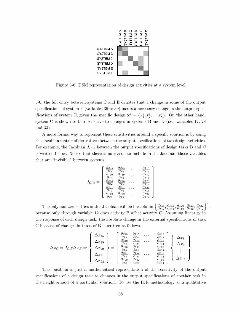
Figure 3-6: DSM representation of design activities at a system level
3-6, the full entry between systems C and E denotes that a change in some of the outputspecifications of system E (variables 36 to 39) incurs a necessary change in the output spec-ifications of system C, given the specific design x∗ = {x∗1, x∗2, . . . x∗κ}. On the other hand,system C is shown to be insensitive to changes in systems B and D (i.e., variables 12, 28and 33).
A more formal way to represent these sensitivities around a specific solution is by usingthe Jacobian matrix of derivatives between the output specifications of two design activities.For example, the Jacobian JB,C between the output specifications of design tasks B and Cis written below. Notice that there is no reason to include in the Jacobian those variablesthat are “invisible” between systems.
JC,B =
∂x15∂x8
∂x15∂x9
· ∂x15∂x14
∂x19∂x8
∂x19∂x9
· · · ∂x19∂x14
∂x20∂x8
∂x20∂x9
· · · ∂x20∂x14
∂x21∂x8
∂x21∂x9
· · · ∂x21∂x14
∂x22∂x8
∂x22∂x9
· · · ∂x22∂x14
The only non-zero entries in this Jacobian will be the column
{∂x15∂x12
, ∂x19∂x12
, ∂x20∂x12
, ∂x21∂x12
, ∂x22∂x12
}T,
because only through variable 12 does activity B affect activity C. Assuming linearity inthe response of each design task, the absolute change in the external specifications of taskC because of changes in those of B is written as follows.
∆xC = JC,B∆xB ⇒
∆x15
∆x19
∆x20
∆x21
∆x22
=
∂x15∂x8
∂x15∂x9
· · · ∂x15∂x14
∂x19∂x8
∂x19∂x9
· · · ∂x19∂x14
∂x20∂x8
∂x20∂x9
· · · ∂x20∂x14
∂x21∂x8
∂x21∂x9
· · · ∂x21∂x14
∂x22∂x8
∂x22∂x9
· · · ∂x22∂x14
∆x8
∆x9
...∆x14
The Jacobian is just a mathematical representation of the sensitivity of the output
specifications of a design task to changes in the output specifications of another task inthe neighborhood of a particular solution. To use the IDR methodology at a qualitative
68

level for complex systems, it is necessary to have an aggregate metric for this sensitivity.This metric can be some norm of the Jacobian, e.g., this metric can be the element-wiseEuclidean norm.2. Then the S-DSM representation of the system for that specific solutioncan be a square matrix whose entries i, j are that norm of the Jacobian calculated at thespecific solution x∗.
SDSMC,B =∥∥J∗
C,B
∥∥Nevertheless, even though it is useful to be able to express rigorously the entries of the
SDSM at the component and subsystem level, this level of detail is not useful in practice.When using an activity-based SDSM, the design team should be prepared to abstract andestimate qualitatively the effect of changes in output specifications on other activities. For-mulating the SDSM requires that the interaction in row i and column j be interpreted as”the change necessary to design activity i because of a unit change in activity j. In otherwords, if the design variables of component i are not (significantly) constraining those ofcomponent j in the neighborhood of the specific solution x∗, then the entry i, j should bezero. Using this convention, the S-DSM can be a relatively small matrix representing andsummarizing a design process of possibly thousands of design variables.
With this convention, all the concepts developed in the first part of this Chapter aretransferable to component-based DSM’s; the difference is limited to the way sensitivities arequantified. In the variable-based SDSM, sensitivity is objectively defined to be the relativechange in one variable as a consequence of a change in another. In the component-basedSDSM, sensitivity is subjectively defined as the change necessary in one component as aconsequence of change in another. In other words, since components are described by manyvariables, designers should simply use judgment as to whether the design of a componentinfluences the design of another.
3.4.2 Exogenous parameters and change propagation
As before, the SDSM of the design tasks can include functional requirements and charac-teristics. For example, for an automobile the functional characteristics or requirements canbe passenger volume, cargo volume, towing capacity, fuel economy or acceleration. Thesefunctional requirements usually represent the value of the product system to the user or thebuyer. Functional requirements are seldom mapped one-to-one to design variables. A sys-tem where such one-to-one mapping is possible is called an “uncoupled” design (Suh 1990).In most occasions, functional requirements will affect (and be determined as a function of)multiple design variables. In Figure 3-7 the functional requirements and aggregate designvariables appear on the same DSM.
2This is denoted ‖·‖. For any matrix A with elements Aij , its Euclidean norm is ‖A‖ =∑
i,j
√A2
ij
69

Figure 3-7: System-level DSM, extended to include functional requirements
The conditions that ensure that a design activity p can be common between variantsystems are similar to equations 3.12 and 3.13
∥∥J∗p,c
∥∥ = 0 ∀p, c∥∥∥J∗p,j
∥∥∥∆FRj = 0 ∀j
where the index c denotes a customized activity. In words, platform design activities mustbe insensitive to changes in functional requirements between the variants considered Also,platform variables must be insensitive to customized variables for the variants considered.For example, assume that FR1 is different between two or more variants. Applying the IDRalgorithm to the SDSM in Figure 3-7 yields the following partitioning into changes, invariantdesign rules (platform systems) and customized systems (Figure 3-8). The Invariant DesignRules in this case, i.e., the platform components, are only C and E; system A is not, eventhough it is not directly affected by the changing functional requirement 1. This is becauseit is sensitive to design changes in system B, which has to change because it is directlysensitive to changes in FR1.
3.5 Exploration of platform strategies
The SDSM representation and the IDR methodology can be used to facilitate the explorationof different platform designs and strategies. The application of the IDR algorithm can beused at the variable or at the system/component level to indicate the system elements thatdo not need to change between two systems of similar architecture that are required tosatisfy different functional requirements. Two extensions are presented in this section: (a)the effect of removing entries from the SDSM, and (b) the exploration of platform strategiesat multiple levels of system aggregation simultaneously.
70
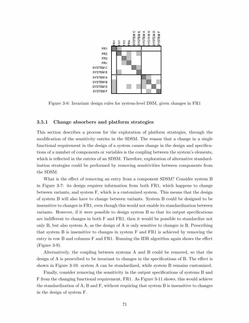
Figure 3-8: Invariant design rules for system-level DSM, given changes in FR1
3.5.1 Change absorbers and platform strategies
This section describes a process for the exploration of platform strategies, through themodification of the sensitivity entries in the SDSM. The reason that a change in a singlefunctional requirement in the design of a system causes change in the design and specifica-tions of a number of components or variables is the coupling between the system’s elements,which is reflected in the entries of an SDSM. Therefore, exploration of alternative standard-ization strategies could be performed by removing sensitivities between components fromthe SDSM.
What is the effect of removing an entry from a component SDSM? Consider system Bin Figure 3-7: its design requires information from both FR1, which happens to changebetween variants, and system F, which is a customized system. This means that the designof system B will also have to change between variants. System B could be designed to beinsensitive to changes in FR1, even though this would not enable its standardization betweenvariants. However, if it were possible to design system B so that its output specificationsare indifferent to changes in both F and FR1, then it would be possible to standardize notonly B, but also system A, as the design of A is only sensitive to changes in B. Prescribingthat system B is insensitive to changes in system F and FR1 is achieved by removing theentry in row B and columns F and FR1. Running the IDR algorithm again shows the effect(Figure 3-9).
Alternatively, the coupling between systems A and B could be removed, so that thedesign of A is prescribed to be invariant to changes in the specifications of B. The effect isshown in Figure 3-10: system A can be standardized, while system B remains customized.
Finally, consider removing the sensitivity in the output specifications of systems B andF from the changing functional requirement, FR1. As Figure 3-11 shows, this would achievethe standardization of A, B and F, without requiring that system B is insensitive to changesin the design of system F.
71

Figure 3-9: Effect of removing the sensitivity of B to FR1 and F
Figure 3-10: Effect of removing the sensitivity of A to B
This example shows that the removal of the sensitivity of system A to system B madeit possible to standardize A; the removal of the sensitivity of B to both F and FR1 enabledthe standardization of both A and B, but the removal of sensitivity of B to FR1 aloneachieved nothing; finally, the removal of sensitivity of B and F from FR1 achieved thestandardization of A, B and F as a cluster. This shows that there are many differentways to achieve standardization of specific components. To conclude which one is the beststrategy, it is useful to examine exactly what it means to remove an entry from an SDSM.
Removing an entry i, j from an SDSM prescribes that there should be no need forinformation flow from design activity j to design activity i, when the outputs of j are slightlychanged. This means that the design of i is required to be unconstrained by the outputsof activity j; i.e., that the design of j has some slack. Such a slack can mean that system i
needs to be over-designed, which in turn implies an economic penalty. For example, considerthe design of an electric motor and the battery in a power tool as two coupled systems. If
72

Figure 3-11: Effect of removing the sensitivity of systems F and B to FR1
the power requirement of the motor and the battery’s capacity are determined together,so that each one is a constraint for the other, then the corresponding SDSM should havesymmetrical entries in the corresponding rows and columns. Removing the entry in the rowof the battery and the column of the motor implies that the battery is designed first, andits design drives the design of the motor. Therefore, the power requirement for the motorwill be at most what the battery can provide; the battery will be generally oversized for thespecific motor. Consequently, small variations in the power requirement of the motor do notaffect the design of the battery. Effectively, such a design can accommodate different motorsas long as they do not constrain the design of the battery. Over-sizing is only one way totechnically remove SDSM sensitivities by intervening with the physical design. Anotherway is by training modules, e.g., using batteries in series. Yet another way, e.g., for physicaldimensions or information, is by provisioning for interface components between coupledsystems, so that the interface and at least one of the coupled systems are standardized,while the other is customized (Baldwin & Clark 2000). All these approaches to removingSDSM couplings imply that the design of a component is not constrained by the designof other components. In turn, this implies constraining the system away from its optimaldesign point, towards the interior of the feasible space and thus to suboptimal solutions.Therefore, the platform designer should remove as few sensitivities as possible.
On the other hand, removing entries enables the standardization of system componentsand the creation of platform strategies. In Figure 3-10, a single entry was removed, andthis resulted in the standardization of one system; in Figure 3-9, two entries were removedwhich resulted in 2 systems standardized. Generally, not all platform strategies carry thesame benefits, even if they involve the same number of standardized systems. The removalof entries should weigh the sub-optimality created by rendering two activities independent,against the benefits from designing more standardized components.
Figure 3-12 shows a plot of 100 standardization strategies, i.e., alternative combinations
73

of removed SDSM entries, applied to the system-level SDSM of Figure 3-8 ; the horizontalaxis stands for the number of entries removed in each trial, against the total number of stan-dardized elements (including functional requirements). Due to overlap, the points shown onthe plot are only 19. The plot demonstrates that there are different combinations of SDSMentries that can be removed and result in the same number of standardized components.Each of these alternative standardization strategies contains useful information, as it leadsthe engineering team to create buffers and standardization opportunities by intervening atdifferent places in a fully coupled and integral design.
Figure 3-12 shows just a simple 2-dimensional example of the search for platform strate-gies, where the number of SDSM entries removed must be minimized, and the number ofstandardized systems must be maximized. In this case, the points along the North-EastPareto frontier correspond to Pareto-optimal standardization strategies. The concept canbe extended to the general case where platform benefits do not depend directly on thenumber of standardized components, but are a function of the standardized componentsbetween two or more systems. These benefits may be the reduction in implementation cost,design time and construction cycle for the second development as well as the operationalefficiency in terms of maintenance and spare part inventory costs.
Figure 3-12: Removing SDSM entries: simulation results
3.6 Multi-level platforms
Fully standardizing or fully customizing an entire system may not always be the optimalstandardization strategy. This section shows how the IDR methodology can be used it-
74

eratively in hierarchical systems to allow platform strategies at various levels of systemaggregation. Consider system A in Figure 3-8, which is necessarily customized due to itsclose coupling with system B. If the design team has reasons to standardize system A, thenit might be worth exploring at least its partial standardization.
Observe that the coupling of systems A and B makes it possible to decompose systemA further into subsystems/components A1, A2 and A3, as shown in Figure 3-13 at thevariable level. This decomposition may be evident in the physical architecture of systemA, or it may require a change in the system’s architecture. The particular decompositionreveals the (1) the close coupling of component A3 with system B (which is not examinedat a lower aggregation level), (2) the feedback of information from the design of system Bto the design of system A2, and (3), the feed-forward of information from A1 to B. At thesubsystem level SDSM, this effect is shown in Figure 3-14.
Figure 3-13: Decomposition of system A at the variable level
Applying the IDR algorithm to the SDSM in Figure 3-14 shows that “exploding” systemA to subsystems enables its partial standardization (Figure 3-15). Indeed, subsystem A3 isnow part of the platform, whereas A1 and A2 are customized between variants.
At this time, there is no systematic way to explore which subsystems should be explodedinto their components. There are two approaches: as described above, a customized systemwhose potential benefit from standardization is large may be exploded to its componentsin case some can become part of the platform. The potential can be explored with thesimulation methodology explained in the previous section. Similarly, a standardized system
75

Figure 3-14: Decomposition of system A at the subsystem level
Figure 3-15: Re-partitioned SDSM, with platform that includes subsystem-level line items
may be investigated for components that can be customized, if this should greatly improvethe performance of the system. However, these approaches require a fully quantified systemand benefits model.
3.7 Summary
This chapter presented a novel methodology for the identification of the variables and com-ponents that do not need to change (i.e., platform variables and components), given aparticular design and different functional requirements for variants in a product family.Next, this section introduced two methodologies for the exploration of alternative stan-dardization opportunities and platform designs. One is based on simulation and requires anapproximation model for the potential benefits and penalties of standardization strategies;the other is based on engineering judgment and enables the exploration of standardization
76

opportunities on various levels of system aggregation.
77

78

Chapter 4
Flexibility valuation in large-scale
engineering programs
4.1 Introduction
A program’s flexibility is captured in the developer’s ability to defer design and developmentdecisions until uncertainty unfolds and more information becomes available. Flexibility isalso related with the developer’s range of future choices. In a program of platform-basedprojects, the developer’s flexibility was modeled as the choice of alternative standardizationchoices for the second and subsequent developments in the program. Chapter 3 introduceda methodology for screening alternative standardization strategies. Chapter 2 cited exam-ples from the literature that demonstrate that this flexibility has value and should guidedevelopment decisions for the early stages of the program. This chapter shows how thisvalue can be estimated.
The concept used for the valuation of flexibility is real options. The methodology orig-inates from the financial economics literature in the 1970’s, and there have been recent,mostly academic attempts to “import” it to the engineering valuation practice. These at-tempts have focused on case studies that demonstrate the concept and use of real optionsin the valuation and optimization of engineering systems. Applications include phased de-ployment of communication satellite constellations under demand uncertainty (de Wecket al. 2003); decisions on component commonality between two aircraft of the same family(Markish & Willcox 2003); building design under rent and space utilization uncertainty;e.g., see Zhao & Tseng (2003), Kalligeros & de Weck (2004), Greden & Glicksman (2004)and de Neufville et al. (2006). Despite these efforts however, the concepts and analyticaltools have had very little traction with practitioners.
It is postulated that the slow penetration of the real options methodology can be at-tributed to two main reasons. Firstly, most of the engineering literature on flexibility andreal options does not seem to agree on basic definitions and a single modeling approach.Often, flexibility is conceptualized as a collection of real options, (i.e., a right, but not an
79
obligation to change, expand, shrink or otherwise evolve a system) and this has had signifi-cant conceptual appeal to engineers. Indeed, the contribution of some of these case studiesis in conceptualizing the real options associated with the engineering problem, withoutattempting to provide a rigorous option analysis. On the other hand, none of these appli-cations provides a general, intuitive and consistent framework (or “language”) for modelingand communicating flexibility in engineering design.
The second reason for the slow penetration of real options in engineering practice isunderstood to be the attempt to transfer a “pure” and positive economic theory to the“production floor” of engineering design. When a rigorous options valuation is attemptedin engineering applications, it usually runs into theoretical errors, practical difficulties inapplication, and logical arguments that convince neither engineering nor finance-orientedaudiences. Adopting the theory requires a deep understanding of the assumptions behindit, which in turn, requires a level of economic literacy found in very few engineers. Evenwhen the assumptions and techniques are understood, they often do not apply convincinglyto the engineering problem at hand. And even when the assumptions are reasonable andthe analysis is correct, the practical application requires conceptual leaps of faith (e.g.,using the risk-free rate for discounting) and changes in well-established valuation practiceswithin an organization. Experience has shown that improving the financial sophisticationof engineering organizations has been slow and difficult.
In the context of this work, a useable methodology for flexibility valuation in an engi-neering management context is crucial. If the engineer is unable to estimate the flexibilityvalue created by standardization (or any other technical innovation, for that matter), thenthey have no visible and quantifiable guidance to design for it. With this rationale, a novelreal option valuation process is developed, that overcomes these impediments to the theory’slimited appeal in engineering. The proposed methodology deviates very little from current“sensitivity analysis,” practices in design evaluation. Firstly, a graphical language is intro-duced to communicate and map engineering decisions to real option structures and equa-tions. These equations are then solved using a generalized, simulation-based methodologythat uses real-world probability dynamics and invokes equilibrium, rather than no-arbitragearguments for options pricing.
For the solution of these equations and the valuation of alternative design decisions, anovel simulation-based methodology is presented in Section 4.3. The algorithm is basedon simulation and the stratified state aggregation techniques developed in the 1990’s byTilley (1993), Barraquand & Martineau (1995), Rayman & Zwecher (1997), Broadie &Detemple (1997), Broadie & Glasserman (1997) and others. It involves a step processof simulating the exogenous uncertainties (in their real probability measure), valuing one“reference” design alternative per the organization’s practices, and finally, valuing the otherdesign alternatives and options relative to the reference design, based on the organization’sinferred risk aversion and the system’s exposure to underlying risk. Certainty-equivalencearguments are used; risk-neutral dynamics are avoided. The implication of this approach is
80

that in some cases the proposed valuation methodology sacrifices economic rigor and someaccuracy, specifically, the methodology is incorrect (from an economic viewpoint) in thevaluation of partially correlated design alternatives or options on the maximum of severalunderlying assets. This sacrifice can be acceptable in the context of design and developmentif the valuation leads to an optimal design decision without necessarily a correct valuation.After all, the engineer’s motivation to use the real options method is not to do valuationfrom the viewpoint of a diversified investor; it is to optimize and select among alternativedesigns.1
Parking garage example As an example of the problems dealt with in thischapter, consider the design of a parking garage; see de Neufville et al. (2006).For simplicity, focus on the number of levels as the main design decision for theparking garage. Current engineering practice often involves building a garagewith the optimal number of levels based on an expectation of the demand forparking. An alternative approach is to build a garage with fewer levels, butwith reinforced columns that can support additional levels in the future. Thevalue of the smaller building includes the value of flexibility (a) to choose howmany levels to add to the existing garage in the future, and (b) to choose thetiming of this expansion. Because the optimal expansion of the garage is con-tingent on unknown future events (e.g., the parking demand realized), any priorcommitment to expand in the future is suboptimal. However, if the garage isdesigned based on a discounted-cash-flow value calculation, such commitmentis automatically assumed. The design of the smaller garage, i.e., the decisionon how many levels to build immediately and how many to be able to supportin the future, should be based on the value of flexibility to expand the garagein the future. The methods presented in this chapter can be used to frame andsolve problems such as the valuation of a garage design solution, considering theexpansion flexibility that it enables. The optimization of the design is not dis-cussed in this chapter. Because of its technical simplicity, this garage examplewill be used repeatedly in the text to clarify the concepts.
4.2 Design and development decisions
The managerial flexibility enabled by a particular design solution can be regarded for mod-eling purposes as strategic or operational (see Figure 2-6, p. 46). Strategic flexibility isusually taken to imply irreversible decisions, while operational flexibility often implies re-versible actions with a non-trivial switching cost. This section demonstrates how common
1Testing this “sacrifice” rigorously is outside the scope of this thesis. However, the design study in
Chapter 5 compares the results from a risk-neutral valuation to the ones obtained with this methodology,
and concludes that for the purposes of selecting design alternatives, the two approaches give the same results.
81

design and development decisions can be represented graphically as the exercise of strategicoptions and irreversible decisions. It is assumed that a single agent, the developer, has de-cision power over all current and future design or development decisions. It is also assumedthat at that level, the developer’s goal is to maximize present value or minimize the presentvalue of cost of operations.
The general idea is to model alternative designs or phases of an engineering programas income-generating “states,” and the transitions between states as the exercise of op-tions. These transitions occur in two main stages: design and construction. Constructionis modeled as the exercise of a call option on the difference in value between the targetand departure states, with an exercise price equal to the construction cost. This is calleda timing option, because it involves only the decision of when to begin construction andtransition to another state. Design involves choosing between alternative target states, andit is modeled as the exercise of an option on the maximum of several underlying assets (achoice option). Each of the underlying assets to a choice option is a timing option leadingto a target state. The total value of a state will be the sum of the value of its expectedcash flows, plus the value of all the choice and timing options it enables. The next sectionselaborate on these definitions of states, design and construction options.
4.2.1 Assets and states
A state represents the ownership and operation of a collection of assets, corresponding to aphase of program development. States describe a steady-state, business-as-usual situation,where minor, temporary and reversible interventions to a system’s operation are used tomaximize it’s performance; see Vollert (2003, p.23). The defining characteristic of thestates in a model is that the transitions between them are irreversible, so their definition isa modeling decision. For example, the ownership and operation of 3, 4 and 5 oil productionfacilities in a certain region can be defined as three different states. It is assumed that thesestates are managed optimally, generating revenues that give them their intrinsic value.Graphically, states can be represented with a simple rectangle and a short description ofthe assets in operation.
A state can be modeled as a function that returns the free cash flow generated, giventhe design characteristics of the assets in that state and all the relevant information knownto the organization at each time. For example, the monthly cash flows generated by aparking garage is a function of its capacity, the average monthly demand for parking there(in car-hours), the parking fees changed and the operating costs of the building. For morecomplex systems, the cash flows will depend on design variables and external informationin much more complicated ways. However, assuming that cash flows per time period can bedeterministic functions of the known design variables and uncertain factors, it is possibleto write cash flows as CFu(st), where u refers to a state and st is a vector containing allrelevant information at time t for determining the cash flow.
82

The value V cfu (s0) as of t0 of these expected cash flows can be written as the sum of
the discounted future expectation of the revenues. Equation 4.1 represents the traditionaldiscounted-cash-flow analysis (DCF) from time t0 to an ad-hoc terminal time T , wherebythe future cash flows from t = t0 . . . T are calculated based on the expected values of theuncertain parameters E[st] and then discounted back to the present time t0 at a discountrate r, which depends on the risks in these expected cash flows.
V cfu (s0) =
T∑t=t0
e−rtCFu(E[st]) (4.1)
A more correct approach is to calculate the expected future cash flows in differentscenarios of the uncertain parameters, and discount these expectations to the present time.Since the risk in the cash flows now depends explicitly on the design characteristics of stateu, the discount rate is written as ru to reflect this. The calculation, shown below, is knownas the “expected present value (EPV).”
E[V cf
u (s0)]
=T∑
t=t0
e−rutE[CFu(st)] (4.2)
The two calculations will give different results if the function CFu(st) is nonlinear in st
because of Jensen’s inequality (also known as the “flaw of averages”). This often happenswhen the state u incorporates (reversible) flexibility, in which case the function CFu(st) isnon-linear (Dixit & Pindyk 1994). For example, suppose that the vector st is the cost of gasand oil used in a factory for heat generation (Kulatilaka 1993). If a factory has no flexibilityto switch to the cheapest fuel at any time, then the value of the cash flows generated willbe linear in st. If a factory has such flexibility (e.g., because it owns a dual-fuel burneror two single-fuel burners with combined capacity larger than the peak demand), then thecash flows will be non-linear in st. This is because e.g., when gas is adequately cheaperthan oil, it will be optimal to produce energy using gas; the cost of energy will be a concavefunction of the cost of gas and therefore, free cash flows will be convex with the cost of gas.This non-linearity would cause the values calculated with the two methods not to agree.All but the simplest systems have such operational flexibilities, which means that Equation4.2 should be used for their valuation. In practice, the value of assets is often calculatedby considering the conventional DCF analysis (Equation 4.1) because it is a little simplercomputationally, even though it is flawed in principle.
The factor e−rut represents an appropriate factor for discounting future cash flows gen-erated from the operation of state u. In theory, this rate should match the risk in the cashflows in the nominator. In practice, these risks are considered ad-hoc to match the risk inthe value of the entire holding firm, and the discount rate is chosen to be the firm’s weightedaverage cost of capital (WACC).
Finally, in practice, the value of these expected cash flows is considered to be the totalvalue of the assets in a state. In reality, the value of these assets includes the value of
83

the real options to select and transition to other states by the design and development ofadditional assets. The next sections present the graphical convention and model for thesedecisions.
4.2.2 Decisions on timing
The ownership and operation of assets in a state may enable the transition to other states,through the expansion or exchange or re-configuration of existing assets or the acquisitionof new ones. The option to transition from state u with value of expected cash flows V cf
u
to state w with value of expected cash flows V cfw at a transition cost Cuw is a call option on
V cfw −V cf
u with a strike price Cuw. If we assume that the decision-maker makes the optimalchoice between the transition and waiting for any value of the uncertain parameters st, thevalue of this option at time t is the maximum of its immediate exercise or its expected valuein the future.
Fuw(st) = max[[Vw(st)− Vu(st)]− Cuw, e−ruwδtE[Fuw(st+δt)
](4.3)
where δt is the time increment used for calculations and ruw is an appropriate discount ratefor the option’s future expected value (continuously compounded). Timing options can berepresented graphically as shown in Figure 4-1. If the option is not available over a periodof time, but only instantaneously on a specific date, then it can be shown with a diamondinstead of an arrow (Figure 4-2).
The total value of state u will include the intrinsic value of the income generated by theassets in that state, plus the value of the option value to transition to state w, so that
Vu = V cfu + Fuw
Parking garage example The owner of a 4-level parking garage whose columnscan support up to 5 levels has the real option to expand the garage by buildinganother level. Barring any specific constraints, this decision can be made atany time. The total value of the 4-level garage is the value of its future cashflows plus the value of the option to exchange the expected value of 4-levelsand construction cost, to obtain the value of a 5-level garage. When developersdecide to expand the building, the value of the transition option will be equalto the value of a 5-level garage less the construction cost of an additional level.
With this formulation, the exercise of a timing option implies an irreversible transitionbetween states. To see this, suppose that at time t∗ it is optimal to exercise the timingoption and obtain state w. Then the total value of state u at t∗ will be the value of statew net of construction costs:
Vu(st∗) = V cfu (st∗) + Fuw(st∗)
= V cfu (st∗) + Vw(st∗)− V cf
u (st∗)− Cuw
= Vw(st∗)− Cuw
84

If the option expires at T , its value then is
Fuw(sT ) = max [[Vw(sT )− Vu(sT )]− Cuw, 0]
Option expiration can happen in cases of concession periods for the development of landor natural resources (Brennan & Schwartz 1985). Often, option expiration is considerednaturally, when the assets in states u or w die. However, in many cases, both statesand these options are perpetual and the time horizon is used only to enable spreadsheetcalculations.
Figure 4-1: An American timing option to obtain state w from state u: transition can occurat any time within a time horizon.
Figure 4-2: A European option to obtain state w from state u: transition can occur onlyat a specific time.
Time-to-build
Suppose the transition between states u and w is not instantaneous, but requires time-to-build ttb, after which the entire construction cost Cuw is paid in full (Majd & Pindyck 1987).Equation 4.3 above can be modified so that the value of immediate exercise of the option,I(st), reflects this:
Fuw(st) = max[I(st), e−ruwttbE[Fuw(st+ttb)
]where
I(st) = e−rwttbE [Vw(st+ttb)]− e−ruttbE [Vu(st+ttb)]− e−rf ttbCuw
(4.5)
This assumes that the developer commits at time t to receive the value of state w at timet + ttb, Vw(st+ttb), in exchange for the value of the cash flows in state u and the presentvalue of the construction cost. Since the expected values of the states are uncertain, theyare discounted at an appropriate rate. If the construction cost is considered certain andsince the developer has committed to paying it, it can be discounted at the risk-free raterf .
85

The effect of a high ttb is to reduce the value of the option, because of the differencein incomes foregone during the time to build. Such a time to build can be representedgraphically as shown in Figure 4-3.
Figure 4-3: An American option with time-to-build ttb
4.2.3 Decisions on target state
To model design decisions, the proposed approach uses choice options, i.e., options on themaximum of several underlying assets. The payoff of an option to obtain the maximum ofV1(st) . . . Vh(st) at a respective cost D1(t) . . . Dh(t) is max
i=1...h(Vi(st)−Di(t)). Therefore, if
the option does not need to be exercised immediately, its value at time t is the maximumof the payoff and the value of waiting. The value of waiting is the expected value of theoption in the future, discounted at an appropriate rate rOR:
OR(st) = max[
maxi=1...h
(Vi(st)−Di(t)) , e−rORδtE[OR(st+δt)]]
(4.6)
Choice options can be used to model design decisions, because design involves choosingbetween alternative engineering solutions, and locking-in with these solutions (e.g., by ob-taining permits, securing contracts or other licences). In this work, the following conventionsare used:
• The exercise of a choice option is irreversible.
• Whether alive or exercised, choice options do not affect the income generated byexisting assets (therefore the intrinsic value of the current state).
The first convention may seem restrictive, but in practice it often is not. Design choicescan often be considered irreversible, because the cost and time required are so large thatrepetition of the process is prohibitive. Nevertheless, if a design decision needs to be con-sidered reversible, this is possible by stacking sequential choice options (see Section 4.2.4).Finally, Equation 4.6 can be easily extended to consider time lags in design as well.
Parking garage example The owner of a 3-level garage is modeled to have achoice option between expanding to either 4 or 5 levels. The owner may postponethe decision, which cannot be taken back once made. Deciding between 1 or 2additional levels incurs design costs, but does not imply that these additionallevels will be built; the developer obtains the timing option to build 1 or 2
86

additional levels, whichever was decided at the choice option. In other words,the exercise of a choice option does not imply a change in state. Graphically,this situation can be represented with the OR node as shown in Figure 4-4. Thefigure also shows how the owner of a 4-level garage does not have the choiceoption that the 3-level garage entails. Based on the above, the value of the 3-level garage V3(st) is the sum of the value of future cash flows V cf
3 (st), plus thevalue of the choice option between expanding by one or two additional levels.Exercising the choice option obtains the timing options to construct the chosendesign, F34(st) and F35(st).
V3(st) = V cf3 (st) + OR(st)
= V cf3 (st) + max
[(F34(st)−D34) , (F35(st)−D35) , e−rORδtE[OR(st+δt)
](4.7)
Suppose that at time t∗, it was optimal to design one more additional level; thetotal value of the 3-level garage would become
V3 = V cf3 (st∗) + OR(st∗)
= V cf3 (st∗) + (F34(st∗)−D34)
(4.8)
i.e., the intrinsic value of its future cash flows plus the (net) value of the optionto build one more level. If t∗ was also the optimal time to exercise the timingoption, then the total value of a 3-level garage would become
V3 = V cf3 (st∗) + (F34(st∗)−D34)
= V cf3 (st∗) + V4(st∗)− V cf
3 (st∗)− C34 −D34
= V4(st∗)− C34 −D34
i.e., the value of a 4-level garage net of design and construction costs.
Figure 4-4: Choice between development options to 4- and 5-level garage
4.2.4 Complex design and development structures
With the convention introduced, choice and timing option can be combined to model a lim-itless variety of design and development decisions. The parking garage example is extendedto illustrate how.
87

Parking garage example The structure of design and development decisionsin Figure 4-5 encompasses much of the flexibility available in a typical project,in the context of the familiar parking garage. According to the model in Figure4-4, the owner of a 3-level garage had the choice between designing a 4- or a 5-level garage. Suppose now there are more design choices, e.g., as to the materialof the additional levels. The owner of 3 levels has the initial design decision ofhow many levels to add; if the choice is “2 more” then there is choice as to theirmaterial: they can both be concrete or both be steel. Each choice associated witha different construction time lag (TtBcc and TtBss). If the optimal initial choiceis “1 additional level,” then the second choice option (OR2) gives the developera chance to change the decision to “2 additional levels.” If the developer decidesin node OR2 to expand to a 4-level garage, they have the choice of material onceagain. A 4th floor out of concrete allows the subsequent choice (OR3) of thematerial of the 5th level (when it is built). A 4th floor of steel requires that the5th level is also out of steel, but subjects the developer to, say, a possible changein legislation that will restrict the construction of more than one steel levels atopa concrete structure. This last uncertainty is shown using a circular “chance”node which assigns probabilities to its branches, much like in a decision tree. InFigure 4-5, the chance node serves to reduce the the value of the option to builda second steel floor is reduced by the probability the the legislation passes.
Figure 4-5: A complex structure of development decisions
4.3 Valuation
In the outset, it was postulated that the premise of existing valuation theory, i.e., the abilityto hedge on the underlying asset and the lack of arbitrage, is part of the reason that thereal options method has not gained traction with designers and developers. No-arbitrage
88

arguments enable the precise calculation of real options as pure derivative assets, when theunderlying asset is actively traded, liquid and its value is observable. In all other cases,invoking no-arbitrage and using risk-neutral probabilities can be far-fetched, besides makingthe entire methodology unconvincing. This is the motivation for (yet) another solutionmethodology. The valuation methodology proposed in this chapter is designed to appeal toengineers by being conceptually close to current valuation and “sensitivity analysis” testingof design and development programs. To achieve this, we suggest compromising some ofthe theoretical rigor of “pure” real options analysis.
In the proposed methodology, a single reference state is valued using the developingorganization’s standard practices. The reference state corresponds to the base case design,i.e., the solution the developer would consider before any discussion about flexibility. Thisvaluation implicitly provides the organization’s risk tolerance towards the uncertainties st
governing the system’s value. This risk tolerance is used for the valuation of alternativesystem designs (states) and options to reconfigure the system in the future (transitionsbetween states). The valuation of options and states is achieved using an original simulationmethod which builds on the stratified state aggregation method along the payoff (SSAP)(Barraquand & Martineau 1995) and the Generalized Multi-Period Option Pricing model(Arnold & Crack 2003).
Figure 4-6 shows graphically the characterization of the proposed valuation scheme alongfour dimensions: state-space modeling, value dynamics modeling, decision rules and valua-tion. Monte-Carlo simulation is used to model the state space, as it is far more appealingto the engineering community than both lattices and continuous-time formulations. Forthe same reason, the proposed method involves simulating the external uncertainties tothe engineering system and deduce the value of the system for a representative value ofgroups of simulation events; alternative approaches involve identifying a portfolio of secu-rities that is believed to perfectly track the value of the system, or explicitly assuming thevalue of the system follows a Geometric Brownian Motion; e.g., see Copeland & Antikarov(2001). Both these alternatives may be reasonable and easily acceptable in financial assetvaluation, but are often not convincing to the engineering community or imply absurd as-sumptions for many technical systems. The proposed method involves recursive calculationof the decision rules using stratified state aggregation (Barraquand & Martineau 1995).Alternative simulation approaches include the arbitrary specification of decision rules ortheir parametrization; e.g., see Longstaff & Schwartz (2001) or Andersen (2000). Finally,valuation is performed by discounting future values across alternative designs and optionsso that the price of risk is retained constant. This is achieved using the Generalized Multi-Period Option Pricing model (Arnold & Crack 2003), which avoids the need to simulaterisk-neutral paths.
The methodology introduced in this chapter uses the state aggregation technique pro-posed by Rayman & Zwecher (1997), and applies it explicitly on the space of uncertainfactors s. In other words, for N uncertain factors and M number of bins for each factor,
89

Figure 4-6: Characterization of the proposed option valuation methodology (shaded boxes)and comparison with other valuation approaches.
the methodology proposes a grid of MN , N -dimensional bins. These bins are defined foreach time step with a small first-stage simulation of the uncertainty space. Rayman &Zwecher (1997) suggest 25 sample paths for each bin in this first stage simulation are ade-quate, and find that increasing the number of paths has a negligible effect on the results.For each time t, the bins are defined as hyper-cubes; e.g., for 2 uncertainties, Figure 4-7shows a bin definition where the bin sizes increase exponentially.
The next step is to simulate a full set of K paths using their real-world (not risk-neutral)distributions for the uncertain factors, as described in Section 2.6.2. Rayman & Zwecher(1997) recommend K = 500 per bin. Next, for each time t = t0 + δt...T and for each binm = 1...M it is possible to calculate
1. the average value for each uncertain factor in each bin smt , as
smt =
1at(m)
∑all pathsin bin mat time t
smt
where smt denotes a path in bin m at time t, and at(m) is the total number of paths
in bin m at time t. As the number of paths in bin m at time t increases, the averagevalue sm
t will converge to a representative value for that bin. The rest of the analysisuses only these values sm
t to represent a bin (and not e.g., its bounds or paths in it,see Figure 4-7). For t = t0, the bin specification is trivial: the factors are known withcertainty and there is only one bin containing all paths, so sm
t = sm0 = s0.
90

2. the transition probabilities between all the bins at time t with all the bins at timet + δt. Denoting bt(m, n) the number of paths than fall in bin m at time t and binn at time t + δt, the transition probability from bin m to n can be estimated as the(m,n)-element of a matrix Pt:
Pt(m,n) = bt(m,n)/at(m)
Figure 4-7: Two-dimensional bin definition and some representative values at time t
For calculating at(m), bt(m,n) and smt , the paths do not need to be kept in memory.
Since they are additive statistics, at(m), bt(m,n) and smt can be updated as each simulated
path is considered. After all paths have been accounted for, the final values of at(m),bt(m, n) and sm
t are used to represent bins and to calculate the transition probabilitiesPt(m,n).
4.3.1 Calculation of conditional expectations
With these background calculations it is possible to estimate the conditional expectationson the space of uncertainties. For example, denoting E[st+δt; sm
t ] the expected value of theuncertain factors st+δt conditional on the event that the value of the uncertain factors at t
falls in bin m,
E[st+δt; smt ] =
∑n
Pt(m,n)snt+δt (4.9)
Equation 4.9 can be used to estimate conditional expectations of future values or cashflows, such as the ones found in Equations 4.2, 4.3 and 4.6. For example, with this stateaggregation scheme, the expected cash flows as of t = t0 in Equation 4.2 can be estimatedas
E[CFu(st+δt); smt ] =
∑n
Pt(m, n)CFu(snt+δt)
From now on, Em
[st+δt] is taken to mean E[st+δt; smt ] for brevity.
91

The calculation of the conditional expectation for more than one time steps into thefuture can be constructed directly from the definition of the transitional probabilities andBayes’ rule. Consider the conditional probability between sm
t and snt+2δt. The probabilities
of reaching bin n from each bin at the previous time step (time t + δt) are contained in then’th column of Pt+δt. The probability of reaching the bins at t + δt from bin m at time t
corresponds to the m’th row of Pt. Therefore, the probability of reaching snt+2δt from sm
t
is the (m, n) entry in Pt+δtPt. Generally, the transition probability between smt and sn
t+jδt
where j is an integer is the (m,n)-element of the matrix PtPt+δt . . . Pt+(j−1)δt.
4.3.2 Valuation of a reference design
In contrast with the existing simulation algorithms described above, the proposed methodinvolves simulation of the real-world dynamics of the underlying uncertainties st, valuationof a reference design based on its expected future cash flows (Equation 4.2) excluding anyflexibility, and estimation of the developer’s implied price of risk for the uncertainty to whichthe reference design is exposed to. Consider a reference design, its corresponding state andan ad-hoc acceptable discount rate rref for this design. The value of this state Vref as oftime t0 without any choice or timing options associated with it is given in Equation 4.2.Re-writing this for the representative values in bins, instead of the simulated paths, givesEquation 4.10.
Vref (s0) =T∑
t=t0
e−rref tE[CFref (st)] (4.10)
where the expectation is taken over all bins n at each time t. Alternatively, this value canbe calculated recursively starting from t = T and going backwards (equation 4.11). Therecursive calculation is preferred over the previous one, because it yields the value of thereference design Vref (sm
t ) for all t = t0 + δt...T and for all bins m = 1...M .
Vref (smt ) = e−rref δt E
m[Vref (st+δt)] (4.11)
Because of the uncertainty in future values, the discount rate for the reference case willalso be equal to the risk-free rate at which the developer can lend money (e.g., by buyinggovernment bonds), plus a risk premium, which is assumed for simplicity to depend onlyon the reference design, so that
RPref = erref δt − erf δt
The fact that the organization requires a risk premium for the uncertainty in the underlyingfactors means that there is an implicit “price of risk” for these uncertainties within theorganization. If risk is measured in standard deviation of expected future returns, then theprice of risk λ can be defined as the “required risk premium per unit of standard deviationof expected returns.” For the valuation of the reference design, it can be calculated as
92

shown in Figure 4-8 and equation 4.12.
λ =erref δt − erf δt
σref(4.12)
Figure 4-8: Inferred price of risk from reference design valuation
Although the price of risk is almost never explicitly discussed for the valuation of adesign, most organizations are comfortable establishing a discount rate rref to compensatefor the risks in the future expected values of Vref (s0). rref will often be the weighted-averagecost of capital (WACC) of the firm, implying the assumption that the project correspondingto state u is representative of the entire firm in terms of risk exposure to the uncertaintiess. Although in theory this should make no difference in the valuation, we recommend theuse of the first state in the development of a program as the reference state (e.g., state u inFigure 4-5). The reason is that the first state will probably represent a design the developeris more comfortable valuing, perhaps because of better technical knowledge.
4.3.3 Valuation of two perfectly correlated states
To value another state w, whose value is perfectly correlated with the reference design, thedeveloper has two obvious choices for the discount rate: (a) they may use the referencediscount rate rref , or (b) use the same price of risk. In practice, the firm-wide WACC isalmost always used to value all designs. However, unless the reference state and state w
have no differences in risk exposure to st, using the WACC for both implies an inconsistency,i.e., that the developer is indifferent to the uncertainty in future values (see Figure 4-9).Suppose the standard deviation of changes in future values of design w are smaller than forthe reference design. Using the reference discount rate for future values of w implies thatthe developer places no value in the difference in risk, σref − σw, which is inconsistent withthe fact that a risk premium RPref is demanded for the risk σref , given that the referencedesign and w are perfectly correlated. In other words, if design w is traded in the market ata fixed price, set by other developers with the same risk tolerance (therefore the same λ),
93

then the developer will wrongfully not want to invest in w. Conversely, if w was riskier thanthe reference state, the developer using rref to value both will think w is a good design,when in fact it will not be. In conclusion, design w cannot be consistently valued using thereference discount rate rref .
Figure 4-9: Risk and discount rate for design w
Therefore, w has to be valued at a discount rate rw 6= rref , so that the price of risk invaluing both states is constant (for a discussion on this argument, see Section 4.4). Theproposed methodology holds the price of risk λ constant, and uses certainty-equivalentvaluation for all designs other than the reference one. The value of design w can be writtenas a certainty-equivalent as follows.
Vw(st) = e−rwδtE[Vw (st+δt)]⇒ (erwδt + erf δt − erf δt)Vw(st) = E[Vw (st+δt)]⇒ (erwδt − erf δt)Vw(st) + erf δtVw(st) = E[Vw (st+δt)]
which means
Vw(st) = e−rf δt[E[Vw (st+δt)]− (erwδt − erf δt)Vw(st)
]= e−rf δtCEQ
[Vw (st+δt)
] (4.13)
Equation 4.13 shows that the same present value can be obtained either by discountingthe real expected value at a rate that reflects the risk inherent in the expectation, or byreducing the future expected value by a certain amount that depends on its risk, and thandiscounting it at the risk-free rate. The value CEQ [Vw (st+δt)] is referred to as the certaintyequivalent value and is equal to the expected future value E[Vw (st+δt)] minus a certainamount that corresponds to the risk in the expected value of design w. This amount isthe required risk premium (which is unknown) times the actual value of w at time t, which
94

is also unknown. However, their product (erwδt − erf δt)Vw(st) can be estimated as shownbelow. Holding the price of risk constant between the valuation of the reference design andw means
λ =erref δt − erf δt
σref=
erwδt − erf δt
σw
It follows thaterref δt−e
rf δt
σref= erwδt−e
rf δt
σw
⇒ erref δt−e
rf δt
Std
[Vref (st+δt)
Vref (st)
] = erwδt−erf δt
Std
[Vw(s
t+δt)
Vw(st)
]⇒ (e
rref δt−erf δt
)Vref (st)Std[Vref (st+δt)]
= (erwδt−erf δt
)Vw (st)Std[Vw (st+δt)]
or,
(erwδt − erf δt)Vw (st) =Std[Vw (st+δt)]Std[Vref (st+δt)]
Vref (st)(erref δt − erf δt) (4.14)
Substituting Equation 4.14 into 4.13 yields the value of w given the risk tolerance ob-tained from valuing the reference design:
Vw (st) = e−rf δt
[E[Vw (st+δt)]− (erref δt − erf δt)Vref (sm
t )Std[Vw (st+δt)]Std[Vref (st+δt)]
](4.15)
Equation 4.15 can be used directly with the state aggregation scheme described in theprevious section for the recursive valuation of design w. For each bin m at time t, theexpected value of w in the next time step over all the bins n in time step t + δt is shown inEquation 4.16. The standard deviation of Vw (st+δt) given Vw (sm
t ) is denoted Stdm
[Vw (st+δt)]and is calculated easily in Equation 4.17.
Em
[Vw (st+δt)] =∑
n
Pt(m,n)Vw (snt+δt) (4.16)
Stdm
[Vw (st+δt)] =√
Em
[Vw (st+δt)2]− Em
[Vw (st+δt)]2
=
√∑n
Pt(m,n)Vw (snt+δt)
2 −(∑
nPt(m,n)Vw (sn
t+δt))2 (4.17)
4.3.4 Valuation of timing options
The value of a timing option to obtain state w in exchange for the value of u and thedevelopment cost is perfectly correlated with the difference Vw (st)− Vu(st), if u and w areperfectly correlated. Therefore, if the two states u and w are perfectly correlated betweenthem then the analysis in the previous section applies and the value of holding the optionalive can be estimated recursively using Equations 4.15, 4.16 and 4.17. Ideally, the referencedesign should be the option’s underlying asset, i.e., Vw (st)−Vu(st); however, the appropriatediscount rate for valuing this difference will not be known normally. On the other hand, ifthe two states are perfectly correlated, either one can be used as a reference case. Moreover,if they are both perfectly correlated with another reference state Vref , then that value can
95

be used as a reference. So generally, the value of holding the option in bin m at time t isestimated as
H (smt ) = e−rf δt
[Em
[Fuw (st+δt)]− (erref δt − erf δt)Vref (smt )
Stdm
[Fuw (st+δt)]
Stdm
[Vref (st+δt)]
](4.18)
The value of the timing option for each bin m at time t will be Fuw (smt ) = max[H (sm
t ), I (smt )],
where I (smt ) is the value of immediate exercise, I (sm
t ) = [Vw (smt )− Vu(sm
t )]−Cuw, assumingthat the time to build is zero. Extension to longer construction times is straight-forward,given Equation 4.5 and the calculation of multi-period conditional probabilities in Sec-tion 4.3.1. The optimal exercise region of the timing option is defined by regions in the(s1, s2, ..., sN , t) space in which it is optimal to exercise the option. It can be approximatedby the discrete set of points sm
t , m = 1...M, t = 0...T for which I (smt ) > H (sm
t ).
4.3.5 Valuation of choice options
Choice options are generally options on the maximum of several underlying assets. In thecontext of the decision model developed here, these alternative assets are the timing optionsto exchange state u for one of a set of h alternative states. These timing options are de-noted Fu1, ..., Fuh, with respective strike prices (construction cost) Cu1, ..., Cuh. The choiceoption to obtain each of these timing options will generally have a strike price Du1, ..., Duh,representing the cost to design each of the h assets. Assuming negligible design time lag,the general expression for the choice option is the maximum of immediate exercise, I (sm
t )and holding the choice option alive, H (sm
t ). The value of immediate exercise is
I = max [(F1(st)−Du1) , ..., (Fuh(st)−Duh)]
and the value of holding the option alive is given by Equation 4.18 above. As before, thevalue of holding the choice option is estimated in every bin m at time t by calculating itsexpected value at t + δt over all bins at that time, subtracting the dollar risk premium,and discounting at the risk-free rate (equations 4.15, 4.16 and 4.17). If all underlyingoptions Fu1, ..., Fuh are perfectly correlated, then any one of them can be used as a referencevaluation. Moreover, if they are in turn correlated with Vref , then Vref can be used directly.
4.4 Methodology performance and discussion
The previous sections addressed the modest penetration of the real options method in en-gineering design and development decisions. It was postulated that two impediments havebeen a common communication language for real options and a valuation methodology thatis approachable by engineering and technology practitioners. Section 4.2 presents a graph-ical language for describing design decisions and mapping them to real option structures.Section 4.3 presents a novel algorithm for the valuation of alternative designs and options.
96
This section reviews and discusses the potential success these contributions might have inenabling real options thinking and analysis in engineering design. The discussion starts withthe framework’s versatility in modeling diverse design and development problems. Next,the novel numerical algorithm developed for the valuation of these options is tested againstpublished results. Finally, the limitations are discussed for the proposed engineering optionvaluation methodology from an economics perspective.
4.4.1 Design decisions modeling
The purpose of the design and development decisions modeling approach introduced inSection 4.2 is to enable the structured thinking and communication of strategic flexibilitythat can be designed into a system. The graphical methodology introduced conveys alot of information on design/development decisions and flexibility, and can be rigorouslytransferred in a quantitative model using Equations 4.2, 4.3 and 4.6. At the same time, itis versatile in modeling diverse engineering design situations.
On the other hand, this graphical representation of design and development flexibilityhas drawbacks. Firstly, it is impractical when too many discrete choices are present, leadingto distinct states and designs downstream. Secondly, even though the representation tooland the equations behind it do not require homogeneous time formulations, they do requirethat no strong path dependency between states exists. Specifically, states must representsteady-state operation of a system; operation and cash flows may depend on time explicitly,but may not depend on the timing of decisions, transitions or actions in other states. Apossible extension to the representation (and formulation of the state equations) couldinclude additional endogenous state variables with deterministic transitions between timesteps, but this is not considered in this thesis.
4.4.2 Algorithm Performance
Equation 4.15 for the valuation of perfectly correlated assets, such as a call option and itsunderlying stock, predicts that the value of the option should be the same regardless ofthe growth rate of the reference (underlying) asset. Moreover, according to the model, thisvalue should be equal to the value obtained with risk-neutral valuation, i.e., if it is assumedthat the underlying asset grows at the risk-free rate. The performance of the proposedoption valuation algorithm is examined based on how well it approximates this value in thecase of plain vanilla options on a single underlying asset.
To value plain vanilla options, equation 4.18 is re-written considering Vref ≡ Vw ≡ st
and Vu ≡ 0. Thus the value of an American call option will be Fc(smt ) = max[Ic(sm
t ),H(smt )]
and the value of a put option will be Fp(smt ) = max[Ip(sm
t ),H(smt )], where Ic, Ip are the
intrinsic values of the options with strike price C in bin m,
Ic(smt ) = sm
t − C
97

Ip(smt ) = C − sm
t
The holding value of both the call and the put is written as
H(smt ) = e−rf δt
[Em
[F (st+δt)]− smt (ersδt − erf δt)
Stdm
[F (st+δt)]
Stdm
[st+δt]
](4.19)
Figures 4-10, 4-12, 4-11 and 4-13 show the value of American calls for various strikeprices, time to expiration and annual volatility of the underlying asset.2 The error bars inall figures show a range of two standard deviations of the calculated value over 30 runs. Ineach run, K = 100, 000 paths and M = 200 bins were used. The benchmark option valueis obtained using binomial trees with the same number of steps as the simulation method,and Richardson extrapolation to dt = 0. The results obtained show that the valuation errorin the proposed methodology is small and comparable to the error obtained using SSAP.Moreover, the standard deviation of the errors remains fairly constant as the growth rateof the underlying asset increases.
4.4.3 Valuation of uncorrelated states
The proposed valuation methodology and algorithm combines the versatility and power ofsimulation with recent theoretical results that enable the valuation of options using realworld probability distributions. The potential value of such a method was discussed above:it involves communicating the concepts of real options analysis more efficiently and to awider audience; it allows the use of simulation just like it is being used in current engineeringpractice; and it has the potential of improving the current practice of valuing engineeringdesigns because it introduces the concept of accounting for risk. On the other hand, thevaluation methodology is inaccurate and incorrect from an economics perspective whenalternative designs and states are not perfectly correlated. The goal of this section is toexamine how this methodology compares from a theoretical perspective with variations ofclassical real options analysis, as reviewed in Borison (2003).
The goal of this analysis was to value alternative designs (states) and options consistentlyaccording to their relative risk. To do so, the analysis postulated that the expected returnsto all assets and options (therefore their discount rate) should lie on a straight line inr × σ space. From a Capital Asset Pricing Model (CAPM) perspective, this is a justifiedassumption if all states are perfectly correlated, because then the ratio of standard deviationof returns for different assets is equal to the ratio of their “betas” with the reference state.Trivially, this is also satisfied if there is only a single uncertain factor. If the states areperfectly correlated, the timing options are valued consistently, as their payoff (i.e., thedifference between the values of two states) will be perfectly correlated with the referencestate. Choice options are also valued consistently, as their payoff (i.e., the value of the
2These option characteristics are the same used in the tests Barraquand & Martineau (1995) performed
on SSAP for comparison purposes.
98

Figure 4-10: American call option: Valuation error compared to continuous-time solution,versus underlying asset risk premium (σ = 0.20, X = 35, 40, 45, T = 4, 7, 12 months,S0 = 40, rf = 0.05, δt = T/10)
99

Figure 4-11: American call option: Valuation error compared to continuous-time solution,versus underlying asset risk premium (σ = 0.40, X = 35, 40, 45, T = 4, 7, 12 months,S0 = 40, rf = 0.05, δt = T/10)
100

Figure 4-12: American call option: Valuation error compared to continuous-time solution,versus underlying asset risk premium (σ = 0.20, X = 35, 40, 45, T = 12, 48, 72 months,S0 = 40, rf = 0.05, δt = T/10)
101

Figure 4-13: American call option: Valuation error compared to continuous-time solution,versus underlying asset risk premium (σ = 0.40, X = 35, 40, 45, T = 12, 48, 72 months,S0 = 40, rf = 0.05, δt = T/10)
102

largest timing option) will be perfectly correlated with the reference state. In short, if allassets are perfectly correlated then the methodology provides a consistent valuation for allassets and options. The assumption is not absurd: the evolution of many systems involvesstages whose values depend on the same underlying uncertainties in exactly the same way.For example, the 3, 4 and 5-level parking garage designs are perfectly correlated in valueamong them, and also with the uncertain demand. The relative values of these three designsand the options between them can be consistently valued using this methodology.
Moreover, if the reference design is valued correctly from the viewpoint of a diversifiedinvestor, i.e., Vref is the market value of the reference design, then the valuation of all otherstates will also be their market valuation (or the value they would trade at in the market,if they were actually built). In this case, the methodology is both internally consistent andcorrect from a market valuation perspective.
If the states are not perfectly correlated the result of the valuation will be internallyinconsistent and incorrect from a market-value perspective. On one hand, states will bevalued only on the basis on the standard deviation of returns, as if they were perfectlycorrelated with the reference design. From a CAPM perspective, the valuation will ignoreall diversification effects between two imperfectly correlated designs, and their impact onthose designs’ market value (if it exists).
If the assets are uncorrelated, the valuation of options using the proposed methodologywill also be inconsistent. If assets u and v are not perfectly correlated, then the payoffof the timing option to transition from u to v will not be perfectly correlated with eitherstate. Therefore, the value of the option should not be either. However, with the proposedmethodology the holding value of the option is discounted as if it was perfectly correlatedwith u, v or Vref . A similar argument explains why the valuation of choice options willalso be inconsistent. In short, if the values of states are not perfectly correlated betweenthem, the entire valuation with the proposed methodology will be incorrect from a market-value perspective, and generally, internally inconsistent. However, if the assumption thata market exists for the alternative states is dropped, then it is reasonable to assume thatthey can be valued solely on the basis of standard deviation of expected returns.
4.5 Summary
The goal for this chapter was to provide a methodology for the calculation of flexibilityin programs of standardized developments. The preferred methodology for this was realoptions, despite the poor penetration it has shown so far with practitioners and engineers.This chapter proposes a novel graphical convention for mapping design and developmentdecisions onto options, and a new valuation methodology for these options. It is hoped thatthese two contributions have the potential of bringing real options closer to engineeringpractice, as well as enable consideration of standardization and flexibility in program design.
103

104

Chapter 5
FPSO program design study
5.1 Introduction
The purpose of this chapter is to illustrate the application of the two proposed method-ologies in a design study for a program of regional FPSO (Floating Production, Storageand Offloading system) developments. The proposed two-step methodology is used for thevaluation of a design for a first FPSO, (call it α) as a stage in the development of a programof two units (call the second, β).
An FPSO is a multi-functioning production system that has become an increasinglyattractive engineering solution for the development of oilfields remote from export pipelineinfrastructure. FPSOs is essentially anchored tankers that receive produced fluids frommultiple underwater wells, separate them into oil, gas and water, that is respectively stored,pumped to shore or discarded.
Initially, FPSOs were used for production in smaller or marginal oil fields; today, morethan 100 FPSOs of a wide range of production capacities are operating. These vessels’capacities range from relatively low (e.g., Agip’s Firenze, with 19 mbd1 in Italy), up to morethan 200mbd (e.g., BP’s Greater Plutonio offshore Angola, Figure 5-1). Many features makeFPSOs more appealing that other production facilities regardless of production capacity:they are well suited for deep-water developments, which are increasingly exploited as oilresources become scarce, and they are mobile, so they can be retrofitted and reused inmultiple fields of shorter production lifecycles (typically around 7-10 years).
Some recent programs of FPSOs and other oil production facilities have been devel-oped according to a new design paradigm, one of complete standardization. For example,Exxon/Mobil’s Kizomba A and Kizomba B developments offshore Angola are built almostentirely on the same identical design. BP’s development in the Caspian Sea offshore Baku,Azerbaijan, consisted of 6 almost identical fixed platforms. The first three trains at theAtlantic Liquefied Natural Gas (LNG) facilities in Trinidad were designed identically andconstructed sequentially. The almost identical design for these facilities was enabled by the
1mbd stands for thousand barrels (of oil) per day.
105

Figure 5-1: Greater Plutonio FPSO offshore Angola (operated by BP)
alignment of a number of conditions, related both to market as well as technical require-ments. Specifically for the FPSO programs, the justification for many smaller developmentsinstead of fewer larger FPSOs came from diseconomies of scale in FPSO building costs andthe changing nature of available fields for exploitation. Consequently, the technical specifi-cations, architectural concept, economic conditions and development time frame were verysimilar for these smaller projects, allowing significant standardization of systems and com-ponents across facilities. Besides the technical environment, the market conditions in whichoil producers design, develop and operate facilities have also changed. Specifically, supplyof human and physical resources, technical expertise and contractor availability for projectdelivery, has tightened significantly. These changes are perceived as sources of risk whichcan be partially mitigated through standardization and design re-use.
However, standardization is no panacea; it introduces a trade-off. Indeed, on one hand,the technical nature of future developments and market conditions advocate fully standard-ized FPSOs; on the other, some preliminary studies (McGill 2005) have shown that use ofa fully standardized design in inappropriate conditions may incur significant cost penalties.The need became apparent for “smart partial standardization,” i.e., for methodology forselecting components and systems that should be standardized.
This chapter illustrates the process presented in this thesis, for smart standardization ofFPSO topsides systems between two sequential developments in a program. It is assumedthat the decision to standardize certain components between the two systems is taken atthe time the second asset is designed, and that different standardization strategies (i.e.,selection of common components) will be followed optimally based on information availableat that time. The value of the first-stage system includes the value of flexibility to optimallydesign and develop the second development, based on the “design standard” or platformestablished with the first.
106

The rest of this section briefly describes the technology and operations of typical FPSOtopsides; frames the standardization problem given uncertainty for the future; and describesthe approach followed. Section 5.2 describes a model of immediate, observable effects ofstandardization that is used for the selection of alternative standardization strategies. Sec-tion 5.3 applies the IDR methodology for the selection of standardization strategies, andSection 5.4 applies the real options simulation methodology for the valuation of the first-stage design, FPSO α, based on the flexibility it enables to follow one of these strategies. Itis shown that the valuation based on the proposed methodology indicates the correct designalternative, despite the fact that it is wrong from a diversified investor’s viewpoint.
5.1.1 FPSO process technology description
The incoming fluids from the sub-sea wells are essentially a mix of oil, gas and water.Topsides facilities’ main function is to separate the incoming fluids into their components,so that they can be safely exported, stored or discarded. Oil is stored in the hull of anFPSO, and it is periodically offloaded to shuttle tankers. To meet storage and exportrequirements, oil must be adequately cooled down and stripped off most of the gas thatcould cause pressure in storage tanks. Gas is re-injected into the reservoir, or exportedto shore when technically possible. It cannot be stored in the body of the vessel unlessliquefied, a very expensive solution. A small part of the produced gas is also re-used asfuel for the turbine generators of the energy-hungry vessel. Finally, water is deoxygenatedbefore it is pumped back into the reservoir.
A fairly typical process flow diagram (simplified) of these functions is shown in Figure5-2. Incoming fluids first meet the slug catcher, whose main function is as a buffer thatstabilizes the flow of liquids through the rest of the system, and a first-stage gas/oil sepa-rator. The oil stream out of the slug catcher is heated prior to entering the high-pressureseparation system, where water and solution gas are removed. This is followed by a lowpressure separation system, which performs secondary separation necessary to achieve theoil export specifications. The solution gas streams are compressed prior to dehydration andre-injection (or export) to enhance oil recovery. A portion of the produced gas is also usedas fuel for the power demands of an FPSO. Finally, gas is used as “lift gas” towards thelater field life, in a system that enables better and cheaper recovery from the low-pressure,depleted reservoir. This system recycles gas and mixes it with the incoming fluids at thepoint of the sub-sea well. In effect, the mix has a lower specific gravity than the originalreservoir fluids, and lift to the FPSO is easier.
This design study will focus on the major systems as listed in Table 5.1. Of thesesystems, the ones represented in Figure 5-2, that also affect the economics and overalldesign of an FPSO the most are (1) crude oil separation, (2) gas processing, dehydration,compression and possibly export, (3) produced water treatment and handling, (4) seawatertreatment and re-injection, and (5) crude oil handling (metering and export). Besides this
107
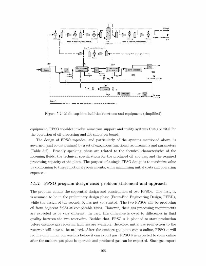
Figure 5-2: Main topsides facilities functions and equipment (simplified)
equipment, FPSO topsides involve numerous support and utility systems that are vital forthe operation of oil processing and life safety on board.
The design of FPSO topsides, and particularly of the systems mentioned above, isgoverned (and co-determines) by a set of exogenous functional requirements and parameters(Table 5.2). Broadly speaking, these are related to the chemical characteristics of theincoming fluids, the technical specifications for the produced oil and gas, and the requiredprocessing capacity of the plant. The purpose of a single FPSO design is to maximize valueby conforming to these functional requirements, while minimizing initial costs and operatingexpenses.
5.1.2 FPSO program design case: problem statement and approach
The problem entails the sequential design and construction of two FPSOs. The first, α,is assumed to be in the preliminary design phase (Front-End Engineering Design, FEED),while the design of the second, β, has not yet started. The two FPSOs will be producingoil from adjacent fields at comparable rates. However, their gas processing requirementsare expected to be very different. In part, this difference is owed to differences in fluidquality between the two reservoirs. Besides that, FPSO α is planned to start productionbefore onshore gas receiving facilities are available, therefore, initial gas re-injection to thereservoir will have to be utilized. After the onshore gas plant comes online, FPSO α willrequire only minor conversions before it can export gas. FPSO β is expected to come onlineafter the onshore gas plant is operable and produced gas can be exported. Since gas export
108

Table 5.1: Main FPSO process systems and utilities
System name Code
Crude Handling (export) 21
Architectural General - Living Quarters 1
Communication System 86
Instrument Systems 87
Jet Fuel System 61
Gas Compression incl. Cooling and Scrubbing 23
Separation and Stabilization 20
Material Handling 73
Integrated control and safety systems 70
Oily Water Treatment Systems 44
Fire Water and Foam Systems 71
Fuel Gas System 45
High Pressure Sea Water System 51
Fresh Water Systems 53
Diesel System 62
Chemical Injection Systems 42
Inert Purge System 64
Flare, Vent and Blowdown Systems 43
Seawater Systems (Low to Medium Pressure) 50
Heating Systems 41
Battery System and Uninterruptible Power Supply 85
Open Drain System 56
Compressed Air Systems 63
Main Power Generation and Distribution 13.3kV 80
Halon/CO2 Systems 72
requires much lower compression ratios than re-injection, and because of the two reservoirshave different compositions, the functional requirements for the second development areassumed to be somewhat different than fro α regarding gas handling capacity (Figure 5-3and Table 5.2).
From Figure 4, standardization appears to be a viable strategy between FPSOs α and β;all key specifications and functional requirements except three are identical at the conceptuallevel of definition. The developer’s alternative standardization strategies are broadly thefollowing:
1. Design and build both FPSOs as independent assets, with no consideration for stan-dardized systems and components among them.
2. Develop a single FPSO design that satisfies the most onerous requirements of bothFPSOs α and β. This corresponds to the “full-standardization” approach, whichprobably exploits standardization benefits the most, but also implies that one of thetwo units is greatly over-designed.
109

Table 5.2: Assumed functional requirements for FPSO α and β
Functional requirement FPSO α FPSO β0 Units
Inlet Oil Rate 275 275 mbd
Gas Lift Rate 120 45 mmscfd
Inlet Gas Rate 200 75 mmscfd
Gas Injection Rate 180 68 mmscfd
Number Of Risers 4 4 -
Export Oil Rate 100 100 mbod
Crude Quality 24 24 ◦API
Gas Injection Pressure 350 350 bara
Inlet Fluids Pressure 35 35 bara
Inlet Fluids Temperature 50 50 ◦C
Produced Water Rate 220 220 mbd
Water Injection Rate 259 259 mbd
Water Injection Pressure 225 225 bara
3. Design FPSO β so that it shares some of its components’ designs with FPSO α. Thisstrategy can be planned as a fixed commitment from the time α is designed, or in aflexible manner.
(a) A fixed-commitment strategy involves that choosing an appropriate set of com-ponents and systems on FPSO α and committing to their re-use on FPSO β.
(b) A flexible strategy involves choosing an appropriate set of components and sys-tems on FPSO α, but without committing to their re-use on FPSO β. Thedeveloper retains the flexibility to utilize as much of the existing FPSO α designas the economic and technical conditions deem appropriate at the time FPSO β
is designed. This decision will also allow consideration of design, procurement,construction and initial operation lessons learned.
Strategy 1 involves no standardization; it is the development paradigm followed in the oilproduction industry until recently. It practically ensures that both FPSOs will be optimizedaround the resources and economic conditions at the time of their development, becauseeach FPSO is optimized with no regard for future developments. Strategy 2 represents asignificant design paradigm shift, recently manifested in the oil industry with the develop-ment of series of identical facilities. It taps into benefits of standardization, such as designre-use, learning curve effects, preferred contractor agreements etc.; on the other hand, itmay imply severe standardization cost penalties compared to individually optimized FPSOsdesigned per strategy 1. Strategy 3 represents the current trend towards smart standard-ization, where the economic benefits from re-using existing, standardized designs in FPSOβ are traded-off against the benefits from fully customizing it.
110

Figure 5-3: Comparison between assumed functional requirements of FPSOs α and β
Approaches 3a and 3b are different ways of valuing smart standardization strategies,and specifically FPSO α. Approach 3a represents a “discounted-cash-flow” line of thinking,with commitment at an early date to decisions that can be postponed until later. Althoughactually doing so can be beneficial,2 it is a mistake to value the program as if it were fullyinflexible, if in reality it is not. Approach 3b is the proposed valuation paradigm, wherebyfuture decisions are modeled to be contingent on future events, and current decisions aremade based (partly) on the flexibility they create for the future.
What is the difference between strategies 1 and 3b? Both approaches suggest that designdecisions for FPSO β are made at the time FPSO β is designed, not before. The differenceis subtle, and concenrs the optimality criterion on which the design of FPSO α is based.Strategy 1 suggests the optimization of FPSO α as if it were the only development, anddoes not account the possible standardization opportunities enabled for the design of β.Approach 3b does, capturing the real opportunities created by standardization. In otherwords, the value difference between an individually optimized FPSO α according to strategy1 and an FPSO α optimized according to strategy 3b is the total value of standardization,including the value of flexibility:
[Total value createdby standardization
]=
Value of design α that wasoptimized with approach3b, as calculated withapproach 1
−
Value of design α
that was optimizedand calculated with
approach 1
What is then the value of flexibility? The answer is, the difference between the valuation
2 Committing a-priori to design decisions that can be normally postponed can be a good strategy, e.g.,
because some of the value of standardization can be transferred to the developer only if its suppliers receive
prior commitment to future orders. This effect is not considered in this work, although the proposed
methodology is perfectly capable of modeling it; see 6.
111

of an FPSO α according to approach 3b, minus its value according to approach 3a. Thisdifference is obviously due just to the fact that approach 3a ignores the future flexibilitycreated for the development of FPSO β and assumes that all decisions for both units aretaken a-priori. If there is any reason not to commit to these decisions beforehand, e.g., ifthere is any uncertainty, then delaying the decisions for FPSO β has value. This additionalvalue is captured in valuation approach 3b, but not in approach 3a.
Another way of saying the above is that the design of FPSO α creates a platform onwhich the developer can base the design of β, if it is optimal to do so in the future. Thedesign decisions for FPSO α only make it more or less likely that the established platformwill be optimally adhered to when FPSO β is developed, and the extent to which thismight happen. Therefore, the expected value of FPSO α, which is the objective of itsdesign, should also include the flexibility it creates for the organization to choose how todesign and develop FPSO β. This includes:
• The flexibility to utilize the existing design of FPSO α for FPSO β at varying degrees,i.e., re-use the design of different combinations of systems, components, and supplychain agreements.
• The flexibility to choose the timing of development of FPSO β, and the right to waitbefore finalizing the design or starting the development of FPSO β.
These decisions on alternative designs and development timing can be modeled using thegraphical modeling convention introduced in Chapter 4, as shown in Figure 5-4. Initially,the developer operates FPSO α. This state has intrinsic value due to the operating cashflows it generates. It also has value because it gives the developer the option to designany of the alternative FPSOs β1 . . . βn, each of which corresponds to a different selectionof standardized components. The developer may postpone this design decision indefinitely,i.e., never exercise the choice option at the OR node. Alternatively, the developer maydecide among β1 . . . βn, incurring design costs. In this model, it is assumed that oncemade, a design decision cannot be reversed.3 After a certain time lag that correspondsto Front-End-Engineering-Design (FEED), denoted as TtD1 . . . T tDn for each alternativeFPSO β, the developer obtains the right to begin construction of the chosen design. Afterthe “construction go-ahead,” which can also be delayed, the developer obtains the chosenFPSO βi and operates both α and βi simultaneously.
One challenge with valuing the flexibility inherent in FPSO α is the number of alternativestandardization strategies β1 . . . βn. The IDR methodology (chapter 3) is used to screenstandardization strategies for FPSO β and reduce n.
The screening of alternative standardization strategies is based on the effects on thedevelopment of FPSO β that can be measured with relative certainty from the time FPSO
3Given the long design time for such vessels, which is in the order of years, this is not a very restrictive
assumption: there is good incentive to finalize design before commencing it.
112

Figure 5-4: FPSOs α and β program development decisions
α is designed. Some of these effects involve estimates of operating cost reduction for as longas both FPSOs operate simultaneously; reduction of design and construction cost for FPSOβ; reduction of the design and construction time lag, which expedites cash flows generatedfrom the second FPSO, increasing their value. A detailed model of the effects of alternativestandardization strategies in the design and construction of FPSO β is presented in Section5.2.
Screening alternative standardization strategies so as to maximize the reduction in sparepart inventories, FEED cost and time, and construction cost and time, will produce poten-tially optimal designs fot FPSO β. This is because:
• the value of a standardized second FPSO increases monotonically as the standardiza-tion effects increase, all else being equal. For example, a shorter design time is alwaysmore valuable than a longer one. Therefore, all the standardization effects are to bemaximized.
• there is a trade-off between these standardization effects: due to technical constraints,it is impossible to increase all standardization effects simultaneously.
Therefore, the problem is to select the designs β1 . . . βn that lie on the Pareto front ofstandardized designs that maximize the effects described previously. This is done using theIDR methodology presented in Chapter 3, and presented in Section 5.3.
The final part of the methodology (Section 5.4) uses the flexibility valuation algorithmto assess the value of FPSO α that enables the design of alternatives β1 . . . βn. In a worldwithout uncertainty, it would be possible to determine from the start which of the designsβ1 . . . βn would be optimal as the second development, and consequently the value of α.This logic was captured in strategy 3a (see p.110). In the presence of uncertainties, anyof the previously identified designs β1 . . . βn may be optimal to develop in different statesof the world. The uncertainties st for this design study are assumed to be the price of oil
113

(soilt ), gas (sgas
t ) and steel (sstlt ):
st = {soilt , sgas
t , sstlt }
For example, in a state of the world of high oil or gas prices and low steel prices, a standard-ization solution that uses heavier equipment and more steel, but expedites the developmentprogram significantly might be pursued; if the reverse conditions prevail, a solution whichis slower to develop but very economic in steel may be optimal. For illustration purposes,it is assumed that the uncertainties are the price of oil, the price of gas and the price ofsteel (which in part determines the construction cost).
5.2 Standardization effects
The effects oil producing companies have so far experienced from standardization haveyielded hundreds of millions of dollars in value created. The Kizomba A and Kizomba Bdevelopments offshore Angola are a recent example of a multi-project program delivered bya “design one, build many” approach, saving some 10-15% in capital expenses (circa $400M)and 6 months in cycle time. Generally, duplication of facility designs has been found tocreate value for the second and subsequent developments in three major ways (Figure 5-5):first, capital expense (CAPEX) reduction, mainly due to repeat engineering, contracts withpreferred suppliers, discounts for material and services and integration efficiency. Secondly,value is created due to reduced operating expenses (OPEX) for the second and subsequentprojects. This is mainly due to reduced risk in start-up efficiency, improved uptime, andcommonality of spares and training. Finally, project engineers and managers use provendesigns and commissioned interfaces without “re-inventing the wheel.” Standardizationimplies reduced FEED effort requirements, fewer mistakes, increased productivity, learningetc., which in turn imply reduced cycle time. This can be extremely valuable by acceleratingthe receipt of cash flows from operations, thus increasing their value. Given a growingconcern in the oil industry about the availability of skilled human resources cycle-timeminimization becomes an even greater source of value.
Preliminary data for these effects can be found in focused studies commissioned toengineering contractors, e.g., Hyundai Heavy Industries Co. Ltd (2005) and Daewoo Ship-building & Marine Engineering Co. Ltd. (2005), or findings from oil producers’ (limited)experience with standardization; e.g., McGill & de Neufville (2005). Not surprisingly, theformer studies indicate much lower expected standardization benefits than the latter ones: acontractor publishing significant learning curve effects effectively implies that significant andcostly mistakes are made in the development of the first projects in a program. Moreover,contractors have clear disincentive to claim significant reductions in design and constructioncosts, because in an inefficient market they can claim the value created instead of passingit to the owners. As a result, even though data on standardization effects exists, it shouldbe used with scrutiny. For illustration purposes, existing data on design and construction
114

Figure 5-5: Effects of system standardization between FPSOs α and β
effects from duplicating entire FPSOs is used in this design study, with the recognition thatan accurate account of these benefits is a matter of further research.
The data on the effects of standardization in oil production projects so far applies tofully standardized projects that are based on duplicate designs (strategy 2 in page 109). Inorder to assess partial standardization strategies (according to strategy 3 in Section 5.1.2),a model is needed that helps the assessment of standardization effects given the systemsand components whose design is re-used. These effects do not only depend directly onstandardization extent (e.g,. by number of systems or by weight), because each of the mainFPSO systems has different requirements in design man-hours, equipment or bulk materialcosts and labor costs (Figure 5-6); they depend on which elements from the design of FPSOα are re-used. The purpose of this section is to provide such a model. The next paragraphsquantify partial standardization effects in the form of normalized functions. For example,the function for reduction of capital expenses for construction of the entire FPSO β wouldtake the form
CAPEX reduction for β =CAPEX for β given partial standardization with α
CAPEX β without any standardization
where the nominator represents a design where the customized components are optimized forFPSO β and the standardized ones are identical to FPSO α. The denominator represents adesign where all components are customized for FPSO β. This design, i.e., a fully customizeddesign for the second FPSO, is denoted from now on as FPSO β0.
5.2.1 Reduction in operating expenses
Evidence indicates that the simultaneous operation of two (or more) FPSOs that share stan-dardized systems and components is cheaper than what it would be if the systems shared nocommonality. This is due to reduced maintenance expenses, reduced spare part inventories,smaller need for training specialized personnel etc. The reduction in operating expenses due
115

Figure 5-6: Assumed percent breakdown of development costs by system, FPSO α
to standardization implies an increase in operating free cash flows (i.e., operating revenue -costs). The free cash flow generated from FPSO α individually can be written as
CF (xα, st) = CAP oilα soil
t + CAP gasα sgas
t − CF var(xα, st)− CF fix(xα, st)
where CAP oilα , CAP gas
α are the oil and gas production capacity of each FPSO respectively,soilt , sgas
t are the spot prices for oil and gas respectively, and CF varα ≡ CF var(xα, st) are the
variable operating costs, which correspond mainly to energy required for production. Thesecan be approximated as a fraction of P gas
α sgast because power is generated from production
gas in FPSOs such as the ones examined.
Finally, CF fixα ≡ CF fix(xα, st) denotes fixed costs, which correspond to labor, mainte-
nance and spare parts, and are the main source of benefit from standardization as far asoperating costs are concerned. Annual fixed costs are calculated as approximately 2% ofEquipment and Bulk Material Costs for each system. The fixed operating expenses for thesimultaneous operation of the same system on both FPSOs are assumed to be only half oftheir nominal value, because of shared maintenance and inventory costs (see Section 2.3).4
With these assumptions, it is possible to calculate the function g1(xα,xβ), i.e., the percent
4This number is just assumed for illustrative purposes; in a real design study it would have to be estimated
using a maintenance model. For more information and models for spare part inventory and maintenance
costs in petroleum production see the references for Section 2.3.
116

reduction in maintenance and spare part inventory costs for partially standardized FPSOs:
g1(xα,xβ) =
(1−
CF fixαβ
CF fixα + CF fix
β
)100% (5.1)
For example, consider the designs α and β0, each optimized individually around thespecifications given in Table 5.2 and Figure 5-3. Table 5.3 shows the annual maintenancecosts for each piece of equipment on each design. Consider now a design for FPSO β, inwhich only the gas compression system (system 23) is common with FPSO α. Then theannual maintenance cost for this system for both FPSOs will be only $219,810. If bothFPSOs use the system designed for FPSO β0 then the annual maintenance cost would beonly $120,400 (but the gas processing capacity of FPSO α would be severely compromised);if the two FPSOs used different systems then the annual maintenance costs would rise to$120,400 + 219,810 = $340,210. These differences in fixed maintenance costs can be usedfor the calculation of g1(xα,xβ) for each standardization solution.
Table 5.3: Assumed FPSO annual spare part costs for each system ($1,000)
System name FPSO α FPSO β0
2% of equipm. bulk 2% of equipm. bulk
Crude Handling (export) 50.73 50.73
Architectural General - Living Quarters 5.78 5.78
Communication System 5.00 5.00
Instrument Systems 11.01 10.68
Jet Fuel System 7.45 6.85
Gas Compression incl. Cooling and Scrubbing 219.81 120.30
Separation and Stabilization 869.61 787.94
Material Handling 27.23 26.51
Integrated control and safety systems 38.81 38.81
Oily Water Treatment Systems 562.74 562.75
Fire Water and Foam Systems 151.60 133.08
Fuel Gas System 9.03 8.31
High Pressure Sea Water System 95.74 17.80
Fresh Water Systems 10.45 10.45
Diesel System 7.11 6.76
Chemical Injection Systems 11.24 10.78
Inert Purge System 9.96 9.73
Flare, Vent and Blowdown Systems 21.86 16.49
Seawater Systems (Low to Medium Pressure) 109.01 23.90
Heating Systems 195.14 184.67
Battery System and Uninterruptible Power Supply 5.54 5.45
Open Drain System 67.68 59.16
Compressed Air Systems 11.01 10.68
Main Power Generation and Distribution 13.3kV 1,661.38 1,651.24
Halon/CO2 Systems 46.29 48.47
117

The function g1(xα,xβ) does not correspond directly to value created from standard-ization, it is only a factor of decrease in fixed operating expenses. The actual free cashflows generated by each FPSO are a function of the prices of oil and gas, the variable costsetc. However, it is certain that larger values of g1(xα,xβ) correspond to larger value forthe entire program, all else being equal. Therefore, the organization seeks to maximizeg1(xα,xβ) through the design of α and β.
5.2.2 Reduction in FEED cost and time
Front-end engineering design (FEED) is perhaps the phase of the development process mostaffected by a platform strategy and standardization of systems. The reasons are self-evident:FEED, involving tasks such as chemical process modeling, equipment sizing, productionschedule planning, hull design and integration planning, is mostly insensitive to the smallchanges required in (nominally) almost identical systems. So a largely standardized systemsaves the effort of preliminary design for every variant. Like in the previous section, theimpact of partial FPSO standardization on preliminary (FEED) engineering cost is modeledusing a factor g2 as follows:
Dαβ = Dβ0 [1− g2(xα,xβ)] (5.2)
where Dαβ(st) is the FEED cost of designing an FPSO β partially standardized with FPSOα, and Dβ0 is the FEED cost of designing a fully customized FPSO β0 anew.
The impact on design time can be modeled similarly:
TtDαβ(st) = TtDβ0(st)[1− g3(xα,xβ)] (5.3)
where TtDαβ(st) is the time required for the front-end design of FPSO β, given thatFPSO α is already designed, and TtDβ0 is the cost and time required for the design ofthe individually-designed, optimized FPSO β0.
Reduction in FEED cost It is customary in the design of oil exploration and productionfacilities to calculate direct design time and cost for a system in proportion to its weight(equipment and bulk). On this basis, the design cost for each system on FPSOs α andβ0 is calculated according to Berwanger (2004) as shown in Table 5.4. The FEED costsfor implementing entirely the same design on a second FPSO (100% standardization) areestimated to be around 25% of the initial FEED costs. This remaining cost is attributedto design integration, checking etc. If the second development is partially standardized, thereduction is calculated by reducing the FEED costs by 75% for each standardized system.So g2 can be written as follows:
g2(xα,xβ) = 1−Dαβ
Dβ0
=(
1−Dβ0 −∆D(xα,xβ)
Dβ0
)100%
118

where ∆D(xα,xβ) is the design cost of the standardized components if they are optimizedfor FPSO β0, minus 25% of the design cost of the respective components, if they are opti-mized for FPSO α.
For example, if FPSO α’s gas compression design (system 23 in Table 5.1, p.109) is usedwithout any alterations on FPSO β, then the FEED cost for that system is calculated as(0.25)(1, 335) = $334, 000. The design cost difference between the partially standardizedFPSO β and the individually optimized FPSO β0 is ∆D(xα,xβ) = 451− 334 = 117 (fromTable 5.4). Therefore, between two designs on that share only the design of system 23 (ifthis were possible5) the function g2(xα,xβ) that expresses standardization benefits in termsof FEED cost is calculated as
g2(xα,xβ) = 1−Dαβ
Dβ0
= 1−Dβ0 −∆D(xα,xβ)
Dβ0
= 1− 18, 011− 11718, 011
≈ 0.7%
Figure 5-7: FEED cost and time as a function of standardization by weight
Reduction in FEED time The reduction in FEED design time is modeled to be pro-portional to the reduction in FEED cost. Figure 5-7 shows how the relationship betweenthe two is found. Duplicating the design of FPSO α (i.e., fully standardizing FPSO β,point AA in Figure 5-7) costs 0.25Dα = (0.25)($20m) = $5m in FEED costs and requires0.50TtDα = (0.50)(365) = 183days in FEED time. The factors 0.25 and 0.50 representessentially cost and time experience curves in design. According to preliminary engineeringdata from Hyundai Heavy Industries Co. Ltd (2005) and Daewoo Shipbuilding & MarineEngineering Co. Ltd. (2005), the FEED design of a completely new, custom-optimizedFPSO β0 costs Dβ0 = $18.011m and requires TtDβ0 = 328 days (point AB0 in Figure 5-7).
5Standardizing only this system will rarely be possible because of the couplings between systems on the
FPSO. So the calculation of g2(xα,xβ) shown here is essentially the marginal contribution of standardizing
system 23 when no other system is standardized.
119

This implies that the opportunity FEED cost per day for standardization is constant, andequal to
c =Dβ0 − 0.25Dα
TtDβ0 − 0.50TtDα=
18.011− 5.000328− 183
≈ $90, 000/day
Table 5.4: Assumed FPSO FEED costs for each system ($1,000)
System name FPSO α FPSO β0
Crude Handling (export) 136.4 136.4
Architectural General - Living Quarters 1190.0 1190.0
Communication System 3.6 3.6
Instrument Systems 40.5 40.5
Jet Fuel System 95.2 95.2
Gas Compression incl. Cooling and Scrubbing 1335.9 451.7
Separation and Stabilization 6173.7 5579.9
Material Handling 288.5 287.0
Integrated control and safety systems 42.8 42.8
Oily Water Treatment Systems 1669.6 1669.6
Fire Water and Foam Systems 178.0 175.4
Fuel Gas System 91.2 90.7
High Pressure Sea Water System 0.0 0.0
Fresh Water Systems 0.0 0.0
Diesel System 1.4 1.4
Chemical Injection Systems 14.3 14.3
Inert Purge System 24.3 24.3
Flare, Vent and Blowdown Systems 591.0 446.5
Seawater Systems (Low to Medium Pressure) 0.0 0.0
Heating Systems 2365.0 2172.2
Battery System and Uninterruptible Power Supply 26.8 26.4
Open Drain System 27.4 27.4
Compressed Air Systems 40.5 40.5
Main Power Generation and Distribution 13.3kV 5644.8 5604.2
Halon/CO2 Systems 19.3 19.0
Based on Figure 5-7, the required FEED time for a partially standardized FPSO β canthen be calculated as
TtDαβ = TtDβ0 − c−1∆D(xα,xβ)
To see this, notice that if the difference in design cost ∆D(xα,xβ) is zero, then TtDβ =TtDβ0 : FPSO β is identical to β0; if ∆D = TtDβ0 − 0.50TtDα then FPSO β is identical toFPSO α, exploiting fully the reduction in FEED time due to standardization. The function
120

g3(xα,xβ) can be written as
TtDαβ = TtDβ0 [1− g3(xα,xβ)]⇒ g3(xα,xβ) = 1− TtDαβ/T tDβ0
⇒ g3(xα,xβ) = 1− TtDβ0−c−1∆D(xα,xβ)
TtDβ0
⇒ g3(xα,xβ) =(
∆D(xα,xβ)cT tDβ0
)100%
(5.4)
5.2.3 Reduction in construction cost
Construction costs include labor cost of equipment and bulk as well as an overhead (e.g.,project management, detailed engineering, construction supervision, procurement services,inspection etc.). Hyundai Heavy Industries Co. Ltd (2005) and Daewoo Shipbuilding &Marine Engineering Co. Ltd. (2005) provide estimations for these learning curve effects fora series of identical FPSO topsides manufactured in a row as shown in Figure 5-8. The totalconstruction cost reduction for duplicating an existing FPSO (by the same contractor withina reasonable amount of time from the first development) is potentially 2% for material andbulk, and 10% on average for labor (engineering, fabrication etc.). As discussed above, thisdata is expected to predict smaller effects than the industry averages (e.g., as reported byNASA in Table 2.1, p. 31).
Construction cost is assumed not to be deterministically known, but also significantlyaffected by uncertain factors, such as the price of steel. This dependency is captured hereby writing Cαβ(st) to denote the construction cost of a partially standardized FPSO β
given the existence of FPSO α already, and Cβ0(st) the construction cost of an individuallyoptimized FPSO β0. Then the construction cost reduction for the second FPSO due topartial standardization with the first is denoted g4 (percent), and written as
Cαβ(st) = Cβ0(st)[1− g4(xα,xβ)] (5.5)
For the purpose of this design study, the impact of steel price on the construction cost wastaken to be linear, affecting the “Equipment Material” and “Bulk Material” cost items only.
To estimate the function g4(xα,xβ) cost savings or increases can be apportioned toindividual standardized systems assuming these learning curve effects apply to each systemseparately. For example, the construction cost of system 23, Gas Compression, Cooling andScrubbing, can be estimated for FPSO α as (2, 788.8+1, 607.3)+ (155.1+1, 953.4) = 6, 504(Table 5.5). If the same design is used in FPSO β, the cost for system 23 in β can be $298,000cheaper, calculated as 6, 504− (2, 788.8 + 1, 607.3)(0.98) + (155.1 + 1, 953.4)(0.90) = 298. Ifthis system had been customized for FPSO β (as assumed in the design β0) then its totalcost would be (1, 744.1 + 73.3) + (663.2 + 806.0) = 3, 285 (from Table 5.6). Denoting thedifference ∆C(xα,xβ) = 3, 285− 6, 206 = −2, 921 shows that re-using the design of system23 from FPSO α on FPSO β incurs a “standardization penalty,” because of over-sizing theequipment above its required capacity. This penalty is larger than the learning curve effects
121

Figure 5-8: Assumed learning curves in FPSO construction costs
that make the second instance of system 23 cheaper than the first by $298,000. If only thissystem were standardized between FPSOs α and β, the corresponding g4 function wouldread
g4(xα,xβ) = 1− Cαβ(st)Cβ0
(st)
= 1− Cβ0(st)−∆C(xα,xβ)
Cβ0(st)
= 1− 103,039−3,285+6,206103,039 = −2.8%
i.e., around a 3% cost increase.
5.2.4 Reduction in construction time
A typical schedule of construction activities for an FPSO includes 3 major phases: pre-fabrication design (i.e., detailed and construction design), system fabrication and systeminstallation and integration. For the last phase, installation and integration, the schedulereduction is assumed in this analysis to be negligible.6 For the other two phases, thereduction in construction schedule for a fully standardized second FPSO is extracted fromexisting assumed data and allocated to individual systems.
Reduction in detailed and construction design time is nominally around 50% for afully-standardized second development, and is apportioned to individual systems dependingon their contribution to the total construction cost. Considering that detailed/constructiondesign costs account for approximately 14.5% of the total construction costs; total construc-tion cost is $103.039m for FPSO β0 and $114.344m for FPSO α; and FPSO β0 requires
6One justification for this is that integration benefits are realized only if there are no customized compo-
nents.
122

Table 5.5: Assumed FPSO α construction costs for each system ($1,000)
Equipment Equipment Bulk Bulk
Material Labor Material Labor
cost cost cost cost
System name ($1,000) ($1,000) ($1,000) ($1,000)
Crude Handling (export) 554.98 24.14 459.55 458.81
Architectural General - Living Quarters 50.00 50.00 0.00 0.00
Communication System 100.00 0.00 0.00 0.00
Instrument Systems 134.76 7.65 85.43 105.32
Jet Fuel System 40.00 5.00 120.00 0.00
Gas Compression incl. Cooling and Scrubbing 2788.83 155.06 1607.33 1953.36
Separation and Stabilization 6164.66 351.08 11227.56 14127.68
Material Handling 530.91 42.98 13.60 19.37
Integrated control and safety systems 752.00 7.20 24.25 60.12
Oily Water Treatment Systems 8606.91 315.67 2647.99 3200.94
Fire Water and Foam Systems 1774.36 36.28 1257.54 1821.77
Fuel Gas System 40.64 2.46 140.05 167.14
High Pressure Sea Water System 300.67 12.74 1879.58 0.00
Fresh Water Systems 200.00 25.00 1378.00 0.00
Diesel System 2.22 0.29 139.90 181.66
Chemical Injection Systems 81.14 2.72 143.73 74.46
Inert Purge System 131.15 4.59 68.09 81.49
Flare, Vent and Blowdown Systems 205.44 70.67 231.79 276.64
Seawater Systems (Low to Medium Pressure) 300.67 12.74 1879.58 2245.71
Heating Systems 1506.95 259.55 2395.76 3004.25
Battery System and Uninterruptible Power Supply 108.67 1.97 2.05 2.03
Open Drain System 57.06 5.18 1296.49 1547.01
Compressed Air Systems 134.76 7.65 85.43 105.32
Main Power Generation and Distribution 13.3kV 32612.09 590.44 615.49 610.11
Halon/CO2 Systems 541.80 11.08 383.99 556.28
123

Table 5.6: Assumed FPSO β construction costs for each system ($1,000)
Equipment Equipment Bulk Bulk
Material Labor Material Labor
cost cost cost cost
System name ($1,000) ($1,000) ($1,000) ($1,000)
Crude Handling (export) 554.98 24.14 459.55 458.81
Architectural General - Living Quarters 50.00 50.00 0.00 0.00
Communication System 100.00 0.00 0.00 0.00
Instrument Systems 135.23 7.65 78.35 96.40
Jet Fuel System 40.00 5.00 120.00 0.00
Gas Compression incl. Cooling and Scrubbing 1744.12 73.28 663.20 805.98
Separation and Stabilization 5612.30 318.44 10146.47 12765.70
Material Handling 516.94 41.90 13.34 18.99
Integrated control and safety systems 752.00 7.20 24.25 60.12
Oily Water Treatment Systems 8606.93 315.68 2648.01 3200.97
Fire Water and Foam Systems 1465.39 33.10 1196.12 1735.75
Fuel Gas System 35.30 1.81 130.88 156.17
High Pressure Sea Water System 300.67 12.74 1879.58 0.00
Fresh Water Systems 200.00 25.00 1378.00 0.00
Diesel System 2.22 0.29 133.02 173.45
Chemical Injection Systems 81.14 2.72 134.45 70.11
Inert Purge System 131.15 4.59 63.53 76.04
Flare, Vent and Blowdown Systems 160.02 56.11 169.68 202.50
Seawater Systems (Low to Medium Pressure) 0.00 0.00 478.02 570.97
Heating Systems 1464.09 240.76 2229.33 2795.09
Battery System and Uninterruptible Power Supply 107.06 1.94 2.02 2.00
Open Drain System 57.06 5.18 1126.19 1343.87
Compressed Air Systems 135.23 7.65 78.35 96.40
Main Power Generation and Distribution 13.3kV 32412.99 586.83 611.74 606.38
Halon/CO2 Systems 533.70 12.06 435.63 632.16
124

around 243 days in detailed design versus 260 for FPSO α, the opportunity cost of stan-dardization for construction is estimated as in Section 5.2.2 as
c′ =0.145 [103.039− (0.50)(114.344)]
243− 130≈ $58, 000/day
The required detailed design time for a partially standardized FPSO β, TDDβ,α , is then
TDDαβ = TDD
β0− (c′)−1∆C(xα,xβ)
Where TDDβ0
is the detailed design time required for an individually optimized FPSO β0.For example, the detail design time saved by re-using only system 23 in FPSO β can beestimated as (0.145)(2, 921)/58 ≈ 7 days.
Reduction in fabrication time is estimated individually for each system to be around2% for the second FPSO. The impact of such a reduction is then calculated based on thefabrication and installation schedule. Essentially, if the fabrication of a system on thecritical path is expedited, then the overall fabrication schedule is shortened; if not, thefabrication schedule is unaffected. Consider again system 23: For the first FPSO, system23 requires 250 days fabrication time. A 2% reduction in fabrication time corresponds to5 days, which does not affect the FPSO delivery schedule at all (Figure 5-9). The totalreduction in construction time for system 23, including detailed design and fabrication, willbe 7 + 5 = 55 days, of which only 7 will be actually materialized (if only system 23 isstandardized). On the other hand, combined with other fabrication time reductions, theremaining 5 days may be important. To capture these effects, the construction schedule issolved for each standardization strategy.
Figure 5-9: FPSO α construction schedule. All links are start-to-start with lag.
125

5.3 Screening of platform strategies
The next step after quantifying the measurable effects of partially standardizing FPSO β, isto screen standardization strategies between FPSOs α and β that maximize the associatedbenefits. This is done as described in chapter 3, by first building an SDSM representativeof a “base” design x∗ and then explore how removing “sensitivities,” i.e., SDSM entries,increases the set of systems that can potentially be standardized among designs x and xα
and among designs x∗ and xβ. As shown in chapter 3, it will then be possible to standardizethese systems among FPSOs α and β as well.
For this design study, the SDSM was built considering the design of FPSO α, (Figure5-10)7 i.e.,
x∗ ≡ xα
Identifying FPSO α as the base design is not necessary but implies that for this analysisFPSO α is optimized according to strategy 1 (see p.109), and the standardization strategiesexplored correspond to any standardization opportunities that can be salvaged for FPSO β.Taking x∗ 6= xα would imply that both FPSOs α and β can be optimized simultaneouslyso as to maximize the value of the entire program (strategy 3a).
5.3.1 The low-hanging fruit
Some sets of systems will be generally decoupled from other systems even before any sen-sitivities are removed from the SDSM. These are the systems that can be standardizedbetween FPSOs α and β anyway, i.e., the “low-hanging fruit.” If they are not standardizedin reality, this may be for non-technical reasons that make their customization optimal ina larger business context.
These standardization opportunities can be easily identified with a direct application ofthe IDR algorithm to FPSO α’s SDSM. The result is shown in Figure 5-11. The selectionof standardized systems is intuitive with the imposed changes in functional requirements.It involves systems that are completely irrelevant to the production facilities (such as livingquarters), or systems that are uncoupled with the changes in functional requirements (suchas systems related to oil processing).
5.3.2 Compromise strategies
In general, standardization requires compromise, because systems and components are nor-mally designed to exactly match the specification requirements imposed by other compo-nents they are coupled with. Removing SDSM entries requires that these couplings arebroken, i.e., that “slack” is added to the design of systems and components.8 In principle,
7This cannot be inferred from any data appearing here. It is a matter of convention and agreement
among the members of the multi-disciplinary team that models the SDSM.8In this design study, all compromise is required only of the designers of FPSO β, since the original SDSM
corresponds exactly to FPSO α. Given the differences in functional requirements prescribed in the outset
126

Figure 5-10: Original SDSM for FPSO α
Figure 5-11: Partitioned SDSM for FPSO α, showing standardized systems according tostrategy 0 (no entries removed).
127

the local “slack” imposed on the design of individual systems should be minimized; therefore,standardization strategies should be explored that minimize the number of SDSM entriesremoved. Equivalently, the maximum number of standardized components for a given num-ber of entries removed should be sought. This is achieved using the IDR algorithm foralternative combinations of SDSM entries removed.
At the same time, standardization strategies should aim at maximizing value. Given thatthe value of all the alternative strategies that may be chosen when FPSO β is developeddepend on the uncertainties at that time, so are unknown beforehand, standardizationstrategies should be screened for the closest proxies for value that do not depend on uncertainparameters (see Section 5.3). These are the strategies that maximize the functions g1 . . . g5.Therefore, screening alternative standardization strategies for FPSO β amounts to findingthe Pareto front of standardization strategies that maximize functions g1 . . . g5.
Finding these points is formally a multi-objective optimization problem on a 5-dimensionalPareto front.9 These Pareto fronts are shown pair-wise in the matrix of plots in Figure 5-12.Each plot shows 2000 simulated standardization strategies. Each point on the plots, i.e.,each strategy, was obtained by randomly removing entries from the “customized systems”quadrant of the SDSM in Figure 5-11 (i.e., the south-east quadrant), running the IDR algo-rithm on the resulting matrix, and calculating functions g1 . . . g5 for the set of standardizedsystems. The plots show 165 non-dominated solutions, shown as black squares instead ofgrey circles, i.e., strategies for which any improvement to one of the objectives implies adeterioration of another objective.10 Notice that most of these strategies are very similar,s they can be grouped in a smaller number of representative standardization alternatives.For illustration, 16 strategies (out of 165) were selected, and the values of the functionsg1 . . . g5 corresponding to each are shown in Table 5.7.
The plots in Figure 5-12 are rich in qualitative and quantitative information on alterna-tive standardization opportunities. The plots of g2 against g3 and g4 against g5 show a clearlinear relationship between the two metrics. This is not surprising in this case, since theirrelationship was modeled to be linear (equations 5.2 and 5.4, and Sections 5.2.3 and 5.2.4).This implies no trade-off between these effects. Moreover, the percent-wise standardizationeffect on construction time (corresponding to detailed design and fabrication) is negligibleaccording to the range of g5: all alternatives provide a reduction of about 5%. Whilst thiscan be a significant and valuable reduction in construction time, it does not vary much be-tween alternative strategies. This indication could be used to drop this screening criterionaltogether, narrowing down the dominant standardization strategies. Finally, the plots in
(see Figure 5-3), this is not unreasonable: it broadly implies that the gas handling system will be optimized
for FPSO α to accommodate the higher capacity requirements, and then it may be utilized on FPSO β as
well, if the standardization benefits at the time justify it.9In this work, the design space was searched using Monte-Carlo simulation, and not optimization.
10On a two-dimensional Pareto plot, the Pareto-optimal points usually lie on an “edge” of the set all the
points in the plot; here, they do not. This is because the Pareto-front is 5-dimensional, so a point that seems
“in the middle” of others in one plot, is on the edge of the region of points on another plot.
128

Figure 5-12: 2000 standardization strategies (produced with Monte-Carlo simulation).Black square markers show the Pareto-optimal strategies. Y-axes and x-axes on off-diagonalplots are % benefit for the g functions.
Figure 5-12 indicate a trade-off between capital cost reduction for FPSO β, i.e., g2 and theother standardization effects: re-using the design of a system from FPSO α means that itwill be oversized for FPSO β.
5.4 Valuation of standardization program
The application of the IDR methodology achieved screening the design space for standard-ization of FPSO β from 238 to 16 representative Pareto-optimal strategies that maximizemeasurable effects on design and construction cost and time, and operational expenses.The program’s flexibility is that each of these 16 alternatives might be optimally developedin a certain future state of the world. To make the presentation more tractable, the 16strategies are screened further down to 5, picked manually using the data in Table 5.7 tobe representative of the Pareto fronts in Figure 5-12. These are strategies 1, 2, 9, 13 and14, and are shown in Table 5.8.
The flexibility valuation methodology introduced in Chapter 4 is used on these 5 alter-natives to estimate the value of the program starting with FPSO α (Figure 5-13). Basedon the model in chapter 4, the expected value of each state of owning and operating FPSOs
129

Table 5.7: Measurable standardization effects: g(%) functions for β1 . . . β16
Strategy g1 g2 g3 g4 g5 Strategy g1 g2 g3 g4 g5
β1 47.43 70.08 42.7 -0.22 4.46 β9 34.18 46.84 28.54 1.18 4.47
β2 52.04 72.43 44.13 -6.23 4.45 β10 48.17 63.72 38.82 -3.17 4.46
β3 51.76 70.79 43.13 -6.08 4.45 β11 50.51 72.38 44.1 -3.2 4.46
β4 45.55 70.83 43.16 -0.16 4.47 β12 51.89 72.38 44.1 -6.23 4.45
β5 36.39 49.21 29.98 0.83 4.47 β13 36.52 47.89 29.18 0.98 4.47
β6 47.85 71.79 43.74 -0.37 4.46 β14 47.85 71.79 43.74 -0.37 4.46
β7 51.89 72.38 44.1 -6.23 4.45 β15 51.76 70.79 43.13 -6.08 4.45
β8 45.51 69.36 42.26 -0.01 4.47 β16 52.04 72.43 44.13 -6.23 4.45
Figure 5-13: FPSOs α and β program development decisions
β1, β2, β9, β13, β14 is given by equation 4.2, re-written below.
E [Vα(s0)] =T∑
t=t0
e−rαtE[CF (xα, st)] (5.6)
E [Vαβi(s0)] =
T∑t=t0
e−ritE[CFi(st)] for i = 1, 2, 9, 13, 14 (5.7)
where ri is an appropriate discount rate for each combination of assets αβi; CFi(st) isthe per-period cash flow generated by operation of asset α and βi simultaneously; rα isthe appropriate discount rate for FPSO α; and CF (xα, st) is the cash flow generated byoperation of FPSO α alone.
The timing options to construct each of β1, β2, β9, β13, β14 are written according to equa-tion 4.3 as
Fαβi(st) = max
[Iαβi
(st), e−rαiδtE[Fαβi(st+δt)
]for i = 1, 2, 9, 13, 14 (5.8)
where Fαβi(st) denotes the value of the option to construct βi; Iαβi
(st) is the intrinsic valueof this option, i.e., the value of immediate exercise; rαi is an appropriate discount rate for
130

Table 5.8: Standardization strategies: standardized systems between FPSOs α and β (5selected strategies)
System name β1 β2 β9 β13 β14
Crude Handling (export) • • • • •Architectural General - Living Quarters • • • • •Communication System • • • • •Instrument Systems • • • • •Jet Fuel System • • • • •Gas Compression incl. Cooling and Scrubbing •Separation and Stabilization • • •Material Handling • • • • •Integrated control and safety systems • • • • •Oily Water Treatment Systems • • • • •Fire Water and Foam Systems • • • •Fuel Gas System • • • • •High Pressure Sea Water System • • • •Fresh Water Systems • • • • •Diesel System • • • • •Chemical Injection Systems • • •Inert Purge System • • • •Flare, Vent and Blowdown Systems • •Seawater Systems (Low to Medium Pressure) •Heating Systems • • • • •Battery System and Uninterruptible Power Supply • • • • •Open Drain System • • • • •Compressed Air Systems • • • •Main Power Generation and Distribution 13.3kV • • • • •Halon/CO2 Systems • • • • •
risk in the future value of the option to transition from a state of operating FPSO α tooperating α and βi simultaneously.
Given the construction time lag, the value of immediate exercise of this option is givenaccording to equation 4.5, re-written below for the construction of βi
Iαβi(st) = e−riTtBiE [Vαβi
(st+ttb)]− e−rαTtBiE [Vα(st+TtB)]− e−rcTtBiE[Cαβi
]
(5.9)
where rc denotes an appropriate discount rate for the construction cost risk.Finally, the value of the choice option among the 5 different designs is written according
to equation 4.6
OR(st) = max [ maxi
(e−rFiTtDiE[Fαβi
(st+TtDi)]− e−rf TtDiDi
),
e−rORδtE[OR(st+δt)](5.10)
131

Table 5.9: Estimated costs for 5 selected standardization programs (based on current pricesof oil, gas and steel).
Annual spares FEED cost FEED Constr. cost Constr.
State cost $1,000 $1,000 time, days $1,000 time, days
αβ0 3,771 18,139 330 103,039 554
αβ1 1,982 5,427 189 103,263 529
αβ2 1,808 5,000 184 109,456 529
αβ9 2,482 9,643 236 101,820 529
αβ13 2,394 9,452 234 102,032 529
αβ14 1,966 5,117 186 103,417 529
where rFi, i = 1, 2, 9, 13, 14 denotes an appropriate discount rate for the future value of theconstruction option, Fαβi
, obtained by design.Even though notation becomes unwieldy, the essence of equations 5.6 to 5.10 is simple.
They represent a system to be solved recursively for various future values of the uncer-tainties. This system is constructed by simply combining the equations that represent the“option building blocks” introduced in 4.2, so that they correspond to the developmentdecisions shown in Figure 5-13. They are solved using the valuation methodology presentedin Section 4.3.
The uncertainties st for this design study are assumed to be the price of oil (soilt ), gas
(sgast ) and steel (sstl
t ), with “current” values taken to be representative of the market late2005,
{soil0 , sgas
0 , sstl0 } = {56, 9, 143} ($/bbl, $/mscf, $/ton)
and expected growth rates equal to {0.12, 0.10, 0.06} respectively. The covariance matrixof the three factors was estimated based on annual data over the past 20 years:
COV AR =
0.0289 0.0429 0.00260.0429 0.1467 0.01900.0026 0.0190 0.0463
5.4.1 Valuation results
Equations 5.6, 5.7, 5.8, 5.9 and 5.10 are solved in reverse order twice:11 once, using thevaluation algorithm introduced in Chapter 4 with the risk-adjusted expected growth ratesfor the underlying uncertainties; and a second time using the risk-neutral dynamics for thesame factors, i.e., assuming that they grow at the risk-free rate. The two sets of resultsshould be different, since the values of the two phases of development (FPSO α and FPSO α
11Both solutions used the same 50, 000 paths and 10, 000 paths per bin on average along each dimension.
The planning horizon was taken to be 10 years and the time increment 1 year. The risk-free rate was assumed
rf = 5%.
132

and β together) are not perfectly correlated because only FPSO β produces gas. Assumingthat the assumptions underlying risk-neutral valuation hold for these uncertain factors,the second valuation should be considered formally correct. However, if both valuationmethodologies indicate that the same standardization alternative for FPSO β should bepursued and if they rank the design solutions the same way, then the risk-neutral valuationand the proposed methodology are equivalent for design purposes.
First, the value of the future cash flows of state α is calculated, given an assumedaccepted discount rate rα = 20%. Then the value of each of the states β1, β2, β9, β13, β14
is found for each representative vector of the uncertainties at each time, by varying therisk compensation depending on the risk in future values. These values are shown in Table5.10 as Vαβ , and their differences are due to the differences in fixed operating expenses foreach FPSO β. The timing options to develop each of the FPSOs β1, β2, β9, β13, β14 based onFPSO α are calculated using equation 5.8, and are shown in Table 5.10 as Fαβ . These valuesinclude the differences between β1, β2, β9, β13, β14 in construction cost and time. Notice inTable 5.10 that both the risk-adjusted and the risk-neutral valuation rank the alternativestrategies the same way.
Table 5.10: Value of states αβi
Vαβ Vαβ
Assets risk-neutral risk-adjusted
α 8,638,000 10,067,000
αβ1 24,998,000 27,361,000
αβ2 25,018,000 27,380,000
αβ9 24,943,000 27,305,000
αβ13 24,953,000 27,315,000
αβ14 25,000,000 27,362,000
The timing options are valued accordingly, and the risk-neutral and risk-adjusted re-sults are compared in Table 5.11. Again, notice that both valuation methodologies rankalternative standardization strategies the same way.
Table 5.11: Value of construction options for states αβi
Fαβ Fαβ
Assets risk-neutral risk-adjusted
αβ1 11,156,000 10,485,000
αβ2 11,168,000 10,494,000
αβ9 11,121,000 10,460,000
αβ13 11,127,000 10,464,000
αβ14 11,157,000 10,486,000
133

The value of the choice option associated with state α is calculated using equation 5.10,and found equal to OR = 9, 311, 000 using risk-neutral valuation and OR = 8, 849, 000using real-world dynamics. This value corresponds to the value of strategy 3b (p. 110),whereby the standardization decision is made at the point FPSO β is developed. This valueis inherent to the value of the entire program, i.e., FPSO α as of the time of the valuation.The net present value of the program, and thus the criterion for the design of FPSO α, isthe value of the choice option, plus the value of its intrinsic cash flows (Table 5.10), less theconstruction costs for FPSO α.
To isolate the value of flexibility to choose standardization strategies, an additionalanalysis is performed. The value of the compound option is calculated, to first designand then construct each of β1, β2, β9, β13, β14, without the flexibility to choose amongstthem. The results are shown in Table 5.12. The value of each of these options correspondsto “committing” strategies 3a. Observe that the value of the choice option found above,OR = 9, 311, 000 (or OR = 8, 849, 000), is equal to the value of the option to developstandardization alternative β16. This implies that the option to defer the choice of stan-dardization alternative, i.e., the difference between strategies 3a and 3b, is zero, and thatselection, design and development of FPSO β is immediately exercised.
Table 5.12: Option to design and develop states αβi
ORαβ ORαβ
Assets risk-neutral risk-adjusted
β1 7,853,000 7,458,000
β2 7,725,000 7,334,000
β9 9,311,000 8,849,000
β13 9,244,000 8,784,000
β14 7,755,000 7,364,000
5.5 Summary
This chapter presented an application of the methodologies proposed in this thesis to thedesign of programs of two sequential Floating Production, Storage and Offloading (FPSO)units. The purpose of this study was to demonstrate the calculation of value added to theentire program, by the opportunity to base the design of select systems in the second asseton the existing designs of the first. In principle, this value has a flexibility component,stemming from the fact that the choice of alternative standardization design can be delayeduntil the second asset is designed.
The two-step methodology was used for the screening and valuation of the flexibility andreal options embedded in the program. The screening of alternative second-phase designswas based on the estimated reduction in design and construction cycle time, the estimated
134

effect on design and construction costs, and the reduction on fixed operating expensesfor the program; i.e., screening was based on measurable effects at the time of the firstdevelopment. This screening resulted in 165 Pareto-optimal standardization alternatives,obtained using Monte-Carlo simulation. Valuation was performed on only 5 of these 165alternative designs for illustrative purposes. It was found that for the particular data,which was partly real and partly modified, the flexibility to delay the design decision forthe second FPSO was not valuable, because the second development was optimally designedand developed immediately. On the other hand, it was shown that for this design study,the valuation based on the proposed methodology indicates the correct design alternative,despite the fact that it is wrong from a diversified investor’s viewpoint.
135

136

Chapter 6
Conclusions and future work
6.1 Summary
This thesis introduces a framework and methodologies that enable engineering managementteams to assess the value of flexibility in programs of standardized systems, thus bridginga gap in the literature and practice between platform design and design for flexibility,particularly for large-scale, capital intensive systems implemented only a few times overthe medium term. The main hypothesis for this work is that platform design creates anddestroys future flexibility at the same time and in different ways, so the two paradigmscan be competing in some ways and complementary in others. Therefore, the need wasidentified for a structured process that enables the practical simultaneous consideration forplatform and flexibility design. The need for such a process is driven by the high potentialvalue of both platforms and flexibility.
The approach taken in this thesis follows a two-step rationale: first, one must framethe flexibility one perceives to have available to them for the future, i.e., express their “realoptions” for expanding, contracting, improving or otherwise modifying an existing system.The second step is to value the existing design, considering how much flexibility it allows forthese modifications. In the context of standardization in large-scale systems, the evolutionof a program of projects is perceived as the design and development of a new asset whichis partially standardized with existing systems in place.
The two-step rationale is not novel per-se. The contribution of this work lies in improvingthis two-step process in a structured and systematic way that enables the exploration ofplatform design opportunities and flexibility for programs of large-scale systems. Platformdesign in large-scale projects is inherently a multi-disciplinary effort, subject to multipleuncertainties and qualitative and quantitative external inputs. To the best of the author’sknowledge, no such design management methodology exists to date, that is (a) suitable forlarge-scale, complex projects; (b) modular, with modules that are based on proven conceptsand practices; (c) open to inter-disciplinary and qualitative expert opinion; (d) is effectivelya basis for communication between the traditionally distinct disciplines of engineering and
137

finance.
To this end, this thesis made three contributions:
• A novel, inter-disciplinary methodology and algorithm for screening potential stan-dardization alternatives at various levels of system aggregation. Because it identi-fies the standardized system components that should determine the design of thecustomized ones, that are insensitive to changes in functional requirements betweenvariants, the methodology is called Invariant Design Rules (IDR).
• A graphical representation of common decisions in engineering design and develop-ment, and a one-to-one correspondence of these decisions to real option formulations.For the solution of the model, a simulation-based real options valuation algorithmfor these decisions is developed. The algorithm involves simulation of the real-worldprobability dynamics of multiple uncertainties and invokes equilibrium, rather thanno-arbitrage arguments for options pricing. The practical contribution of this method-ology is potentially very significant: the methodology and algorithm offer solutions tothe major impediments to widespread use of real options theory in engineering designapplications, i.e., lack of an unambiguous modeling language, and the no-arbitrageprinciples.
• Finally, this thesis demonstrated a use of the developed methodologies in an FPSOdesign study. The contribution lies in a subtlety: whereas existing screening method-ologies rely on criteria that depend on future uncertainty, the methodology presentedin chapter CH5 does not. Instead, it screens potential future standardized devel-opments based on criteria that are measurable as of the time of the screening. Asa result, each of the alternative second-phase standardization strategies (denoted asFPSOs β13, β24 . . . β67 in chapter 5) will surely be the optimal strategy in some futurestate of the world. The flexibility created by the first FPSO design is the abilityto choose from these standardization strategies later, depending on how uncertaintyunfolds.
6.2 Future research
This work can be extended in many directions, some of more academic interest and othersof more practical value. On a practical level, the valuation methodology can be used as anobjective function for the optimization of the entire program. As another application, thetwo-step methodology can be used to trade-off a-priori commitment with future flexibility ina program of projects (see footnote 2, p. 111). Possible extensions to the IDR methodologyrelate to its being used to guide the automatic selection of standardization alternatives.These future research directions are examined next.
138

6.2.1 Flexibility-based optimization and value created
Recall Section 5.1.2, p.108, and the analysis on alternative program development stan-dardization strategies. A distinction was drawn among a strategy of no standardization(strategy 1, ensuring that both FPSOs are optimized around the conditions at the time oftheir development), and a strategy of smart standardization (strategy 3), where the eco-nomic benefits from re-using existing designs are traded-off against the benefits from fullcustomization. The latter strategy could be planned either as a prior commitment as towhich ones the standardized components may be (approach 3a), or with flexibility, wherethe standardization decision is made when the second asset is developed (approach 3b).
The difference between approaches 1 and 3b is subtle. Strategy 1 implies the opti-mization of the first asset without consideration for possible expansion with the second.According to approach 3b, the first asset is designed in anticipation of the second. Theirdifference is the total value that can be created by standardization. An interesting questionconcerns the value of flexibility that can be created by standardization. Specifically,
Assuming that the set of alternative standardization choices available to the
designers of β can be significantly affected by the design of α, how much value
from flexibility can the developer create by using approach 3b (instead of 1) to
optimize FPSO α?
The value of flexibility of a design optimized according to approach 3b is V3b(α3b) −V3a(α3b); the value of flexibility of a design optimized using approach 1 is V3b(α1)−V3a(α1).The value of flexibility created by optimizing α with a valuation method that accounts forflexibility (e.g., approach 3b) is the difference between these two quantities:
Value of flexibility created = [V3b(α3b)− V3a(α3b)]− [V3b(α1)− V3a(α1)]
If this difference is larger than the apparent the penalty in FPSO α because it is notoptimized individually, i.e., the difference
Apparent standardization penalty for FPSO α = V1(α1)− V1(α3b)
then the developer using approach 1 to develop and value FPSO designs is forfeiting valueof flexibility. In other words, not only does approach 1 not give the correct value of FPSOα, it also leads to suboptimal design decisions.
A proposed extension of this research, and a way to potentially change the prevalentdesign paradigm so that it considers flexibility, is to apply this simple arithmetic to existingcase studies. This can serve to demonstrate in a systematic way, how much value is forfeitedin current practice because flexibility is not considered.
6.2.2 IDR-based platform optimization
Section 2.4 explained that the selection of platform components in a system of n distinctmodules is a combinatorial problem of size 2n, and the recent focus of interesting research.
139

Specifically, Simpson & D’Souza (2002) and Simpson & D’Souza (2003) propose the opti-mization of platform architectures and variants in a single stage using genetic algorithms.The genome in the genetic algorithm codifies the design variables for each variant in theproduct family, and includes a “control vector” of ones and zeros, equal to the length of thedesign vector for each variant. The control vector indicates whether each design variable isshared among variants, and invokes corresponding constraints in the system model.
This approach has two problems. Firstly, it runs the risk of indicating that platformcomponents are variables “belonging” to very different physical components of the system.Secondly, it makes no use of technical or constraint information from the technical modelof the variants; in effect, the algorithm searches the entire combinatorial space of potentialplatforms.
As an extension to the platform optimization literature, the IDR algorithm can becoupled with the genetic algorithm proposed by Simpson & D’Souza (2003) to narrow downthe search of alternative platform strategies. If derivative information is also available fromthe system model, the SDSM can also be calculated automatically, minimizing the need forengineering input.
6.2.3 Application: trading-off commitment and flexibility
In many practical contexts, including FPSO program design to a certain extent, the designstudy presented in Chapter 5 is contrived, mainly by assuming that benefits can be realizedfor the second development, even if there has been no prior commitment to standardization.In reality, committing a-priori to design decisions that can be normally postponed can be agood strategy, e.g., because some of the value of standardization can be transferred to thedeveloper only if its suppliers receive prior guarantee of future orders. Therefore, there isa trade-off between commitment to a standardized strategy (which yields standardizationbenefits) and flexibility to choose standardization strategies in the future.
This trade-off is often captured in option-like contract clauses between the developerand suppliers. Effectively, these clauses swap a fixed “large-quantity” discount for advanceorders, against the expected losses to the supplier if the developer does not follow upwith the standardization strategy. This trade-off is of great practical interest to large-scale development organizations, because it allows them to consider not only technical andeconomic performance, but also supply chain and organizational issues that drive programdevelopment decisions. The framework presented in this thesis can be extended in thisdirection, to achieve: (a) the simple valuation of these option clauses; (b) more importantly,their optimization simultaneously with the technical design.
140

Bibliography
R. Adner & D. Levinthal (2004). ‘What is not a real option: considering boundaries forthe application of real options in business strategy’. Academy of Management Review29(1):74–85.
S. Ahmed & N. V. Sahinidis (2003). ‘An Approximation scheme for stochastic integerprograms arising in capacity expansion’. Operations Research 51(3):461–471.
M. Amram & N. Kulatilaka (1999). Real options: managing strategic investment in anuncertain world. Harvard Business School Press, Cambridge, MA.
L. Andersen (2000). ‘A simple approach to the pricing of Bermudan swaptions in themultifactor LIBOR market model’. Journal of Computational Finance 3:5–32.
W. Archambeault (2002). ‘For lease or sale: Telecom hotels’. Boston Business Journal.http://boston.bizjournals.com/boston/stories/2002/09/02/story2.htm.
T. Arnold & T. Crack (2003). ‘Option pricing in the real world: a generalized binomial modelwith applications to real options’. In 7th Annual Real Options Conference, Washington,DC.
C. Baldwin & K. Clark (2000). Design Rules I: The Power of Modularity. MIT Press,Cambridge, MA.
J. Barraquand & D. Martineau (1995). ‘Numerical Valuation of High Dimensional Multi-Variate Americal Securities’. Journal of Financial and Quantitative Analysis 30(3):383–405.
J. Bengtsson (2001). ‘Manufacturing flexibility and Real Options: A Review’. InternationalJournal of Production Economics 7:213–224.
Berwanger (2004). Oil and Gas Manager, User Manual. Berwanger Inc., Houston, TX.
T. Bjork (2003). Arbitrage Theory in Continuous Time. Oxford University Press, Oxford,UK.
P. Boer (2002). The Real Options Solution. John Wiley and Sons, New York, NY.
141

A. Borison (2003). ‘Real Options Analysis: Where are the Emperor’s Clothes?’. In 7thAnnual International Conference on Real Options, Washington, DC.
R. Botter & L. Fortuin (2000). ‘Stocking strategy for service parts, a case study’. Interna-tional Journal of Operations & Production Management 20(6):656–674.
P. Boyle (1977). ‘Options: a Monte-Carlo Approach’. Journal of Financial Economics4:323–338.
P. Boyle, et al. (1997). ‘Monte Carlo methods for security pricing’. Journal of EconomicDynamics and Control 21:1267–1321.
M. Brennan & E. Schwartz (1985). ‘Evaluating Natural Resource Investments’. Journal ofBusiness 58(2):135–157.
M. Broadie & J. Detemple (1997). ‘The valuation of American options on Multiple Assets’.Mathematical Finance 7(3):241–286.
M. Broadie & P. Glasserman (1997). ‘Pricing American-style securities using simulation’.Journal of Economic Dynamics and Control 21(8):1323–1352.
T. Browning (2001). ‘Applying the Design Structure Matrix to System Decomposition andIntegration Problems: A Review and New Directions’. IEEE Engineering Management48(3):292–306.
D. Capozza & Y. Li (1994). ‘The Intensity and Timing of Investment: The Case of Land’.American Economic Review 84(4):889–904.
P. Carr (1988). ‘The Valuation of Sequential Exchange Opportunities’. Journal of FinanceXLIII(5):1235–1256.
A. Chen, et al. (1998). ‘Evaluating complex manufacturing processes as multiple switchingoptions’. Quarterly Review of Economics and Finance 38:651–674.
P. D. Childs, et al. (1996). ‘Mixed Uses and the Redevelopment Option’. Real EstateEconomics 24:317–339.
T. Copeland & V. Antikarov (2001). Real Options, a Practitioner’s Guide. TEXERE LLC,New York, NY 10055.
G. Cortazar, et al. (2001). ‘Optimal exploration investments under price and geo-technicaluncertainty: a real options model’. R & D Management 31(2):180–189.
J. Cox, et al. (1979). ‘Option Pricing: A Simplified Approach’. Journal of FinancialEconomics 7:229–263.
142

B. Cullimore (2001). ‘Beyond point design evaluation’. ASME Fluids Engineering Division,Summer Meeting, http://www.crtech.com/docs/papers/NewOsummary.pdf.
Daewoo Shipbuilding & Marine Engineering Co. Ltd. (2005). ‘FPSO standardization pro-gram benefits’. Tech. rep., DSME. Internal BP report, confidential.
Z. Dai & M. Scott (2005). ‘Product platform design with consideration of uncertainty’.SAE 5005 2005-01-0350.
G. Day & D. Montgomery (1983). ‘Diagnosing the Experience Curve’. Journal of Marketing47(2):44–58.
R. de Neufville (1976). Airport Systems Planning: a critical look at the methods and expe-rience. MIT Press, Cambridge, MA.
R. de Neufville (2002). ‘Architecting/Designing Engineering Systems Using Real Options’.MIT, ESD Symposium, http://esd.mit.edu/symposium/papers.
R. de Neufville (2003). ‘Real Options: Dealing with Uncertainty in Systems Planning andDesign’. Integrated Assessment Journal 4(1):26–34.
R. de Neufville & S. Belin (2002). ‘Airport Passenger Buildings: efficiency through shareduse of facilities’. Journal of Transportation Engineering 128(3):201–210.
R. de Neufville, et al. (2006). ‘Valuing Options by Spreadsheet: Parking Garage CaseExample’. ASCE Journal of Infrastructure Systems 12(2).
O. de Weck (2005). Product Platform and product family design, chap. 12. DeterminingProduct Platform Extent, pp. 241–302. Springer, New York, NY.
O. de Weck, et al. (2003). ‘Enhancing the Economics of Communications Satellites viaOrbital reconfugirations and staged Deployment’. American Institute of Aeronautics andAstronautics .
J. Decamps, et al. (2003). ‘Irreversible investment in alternative projects’. In 8th AnnualReal Options Conference, Montreal, CA.
M. Dias (2004). ‘Monte Carlo Simulation of Stochastic Processes’. http://www.puc-rio.br/marco.ind/simstocproc.html.
A. Dixit (1995). ‘Irreversible investment with uncertainty and scale economies’. Journal ofEconomic Dynamics and Control 19:327–350.
A. Dixit & R. Pindyk (1994). Investment under Uncertainty. Princeton University Press,Princeton, NJ.
143

C. Eckert, et al. (2004). ‘Change and Customisation in Complex Engineering Domains’.Research in Engineering Design 15:1–21.
S. Eppinger & R. Gulati (1996). ‘The Coupling of Product Architecture and OrganizationalStructure Decisions’. MIT Sloan School of Management Working Paper No. 3906.
S. Eppinger & V. Salminen (2001). ‘Patterns of product development interactions’. Inter-national conference on system design, ICED 01 Glasgow .
S. Eppinger, et al. (1994). ‘A model-based method for organizing tasks In product develop-ment’. Research in Engineering Design-Theory, Application and Concurrent Engineering6:1–13.
R. Fichman (2004). ‘Real options and IT platform adoption: implications for theory andpractice’. Information systems Research 15(2):132–154.
L. Fortuin & H. Martin (1999). ‘Control of Service parts’. International Journal of Opera-tions & Production Management 19(9):950–971.
E. Fricke & A. Schultz (2005). ‘Design for Changeability (DfC): Principles to enable changesin systems throughout their entire lifecycle’. Systems Engineering 8(4):342–359.
K. Fujita, et al. (1999). ‘Product Variety Deployment and its optimization under modu-lar architecture and module commonalization’. In ASME Design Engineering TechnicalConferences, Las Vegas, Nevada.
D. Gebala & S. Eppinger (1991). ‘Methods for analyzing design procedures’. In ASME 3rdInternational Conference on Design Theory and Methodology, pp. 227–233, Miami, FL.
D. Geltner & N. Miller (2001). Commercial Real Estate Analysis and Investments. No.0-324-13676-5. South-Western Publishing, 5101 Madison Road, Cincinnati, Ohio 4522.
D. Geltner, et al. (1996). ‘Insights on the effect of land use choice: the perpetual optionand the best of two underlying assets’. Journal of Urban Economics 39:20–50.
B. Geppert & F. Roessler (2001). ‘Combining Product Line Engineering with OptionsThinking’. In In Proceedings of PLEES01, Erfurt, DE. Product Line Engineering - TheEarly Steps.
P. Ghemawat (1985). ‘Building Strategy on the Experience Curve’. Harvard BusinessReview 63(2):143–151.
M. Goldberg & A. Tow (2003). Statistical Methods for Learning Curves and Cost Analysis.Topics in Operations Research Series. INFORMS.
J. Gonzalez-Zugasti, et al. (2001). ‘Assessing Value in Platformed Product Family Design’.Research in Engineering Design 13:30–41.
144

L. Greden & L. Glicksman (2004). ‘Architectural Flexibility: A Case Study of the Optionto Convert to Office Space’. 8th Annual Real Options Conference .
S. Grenadier (1995a). ‘Valuing Lease Contracts—a Real Options Approach’. Journal ofFinancial Economics 38(3):357–378.
S. Grenadier (1996). ‘The strategic exercise of options: Development cascades and over-building in real estate markets’. Journal of Finance 51(5):1653–1679.
S. Grenadier & A. Weiss (1997). ‘Investment in technological innovations: an option pricingapproach’. Journal of Financial Economics 44:397–416.
S. R. Grenadier (1995b). ‘Flexibility and tenant mix in real estate projects’. Journal ofUrban Economics 38:357–378.
M. Guenov & S. Barker (2005). ‘Application of axiomatic design and design structurematrix to the decomposition of engineering systems’. Systems Engineering 8(1):29–40.
C. Helfat & R. Raubitschek (2000). ‘Product sequencing: co-evolution of knowledge, capa-bilities and products’. Strategic Management Journal 21:961–979.
B. Henderson (1972). ‘Perspectives on Experience’. Boston, MA.
J. P. Hofer & J. Halman (2004). ‘Complex products and systems: Potential from usinglayout platforms’. Artificial Intelligence for Engineering Design, Analysis and Manufac-turing 18:55–69.
A. Holland, et al. (2000). ‘The role of uncertainty in investment: an examination of com-peting investment models using real estate data’. Real Estate Economics 28(1):33–64.
K. Holtta-Otto & K. Otto (2005). Product Platform and product family design, chap. 4.Platform concept evaluation, pp. 49–72. Springer, New York, NY.
E. Hreinsson & K. Jonasson (2003). ‘Monte-Carlo based risk analysis in hydroelectric powersystem expansion planning in the presence of uncertainty in project cost and capacity’.In 38th International UPEC, Thessaloniki, GR. University of Thessaloniki.
A. Huchzermeier & C. Loch (1999). ‘Evaluating R& D projects as learning options: whymore variability is not always better’. Working paper .
J. Hull (2000). Options, Futures and other Derivatives. Prentice Hall, New York, NY.
Hyundai Heavy Industries Co. Ltd (2005). ‘FPSO standardization program benefits’. Tech.rep., HHI. Internal BP report, confidential.
A. Ibanez & F. Zapatero (2004). ‘Monte-Carlo valuation of American options throughcomputation of the optimal exercise frontier’. Journal of Financial and QuantitativeAnalysis 39(2):239–273.
145

D. D. Inc (2003). DVP 2.0 User Manual. http://www.ddecisions.org/DDHome.ht.
J. Jiao, et al. (2005). ‘Flexibility valuation of product family architecture: a real optionsapproach’. International journal of advanced manufacturing technology In print.
A. Jose & M. Tollenaere (2005). ‘Modular and Platform Methods for Product FamilyDesign: Literature Analysis’. Journal of Intelligent manufacturing 16:371–390.
K. Kalligeros (2003). ‘Framework for the Optimal Design of Facilities for contracting Op-erations’. In 6th SMESME International Conference, Athens, GR.
K. Kalligeros (2004). ‘Using real options for engineering systems design: framework, appli-cability and limitations’. In Engineering Systems Symposium. Massachusetts Institute ofTechnology.
K. Kalligeros & O. de Weck (2004). ‘Flexible Design of Commercial Systems Under MarketUncertainty: Framework and Application’. 10th AIAA/ISSMO Multidisciplinary Analy-sis and Optimization Conference AIAA-2004-4646.
E. Kehat & M. Shacham (1973). ‘Chemical process simulation programs-2: Partitioningand tearing of system flowsheets’. Process Technology International 18:115–118.
W. Kennedy, et al. (2000). ‘An overview of recent literature on spare parts inventories’.International Journal of production economics 76:201–215.
Kester (1993). Turning Growth Options into Real Assets. Prentice Hall, Engelwood Cliffs,NJ.
B. Kogut & N. Kulatilaka (2001). ‘Capabilities as real options’. Organization Science12(6):744–758.
A. Kristjansson & H. Hildre (2004). ‘A framework for evaluating platforms in product-developing organizations’. In 7th workshop on product structuring–product platform de-velopment, Goeteborg. Chalmers Univsersity of Technology.
N. Kulatilaka (1993). ‘The Value of Flexibility: The Case of the a Dual-Fuel IndustrialSteam Boiler’. Financial Management 13(3):271–280.
N. Kulatilaka (1994). ‘Options thinking and platform investments: investing in opportu-nity’. California Management Review .
A. Kusiak (1990). Intelligent Manufacturing Systems. Prentice Hall Press, 200 Old TappanRoad, Old Tappan, NJ 07675, USA.
A. Kusiak & J. Larson, T.N. ans Wang (1994). ‘Reengineering of design and manufacturingprocesses’. Source Computers and Industrial Engineering archive 26(3):521–536.
146

H. Li & S. Azram (2002). ‘An Approach for Product Line Design Selection Under Uncer-tainty and Competition’. Journal of Mechanical Design 124:385–392.
F. Longstaff & E. S. Schwartz (2001). ‘Valuing American Options by Simulation: A SimpleLeast-Squares Approach’. The Review of Financial Studies 14(1):113–147.
T. Luehrman (1998a). ‘Investment Opportunities as Real Options: Getting Started on theNumbers’. Harvard Business Review 76(4):51–63.
T. Luehrman (1998b). ‘Strategy as a Portfolio of Real Options’. Harvard Business Review76(5):89–99.
S. Majd & R. Pindyck (1987). ‘Time to Build, Option Value, and Investment Decisions’.NBER Working Papers 1654, National Bureau of Economic Research, Inc. available athttp://ideas.repec.org/p/nbr/nberwo/1654.html.
A. Manne (1961). ‘Capacity Expansion and Probabilistic Growth’. Econometrica 29(4):632–649.
W. Margrabe (1978). ‘The Value of the Option to exchange one Asset for Another’. Journalof Finance 33(1):177–186.
J. Markish & K. Willcox (2003). ‘A value-based Approach for Commercial Aircraft Con-ceptual Design’. AIAA Journal 41(10):2004–2012.
M. Martin & K. Ishii (2002). ‘Design for Variety: Developing Standardized and ModularizedProduct Platform Architectures’. Research in Engineering Design 13:213–235.
D. Mavris & I. Fernandez (2003). ‘Integration of Real options analysis into an enginedevelopment decision support system’. In AIAA’s 3rd Annual Aviation Technology, In-tegration, and Operations (ATIO) Technology, Denver, CO. AIAA 2003-6734.
R. McDonald & D. Siegel (1984). ‘Option pricing when the underlying asset earns a below-equilibrium rate of return: a note’. Journal of Finance 39(1):261–265.
R. McDonald & D. Siegel (1986). ‘The Value of Waiting to Invest’. Quarterly Journal ofEconomics 101:177–186.
C. McGill (2005). ‘Standardization Initiative for Angola’. Tech. rep., BP. Internal BPreport, confidential.
C. McGill & R. de Neufville (2005). ‘Interview notes’. BP confidential.
M. McGrath (2001). Product Strategy for high-technology companies: Accelerating yourbusiness to web speed. McGraw-Hill, New York, NY.
147

R. Merton (1973). ‘The theory of rational option pricing’. Bell Journal of Economics andManagement Science 4(1):141–183.
M. Meyer & A. Lehnerd (1997). The power of product platforms, building value and costleadership. The Free Press, New York, NY.
MIT Facilities Office (2006). ‘Cogeneration Plant web page’.http://web.mit.edu/facilities/about/utilities/cup.html.
V. Muffato (1999). ‘Introducing a platform strategy in product development’. InternationalJournal of Production Economics 60(1):145–153.
S. Myers & S. Majd (1990). ‘Abandonment Value and Project Life’. Advances in Futuresand Options Research 4:1–21.
S. C. Myers & R. A. Brealey (2000). Principles of Corporate Finance. Irwin Mc Graw-Hill,Boston, MA.
NASA (2005). ‘Cost Estimating Web Site’. http://www1.jsc.nasa.gov/bu2/index.htm.
E. Omberg (1987). ‘A note on the convergence of binomial-pricing and compound-optionmodels’. Journal of Finance 42(2):463–469.
J. Paddock, et al. (1988). ‘Option Valuation of Claims on Real Assets: The Case of OffshorePetroleum Leases’. The Quarterly Journal of Economics 103(3):479–508.
P. Papalambros & D. Wilde (2003). Principles of Optimal Design, Second Edition. Cam-bridge university Press, Camridge CB2 2RU, U.
D. Paxton (2001). ‘Introduction to real R & D options’. R & D Management 31(2):109–113.
T. Pimmler & S. Eppinger (1994). ‘Integration analysis of product decompositions’. Workingpaper, Sloan School of Management, MIT.
L. Quigg (1993). ‘Empirical testing of real option pricing models’. Journal of Finance48(2):621–640.
S. Rayman & M. Zwecher (1997). ‘Monte Carlo estimation of American call options on themaximum of several stocks’. Journal of Derivatives 5(1).
J. ReVelle, et al. (1998). The QFD Handbook. J. Willey & Sons, New York, NY.
K. Roberts & M. Weitzman (1981). ‘Funding criteria for research, development and explo-ration projects’. Econometrica 49(5):1261–1288.
D. Robertson & K. Ulrich (1998). ‘Planning for Product Platforms’. Sloan ManagementReview .
148

P. Samuelson (1965). ‘Rational Theory of Warrant Pricing’. Industrial Management Review6:13–32.
Sanderson (1995). ‘Managing Product Families: The Case of the Sony Walkman’. ResearchPolicy .
R. Sargent & A. Westerberg (1964). ‘Speed-up chemical engineering design’. Transactionsof Institute of Chemical Engineers 2:190–197.
A. Sethi & S. Sethi (1990). ‘Flexibility in Manufacturing: a Survey’. The InternationalJournal of Flexible Manufacturing Systems 2(4):289 – 328.
D. Sharman, et al. (2002). ‘Architecture optimization using real options and design structurematrices’. In Proceedings of DETC 02 ASME 2002 International Design EngineeringTechnical Conferences, 28th Design automation conference, Montreal, CA.
Z. Siddique & D. Rosen (2001). ‘On Combinatorial Design Spaces for the ConfigurationDesign of Product Families’. Artificial Intelligence for Engineering Design, Analysis andManufacturing 15(2):91–108.
T. Simpson (2004). ‘Product Platform design and customization: status and promise’.Artificial Intelligence for Engineering Design, analysis and Manufacturing 18:3–20.
T. Simpson & B. D’Souza (2002). ‘Assessing Variable levels of platform commonality withina product family using a multi-objective genetice algorithm’. 9th AIAA/ISSMO Sympo-sium on Multidisciplinary analysis and optimization .
T. Simpson & B. D’Souza (2003). ‘A genetic algorithm based method for product familydesign optimization’. Engineering Optimization 35(1):1–18.
T. Simpson, et al. (2006). Product Platform and Product Family Design: Methods andApplications. Springer, New York, NY.
S. Sivaloganathan & T. Sahin (1999). ‘Design Reuse: An Overview’. Journal of MechanicalEngineering 213(B00899):641–654.
J. Smith & K. McCardle (1998). ‘Valuing oil properties: integrating option pricing anddecision analysis approaches’. Operations Research 46(2):198–217.
J. Smith & K. McCardle (1999). ‘Options in the real world: lessons learned in evaluatingoil and gas investments’. Operations Research 47(1):1–15.
J. E. Smith & R. F. Nau (1995). ‘Valuing Risky Projects: Option Pricing Theory andDecision Analysis’. Managment Science 41(5).
G. Steuart (1974). ‘Gate position requirements at metropolitan airports’. TransportationScience 8(2):169–189.
149

D. Steward (1981). ‘The design structure system: A method for managing the design ofcomplex systems.’. IEEE Trans on Engrg. Management 28:71–74.
E. Suh (2005). Flexible product platforms. Ph.D. thesis, MIT, Department of Aeronauticsand Astronautics, Cambridge, MA.
N. Suh (1990). The Principles of Design. Oxford University Press, New York, NY.
K. Sullivan, et al. (2001). ‘The structure and value of modularity in software design’. InProceedings of the 8th European software engineering conference, pp. 99–108, Vienna,Austria.
K. Tan & K. Vetzal (1995). ‘Early Exercise Regions for Exotic Options’. Journal of Deriva-tives 3:42–56.
G. Tannous (1996). ‘Capital Budgeting for Volume Flexible Equipment’. Decision Sciences27(2):157–184.
D. Tavella & K. Randall (2000). Pricing Financial Instruments. John Wiley and Sons, NewYork, NY.
J. Tilley (1993). ‘Valuing American options in a path simulation model’. Transactions ofthe Society of Actuaries 45:83–104.
A. Triantis & J. Hodder (1990). ‘Valuing Flexibility as a Complex Option’. Journal ofFinance 49(2).
L. Trigeorgis (1991). ‘A Log-Transformed binomial numerical analysis method for valu-ing complex multi-option investments’. Journal of Financial and Quantitative Analysis26(3):309–326.
L. Trigeorgis (1993). ‘The Nature of Option Interactions and the Valuation of Investmentswith Multiple Real Options’. Journal of Financial and Quantitative Analysis 28(1).
L. Trigeorgis (1996). Managerial Flexibility and Strategy in Resource Allocation. MIT Press,Cambridge, MA.
M. Trimp, et al. (2004). ‘Optimize initial spare part inventories: an analysis and improve-ment of an electronic decision tool’. Tech. Rep. EI2004-52, Department of Econometricsand Management Science, Erasmus Un., POB 1738, Rotterdam, The Netherlands.
K. Ulrich & S. Eppinger (1999). Product Design and Development. McGraw-Hill/Irwin,New York, NY, 2 edn.
G. Vasilash (2000). ‘How Toyota does it–every day!’. Automotive Manufacturing and Pro-duction pp. 48–49.
150

A. Vollert (2003). A Stochastic Control Framework for Real Options in Strategic Valuation.Birkhauser, Boston, MA.
T. Wang (2005). Real Options ”in” Projects and Systems Design - Identification of Optionsand Solution for Path Dependency. Phd thesis, Massachusetts Institute of Technology,Cambridge, MA.
T. Wang & R. de Neufville (2005). ‘Real options “in” projects’. In 9th Real Options AnnualInternational Conference, Paris, FR.
A. Ward, et al. (1995). ‘The Second Toyota Paradox: How Delaying Decisions Can MakeBetter Cars Faster’. Long Range Planning 28(4):129–129.
J. Williams (1997). ‘Redevelopment of Real Assets’. Real Estate Economics 25(3):387–407.
T. Wright (1936). ‘Factors affecting the costs of airplanes’. Journal of the AeronauticalSciences 3:122–128.
A. Yassine & D. Falkenburg (1999). ‘A framework for design process specifications man-agement’. Journal of Engineering Design 10(3):223–234.
Y. A. Yu, T.L. & D. Goldberg (2003). ‘A genetic algorithm for developing modular productarchitectures’. Proceedings of DETC 03 ASME 2003 International Design EngineeringTechnical Conferences and Computers and Information in Engineering Conference .
T. Zhao & C. Tseng (2003). ‘Valuing flexibility in infrastructure expansion’. Journal ofinfrastructure systems 9(3):89–97.
151