plasticity and deformation process
TRANSCRIPT

Plasticity and Deformation Process
Stress-strain relations in plasticity
and the Deformation theory

The fundamental problem in the solution of a plasticity problem is to determine how stresses and strains can be found for a specified state of loading on a body.
There are two theories to describe the relation between stresses and strains:
Deformation or total strain theory:Total strains are directly related to the total stresses by the secant modulus which is a function of the stress levelThe strains on an object depend on the final state of stress, they are independent of stress history
Flow or incremental strain theory:Increments of plastic strain ΔεP are related to increments of plastic stress ΔσP by the tangent modulus which is a function of the stress level

The basis for the deformation theory of plasticity is the elastic stress-strain relations and the associated stress and strain intensities for multiaxial stress states.
The stress intensity or the effective stress for an elastic material is expressed as
𝜎𝑒𝑓𝑓 =2
2𝜎𝑥 − 𝜎𝑦
2+ 𝜎𝑦 − 𝜎𝑧
2+ 𝜎𝑧 − 𝜎𝑥
2 + 6 𝜏𝑦𝑧2 + 𝜏𝑧𝑥
2 + 𝜏𝑥𝑦2
And the effective strain as
𝜀𝑒𝑓𝑓 =2
2 1 + 𝜈𝜀𝑥 − 𝜀𝑦
2+ 𝜀𝑦 − 𝜀𝑧
2+ 𝜀𝑧 − 𝜀𝑥
2 +3
2𝛾𝑦𝑧
2 + 𝛾𝑧𝑥2 + 𝛾𝑥𝑦
2
And 𝜎𝑒𝑓𝑓 = 𝐸𝜀𝑒𝑓𝑓
The three dimensional elastic stress-strain relations for an isotropic material in terms of Young’s modulus, and Poisson’s ratio are:
𝜎𝑥 =𝐸
1 + 𝜈 1 − 2𝜈1 − 𝜈 𝜀𝑥 + 𝜈 𝜀𝑦 + 𝜀𝑧
𝜎𝑦 =𝐸
1 + 𝜈 1 − 2𝜈1 − 𝜈 𝜀𝑦 + 𝜈 𝜀𝑧 + 𝜀𝑥
𝜎𝑥 =𝐸
1 + 𝜈 1 − 2𝜈1 − 𝜈 𝜀𝑧 + 𝜈 𝜀𝑥 + 𝜀𝑦
𝜏𝑦𝑧 =𝐸
2 1 + 𝜈𝛾𝑦𝑧
𝜏𝑧𝑥 =𝐸
2 1 + 𝜈𝛾𝑧𝑥
𝜏𝑥𝑦 =𝐸
2 1 + 𝜈𝛾𝑥𝑦

Most deformation processes involving thin plates of material are approximated to the plane stress conditions
Plane stress is a state of stress in which the normal stress 𝜎𝑧, and the shear stresses 𝜎𝑥𝑧, 𝜎𝑦𝑧 directed
perpendicular to the x-y plane are assumed to be zero
The geometry of the body is that of a plate with one dimension much smaller than the others. The loads are applied uniformly over the thickness of the plate and act in the plane of the plate as shown.
The plane stress condition is the simplest form of behavior for continuum structures and represents situations frequently encountered in practice

Under plane stress conditions 𝜎𝑧 = 0, 𝜏𝑥𝑧 = 𝜏𝑦𝑧 = 0 and 𝜀𝑧 = −𝜈
1−𝜈𝜀𝑥 + 𝜀𝑦
So the effective strain for a state of plane stress is
𝜀𝑒𝑓𝑓 =2
2 1 − 𝜈21 − 𝜈 + 𝜈2 𝜀𝑥
2 + 𝜀𝑦2 + 1 − 4𝜈 + 𝜈2 𝜀𝑥𝜀𝑦 +
3
41 − 𝜈 2𝛾𝑥𝑦
2
And the effective stress is
𝜎𝑒𝑓𝑓 =2
2𝜎𝑥 − 𝜎𝑦
2+ 𝜎𝑦
2+ 𝜎𝑧
2 + 6 𝜏𝑥𝑦2
Example – A thin disk of aluminum is stressed under plane stress conditions. Determine the effective stress and strain resulting from the load if the normal stresses in the x and y direction are 70 MPa and 40 MPa, and the shearing stress on the plane is 30 MPa. EAl= 70 GPa

In total strain or incremental strain theories, the strains are separated into an elastic component εe and a plastic component εP
The elastic component of strain under uniaxial stress loading is σ/E
The plastic component is represented by a complex equation as will be derived next
Both deformation and incremental theories are based on the assumption that elastic deformation is compressible and plastic deformation is incompressible
The compressible nature of elastic deformation is obvious from the fact that Poisson’s ratio for ordinary isotropic materials is much less than one-half (0-0.35)

The incompressibilty of plastic deformation is not obvious
Experiments on materials subjected to very high hydrostatic pressures show that the density and volume do not significantly change under extremely high pressures and the change is elastic not plastic
The dilatation or volumetric strain of materials under hydrostatic stress is
𝜃 = 𝜀𝑥 + 𝜀𝑦 + 𝜀𝑧 = 𝜀 1 − 2𝜈
In which 𝜀 is the total strain under uniaxial stress 𝜎 and 𝜈 is the Poisson’s ratio for total strains
Dilatation can be regarded as the sum of an elastic dilatation and a plastic dilatation
𝜃𝑒 = 𝜀𝑒 1 − 2𝜈𝑒 𝜃𝑝 = 𝜀𝑝 1 − 2𝜈𝑝

𝜃 = 𝜃𝑒 + 𝜃𝑝 = 𝜀 1 − 2𝜈 = 𝜀𝑒 1 − 2𝜈𝑒 + 𝜀𝑝 1 − 2𝜈𝑝
Dividing both sides by 𝜀 and substituting 𝜀 − 𝜀𝑒 for 𝜀𝑝 gives:
1 − 2𝜈 =𝜀𝑒
𝜀1 − 2𝜈𝑒 +
𝜀 − 𝜀𝑒
𝜀1 − 2𝜈𝑝
−2𝜈 =𝜀𝑒
𝜀−2𝜈𝑒 − 2𝜈𝑝 +
𝜀𝑒
𝜀2𝜈𝑝
So
𝜈 = 𝜈𝑝 −𝜀𝑒
𝜀𝜈𝑝 − 𝜈𝑒
The strains can be expressed in terms of the moduli:
𝜀𝑒
𝜀=
𝜎 𝐸
𝜎 𝐸𝑠𝑒𝑐=𝐸𝑠𝑒𝑐𝐸
Finally
𝜈 = 𝜈𝑝 −𝐸𝑠𝑒𝑐𝐸
𝜈𝑝 − 𝜈𝑒
Or
𝜈 =1
2−𝐸𝑠𝑒𝑐𝐸
1
2− 𝜈𝑒
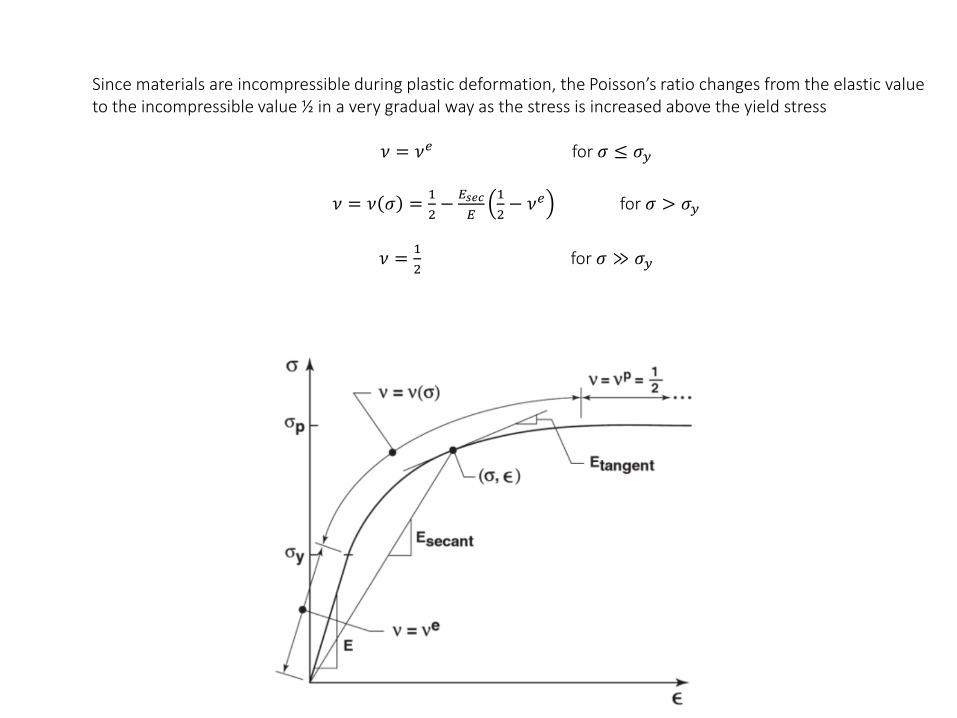
Since materials are incompressible during plastic deformation, the Poisson’s ratio changes from the elastic value to the incompressible value ½ in a very gradual way as the stress is increased above the yield stress
𝜈 = 𝜈𝑒 for 𝜎 ≤ 𝜎𝑦
𝜈 = 𝜈 𝜎 =1
2−
𝐸𝑠𝑒𝑐
𝐸
1
2− 𝜈𝑒 for 𝜎 > 𝜎𝑦
𝜈 =1
2for 𝜎 ≫ 𝜎𝑦

Stress-strain relations according to the deformation theory
Strains are separated by Hencky et al. into elastic and plastic strains:
𝜀𝑥 = 𝜀𝑥𝑒 + 𝜀𝑥
𝑝
𝛾𝑥𝑦 = 𝛾𝑥𝑦𝑒 + 𝛾𝑥𝑦
𝑝
The elastic strains are obtained from the Hooke’s law
𝜀𝑥𝑒 =
1
𝐸𝜎𝑥 − 𝜈𝑒 𝜎𝑦 + 𝜎𝑧
𝜀𝑦𝑒 =
1
𝐸𝜎𝑦 − 𝜈𝑒 𝜎𝑥 + 𝜎𝑧
𝜀𝑧𝑒 =
1
𝐸𝜎𝑧 − 𝜈𝑒 𝜎𝑥 + 𝜎𝑦
𝛾𝑥𝑦𝑒 =
𝜏𝑥𝑦𝐺
𝛾𝑦𝑧𝑒 =
𝜏𝑦𝑧𝐺
𝛾𝑧𝑥𝑒 =
𝜏𝑧𝑥𝐺
Where the mechanical properties E and G are the normal elastic modulus and shear modulus

To obtain the plastic moduli we need to consider the stress-strain diagram in terms of the normal stress and the plastic strain
The plastic modulus at any stress above the yield stress is the secant modulus at that pointSo
𝜀𝑥𝑝 =
1
𝐸𝑝𝜎𝑥 − 𝜈𝑝 𝜎𝑦 + 𝜎𝑧
𝜀𝑦𝑝 =
1
𝐸𝑝𝜎𝑦 − 𝜈𝑝 𝜎𝑥 + 𝜎𝑧
𝜀𝑧𝑝 =
1
𝐸𝑝𝜎𝑧 − 𝜈𝑝 𝜎𝑥 + 𝜎𝑦
𝛾𝑥𝑦𝑝 =
𝜏𝑥𝑦𝐺𝑝
𝛾𝑦𝑧𝑝 =
𝜏𝑦𝑧𝐺𝑝
𝛾𝑧𝑥𝑝 =
𝜏𝑧𝑥𝐺𝑝
Where 𝜈𝑝 is the plastic Poisson’s ratio (1/2) and 𝐺𝑝 is the plastic shear modulus:
𝐺𝑝 =𝐸𝑝
2 1 + 𝜈=𝐸𝑝
3

The elastic and plastic strains sum to the total strains
1
𝐸𝑠𝑒𝑐=1
𝐸+
1
𝐸𝑝
𝜈 = 𝜈𝑒 𝐸 + 𝜈𝑝 𝐸𝑝
1 𝐸 + 1 𝐸𝑝
The stress-strain behavior is divided into three regions: elastic, elastic-plastic and plastic
Only the elastic-plastic region is considered in the deformation theory as a material nonlinearity because plastic poisson’s ratio is constant

Partitioning of the strains into elastic and plastic components is used in derivation of the deformation theory. Deformation theory enables us determine the strains from a state of multiaxial stress, in a single form that applies to all three deformation regions
These total stress-strain relations for an isotropic material in terms of the secant modulus and a continuously variable Poisson’s ratio are similarly:
𝜎𝑥 =𝐸𝑠𝑒𝑐𝑎𝑛𝑡
1 + 𝜈 1 − 2𝜈1 − 𝜈 𝜀𝑥 + 𝜈 𝜀𝑦 + 𝜀𝑧
𝜎𝑦 =𝐸𝑠𝑒𝑐𝑎𝑛𝑡
1 + 𝜈 1 − 2𝜈1 − 𝜈 𝜀𝑦 + 𝜈 𝜀𝑧 + 𝜀𝑥
𝜎𝑥 =𝐸𝑠𝑒𝑐𝑎𝑛𝑡
1 + 𝜈 1 − 2𝜈1 − 𝜈 𝜀𝑧 + 𝜈 𝜀𝑥 + 𝜀𝑦
𝜏𝑦𝑧 =𝐸𝑠𝑒𝑐𝑎𝑛𝑡2 1 + 𝜈
𝛾𝑦𝑧 = 𝐺𝑠𝑒𝑐𝑎𝑛𝑡𝛾𝑦𝑧
𝜏𝑧𝑥 =𝐸𝑠𝑒𝑐𝑎𝑛𝑡2 1 + 𝜈
𝛾𝑧𝑥 = 𝐺𝑠𝑒𝑐𝑎𝑛𝑡𝛾𝑧𝑥
𝜏𝑥𝑦 =𝐸𝑠𝑒𝑐𝑎𝑛𝑡2 1 + 𝜈
𝛾𝑥𝑦 = 𝐺𝑠𝑒𝑐𝑎𝑛𝑡𝛾𝑥𝑦
Where
𝜈 =1
2−𝐸𝑠𝑒𝑐𝐸
1
2− 𝜈𝑒
And
𝐺𝑠𝑒𝑐𝑎𝑛𝑡 =𝐸𝑠𝑒𝑐
2 1 + 𝜈
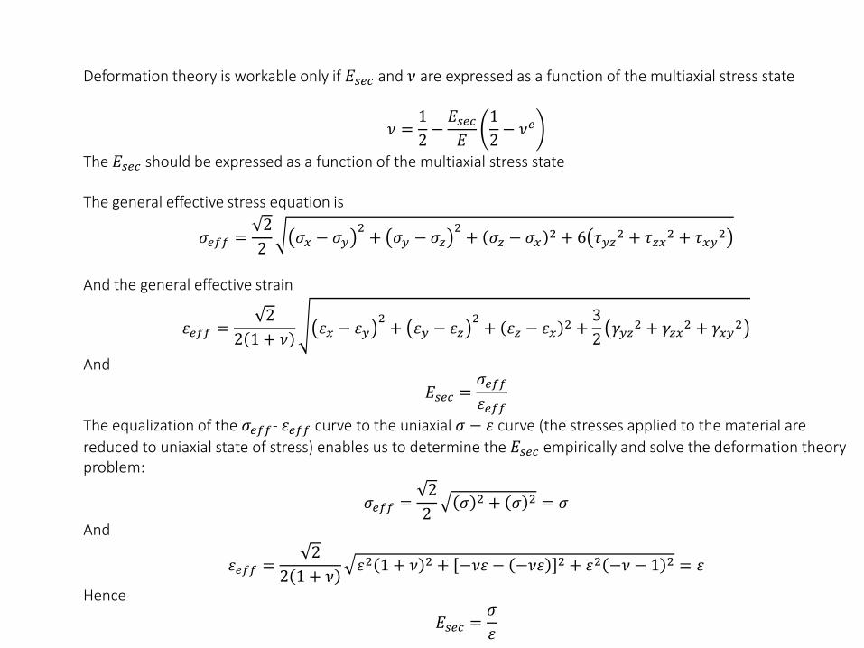
Deformation theory is workable only if 𝐸𝑠𝑒𝑐 and 𝜈 are expressed as a function of the multiaxial stress state
𝜈 =1
2−𝐸𝑠𝑒𝑐𝐸
1
2− 𝜈𝑒
The 𝐸𝑠𝑒𝑐 should be expressed as a function of the multiaxial stress state
The general effective stress equation is
𝜎𝑒𝑓𝑓 =2
2𝜎𝑥 − 𝜎𝑦
2+ 𝜎𝑦 − 𝜎𝑧
2+ 𝜎𝑧 − 𝜎𝑥
2 + 6 𝜏𝑦𝑧2 + 𝜏𝑧𝑥
2 + 𝜏𝑥𝑦2
And the general effective strain
𝜀𝑒𝑓𝑓 =2
2 1 + 𝜈𝜀𝑥 − 𝜀𝑦
2+ 𝜀𝑦 − 𝜀𝑧
2+ 𝜀𝑧 − 𝜀𝑥
2 +3
2𝛾𝑦𝑧
2 + 𝛾𝑧𝑥2 + 𝛾𝑥𝑦
2
And
𝐸𝑠𝑒𝑐 =𝜎𝑒𝑓𝑓𝜀𝑒𝑓𝑓
The equalization of the 𝜎𝑒𝑓𝑓- 𝜀𝑒𝑓𝑓 curve to the uniaxial 𝜎 − 𝜀 curve (the stresses applied to the material are
reduced to uniaxial state of stress) enables us to determine the 𝐸𝑠𝑒𝑐 empirically and solve the deformation theory problem:
𝜎𝑒𝑓𝑓 =2
2𝜎 2 + 𝜎 2 = 𝜎
And
𝜀𝑒𝑓𝑓 =2
2 1 + 𝜈𝜀2 1 + 𝜈 2 + −𝜈𝜀 − −𝜈𝜀 2 + 𝜀2 −𝜈 − 1 2 = 𝜀
Hence
𝐸𝑠𝑒𝑐 =𝜎
𝜀

Relating the material properties 𝐸𝑠𝑒𝑐, 𝜈 for deformation under a multiaxial stress state to the properties determined in the usual uniaxial mechanical characterization test is important especially for materials with nonlinear stress-strain behavior as their properties are a nonlinear function of all the multiaxial stresses that act.
The 𝜎 − 𝜀 curve obtained from the uniaxial test is the same as the 𝜎𝑒𝑓𝑓- 𝜀𝑒𝑓𝑓 curve which represents all multiaxial
stresses. This remarkable identity makes the uniaxial stress-strain curve the universal stress-strain curve

Procedure to obtain the secant modulus form a uniaxial stress-strain curve:Basically the curve should be considered as a set of points each of which is a stress and corresponding strain that are obtained during a measurement.
• Mark the stress-strain curve at a specific value of 𝜎𝑒𝑓𝑓 corresponding to the given multiaxial stress state
• Determine 𝐸𝑠𝑒𝑐 graphically by drawing a straight line to the origin.• Use 𝐸𝑠𝑒𝑐 and the variable 𝜈 in the stress-strain relations to calculate the strains for the specified 𝜎𝑒𝑓𝑓• The strains 𝜀𝑥, 𝜀𝑦, 𝜀𝑧, 𝛾𝑥𝑦 , 𝛾𝑦𝑧, 𝛾𝑧𝑥 that are given below are the answers we are looking for, not 𝜀𝑒𝑓𝑓 that can
be obtained directly from the curve.
𝜀𝑥 =1
𝐸𝑠𝑒𝑐𝜎𝑥 − 𝜈 𝜎𝑦 + 𝜎𝑧
𝜀𝑦 =1
𝐸𝑠𝑒𝑐𝜎𝑦 − 𝜈 𝜎𝑥 + 𝜎𝑧
𝜀𝑧 =1
𝐸𝑠𝑒𝑐𝜎𝑧 − 𝜈 𝜎𝑥 + 𝜎𝑦
𝛾𝑥𝑦 =𝜏𝑥𝑦𝐺𝑝
𝛾𝑦𝑧 =𝜏𝑦𝑧𝐺𝑝
𝛾𝑧𝑥 =𝜏𝑧𝑥𝐺𝑝

Example – Use the stress-strain diagram for Nickel (𝜈 = 0.31) to calculate its elastic modulus and secant modulus for an effective stress state of 400 MPa.

Example – Use the stress-strain diagram for Zinc (𝜈 = 0.29) to calculate its elastic modulus, secant modulus and resulting strains for a plane stress state of
𝜎𝑥 = 70 𝑀𝑃𝑎, 𝜎𝑥 = 50 𝑀𝑃𝑎, 𝜏𝑥𝑦 = 60 𝑀𝑃𝑎

The modulus is expressed as a function of the stresses using various material models.
Although the secant modulus is dynamic and depends on the stress level, the problem-solving becomes straight-forward with the help of stress-strain diagrams or models that include strain hardening
Hencky used the von Mises yield criterion and the distortional energy concept to derive the stress-strain relations
The combination of the yield criterion, the stress-strain relations, and the material model gives the complete deformation theory of plasticity
Deformation theory helps us predict the stresses and strains at a point on the stress-strain curve but does not consider the path taken to get there.
Because of that, loading and unloading can not be evaluated with the same material model using deformation theory and should be considered as separate events.
Another limitation of deformation theory is that all stresses in a multiaxial stress state must be applied in proportion to one another because deformation theory is not capable of distinguishing between types of loading.
These restrictions are valid for some plasticity problems and the theory is not generally applicable.
But it is applicable to most practical problems in metal forming and quite useful. Some problems that are easily solved with deformation theory are difficult to solve with incremental theory because of the excessively complex computation methods.

Proportional loading is when a material is loaded in such a way that the components of the deviatoric stress maintain proportionality throughout the load history
It is represented by a straight line passing through the origin in the principal stress space:
The components of deviatoric stresses for a proportional loading are represented as
𝜎𝑖𝑗 = 𝐾 ∗ 𝜎𝑖𝑗0
Where K is a monotonically increasing function (loading only) and 𝜎𝑖𝑗0 is an arbitrary state of stress


Hydrostatic and Deviatoric Stresses
Total stress tensor can be divided into two components:1. Hydrostatic or mean stress tensor (𝜎𝑚) involving only pure tension or compression
2. Deviatoric stress tensor (𝜎𝑖𝑗′ ) representing pure shear with no normal components

On the other hand, increments of strain are related to increments of stress as loading progresses in the incremental strain theory.The stress history is accounted for by summing the stress increments (by integrating over the loading path to the final stress state)The strains and stresses are related with a complicated nonlinear function that depends on the loading path
Stress history is important in deformation analysis because the final strain states for two identical final stress states may be different if they have different stress histories.
Consider a thin tube subjected to combinations of torsion and axial tension:
The loading in two dimensional stress space is represented for an isotropically hardening tube material as
Under simple uniaxial tension along the lone OAB, the material first yields at point A and then strain hardens to point B. The permanent plastic normal strains and the resulting elastic strains at point B are

The second simple load path is pure shear along line OCD. Again the material yields at point C and strain hardens to point D. The permanent plastic strain and the resultant elastic strain at point D is
The permanent plastic strains remaining in the tube are quitedifferent for the two cases:
However their effective stresses are equal (since they are on the same yield curve)
Thus they have yielded quite differently due to the different stress histories
minus
minus
E

The load paths considered are combinations of nonproportional stress components
Thus nonproportional loading leads to stress history dependence of the final strain state for a body.
The plastic deformation at point E can be calculated using deformation theory if the path OE is considered
In that case the plastic strains would be a mixture of normal and shear strains, which is very different from the unproportional paths both quantitatively and qualitatively.
Accordingly, we must recognize the dependence of our solution approach on the type of load path in a specific plasticity problem.
In reality the plastic strain is a function of both stresses and stress history.So following the deformation in a step by step manner during loading process by the incremental theory gives the most accurate analysis of deformation.
Where K=1/Etan
Integrate the equation for a prescribed load path