plasma sheet turbulence observed by cluster ii

Plasma sheet turbulence observed by Cluster II

James M. Weygand,1 M. G. Kivelson,1 K. K. Khurana,1 H. K. Schwarzl,1

S. M. Thompson,1 R. L. McPherron,1 A. Balogh,2 L. M. Kistler,3 M. L. Goldstein,4

J. Borovsky,5 and D. A. Roberts4

Received 10 May 2004; revised 15 September 2004; accepted 2 November 2004; published 14 January 2005.

[1] Cluster fluxgate magnetometer (FGM) and ion spectrometer (CIS) data are employedto analyze magnetic field fluctuations within the plasma sheet during passages through themagnetotail region in the summers of 2001 and 2002 and, in particular, to look forcharacteristics of magnetohydrodynamic (MHD) turbulence. Power spectral indicesdetermined from power spectral density functions are on average larger thanKolmogorov’s theoretical value for fluid turbulence as well as Kraichnan’s theoreticalvalue for MHD plasma turbulence. Probability distribution functions of the magneticfluctuations show a scaling law over a large range of temporal scales with non-Gaussiandistributions at small dissipative scales and inertial scales and more Gaussian distributionat large driving scales. Furthermore, a multifractal analysis of the magnetic fieldcomponents shows scaling behavior in the inertial range of the fluctuations from about20 s to 13 min for moments through the fifth order. Both the scaling behavior of theprobability distribution functions and the multifractal structure function suggest thatintermittent turbulence is present within the plasma sheet. The unique multispacecraftaspect and fortuitous spacecraft spacing allow us to examine the turbulent eddy scale sizes.Dynamic autocorrelation and cross correlation analysis of the magnetic field componentsallow us to determine that eddy scale sizes fit within the plasma sheet. These resultssuggest that magnetic field turbulence is occurring within the plasma sheet resulting inturbulent energy dissipation.

Citation: Weygand, J. M., et al. (2005), Plasma sheet turbulence observed by Cluster II, J. Geophys. Res., 110, A01205,

doi:10.1029/2004JA010581.

1. Introduction

1.1. Turbulence

[2] There is no standard agreed upon definition ofturbulence. However, we tend to think of turbulence asthe break-up of fluid/plasma flow into whorls and eddies thatcontinue to break down into smaller eddies. Kolmogorov[1941] first described the break up of whorls and eddies asthe cascade of energy from driving scales (convectionscales) where energy is put into the system, through inertialscales (eddy break-down scales), to dissipative scales whereviscosity takes over (heating on the scale of individualparticles). In this study we will define turbulence as randomoscillations of flow or magnetic fields set up by instabilities[Kadomtsev, 1965], and as an eddy-like state of fluidmotion where the inertial vortex forces in eddies are larger

than the forces that tend to damp eddies out [Leung andGibson, 2005].

1.2. Turbulence in the Plasma Sheet

[3] Critical to enhancing our understanding of magneto-spheric dynamics is improved knowledge of how electro-magnetic energy stored in the magnetotail is transferred toplasma energy. Theorists including Borovsky et al. [1997],Borovsky and Funsten [2003], Chang [1999], and Klimas etal. [2000] have proposed a central role for turbulent flows inplasma sheet dynamics, but measurements to characterizespatial and temporal variations independently have not beenavailable to confirm the existence of plasma sheet turbulenceand establish its role in energy transport. Initially,Borovsky etal. [1997] applied techniques useful in solar wind analysis tothe magnetosphere’s plasma sheet and suggested that MHDturbulence is present in the plasma sheet. They quantified theturbulent eddy scale size as �4,000 km to 10,000 km[Borovsky et al., 1997; Neagu et al., 2001] and postulatedthat velocity shear instabilities drive the turbulent fluctua-tions. Thatwork employs data from a single spacecraft, whichcannot distinguish between spatial and temporal changes.

1.3. Identifying Turbulence

[4] The solar wind is turbulent and solar wind turbulencehas been identified in various ways. The methods of identi-

JOURNAL OF GEOPHYSICAL RESEARCH, VOL. 110, A01205, doi:10.1029/2004JA010581, 2005

1Institute of Geophysics and Planetary Physics, University ofCalifornia, Los Angeles, California, USA.

2Imperial College of Science and Technology, London, UK.3Institute for the Study of Earth, Oceans, and Space, University of New

Hampshire, Durham, New Hampshire, USA.4Goddard Space Flight Center, Greenbelt, Maryland, USA.5Los Alamos National Laboratory, Los Alamos, New Mexico, USA.

Copyright 2005 by the American Geophysical Union.0148-0227/05/2004JA010581$09.00

A01205 1 of 24

fication include: Reynolds numbers [Goldstein et al., 1997],power spectral density spectra in the frequency domain[Coleman, 1968; Goldstein and Roberts, 1999], ruggedinvariants [Matthaeus and Goldstein, 1982; Goldstein etal., 1995], probability density functions of both magneticand velocity fluctuations [Sorriso-Valvo et al., 1999], andmagnetic field and velocity multifractal analysis [Burlagaand Klein, 1986; Burlaga, 1991a, 1991b, 1991c]. Some ofthese techniques can be applied to the plasma sheet.[5] Initial work to identify turbulence within the space

plasmas focused on the spectral index within the inertialrange of the power spectral density fall off in thefrequency domain [Coleman, 1968]. The inertial rangewithin power spectra consists of the region bounded byfrequencies related to the large-scale driving of theplasma flow, equivalent to the inverse of the convectiveperiod in the plasma sheet, and frequencies relevant tothe small-scale heating of the plasma, which can beequated with the gyrofrequency of the ions. Turbulence,however, refers to spatial fluctuations generated in amedium by instability. If the Taylor hypothesis applies,there is a close relation between the temporal and spatialfluctuations. The Taylor hypothesis states that frequencyw is linearly related to the wave vector k (i.e., w = k � v,where v is the plasma velocity) and is applicable if thestructures within the magnetic field and flow evolve on atimescale longer than the time it takes them to pass thespacecraft.[6] Kolmogorov [1941] and Kraichnan [1965] assume the

validity of the Taylor Hypothesis and predict values of thespectral index in a turbulent medium. Kolmogorov [1941],who examined neutral fluid turbulence, derived a spectralindex of �5/3. Kraichnan [1965] calculated a value of�3/2 for ideal isotropic incompressible MHD turbulencein a conducting fluid. The difference between the twovalues is related to the number of degrees of freedom inthe fluid flow. In both derivations, the rate of energytransfer from the driving scale of the spectra to the heatingrange of the spectra is assumed to be constant. This factwill be important for differentiating Kolmogorov andKraichnan type turbulence from intermittent turbulence.[7] Within the plasma sheet Borovsky et al. [1997]

found that the slope of the power spectral density versusfrequency for plasma flow velocity and magnetic fieldvaried from �0.8 to �2.0 and �1.6 to �3.0, respectively.Although the ranges of these values include one or bothof the theoretical predictions, they do not confirm thatturbulence is present within the plasma sheet. The widerange of values could be explained by several differentphenomena in the plasma sheet. Borovsky and Funsten[2003] suggest that the range of spectral indices couldresult from boundary effects or a combination of drivingmechanisms each exhibiting different spectral indices. Therange of spectral indices could also result from intermit-tent turbulence, a mechanism that we will discuss furtherin this study. The fact that various phenomena in theplasma sheet affect spectral indices implies that this toolis not useful for identifying the presence of intermittentturbulence. The situation is different in the solar windwhere boundary effects are not a problem and thefluctuations are stationary [Matthaeus and Goldstein,1982].

[8] The fact that a spectral index of �2 can arise fromintermittent turbulence leads us to investigate further thepossibility that plasma sheet fluctuations satisfy conditionsfor intermittency. Intermittent turbulence is defined asturbulence with a fluctuating rate of energy transfer fromthe driving scale of the spectra to the heating range of thespectrum. Non-self-similar scaling of probability distribu-tion functions (PDFs) of the fluctuations in the flow ormagnetic field can be used to identify intermittent turbu-lence. Fluctuations of the difference of magnetic fieldcomponents observed at two locations with large spatialseparation will have nearly Gaussian PDFs with a fourthmoment, referred to as the kurtosis, of approximately 3.This means that the values at the two locations are unrelated.If intermittent turbulence is present within the flow ormagnetic field, then differences between values at smallerspatial separations will have larger kurtoses than for largeseparations and the kurtosis will systematically decreasewith increasingly large separation. A distribution with akurtosis larger than 3 has a greater probability of largefluctuations in the wings of the distribution than in thewings of a Gaussian distribution. The high probability oflarge fluctuations in the wings is due to excess energy at thedriving scales generating the larger fluctuations. The com-parison of the PDFs at a range of spatial separations hasbeen developed for and successfully used to analyze labo-ratory plasma experiments [Castaing et al., 1990; Naert etal., 1994].[9] Sorriso-Valvo et al. [1999, 2001] examined intermit-

tency in MHD flows and magnetic fields by using space-craft measurements of the solar wind. They demonstratedthat PDFs of the flow and magnetic field fluctuations havebroader wings, than Gaussian distributions over smallspatial scales. The PDFs become more Gaussian for spatialseparations much larger than turbulent eddy scales. Basedon these facts Sorriso-Valvo et al. concluded that the solarwind is intermittently turbulent. As far as the authors areaware, no one has examined the scaling of the PDF of theflow or the magnetic field fluctuations within the magneto-sphere’s plasma sheet.[10] Hnat et al. [2002] also showed intermittency is

present in the solar wind magnetic field fluctuations. Theydemonstrated that these PDFs exhibit approximate mono-power scaling law in the inertial range of 46 s to 26 hoursusing the functional form:

P dB2; t� �

¼ t�sPs dB2t�s; t� �

; ð1Þ

where dB2 = B2(t + t) � B2(t), t is the scale size (i.e., thetemporal separation over which the magnetic field fluctua-tion is identified), and s is the constant scaling exponent.Chang et al. [2004] has applied the Hnat et al. [2002]technique to their model of intermittent turbulence fluctua-tions arising from coexisting nonpropagating spatiotemporalfluctuations and propagating modes in a space plasma.Their results showed the same non-Gaussian shape at smallscales and Gaussian shape at larger scales for the unscaledPDFs as observed by Sorriso-Valvo et al. [1999, 2001] andHnat et al. [2002]. When Chang et al. [2004] rescale thePDFs they find that PDFs in regions far from the neutralsheet do exhibit a monoscaling law, but PDFs near theneutral sheet do not rescale exactly.

A01205 WEYGAND ET AL.: PLASMA SHEET TURBULENCE

2 of 24

A01205

[11] Whereas the kurtosis can show that the PDFs offluctuations become less Gaussian as the spatial separationof the measurement positions decreases, there is no reasonto limit the analysis to the fourth moment of the distribu-tions. Evaluation of the multifractal structure of the fluctua-tions provides a more robust method for demonstratinganomalous scaling of flow and magnetic field. In fullydeveloped solar wind turbulent regions, Burlaga [1991a]has shown:

Bi tnð Þ=hBi tnð Þið Þpj jh i / ts pð Þn ; ð2Þ

where Bi (tn) is the time series composed of data averagedover intervals of duration tn = 2n Dt (n = 0, 1, 2,. . ..) with Dtthe resolution of the time series data and p an integer. Thepointed brackets represent averages over the entire intervalbeing analyzed. The procedure is equivalent to obtaining thepth moment of the averaged time series. In a turbulentmedium with a constant rate of energy transfer from thedriving scales to the dissipation scales, the scaling exponentfunction, s(p), is linear (i.e., Kolmogorov and Kraichnantype turbulence) and the medium is considered to have selfsimilar scaling properties. If the fluctuations are intermit-tently turbulent (i.e., the rate of energy transfer fluctuates),then s(p) will be nonlinear and the medium is considered toshow anomalous scaling properties [L’vov and Procaccia,1998]. Solar wind studies of the flow velocity and themagnetic field have found anomalous scaling. For the flows(p) is a quadratic function [Burlaga, 1991b, 1991c] and forthe magnetic field it is a cubic function [Burlaga, 1992].Recent work by Lui [2001, 2002] and Voros et al. [2003]has found anomalous scaling properties in the plasma sheetat kinetic scales. Lui [2001] examined the multifractalnature of substorm-associated magnetic turbulence in themagnetotail using a method similar to that indicated withequation (2). He reported scaling exponents with nonlineardependence for orders of moments from �5 to 5 (similar tothe Burlaga studies in the solar wind) associated withmagnetic field line fluctuations and he showed that thenonlinearity depends on the distance from the neutral sheet.Lui [2001] quantifies the degree of intermittency observedby calculating the intermittency coefficient and determinesvalues from 0.18 to 0.42. The intermittency coefficient is ameasure of the nonlinearity in the scaling exponentialfunction [Antonia et al., 1982; Consolini et al., 1996].Within the solar wind flow data Burlaga [1991a, 1993]determined intermittency coefficient values of 0.19 ± 0.02and 0.28 ± 0.27.[12] Voros et al. [2003] demonstrated that the magnetic

field fluctuations in the plasma sheet have multiscalefeatures using an algorithm that quantified intermittenceon the basis of statistical distributions.[13] All previous studies of space plasma turbulence used

data from a single spacecraft. If the Taylor hypothesis isvalid, a single spacecraft can probe the spatial structure ofthe system that can be regarded as effectively unchangingduring a transport interval. Plasma sheet studies haveimplicitly assumed the Taylor hypothesis, even though itis not normally applicable because the flow speeds rarelyexceed the Alfven speed. The advent of Cluster II, a fourspacecraft mission, provides a new tool that allows us tomeasure the magnetic field simultaneously at spatially

separated locations. In this study we take advantage of thehigh time resolution and multispacecraft capability of Clus-ter II to further investigate the turbulence in the plasmasheet, applying the techniques discussed above to showquantitatively that intermittent turbulence is present withinthe magnetosphere’s plasma sheet.

2. Instrumentation

[14] The Cluster mission, supported jointly by the Euro-pean Space Agency (ESA) and NASA, consists of fouridentical spinning spacecraft (spin period of 4 s) closelyspaced in orbits with a perigee of 4 RE, an apogee of about19.6 RE. The spacecraft were launched in the summer of2000. In the summers of 2001 and 2002, the apogee of theorbit was in the magnetotail and near apogee the fourspacecraft spanned a nearly regular tetrahedron with inter-spacecraft spacings of approximately 1,000 km in 2001 andabout 5,000 km in 2002. Between late July and earlyNovember in both 2001 and 2002 the orbits provided a fullseason of plasma sheet crossings. Cluster spends from about6 hours to 12 hours within the plasma sheet on each orbit,which makes it ideal for plasma sheet studies. At this timewe have identified some 67 plasma sheet crossings onwhich there were no data gaps.[15] Each Cluster spacecraft carries a boom mounted

triaxial fluxgate magnetometer 5.2 m from the craft [Baloghet al., 1997]. Magnetic field vectors are sampled at a rate of201.75 vectors s�1, and either 22 Hz data (nominal mode)or 67 Hz data (burst mode) are transmitted to Earth. Bothpreflight and in-flight calibration of the two magnetometershas been performed to produce carefully calibrated (andintercalibrated) data that minimize errors in the magneticfield measurements.[16] There are two plasma detectors, the Cluster ion

spectrometers (CISs), on each spacecraft [Reme et al.,1997]. They are the hot ion analyzer, which is anasymmetric quadrispherical electrostatic analyzer, andthe time-of-flight composition and distribution functiondetector. CIS records a three-dimensional ion distributionwith a mass resolution (M/DM) of 4 between 1 amu and32 amu. This instrument will play a key role in identi-fying periods when Cluster enters the plasma sheet,which is characterized by high electron and ion temper-atures as well as significant H+, He+, and O+ populations.CIS will be used here to provide fundamental plasmaparameters such as density, velocity vectors, pressuretensor, and heat flux.[17] Absolute errors in most of the measure values are not

critical for this study except for the uncertainty associatedwith the flow. The flow components in the spin plane(normal to the ecliptic) are better determined than thecomponent along the spin axis. Along the spin axis themean flow is assumed to be zero, but there are systematicerrors from slight errors in the calibration. The uncertaintyin the component along the spin axis based on thesesystematic errors is about ±15 km s�1.

3. Observations

[18] Observations from magnetotail seasons show thatwhen the spacecraft are in the current sheet, the magnetic


3 of 24

A01205

field, flow, and current density fluctuate rapidly over time-scales of seconds to tens of minutes. Data from the Clustermultispacecraft mission provide the first opportunity toexamine both spatial and temporal variations associatedwith turbulence and thereby to develop insight into thestructure of fields and flows. This work will examineplasma sheet fluctuations on four passes, three from the2001 season and one from the 2002 season. We analyze thefluctuations using two techniques that have previously beenapplied to the solar wind and find evidence for turbulence inall four events. The first approach is the scaling of theprobability distribution functions of magnetic field fluctua-tions, a technique used by Sorriso-Valvo et al. [1999], andthe second approach is a multifractal method used byBurlaga [1991a, 1991b, 1991c].

3.1. August 15, 2001

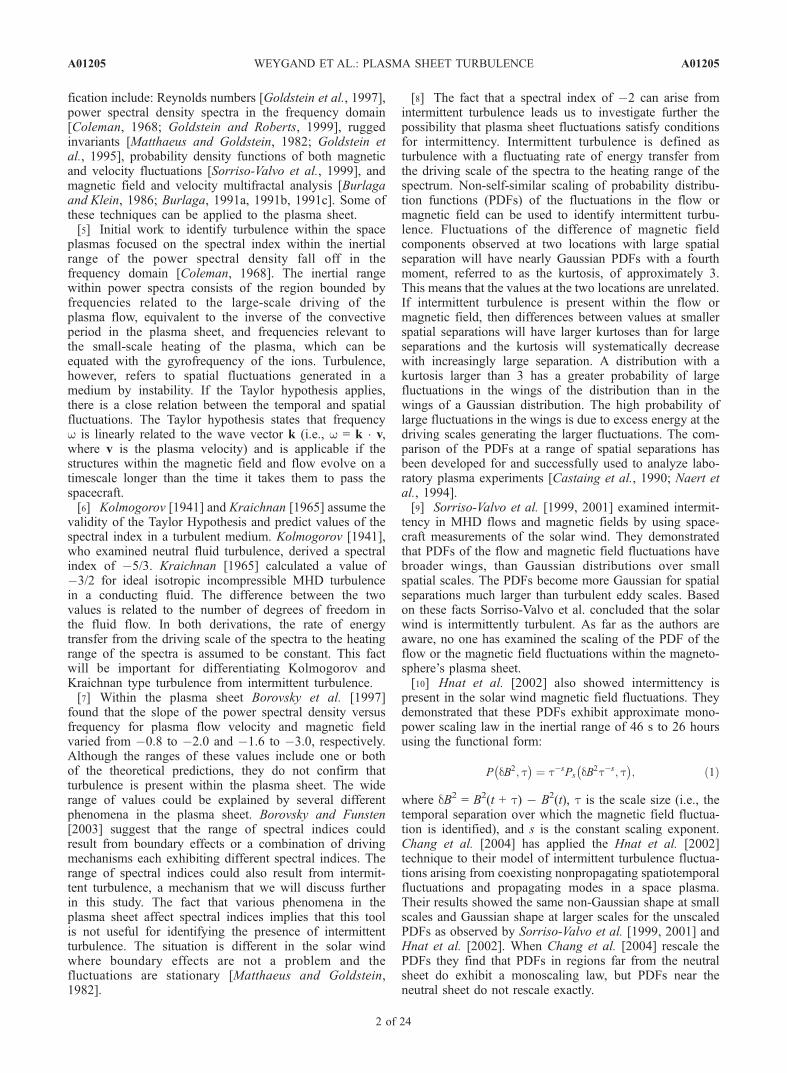
[19] Figure 1 displays the magnetic field data fromCluster spacecraft 1 for the plasma sheet crossing onAugust 15, 2001. The plasma sheet crossing lasts from0130 UT to 1330 UT. The interspacecraft spacing duringthis event is approximately 1,000 km at apogee. In firstpanel it is evident that the crossing from the northern lobeto the southern lobe occurred at about 0900 UT when Bx

reversed sign. The lower three panels (B1, B2, and B3) arethe components of the magnetic field in a field-alignedcoordinate system determined at the midpoint of an 80-minaverage. The B1 component is along the average magneticfield. The B2 component is the magnetic field in thedirection perpendicular to B1 and to the radial directionfrom Earth (approximately the azimuthal direction in theequatorial plane) and the B3 is the third component ofthe right hand coordinate system (approximately radial inthe equatorial plane). In this system the compressional andtransverse fluctuations in the magnetic field are readilyidentified. The time series data have been divided into fivedifferent regions: the northern lobe (NLobe), northernplasma sheet (NPS), central plasma sheet (CPS), southernplasma sheet (SPS), and the southern lobe (SLobe). Thestart and end of the plasma sheet crossing have beenidentified with both the magnetometer data and the CIS[Reme et al., 1997] density and ion temperature data.[20] The plasma sheet is defined as the region in the

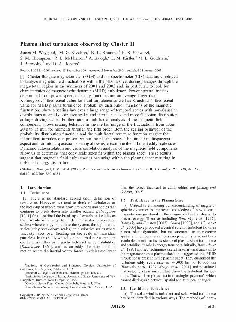
magnetotail where the plasma density and temperaturesignificantly increase above the lobe values and is the regionwhere the Bx component reverses from earthward to anti-earthward. The CPS is arbitrarily defined as the region whereBx GSM is between �10 nT and 10 nT. The strongestfluctuations generally occur for this crossing within theCPS from 0754 UT to 1013 UT. Figure 2 displays a 1-hourperiod during the August 15 plasma sheet crossing andshows in detail the moderate and strong fluctuationsrecorded by all four spacecraft in the NPS and CPS regions.In contrast, magnetic field fluctuations are small or absentwithin the lobe in Figure 1. Indicated with the dark grayvertical lines in Figure 1 are the times of three substormonsets. The substorms occur at about 0130 UT and0434 UT when Cluster is in the NPS, at 0751 UT whenCluster is just entering the CPS, and at 1534 UTwhen Clusteris deep in the SLobe. These substorms are thoroughlydiscussed in several other studies [McPherron et al., 2002;M. G. Kivelson et al., The response of the near Earth

magnetotail to substorm activity, submitted to Advancesin Space Research, 2002]. AE did not exceed 500 nT andhad an average value of 150 nT during this plasma sheetcrossing and Kp was approximately 2-.

3.2. August 21, 2002

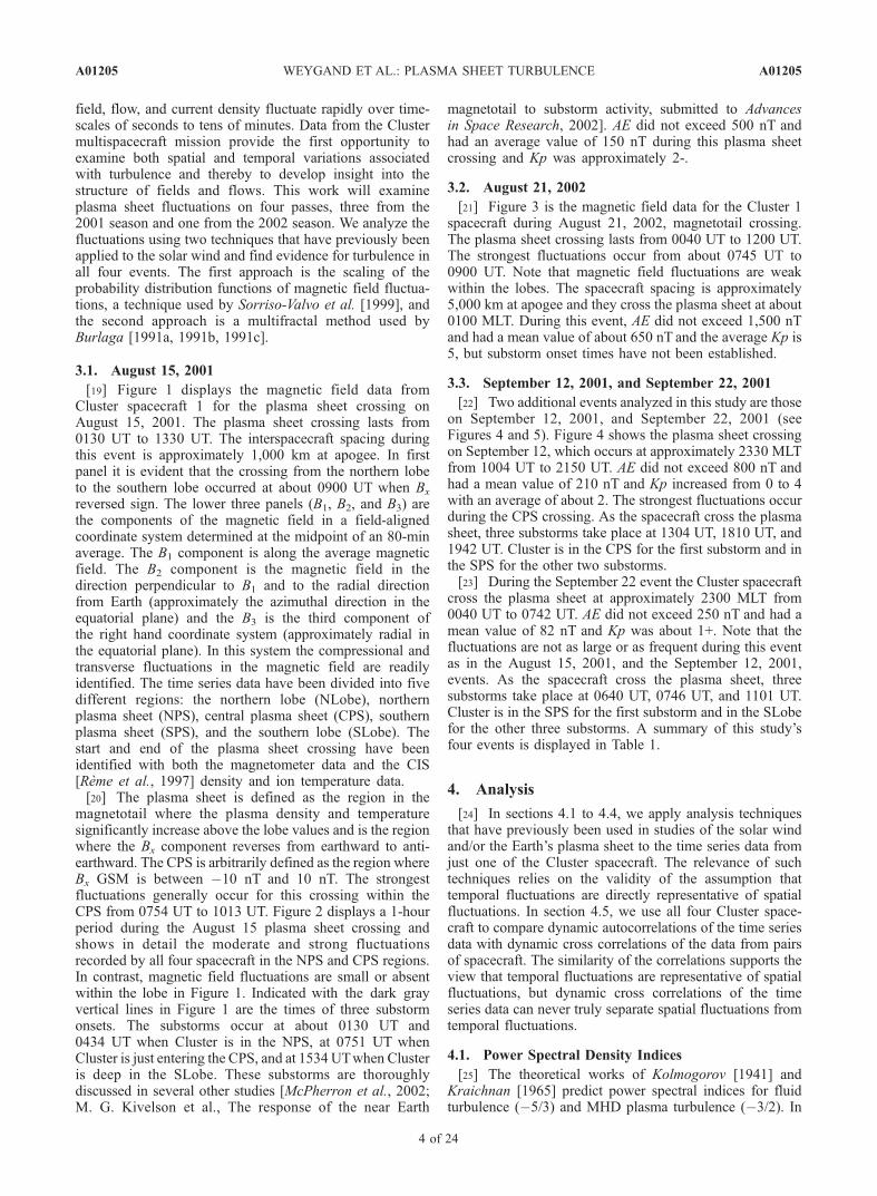
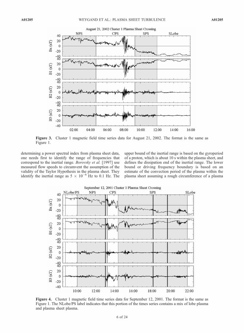
[21] Figure 3 is the magnetic field data for the Cluster 1spacecraft during August 21, 2002, magnetotail crossing.The plasma sheet crossing lasts from 0040 UT to 1200 UT.The strongest fluctuations occur from about 0745 UT to0900 UT. Note that magnetic field fluctuations are weakwithin the lobes. The spacecraft spacing is approximately5,000 km at apogee and they cross the plasma sheet at about0100 MLT. During this event, AE did not exceed 1,500 nTand had a mean value of about 650 nT and the average Kp is5, but substorm onset times have not been established.

3.3. September 12, 2001, and September 22, 2001

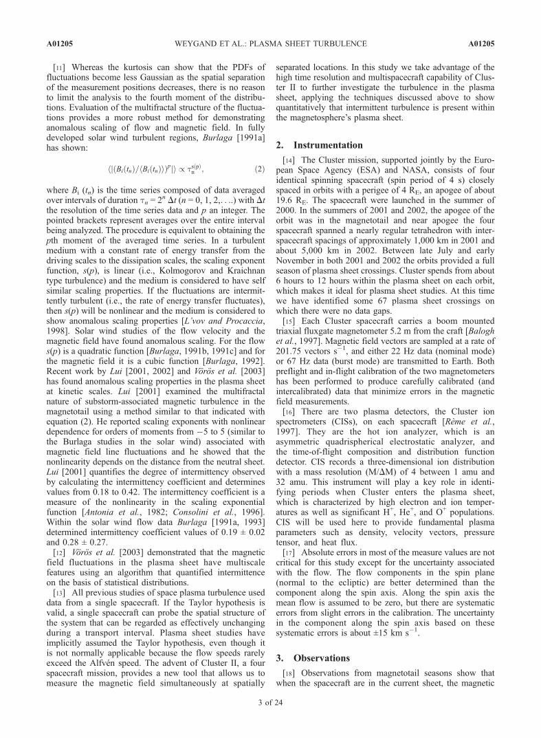
[22] Two additional events analyzed in this study are thoseon September 12, 2001, and September 22, 2001 (seeFigures 4 and 5). Figure 4 shows the plasma sheet crossingon September 12, which occurs at approximately 2330 MLTfrom 1004 UT to 2150 UT. AE did not exceed 800 nT andhad a mean value of 210 nT and Kp increased from 0 to 4with an average of about 2. The strongest fluctuations occurduring the CPS crossing. As the spacecraft cross the plasmasheet, three substorms take place at 1304 UT, 1810 UT, and1942 UT. Cluster is in the CPS for the first substorm and inthe SPS for the other two substorms.[23] During the September 22 event the Cluster spacecraft

cross the plasma sheet at approximately 2300 MLT from0040 UT to 0742 UT. AE did not exceed 250 nT and had amean value of 82 nT and Kp was about 1+. Note that thefluctuations are not as large or as frequent during this eventas in the August 15, 2001, and the September 12, 2001,events. As the spacecraft cross the plasma sheet, threesubstorms take place at 0640 UT, 0746 UT, and 1101 UT.Cluster is in the SPS for the first substorm and in the SLobefor the other three substorms. A summary of this study’sfour events is displayed in Table 1.

4. Analysis

[24] In sections 4.1 to 4.4, we apply analysis techniquesthat have previously been used in studies of the solar windand/or the Earth’s plasma sheet to the time series data fromjust one of the Cluster spacecraft. The relevance of suchtechniques relies on the validity of the assumption thattemporal fluctuations are directly representative of spatialfluctuations. In section 4.5, we use all four Cluster space-craft to compare dynamic autocorrelations of the time seriesdata with dynamic cross correlations of the data from pairsof spacecraft. The similarity of the correlations supports theview that temporal fluctuations are representative of spatialfluctuations, but dynamic cross correlations of the timeseries data can never truly separate spatial fluctuations fromtemporal fluctuations.

4.1. Power Spectral Density Indices

[25] The theoretical works of Kolmogorov [1941] andKraichnan [1965] predict power spectral indices for fluidturbulence (�5/3) and MHD plasma turbulence (�3/2). In


4 of 24

A01205

Figure 2. Magnetic field time series data for August 15, 2001, from 0730 UT to 0830 UT for all fourspacecraft plotted versus universal time. The format is the same as Figure 1. Color is used to distinguishdata from the different Cluster spacecraft: black for Cluster 1, red for Cluster 2, green for Cluster 3, andblue for Cluster 4. See color version of this figure at back of this issue.

Figure 1. Cluster 1 magnetic field time series data in nanoteslas for August 15, 2001, is plotted versusuniversal time. The top panel is the Bx component in GSM coordinates. The lower three panels are themagnetic field components in a field-aligned coordinate system. The plasma sheet crossing has beendivided into five parts that are labeled at the top of the figure: the northern lobe (NLobe), the northernplasma sheet (NPS), the central plasma sheet (CPS), the southern plasma sheet (SPS), and the southernlobe (SLobe). The dark gray vertical lines mark three substorm onsets observed during the plasma sheetcrossing.


5 of 24

A01205

determining a power spectral index from plasma sheet data,one needs first to identify the range of frequencies thatcorrespond to the inertial range. Borovsky et al. [1997] usemeasured flow speeds to circumvent the assumption of thevalidity of the Taylor Hypothesis in the plasma sheet. Theyidentify the inertial range as 5 � 10�6 Hz to 0.1 Hz. The

upper bound of the inertial range is based on the gyroperiodof a proton, which is about 10 s within the plasma sheet, anddefines the dissipation end of the inertial range. The lowerbound or driving frequency boundary is based on anestimate of the convection period of the plasma within theplasma sheet assuming a rough circumference of a plasma

Figure 4. Cluster 1 magnetic field time series data for September 12, 2001. The format is the same asFigure 1. The NLobe/PS label indicates that this portion of the times series contains a mix of lobe plasmaand plasma sheet plasma.

Figure 3. Cluster 1 magnetic field time series data for August 21, 2002. The format is the same asFigure 1.


6 of 24

A01205

sheet convection cell (40 RE) and a mean speed (75 km s�1),which corresponds to a period of about 5 hours. Borovsky etal. [1997] use breakpoints in the power spectra at 1.3 mHzand 42 mHz to further constrain the range of frequenciesfrom which the spectral index is determined.[26] As a first step in this study, we compare properties

of power spectral density in different parts of the plasmasheet with the results of Borovsky et al. [1997]. Thecomparison of results is of interest even though we recog-nize that the spectral indices cannot by themselves demon-strate the presence of turbulence. We assume that the Taylorhypothesis is applicable even though this assumption isalmost certainly not valid within the sub-Alfvenic plasmasheet flows. We use 0.2 s data but we limit comparisonwith the Borovsky et al. results to the frequencies reportedin that study. We find that the average breakpoints in ourpower spectral density plots are about at 2.1 mHz (aboutthe same as Borovsky et al. [1997]) and at 0.1 Hz (nearlymore than double the frequency reported by Borovsky et al.[1997]). We determine the power spectral index separatelyfor each component (B1, B2, and B3) in field-alignedcoordinates and for each plasma sheet region in the fourdifferent cases. The field-aligned coordinate system is usedto differentiate the longitudinal and transverse fluctuations.

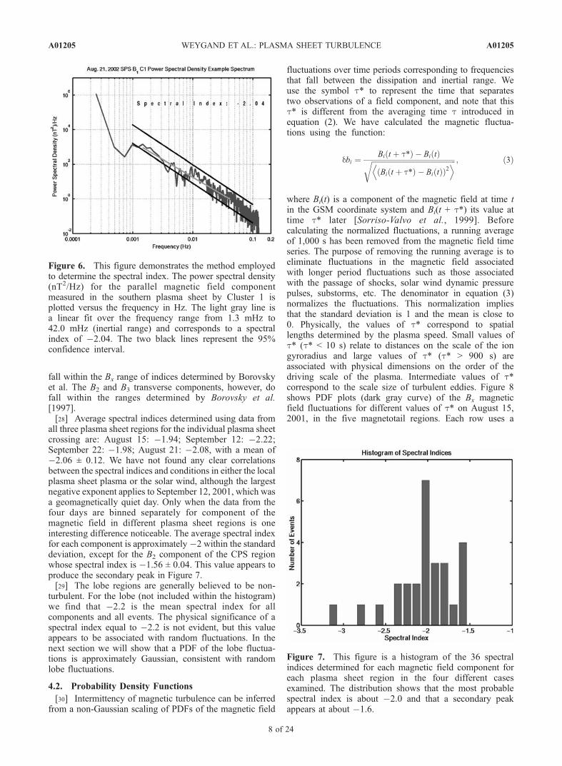
In cases with spectral peaks, we find the slope excludingthe spectral peak of the power spectral density plots.Figure 6 shows an example of the power spectra andour fit to the spectral index within the frequency range ofinterest.[27] From the 36 spectral indices determined (three mag-

netic components times three plasma sheet regions timesfour events examined in this work) a histogram is con-structed (see Figure 7). There is a peak at a spectral index of�2.0 and possibly a secondary peak at about �1.6. Thisdistribution suggests that neither Kolmogorov norKraichnan type turbulence, both of which require constantenergy transfer rates from the driving range to the dissipa-tion range, are present. The most probable index is consis-tent with the presence of intermittent turbulence in theplasma sheet even though this is not the only possibleexplanation [Borovsky and Funsten, 2003]. The range andaverage for each component separately are tabulated andcompared with the Borovsky et al. [1997] results in Table 2.The results in Table 2 show that the findings of this studyare quite similar to those of Borovsky et al. [1997]. Thesevalues, within the uncertainty, are equal, but if we mayroughly equate B1 of our study with Bx from the Borovskyet al. study, the parallel longitudinal component does not

Table 1. Summary of Four Plasma Sheet Crossings Including Date, Time of Apogee, GSM Position of Apogee, Local Time of Apogee,

Kp, and Geomagnetic Activity Based on AE

Event Time of Apogee, UT GSM Position of Apogee (RE) Local Time of Apogee Kp Geomagnetic Activity (AE)

August 15, 2001 0521 (�18.2, �5.7, 2.0) 0109 2� moderateSeptember 12, 2001 1631 (�19.0, 2.8, �0.2) 2330 2 activeSeptember 22, 2001 0414 (�18.4, 5.6, �0.8) 2252 1+ quietAugust 21, 2002 0727 (�18.4, �4.3, 0.5) 0053 5 active

Figure 5. Cluster 1 magnetic field time series data for September 22, 2001. The format is the same asFigure 1. The SLobe/PS label indicates that this portion of the times series contains a mix of lobe plasmaand plasma sheet plasma.


7 of 24

A01205

fall within the Bx range of indices determined by Borovskyet al. The B2 and B3 transverse components, however, dofall within the ranges determined by Borovsky et al.[1997].[28] Average spectral indices determined using data from

all three plasma sheet regions for the individual plasma sheetcrossing are: August 15: �1.94; September 12: �2.22;September 22: �1.98; August 21: �2.08, with a mean of�2.06 ± 0.12. We have not found any clear correlationsbetween the spectral indices and conditions in either the localplasma sheet plasma or the solar wind, although the largestnegative exponent applies to September 12, 2001, which wasa geomagnetically quiet day. Only when the data from thefour days are binned separately for component of themagnetic field in different plasma sheet regions is oneinteresting difference noticeable. The average spectral indexfor each component is approximately �2 within the standarddeviation, except for the B2 component of the CPS regionwhose spectral index is �1.56 ± 0.04. This value appears toproduce the secondary peak in Figure 7.[29] The lobe regions are generally believed to be non-

turbulent. For the lobe (not included within the histogram)we find that �2.2 is the mean spectral index for allcomponents and all events. The physical significance of aspectral index equal to �2.2 is not evident, but this valueappears to be associated with random fluctuations. In thenext section we will show that a PDF of the lobe fluctua-tions is approximately Gaussian, consistent with randomlobe fluctuations.

4.2. Probability Density Functions

[30] Intermittency of magnetic turbulence can be inferredfrom a non-Gaussian scaling of PDFs of the magnetic field

fluctuations over time periods corresponding to frequenciesthat fall between the dissipation and inertial range. Weuse the symbol t* to represent the time that separatestwo observations of a field component, and note that thist* is different from the averaging time t introduced inequation (2). We have calculated the magnetic fluctua-tions using the function:

dbi ¼Bi t þ t*ð Þ � Bi tð ÞffiffiffiffiffiffiffiffiffiffiffiffiffiffiffiffiffiffiffiffiffiffiffiffiffiffiffiffiffiffiffiffiffiffiffiffiffiffiffiffiffiffiffiffiffiffiffiBi t þ t*ð Þ � Bi tð Þð Þ2

D Er ; ð3Þ

where Bi(t) is a component of the magnetic field at time tin the GSM coordinate system and Bi(t + t*) its value attime t* later [Sorriso-Valvo et al., 1999]. Beforecalculating the normalized fluctuations, a running averageof 1,000 s has been removed from the magnetic field timeseries. The purpose of removing the running average is toeliminate fluctuations in the magnetic field associatedwith longer period fluctuations such as those associatedwith the passage of shocks, solar wind dynamic pressurepulses, substorms, etc. The denominator in equation (3)normalizes the fluctuations. This normalization impliesthat the standard deviation is 1 and the mean is close to0. Physically, the values of t* correspond to spatiallengths determined by the plasma speed. Small values oft* (t* < 10 s) relate to distances on the scale of the iongyroradius and large values of t* (t* > 900 s) areassociated with physical dimensions on the order of thedriving scale of the plasma. Intermediate values of t*correspond to the scale size of turbulent eddies. Figure 8shows PDF plots (dark gray curve) of the Bx magneticfield fluctuations for different values of t* on August 15,2001, in the five magnetotail regions. Each row uses a

Figure 6. This figure demonstrates the method employedto determine the spectral index. The power spectral density(nT2/Hz) for the parallel magnetic field componentmeasured in the southern plasma sheet by Cluster 1 isplotted versus the frequency in Hz. The light gray line isa linear fit over the frequency range from 1.3 mHz to42.0 mHz (inertial range) and corresponds to a spectralindex of �2.04. The two black lines represent the 95%confidence interval.

Figure 7. This figure is a histogram of the 36 spectralindices determined for each magnetic field component foreach plasma sheet region in the four different casesexamined. The distribution shows that the most probablespectral index is about �2.0 and that a secondary peakappears at about �1.6.


8 of 24

A01205

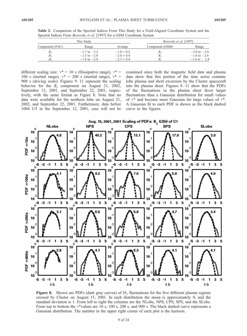
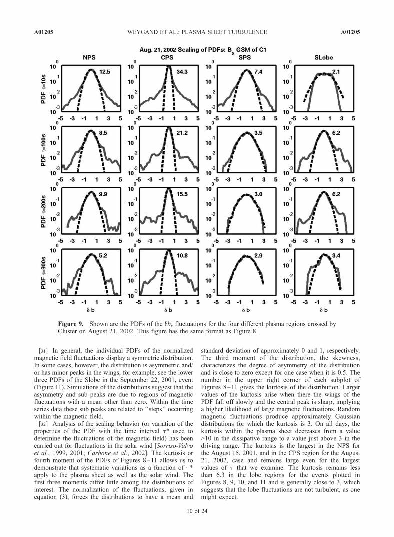
different scaling size: t* = 10 s (Dissipative range), t* =100 s (inertial range), t* = 200 s (inertial range), t* =900 s (driving scale). Figures 9–11 represent the scalingbehavior for the Bx component on August 21, 2002,September 12, 2001, and September 22, 2001, respec-tively, with the same format as Figure 8. Note that nodata were available for the northern lobe on August 21,2002, and September 22, 2001. Furthermore, data before1004 UT in the September 12, 2001, case will not be

examined since both the magnetic field data and plasmadata show that this portion of the time series containslobe plasma and short excursion by the Cluster spacecraftinto the plasma sheet. Figures 8–11 show that the PDFsof the fluctuations in the plasma sheet favor largerfluctuations than a Gaussian distribution for small valuesof t* and become more Gaussian for large values of t*.A Gaussian fit to each PDF is shown as the black dashedcurve in the figures.

Table 2. Comparison of the Spectral Indices From This Study for a Field-Aligned Coordinate System and the

Spectral Indices From Borovsky et al. [1997] for a GSM Coordinate System

This Study Borovsky et al. [1997]

Component (FAC) Range Average Component (GSM) Range

B1 �1.7 to �3.2 �1.8 ± 0.2 Bx �2.0 to �3.0B2 �1.5 to �2.0 �2.0 ± 0.4 By �1.6 to �2.6B3 �1.8 to �2.8 �2.3 ± 0.4 Bz �1.6 to – 2.4

Figure 8. Shown are PDFs (dark gray curves) of dbx fluctuations for the five different plasma regionscrossed by Cluster on August 15, 2001. In each distribution the mean is approximately 0, and thestandard deviation is 1. From left to right the columns are the NLobe, NPS, CPS, SPS, and the SLobe.From top to bottom the t*values are 10 s, 100 s, 200 s, and 900 s. The black dashed curve represents aGaussian distribution. The number in the upper right corner of each plot is the kurtosis.


9 of 24

A01205

[31] In general, the individual PDFs of the normalizedmagnetic field fluctuations display a symmetric distribution.In some cases, however, the distribution is asymmetric and/or has minor peaks in the wings, for example, see the lowerthree PDFs of the Slobe in the September 22, 2001, event(Figure 11). Simulations of the distributions suggest that theasymmetry and sub peaks are due to regions of magneticfluctuations with a mean other than zero. Within the timeseries data these sub peaks are related to ‘‘steps’’ occurringwithin the magnetic field.[32] Analysis of the scaling behavior (or variation of the

properties of the PDF with the time interval t* used todetermine the fluctuations of the magnetic field) has beencarried out for fluctuations in the solar wind [Sorriso-Valvoet al., 1999, 2001; Carbone et al., 2002]. The kurtosis orfourth moment of the PDFs of Figures 8–11 allows us todemonstrate that systematic variations as a function of t*apply to the plasma sheet as well as the solar wind. Thefirst three moments differ little among the distributions ofinterest. The normalization of the fluctuations, given inequation (3), forces the distributions to have a mean and

standard deviation of approximately 0 and 1, respectively.The third moment of the distribution, the skewness,characterizes the degree of asymmetry of the distributionand is close to zero except for one case when it is 0.5. Thenumber in the upper right corner of each subplot ofFigures 8–11 gives the kurtosis of the distribution. Largervalues of the kurtosis arise when there the wings of thePDF fall off slowly and the central peak is sharp, implyinga higher likelihood of large magnetic fluctuations. Randommagnetic fluctuations produce approximately Gaussiandistributions for which the kurtosis is 3. On all days, thekurtosis within the plasma sheet decreases from a value>10 in the dissipative range to a value just above 3 in thedriving range. The kurtosis is the largest in the NPS forthe August 15, 2001, and in the CPS region for the August21, 2002, case and remains large even for the largestvalues of t that we examine. The kurtosis remains lessthan 6.3 in the lobe regions for the events plotted inFigures 8, 9, 10, and 11 and is generally close to 3, whichsuggests that the lobe fluctuations are not turbulent, as onemight expect.

Figure 9. Shown are the PDFs of the dbx fluctuations for the four different plasma regions crossed byCluster on August 21, 2002. This figure has the same format as Figure 8.


10 of 24

A01205

[33] Figure 12 summarizes in more detail than Figures 8–11 the systematic dependence on t* of the kurtosis of thePDF for the Bx component. Within all 5 regions (includingthe lobe regions) the kurtosis approaches 4 as t* increases.The largest values are found within the dissipative range(t* < 10 s) and values closer to 3 occur within the drivingrange (t* 400 s). The black dotted line at 3 representsthe kurtosis of a Gaussian distribution. Note that thekurtosis in the southern lobes never exceeds 6 andgenerally remains close to 4. The decrease of the kurtosiswith increasing t* is clearly present in the other cases andis illustrated by the trend of the kurtosis values plotted forall the regimes of the tail (Figure 12). Sorriso-Valvo et al.[1999] show very similar behavior in their PDFs, but theydo not give the kurtosis associated with each distribution,which makes a quantitative comparison difficult.

4.3. Probability Density Functions Rescaled

[34] Intermittency of magnetic turbulence can also beinferred from a non-Gaussian rescaling of the PDFs. PDFsthat satisfy the scaling relation given in equation (1) can be

collapsed onto a single master curve. Hnat et al. [2002]showed that such a collapse was possible for magneticfluctuations in the solar wind. Collapse onto a single mastercurve suggests that the fluctuations are monofractal. In theevent that the PDFs do not follow a monoscaling law andare multifractal, Hnat et al. [2002] demonstrates that thePDFs do not collapse to a single master curve, but insteaddisplay peaks with the nearly same height and wings ofvarying height that systematically change with the scalesize. Figure 5 in the Hnat et al. [2002] study shows anexample of this behavior.[35] The top row in Figure 13 displays the unscaled PDFs

of the fluctuations in the square of the Bx component of themagnetic field for four magnetotail regions observed duringthe August 15, 2001, plasma sheet crossing. The colorindicates the temporal scale size and is described at thetop of the figure. The bottom row displays the rescaledPDFs using the monoscaling factor determined for eachregion from log-log plots of P(0, t) versus t. The mono-scaling power for each region varied from about 0.6 in theCPS region to 0.3 in the SLobe region (PDFs not shown);

Figure 10. Shown are the PDFs of dbx fluctuations for the four different plasma regions crossed byCluster on September 12, 2001. This figure has the same format as Figure 8.


11 of 24

A01205

however, we note that no single monoscaling factor appliedover the entire inertial range. In many cases several differentscaling regions were clear in the log-log plot of P(0, t)versus t. The fact that several different scaling factors canbe obtained in one plasma sheet region suggests that thefluctuations are not monofractal. This is confirmed byhighly variable heights of the wings and peaks of thedifferent PDFs. That is to say, the PDFs do not rescale toa single master curve. Similar results are found for theAugust 21, September 12, and September 22 cases.

4.4. Multifractal Analysis

[36] The PDFs of the magnetic field fluctuations are notself similar across the range of scale sizes that we haveconsidered. This suggests that the fluctuations can bedescribed with a multifractal scaling law associated withintermittent turbulence. The purpose of multifractal analysisis to demonstrate the existence of a hierarchy of scalingindices. For developed turbulence a scaling law (similar toequation (2)) should hold for a ‘‘positive stationary mea-sure’’ defined from the data set. The term stationary meansthat the measure is statistically invariant under translation in

time t [Meneveau and Sreenivasan, 1991; Consolini et al.,1996]. In order to compare our results with those of Lui[2001], who also examined magnetic field fluctuations inthe plasma sheet, we employ his positive stationary measurefor the jth component of B

ej tið Þ ¼ Bj ti þ Dtð Þ � Bj tið Þ�� 2; ð4Þ

where, as before, Dt is the time resolution of themeasurements. This positive time series is normalized bythe total duration of the data T and by the mean e:

Dmj tið Þ ¼ ej tið Þej� Dt

T: ð5Þ

According to Paladin and Vulpiani [1987] and Consoliniet al. [1996], a multifractal measure is characterized by thescaling features of its coarse-grained weight over aninterval t:

qj ti; tð Þ �X

ti�t0�tiþt

Dmj t0ð Þ: ð6Þ

Figure 11. Shown are the PDFs of the Bx magnetic field fluctuations for the four different plasmaregions crossed by Cluster on September 22, 2001. This figure has the same format as Figure 8.


12 of 24

A01205

The fluctuations are shown to be multifractal by examiningthe anomalous scaling of the partition function, G( p, t), oversome range of t where

Gj p; tð Þ ¼XNi¼1

qj ti;t� �p � tsj pð Þ; ð7Þ

where s(p) is the scaling exponential and N is the number ofsegments of length t in the data.[37] To determine if equation (7) holds, the partition

function is calculated using the times series data for theB1 magnetic field component for successive t intervals (t asused in equation (6), not to be confused with t* used in thePDF section) and for a range of moment orders p. Figure 14in the top panel is a plot of log (G(p, t)) versus log(t) forfour different p values calculated using the B1 componentobserved in the NPS region on August 15, 2001. Thelog(G(p, t)) values for p = 2, 3, and 4 have been shiftedup to clearly show the linear trend in the data betweenlog(t) of 1.2 to 1.9 and to show the variability of the slopes(p), which is indicative of multifractal scaling symmetry.Structure function plots for other values of p from �5 to 5(not shown) also display a similar linear trend in the samerange. The inertial range in the top panel of Figure 14 isindicated in orange and corresponds to log(t) of 1.0 to 3.8,which is the range discussed in the section on powerspectral density indices.[38] The lower panel of Figure 14 is a plot of the scaling

exponential s(p) (i.e., slope of the linear portion in the toppanel) versus p. Kolmogorov [1941] and Kraichnan [1965]find that for fully developed turbulence the energy transfer

from the driving range to the dissipative range is constantand s(p) is linearly related to p. In intermittent turbulencethe energy transfer from the driving scales to the dissipativescales fluctuates. In the fluctuating energy transfer case,s( p) is nonlinearly related to p as a consequence of multi-scaling of the ensemble averages. The lower panel ofFigure 14 shows that s(p) varies nonlinearly with p forthe range of p from –5 to 5. Error bars are plotted for eachmoment, but are generally too small to see for momentsbetween �5 and 4. The error bars were determined fromleast squares fits to the structure functions, the method usedby Horbury and Balogh [2004]. Error bars for the structurefunction (not shown) are determined by propagating theerror associated with the magnetic field values. The curvein the bottom panel is very similar to the curves shown inFigures 2, 4, and 6 of Lui [2001] and Figure 3 in the workof Consolini et al. [1996]. Lui [2001] quantifies the degreeof intermittency observed in the magnetic field fluctuationsby calculating the intermittency coefficient and finds valuesfrom 0.18 to 0.42. The intermittency coefficient in the Lui[2001] study is given by

m ¼ �2 � ddp

s pð Þp� 1

� �ð8Þ

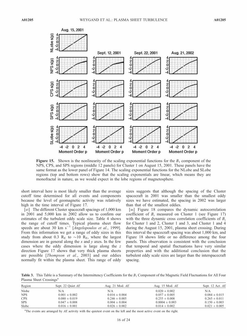
at p = 0. Note that using the method defined in Lui [2001]we rely only on the first few moments to determine theintermittency coefficient and do not need to determine thereliability of the higher moments [Horbury and Balogh,2004]. Using the same method, the intermittency coefficientfor the lower panel of Figure 14 is determined to be 0.057 ±0.005. This value is smaller than the intermittencycoefficient determined by Lui [2001]. The scaling expo-nential functions for the lobe and plasma sheet regions forall cases are shown in Figure 15. The purpose of this figureis to provide a qualitative comparison between the turbulentplasma sheet and the nonturbulent lobe as well as tocompare the different events. The format of Figure 15 is thesame as in lower panel of Figure 14. The black curvesrepresent the s(p) values and errors bars are plotted but notvisible. If the lobe region is not turbulent, then scaleinvariance applies, which implies a linear relationshipbetween s(p) and p. The curves in the lobe regions (topand bottom rows) in Figure 15, when plotted on the samescale as Figure 14 are nearly linear. This suggests the lobemagnetic field is monofractal as we expect. On the otherhand, the curves in all the plasma sheet regions shown inFigure 15 are at least somewhat nonlinear.[39] Table 3 contains the intermittency coefficients cal-

culated for each magnetotail region using the B1 componentof the magnetic field. Values of zero are consistent withnonturbulent fluctuations whereas values on the order of 0.2to 0.4 indicate that the regions are intermittently turbulent[Burlaga, 1993; Consolini et al., 1996]. Events in the tableare arranged by the AE activity as noted at the top of thecolumn. In each event the largest intermittency coefficientvalues occur in the CPS region. The largest intermittencycoefficient values found in the SPS and NPS regions werecalculated using observations from the most active day,September 12, 2001. In all the lobe regions a smallcoefficient value is determined. Table 3 only lists intermit-tency coefficient values for the B1 component, but similar

Figure 12. On the basis of Figure 8 this plot shows thekurtosis of the PDFs of the magnetic field fluctuations inthe Bx component. The horizontal dotted line indicates thekurtosis of a Gaussian distribution (i.e., 3). The verticalblack line identifies the plasma sheet ion gyroperiod.Notice that both the kurtoses determined in the southernlobe and northern lobe regions (the dark dashed gray andthe light dashed gray curves, respectively) remain close to�4 while the kurtoses for the plasma sheet regions aresubstantially higher for small values of t.


13 of 24

A01205

values exist for the other two components of the magneticfield in this coordinate system.

4.5. Autocorrelation and Cross Correlation

[40] In the previous sections we have analyzed the timeseries from a single spacecraft and found evidence thatintermittent turbulence is present within the plasma sheetmagnetic field. The underlying assumption of the analysisis that temporal fluctuations are equivalent to spatialfluctuations. In this section, we provide support for thatassumption by comparing (temporal) autocorrelations with(spatiotemporal) cross correlations of the magnetic field.We use the results to determine the scale size of theturbulent eddies in the magnetic field.[41] Autocorrelation, Ag, is defined as:

Ag tð Þ ¼

Zg tð Þ � gh i½ � g t þ tð Þ � gh i½ �dtffiffiffiffiffiffiffiffiffiffiffiffiffiffiffiffiffiffiffiffiffiffiffiffiffiffiffiffiffiffiffiffiffiffiffiffiffiffiffiffiffiffiffiffiffiffiffiffiffiffiffiffiffiffiffiffiffiffiffiffiffiffiffiffiffiffiffiffiffiffiffiffiffiffiffiffiffiffiffiffiffiffiffiffiffiffiffiffiffiffiZ

g tð Þ � gh i½ �dt� �2 Z

g t þ tð Þ � gh i½ �dt� �2

s ; ð9Þ

where hgi is the average value of g(t) in a data interval and tis the discrete time shift in seconds. The magnetic field willbe correlated with itself within a turbulent eddy anduncorrelated outside the eddy. The temporal scale size ofthe turbulent eddies is defined as the point at which theautocorrelation coefficient drops to 1/e (i.e., �0.37). Thisconservative definition of the eddy scale size is the sameone adopted by Borovsky et al. [1997], which makes acomparison between the studies easier.[42] Figure 16 shows plots of the autocorrelation coef-

ficients of the three components of the magnetic field andtheir magnitude for the CPS region on August 15, 2001,at discrete time shifts, t, of 1 s to 500 s. Note thatperiods of 5,000 s and longer were filtered out in order toremove long period fluctuations such as dipolarizationfluctuations associated with substorms. The 1/e cutofftime, t1/e, indicated with the dashed line, in the Bx

component is 116 s,for the By component it is 68 s,and for the Bz component it is 48 s. The three 1/e cutofftimes are distinctly different suggesting that the eddy’sshape may be oblong extended along the tail. Table 4

Figure 13. PDFs from August 21, 2002. The top row shows the unscaled PDFs of the fluctuations inthe square of the Btotal component of the magnetic field. The bottom row shows the rescaled PDFs. ThePDFs in the bottom row do not rescale to a single master curve as the solar wind PDFs do in Hnat et al.[2002]. See color version of this figure at back of this issue.


14 of 24

A01205

gives the 1/e cutoff time for all components in all regionsand in all regions for all four events. The t1/e times rangefrom 0.75 min to 46 min for four different events duringquiet, moderate, and active conditions. Borovsky et al.[1997] determined t1/e times of 6 min to 25 min. Themean cutoff time determined from all four events in all threeplasma sheet regions for all magnetic field components isabout 900 s.[43] The autocorrelation function allows us to identify the

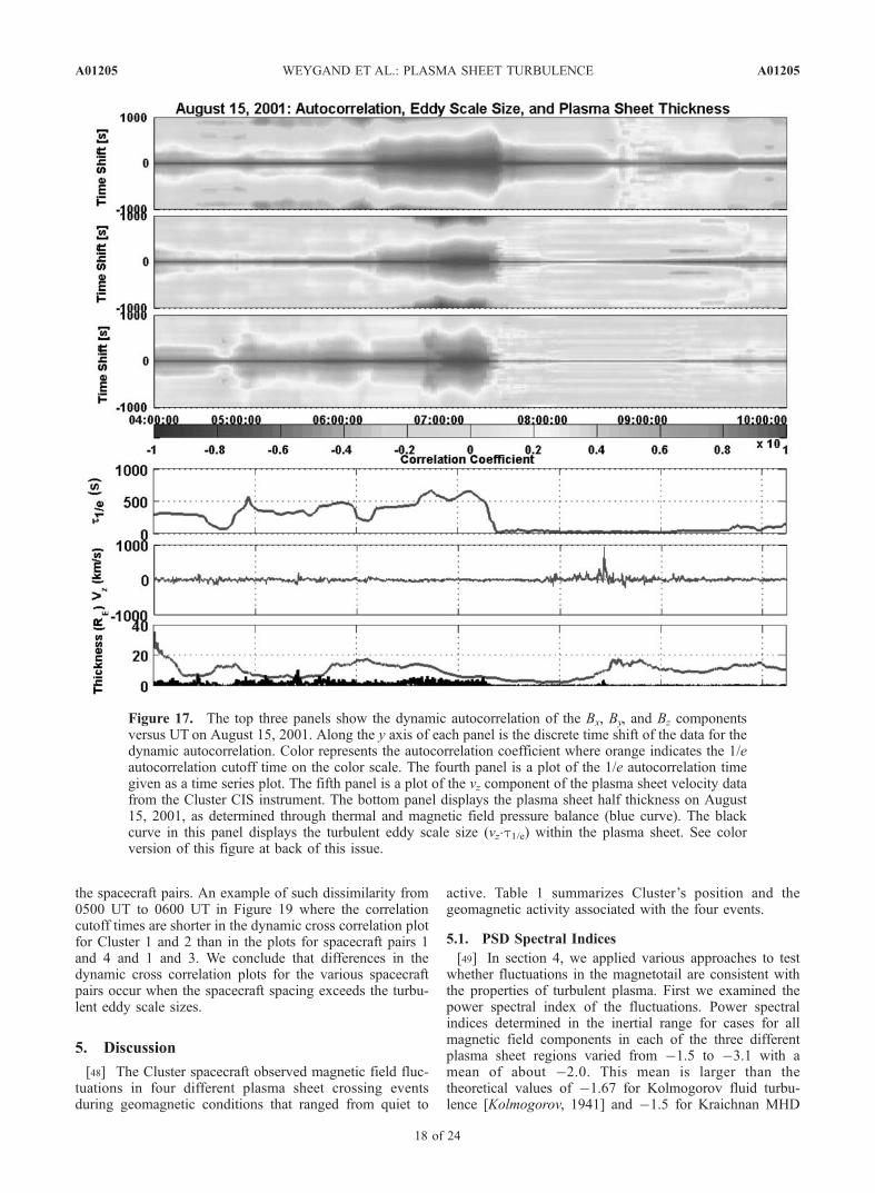
average time for an eddy to pass by the spacecraft. Possiblyof greater interest is to demonstrate the dynamic nature ofturbulent eddies passing the spacecraft. A dynamic auto-correlation allows us to identify the changing scale size ofeddies by examining portions of the time series data.Figure 17 shows the dynamic nature of the autocorrelationfor August 15, 2001, from about 0400 UT to 1000 UT(part of the NPS and the CPS) in all three components ofthe field in the GSM coordinate system. To create the topthree plots periods longer than 5000 s have been filteredout and an autocorrelation of the magnetic field timeseries is done over segments with time durations of1000s in length. The 1/e cutoff time corresponds approx-imately to the boundary between the orange and theyellow on the color scale. The 1/e cutoff time is moreclearly shown in the fifth panel and it varies with time,which suggests that the eddy scale sizes can change

significantly. The sixth panel gives the estimated plasmasheet thickness (blue curve) as determined by Thompsonet al. [2003]. The thickness was determined throughthermal and magnetic field pressure balance and a modelof the plasma sheet structure related to the Harris neutralsheet.[44] It is of interest to determine whether the inferred

plasma sheet thickness is sufficiently large that the estimatedspatial dimensions of the turbulent eddies fit within theplasma sheet. With the cutoff time and the flow speed ofthe plasma determined by the CIS instrument on Cluster(shown in the fourth panel of Figure 17) the turbulenteddy scale size can be estimated as Leddy = v�t1/e. Theeddy scale size is plotted as the black curve in the sixthpanel. The eddy scale size is smaller than the estimatedsize of the plasma sheet except during two 8 s periodsobserved at about 0525 UT. The data indicate that theeddy scale size decreases on average when the plasmasheet thickness decreases. An example of this decrease isshown just before the time of the substorm onset thatoccurred at 0751 UT. The mean cutoff time determinedfrom data plotted in panel 5 is about 230 s and the meaneddy scale size in the z direction is about 6,000 km, whichis similar to the average eddy scale sizes of 10,000 km and4,000 km determined by Borovsky et al. [1997] and Neaguet al. [2001], respectively. The mean cutoff time for the

Figure 14. Shown in the top panel is the structure function for the B1 component of the NPS region forCluster 1 on August 15, 2001. The inertial region is marked with the dashed horizontal line, and theintermittent turbulence region is demarcated in between the dash-dotted black vertical lines. The datapoints in the top panel for p = 4 (black curve), 3 (dark gray curve), and 2 (gray curve) have been shiftedup by a value of 9, 6, and 3 on the log scale in order to more clearly show all the data on one plot. Thelower panel shows a nonlinear relationship between s(p) and p where s(p) is the slope of the data in theintermittent turbulent region in the upper panel.


15 of 24

A01205

short interval here is most likely smaller than the averagecutoff time determined for all events and componentsbecause the level of geomagnetic activity was relativelyhigh in the time interval of Figure 17.[45] The different Cluster spacecraft spacings of 1,000 km

in 2001 and 5,000 km in 2002 allow us to confirm ourestimates of the turbulent eddy scale size. Table 4 showsthe range of cutoff times. Typical plasma sheet flowspeeds are about 30 km s�1 [Angelopoulos et al., 1999].From this information we get a range of eddy sizes in thisstudy from about 0.3 RE to �10 RE, where the largestdimension are in general along the x and y axes. In the fewcases where the eddy dimension is large along the zdirection Figure 17 shows that very thick plasma sheetsare possible [Thompson et al., 2003] and our eddiesnormally fit within the plasma sheet. This range of eddy

sizes suggests that although the spacing of the Clusterspacecraft in 2001 was smaller than the smallest eddysizes we have estimated, the spacing in 2002 was largerthan that of the smallest eddies.[46] Figure 18 compares the dynamic autocorrelation

coefficient of Bz measured on Cluster 1 (see Figure 17)with the three dynamic cross correlation coefficients of Bz

for Cluster 1 and 2, Cluster 1 and 3, and Cluster 1 and 4during the August 15, 2001, plasma sheet crossing. Duringthis interval the spacecraft spacing was about 1,000 km, andFigure 18 shows little or no difference among the fourpanels. This observation is consistent with the conclusionthat temporal and spatial fluctuations have very similarproperties and with the additional conclusion that theturbulent eddy scale sizes are larger than the interspacecraftspacing.

Figure 15. Shown is the nonlinearity of the scaling exponential functions for the B1 component of theNPS, CPS, and SPS regions (middle 12 panels) for Cluster 1 on August 15, 2001. These panels have thesame format as the lower panel of Figure 14. The scaling exponential functions for the NLobe and SLoberegions (top and bottom rows) show that the scaling exponentials are linear, which means they aremonofractal in nature, as we would expect in the lobe regions of magnetosphere.

Table 3. This Table is a Summary of the Intermittency Coefficients for the B1 Component of the Magnetic Field Fluctuations for All Four

Plasma Sheet Crossingsa

Region Sept. 22 Quiet AE Aug. 21 Mod. AE Aug. 15 Mod. AE Sept. 12 Act. AE

Nlobe N/A N/A 0.020 ± 0.002 N/ANPS 0.001 ± 0.002 0.016 ± 0.004 0.057 ± 0.005 0.084 ± 0.015CPS 0.080 ± 0.019 0.246 ± 0.005 0.255 ± 0.008 0.265 ± 0.011SPS 0.047 ± 0.008 0.004 ± 0.004 0.0004 ± 0.003 0.150 ± 0.003Slobe 0.016 ± 0.001 0.026 ± 0.002 0.014 ± 0.002 0.021 ± 0.005

aThe events are arranged by AE activity with the quietest event on the left and the most active event on the right.


16 of 24

A01205

[47] Figure 19, which has the same format as Figure 18,displays the dynamic autocorrelation and dynamic crosscorrelation data for the Bz component in the CPS crossingon August 21, 2002, when the spacecraft spacing was

roughly 5,000 km. This spacing is comparable with theminimum estimated size of the turbulent eddies. Thedynamic cross correlation does include intervals duringwhen there are differences in the cross correlations between

Figure 16. These four panels show the autocorrelation coefficient versus the discrete time shift t of thedata for the magnetic field components and the field magnitude observed in the CPS region between0754 UT and 1013 UT on August 15, 2001. The dashed line indicates the 1/e autocorrelation cutoff. The1/e autocorrelation cutoff time is given in each panel.

Table 4. Comparison of Autocorrelation Time (1/e) for Moderate, Quiet, and Active Plasma Sheet Crossings

Region Comp

August 15, 2001Moderate

September 12, 2001Quiet

September 22, 2001Active

August 21, 2002Active

UT t1/e s UT t1/e s UT t1/e S UT t1/e s

NPS Bx 0130–0754 956 0040–0453 1628 1004–1317 956 0000–0442 1108NPS By 668 2572 1348 712NPS Bz 1560 1824 1124 1124NPS Btotal 640 1400 632 532CPS Bx 0754–1013 116 0453–0638 468 1317–1426 656 0442–0921 132CPS By 68 216 824 120CPS Bz 48 48 1152 1236CPS Btotal 80 228 648 452SPS Bx 1013–1330 1376 0638–0742 1720 1426–2150 240 0921–1200 1524SPS By 384 244 548 120SPS Bz 460 1904 1856 244SPS Btotal 1336 1708 244 1476


17 of 24

A01205

the spacecraft pairs. An example of such dissimilarity from0500 UT to 0600 UT in Figure 19 where the correlationcutoff times are shorter in the dynamic cross correlation plotfor Cluster 1 and 2 than in the plots for spacecraft pairs 1and 4 and 1 and 3. We conclude that differences in thedynamic cross correlation plots for the various spacecraftpairs occur when the spacecraft spacing exceeds the turbu-lent eddy scale sizes.

5. Discussion

[48] The Cluster spacecraft observed magnetic field fluc-tuations in four different plasma sheet crossing eventsduring geomagnetic conditions that ranged from quiet to

active. Table 1 summarizes Cluster’s position and thegeomagnetic activity associated with the four events.

5.1. PSD Spectral Indices

[49] In section 4, we applied various approaches to testwhether fluctuations in the magnetotail are consistent withthe properties of turbulent plasma. First we examined thepower spectral index of the fluctuations. Power spectralindices determined in the inertial range for cases for allmagnetic field components in each of the three differentplasma sheet regions varied from �1.5 to �3.1 with amean of about �2.0. This mean is larger than thetheoretical values of �1.67 for Kolmogorov fluid turbu-lence [Kolmogorov, 1941] and �1.5 for Kraichnan MHD

Figure 17. The top three panels show the dynamic autocorrelation of the Bx, By, and Bz componentsversus UT on August 15, 2001. Along the y axis of each panel is the discrete time shift of the data for thedynamic autocorrelation. Color represents the autocorrelation coefficient where orange indicates the 1/eautocorrelation cutoff time on the color scale. The fourth panel is a plot of the 1/e autocorrelation timegiven as a time series plot. The fifth panel is a plot of the vz component of the plasma sheet velocity datafrom the Cluster CIS instrument. The bottom panel displays the plasma sheet half thickness on August15, 2001, as determined through thermal and magnetic field pressure balance (blue curve). The blackcurve in this panel displays the turbulent eddy scale size (vz�t1/e) within the plasma sheet. See colorversion of this figure at back of this issue.


18 of 24

A01205

plasma turbulence [Kraichnan, 1965]. However, the valuesdetermined in this study are similar to those of calculatedin Borovsky et al. [1997]: �1.6 to �3.0. Although thesevalues are consistent with earlier studies, they do notconvincingly demonstrate that turbulence is present inthe plasma sheet.[50] Spectral indices near �2 have also been found in

studies of the solar wind [Burlaga, 1991b]. Burlaga andMish [1987] and Roberts and Goldstein [1987] haveargued that the �2 spectral index found in the solar windmay arise if coherent power is present in large-amplitudelow-frequency fluctuations. These large-amplitude low-frequency fluctuations are related to shocks evolving inthe solar wind. Roberts and Goldstein [1987] demonstratewhen the large-amplitude fluctuations are removed, thenthe spectral index increases to approximately �5/3. Wethink that this interpretation does not apply to the fluctua-

tions in the plasma sheet where large-amplitude shocks orequivalent perturbations are not present. However, Chang etal. [2004], who model intermittent magnetic turbulentfluctuations in the plasma sheet region, also obtained aspectral index of �2. Their model produces intermittentfluctuations through coexisting nonpropagating spatiotem-poral fluctuations and propagating modes. If the nonpropa-gating spatiotemporal fluctuations are related to large-scalefluctuations such as flapping of the magnetotail, then thismay be a source of coherent power in large-amplitudelow-frequency fluctuations similar to those referred to byBurlaga and Mish [1987] and Roberts and Goldstein[1987]. This suggests that the nonpropagating fluctuationsare the source of the �2 spectral index. It would be ofinterest to examine the spectral index for each of theseparate modes in the Chang et al. [2004] model todetermine if the spectral index of �2 is dominated by one

Figure 18. The top panel is the dynamic autocorrelation for the Bz component of Cluster 1 on theAugust 15, 2001, in the NPS and CPS. The lower three panels are cross correlation coefficients betweenBz from Cluster 1 and Bz from the other three spacecraft. The format of the panels is the same as for theupper three panels in Figure 15. The spacing between the spacecraft is about 1000 km within the CPS,which is generally smaller than the turbulent eddy scale size. As a result, the dynamic autocorrelation andcross correlation panels look nearly identical. See color version of this figure at back of this issue.


19 of 24

A01205

component of the fluctuations or requires the combinationof both.[51] In subcategories based on regions, events, compo-

nents, plasma sheet plasma characteristics, solar windcharacteristics, and AE, the average spectral indices wereconsistent with �2 within the standard deviation. When thespectral indices are subdivided into components and plasmasheet regions, the average spectral index is again about�2 within the standard deviation for the B1 and B3

component, but �1.56 ± 0.04 for the B2 component. TheB2 component has the smallest spectral index for the NPSand SPS regions as well, but the standard deviationsassociated with these values are large and the valuesbecome nearly indistinguishable from the other two com-ponents. The B1 and B3 spectral indices of the CPS aremost likely larger than the B2 index due to tail flapping andsurface waves. These phenomena introduce additionalpower into the other two magnetic components, which

results in a more negative spectral index. The B2 compo-nent is not dramatically affected by tail flapping andsurface waves and little additional power is added to thosefluctuations. Thus its value (close to �1.5 representative ofpure MHD turbulence) is of particularly interesting.[52] We also obtained an average spectral index near �2

(representative of random fluctuations) in power spectra ofthe lobe regions. In some of the events there is reason tobelieve that the spacecraft repeatedly dipped into theplasma sheet during intervals in the nominal lobe region(see for example the Slobe region in Figure 5), the spectralindex of the lobe region may not have been accuratelyassessed in those cases so we will not offer any furtherinterpretation.

5.2. PDFs of Magnetic Field Fluctuations

[53] Next we looked at the PDFs of temporal fluctuationsat different time separations. We found that at the longest

Figure 19. The format of the panels is the same as in Figure 18. Data were acquired within the CPS,and the interspacecraft separation was about 5,000 km, which is close to the turbulent eddy scale size. Asa result, the dynamic autocorrelation and cross correlation panels show dissimilarities. For example, thecross correlation between C1 and C3 (third panel) is visibly different from the autocorrelation panel (toppanel) at about 0500 UT. See color version of this figure at back of this issue.


20 of 24

A01205

temporal separations considered (900 s), the distributionfunctions became approximately Gaussian in most cases.At shorter time separations the distribution functionsdiffered from Gaussian distributions with large fluctuationsrelatively more probable at short time separations. Wequantified the spread of the distribution functions byexamining the fourth moment of the distribution functions,the kurtosis. At short time separations, the kurtosis was 3, but in most regions, with increasing time separationsthe kurtosis approached 3, the value for a Gaussiandistribution. For crossings on August 15 and August 21the kurtosis in the CPS remained high at the largest valuesof the time separation.[54] We would expect the kurtosis to decrease to 3 when

t* becomes large enough that a typical eddy moves past thespacecraft in a time shorter than t*. It is possible that for thetwo cases in which the kurtosis remained high after 900 sthe turbulent eddies within the CPS filled such a largeregion of space that the spacecraft did not leave the eddywithin 900 s. The second possibility is that because geo-magnetic activity was high during these two events, thefluctuations were exceptionally large and lasted long, whencompared with the 900 s timescale. In fact, during the CPScrossing on August 15, 2001, a substorm was in progressduring most of the crossing.[55] Figures 8–11 all show non-self-similar scaling of

the PDFs with increasing temporal separation. The varia-tion of the PDFs with temporal separation presented here issimilar to the results of Sorriso-Valvo et al. [1999, 2001],which examined PDFs of solar wind flow and magneticfield fluctuations across much larger-scale sizes than thisstudy, but did not give the kurtosis associated with eachdistribution. The PDF scaling observed in this study is alsosimilar to the scaling of PDFs for flow fluctuationsobserved in fully developed turbulent shear flows createdin a laboratory system [Anselmet et al., 1984; Castaing etal., 1990].[56] Within the lobe regions the kurtoses are generally

less than 6.3 for all temporal separations. We do not believethat the lobe regions are turbulent but we have determinedthe kurtosis in the lobes as a means of comparison withplasma sheet distributions.[57] In another approach to the analysis of the PDFs of

the magnetic field fluctuation we applied the scaling func-tion outlined in Hnat et al. [2002] and given in equation (1).In the case that the fluctuations are monofractal, the rescal-ing of the PDFs should produce a single master curve. Wefound (Figure 13) that the rescaled PDFs do not lie on asingle master curve in the plasma sheet. As we pointedout in both section 4.3 a single scaling exponent did notappear to be present in log-log plots of P(0, t) versus t.This observation is consistent with the results from themultifractal analysis, which demonstrate that the scalingexponent is a nonlinear function of p.

5.3. Multifractal Analysis

[58] We tested anomalous scaling by use of equation (2).That test led to the conclusion that the fluctuations haveproperties similar to those found in the solar wind that areattributed to the presence of turbulence.[59] Lui [2001] examined the multifractal nature of sub-

storm-associated magnetic turbulence in the magnetotail at

kinetic scales. His study shows that the scaling exponentialsfor the square of the magnetic field fluctuations for all threecomponents in the VDH coordinate system are nonlinear asa function of the moment order and that this nonlinearityvaries with the distance from the neutral sheet. We found asimilar variation in the intermittency coefficient with dis-tance from the center of the plasma sheet. Lui states that hisresults provide evidence of cross-scale coupling and reor-ganization of auroral and magnetospheric phenomena,which support substorm models with multiscale processessuch as the current disruption model. However, it is notclear if this study is restricted to times when the spacecraftwas located within the plasma sheet.[60] Our results also are similar to but not easily

compared with the results previously observed whenexamining solar wind magnetic field fluctuations [Burlagaand Klein, 1986; Burlaga, 1991a, 1992]. Burlaga [1992]determined the s(p) data to be well fit with a cubicpolynomial for values of p between �15 and 15. Similarmultifractal results are observed within the solar windvelocity fluctuations. Burlaga [1993] and Tu and Marsch[1995] have shown that the s(p) function determined fromsolar wind velocity fluctuations is also nonlinear. None ofthese studies, except Burlaga [1993], evaluated the inter-mittency coefficient associated with the scaling exponen-tial functions. Burlaga [1991c, 1993] found intermittencycoefficients of 0.28 ± 0.27 and 0.19 ± 0.02, respectively,from multifractal analyses of solar wind velocity fluctua-tions. These values are similar to those obtained in thisstudy. The intermittency coefficients found in this studydetermined from the scaling exponential functions variedfrom 4�10�4 to 0.265.[61] Voros et al. [2003] have reported on the multiscaling

properties of the magnetic field fluctuations within burstybulk flow regions. They examined the Holder exponent,which is another measure of the ‘‘strength’’ of the bursti-ness, and the local intermittence measure at both small andlarge scales. From their analysis, Voros et al. [2003]concluded that while the fluctuations are a multiscalephenomena, the observed transitory and nonstationary na-ture of the fluctuations associated with the bursty bulk flowsprevents unambiguous support for a plasma sheet turbu-lence model.[62] In a related study, Consolini et al. [1996] examined

the structure of fluctuations in the auroral electrojet indexand found them to be multifractal. The intermittencycoefficient for the analysis is 0.400 ± 0.002. While it isinteresting to compare the intermittency coefficient ofConsolini et al. [1996] with our own, we do not expectto obtain the same values since AE is sensitive tofluctuations in the magnetic field vectors measured onthe ground while our study examines fluctuations in themagnetic field data observed in the magnetotail. It wouldbe interesting to determine the intermittency coefficientfor conjugate ground and space based magnetic fieldobservations to see if similar intermittency coefficientsare present.[63] All of these studies examine the multifractal nature

of the magnetic field or flow fluctuations, but none examinethe multifractal nature in the MHD inertial region. Ourmultifractal analysis reveals nonlinear scaling exponentialsfor the magnetic field fluctuations observed in the plasma


21 of 24

A01205

sheet region suggesting that the plasma there is intermit-tently turbulent. The strength of this intermittent turbulenceis characterized by the intermittency coefficient, which islargest in the CPS region during moderate to active times.The value of the intermittency coefficient decreases withincreasing distance from the center of the plasma sheet (i.e.,in the NPS and SPS regions) and with decreasing AEactivity.[64] We have stated that we expect the magnetotail lobe

regions to be nonturbulent and the PDFs of the magneticfield fluctuations appear to support this idea. However, theintermittency coefficient determined for the lobe regions isnonzero within the uncertainty. In fact, the coefficient islarger than some values determined within the NPS andSPS regions. The nonzero coefficient may suggest thatthese regions are multifractal in nature, but the valuesdetermined in this study are considerably lower than anypreviously reported values. Furthermore, there is no evi-dence for the presence of strong instabilities in the loberegions to generate turbulent fluctuations. As an additionalcheck, we generated a times series of 100,000 points ofnormally distributed random fluctuations with approxi-mately the same amplitude and uncertainty as those inthe plasma sheet. The intermittency coefficient for thistime series was calculated to be zero within the uncertainty.We hypothesize that solar wind and plasma sheet activitydrives the lobe regions and generates some of the lobefluctuations, but further works needs to be done to confirmthis hypothesis.

5.4. Autocorrelation and Dynamic Cross Correlation

[65] Finally, we looked at dynamic autocorrelations ofdata from a single spacecraft and compared them with thecross correlation of data measured simultaneously at twodifferent spacecraft. By using data from both 2001 (meanspacing near 1,000 km) and 2002 (mean spacing near5,000 km), we found that the cross correlations for thelong and short spatial separations were significantly differ-ent. With short separations, the cross correlations wereindistinguishable for all pairs of spacecraft and were verysimilar to the autocorrelations. With large separations,differences among the cross correlations for different space-craft pairs were intermittently observed. This suggests thatwhen the separation between some pairs of spacecraftexceeded the typical size of the turbulent eddies thecorrelations were absent, but when the spatial separationsbetween spacecraft pairs was smaller than the scale of theturbulent eddies some correlation was present. These resultsare consistent if we assume that one can apply the ‘‘Taylorhypothesis’’ to the plasma sheet despite the fact that flowsare sub-Alfvenic. However, we point out that the dynamiccross correlation never truly separates temporal fluctuationsfrom spatial fluctuations because the dynamic cross corre-lation is based on use of a short window to sample the timeseries.[66] During the 2002 plasma sheet crossing season

some dynamic cross correlations showed few correlationcoefficients above 1/e (see the bottom panel of Figure 19at approximately 0810 UT), which means that the turbu-lent eddies were occasionally as small as �0.8 RE. For allfour cases the autocorrelation and cross correlation resultsshow that the eddy scale sizes are consistent with the

work of Borovsky et al. [1997] and Neagu et al. [2001],who found eddy scale sizes from about 4,000 km to10,000 km. The mean eddy scale size found in this studyis 6,000 km.

6. Summary and Conclusions

[67] This study has shown that the magnetic fluctuationsare consistent with expectations for an intermittentlyturbulent MHD fluid. Spectral indices near �2 weretypical, but a value of �1.56 was found for the approx-imately azimuthal component in the CPS. We speculatethat plasma sheet motion contributes to the B1 and B3

fluctuations (roughly radial and north-south) and that thevalue of �1.56 found for the B2 component may providethe most meaningful approximation to the spectral index inthe plasma sheet frame. It is interesting that the value isclose to the �1.5 expected for MHD plasma turbulence[Kraichnan, 1965].[68] The normalized PDFs of the magnetic field fluctua-

tions clearly indicate a significant variation in the kurtosisover a large range of temporal scale sizes. The kurtosistended to decrease from large values at the dissipation range(smallest scale sizes) to values close to 3 at large-scale sizes(larger than eddy scale sizes) in the inertial range of thefluctuations. The kurtosis is 6 and generally largest atsmall scales (heating scales) in the plasma sheet, �3 at largescales (convection scales) in the plasma sheet, and generally<6 at all scales in the lobe. The kurtosis remains fairly large(3 < kurtosis < 7) even at convection scale sizes within thecentral plasma sheet. Scaling behavior of PDFs in theplasma sheet is similar to that found for the solar wind[Sorriso-Valvo et al., 1999, 2001] and similar to what isobserved in intermittent turbulence [Carbone et al., 2002].[69] Attempts to rescale the PDFs to a single master curve

using the method outlined by Hnat et al. [2002] were notsuccessful. This suggests that the magnetic field fluctuationsare not monofractal as a constant scaling exponential wouldsuggest, but rather that the fluctuation are multifractal. Thisresult is supported by the findings presented here frommultifractal analysis.[70] The scaling exponential functions constructed for the

different plasma sheet regions are similar to the turbulentmagnetic field fluctuations reported by Lui [2001] at kineticscales, similar to the scaling exponential function for the AEindex data of Consolini et al. [1996], and similar to solarwind magnetic field multifractal structures [Burlaga andKlein, 1986; Burlaga, 1991a, 1992]. In these cases thescaling exponential functions are determined to be nonlinearas a function of the power of the ensemble average, p.The intermittency coefficients determined from the scalingexponential functions ranged from 4�10�4 to 0.265. Thecoefficients are largest in the CPS region during periodsof moderate to active AE and smallest in the NPS andSPS regions. Furthermore, the intermittency coefficientvalues are nonzero in the lobe regions possibly due todriving from the plasma sheet and solar wind.[71] Finally, the eddy scale sizes were determined through

autocorrelation and dynamic autocorrelation. The meaneddy scale size was identified to be as about 6,000 km witha mean autocorrelation cutoff time of 230 s for the August15, 2001, event. However, for all four events the mean


22 of 24

A01205

cutoff time was 900 s. During periods of nominal flow thistranslates to eddies on the order of 27,000 km, but, as wasshown in section 4.5, the eddy scale size varies significantlywith the correlation cutoff time and flow speed. Nearly alleddies easily fit within the plasma sheet and some eddiesmarginally fit except for several seconds of data. Theautocorrelation results for 2001 with spacecraft separationsof 1,000 km are consistent with cross correlation resultsdetermined in 2002 when the spacecraft spatial separationincreased to 5,000 km. The eddy scale sizes are alsoconsistent with the work of Borovsky et al. [1997] andNeagu et al. [2001], who found eddy scale sizes from about4000 km to 10,000 km. An examination of individualcomponents of the field indicates that eddies are oblongwith the longest length in the parallel magnetic fielddirection that is generally oriented along the tail axis withthe smallest length in the z direction.[72] The similarity of the quantitative results of this study

found for the magnetotail with those found for the solarwind leads one to ask whether the fluctuations of the plasmasheet magnetic field are directly driven by the fluctuationsin the solar wind. Our analysis raises this question withoutproviding the answer.

[73] Acknowledgments. This work was supported by NASA grantNAG5-12131. We would also like to thank W. Zhou, I. Zaliapin, S. Joy,R. Walker, J. Green, R. Silva, and M. B. Moldwin for their advice inevaluating this work.[74] Arthur Richmond thanks Tom Tien Sun Chang and Zoltan Voros

for their assistance in evaluating this paper.

ReferencesAngelopoulos, V., T. Mukai, and S. Kokubun (1999), Evidence of inter-mittency in Earth’s plasma sheet and implications for self-organizedcriticality, Phys. Plasmas, 6, 4161–4168.

Anselmet, F., Y. Gagne, E. J. Hopfinger, and R. A. Antonia (1984), High-order velocity structure functions in turbulent shear flows, J. Fluid Mech.,140, 63–89.

Antonia, R. A., B. R. Satyaprakash, and A. K. M. F. Hussain (1982),Statistics of fine-scale velocity in turbulent plane and circular jets,J. Fluid Mech., 119, 55–89.

Balogh, A., et al. (1997), The Cluster magnetic field investigation, SpaceSci. Rev., 79, 65–91.

Borovsky, J. E., and H. O. Funsten (2003), MHD turbulence in the Earth’splasma sheet: Dynamics, dissipation, and driving, J. Geophys. Res.,108(A7), 1284, doi:10.1029/2002JA009625.

Borovsky, J. E., R. C. Elphic, H. O. Funsten, and M. F. Thomsen (1997),The Earth’s plasma sheet as a laboratory for turbulence in high-betaMHD, J. Plasma Phys., 57, 1–34.

Burlaga, L. F. (1991a), Multifractal structure of the interplanetary magneticfield: Voyager 2 observations near 25 AU, 1987–1988, Geophys. Res.Lett., 18, 69–72.

Burlaga, L. F. (1991b), Multifractal structure of speed fluctuations inrecurrent streams at 1 AU and near 6 AU, Geophys. Res. Lett., 18,1651–1654.

Burlaga, L. F. (1991c), Intermittent turbulence in the solar wind, J. Geo-phys. Res., 96, 5947–5951.

Burlaga, L. F. (1992), Multifractal structure of the magnetic field andplasma in recurrent streams at 1 AU, J. Geophys. Res., 97, 4283–4293.

Burlaga, L. F. (1993), Intermittent turbulence in large-scale velocity fluc-tuations at 1 AU near solar maximum, J. Geophys. Res., 98, 17,467–17,473.

Burlaga, L. F., and L. W. Klein (1986), Fractal structure of the interplane-tary magnetic field, J. Geophys. Res., 91, 347–350.

Burlaga, L. F., and W. H. Mish (1987), Large-scale fluctuations in theinterplanetary medium, J. Geophys. Res., 92, 1261–1266.

Carbone, V., et al. (2002), To what extent can dynamical models describestatistical features of turbulent flow, Europhysics, 58, 349–355.

Castaing, B., Y. Gagne, and E. J. Hopfinger (1990), Velocity probabilitydistribution functions of high Reynolds number turbulence, Physica D,46, 177–200.

Chang, T. (1999), Self-organized criticality, multi-fractal spectra, sporadiclocalized reconnections and intermittent turbulence in the magnetotail,Phys. Plasmas, 6, 4137–4145.

Chang, T., S. W. Y. Tam, and C.-C. Wu (2004), Complexity induced aniso-tropic bimodal intermittent turbulence in space plasma, Phys. Plasmas,11, 1287–1299.

Coleman, P. (1968), Turbulence, viscosity, and dissipation in the solar windplasma, Astrophys. J., 153, 371.

Consolini, G., M. F. Marcucci, and M. Candidi (1996), Multifractal struc-tures of auroral electrojet index data, Phys. Rev. Lett., 76, 4082–4085.

Goldstein, M. L., and D. A. Roberts (1999), Magnetohydrodynamic turbu-lence in the solar wind, Phys. Plasma, 6, 4154–4159.

Goldstein, M. L., D. A. Roberts, and W. H. Matthaeus (1995), Magnetohy-drodynamic turbulence in the solar wind, Ann. Rev. Astron. Astrophys.,33, 283–325.

Goldstein, M. L., D. A. Roberts, and W. H. Matthaeus (1997), Magnetohy-drodynamic turbulence in cosmic winds, in Cosmic Winds and theHeliosphere, edited by J. R. Jokipii, C. P. Sonett, and M. S. Giampapa,pp. 521–579, Univ. of Ariz. Press, Tucson.

Hnat, B., S. C. Chapman, G. Rowlands, N. W. Watkins, and W. M. Farrell(2002), Finite size scaling in the solar wind magnetic field energy densityas seen by WIND, Geophys. Res. Lett., 29(10), 1446, doi:10.1029/2001GL014587.

Horbury, T. S., and A. Balogh (2004), Structure function measurements ofthe intermittent MHD turbulent cascade, Nonlinear Processes Geophys.,4, 185–199.

Kadomtsev, B. (1965), Plasma Turbulence, Elsevier, New York.Klimas, A. J., J. A. Valdivia, D. Vassiliadis, D. N. Baker, M. Hesse, andJ. Takalo (2000), Self-organized criticality in the storm phenomenonand its relation to localized reconnection in the magnetospheric plasmasheet, J. Geophys. Res., 105, 18,765–18,780.

Kolmogorov, A. N. (1941), The local structure of turbulence in incompres-sible viscous fluid for very large Reynolds’ numbers, Dokl. Akad. NaukSSSR, 30, 301–305.

Kraichnan, R. H. (1965), Inertial range of hydromagnetic turbulence, Phys.Fluids, 8, 1385–1387.

Leung, P. T., and C. H. Gibson (2005), Turbulence and fossil turbulence inoceans and lakes, Chin. J. Oceanol. Limnol., in press.

Lui, A. T. Y. (2001), Multifractal and intermittent nature of substorm-associated magnetic turbulence in the magnetotail, J. Atmos. Sol. Terr.Phys., 63, 1379–1385.

Lui, A. T. Y. (2002), Multiscale phenomena in the near-Earth magneto-sphere, J. Atmos. Sol. Terr. Phys., 64, 125–143.

L’vov, V. S., and I. Procaccia (1998), Computing the scaling exponents influid turbulence from first principles: The formal setup, Physica A, 257,165–196.

Matthaeus, W. H., and M. L. Goldstein (1982), Measurements of the ruggedinvariants of magnetohydrodynamic turbulence in the solar wind, J. Geo-phys. Res., 87, 6011–6028.

McPherron, R. L., et al. (2002), A comparison of Cluster observations ofthe tail current during substorms and quiet times, Eos Trans. AGU,83(47), Fall Meet. Suppl., SM71A-0574.

Meneveau, C., and K. R. Sreenivasan (1991), The multifractal nature ofturbulent energy dissipation, J. Fluid Mech., 224, 429–484.

Naert, A., L. Puech, B. Chabaud, J. Peinke, B. Castaing, and B. Hebral(1994), Velocity intermittency in turbulence—How to objectively char-acterize it, J. Phys. Ii, 4, 215–224.

Neagu, E., S. P. Gary, J. E. Borovsky, W. Baumjohann, and R. A. Treumann(2001), Constraints on magnetic fluctuation energies in the plasma sheet,Geophys. Res. Lett., 28, 919–922.

Paladin, G., and A. Vulpiani (1987), Anomalous scaling law in multifractalobjects, Phys. Rep., 156, 147.

Reme, H., et al. (1997), The Cluster ion spectrometry (CIS) experiment,Space Sci. Rev., 79, 303–350.

Roberts, D. A., and M. L. Goldstein (1987), Spectral signatures of jumpsand turbulence in interplanetary speed and magnetic field data, J. Geo-phys. Res., 92, 10,105–10,110.

Sorriso-Valvo, L., V. Carbone, and P. Veltri (1999), Intermittency in thesolar wind turbulence through probability distribution functions of fluc-tuations, Geophys. Res. Lett., 26, 1801–1804.

Sorriso-Valvo, L., V. Carbone, P. Giuliani, P. Veltri, R. Bruno, V. Antoni,and E. Martines (2001), Intermittency in plasma turbulence, Planet.Space Sci., 49, 1193–1200.

Thompson, S., M. G. Kivelson, K. K. Khurana, R. L. McPherron,A. Balogh, H. Reme, L. M. Kistler, and J. M. Weygand (2003), Multi-spacecraft studies of the structure and dynamics of the magnetotailcurrent sheet, in Geophysical Research Abstracts [CD-ROM], vol. 5,Eur. Geophys. Union, Nice, France, April.

Tu, C.-Y., and E. Marsch (1995), MHD structures, waves and turbulence inthe solar wind: Observations and theories, Space Sci. Rev., 73, 1–210.


23 of 24

A01205

Voros, Z., et al. (2003), Multi-scale magnetic field intermittence in theplasma sheet, Ann. Geophys., 21, 1955–1964.

��A. Balogh, Imperial College of Science and Technology, London SW7

2BZ, UK.J. Borovsky, Los Alamos National Laboratory, Los Alamos, NM 87545,

USA.

M. L. Goldstein and D. A. Roberts, Goddard Space Flight Center,Greenbelt, MD 20771, USA.K. K. Khurana, M. G. Kivelson, R. L. McPherron, H. K. Schwarzl, S. M.

Thompson, and J. M. Weygand, Institute of Geophysics and PlanetaryPhysics, University of California, Los Angeles, CA 90095-1567, USA.( [email protected])L. M. Kistler, Institute for the Study of Earth, Oceans, and Space,

University of New Hampshire, Durham, NH 03824, USA.


24 of 24

A01205

Figure 2. Magnetic field time series data for August 15, 2001, from 0730 UT to 0830 UT for all fourspacecraft plotted versus universal time. The format is the same as Figure 1. Color is used to distinguishdata from the different Cluster spacecraft: black for Cluster 1, red for Cluster 2, green for Cluster 3, andblue for Cluster 4.

A01205 WEYGAND ET AL.: PLASMA SHEET TURBULENCE A01205

5 of 24

Figure 13. PDFs from August 21, 2002. The top row shows the unscaled PDFs of the fluctuations inthe square of the Btotal component of the magnetic field. The bottom row shows the rescaled PDFs. ThePDFs in the bottom row do not rescale to a single master curve as the solar wind PDFs do in Hnat et al.[2002].


14 of 24

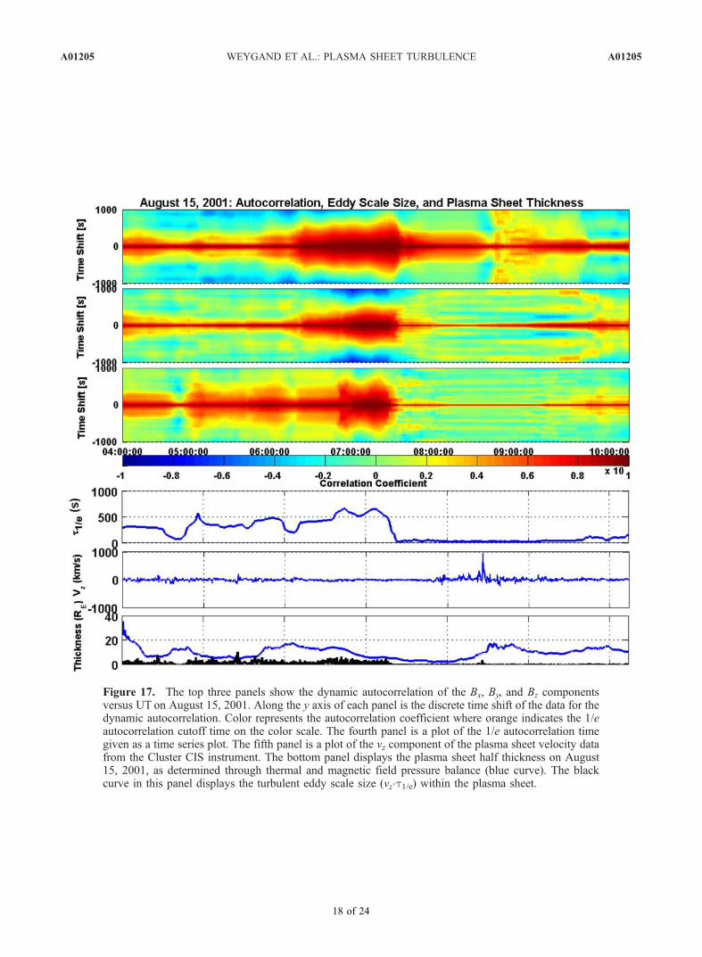
Figure 17. The top three panels show the dynamic autocorrelation of the Bx, By, and Bz componentsversus UT on August 15, 2001. Along the y axis of each panel is the discrete time shift of the data for thedynamic autocorrelation. Color represents the autocorrelation coefficient where orange indicates the 1/eautocorrelation cutoff time on the color scale. The fourth panel is a plot of the 1/e autocorrelation timegiven as a time series plot. The fifth panel is a plot of the vz component of the plasma sheet velocity datafrom the Cluster CIS instrument. The bottom panel displays the plasma sheet half thickness on August15, 2001, as determined through thermal and magnetic field pressure balance (blue curve). The blackcurve in this panel displays the turbulent eddy scale size (vz�t1/e) within the plasma sheet.


18 of 24

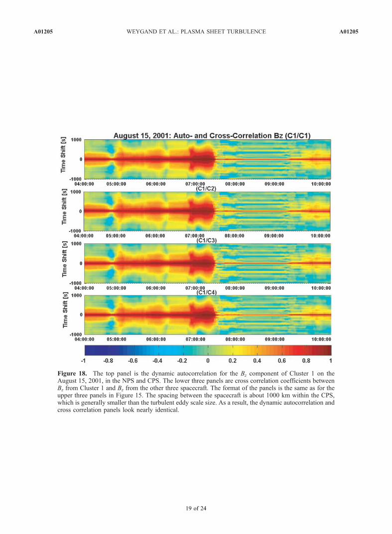
Figure 18. The top panel is the dynamic autocorrelation for the Bz component of Cluster 1 on theAugust 15, 2001, in the NPS and CPS. The lower three panels are cross correlation coefficients betweenBz from Cluster 1 and Bz from the other three spacecraft. The format of the panels is the same as for theupper three panels in Figure 15. The spacing between the spacecraft is about 1000 km within the CPS,which is generally smaller than the turbulent eddy scale size. As a result, the dynamic autocorrelation andcross correlation panels look nearly identical.


19 of 24

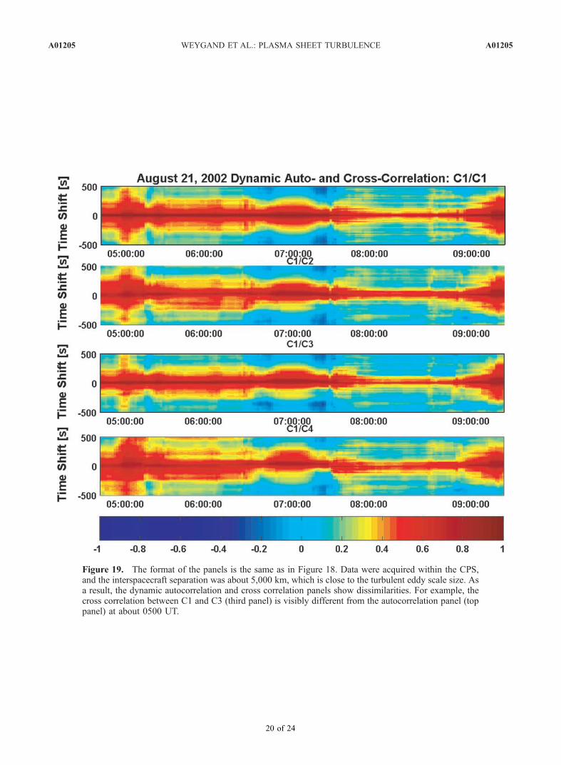
Figure 19. The format of the panels is the same as in Figure 18. Data were acquired within the CPS,and the interspacecraft separation was about 5,000 km, which is close to the turbulent eddy scale size. Asa result, the dynamic autocorrelation and cross correlation panels show dissimilarities. For example, thecross correlation between C1 and C3 (third panel) is visibly different from the autocorrelation panel (toppanel) at about 0500 UT.


20 of 24

plasma sheet turbulence observed by cluster ii

Documents