HAL Id: hal-01613581https://hal.archives-ouvertes.fr/hal-01613581

Submitted on 9 Oct 2017

HAL is a multi-disciplinary open accessarchive for the deposit and dissemination of sci-entific research documents, whether they are pub-lished or not. The documents may come fromteaching and research institutions in France orabroad, or from public or private research centers.

L’archive ouverte pluridisciplinaire HAL, estdestinée au dépôt et à la diffusion de documentsscientifiques de niveau recherche, publiés ou non,émanant des établissements d’enseignement et derecherche français ou étrangers, des laboratoirespublics ou privés.

Plasma Lab Statistical Model Checker: Architecture,Usage and Extension

Axel Legay, Louis-Marie Traonouez

To cite this version:Axel Legay, Louis-Marie Traonouez. Plasma Lab Statistical Model Checker: Architecture, Usage andExtension. SOFSEM 2017 - 43rd International Conference on Current Trends in Theory and Practiceof Computer Science, Jan 2017, Limerick, Ireland. <hal-01613581>

Plasma Lab Statistical Model Checker:Architecture, Usage and Extension

Axel Legay and Louis-Marie Traonouez

Inria, Rennes, France

Abstract. Plasma Lab is a modular statistical model checking (SMC)platform that facilitates multiple SMC algorithms and multiple mod-elling and query languages. Plasma Lab may be used as a stand-alonetool with a graphical development environment or invoked from the com-mand line for high performance scripting applications. This tutorial firstpresents an overview of Plasma Lab architecture, modelling languagesand algorithms. Then we present the usage of the tool to design modelsand perform various experiments Finally we propose a tutorial on howto develop a new plugin for Plasma Lab.

1 Introduction

Statistical model checking (SMC) employs Monte Carlo methods to avoid thestate explosion problem of probabilistic (numerical) model checking. To estimateprobabilities or rewards, SMC typically uses a number of statistically indepen-dent stochastic simulation traces of a discrete event model. Being independent,the traces may be generated on different machines, so SMC can efficiently ex-ploit parallel computation. Reachable states are generated on the fly and SMCtends to scale polynomially with respect to system description. Properties maybe specified in bounded versions of the same temporal logics used in probabilis-tic model checking. Since SMC is applied to finite traces, it is also possible touse logics and functions that would be intractable or undecidable for numeri-cal techniques. In recent times, dedicated SMC tools, such as YMER1, VESPA,APMC2 and COSMOS3, have been joined by statistical extensions of establishedtools such as PRISM4, UPPAAL5 and MRMC6. In this work we describe PlasmaLab7, a modular Platform for Learning and Advanced Statistical Model checkingAlgorithms [2].

SMC approximates the probabilistic model checking problem by estimatingthe parameter of a Bernoulli random variable, for which there are well definedconfidence bounds (e.g., [10]). The general principle is to simulate the modelor system in order to generate execution traces. These traces are checked withrespect to a logic such as Bounded Linear Temporal Logic (BLTL) [1] and theresults are combined with statistical techniques.

1 www.tempastic.org/ymer/ 2 http://archive.is/OKwMY3 www.lsv.ens-cachan.fr/~barbot/cosmos/

4 www.prismmodelchecker.org5 www.uppaal.org 6 www.mrmc-tool.org 7 https://project.inria.fr/plasma-lab/

BLTL restricts the classical Linear Temporal Logic by bounding the scope ofthe temporal operators. Syntactically, we have

ϕ,ϕ′ := true | P | ϕ ∧ ϕ′ | ¬ϕ | X≤t | ϕ U≤t ϕ′,

where ϕ,ϕ′ are BLTL formulas, t ∈ Q≥0, and P is an atomic proposition thatis valid in some state. As usual, we define F≤tϕ ≡ true U≤tϕ and G≤tϕ ≡¬F≤t¬ϕ. The semantics of BLTL, presented in Table 1, is defined with respectto an execution trace ω = (s0, t0), (s1, t1), . . . , (sn, tn) of the system, where eachstate (si, ti) comprises a discrete state si and a time ti ∈ R≥0. We denote byωi = (si, ti), . . . , (sn, tn) the suffix of ω starting at step i.

ω |= X≤t ϕ iff ∃i, i = max{j | t0 ≤ tj ≤ t0 + t} and ωi |= ϕ

ω |= ϕ1 U≤t ϕ2 iff ∃i, t0 ≤ ti ≤ t0 + t and ωi |= ϕ2 and ∀j, 0 ≤ j < i, ωj |= ϕ1

ω |= ϕ1 ∧ ϕ2 iff ω |= ϕ1 and ω |= ϕ2 ω |= ¬ϕ iff ω 6|= ϕ

ω |= P iff si |= P ω |= true

Table 1: Semantics of BLTL.

Plasma Lab implements qualitative and quantitative SMC algorithms. Quan-titative algorithms decide between two contrary hypothesis (e.g, is the proba-bility to satisfy the requirement is above a given threshold), while quantitativetechniques compute an estimation of a stochastic measure (e.g., the probabilityto satisfy a property).

The “crude” Monte Carlo algorithm is a quantitative technique that uses Nsimulation traces ωi, i ∈ {1, . . . , N}, to calculate γ̃ =

∑Ni=1 1(ωi |= ϕ)/N , an

estimate of the probability γ that the system satisfies a logical formula ϕ, where1(·) is an indicator function that returns 1 if its argument is true and 0 other-wise. Using the Chernoff-Hoeffding bound [10], setting N =

⌈(ln 2− ln δ)/(2ε2)

⌉guarantees the probability of error is Pr(| γ̃− γ |≥ ε) ≤ δ, where ε and δ are theprecision and the confidence, respectively.

2 Plasma Lab Architecture

One of the main differences between Plasma Lab and other SMC tools is thatPlasma Lab proposes an API abstraction of the concepts of stochastic modelsimulator, property checker (monitoring) and SMC algorithm. In other words,the tool has been designed to be capable of using external simulators or inputlanguages. This not only reduces the effort of integrating new algorithms, butalso allows us to create direct plug-in interfaces with standard modelling andsimulation tools used by industry. The latter being done without using extracompilers.

The tool architecture is displayed in Fig. 1. The core of Plasma Lab is a light-weight controller that manages the experiments and the distribution mechanism.

Application-specificlogics

Application-specificlogics

Application-specificmodeling languagesApplication-specificmodeling languages

SMC algorithmsSMC algorithms

Distributionand management

Distributionand management

Fig. 1: Plasma Lab architecture.

It implements an API that allows to control the experiments either through userinterfaces or through external tools. It loads three types of plugins: 1. algorithms,2. checkers, and 3. simulators. These plugins communicate with each other andwith the controller through the API. Only a few classes must be implementedto extend the tool with custom plugins for adding new languages or checkers.

An SMC algorithm collects samples obtained from a checker component. Thechecker asks the simulator to initialize a new trace. Then, it controls the simu-lation by requesting new states, with a state on demand approach: new statesare generated only when needed to decide the property. Depending on the prop-erty language, the checker either returns Boolean or numerical values. Finally,the algorithm notifies the progress and sends the results through the controllerAPI. Plasma Lab offers several advanced SMC algorithms that can be applied tovarious models, including SMC algorithms for rare events and nondeterministicmodels.

Tables 2,3,4 presents the list of simulator, checker and algorithms plugins cur-rently available with Plasma Lab. Plasma Lab has also been used to verify othertypes of models through a connection or an integration with other tools.

3 Tool Usage

Plasma Lab also includes several user interfaces capable of launching SMC exper-iments through the controller API, either as standalone applications or integratedwith external tools:

RML Reactive Module Language: input language of the tool Prismfor Markov chains models

RML Adaptive Extension of RML for adaptive systems

Bio Biological language for writing chemical reactions

Matlab Session Allows to control the simulator of Matlab/Simulink

SystemC Simulation of SystemC models. The plugin requires an exter-nal tool (MAG, https://project.inria.fr/pscv/) to in-strument SystemC models and generate a C++ executableused by the plugin.

Table 2: Plasma Lab simulators

BLTL Bounded Linear Temporal Logic

ALTL Adaptive Linear Temporal Logic, and extension of BLTLwith new operators for adaptive systems

GSCL Goal and Contract Specification Language, a high level spec-ification language for systems of systems

Nested BLTL checker enhanced with nested probability operator

RML Observer A plugin that allows to write requirement as observers usinga language similar to RML. It is used to write rare properties.

Table 3: Plasma Lab checkers

Monte Carlo Monte Carlo probability estimation with Chernoff-Hoeffdingbound [10].

SPRT Sequential Probability Ratio Test for hypothesis testing [11].

Importance splitting Estimate the probability of rare events using the importancesplitting technique [5,6,7] to decompose a requirement withlow probability into a product of higher conditional proba-bilities that are easier to estimate.

Importance samplingwith cross entropy

Estimate the probability of rare events using importancesampling [4], to weight the probability distribution of theoriginal system to favour the rare event, and cross entropy,to determine an optimal weighted distribution.

SMC fornondeterministic

models

“Smart sampling” algorithms [3,9] to estimate minimum andmaximum probabilities in non deterministic models.

Table 4: Plasma Lab algorithms

– Plasma Lab Graphical User Interface (GUI). This is the main interface ofPlasma Lab. It incorporates all the functionalities of Plasma Lab and allowsto open and edit PLASMA project files.

– Plasma Lab Command Line (CLI). A terminal interface for Plasma Lab,with experiment and simulation functionalities, that allows to incorporatePlasma Lab algorithms into high performance scripting applications.

– Plasma Lab Service. A graphical or terminal interface for Plasma Lab dis-tributed service. Its purpose is to be deployed on a remote computer to rundistributed experiments, in connection with the Plasma Lab main interface.

– PLASMA2Simulink. This is a small “App” running from Matlab that allowsto launch Plasma Lab SMC algorithms directly from Simulink.

We present the usage of the GUI to design a RML model, simulate it andverify a BLTL requirement. We also present the commands of the CLI thatperform the same experiments. The GUI is composed of several panels that allow(i) to load, create and edit projects that comprise models and requirements,(ii) to perform simulations and debugging step-by-step, and (iii) to performvarious forms of SMC experimentation and optimization, either locally or usingdistributed algorithms.

3.1 Modelling

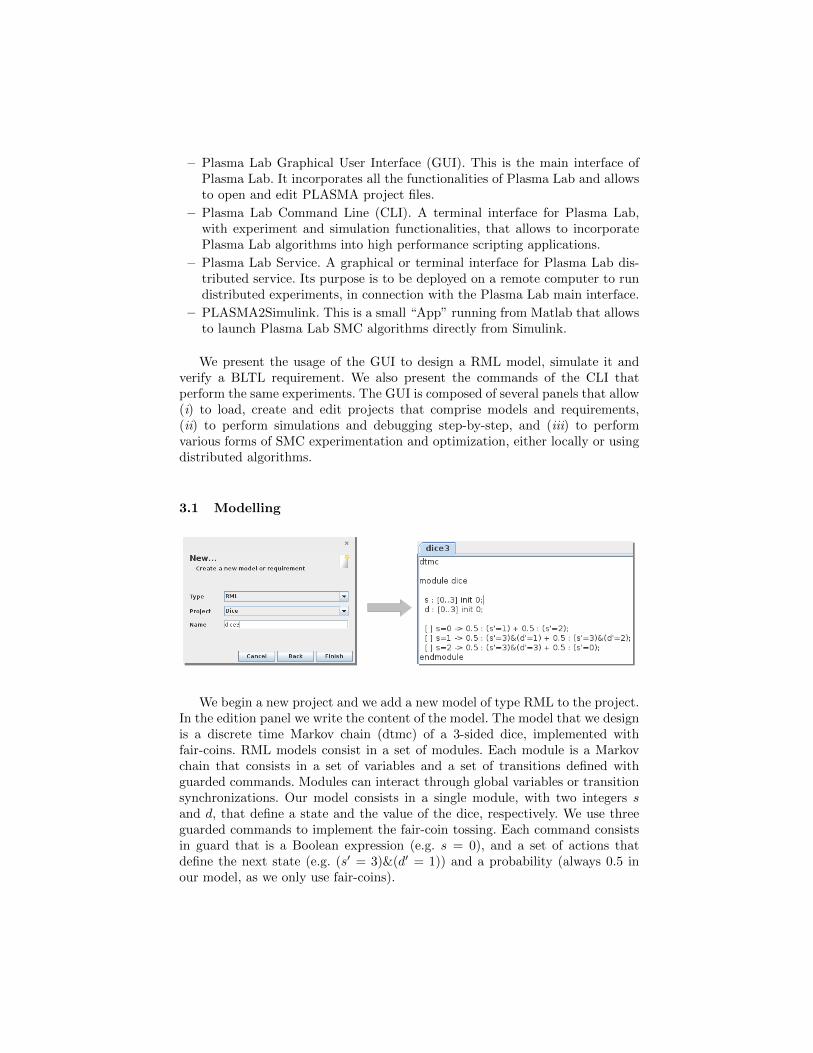
We begin a new project and we add a new model of type RML to the project.In the edition panel we write the content of the model. The model that we designis a discrete time Markov chain (dtmc) of a 3-sided dice, implemented withfair-coins. RML models consist in a set of modules. Each module is a Markovchain that consists in a set of variables and a set of transitions defined withguarded commands. Modules can interact through global variables or transitionsynchronizations. Our model consists in a single module, with two integers sand d, that define a state and the value of the dice, respectively. We use threeguarded commands to implement the fair-coin tossing. Each command consistsin guard that is a Boolean expression (e.g. s = 0), and a set of actions thatdefine the next state (e.g. (s′ = 3)&(d′ = 1)) and a probability (always 0.5 inour model, as we only use fair-coins).

We now add a BLTL requirement to the project that appears in the projectexplorer panel. In the edition panel we write the BLTL property. With thisrequirement we want to determine the probability of drawing the value 3 within100 steps.

3.2 Simulation

The simulation panel allows to execute a model step by step while observingthe evolution of the variables. It is useful in the design process of a model fortesting and debugging. The simulation panel consists in a control panel thatallows to start a new simulation (New Path), add one or more states to thetrace (Simulate), or remove states (Backtrack). The simulation results displaythe current trace with the step number (#) and the values of the variables (sand d).

We can also use the CLI to simulate the model with the following command./plasmacli.sh simu -m dice.rml:rml This starts an interactive console. We askfor 10 steps, it produces the following trace, that has reached a deadlock after 2steps:

Simulation started.Enter step number (default is 1), r to restart and q to quit.# d s101 0.0 2.02 3.0 3.0Deadlock reached at state #3:s: 3.0;d: 3.0;

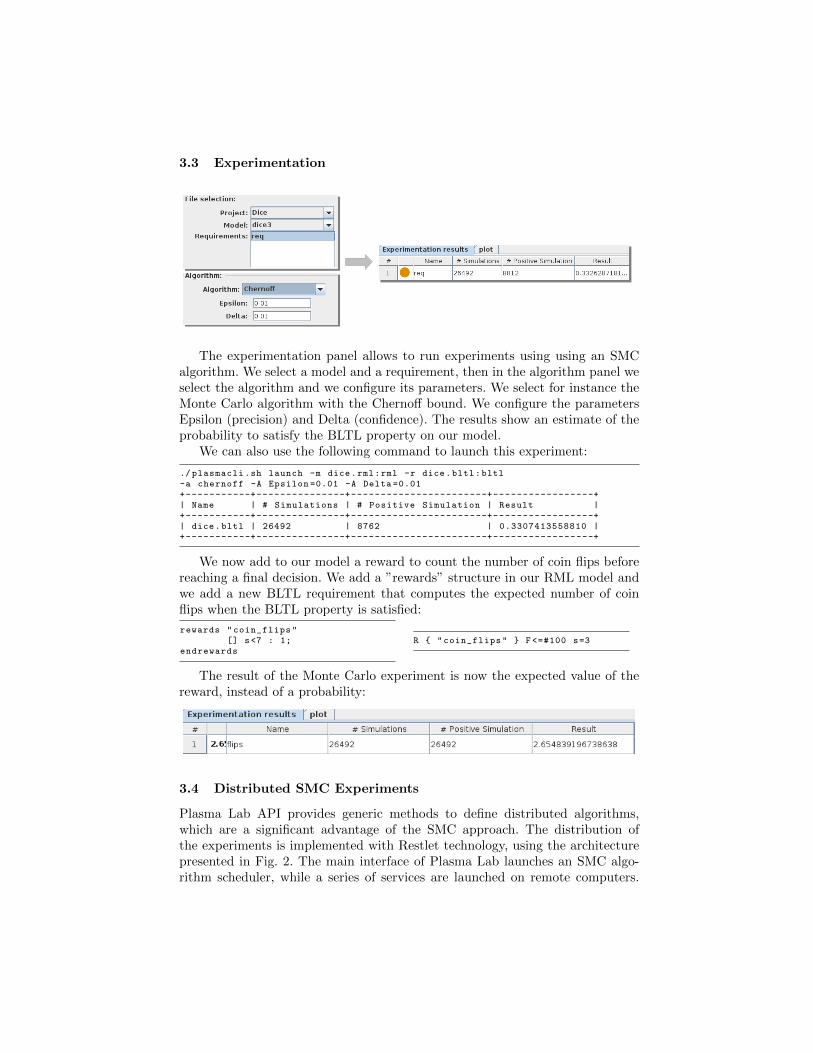
3.3 Experimentation

The experimentation panel allows to run experiments using using an SMCalgorithm. We select a model and a requirement, then in the algorithm panel weselect the algorithm and we configure its parameters. We select for instance theMonte Carlo algorithm with the Chernoff bound. We configure the parametersEpsilon (precision) and Delta (confidence). The results show an estimate of theprobability to satisfy the BLTL property on our model.

We can also use the following command to launch this experiment:

./ plasmacli.sh launch -m dice.rml:rml -r dice.bltl:bltl-a chernoff -A Epsilon =0.01 -A Delta =0.01+-----------+---------------+-----------------------+-----------------+| Name | # Simulations | # Positive Simulation | Result |+-----------+---------------+-----------------------+-----------------+| dice.bltl | 26492 | 8762 | 0.3307413558810 |+-----------+---------------+-----------------------+-----------------+

We now add to our model a reward to count the number of coin flips beforereaching a final decision. We add a ”rewards” structure in our RML model andwe add a new BLTL requirement that computes the expected number of coinflips when the BLTL property is satisfied:

rewards "coin_flips"[] s<7 : 1;

endrewardsR { "coin_flips" } F <=#100 s=3

The result of the Monte Carlo experiment is now the expected value of thereward, instead of a probability:

3.4 Distributed SMC Experiments

Plasma Lab API provides generic methods to define distributed algorithms,which are a significant advantage of the SMC approach. The distribution ofthe experiments is implemented with Restlet technology, using the architecturepresented in Fig. 2. The main interface of Plasma Lab launches an SMC algo-rithm scheduler, while a series of services are launched on remote computers.

Fig. 2: Distributed architecture.Fig. 3: Execution panel.

Each service is loaded with a copy of the model simulator and a copy of theproperty checker. Then, the scheduler sends work orders to the services, viaRestlet. These orders consist in performing a certain number of simulations andchecking them with the checker. When a service has finished its work it sendsthe result back to the scheduler. According to the SMC algorithm, the schedulereither displays the results via the interface or decides that more work is needed.

We can configure the distributed mode in the GUI in the execution panelpresented in Fig. 3. . In local mode the algorithm runs the simulations locally onone or several threads. In distributed mode the algorithm starts a scheduler andwaits for clients to connect. It will then request the clients to perform a numberof simulations configured with the Batch parameter and then it waits for theresults.

3.5 SMC and Nondeterminism

Classical SMC algorithms can only be apply to fully stochastic models, such asMarkov chains. With RML we can design Markov decision processes (MDP) thatinterleave probabilistic transitions with nondeterministic transitions. The choiceand the order of nondeterministic transitions can radically affect the probabilityto satisfy a given property or the expected reward. Since it is useful to evaluatethe upper and lower bounds of these quantities, we are interested in finding theoptimal schedulers that do this.

We reuse our previous model of a 3-valued dice and we construct a MDPwith two dices. We will roll each dice once and we allow to re-roll one dice. Wewould like to estimate the minimum and maximum probabilities that both dicesreturn the same value. We modify our RML model accordingly:

mdp

global r : [0..1] init 0;

module dices : [0..3] init 0;d : [0..3] init 0;

[ ] s=0 -> 0.5 : (s’=1) + 0.5 : (s’=2);[ ] s=1 -> 0.5 : (s ’=3)&(d’=1) + 0.5 : (s ’=3)&(d’=2);[ ] s=2 -> 0.5 : (s ’=3)&(d’=3) + 0.5 : (s’=0);

[ ] s=3 & r=0 -> (s ’=0)&(r’=1);[ ] s=3 & r=0 -> (r’=1);

endmodule

module dice2 = dice[s=s2,d=d2] endmodule

We change the type from dtmc to mdp. Then we add a global variable r thatwill count the number of re-roll (maximum 1). In the dice module, we add twocommands, one that allows to re-roll the dice, and one that decide to stop. Sincethese two commands are enabled at the same condition (s=3 & r=0) the choicebetween the two is nondeterministic. Finally we add a second dice that is a copyof the first module in which the variables s and d are renamed s2 and d2. Theorder in which the two dices will be rolled is also nondeterministic.

Several algorithms of Plasma Lab can be use with nondeterministic models.When using Monte Carlo algorithms, the default behavior is to simulate themodel using a uniform distribution for nondeterministic choices. However theMDP option in the Chernoff algorithm allows to specify the number of schedulersto evaluate. Scheduler are randomly chosen and evaluated by an SMC experimentusing the confidence bound for multiple schedulers [8]. The result displays boththe minimum and the maximum probability.

This simple sampling has the disadvantage of allocating equal budget to allschedulers, regardless of their merit. To maximize the probability of finding anoptimal scheduler with finite budget, Plasma Lab implements “smart sampling”algorithms [3,9], comprising three stages:

1. An initial undirected sampling experiment to approximate the distributionof schedulers and discover the nature of the problem.

2. A targeted sampling experiment to generate a candidate set of schedulerswith high probability of containing an optimal scheduler.

3. Iterative refinement of the candidate set of schedulers, to identify the bestscheduler with specified confidence.

Note that smart hypothesis testing may quit at any stage if an individual sched-uler is found to satisfy the hypothesis with required confidence or if individualschedulers do not satisfy the hypothesis with required confidence but the averageof all schedulers satisfies the hypothesis.

This algorithm has several options, several of them being optional. The nec-essary parameters are Epsilon, Delta, that define the confidence bound, andBudget, that defines a fix number of simulations to perform at each stage. Theother parameters have default values that can be substituted to optimize theperformances of the algorithm:

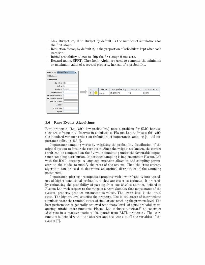
– Max Budget, equal to Budget by default, is the number of simulations forthe first stage.

– Reduction factor, by default 2, is the proportion of schedulers kept after eachiteration.

– Initial probability allows to skip the first stage if not zero.– Reward name, SPRT, Threshold, Alpha are used to compute the minimum

or maximum value of a reward property, instead of a probability.

3.6 Rare Events Algorithms

Rare properties (i.e., with low probability) pose a problem for SMC becausethey are infrequently observes in simulations. Plasma Lab addresses this withthe standard variance reduction techniques of importance sampling [4] and im-portance splitting [5,6,7].

Importance sampling works by weighting the probability distribution of theoriginal system to favour the rare event. Since the weights are known, the correctresult can be computed on the fly while simulating under the favourable impor-tance sampling distribution. Importance sampling is implemented in Plasma Labwith the RML language. A language extension allows to add sampling param-eters to the model to modify the rates of the actions. Then the cross entropyalgorithm can be used to determine an optimal distribution of the samplingparameters.

Importance splitting decomposes a property with low probability into a prod-uct of higher conditional probabilities that are easier to estimate. It proceedsby estimating the probability of passing from one level to another, defined inPlasma Lab with respect to the range of a score function that maps states of thesystem×property product automaton to values. The lowest level is the initialstate. The highest level satisfies the property. The initial states of intermediatesimulations are the terminal states of simulations reaching the previous level. Thebest performance is generally achieved with many levels of equal probability, re-quiring suitable score functions. Plasma Lab includes a “wizard” to constructobservers in a reactive modules-like syntax from BLTL properties. The scorefunction is defined within the observer and has access to all the variables of thesystem [7].

Plasma Lab implements a fixed level algorithm and an adaptive level algo-rithm [6,7]. The fixed level algorithm requires the user to define a monotonicallyincreasing sequence of score values whose last value corresponds to satisfyingthe property. The adaptive algorithm finds optimal levels automatically and re-quires only the maximum score to be specified. Both algorithms estimate theprobability of passing from one level to the next by the proportion of a constantnumber of simulations that reach the upper level from the lower. New simula-tions to replace those that failed to reach the upper level are started from stateschosen uniformly at random from the terminal states of successful simulations.The overall estimate is the product of the estimates of going from one level tothe next.

We consider a simple DTMC model that implements a chain of 100 states,with at each state a probability of 0.9 to pass to the next state, and a prob-ability of 0.1 to exit to a state s=101. We want to estimate the probability toreach the final state s=100. We can use Monte Carlo with the BLTL propertyF<=#100 s=100. However the number of simulations must be very large to ob-serve a significant number of successful traces. Otherwise we can use importancesplitting with an observer that compute a score function: the score is equal tothe last state reached in the trace.

dtmc

module chains : [0..101] init 0;[] s<100 -> 0.90 : (s’=s+1)

+ 0.10 : (s ’=101);endmodule

observer chainObserverscore : double init 0;decided : bool init false;

[] s!=101 & score <s -> (score ’=score +1);[] s>=100 -> (decided ’=true);

endobserver

We compare in Table 5 the Monte Carlo algorithm, with 1’000’000 simula-tions, the fixed levels importance splitting algorithm, with 4 levels and 1’000simulations, and the adaptive importance splitting algorithm with 1’000 simu-lations. Each experiment is performed 10 times and the table shows the averageand the standard deviation of these 10 executions. The results show that the fixedlevels algorithm produces an answer with a similar variance to Monte Carlo ina much faster time. The adaptive algorithm also produces a fast answer, andadditionally improves the variance.

Fig. 4: Plasma Lab parameters forimportance splitting.

Probability Time Std. dev.

Monte Carlo 2.8E-5 7.93s 5.08E-6Fixed levels 2.61E-5 0.58s 5.35E-6Adaptive 2.56E-5 0.2s 1.88E-6

Fig. 5: Comparison between importancesplitting algorithms and Monte Carlo

4 Plugin Development Tutorial

This tutorial explains how to develop a new simulator plugin for Plasma Lab.The sources of this tutorial can be downloaded on our documentation website(http://plasma-lab.gforge.inria.fr/plasma_lab_doc/1.4.0/html/developer/tutorials/index.html).

In Plasma Lab the concepts of simulator and model are mixed together.We could say that a model executes itself. For this reason, a simulator inheritsfrom the AbstractModel class, that in turn inherits from the AbstractData class.The AbstractData class describes an object, model or requirement, editable inthe Plasma Lab GUI edition panel. The AbstractModel class adds simulationmethods.

In this section, we explain some of the implementation needed for a newsimulator plugin. The language executed by our tutorial simulator is a successionof ’+’and ’-’. Starting from 0 it will add or remove one to the single value ofthe state. For instance the model +++-- will produce a trace 0 1 2 3 2 1. Ofcourse this language is only used to illustrate the plugin creation and it has nostochastic property. We begin our simulator with the class declaration:

public class MySimulator extends AbstractModel

4.1 Factory

To load our simulator plugin in Plasma Lab we need a factory class that ex-tends AbstractModelFactory. The factory class implements a new JSPF Plugin.Its plugin nature is declared using the annotation @PluginImplementation beforethe class declaration.

@PluginImplementationpublic class MySimulatorFactory extends AbstractModelFactory

The main purpose of the factory is to instantiate a simulator or a checkerwithout knowing its class. This is done by implementing the createAbstractModelmethods to call the simulator constructor. For instance:

public AbstractModel createAbstractModel(String name , String content) {return new MySimulator(name , content , getId ());

}

The factory also implements methods to identify a plugin by returning thename of the factory as it appears in the GUI menus (getName), a short textualdescription (getDescription), and a unique identifier (getId).

4.2 State and Identifiers

To create our new simulator we first need some companion objects to manipulatevalues and states. Identifiers are a shared objects to identify values (e.g. variables,constants) through different components of Plasma Lab. We create a new classMyId that implements the InterfaceIdentifier interface:

public class MyId implements InterfaceIdentifier {String name;

public MyId(String name) {this.name = name;

}}

In our model we manipulate only two variables, the value and the time. Wecan declare them as static identifiers in the MySimulator class:

protected static final MyId VALUEID = new MyId("X"); // VALUEprotected static final MyId TIMEID = new MyId("#"); // TIME

The state object is used to store the values of the model. It inherits from theInterfaceState interface. Our state object is pretty simple as we store only thetwo variables, time and value.

public class MyState implements InterfaceState {double value , time;

public MyState(double value , double time) {this.value = value;this.time = time;

}

The class MyState additionally implements getters and setters to access andmodify the values of the state, either through an InterfaceIdentifier object orthrough their name. For instance the following method returns the values thestate according to the identifier:

public Double getValueOf(InterfaceIdentifier id) {if(id.equals(MySimulator.VALUEID ))

return value;else if(id.equals(MySimulator.TIMEID ))

return time;else

throw new PlasmaRunException("Unknown identifier: "+id.getName ());}

4.3 Check for errors

The checkForErrors method is called before each experimentation/simulation andwhen modifying the content of the edition panel of the GUI. The purpose of thisfunction is double: to detect any syntax error and to build the model beforerunning it. Our checkForErrors method checks if the sequence contains any othercharacters than ’+’, ’-’. In the eventuality of a syntax error, a PlasmaSyntaxEx-ception is added to the list of errors. Finally we create the initial state that willbe used to initialize each trace.

@Overridepublic boolean checkForErrors () {

// Empty from previous errorserrors.clear ();

// Verify model contentInputStream is = new ByteArrayInputStream(content.getBytes ());

br = new BufferedReader(new InputStreamReader(is));try {

while(br.ready ()){int c = br.read ();if(!(c==’+’||c==’-’))

errors.add(new PlasmaSyntaxException("Not a valid command"));

}} catch (IOException e) {

errors.add(new PlasmaException(e));}initialState = new MyState (0,0);return !errors.isEmpty ();

}

4.4 New path

The newPath method initializes a new trace and returns the first state of thetrace. content is a String inherited from AbstractData that contains the textentered in the edition panel. In our simulator we initialize a stream reader toread content character by character. We also initialize the trace with the initialstate created by the checkForErrors method.

public InterfaceState newPath () {trace = new ArrayList <InterfaceState >();trace.add(initialState );InputStream is = new ByteArrayInputStream(content.getBytes ());br = new BufferedReader(new InputStreamReader(is));return initialState;

}

4.5 Simulate

The simulate method adds a new state to the trace. In our simulator we read thenext character (’+’ or ’-’) and we either add or subtract 1 to the value of the cur-rent state. We also add 1 to the time. Finally we build a new state with the newvalues. If there is no more character to read we throw a PlasmaDeadlockExceptioninstead of adding a new state to the trace.

public InterfaceState simulate () throws PlasmaDeadlockException {try {

if (!br.ready ())throw new PlasmaDeadlockException(getCurrentState (),

getTraceLength ());else {

int c = br.read ();InterfaceState current = getCurrentState ();double currentV = current.getValueOf(VALUEID );double currentT = current.getValueOf(TIMEID );if(c==’+’)

trace.add(new MyState(currentV+1,currentT +1));else if(c==’-’)

trace.add(new MyState(currentV -1,currentT +1));}

} catch (IOException e) {throw new PlasmaSimulationException(e);

}return getCurrentState ();

}

References

1. Biere, A., Heljanko, K., Junttila, T.A., Latvala, T., Schuppan, V.: Linear Encod-ings of Bounded LTL Model Checking. Logical Methods in Computer Science 2(5)(2006)

2. Boyer, B., Corre, K., Legay, A., Sedwards, S.: PLASMA-lab: A Flexible, Dis-tributable Statistical Model Checking Library. In: Proceedings of QEST. LNCS,vol. 8054, pp. 160–164. Springer (2013)

3. D’Argenio, P., Legay, A., Sedwards, S., Traonouez, L.: Smart sampling forlightweight verification of markov decision processes. STTT 17(4), 469–484 (2015)

4. Jegourel, C., Legay, A., Sedwards, S.: Cross-entropy optimisation of importancesampling parameters for statistical model checking. In: Proceedings of CAV. LNCS,vol. 7358, pp. 327–342. Springer (2012)

5. Jegourel, C., Legay, A., Sedwards, S.: Importance Splitting for Statistical ModelChecking Rare Properties. In: Proceedings of CAV. LNCS, vol. 8044, pp. 576–591.Springer (2013)

6. Jegourel, C., Legay, A., Sedwards, S.: An effective heuristic for adaptive importancesplitting in statistical model checking. In: Proceedings of ISoLA (2). LNCS, vol.8803, pp. 143–159. Springer (2014)

7. Jegourel, C., Legay, A., Sedwards, S., Traonouez, L.: Distributed verification ofrare properties using importance splitting observers. ECEASST 72 (2015)

8. Legay, A., Sedwards, S., Traonouez, L.: Scalable verification of markov decision pro-cesses. In: SEFM Collocated Workshops. LNCS, vol. 8938, pp. 350–362. Springer(2014)

9. Legay, A., Sedwards, S., Traonouez, L.: Estimating rewards & rare events in non-deterministic systems. ECEASST 72 (2015)

10. Okamoto, M.: Some inequalities relating to the partial sum of binomial probabili-ties. Annals of the Institute of Statistical Mathematics 10, 29–35 (1959)

11. Wald, A.: Sequential tests of statistical hypotheses. The Annals of MathematicalStatistics 16(2), 117–186 (1945)