Accepted for publication in the Astrophysical Journal

Tatooine’s Future: The Eccentric Response of Kepler’s CircumbinaryPlanets to Common-Envelope Evolution of their Host Stars

Veselin B. Kostov1,6, Keavin Moore2, Daniel Tamayo3,4,5, Ray Jayawardhana2,Stephen A. Rinehart1

veselin.b.kostov@nasa.gov

ABSTRACT

Inspired by the recent Kepler discoveries of circumbinary planets orbiting nineclose binary stars, we explore the fate of the former as the latter evolve off the main se-quence. We combine binary star evolution models with dynamical simulations to studythe orbital evolution of these planets as their hosts undergo common-envelope stages,losing in the process a tremendous amount of mass on dynamical timescales. Fiveof the systems experience at least one Roche-lobe overflow and common-envelopestages (Kepler-1647 experiences three), and the binary stars either shrink to veryshort orbits or coalesce; two systems trigger a double-degenerate supernova explo-sion. Kepler’s circumbinary planets predominantly remain gravitationally bound atthe end of the common-envelope phase, migrate to larger orbits, and may gain sig-nificant eccentricity; their orbital expansion can be more than an order of magnitudeand can occur over the course of a single planetary orbit. The orbits these planetscan reach are qualitatively consistent with those of the currently known post-common-envelope, eclipse-time variations circumbinary candidates. Our results also show thatcircumbinary planets can experience both modes of orbital expansion (adiabatic and

1NASA Goddard Space Flight Center, Mail Code 665, Greenbelt, MD, 20771

2Faculty of Science, York University, 4700 Keele Street, Toronto, ON M3J1P3, Canada

3Department of Physical & Environmental Sciences, University of Toronto at Scarborough, Toronto, Ontario M1C1A4, Canada

4Canadian Institute for Theoretical Astrophysics, 60 St. George St, University of Toronto, Toronto, Ontario M5S3H8, Canada

5CPS Postdoctoral Fellow

6NASA Postdoctoral Fellow

arX

iv:1

610.

0343

6v1

[as

tro-

ph.E

P] 1

1 O

ct 2

016

– 2 –

non-adiabatic) if their host binaries undergo more than one common-envelope stage;multiplanet circumbinary systems like Kepler-47 can experience both modes duringthe same common-envelope stage. Additionally, unlike Mercury orbiting the Sun, acircumbinary planet with the same semi-major axis can survive the common envelopeevolution of a close binary star with a total mass of 1 M�.

Subject headings: binaries: eclipsing, close – planetary systems – stars: individual(Kepler-34, -35, -38, -47, -64, -1647, NN Ser, HU Aqu, V471 Tau) – techniques:photometric – methods: numerical

1. Introduction

“Everything is in motion”, Plato quotes Heraclitus (Cratylus, Paragraph 402, section a, line 8),“and nothing remains still.”. Despite the overwhelming timescales, from a human perspective, thenatural life-cycle of stars is a prime example of change on the cosmic stage. Following the lawsof stellar astrophysics, over millions to billions of years, stars and stellar systems form, evolve,and ultimately die (e.g. Kippenhahn & Wiegert 1990 and references therein). And so do planetarysystems, with their fate linked intimately to that of their stellar hosts.

The fate of planets orbiting single stars has been studied extensively, indicating that planetscan survive their star’s evolution if they avoid engulfment and/or evaporation during the Red GiantBranch (RGB) and the Asymptotic Giant Branch (AGB) stages (e.g. Livio & Soker 1984; Rasio &Livio 1996; Duncan & Lissauer 1998; Villaver & Livio 2007). There is also accumulating evidenceof planetary or asteroidal debris surrounding white dwarfs and polluting their atmospheres (seerecent reviews by Farihi 2016 and Veras 2016). A planet’s survival depends both on the initialorbital separation, and on its mass. For example, even a planet as massive as 15 MJup aroundan 1M� MS star can be destroyed inside the stellar envelope during the AGB phase (Villaver &Livio 2007). An unpleasant prospect for the future of our own planet is that it might not survivethe evolving Sun (e.g. Schroder&Connon Smith 2008). Despite the complications, theoreticalconsiderations indicate that planets can indeed survive the evolution of single stars (Villaver &Livio 2007), and there is mounting observational evidence supporting this (e.g. Reffert et al. 2015;Wittenmyer et al. 2016, and references therein1).

Single stars, however, do not have monopoly over planetary systems. Nearly half of Solar-type stars are members of binary and higher order stellar systems (Raghavan et al. 2010), and an

1Also see https://www.lsw.uni-heidelberg.de/users/sreffert/giantplanets.html for a list of known systems.

– 3 –

increasing number of planets have been discovered in such systems. While the presence of a dis-tant stellar companion will have little effect on a planet around one (evolving) member of a widebinary stellar system (& 100 AU), a planet orbiting around both members of a close binary system(separation ∼ 10 AU or less) will experience qualitatively and quantitatively different stellar evo-lution. Namely, where a single star loses mass and expands on timescales of millions to billionsof years (Veras 2016) while on the main sequence (MS), the RGB and the AGB – its planets reactaccordingly – close binary stars can experience events of dramatic mass loss, orbital shrinkageon timescales of years, and common envelope (CE hereafter, see Appendix for abbreviations andparameters) stages where the two stars share (and quickly expel) a common atmosphere (Paczyn-ski 1976; Hilditch 2001). During the in-spiralling CE phase, the two stars can strongly interactwith each other by transferring mass, smoothly coalesce or violently collide, or even explodes asa supernova (SN). Both the amount of energy released during this stage and the timescale of therelease are staggering – a close binary star can lose an entire solar mass over the course of just afew months (e.g. Rasio & Livio 1996; Livio & Soker 1984; Ivanova et al. 2013; Passy et al. 2012;Ricker & Taam 2008, 2012; Nandez et al. 2014, but also see Sandquist et al. 1998 and De Marcoet al. 2003 for longer timescales); in the extreme case of a SN, the binary will be completely dis-rupted. Overall, the evolution of close binary stars is much richer compared to single stars, as theseparation, eccentricity and metallicity of the binary add additional complications to an alreadycomplex astrophysical process. Interestingly, to date there are 9 close main-sequence binary sys-tems harboring confirmed circumbinary planets (hereafter CBPs, Doyle et al. 2011; Welsh et al.2012, 2015; Orosz et al. 2012a,b; Kostov et al. 2013, 2014; Schwamb et al. 2013. It is reasonableto assume that the reaction of these planets to the violent CE phase of their host binary stars willbe no less dramatic.

Previous studies of the dynamical response of planets in evolving multiple stellar systemshave focused on post-CE (hereafter PCE) CBP candidates (e.g. Volschow, Banerjee, & Hessman2013; Portegies Zwart 2013; Mustill et al. 2013), of circumprimary planets in evolving wide binarysystems (Kratter & Perets 2012), and of the survival prospects of CBP planets (Veras et al. 2011,2012). In particular, Portegies Zwart (2013) and Mustill et al. (2013) start with the final outcomeof close binary evolution – PCE systems with candidate CBP companions (HU Aqu and NN Serrespectively) – and reconstruct the initial configuration of their progenitors.

Inspired by recent discoveries of planets in multiple stellar systems, here we tackle the reverseproblem – we start with the 9 confirmed CBP Kepler systems with known initial binary configura-tions (using data from NASA’s Kepler mission), and study their dynamical response as their stellarhosts evolve. We combine established, publicly-available binary stellar evolution code (BSE; Hur-ley, Tout, & Pols 2002) with direct N-body integrations (using REBOUND, Rein & Liu 2012)allowing for stellar mass loss and orbital shrinkage on dynamical timescales. For simplicity, herewe focus explicitly on dynamical interactions only (e.g. no stellar tides), and assume that the CBPs

– 4 –

do not interact with the ejected stellar material. We expand on the latter limitation in Section 5.1.

We note that Mustill et al. (2013) assume adiabatic mass-loss regime (Hadjidemetriou 1963)during the CE stage for the evolution of NN Ser. In this case, the orbital period of the CBP ismuch shorter than the CE mass-loss timescale (hereafter TCE), and the planet’s orbit expands atconstant eccentricity2. Volschow, Banerjee, & Hessman (2013) study the two analytic extremes ofmass-loss events for the case of NN Ser – the adiabatic regime, and the instantaneous regime whereTCE is much shorter than the orbital period of the planets3. The Kepler CBP systems, however,occupy a unique parameter space where the planets’ periods are comparable to the TCE used byPortegies Zwart (2013) and suggested by Ricker & Taam (2008, 2012) for binary systems similarto Kepler CBP hosts. Thus the adiabatic approximation may not be an adequate assumption whentreating the CE phases of these systems. Specifically, the CE phase can occur on timescales as shortas one year (Paczynski 1976; Passy et al. 2012), and during this year a binary can expel ∼ 2M�worth of mass (Ricker & Taam 2008, 2012; Iaconi et al. 2016). Interestingly, such timescales arewell within a single orbit of CBPs like Kepler-1647 with PCBP= 3 yrs (Kostov et al. 2016). Such adramatic restructuring will have a profound impact on the dynamics of the system – for example, aCBP can achieve very high eccentricity – and may even result in the ejection of the planet. Similarto Portegies Zwart (2013), here we tackle such complications by directly integrating the equationsof motions during the CE phases for each Kepler CBP system.

The transition from adiabatic to non-adiabatic regime can be characterized through a mass-loss index ψ. For a planet orbiting a single star Veras et al. (2012) define:

Ψ≡ αM

nµ= (2π)−1

(αM

1M� yr−1

)( ap,0

1 AU

) 32(

µ1 M�

)− 32

(1)

where αM is the mass-loss rate, ap,0 is the initial semi-major axis of the planet, and µ = Mstar +Mp

is the total mass of the system4. If Ψ� 1 then the evolution of the planet’s orbit is in the adiabaticregime and its semi-major axis grows at constant eccentricity.

Alternatively, if Ψ� 1 then the planet sees an ‘instantaneous’ mass loss and its orbital evolu-tion is in a ‘runaway’ regime. In this scenario, the fate of the planet depends on the ratio betweenthe final and initial mass of the system, i.e. β = µfinal/µinit, and on the orbital phase of the planet

2In line with thermodynamics nomenclature, this is an isoeccentric process.

3We note that both the total amount of mass lost, and the rate at which it is lost will affect the evolution of a CBP’sorbit during a CE phase.

4Throughout this paper we use subscripts “bin”, and “p” or “CBP” to denote the binary star and the CBP, and “M1”and “M2” to denote the mass of the primary and the secondary star respectively.

– 5 –

at the onset of the mass-loss event. For example, if a highly-eccentric planet is at pericenter at thebeginning of the CE stage it becomes unbound. Overall, ejection occurs when the system losessufficient mass by the end of the mass loss event. To first order, the critical mass ratio for ejectionβeject is given by Eqn. 39 of Veras et al. (2011), which we reproduce here for completeness:

βeject ≡ 0.5(1+ ep,0) (2)

where ep,0 is the eccentricity of the planet at the beginning of the mass-loss event. A planet ona circular orbit or at pericenter is ejected from the system if β < βeject

5. A planet at apocenterremains bound even in the runaway regime, its orbit expands to arunaway,apocenter and circularizes,or reaches an eccentricity of e(post−circ). If a planet remains bound in the runaway regime, it’ssemi-major axis is given by Eqn. 43 and 44 of Veras et al. (2011):

arunaway ≡ap,0(1∓ ep,0)

2−β(1± ep,0)(3)

where the signs represent initial pericenter/apocenter respectively.

According to the above prescription, the dynamical evolution of a CBP’s orbit for Ψ∼ 0.1−1lies between these two regimes. For both Ψ ∼ 1 and Ψ� 1, the evolution is not adiabatic andeCBP can vary (increase or decrease) as aCBP varies. Thus the planet may become unbound onlyif Ψ & 1, with the caveat that the transition is not clear-cut and the Ψ ∼ 0.1− 1 regime is morecomplex (Portegies Zwart 2013; Veras et al. 2011, 2012; Veras 2016). As we show below, the factthat the central object in a CBP system is itself a binary instead of a single star adds yet anotherlayer of complication to these theoretical considerations.

Based on Eqn. 1, and assuming CE timescale of TCE ∼ 103 yrs, we would a priori expect thatall Kepler CBPs remain bound to their hosts during their primary stars’ CE stage (e.g., see Fig. 3,Veras et al. 2012). However, for the rapid CE timescale of TCE ∼ 1 yr suggested by recent results(e.g. Ricker & Taam 2008, 2012), some of the Kepler CBP systems are within a factor of 5-10 ofthe transition to non-adiabatic regime during the primary or secondary CE (i.e. Ψ ∼ 0.1− 0.2),and within a factor of 2 of the transition during their respective secondary CE stage (i.e. Ψ∼ 0.5).We might therefore expect significant variations in the respective CBPs’ orbital eccentricities, aswell as deviations from the final semi-major axes expected from adiabatic mass loss.

As the transition between adiabatic and non-adiabatic regimes is difficult to study analyti-cally, here we examine the dynamical evolution of all Kepler CBP systems numerically, using the

5Also see Eqn. 48 from Veras et al. (2011) for a comprehensive treatment.

– 6 –

adaptive-timestep, high-order integrator IAS15 (Rein & Spiegel 2015), which is available as partof the modular and open-source REBOUND package (Rein & Liu 2012). REBOUND is writtenin C99 and comes with an extensive Python interface.

This paper is organized as follows. In Section 2 we describe the algorithm we use for theevolution of the Kepler CBP hosts. Section 3 details our implementation of an N-body code inexploring the dynamical reaction of said CBPs to the respective CE stages. We present the resultsfor each system in Section 4, and discuss our results and draw conclusions in Section 5.

2. Binary Star Evolution

The evolution of a gravitationally-bound system of two stars depends primarily on its initialconfiguration. If the binary is wide enough the stars will evolve in isolation, according to theprescription of single-star evolution theory. Alternatively, if the initial separation is sufficientlysmall then the stars will influence each other’s evolution. The evolution of such systems, describedas close (or interacting) binary stars (Hilditch 2001), is more complex and includes a number ofadditional processes such as tidal interactions, mass transfer, etc. The 9 Kepler CBP-harboringbinary systems fall in the latter category, and we use the established, open-source Binary StarEvolution code (Hurley, Tout, & Pols 2002) to study their evolution. Briefly, the code works asfollows.

While the binary is in a detached state, the code evolves each star individually using a singlestar evolutionary code (Hurley, Pols, & Tout 2000) which includes tidal and braking mechanisms,and wind accretion. When the stars begin to interact, BSE uses a suite of binary-specific featuressuch as mass transfer and accretion, common-envelope evolution, collisions and mergers, and an-gular momentum loss mechanisms. The evolution algorithm allows the specific processes to beturned on and off, or even modified based on custom requirements. By default, all stars are as-sumed to be initially on the zero-age main sequence (ZAMS), but any possible evolutionary state,such as corotation with the orbit, can be the starting point of the simulation. BSE uses an evolutiontime-step small enough to prevent the stellar mass and radius from changing too much (not morethan 1% in mass and 10% in radius), which allows identifying the time when, and if, a star firstfills its Roche lobe.

At the onset of Roche lobe overflow (RLOF), the two stars either come into contact andcoalesce, or initiate a common envelope (CE) stage. CE evolution is a complex mechanism thattypically occurs when an evolved, giant star transfers mass to a main sequence (MS hereafter) star

– 7 –

on a dynamical timescale6. When the giant star overfills the Roche lobe of both stars, its core andthe MS star share a single envelope. This envelope rotates slower than the orbiting “cores” withindue to expansion, and the resulting friction causes in-spiral and energy transfer to the envelope,described by an efficiency parameter αCE . The outcome of this phase is either ejection of theenvelope (assumed to be isotropic) if neither core fills its Roche lobe, leaving a close white dwarf-MS pair (assumed to be in corotation with the orbit), or coalescence of the cores. A challengingprocess to study numerically, BSE recognizes the CE phase – beginning with RLOF – and forcesthe system through it on an instantaneous timescale, allowing the evolution to continue accordingto the appropriate PCE parameters. The code resolves the outcome of the CE phase based on theinitial binding energy of the envelope and on the initial orbital energy of the two cores7.

On input BSE requires a number of parameters. Namely, the CE efficiency parameter αCE (inthe range of 0.5− 10), the masses and stellar types of both the primary and secondary stars (inthe range of 0.1− 100M�), the binary orbital period (in days), eccentricity (0.0− 1.0), and themaximum time for the evolution (here we choose 15 Gyr, roughly the age of the Universe, unless aparticular Kepler CBP system stops evolving – or the stars coalesce – much sooner, at which pointwe stop the simulations), and the metallicity (0.0001−0.03) of the system. The code also checkswhether tidal evolution is included, i.e. “on” (hereafter TCP for tidal circularization path) or “off”(NTCP for no tidal circularization path). Given the still-uncertain mechanism of the CE stage, theparameters describing the efficiency of envelope ejection and the treatment of tidal decay – andtheir associated uncertainties – are likely the dominant source of error in our BSE results.

Depending on αCE , a binary system may exit a CE stage as a merged star, as a very tight PCEbinary star, or may even trigger a Supernova explosion. For example, a higher αCE accounts forenergy sources other than orbital energy, and the system then requires less energy to dissipate theenvelope. The BSE code also allows an alternate CE model to be used, the de Kool CE evolutionmodel (de Kool 1990), which first introduced the CE evolution binding energy factor λ.

Likewise, tides are integral to the evolution of close binary stars. The strength of tidal dissi-pation will affect the orbital separation and eccentricity when mass transfer begins, and hence thefuture evolution under RLOF or a CE stage. BSE achieves orbital circularization mainly throughtides, but also by accounting for more mass accretion at pericenter than apocenter of an eccentricorbit. Another effect is the exchange of orbital angular momentum with the component spins dueto tidal synchronization, thus causing the evolution to proceed in a similar way to closer binarysystems if tides were ignored. In addition, primary spin-orbit corotation can be forced within the

6A collision between a dense core and a star can also trigger a CE phase.

7BSE also accounts for collisions which do not proceed through CE evolution, and for the possibility of core-sinking depending on the stellar types (which may lead to rejuvenation).

– 8 –

code to avoid unstable RLOF, which gives two possible outcomes for each system. To accountfor the effect of tides on binary evolution, we use both the tides “on” (i.e. TCP) or “off” (i.e.NTCP) options in BSE. As a result, the binary starts the first RLOF at either ebin,RLOF = 0 andabin,RLOF < abin,0 (for TCP), or at ebin,RLOF = ebin,0 and abin,RLOF = abin,0 (for NTCP).

Additionally, while the binary periods of the Kepler CBP systems are known to very highprecision, their stellar masses and metallicities have non-negligible uncertainties8. For example,the primary masses for Kepler-38 and -64 have 1σ errors of 0.05 MSun and 0.1 MSun respectively,and the 1σ errors on the metallicities of half of the systems are as large as, or even larger than themeasured values. To better characterize the impact of these uncertainties on the evolution of theKepler CBP systems, we obtain BSE results for both the best-fit mass and metallicity values andalso for their corresponding 3σ range9.

The entire parameter space we explored, shown in Table 1, includes a range of CE parametersas well and consists of 22680 BSE simulations. Our default configurations are denoted in boldfacein the table; for the rest of the input parameters we use the default values from model A of Hurley,Tout, & Pols (2002), described as the most favorable and effective. Model A uses all defaultwind-related parameters, and a Reimers mass-loss coefficient of η = 0.5.

As BSE evolves the stars, their types change, and each type is checked throughout the code toensure the correct evolutionary tracks are used for both the individual stars as well as the systemas a whole. These numerical values, as well as what they represent, are listed in Table 2. At eachsignificant event, e.g. at the beginning and end of the RLOF, and of the CE phase, when the starscoalesce or collide, the code also produces a “type” label. These labels, along with their meaning,are shown in Table 3.

An example of the BSE output for Kepler-38, αCE = 0.5, NTCP and TCP is shown in Table 4.The BSE results for all Kepler systems can be found in an online supplement.

In the following section we describe how we use the initial and BSE-generated final binarymasses and orbital separations for each Kepler CBP system to explore the dynamical response ofthe planets during the respective CE stages.

8Interestingly, their metallicities are typically sub-Solar.

9The BSE upper limit of Z = 0.03 restricts some systems with greater Z, such as Kepler-64, to this extreme.

– 9 –

3. Dynamical Simulations

While the concept of CE evolution for binary stars has been proposed 40 years ago (Paczynski1976), detailed understanding of this important stage is a challenging task that requires computationally-intensive hydrodynamical calculations. The outcome of this complex phase has been studied bothnumerically and analytically (see Table 1 of Iaconi et al. 2016 for a list of references). For ex-ample, hydrodynamical simulations by Ricker & Taam (2012) for a 1.05M�+0.36M� binary starwith an initial orbital period of 44-days (similar to Kepler CBP hosts) show that in the later stagesof the CE the system losses mass at a rate of 2 M� yr−1, the binary orbital separation decreasesby a factor of 7 after ∼ 56 days, and ∼ 90% of the outflow is contained within 30 degrees of thebinary’s orbital plane.

To numerically account for the dynamical impact on Kepler CBPs from such drastic orbitalreconfigurations and tremendous, short-timescale mass-loss phases, we use REBOUNDx – a li-brary for incorporating additional effects beyond point-mass gravity in REBOUND simulations(https://github.com/dtamayo/reboundx). In particular, we shrink the binary orbits with theREBOUNDx modify orbits forces routine which adds to the equations of motion a simple dragforce opposite particles’ velocity vectors (Papaloizou & Larwood 2000). When orbit-averaged overa Keplerian orbit, this approach results in an exponential damping of the semimajor axis where thee-folding timescale is set through the particle parameter τa. Hydrodynamical simulations by Passyet al. (2012) and Iaconi et al. (2016) exhibit similar orbital decay during the CE stage (e.g. see theirrespective Figures 5 and 14), validating our approach.

Given the complexities and uncertainties of the mass-loss mechanism during the CE phases,we adopt a simple analytical parametrization similar to the method of Portegies Zwart (2013)who tackled the problem by using a constant mass-loss rate. Here we choose to instead use thesame functional forms for the CE-driven changes in Mstar as we do for abin (utilizing the RE-BOUNDx modify mass routine), i.e. an exponential mass-loss for particles on their assigned e-folding timescales τM. Namely, for a given CE stage where one of the stars transitions from aninitial mass M0 to a final mass M f (both provided by BSE), the mass loss occurs over a timeTCE = (M f −M0)/αM . We note that an exponential mass loss has been explored by Adams, An-derson & Bloch (2013) and Adams & Bloch (2013) as well, but for the case of single-star systems.

To ensure a smooth mass evolution (and avoid possible numerical artifacts) that asymptotes atM f , we linearly evolved REBOUNDx’s exponential mass-loss rate so that it vanished at time TCE .In particular, in terms of the e-folding timescale τM,

M =−MτM

,τM =τM,0

(1− t/TCE )(4)

– 10 –

This differential equation can be solved analytically, yielding

M(t) = M f

(M0

M f

)(1−t/TCE )2

(5)

as long as τM,0 in Eq. 4 is chosen as

τM,0 =TCE

2ln(M0M f

), (6)

As the star’s mass decreases from M0 to M f during the respective CE stage, the binary orbitmust shrink from abin,0 to abin,PCE (as provided by BSE) as well – and both must occur over a timeTCE . We apply the same prescription for evolving abin as that for the mass-loss (i.e. Eqn. 4-6 withτa instead of τM) but caution that while this would evolve abin from abin,0 to abin,PCE in isolation, themass-loss is simultaneously increasing abin . To correct for this, and achieve the desired abin,PCE

we manually adjust the corresponding τa,0 parameter.

While tides are not directly accounted for in our dynamical simulations as the particles in-volved are treated as point masses, we capture their effects in a simple parametrized way. Specif-ically, we impose the same exponential decay to the evolution of ebin as we do for the binary’ssemi-major axis shrinking and stellar mass-loss (i.e. Eqn. 4-6 but with τe). As a result ebin under-goes dampened oscillations during the CE phase at the end of which it settles within a few percentof zero – as required by BSE.

As mentioned in the previous section, while the BSE code yields initial and final values forthe stellar masses and abin at the beginning and end of the CE phases, it does not resolve theextremely rapid mass-loss phase. We bridge this gap by exploring two regimes of mass-loss,namely α1 = 1.0 M�/yr and α0.1 = 0.1 M�/yr, denoted by their respective subscripts. The formeris based on the results of Ricker & Taam (2008, 2012) and Portegies Zwart (2013) for systemssimilar to the Kepler CBP hosts. Values of α0.1 (and smaller) typically guarantee that the orbitalevolution of these CBPs is in the adiabatic regime (see Eq. 1).

To test the applicability of our numerical simulations to the stated problem, we examine theevolution of a mock Kepler-38-like system where the binary is replaced with a single star of thesame total initial and final mass according to the BSE prescription for Kepler-38 (see Table 4),and using the same initial orbit of the planet. Here we test two mass-loss regimes – runaway(for αM = 100.0 M�/yr) and adiabatic (for αM = 0.1 M�/yr ≡ α0.1). The results are shown inFigure 1, where the three panels represent (from upper to lower respectively) the evolution ofthe stellar mass, of the planet’s semi-major axis and of the planet’s eccentricity as a function oftime (such that mass loss starts at t = 0 and ends at t = Tmass−loss). According to the analyticprescription, the planet should remain bound even in the runaway mass-loss regime as the mass

– 11 –

lost is smaller than the critical mass limit for ejection – indicated by the dotted line in the upperpanel of the figure10. The horizontal dashed lines in the middle and upper panels represent thetheoretical adiabatic (green) and runaway (red) approximations. As seen from these two panels,the numerical simulations are fully consistent with the theoretical approximations, demonstratingthe validity and applicability of our simulations.

In order to interpret the results from numerical integrations, it is useful to define a criticalmass loss rate, αcrit , corresponding to Ψ = 1 (see Eq. 1). CBPs in systems with αM� αcrit willexperience ‘instantaneous’ mass loss, while the orbits of those in systems with αM� αcrit shouldevolve adiabatically. A CBP in a system where αM becomes comparable to or larger than αcrit atany point during the binary evolution risks becoming unbound. Secondary CE stages will have twodifferent αcrit values as the respective CBP will have two different values for aCBP and eCBP (butthe same µ) at the end of the preceding CE stages (see Eq. 1) – one for α1, and another for α0.1.We denote these critical values as αcrit (α1) and αcrit (α0.1). In the subsections below, for eachCBP Kepler system we compare αcrit to α1 and α0.1, for each CE phase. Where the adopted α1

is within a factor of 10 of the respective αcrit we pay special attention to the CBP orbit, and testits evolution for 0.1α1, 0.2α1, and 0.5α1 as well. Unless indicated otherwise, the final fate of theCBP for these cases is similar to the case for α1.

The description of a three body system containing an evolving binary star is inherently mul-tidimensional, and minor changes in one parameter can cascade into major changes in the rest.In addition to the importance of αCE, tides and αM, another key issue – as shown in the nextsection – is the phase offset between the binary star and the CBP at the onset of the CE phase,∆θ0 ≡ θCBP,0−θbin,0−ωbin (i.e. the difference between their true anomalies, taking into accountthe binary’s argument of the pericenter).

Thus for each system we test four initial binary phases corresponding to the binary orbit turn-ing points, i.e. Eastern and Western Elongations (EE and WE), Superior and Inferior Conjunctions(SC and IC) and 50 initial CBP phases (between 0 and 1, with a step of 0.02) for a total of 200initial conditions. We explore each of these initial conditions for αCE = (0.5,1.0,3.0,5.0,10.0),for TCP/NTCP, and for α1 and α0.1.

Finally, we note that the post-CE semi-major axis of a CBP (aCBP,PCE) that was initially onan eccentric orbit (i.e. eCBP,0 > 0) depends on its orbital phase at the onset of the CE stage. Forthose Kepler systems that undergo a secondary CE phase with mass-loss, we start the respectiveintegrations at the modes of aCBP,PCE and eCBP,PCE from the preceding CE stage.

10For the planet to be ejected, the final stellar mass must be smaller than M1(runaway,eject).

– 12 –

Fig. 1.— Evolution of, from top to bottom, the stellar mass, the CBP semi-major axis, and ec-centricity for a Kepler-38-like system, where the binary is replaced with a single star which losesmass according to the αCE = 0.5 BSE simulation (for the primary CE phase) for two mass-lossregimes – runaway (red) and adiabatic (green). Here Tmass−loss is the same as the correspondingTCE for Kepler-38, αCE = 0.5. The black dotted line in the upper panel represents the critical masslost which would result in the ejection of the planet. The dashed lines in the middle and lowerpanels indicate the runaway (red) and adiabatic (green) approximations. The numerical evolutionof the planet’s semi-major axis and eccentricity is fully consistent with the theoretical expectation,validating the applicability of our simulations.

– 13 –

4. Results

Here we describe the results of our simulations for those Kepler CBP systems that experienceat least one CE phase. Unless specified otherwise, the evolution of each system is for the defaultCE parameters listed in Table 1. The initial orbital parameters for each system are listed in Table5. We note that our N-body integrations only cover the common envelope phases.

Below we outline the major binary evolution stages (as produced by BSE), along with thedynamical responses of the CBPs; the main results are presented in Tables 6, 7, 8, 9, and 10. Allreported times are in Gyr since ZAMS. For simplicity, we assume that the current Kepler CBPsystems are at ZAMS and that all CBP start on initially circular, coplanar orbits.

Overall, five of the nine Kepler CBP systems experience at least one CE phase for their defaultmetallicities (see Table 1) over the duration of the BSE simulations (15 Gyr): Kepler-34, -38, -47,-64, and -1647. Kepler-35 experiences a CE for Z−1σZ, and Kepler-453 for Z−2σZ.

4.1. Kepler-34

The binary consists of 1.05M�+ 1.02M� stars on a highly-eccentric (ebin,0 = 0.52), 28-dayorbit which changes little in the first ∼ 9 Gyr. The CBP has an initial orbit of 1.09 AU.

The primary star fills its Roche lobe at ∼ 9.6 Gyr, the binary enters a CE stage and triggers adouble-degenerate Supernova event, disrupting the system.

4.2. Kepler-38

The binary consists of 0.95M�+ 0.25M� stars on a slightly-eccentric (ebin,0 = 0.1), 19-dayorbit which changes little in the first ∼ 13 Gyr. The CBP has an initial orbit of 0.46 AU. The mainevolution stages of the binary star and their effect on the CBP are as follows.

4.2.1. The Binary

The primary star fills its Roche lobe at t ∼ 13.7 Gyr and the binary enters a primary CE stage.During this stage Ψ(α1)≈ 0.04 and αcrit ≈ 26 M�/yr – much larger than α1and α0.1. As a resultof the CE, the binary merges as a First Giant Branch star and loses ∼ 25− 40% of its mass forαCE = 0.5; here β > βeject (see Eqn. 3), and the planet should remain bound in a runaway regime(i.e. Ψ� 1) even at pericenter (see Eqn. 37-44, Veras et al. (2011)). The system continues to

– 14 –

slowly lose mass by the end of the BSE simulations (15 Gyr), thus aCBP,PCE adiabatically expandsby up to a factor of 2.

For αCE = 1.0,3.0,5.0,10.0 the binary orbit shrinks by a factor of 4− 30 and its mass de-creases by ∼ 60%; here β < βeject, i.e. planet should be ejected in a runaway regime. For αCE =1 and TCP the system experiences a secondary RLOF at t ∼ 13.74 Gyr and coalesces into a FirstGiant Branch star without mass loss (thus no changes in aCBP,PCE or eCBP,PCE ). The binary doesnot lose mass additional mass by the end of the BSE simulations.

Overall, by 15 Gyr the binary evolves into either a merged Helium or Carbon/Oxygen WhiteDwarf (HeWD, COWD) or a very close HeWD-MS star binary.

The orbital reconfiguration of the binary system during the primary CE stage is shown on theleft panels of Figure 2 for αCE = 0.5 (upper panels) and αCE = 1.0,3.0,5.0,10.0 (lower panels).The observer is looking along the y-axis, from below the figure. The maximum (red dashed; binaryinitially at Eastern Elongation (EE), CBP initially at phase 0.73) and minimum (red solid; binaryat Easter Elongation (EE), CBP at phase 0.08) orbital expansion of the CBP is shown on the rightpanels of the figure for α1(red), as well as the maximum expansion for α0.1(green solid). To testthe dynamical stability of the CBP at maximum expansion (dashed red), we integrated the systemfor a thousand planetary orbits. The orbit precesses, but does not exhibit chaotic behavior for theduration of the integration. We leave examination of the long-term behavior and stability of thesystem for future work.

4.2.2. The CBP

On Fig. 3 we show the αCE = 0.5 CE evolution of M1, abin (blue, upper panel), and ofaCBP (middle panels) and eCBP (lower panel) for α1(red) and α0.1(green) respectively; on Fig. 4we show the corresponding evolution for αCE = 1/3/5/10. Unlike the case of a planet orbitinga single star, where the evolution of the planet’s orbit follows a single path for each αM (seeFig. 1), the dynamical response of a CBP to a binary undergoing a CE stage depends on theinitial configuration of the system, i.e. the phase difference ∆θ0 ≡ θCBP,0−θbin,0−ωbin, whereθCBP,0,θbin,0 are the initial true anomaly of the CBP and the binary respectively, and ωbin is thebinary’s argument of pericenter. This is reminiscent of the importance of the initial true anomalyof a planet orbiting a single star on an eccentric orbit (see Veras et al. (2011)). The dependenceis shown in the second panel of Fig. 3, where each curve represents the evolution of aCBP for∆θ0 varying between 0 and 1 (for clarity, the curves here represent every tenth phase where in thesimulations the phase difference varies with a step of 0.02).

Since our simulations encompass a discrete set of initial conditions for αCE , tides (NTCP

– 15 –

Fig. 2.— Orbital reconfiguration of the Kepler-38 system during the Primary CE stage. The binaryorbits are shown on the left panels (blue for the primary star, magenta for the secondary) and theCBP orbits – on the right (green for α0.1, red for α1, where dashed red corresponds to the largestand the solid red to the smallest achieved orbit). The binary merges for αCE = 0.5. The squaresymbols indicate the initial positions of the two stars and the planet; the circle symbols in the leftpanels indicate the final positions of the primary (blue) and secondary (black) star. The right panelsshow the evolution of aCBP from different initial conditions as indicated by the respective squares.

– 16 –

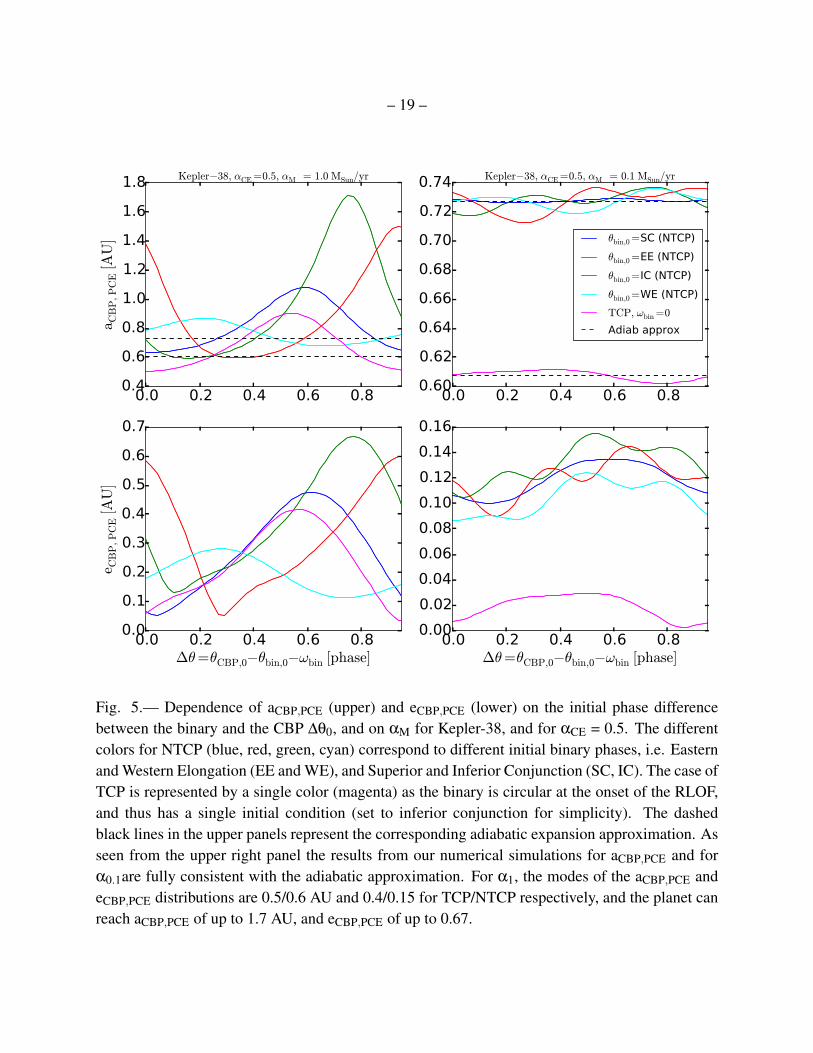
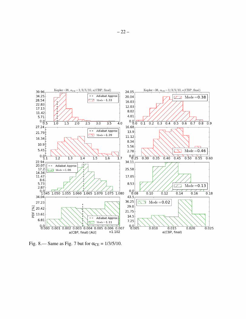
or TCP for minimum to maximum strength respectively), and ∆θ0, the true evolution of aCBP andeCBP would be continuous. We represent this by the hatched regions on the lower panels of Fig.3 and 4, where the different hatches correspond to TCP or NTCP. For clarity, we show individualaCBP evolutionary tracks only in Fig. 3; these are replaced with hatched regions in all subsequentfigures. We note that the distribution of aCBP,PCE and eCBP,PCE (i.e. aCBP and eCBP at the end of theCE phase) is neither uniform nor necessarily normal, as seen from the second panel on Fig. 3, butinstead depends on ∆θ0. This dependence is demonstrated on Fig. 5 for αCE = 0.5 and on Fig. 6for αCE = 1/3/5/10, and the corresponding probability distribution functions (PDFs) are shown inFig. 7 and 8. The PDFs can have a prominent peak with a long one-sided tail (e.g. upper left panelon the first figure), or be double-peaked with the peaks near the edges (e.g. lower left panel on thefirst figure); this is a natural consequence of the vaguely sinusoidal dependencies seen in Figures 5and 6. Given the prominent diversity of the PDFs, the distributions are better represented by theirmodes than their medians. Thus for completeness we list the mode, median, and min/max rangefor each aCBP,PCE and eCBP,PCE in Tables 7 through 10, but cite the 68%-range upper and lowerbounds on the modes only as the medians may not be appropriate in some cases. Unless otherwisenoted, we refer to the modes of aCBP,PCE and eCBP,PCE as the default results.

It is important to note that the osculating orbital elements of a CBP do not describe a closedellipse during the CE phase and its orbital motion is not Keplerian. Instead, the orbit spiralsoutwards with time and, as seen from Fig. 3 and 4, while the binary is losing mass aCBP andeCBP oscillate together with the oscillations in ebin (see inset figure, lower panel). Similar behaviorwas observed in numerical simulations of planets around single stars experiencing mass loss (Veraset al. 2011; Adams, Anderson & Bloch 2013) where the planet’s orbital elements oscillate onthe planet’s period due to the different effects of mass-loss at pericenter and apocenter. This isreproduced in our simulations for the binary star itself, i.e. the orbital elements of the secondarystar oscillate on the binary period as seen from the inset figure in the lower panel of Fig. 3. TheCBP, initially on a circular orbit quickly gains eccentricity and responds to the binary’s oscillations.

Overall, the orbital expansion of the Kepler-38 CBP for α0.1is fully consistent with the adi-abatic approximation, and the planet gains slight eccentricity (see Table 9). The outcome for thecase of α1 is diverse – aCBP,PCE ranges from below the corresponding adiabatic approximation upto 3.8 AU, and eCBP,PCE can reach up to 0.8 (see Table 7).

4.3. Kepler-47

The binary consists of 0.96M�+ 0.34M� stars on a nearly circular (ebin,0 = 0.02), 7.45-dayorbit which changes little in the first ∼ 12 Gyr. The three CBPs have initial orbits of 0.3 AU,0.72 AU and 0.99 AU, and masses of 2 M⊕, 19 M⊕, and 3 M⊕ (J. Orosz, priv. comm.), from inner

– 17 –

Fig. 3.— Evolution of, from top to bottom, the mass of the Kepler-38 primary star and the binarysemi-major axis (blue), aCBP , and eCBP (red for α1, green for α0.1) during the primary RLOF andCE for αCE = 0.5. The binary merges at the end of the CE, i.e. at t = TCE. The second panelshows the dependence of the evolution of aCBP on ∆θ0, the initial true anomaly difference betweenthe binary star and the CBP at the onset of the CE (∆θ0 ≡ θCBP,0−θbin,0−ωbin). Unlike the caseof a planet orbiting a single star losing mass, where the planet’s orbit follows a single evolutionarytrack, a CBP orbiting a binary star can experience different evolutionary tracks during a CE phasefor different ∆θ0. The individual evolutionary tracks for aCBP and eCBP are condensed into hatchedregions on the third and fourth panels (and in the subsequent figures) for clarity. The dotted blackline in the upper panel represents the critical mass for ejection of the CBP, the dashed lines in themiddle and lower panels represent the respective adiabatic and runaway expansions.

– 18 –

Fig. 4.— Same as Fig. 3 but for αCE = 1/3/5/10.

– 19 –

Fig. 5.— Dependence of aCBP,PCE (upper) and eCBP,PCE (lower) on the initial phase differencebetween the binary and the CBP ∆θ0, and on αM for Kepler-38, and for αCE = 0.5. The differentcolors for NTCP (blue, red, green, cyan) correspond to different initial binary phases, i.e. Easternand Western Elongation (EE and WE), and Superior and Inferior Conjunction (SC, IC). The case ofTCP is represented by a single color (magenta) as the binary is circular at the onset of the RLOF,and thus has a single initial condition (set to inferior conjunction for simplicity). The dashedblack lines in the upper panels represent the corresponding adiabatic expansion approximation. Asseen from the upper right panel the results from our numerical simulations for aCBP,PCE and forα0.1are fully consistent with the adiabatic approximation. For α1, the modes of the aCBP,PCE andeCBP,PCE distributions are 0.5/0.6 AU and 0.4/0.15 for TCP/NTCP respectively, and the planet canreach aCBP,PCE of up to 1.7 AU, and eCBP,PCE of up to 0.67.

– 20 –

Fig. 6.— Same as Fig. 5 but for αCE = 1/3/5/10. For α1, mode(aCBP,PCE ) = 1.4/1.3 AUand mode(eCBP,PCE ) = 0.46/0.38 for TCP/NTCP respectively; aCBP,PCE can reach 3.8 AU, andeCBP,PCE can be as high as 0.82.

– 21 –

Fig. 7.— Probability Distribution Functions for aCBP,PCE (left) and eCBP,PCE (right) for Kepler-38 for αCE = 0.5. Red histograms represent αM = 1 M�/yr, green histograms representαM = 0.1 M�/yr (/ hatch for NTCP, \ hatch for TCP).

– 22 –

Fig. 8.— Same as Fig. 7 but for αCE = 1/3/5/10.

– 23 –

to outer respectively. For completeness, we integrate the system for the appropriate CBP massesto take into account planet-planet interactions. The main evolutionary stages are as follows.

4.3.1. The Binary

The primary star experiences a RLOF at t∼ 12 Gyr and the binary enters a CE stage. Duringthis stage Ψ(α1)≈ 0.02/0.06/0.1 and αcrit ≈ 60/16/10 M�/yr for planets 1/2/3 respectively. Forα1 the time of CE mass loss (TCE ) is comparable to the orbital periods of planets 2 and 3, i.e.TCE/PCBP ∼ 0.5−2, indicating that these two CBPs evolve in the transition regime.

As a result of the primary CE, for αCE = 0.5/1 the binary merges as a First Giant Branch starand loses∼ 15−40% of its mass; β < βeject and the CBPs should remain bound even in a runawayregime. From the end of the CE to the end of the BSE simulations, the system slowly loses 50% ofits mass, and aCBP,PCE of those planets that remain long-term stable after the CE (discussed below)expand adiabatically by a factor of 2.

For αCE = 3/5/10, the binary evolves into a HeWD-MS star pair, loses 56% of its mass andabin decreases by a factor of 4− 10; here β > βeject and the CBPs should be ejected in a runawayregime. The system does not experience further mass loss by the end of the BSE simulations.

4.3.2. The CBPs

On Fig. 9 and 10 we show the evolution of aCBP and eCBP for the three CBPs (and forα1and α0.1) caused by the primary RLOF and CE. For simplicity here and for the rest of theKepler systems we do not show the evolution of M1 and abin since it is qualitatively very similarto the case of Kepler-38. We note that, unlike the corresponding figures for Kepler-38, here thecolors represent the three planets (magenta, green and red for Planets 1, 2 and 3 respectively), andthe different panels represent the evolution of aCBP and eCBP for α1(upper and middle panels), andfor α0.1(lower panels).

As seen from the lower panels on Fig. 9 and 10, the orbital expansion of all three of Kepler-47’s CBPs is fully consistent with the adiabatic approximation for α0.1, and the planets gain slighteccentricity (not shown in the figures, but listed in Table 9). The orbital evolution of Planets 2 and 3for the primary RLOF is much richer for α1, as shown on the upper and middle panels of Fig. 9 and10 (see also Table 7). The planets gain high eccentricities and for αCE = 3/5/10 may even becomeejected during the CE stage, where given the complexity, uncertainties and large parameters spaceof the evolution of the binary, and of the CBP here and throughout the paper we define ejection

– 24 –

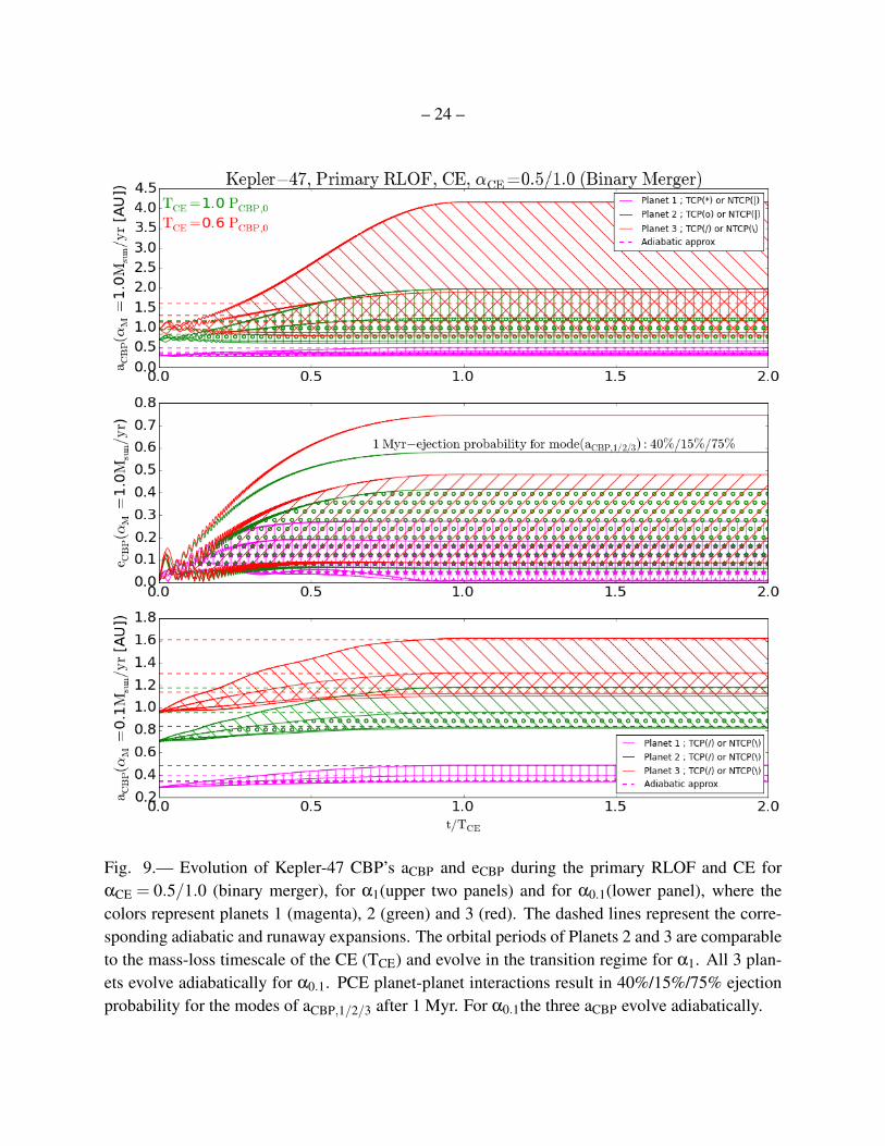
Fig. 9.— Evolution of Kepler-47 CBP’s aCBP and eCBP during the primary RLOF and CE forαCE = 0.5/1.0 (binary merger), for α1(upper two panels) and for α0.1(lower panel), where thecolors represent planets 1 (magenta), 2 (green) and 3 (red). The dashed lines represent the corre-sponding adiabatic and runaway expansions. The orbital periods of Planets 2 and 3 are comparableto the mass-loss timescale of the CE (TCE) and evolve in the transition regime for α1. All 3 plan-ets evolve adiabatically for α0.1. PCE planet-planet interactions result in 40%/15%/75% ejectionprobability for the modes of aCBP,1/2/3 after 1 Myr. For α0.1the three aCBP evolve adiabatically.

– 25 –

Fig. 10.— Same as Fig. 9 but for αCE = 3/5/10. The orbital periods of Planets 2 and 3 arecomparable to the CE mass-loss timescale TCE and evolve in the transition regime for α1; planet3 is ejected during the CE in 46%/81% of the simulations for NTCP/TCP respectively. For α1,planets 1/2/3 are ejected in 60%/15%/85% after 1-Myr. For α0.1their orbits evolve adiabaticallyand do not experience ejections.

– 26 –

as eCBP > 0.95. Specifically, planet 3 becomes unbound in 46% of the NTCP simulations, and in81% of the TCP simulations.

We note that during the primary CE stage, for the case of α1 the orbit of the inner CBP growsadiabatically while those of the outer do not (see upper panel of Fig. 10). This is because theorbital period of the inner planet is much shorter than the duration of TCE , while those of theouter two are comparable. Thus a multiplanet CB system can experience two regimes of planetaryorbital evolution during the same CE stage.

The dependence of aCBP,PCE and eCBP,PCE of Planet 2 on ∆θ0 is shown on Fig. 11 and 12.The planet’s orbit evolves adiabatically for α0.1(upper right panels), non-adiabatically for α1, andremains bound during the CE in both cases, regardless of ∆θ0.

Even if an ejection does not occur during the primary CE phase, aCBP,PCE and eCBP,PCE of allthree CBPs for α1 are such that the planets will continue to interact with each other after the end ofthe CE in such a way that further ejections/collisions are possible. To study the long-term evolutionof the system, we integrated the equations of motion for all five bodies (two stars and three planets)for 1 Myr, using the planets’ mode(aCBP,PCE ) and mode(eCBP,PCE ), and randomizing their initialarguments of pericenter and true anomalies. Any planet that achieves eCBP > 0.95 is markedas ejected and removed from the simulations, and collision is defined as planet-planet separationsmaller than dmin = RP,i +RP,j.

Overall, Planet 2 dominates the 1-Myr dynamical evolution and has the highest probabilityof remaining bound to the system. For αCE = 0.5/1 the modes of aCBP,1/2/3 have 40%/15%/75%ejection probability in 1 Myr. Where Planet 2 remains bound, it’s orbital elements remain mostlywithin the respective 68%-range of mode(aCBP,PCE,2) and mode(eCBP,PCE,2)11.

Here the modes of aCBP,1/2/3 have 60%/15%/85% ejection probability in 1 Myr, and the or-bital elements of Planet 2 again remain mostly within the 68%-range of mode(aCBP,PCE,2) andmode(eCBP,PCE,2).

4.4. Kepler-64

The binary consists of 1.53M�+ 0.41M� stars on a slightly-eccentric (ebin,0 = 0.22), 20-dayorbit which changes little in the first∼ 3 Gyr; the CBP has an initial orbit of 0.65 AU. The systemsevolves as follows.

11Except in one simulations where planet 1 is ejected, planet 2 migrates to a 5.67 AU, 0.71-eccentricity orbit, andplanet 3 migrates to a 0.55 AU, 0.66-eccentricity orbit.

– 27 –

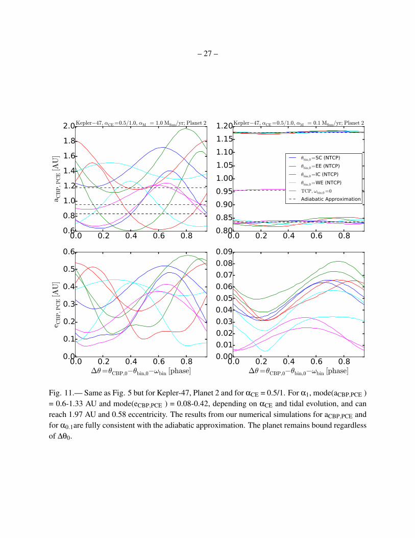
Fig. 11.— Same as Fig. 5 but for Kepler-47, Planet 2 and for αCE = 0.5/1. For α1, mode(aCBP,PCE )= 0.6-1.33 AU and mode(eCBP,PCE ) = 0.08-0.42, depending on αCE and tidal evolution, and canreach 1.97 AU and 0.58 eccentricity. The results from our numerical simulations for aCBP,PCE andfor α0.1are fully consistent with the adiabatic approximation. The planet remains bound regardlessof ∆θ0.

– 28 –

Fig. 12.— Same as Fig. 11 but for αCE = 3/5/10. For α1, mode(aCBP,PCE ) = 3.68/3.23 AU,mode(eCBP,PCE ) = 0.71/0.75 for TCP/NTCP, aCBP,PCE can reach 7.95 AU and eCBP,PCE can be ashigh as 0.89. The orbit of the planet evolves adiabatically for α0.1, and non-adiabatically for α1.The planet remains bound in both cases, regardless of ∆θ0.

– 29 –

4.4.1. The binary

The primary star fills its Roche lobe at t∼ 3.02 Gyr and the binary enters a primary CEstage. During this stage Ψ(α1) ≈ 0.03 and αcrit ≈ 32 M�/yr – much larger than α1and α0.1.However, for α1 the time of mass loss (TCE) is comparable to the orbital period of the CBP, i.e.TCE/PCBP ∼ 1.1−3.4, depending on αCE . Thus while the CBP is theoretically in the adiabaticregime, the comparable timescales result in a non-adiabatic dynamical response.

The binary merges as a First Giant Branch star and loses ∼ 20− 58% of its mass for αCE =0.5/1. In this regime β > βeject for αCE = 0.5, and for αCE = 1, TCP and the planet should remainbound in a runaway regime even at pericenter; β < βeject for αCE = 1.0 and NTCP, indicating apotential ejection of the CBP in a runaway regime. For αCE = 0.5 and 1 the system continues toslowly lose mass by the end of the BSE simulations (15 Gyr), thus aCBP,PCE expands adiabaticallyby up to a factor of 3.

For αCE = 3.0,5.0,10.0 the binary shrinks by a factor of 5− 25 and its mass decreases by∼ 65%; here β < βeject and the CBP should be ejected in a runaway regime. For αCE = 3 andTCP the system experiences a secondary RLOF at t∼ 6.2 Gyr and coalesces without mass loss (nochanges in aCBP or eCBP ). Except for αCE = 3 and TCP, the binary does not lose mass after theprimary CE.

The binary reaches 15 Gyr as either a merged COWD or a very close HeWD-MS star binary.

4.4.2. The CBP

On Fig. 13 we show the evolution of aCBP and eCBP for α1(red) and α0.1(green) respectivelyfor αCE = 0.5/1 (upper two panels) which result in a binary merger, and for αCE = 3/5/10 (lowertwo panels). The dependence of aCBP,PCE and eCBP,PCE on the initial phase difference between thebinary and the CBP (∆θ0) is shown on Fig. 14 for αCE = 0.5/1.0 and on Fig. 15 for αCE = 3/5/10.

Similar to Kepler-38, the orbital expansion of Kepler-64’s CBP is fully consistent with theadiabatic approximation for α0.1, and again the planet gains slight eccentricity (Table 10). Theoutcome for the case of α1 is quite diverse. Depending on ∆θ0, the planet can gain very higheccentricity, and even become ejected (eCBP > 0.95). This is shown as missing points in Fig.14 and 15. The Kepler-64 CBP can reach such eccentricities in ∼ 4% of our simulations forα1 and αCE = 3/5/10. Interestingly, for αCE = 0.5 and TCP, aCBP can decrease during the CEand Mode(aCBP,PCE ) = 0.6+0.6

−0.0 [AU] is smaller than the initial orbit aCBP,0 = 0.65 AU, though themode’s 68%-range is significant. On the other side of the spectrum, aCBP can reach up to ∼ 20 AUfor αCE =3/5/10 and NTCP.

– 30 –

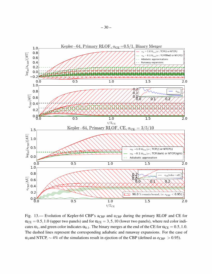
Fig. 13.— Evolution of Kepler-64 CBP’s aCBP and eCBP during the primary RLOF and CE forαCE = 0.5,1.0 (upper two panels) and for αCE = 3,5,10 (lower two panels), where red color indi-cates α1, and green color indicates α0.1. The binary merges at the end of the CE for αCE = 0.5,1.0.The dashed lines represent the corresponding adiabatic and runaway expansions. For the case ofα1and NTCP, ∼ 4% of the simulations result in ejection of the CBP (defined as eCBP > 0.95).

– 31 –

Fig. 14.— Same as Fig. 5 but for Kepler-64 and αCE = 0.5/1. For α1, mode(aCBP,PCE ) = 0.6-1.4AU and mode(eCBP,PCE ) = 0.16-0.62 depending on αCE and tidal evolution; aCBP,PCE can reach7.5 AU, and eCBP,PCE can reach 0.85. The results from our numerical simulations for aCBP,PCE andfor α0.1are fully consistent with the adiabatic approximation.

– 32 –

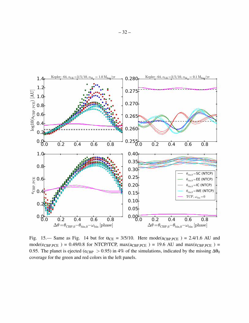
Fig. 15.— Same as Fig. 14 but for αCE = 3/5/10. Here mode(aCBP,PCE ) = 2.4/1.6 AU andmode(eCBP,PCE ) = 0.49/0.8 for NTCP/TCP, max(aCBP,PCE ) = 19.6 AU and max(eCBP,PCE ) =0.95. The planet is ejected (eCBP > 0.95) in 4% of the simulations, indicated by the missing ∆θ0

coverage for the green and red colors in the left panels.

– 33 –

4.5. Kepler-1647

The initial binary consists of 1.22M�+ 0.97M� stars on a slightly eccentric (ebin,0 = 0.15),11-day orbit which changes little in the first ∼ 5 Gyr. The CBP has an initial orbit of 2.7 AU. Themain stages of the evolution of the system are as follows.

4.5.1. The Binary

The primary star fills its Roche lobe at t∼ 5.4 Gyr and the binary enters a primary CE stage.During this stage Ψ(α1) ≈ 0.2 and αcrit ≈ 4.6 M�/yr – comparable to α1. Additionally, forNTCP and α0.1 the time of mass loss (TCE) is comparable to the orbital period of the CBP, i.e.TCE/PCBP ∼ 1.3/3.0 for αCE = 0.5/1.0 respectively. Thus the orbit of the CBP evolves in thetransition regime.

Compared to the other Kepler CBP systems, the binary star of Kepler-1647 experiences therichest evolution. For αCE = 0.5/1 the binary merges as a First Giant Branch star and loses ∼ 15−40% of its mass. In this regime β > βeject and the planet should remain bound in a runaway regimeeven at pericenter. The system continues to slowly lose mass by the end of the BSE simulations(15 Gyr), thus aCBP,PCE further expands (adiabatically) by up to a factor of 3.

For αCE = 3/5/10 the binary shrinks by a factor of 2−7 into a HeWD-MS star binary and itsmass decreases by∼ 45%, close to the critical mass loss for runaway ejection (0.5). Here β < βeject

and the CBP should remain bound even in a runaway regime.

The binary experiences a secondary RLOF and CE for αCE = 3/5/10 (see Table 6 for details),and its subsequent evolution can follow several paths. By the end of the BSE simulations, thebinary: a) merges without mass loss (i.e. no changes in aCBP,PCE and eCBP,PCE ) into a First GiantBranch for αCE = 3/5 and TCP, which by 15 Gyr evolves into a COWD; b) evolves into a PCEWD-WD binary (with mass loss, thus aCBP,PCE and eCBP,PCE changes) for αCE = 5 (and for NTCP)and for αCE = 10 (for both TCP and NTCP) which can experience a third and final RLOF triggeringa SN explosion (for αCE = 5/10 and TCP).

4.5.2. The CBP

The corresponding evolution of aCBP and eCBP for the primary RLOF, and for α1and α0.1isshown on Fig. 16. Unlike the previous systems, the α0.1case for Kepler-1647 represents an adia-batic evolution only for the TCP. For α0.1and NTCP, where TCE and PCBP are comparable for allαCE , the CBP’s orbit evolves in the transition regime (as it does for α1).

– 34 –

Specifically, for α0.1and NTCP the CBP reaches sufficiently high eccentricities (eCBP > 0.95)in∼ 5−25% of the simulations to be ejected from the system; for α1the planet is ejected in∼ 45−55% of the simulations. In addition, for αCE = 0.5/1 and NTCP, and for αCE = 3/5/10 and NTCP,aCBP can decrease during the primary CE phase and the corresponding mode of aCBP,PCE (1.6-2.3AU, depending on αCE , with a wide 68%-range) is smaller than the initial semi-major axis of theCBP (2.71 AU). Some of the simulations produce the opposite result, namely orbital expansionby up to a factor of ∼ 20 such that aCBP,PCE reaches ∼ 50 AU. The corresponding dependence ofaCBP,PCE and eCBP,PCE on ∆θ0 are shown in Fig. 17 and 18, where the missing ∆θ0 phase coveragein all panels represent planet ejection.

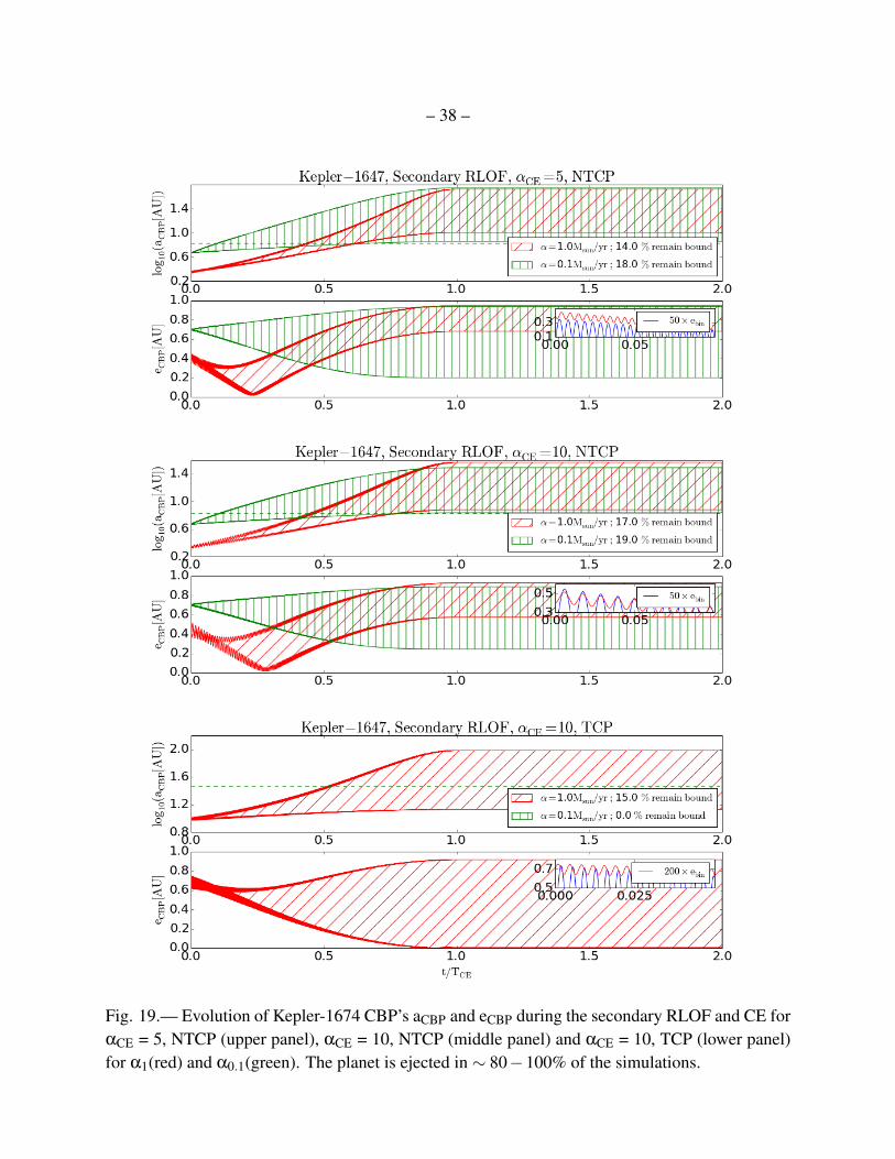
Using the respective abin,PCE and ebin,PCE, and the modes of aCBP,PCE and eCBP,PCE from theend of the preceding, primary RLOF as initial conditions, we further explore the evolution of theCBP for the secondary RLOF and CE stage for the three cases where the binary evolves into aWD-WD pair with mass loss: i) αCE = 5, NTCP; ii) αCE = 10, TCP; iii) αCE = 10, NTCP. Theresults are as follows.

During this secondary CE phase, for i) and ii) Ψ(α1)≈ 0.4 and αcrit ≈ 2.4 M�/yr – com-parable to α1, indicating that the CBP evolves in the transition regime. For iii) Ψ(α1)≈ 3.6,αcrit ≈ 0.3 M�/yr, and the evolution of the planet’s orbit is in the runaway regime. The time ofmass loss (TCE) is close to the orbital period of the CBP, i.e. TCE/PCBP ∼ 0.3−2.5. The binaryshrinks by a factor of ∼ 5−10 into a WD-WD pair, and loses ∼ 60−70% of its mass. As a result,β < βeject and the CBP should become unbound in a runaway regime.

The evolution of aCBP and eCBP during the secondary CE phase is shown in Fig. 19, wherethe upper panel represents case i) (αCE = 5, NTCP), the middle panel case ii) (αCE = 10, NTCP),and the lower panel – case iii) (αCE = 10, TCP). The CBP is ejected in more than ∼ 80% of thesimulations. For α1, the CBP’s aCBP expands to a mode value of ∼ 8−15 AU (depending on thescenario described above), with a maximum of up to 50-100 AU; the mode of eCBP is in the rangeof (0.5-0.75), reaching a maximum of 0.95. For α0.1, the CBP’s orbit can expand up to ∼ 30−50AU.

By the end of the BSE simulations, the CBP can remain bound only for ii) as the other twoscenarios trigger a SN shortly after the secondary CE.

4.6. Kepler-35

The system does not experience a CE evolution for Znominal, but the primary undergoes aRLOF and CE for Z−1σZ. Given the sensitivity of the binary evolution to the uncertainties in Z,here we outline the results for this system as well.

– 35 –

Fig. 16.— Evolution of Kepler-1647 CBP’s aCBP and eCBP during the primary RLOF and CEfor αCE = 0.5/1 (upper two panels) and for αCE = 3/5/10 (lower two panels), where red colorindicates α1, and green color indicates α0.1. The binary merges at the end of the CE (i.e. t = TCE)for αCE = 0.5/1. The dashed lines represent the corresponding adiabatic and runaway expansions.The CBP is ejected (eCBP > 0.95) in∼ 5−50% of the simulations depending on αCE and the tidalevolution, for both α1and α0.1. The latter case is non-adiabatic as TCE is comparable to the periodof the CBP at the start of the simulations (PCBP,0) and the CBP can expands to large orbits, gainingvery high eccentricities.

– 36 –

Fig. 17.— Same as Fig. 5 but for the primary CE stage of Kepler-1647 and αCE = 0.5/1. Heremode(aCBP,PCE ) = 1.6-3.9 AU, mode(eCBP,PCE ) = 0.26-0.72 depending on αCE and tidal evolution,max(aCBP,PCE ) = 37.5 AU and max(eCBP,PCE ) = 0.95. The planet is ejected in 47%/23% of theα1/α0.1 simulations, indicated by the missing ∆θ0 phase coverage for all but the magenta curves inthe left panels and points in the right panels.

– 37 –

Fig. 18.— Same as Fig. 17 but for αCE = 3/5/10. Mode(aCBP,PCE ) = 9.6/2.3 AU, mode(eCBP,PCE )= 0.7/0.4 for NTCP/TCP, max(aCBP,PCE ) = 47.1 AU and max(eCBP,PCE ) = 0.95. The planet isejected in 54%/4% of the α1/α0.1 simulations.

– 38 –

Fig. 19.— Evolution of Kepler-1674 CBP’s aCBP and eCBP during the secondary RLOF and CE forαCE = 5, NTCP (upper panel), αCE = 10, NTCP (middle panel) and αCE = 10, TCP (lower panel)for α1(red) and α0.1(green). The planet is ejected in ∼ 80−100% of the simulations.

– 39 –

4.6.1. The Binary

The binary consists of 0.88M�+ 0.81M� stars on a slightly-eccentric (ebin,0 = 0.15), 21-dayorbit which changes little in the first ∼ 13 Gyr. The CBP has an initial orbit of 0.6 AU.

The primary star fills its Roche lobe at t≈ 12.99 Gyr and the binary enters a primary CEstage. During this stage Ψ(α1)≈ 0.03 and αcrit ≈ 29.6 M�/yr – much larger than α1. As a resultof the CE, the binary merges as a First Giant Branch star and loses ∼ 35% of its mass for αCE =0.5; here β > βeject, and the planet should remain bound in a runaway regime. The system doesnot experience significant mass loss by the end of the BSE simulations (15 Gyr), thus no majorchanges in aCBP .

For αCE =1/3/5/10 the binary orbit shrinks by a factor of ∼ 2−10, loses ∼ 35% of its initialmass and evolves into a He-WD pair; here β > βeject, and the planet should remain bound in arunaway regime.

4.6.2. The CBP

Overall, for α0.1 the orbital evolution of the CBP is consistent with the adiabatic approxima-tion. For α1, mode(aCBP,PCE )∼ 0.8− 1 AU and the planet gains an eccentricity of 0.2-0.4; themin/max ranges can be significant. In particular, for αCE = 0.5, α1, and NTCP the CBP reachessufficiently high eccentricities (eCBP > 0.95) in ∼ 4% of the simulations to be ejected from thesystem; the CBP remains bound in all other cases. For α1 and NTCP aCBP,PCE can reach up to 7-10AU, with eCBP,PCE > 0.9.

5. Discussion and Conclusions

Several key results emerge from our study:

i) Five of the nine Kepler CBP hosts experience at least one RLOF and a CE phase for theirdefault parameters (masses, metallicities) by the end of our BSE simulations (15 Gyr); Kepler-35 experiences a primary RLOF for Z− 1σZ . Depending on the treatment of the CE stage, thebinaries either merge after primary or secondary CE (typically for αCE = 0.5/1) or evolve into veryshort-period WD-MS pairs (for αCE = 1/3/5/10)12; Kepler-1647 evolves into a WD-WD pair aftera secondary RLOF and CE for αCE = 5/10. Two systems trigger a double-degenerate Supernova

12Which can also merge for a secondary-triggered CE phase.

– 40 –

explosion – Kepler-34 for primary RLOF, and Kepler-1647 for a third RLOF and αCE = 5, TCP,and αCE = 10, NTCP. The binary systems lose a tremendous amount of mass – up to ∼ 60−70%– during the CE stages, and can shrink to sub-R�orbital separations.

ii) From the dynamical perspective presented here, Kepler CBPs predominantly remain boundto their host binaries after the respective CE phases even for mass-loss rates as high as 1.0 M� yr−1.There are only 4 scenarios where the respective CBP has a 100% probability of becoming unbound– 1) for Kepler-34 where the SN explosion occurs with the first CE; 2) for the secondary CE phaseof Kepler-1647 for α0.1, αCE = 10, TCP; 3) for the SN caused by the third RLOF of Kepler-1647,αCE = 5, NTCP; and 4) SN caused by the third RLOF of Kepler-1647, αCE = 10, TCP. In all otherscenarios (106 total, not accounting for the initial phase differences ∆θ0), the CBPs remain boundin the majority of cases (only Kepler-1647 has non-negligible ejection probability, again highlydependent on ∆θ0).

For mass-loss rates of 0.1 M� yr−1, the orbits of the CBPs evolve adiabatically – well re-produced by REBOUNDx – except for Kepler-1647. The orbital expansion of some of the Ke-pler CBPs is consistent with the adiabatic approximation even for mass-loss rates of 1.0 M� yr−1

(e.g. inner planet of Kepler-47, Kepler-64); in other cases, the mode of aCBP,PCE is smaller thanthe adiabatic approximation (i.e. Kepler-1647).

According to the analytical prescription, some systems should retain their CBPs even in arunaway mass-loss regime (Ψ� 1). Our code fully reproduces the runaway approximation forsingle-star systems.

iii) The transition regime (Ψ ∼ 0.1− 1) – where the evolution of some of Kepler CBPs fallsfor α1– is complex, and the final eccentricities and semi-major axes of the planets depend bothon the treatment of the CE stage (i.e. αCE , treatment of tides), and on the initial configuration ofthe system (i.e. ∆θ0). We find that the orbits of Kepler CBPs can expand by more than an orderof magnitude over the course of a single CBP year, reaching aCBP,PCE of tens of AU (during thesecondary CE of Kepler-1647 aCBP can expand from ∼ 10 AU to ∼ 100 AU, see Table 8).

Multiplanet CBP systems add yet another level of complexity as they can experience bothregimes simultaneously, e.g. where the orbit of the inner Kepler-47 CBP expands adiabatically, themiddle and outer CBP orbits grow non-adiabatically – all during the primary CE phase.

Overall, the CE-induced orbital evolution of CBPs is a dynamically rich and complex processin which a planet can migrate adiabatically during one CE phase, and non-adiabatically duringanother. As a result, a CBP cannot experience the same common envelope twice.

iv) If CE mass-loss rates are indeed high (e.g. ∼ 1.0 M� yr−1) – as suggested by theoreticalwork – and the orbits of Kepler-like CBPs evolve (and survive) according to our simulations, we

– 41 –

should expect to detect potentially highly eccentric planets orbiting PCE systems on very largeorbits. Alternatively, if Ψ� 1 then we should find PCE CBPs on low-eccentricity orbits. In-terestingly, recent observational efforts have produced a number of PCE Eclipse-Time Variations(ETV) CBP candidates on wide, notably eccentric orbits (e.g., Zorotovic & Schreiber (2013) andreferences therein), suggestion a possible connection with PCE Kepler-like CBPs.

On Fig. 20 we show aCBP,PCE vs eCBP,PCE of Kepler’s CBPs13 and compare them to those ofthe PCE ETV CBP candidates14. We caution that the comparison is not direct as neither the CEstages of the different Kepler systems occur all at the same time, nor do the PCE ETV CBPs haveidentical ages. Instead, given the handful of known targets – Kepler’s nine compared to estimatedmillions of similar CBPs (Welsh et al. 2012); a dozen PCE ETV CBPs – the lower two panels onthe figure portray a potential distribution of an underlying PCE CBP population with a range ofages and evolutionary stages.

Overall, the PCE orbital configurations of Kepler’s CBPs are qualitatively consistent withthose of the observed population of the currently known PCE ETV CBP candidates15. Thus ourresults both assist in interpreting the nature of these candidates and in guiding future observationalefforts to discover new systems. Such discoveries will provide a deeper understanding of the evolu-tion of planets in binary star system, and also much-needed observational constraints on the stellarastrophysics of the complex CE phase, as “CE is one of the most important unsolved problemsin stellar evolution”, according to Ivanova et al. (2013),“and is arguably the most significant andleast-well-constrained major process in binary evolution” (but also see Taam & Sandquist (2000);Taam & Ricker (2010) andWebbink (2008) for alternative reviews).

vi) A CB body gravitationally perturbs its host binary star, and if the latter is eclipsing theseperturbations can be manifested as deviations from linear ephemeris in the measured stellar eclipsetimes. The cause of these variations can be either dynamical, where the third body’s influencechanges the orbital elements of the binary star, or a light travel-time effect (LTTE), where the ter-tiary object and the binary revolve around a common center of mass. ETVs are indeed a powerful– and highly productive – method to discover and study stellar triple and higher order systems(e.g. Orosz 2015; Borkovits et al. 2015, and references therein), and have recently been used tostudy CBPs as well. In particular, the former effect has been measured for several of the Ke-pler CBP systems and used to constrain the respective planetary masses (Doyle et al. 2011; Welshet al. 2012; Kostov et al. 2016). The latter effect has been suggested as the cause for measured

13For Kepler-47 we only show the middle planet (Planet 2) as it has the highest probability to survive both the CEphase and subsequent planet-planet interactions.

14For those candidates that do not have published eccentricities we set the respective eCBP to zero.

15With the caveat that the latter are much too massive.

– 42 –

Fig. 20.— Upper six panels: aCBP,PCE vs eCBP,PCE for Kepler’s CBPs for various CE treatments(green, blue and red symbols) and initial conditions (∆θ0 = 0÷1), along with the respective ejec-tion probabilities; lower two panels: comparison between Kepler’s aCBP,PCE vs eCBP,PCE and thoseof the currently known PCE ETV CBPs candidates (black symbols) at the ends of the respectiveKepler CEs (left) and at the end of our BSE simulations (15 Gyr, right). Given the associated ob-servational and numerical uncertainties, our forward-evolution results are qualitatively consistentwith the observed aCBP,PCE vs eCBP,PCE distributions. See text for details.

– 43 –

ETVs for a number of PCE EB systems with proposed CB companions (as mentioned above, alsosee Volschow et al. (2016) and references therein).

Assuming that the orbits of the Kepler CBPs studied here evolve only dynamically and theirmasses remain constant (i.e. no changes due to, for example, interactions with a CE-triggeredCB disk), it is informative to evaluate the respective planets’ ETV-based detectability after the CEstages of the relevant systems. To calculate the expected amplitudes of the two effects discussedabove, Adyn and ALTTE, we use the formalism of Borkovits et al. (2012, 2015).

The respective amplitudes and periods for Kepler-35 (Mp= 0.13MJup) and Kepler-1647 (Mp=1.5MJup) – the only two systems with well-constrained CBP masses – are listed in Table 11 (for therespective range of binary and CBP parameters listed in Tables 8), and compared to the detectedsignals for the two PCE CBP candidates NN Ser and HW Vir. As seen from Table 11, detectionof such ETVs is feasible both in terms of the amplitudes and periods of the expected signal, whichare qualitatively similar to the ETV signals of the two PCE CBP candidates.

Another option for the detection of a PCE CBP is to directly image the planet. The benefitsfor such detection are two fold: a) the contrast ratio between the binary and the CBP decreasesafter each CE phase as the primary and/or secondary evolves from a luminous MS star to a muchfainter WD; b) the angular separation between the binary and the CBP increases16 (e.g. Hardyet al. 2015). There is potentially a third benefit, where the CBP can accrete mass after the CEstage (e.g. Zorotovic & Schreiber 2013; Bear & Soker 2014) and becomes brighter, thus furtherdecreasing the contrast ratio.

Recently, Hardy et al. (2015) used VLT/SPHERE to observe the V471 Tau system – an eclips-ing binary star with measured ETVs – with the goal to directly image a sub-stellar mass CB can-didate suspected to be the cause of the ETVs. Given the known age of the system, and the massesof the binary and the CB candidate, direct detection of such tertiary body should have been wellwithin the capabilities of the instrument. Hardy et al. (2015), however, report a null detection,casting doubt on the interpretation of the measured ETV signal (but see Vaccaro et al. (2015)for alternative explanation). Nevertheless, based on our results for the dynamical survivability ofCBPs around evolving binary stars, and on estimates of the occurrence rates of planets orbitingshort-period MS binary stars (e.g. Welsh et al. 2012), we encourage the continuation of such directimaging efforts – aimed at both PCE, very short-period binaries, and also at PCE WD-coalescedbinaries where the contrast ratio is even more favorable.

vii) The closer a planet’s orbit is to a single star during the MS stage, the worst its prospectsare for survival when the star ascends the RGB and AGB. For example, Mercury, with an orbit of

16Such that the minimum increase is typically for adiabatic orbital expansion.

– 44 –

0.46 AU will be destroyed as the Sun evolves off the main sequence (e.g. Schroder&Connon Smith2008. In contrast, our results suggest that despite their dramatic evolution, close binary stars mayin fact be better for the survival of planets compared to single stars. For example, the Kepler-38CBP has an initial orbital separation similar to Mercury’s, and yet it survives the evolution of abinary star with a total mass of ∼ 1 M�. A CBP with an even smaller orbit – as small as 0.3-0.35 AU – can survive the evolution of 1.3-1.4 M� (total mass) central binary star as is the case forthe inner planet in Kepler-47. A planet with the same orbit around a single star of the same masswill have no chance for survival (Villaver & Livio 2007). Thus despite being a disruptive stage forthe binary star itself, the CE phase may in fact promote planet survivability.

viii) With the exception of Kepler-1647, the Kepler CBPs currently orbit their binary starhosts within a factor of 2 of the critical limit for dynamical stability (Holman & Wiegert (1999),HW hereafter), i.e. aCBP,0(1− eCBP,0)/acrit,0 ∼ 2 (the factor for Kepler-1647 is ∼ 7). However,as the binaries shrink and lose mass during the CE, and the planets migrate to larger, eccentricorbits, this ratio will change. To calculate acrit,PCE – the PCE critical limits (for those scenarioswhere the binaries do not coalesce, i.e. αCE = 3/5/10) – we use Eqn. 3 from HW using a bi-nary mass ratio µ = MA,PCE/(MA,PCE +MB,PCE)

17. As the CE phases result in a variety of abin ,aCBP,PCE and eCBP,PCE , here we quote only the most constraining critical limits, i.e. where therespective separation between abin and aCBP,PCE (1− eCBP,PCE ) is at a minimum. For α1, the lim-its for Kepler-38, Kepler-47, Kepler-64, Kepler-1647 (NTCP) and Kepler-1647 (TCP) in terms ofaCBP,PCE (1− eCBP,PCE )/acrit,PCE are 3.3, 7.9, 5.3, 15.9, 14.7 and 29.5 respectively, indicating thatthe CBPs remain in a dynamically-stable regime.

While it is beyond the scope of this study, we note that tidal evolution of the binary orbit priorto the CE phase may affect the CBP orbits. Specifically, as most of the planets are currently orbitingclose to their host binaries, a pre-CE decay in abin means that strong mean motion resonances(MMR) may sweep over the planet, leading to eccentricity excitation and potential destabilization.As an example, abin of Kepler-38 decreases from 31.6 R�to 24.6 R�prior to the CE phase for TCP(see Table 4), indicating that the CBP’s orbit crosses 6:1, 7:1 and 8:1 MMR. The MMR crossingsare a) 7:1, 8:1, 9:1 for Kepler-47 (Planet 1); b) 7:1 through 11:1 for Kepler-64; and c) 99:1 through116:1 for Kepler-1647.

ix) “...It is interesting to consider the situation at a much earlier time in the past when theprimary was near the zero-age main sequence...”, note Orosz et al. (2012a) for the case of Kepler-38b, “The primary’s luminosity would have a factor≈ 3 smaller...”. While Kepler-38b is currentlycloser to its binary host than the inner edge of the habitable zone (HZ) for the system, four of theKepler CBPs (Kepler-16, Kepler-47c, Kepler-453, Kepler-1647) reside in the HZ. As their host

17Since the primary star becomes the less massive component of the binary after the CE phase.

– 45 –

binaries evolve, however, the location of the HZ will change.

Unlike the case for single stars where both the HZ and a (surviving) planet’s orbit will expandduring the RGB and AGB stages (Villaver & Livio 2007), as a close binary star evolves througha CE stage the HZ can shrink while its CBP migrates outwards. The shrinking is caused by theluminosity drop of the central binary as one of its stars rapidly transitions from the MS to a compactobject. Thus a CBP residing in the HZ during the pre-CE binary will leave the zone after the CEphase (e.g. Kepler-1647), whereas a CBP that is initially interior to the HZ may migrate to a PCEorbit coinciding with the PCE HZ.

Consequently, it would be equally interesting to consider the configuration of a CBP systemat a much later time in the binary evolution. For example, the current orbital configuration ofKepler-35b is such that the planet’s orbit is internal to the HZ (Welsh et al. 2012). However, asits host binary evolves through the CE phase, for αCE = 1/3/5/10 the primary star evolves intoa HeWD (while the secondary remains on the MS as a 0.81 M� star) and the CBP migratesto mode(aCBP,PCE ) = 0.84−1.0 AU,mode(eCBP,PCE ) = 0.0−0.4 (see Tables 8). This migrationplaces the planet near the conservative HZ of 0.98−1.77 AU (for 1 M⊕ (Kopparapu et al. 2014),using the luminosity, 0.4 LSun, and temperature of the secondary star, 5200 K (Welsh et al. 2012),and ignoring the flux contribution of the WD).

5.1. Limitations

The results presented here are based on the assumptions that the CBPs do not interact with thematerial ejected from their binary star. However, numerical studies have indicated that this materialis neither lost isotropically from the binary during the CE phase, nor does it all become unbound.Instead, 1−10% of the ejecta may fall back into a CB disk according to Kashi & Soker (2011), andPassy et al. (2012) suggest that ∼ 80% of the ejected material may remain gravitationally boundto the binary (also see Kuiper 1941; Shu et al. 1979, and Pejcha et al. 2016 for mass loss outflowsthrough the L2 Lagrange point18). Either of these scenarios would significantly complicate thedynamical evolution of the system as the CBP could accrete material and gain mass, and alsoexperience migration similar to that during planetary formation19. Such accretion of material ofa different specific angular momentum will change the orbital evolution of the planet, as willgravitational interaction with the bulk gas in an accretion-favorable environment such as a CB

18Mass-loss through L2 results in several possible outcomes, e.g. isotropic or equatorial wind, CB disk – for detailssee Tab. 1, Fig. 12 and 13 of Pejcha et al. 2016.

19There are, however, two potential benefits of the former in terms of detection: a more luminous planet would bemore amenable to direct imaging efforts; and a more massive planet would cause stronger ETVs.

– 46 –

disc. Additionally, interactions between CBPs and the CE ejecta of close binary stars (includingejection or destruction of the planets) may also play an important role in the elusive mechanismsresponsible for the shaping, morphology and chemistry of planetary nebulae (see Bear & Soker(2016) for triple star origin of asymmetric planetary nebulae; for recent reviews see Zijlstra (2014)and Jones (2015), and references therein). We note that the CE-triggered dynamical disturbancesdiscussed here occur on timescales of ∼ 1 year, and are thus ‘instantaneous’ compared to anysubsequent planet migration, which occurs on much longer timescales.

PCE CB disks are also suspected to trigger a new episode of planet formation, i.e. a secondgeneration scenario (e.g. Verhoelst et al. 2007; Perets 2010; Tutukov & Fedorova 2012 and refer-ences therein), and have also been suggested to be the birthplace of several PCE CBP candidates(Volschow, Banerjee, & Hessman 2013; Schleicher&Dreizler 2014)20. Indeed, a recent discoveryof dust around NN Ser supports the presence of a remnant PCE disc (Hardy et al. 2016). Al-ternatively, based on angular momentum constraints Bear & Soker (2014) argue that these CBPcandidates formed together with their host binary stars (i.e. first generation). Mixed scenarios,where the CBP forms with the binary, survives the CE stage and subsequently acts as a seed forthe accretion of more mass, are also possible (Armitage & Hansen 1999; Perets 2010; Schleicheret al. 2015), showcasing the complexity and diversity of the formation and evolution mechanismsof planets around close binary stars.

These complications are, however, beyond the scope of our study and we defer their imple-mentation to future work.

5.2. Conclusions

We have presented numerical studies of the dynamical evolution of the nine Kepler CBPsystems as their host binary stars undergo CE phases. Five of the systems undergo at least oneRLOF and CE phases; Kepler-1647 experiences three RLOFs. Two systems trigger a double-degenerate SN explosion. Depending on the treatment of the CE phase (i.e. efficiency and tidalevolution), the binaries either coalesce or shrink into very close WD-MS or WD-WD pairs ofstars. Despite the dramatic reconfiguration of the binary stars during these violent evolutionaryphases, the planets predominantly survive the CE stage even for mass-loss rates of 1 M� yr−1.The PCE orbital configurations of these CBPs depend on the rate at which the binary loses mass.For mass-loss rates of 1 M� yr−1 the CBPs migrate non-adiabatically outwards to highly eccentricorbits, while for slower mass-loss rates (0.1 M� yr−1) our simulations reproduce the expected

20Second generation has also been proposed for the origin of the first detected exoplanet (Wolszczan & Frail 1992).

– 47 –

adiabatic orbital expansion. Overall, the PCE semi-major axes and eccentricities of Kepler CBPsare qualitatively consistent with those of the currently known PCE CBP candidates. The modeof orbital expansion depends on the particular configuration of the system, such that a CBP canmigrate adiabatically during the primary CE stage, but non-adiabatically during the secondary CEstage. Multiplanet CBP systems can experience both modes simultaneously, i.e. an inner planetcan migrate adiabatically while an outer does so non-adiabatically – both occurring during thesame CE stage. Our results also indicate that planets are more likely to survive around evolvingclose binary stars than around evolving single stars, thus improving the discovery prospects forCBPs in PCE systems.

We thank the anonymous referee for the insightful comments that helped us improve thispaper. The authors are grateful to Jarrod Hurley and Marten van Kerkwijk for valuable discussions.VBK gratefully acknowledges support by an appointment to the NASA Postdoctoral Program atthe Goddard Space Flight Center. DT was supported by a postdoctoral fellowship from the Centrefor Planetary Sciences at the University of Toronto at Scarborough, and is grateful for additionalsupport from the Jeffrey L. Bishop Fellowship. This work was supported in part by NSERC grantsto RJ. We acknowledge conversations with Daniel Fabrycky, Nader Haghighipour, Kaitlin Kratter,Boyana Lilian, Jerome Orosz, William Welsh.

REFERENCES

Adams, F. C., Anderson, K. R., & Bloch, A. M. 2013, MNRAS, 431, 438

Adams, F. C., & Bloch, A. M. 2013, ApJ, 777, 30

Armitage, P. J. & Hansen, B. M. S. 1999, Nature, 402, 633

Bear, E. & Soker, N. 2014, MNRAS, 444, 1698

Bear, E. & Soker, N. 2016, 2016arXiv160608149B

Borkovits, T., Derekas, A., Kiss, L. L. et al. 2012, MNRAS, 428,1656

Borkovits, T., Rappaport, S., Hajdu, T., & Szakovicz, J. 2015, MNRAS, 448, 948

Borkovits, T., Hajdu, Szakovicz, J., et al. 2016, MNRAS, 455, 4136

De Marco, O. et al. 2003, ”Revista Mexicana de Astronomia y Astrofisica”, 27, 18, in Revista Mex-icana de Astronomia y Astrofisica Conference Series, ed. M. Reyes-Ruiz & E. Vazquez-Semadeni, 24/30, 2009, Journal of Physics Conference Series, 172, 012031

– 48 –

Doyle, L. R., Carter, J. A., Fabrycky, D. C., et al. 2011, Science, 333, 6049

Duncan, M. J. & Lissauer, J. J. 1998, Icarus, 134, 303

Farihi, J. 2016, NewAR, 71, 9

Hadjidemetriou, J. D. 1963, Icarus, 2, 440

Hardy, A. et al. 2015, ApJ, 800, 24

Hardy, A., Schreiber, M. R., Parsons, S. G., et al. 2016, http://arxiv.org/abs/1604.05808

Hilditch, R. W. 2001, An Introduction to Close Binary Stars, by R. W. Hilditch, pp. 392. ISBN0521241065. Cambridge, UK: Cambridge University Press, March 2001.

Holman, M. J., & Wiegert, P. A. 1999, AJ, 117, 621

Hurley, J. R., Pols, O. R., & Tout, C. A. 2000, MNRAS, 315, 543

Hurley, J. R., Tout, C. A., & Pols, O. R. 2002, MNRAS, 329, 897

Iaconi, R. et al. 2016, arXiv:160301953

Ivanova, N. et al. 2013, A&A Rev., 21, 59

Jones, D. 2015, EAS, 71, 113

Kashi, A. & Soker, N. 2011, MNRAS, 417, 1466

Kippenhahn, R. & Wiegert, A. 1990, ”Stellar Structure and Evolution”, Springer-Verlag, ISBN3-540-50211-4

de Kool, M. 1990, ApJ, 358, 189

Kopparapu, R. K.; Ramirez, R. M.; SchottelKotte, J.; Kasting, J. F.; Domagal-Goldman, S.; Eymet,V. 2014, ApJ, 787, 2

Kostov, V. B., McCullough, P. R., Hinse, T. C., et al. 2013, ApJ, 770, 52

Kostov, V. B., McCullough, P. R., Carter, J. A., et al. 2014, ApJ, 784, 14

Kostov, V. B., Orosz, J., Welsh, W., et al. 2016, ApJ, 827, 86

Kratter, K., & Perets, H. B. 2012, ApJ, 753, 91

Kuiper, G. P. 1941, ApJ, 93, 133

– 49 –

Livio, M. & Soker, N. 1984, MNRAS, 208, 763

Mustill, A., Marshall, J. P., Villaver, E. et al. 2013, MNRAS, 436, 2515

Nandez, J. L. A., Ivanova, N., & Lombardi, J. C. Jr. 2014, ApJ, 786, 39

Orosz, J. A., Welsh, W. F., Carter, J. A., et al. 2012a, Science, 337, 1511

Orosz, J. A., Welsh, W. F., Carter, J. A., et al. 2012b, ApJ, 758, 87

Orosz, J. A. 2015, ASPC, 496, 55

Paczynski, B. 1976, BAAS, 8, 442

Papaloizou, J. C. B., & Larwood, J. .D. 2000, MNRAS, 315, 823

Pejcha, O.; Metzger, B. D.; & Tomida, K. 2016, MNRAS, 461, 3

Portegies Zwart, S. 2013, MNRAS, 429, 45

Passy, J.-C. et al. 2012, ApJ, 744, 52,

Raghavan, D.; McAlister, H. A.; Henry, T. J. et al. 2010, ApJS, 191, 1

Rasio, F., & Livio, M. 1996, ApJ, 471, 366;

Reffert, S. et al. 2015, A&A, 574, 116

Rein, H. & Liu, S.-F. 2012, A&A, 537, 128

Rein, H. & Spiegel, D. S. 2015, MNRAS, 448, 58

Ricker, P. M. & Taam, R. E. 2008, ApJ, 672, 41

Ricker, P. M. & Taam, R. E. 2012, ApJ, 746, 74

Perets, H. 2010, arXiv1001.0581

Sandquist, E. L. et al. 1998, ApJ, 500, 909

Schleicher , D. R. G., & Dreizler, S. 2014, A&A, 563, 61

Schleicher, D. R. G., Dreizler, S., Volschow, M. et al. 2015, AN, 336, 458

Schroder, K.-P., & Connon Smith, R. 2008, MNRAS, 386, 15

Schwamb, M. E., Orosz, J. A., Carter, J. A. et al. 2013, ApJ, 768, 127

– 50 –

Shu, F. H., Anderson, L., & Lubow, S. H. 1979, ApJ, 229, 223

Taam, R. E. & Ricker, P. M. 2010, NewAR, 54, 65

Taam, R. E. & Sandquist, E. L. 2000, ARAA, 38, 113

Tutukov, A. V. & Fedorova, A. V. 2012, ARep, 56, 305

Vaccaro, T. R., Wilson, R. E., Van Hamme, W. & Terrell, D. 2015, ApJ, 810, 157

Veras, D., Wyatt, M. C., Mustill, A. J. et al. 2011, MNRAS, 417, 2104

Veras, D. & Tout, C. A. 2012, MNRAS, 422, 1648

Veras, D. 2016, RSOS, 3.0571

Verhoelst, T., van Aarle, E., & Acke, B. 2007, A&A, 470, 21

Villaver, E. & Livio, M. 2007, ApJ, 661, 1192

Volschow, M., Banerjee, R, & Hessman, F. V. 2014, A&A, 562, 19

Volschow, M., Schleicher, D. R. G., Perdelwitz, V., & Banerjee, R. 2016, A&A, 587, 34

Webbink, R. F. 2008, ASSL, 352, 233

Welsh, W. F.; Orosz, J. A.; Carter, J. A., et al. 2012, Nature, 481, 475

Welsh, W. F. et al. 2015, ApJ

Wittenmyer, R.A. et al. 2016, ApJ, 818, 35

Wolszczan, A., & Frail, D. A. 1992, Nature, 355, 145

Zijlstra, A. A. 2014, RMxAA, 51, 221

Zorotovic, M. & Schreiber, M. R. 2013, A&A, 549, 95

This preprint was prepared with the AAS LATEX macros v5.2.

– 51 –

A.List of Abbreviations and Parameters

BSE: Binary Star Evolution codeCE: Common EnvelopeCBP: CircumBinary PlanetEB: Eclipsing BinaryNTCP: No Tidal Circularization Path (tides “OFF” in BSE)PCE: Post-Common EnvelopeRLOF: Roche Lobe OverflowTCP: Tidal Circularization Path (tides “ON” in BSE)

αM : Common Envelope mass-loss rateα1: 1 M�/yr mass-loss rateα0.1: 0.1 M�/yr mass-loss rateαcrit: Critical Common Envelope mass-loss rateαCE : Common Envelope efficiency parameteraCBP,0: Initial semi-major axis of the circumbinary planetsaCBP,PCE: Semi-major axis of the circumbinary planets at the end of the Common Envelopeβ: Ratio between initial and final mass of the systemβeject: Runaway ejection ratio between initial and final mass of the systemeCBP,0: Initial eccentricity of the circumbinary planetseCBP,PCE: Eccentricity of the circumbinary planets at the end of the Common Envelope phaseψ: Common Envelope mass-loss indexTCE : Common Envelope mass-loss timescale

– 52 –

Table 1: BSE Parameter SpaceParameter Explored Values

M1 M1,M1 +3σ,M1−3σ

M2 M2,M2 +3σ,M2−3σ

Metallicity Z Z,Z +1σ,Z +2σ,Z +3σ,Z−1σ,Z−2σ,Z−3σ

αCE 0.5,1.0,3.0,5.0,10.0Tides OFF, ON

de Kool CE Model OFF, ONForce Corotation OFF, ON

Note: Values denoted in boldface represent the default parameters used in our simulations.

– 53 –

Table 2: BSE Stellar TypesStellar Type Description

0 Deeply or fully convective low-mass MS star1 Main Sequence star2 Hertzsprung Gap (HG)3 First Giant Branch (GB)4 Core Helium Burning (CHeB)5 First/Early Asymptotic Giant Branch (EAGB)6 Second/Thermally Pulsing Asymptotic Giant Branch (TPAGB)7 Main Sequence Naked Helium star (HeMS)8 Hertzsprung Gap Naked Helium star (HeHG)9 Giant Branch Naked Helium Star (HeGB)

10 Helium White Dwarf (HeWD)11 Carbon/Oxygen White Dwarf (COWD)12 Oxygen/Neon White Dwarf (ONeWD)13 Neutron Star (NS)14 Black Hole (BH)15 Massless Supernova/Massless Remnant

Table 3: BSE Output Evolution StagesEvolutionary Stage Label Description

INITIAL Initial configurationKW CHNGE Stellar type changeBEG RCHE Begin Roche lobe overflowEND RCHE End Roche lobe overflowCONTACT Contact systemCOELESCE Coalescence of starsCOMENV Common-envelope systemGNTAGE New giant star from CE; appropriate age and initial mass set to match core-mass and stellar mass

NO REMNT No remnantMAX TIME Max evolutionary time reached; end of programDISRUPT System is disrupted

BEG SYMB Begin symbiotic systemEND SYMB End symbiotic system

BEG BSS Begin blue stragglers

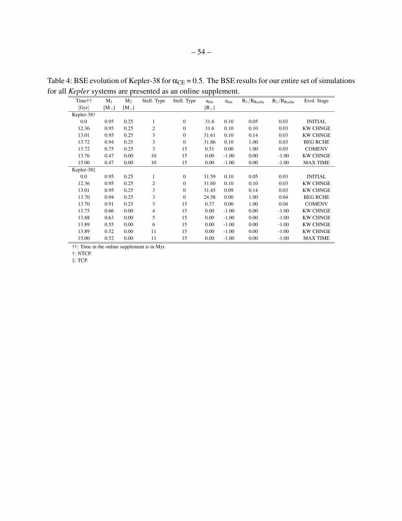
– 54 –

Table 4: BSE evolution of Kepler-38 for αCE = 0.5. The BSE results for our entire set of simulationsfor all Kepler systems are presented as an online supplement.

Time†† M1 M2 Stell. Type Stell. Type abin ebin R1/RRoche R1/RRoche Evol. Stage[Gyr] [M�] [M�] [R�]

Kepler-38†0.0 0.95 0.25 1 0 31.6 0.10 0.05 0.03 INITIAL

12.36 0.95 0.25 2 0 31.6 0.10 0.10 0.03 KW CHNGE13.01 0.95 0.25 3 0 31.61 0.10 0.14 0.03 KW CHNGE13.72 0.94 0.25 3 0 31.86 0.10 1.00 0.03 BEG RCHE13.72 0.75 0.25 3 15 0.51 0.00 1.00 0.03 COMENV13.76 0.47 0.00 10 15 0.00 -1.00 0.00 -1.00 KW CHNGE15.00 0.47 0.00 10 15 0.00 -1.00 0.00 -1.00 MAX TIME

Kepler-38‡0.0 0.95 0.25 1 0 31.59 0.10 0.05 0.03 INITIAL

12.36 0.95 0.25 2 0 31.60 0.10 0.10 0.03 KW CHNGE13.01 0.95 0.25 3 0 31.45 0.09 0.14 0.03 KW CHNGE13.70 0.94 0.25 3 0 24.58 0.00 1.00 0.04 BEG RCHE13.70 0.91 0.25 3 15 0.37 0.00 1.00 0.04 COMENV13.75 0.66 0.00 4 15 0.00 -1.00 0.00 -1.00 KW CHNGE13.88 0.63 0.00 5 15 0.00 -1.00 0.00 -1.00 KW CHNGE13.89 0.55 0.00 6 15 0.00 -1.00 0.00 -1.00 KW CHNGE13.89 0.52 0.00 11 15 0.00 -1.00 0.00 -1.00 KW CHNGE15.00 0.52 0.00 11 15 0.00 -1.00 0.00 -1.00 MAX TIME

††: Time in the online supplement is in Myr.†: NTCP.‡: TCP.

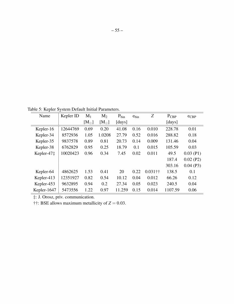
– 55 –

Table 5: Kepler System Default Initial Parameters.Name Kepler ID M1 M2 Pbin ebin Z PCBP eCBP

[M�] [M�] [days] [days]

Kepler-16 12644769 0.69 0.20 41.08 0.16 0.010 228.78 0.01Kepler-34 8572936 1.05 1.0208 27.79 0.52 0.016 288.82 0.18Kepler-35 9837578 0.89 0.81 20.73 0.14 0.009 131.46 0.04Kepler-38 6762829 0.95 0.25 18.79 0.1 0.015 105.59 0.03

Kepler-47‡ 10020423 0.96 0.34 7.45 0.02 0.011 49.5 0.03 (P1)187.4 0.02 (P2)

303.16 0.04 (P3)Kepler-64 4862625 1.53 0.41 20 0.22 0.031†† 138.5 0.1

Kepler-413 12351927 0.82 0.54 10.12 0.04 0.012 66.26 0.12Kepler-453 9632895 0.94 0.2 27.34 0.05 0.023 240.5 0.04

Kepler-1647 5473556 1.22 0.97 11.259 0.15 0.014 1107.59 0.06

‡: J. Orosz, priv. communication.††: BSE allows maximum metallicity of Z = 0.03.

– 56 –

Table 6: Binary Evolution from BSE. The numbers quoted in parenthesis for the time represent thecorresponding range, obtained from BSE for Z±3σZ (see text for details). The typical range forM1and M2 is ∼ 0.01−0.1 M�, and ∼ 0.1−1 R� for abin.

αCE Tides M1 M2 abin ebin Time RLOF§ Notes[MSun] [MSun] [R�] [Gyr]

Kepler-34– – 1.05 1.02 49.2 0.52 0

0.5/1/3/5/10 NTCP – – – – 9.64(1.7) DD SN0.5/1/3/5/10 TCP – – – – 9.66(1.7) DD SN†

Kepler-38– – 0.95 0.25 31.6 0.1 0

0.5 NTCP 0.76 – – – 13.72(0.6) CE + Merger0.5 TCP 0.91 – – – 13.70(0.6) CE + Merger

1/3/5/10 NTCP 0.27 0.25 1.0/2.8/4.5/7.8 – 13.72(1.2) CE1/3/5/10 TCP 0.25 0.25 0.7/2.0/3.2/5.7 – 13.70(1.1) CE§§

Kepler-47– – 0.96 0.34 17.5 0.02 0

0.5 NTCP 1.08 – – – 12.03(1.3) CE + Merger0.5 TCP 1.14 – – – 11.99(1.3) CE + Merger1.0 NTCP 0.78 – – – 12.03(1.5) CE + Merger1.0 TCP 0.96 – – – 11.99(1.5) CE + Merger

3/5/10 NTCP 0.23 0.34 1.7/2.6/4.5 – 12.03(1.7) CE3/5/10 TCP 0.21 0.34 1.2/1.9/3.4 – 11.99(1.6) CE

Kepler-64– – 1.53 0.41 38.7 0.22 0

0.5 NTCP 1.53 – – – 3.02(0.3) CE + Merger0.5 TCP 1.68 – – – 3.02(0.3)†† CE + Merger1.0 NTCP 0.8 – – – 3.02(0.3) CE + Merger1.0 TCP 1.35 – – – 3.02(0.3) CE + Merger

3/5/10 NTCP 0.28 0.41 2.4/3.9/7.0 – 3.02(0.3) CE3/5/10 TCP 0.26 0.41 1.6/2.6/4.7 – 3.02(0.3) CE

3 TCP 0.67 – – – 6.20(0.4) CE‡ + MergerKepler-1647

– – 1.22 0.97 27.4 0.15 00.5 NTCP 1.81 – – – 5.45(0.45) CE + Merger0.5 TCP 1.87 – – – 5.44(0.46) CE + Merger1.0 NTCP 1.28 – – – 5.45(0.44) CE + Merger1.0 TCP 1.45 – – – 5.44(0.43) CE + Merger

3/5/10 NTCP 0.25 0.97 4.0/6.2/10.1 – 5.45(0.45) CE3/5/10 TCP 0.24 0.97 3.6/5.4/8.9 – 5.44(0.36) CE

3 TCP 1.16 – – – 6.07(0.35) CE‡ + Merger5 NTCP 0.25 0.17 0.6 – 12.06(0.9) CE‡

5 NTCP – – – – 12.93(1.0) DD SN5 TCP 1.15 – – – 9.85(0.5) CE‡ + Merger

10 NTCP 0.25 0.2 1.9 – 12.27(1.1) CE‡

10 TCP 0.24 0.16 0.7 – 11.86(0.9) CE‡

10 TCP – – – – 13.99(0.5) DD SNKepler-35 (Z−1σZ)

– – 0.88 0.81 37.9 0.14 00.5 NTCP 1.1 – – – 12.99(1.44) CE + Merger0.5 TCP 1.09 – – – 12.99(1.44) CE + Merger

1/3/5/10 NTCP 0.29 0.81 3.5/8.8/12.7/19.1 – 12.99(1.44) CE1/3/5/10 TCP 0.28 0.81 3.1/7.9/11.5/17.4 – 12.99(1.44) CE

§: Roche Lobe OverFlow.†: Double-degenerate Supernova.‡: Secondary CE.§§: Second Roche Lobe fill and merger shortly after first CE for αCE = 1.††: Only lower range because BSE does not accept Z > 0.3 (the metallicity of Kepler-64).

– 57 –

Table 7: PCE CBP’s semi-major axis and eccentricity for αM = 1.0 MSun/yr, and for primary CE.The modes are shown with their respective 68%-range. We caution that most of the PDFs arenotably non-normal, often with two dominant peaks at the range limits.

αCE Tides aCBP,PCE [AU] eCBP,PCE Notes

Mode Median Range Mode Median Range

Kepler-38 [aCBP,0 = 0.46]

0.5 NTCP 0.6+0.2−0.01 0.8 0.58–1.7 0.15+0.12

−0.07 0.26 0.05–0.67

0.5† TCP 0.5+0.4−0.01 0.6 0.49–0.9 0.4+0.01

−0.35 0.2 0.03–0.42

1/3/5/10 NTCP 1.3+0.1−0.2 1.3 0.9–3.8 0.38+0.16

−0.01 0.42 0.02–0.82

1/3/5/10 TCP 1.4+0.01−0.2 1.4 1.1–1.7 0.46+0.01

−0.08 0.42 0.28–0.56

Kepler-47

0.5, P1§ NTCP 0.31+0.09−0.01 0.34 0.3–0.44 0.12+0.04

−0.03 0.14 0.06–0.27 [aCBP,0 = 0.29]

0.5, P2§ NTCP 0.66+0.42−0.01 0.88 0.61–1.67 0.14+0.35

−0.05 0.22 0.06–0.56 [aCBP,0 = 0.70]

0.5, P3§ NTCP 0.9+0.61−0.01 1.2 0.8–2.87 0.17+0.29

−0.05 0.23 0.09–0.66 [aCBP,0 = 0.96]

0.5†, P1§ TCP 0.32+0.07−0.01 0.34 0.31–0.39 0.1+0.08

−0.02 0.1 0.07–0.18

0.5†, P2§ TCP 0.7+0.5−0.01 0.87 0.67–1.24 0.08+0.32

−0.01 0.21 0.06–0.42

0.5†, P3§ TCP 0.93+0.91−0.01 1.18 0.88–1.89 0.11+0.35

−0.01 0.22 0.09–0.48

1.0, P1§ NTCP 0.49+0.01−0.02 0.49 0.47–0.5 0.08+0.05

−0.04 0.08 0.04–0.13

1.0, P2§ NTCP 1.33+0.17−0.17 1.41 1.12–1.97 0.42+0.11

−0.14 0.4 0.22–0.58

1.0, P3§ NTCP 1.65+0.53−0.01 2.13 1.52–4.15 0.5+0.18

−0.14 0.51 0.29–0.75

1.0†, P1 TCP 0.38+0.03−0.01 0.39 0.37—0.41 0.11+0.01

−0.1 0.07 0.01–0.12

1.0†, P2 TCP 0.91+0.29−0.01 1.03 0.89–1.22 0.36+0.01

−0.21 0.26 0.14–0.38

1.0†, P3 TCP 1.23+0.47−0.01 1.46 1.2–1.83 0.44+0.01

−0.26 0.32 0.17–0.45

3/5/10, P1§§ NTCP 0.67+0.01−0.01 0.67 0.66–0.68 0.11+0.03

−0.01 0.11 0.04–0.17

3/5/10, P2§§ NTCP 3.23+0.57−0.01 3.4 2.23–7.95 0.71+0.1

−0.06 0.73 0.57–0.89

3/5/10, P3§§ NTCP 7.64+7.21−2.71 9.97 4.48–22.52 0.92+0.02

−0.02 0.89 0.74–0.95‡ 46% ejected

3/5/10, P1§§ TCP 0.69+0.01−0.01 0.69 0.68–0.7 0.1+0.03

−0.01 0.11 0.08–0.14

3/5/10, P2§§ TCP 3.68+0.91−0.23 4.18 3.34–5.62 0.75+0.07

−0.01 0.78 0.72–0.83

3/5/10, P3§§ TCP 15.69+6.16−0.01 19.7 15.3–23.01 0.93+0.02

−0.01 0.94 0.93–0.95‡ 81% ejected

†: Sinusoidal distributions in phase vs final acbp/ecbp (see e.g. Fig 5), typically with double-peaked PDFs.

§: P1/P2/P3 have 40%/15%/75% probability to become dynamically unstable within 1 Myr after the CE phase.

‡: Given the large parameter space and the associated uncertainties, we consider eCBP > 0.95 as ejection.

§§: P1/P2/P3 have 60%/15%/85% probability to become dynamically unstable within 1 Myr after the CE phase.

– 58 –

Table 8: Same as Table 7.αCE Tides aCBP,PCE [AU] eCBP,PCE Notes

Mode Median Range Mode Median Range

Kepler-64 [aCBP,0 = 0.65]

0.5 NTCP 0.8+0.6−0.2 0.9 0.6–4.8 0.16+0.24

−0. 0.35 0.03–0.85

0.5† TCP 0.6+0.6−0.0 0.8 0.6–1.2 0.19+0.23

−0.07 0.19 0.11–0.43

1.0 NTCP 1.4+1.1−0.0 2.0 1.3–7.5 0.62+0.15

−0.31 0.53 0.12–0.8

1.0† TCP 0.9+0.1−0.0 0.9 0.9–1.0 0.2+0.0

−0.18 0.13 0.01–0.21

3/5/10 NTCP 1.6+2.6−0.1 3.1 1.4–19.6 0.8+0.11

−0.26 0.66 0.04–0.95‡ 4% ejected

3/5/10 TCP 2.4+0.−0.1 2.4 2.2–2.6 0.49+0.01

−0.09 0.44 0.38–0.5

Kepler-1647§ [aCBP,0 = 2.71]

0.5 NTCP 1.6+2.3−0.0 2.4 1.4–39.5 0.72+0.06

−0.43 0.69 0.3–0.95 47% ejected

0.5† TCP 2.3+10.6−0.0 3.6 2.0–13.2 0.26+0.5

−0.01 0.33 0.23–0.79

1.0 NTCP 1.9+2.1−0.0 2.6 1.7–37.5 0.53+0.11

−0.11 0.57 0.4–0.95 47% ejected

1.0† TCP 3.9+5.6−0.0 5.5 3.8–9.7 0.29+0.4

−0.0 0.5 0.27–0.71

3/5/10 NTCP 2.3+1.5−0.3 3.1 1.9–47.1 0.4+0.12

−0.12 0.44 0.16–0.95 54% ejected

3/5/10 TCP 9.6+4.6−1.6 11.5 7.6–23.2 0.7+0.14

−0.01 0.76 0.63–0.88

Kepler-1647§§

5.0† NTCP 11.3+5.3−1.1 15.3 10.2-53.3 0.76+0.03

−0.03 0.79 0.68–0.95 86% ejected

10.0† NTCP 8.2+6.4−0.6 10.5 7.6–36.9 0.64+0.07

−0.07 0.71 0.57–0.95 83% ejected

10.0 TCP 14.5+11.1−1.0 18.2 13.5–96.7 0.52+0.28

−0.4 0.5 0.01–0.95 85% ejected

Kepler-35? [aCBP,0 = 0.60]

0.5 NTCP 0.87+0.23−0.01 1.04 0.75–10.13 0.44+0.27

−0.18 0.41 0.03–0.93 4% ejected

0.5† TCP 0.87+0.47−0.01 1.01 0.84–1.37 0.43+0.01

−0.37 0.25 0.04–0.45

1/3/5/10 NTCP 0.84+0.16−0.01 1.03 0.77–6.93 0.43+0.01

−0.26 0.36 0.04–0.91

1/3/5/10 TCP 1.0+0.03−0.04 0.98 0.86–1.24 0.18+0.04

−0.04 0.19 0.01–0.39

†: Sinusoidal-like distributions in aCBP,PCE /eCBP,PCE as a function of ∆θ0; typically with double-peaked PDFs.

‡: Given the large parameter space and the associated uncertainties, we consider e > 0.95 as ejection.

§: Primary RLOF and CE.

§§: Secondary RLOF and CE.

?: Experiences CE for Z−1σZ.

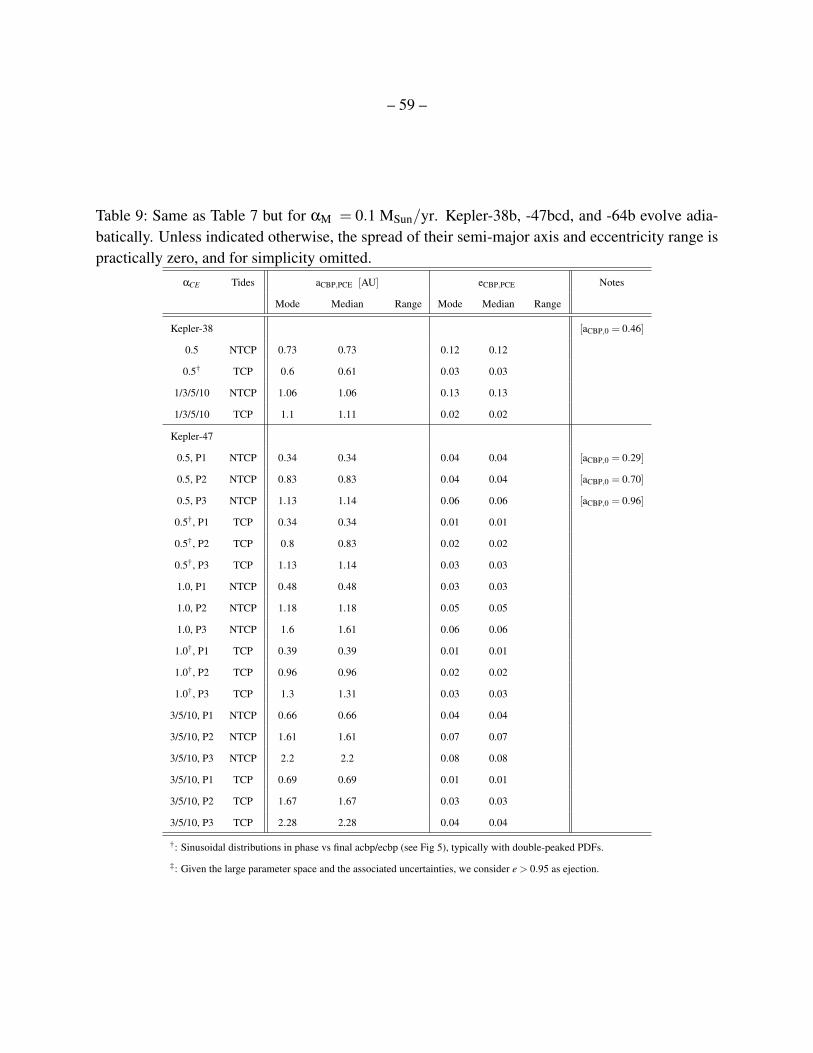
– 59 –

Table 9: Same as Table 7 but for αM = 0.1 MSun/yr. Kepler-38b, -47bcd, and -64b evolve adia-batically. Unless indicated otherwise, the spread of their semi-major axis and eccentricity range ispractically zero, and for simplicity omitted.

αCE Tides aCBP,PCE [AU] eCBP,PCE Notes

Mode Median Range Mode Median Range

Kepler-38 [aCBP,0 = 0.46]

0.5 NTCP 0.73 0.73 0.12 0.12

0.5† TCP 0.6 0.61 0.03 0.03

1/3/5/10 NTCP 1.06 1.06 0.13 0.13

1/3/5/10 TCP 1.1 1.11 0.02 0.02

Kepler-47

0.5, P1 NTCP 0.34 0.34 0.04 0.04 [aCBP,0 = 0.29]

0.5, P2 NTCP 0.83 0.83 0.04 0.04 [aCBP,0 = 0.70]

0.5, P3 NTCP 1.13 1.14 0.06 0.06 [aCBP,0 = 0.96]

0.5†, P1 TCP 0.34 0.34 0.01 0.01

0.5†, P2 TCP 0.8 0.83 0.02 0.02

0.5†, P3 TCP 1.13 1.14 0.03 0.03

1.0, P1 NTCP 0.48 0.48 0.03 0.03

1.0, P2 NTCP 1.18 1.18 0.05 0.05

1.0, P3 NTCP 1.6 1.61 0.06 0.06

1.0†, P1 TCP 0.39 0.39 0.01 0.01

1.0†, P2 TCP 0.96 0.96 0.02 0.02

1.0†, P3 TCP 1.3 1.31 0.03 0.03

3/5/10, P1 NTCP 0.66 0.66 0.04 0.04

3/5/10, P2 NTCP 1.61 1.61 0.07 0.07

3/5/10, P3 NTCP 2.2 2.2 0.08 0.08

3/5/10, P1 TCP 0.69 0.69 0.01 0.01

3/5/10, P2 TCP 1.67 1.67 0.03 0.03

3/5/10, P3 TCP 2.28 2.28 0.04 0.04

†: Sinusoidal distributions in phase vs final acbp/ecbp (see Fig 5), typically with double-peaked PDFs.

‡: Given the large parameter space and the associated uncertainties, we consider e > 0.95 as ejection.

– 60 –

Table 10: Same as Table 9.αCE Tides aCBP,PCE [AU] eCBP,PCE Notes

Mode Median Range Mode Median Range

Kepler-64 [aCBP,0 = 0.65]

0.5 NTCP 0.82 0.82 0.25 0.25 0.22–0.27

0.5† TCP 0.72 0.72 0.02 0.02

1.0 NTCP 1.58 1.58 0.31 0.33 0.31–0.35

1.0† TCP 0.91 0.91 0.01 0.01

3/5/10 NTCP 1.83 1.83 0.3 0.35 0.31–0.39

3/5/10 TCP 1.9 1.9 0.02 0.02

Kepler-1647§ [aCBP,0 = 2.71]

0.5 NTCP 2.52+1.53−0.01 3.55 2.33–40.61 0.7+0.02

−0.08 0.71 0.62–0.95‡ 27% ejected

0.5† TCP 3.1+0.19−0.01 3.19 3.08–3.3 0.11+0.01

−0.08 0.07 0.02–0.12

1.0 NTCP 3.91+0.67−0.01 4.45 3.83–20.27 0.72+0.22

−0.01 0.81 0.71–0.95 27% ejected

1.0† TCP 4.1 4.1 0.07 0.07

3/5/10 NTCP 4.7+0.63−0.26 4.93 4.29–19.14 0.7+0.19

−0.01 0.76 0.57–0.95 4% ejected

3/5/10 TCP 4.93 4.93 0.08 0.08

Kepler-1647§§

5.0†† NTCP 7.9+6.3−0.7 9.9 7.2–55.9 0.48+0.9

−0.1 0.55 0.2–0.95 82% ejected

10.0†† NTCP 7.7+4.0−0.8 9.2 6.9–31.1 0.32+0.25

−0.08 0.54 0.24–0.95 81% ejected

10.0 TCP – – – – – – 100% ejected

Kepler-35? [aCBP,0 = 0.60]

0.5 NTCP 0.94 0.94 0.37 0.37 0.33–0.41

0.5† TCP 0.95 0.95 0.03 0.03

1/3/5/10 NTCP 0.94 0.94 0.27 0.27 0.18–0.39

1/3/5/10 TCP 0.95 0.95 0.02 0.02

‡: Given the large parameter space and the associated uncertainties, we consider e > 0.95 as ejection.

§: Primary RLOF and CE.

§§: Secondary RLOF and CE.

?: Experiences CE for Z−1σZ.

††: Non-normal PDF with multiple peaks of comparable strength, mode not well defined.

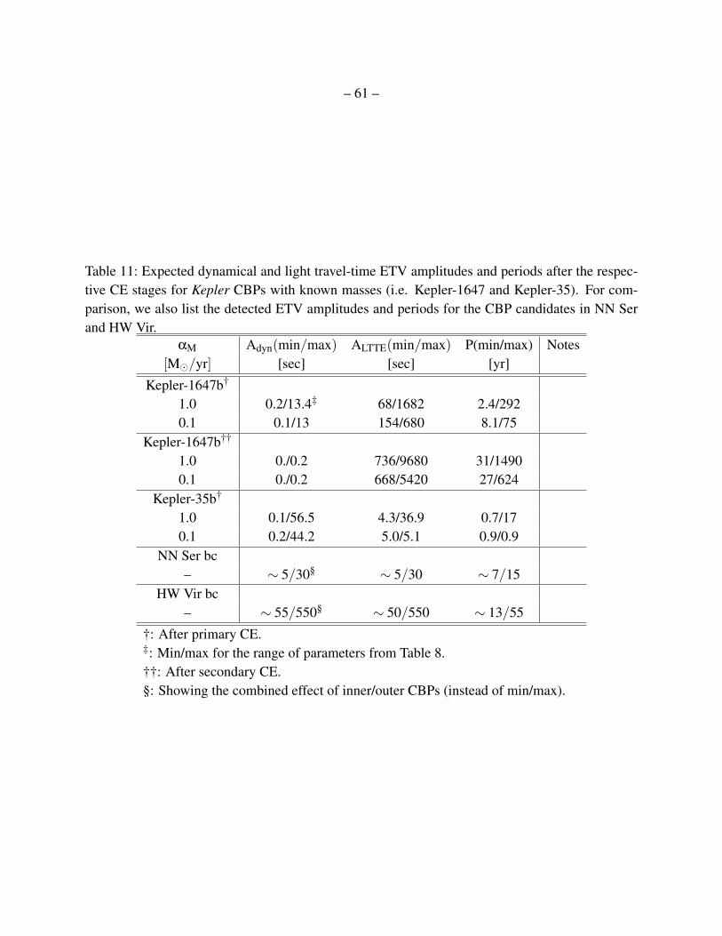
– 61 –

Table 11: Expected dynamical and light travel-time ETV amplitudes and periods after the respec-tive CE stages for Kepler CBPs with known masses (i.e. Kepler-1647 and Kepler-35). For com-parison, we also list the detected ETV amplitudes and periods for the CBP candidates in NN Serand HW Vir.

αM Adyn(min/max) ALTTE(min/max) P(min/max) Notes[M�/yr] [sec] [sec] [yr]

Kepler-1647b†

1.0 0.2/13.4‡ 68/1682 2.4/2920.1 0.1/13 154/680 8.1/75

Kepler-1647b††

1.0 0./0.2 736/9680 31/14900.1 0./0.2 668/5420 27/624

Kepler-35b†

1.0 0.1/56.5 4.3/36.9 0.7/170.1 0.2/44.2 5.0/5.1 0.9/0.9

NN Ser bc– ∼ 5/30§ ∼ 5/30 ∼ 7/15

HW Vir bc– ∼ 55/550§ ∼ 50/550 ∼ 13/55

†: After primary CE.‡: Min/max for the range of parameters from Table 8.††: After secondary CE.§: Showing the combined effect of inner/outer CBPs (instead of min/max).