Astronomy & Astrophysics manuscript no. planck˙boosting c© ESO 2013March 20, 2013

Planck 2013 results. XXVII. Doppler boosting of the CMB:Eppur si muove?

Planck Collaboration: N. Aghanim52, C. Armitage-Caplan81, M. Arnaud65, M. Ashdown62,5, F. Atrio-Barandela15, J. Aumont52, A. J. Banday83,8,R. B. Barreiro59, J. G. Bartlett1,60, K. Benabed53,82, A. Benoit-Levy21,53,82, J.-P. Bernard8, M. Bersanelli32,44, P. Bielewicz83,8,75, J. Bobin65,

J. J. Bock60,9, J. R. Bond7, J. Borrill11,79, F. R. Bouchet53,82, M. Bridges62,5,56, C. Burigana43,30, R. C. Butler43, J.-F. Cardoso66,1,53, A. Catalano67,64,A. Challinor56,62,10, A. Chamballu65,12,52, L.-Y Chiang55, H. C. Chiang24,6, P. R. Christensen72,35, D. L. Clements50, L. P. L. Colombo20,60,

F. Couchot63, B. P. Crill60,73, F. Cuttaia43, L. Danese75, R. D. Davies61, R. J. Davis61, P. de Bernardis31, A. de Rosa43, G. de Zotti40,75,J. Delabrouille1, J. M. Diego59, S. Donzelli44, O. Dore60,9, X. Dupac37, G. Efstathiou56, T. A. Enßlin70, H. K. Eriksen57, F. Finelli43,45, O. Forni83,8,

M. Frailis42, E. Franceschi43, S. Galeotta42, K. Ganga1, M. Giard83,8, G. Giardino38, J. Gonzalez-Nuevo59,75, K. M. Gorski60,86, S. Gratton62,56,A. Gregorio33,42, A. Gruppuso43, F. K. Hansen57, D. Hanson71,60,7, D. Harrison56,62, G. Helou9, S. R. Hildebrandt9, E. Hivon53,82, M. Hobson5,W. A. Holmes60, W. Hovest70, K. M. Huffenberger85, W. C. Jones24, M. Juvela23, E. Keihanen23, R. Keskitalo18,11, T. S. Kisner69, J. Knoche70,

L. Knox26, M. Kunz14,52,3, H. Kurki-Suonio23,39, A. Lahteenmaki2,39, J.-M. Lamarre64, A. Lasenby5,62, C. R. Lawrence60, R. Leonardi37,A. Lewis22, M. Liguori29, P. B. Lilje57, M. Linden-Vørnle13, M. Lopez-Caniego59, P. M. Lubin27, J. F. Macıas-Perez67, M. Maris42,

D. J. Marshall65, P. G. Martin7, E. Martınez-Gonzalez59, S. Masi31, S. Matarrese29, P. Mazzotta34, P. R. Meinhold27, A. Melchiorri31,46,L. Mendes37, M. Migliaccio56,62, S. Mitra49,60, A. Moneti53, L. Montier83,8, G. Morgante43, D. Mortlock50, A. Moss77, D. Munshi76,

P. Naselsky72,35, F. Nati31, P. Natoli30,4,43, H. U. Nørgaard-Nielsen13, F. Noviello61, D. Novikov50, I. Novikov72, S. Osborne80, C. A. Oxborrow13,L. Pagano31,46, F. Pajot52, D. Paoletti43,45, F. Pasian42, G. Patanchon1, O. Perdereau63, F. Perrotta75, F. Piacentini31, E. Pierpaoli20, D. Pietrobon60,S. Plaszczynski63, E. Pointecouteau83,8, G. Polenta4,41, N. Ponthieu52,47, L. Popa54, G. W. Pratt65, G. Prezeau9,60, J.-L. Puget52, J. P. Rachen17,70,W. T. Reach84, M. Reinecke70, S. Ricciardi43, T. Riller70, I. Ristorcelli83,8, G. Rocha60,9, C. Rosset1, J. A. Rubino-Martın58,36, B. Rusholme51,

D. Santos67, G. Savini74, D. Scott19??, M. D. Seiffert60,9, E. P. S. Shellard10, L. D. Spencer76, R. Sunyaev70,78, F. Sureau65, A.-S. Suur-Uski23,39,J.-F. Sygnet53, J. A. Tauber38, D. Tavagnacco42,33, L. Terenzi43, L. Toffolatti16,59, M. Tomasi44, M. Tristram63, M. Tucci14,63, M. Turler48,

L. Valenziano43, J. Valiviita39,23,57, B. Van Tent68, P. Vielva59, F. Villa43, N. Vittorio34, L. A. Wade60, B. D. Wandelt53,82,28, M. White25, D. Yvon12,A. Zacchei42, J. P. Zibin19, and A. Zonca27

Preprint online version: 20 March 2013

ABSTRACT

Our velocity relative to the rest frame of the cosmic microwave background (CMB) generates a dipole temperature anisotropy on thesky which has been well measured for more than 30 years, and has an accepted amplitude of v/c = 1.23 × 10−3, or v = 369 km s−1.In addition to this signal generated by Doppler boosting of the CMB monopole, our motion also modulates and aberrates the CMBtemperature fluctuations (as well as every other source of radiation at cosmological distances). This is an order 10−3 effect appliedto fluctuations which are already one part in roughly 10−5, so it is quite small. Nevertheless, it becomes detectable with the all-skycoverage, high angular resolution, and low noise levels of the Planck satellite. Here we report a first measurement of this velocitysignature using the aberration and modulation effects on the CMB temperature anisotropies, finding a component in the known dipoledirection, (l, b) = (264◦, 48◦), of 384 km s−1 ± 78 km s−1 (stat.) ± 115 km s−1 (syst.). This is a significant confirmation of the expectedvelocity.

Key words. Cosmology: observations – cosmic background radiation – Reference systems – Relativistic processes

1. Introduction

This paper, one of a set associated with the 2013 release ofdata from the Planck† mission (Planck Collaboration I 2013),presents a study of Doppler boosting effects using the small scaletemperature fluctuations of the Planck CMB maps.

? “And yet it moves,” the phrase popularly attributed to GalileoGalilei after being forced to recant his view that the Earth goes aroundthe Sun.?? Corresponding author: D. Scott <dscott@phas.ubc.ca>† Planck (http://www.esa.int/Planck) is a project of the

European Space Agency (ESA) with instruments provided by two sci-entific consortia funded by ESA member states (in particular the leadcountries France and Italy), with contributions from NASA (USA) andtelescope reflectors provided by a collaboration between ESA and a sci-entific consortium led and funded by Denmark.

Observations of the large cosmic microwave background(CMB) temperature dipole are usually taken to indicate that ourSolar System barycentre is in motion with respect to the CMBframe (defined precisely below). Assuming that the observedtemperature dipole is due entirely to Doppler boosting of theCMB monopole, one infers a velocity v = (369 ± 0.9) km s−1 inthe direction (l, b) = (263.99◦ ± 0.14◦, 48.26◦ ± 0.03◦), on theboundary of the constellations of Crater and Leo (Kogut et al.1993; Fixsen et al. 1996; Hinshaw et al. 2009).

In addition to Doppler boosting of the CMB monopole, ve-locity effects also boost the order 10−5 primordial temperaturefluctuations. There are two observable effects here, both at alevel of β ≡ v/c = 1.23 × 10−3. First, there is a Doppler “modu-lation” effect, which amplifies the apparent temperature fluctua-tions in the velocity direction. This is the same effect which con-verts a portion of the CMB monopole into the observed dipole.

1

Planck Collaboration: Doppler boosting of the CMB: Eppur si muove

The effect on the CMB fluctuations is to increase the amplitudeof the power spectrum by approximately 0.25% in the velocitydirection, and decrease it correspondingly in the anti-direction.Second, there is an “aberration” effect, in which the apparent ar-rival direction of CMB photons is pushed toward the velocitydirection. This effect is small, but non-negligible. The expectedvelocity induces a peak deflection of β = 4.2′ and a root-mean-squared (rms) deflection over the sky of 3′, comparable to theeffects of gravitational lensing by large-scale structure, whichare discussed in Planck Collaboration XVII (2013). The aber-ration effect squashes the anisotropy pattern on one side of thesky and stretches it on the other, effectively changing the angu-lar scale. Close to the velocity direction we expect that the powerspectrum of the temperature anisotropies, C`, will be shifted sothat, e.g., `= 1000→ `= 1001, while `= 1000→ `= 999 in theanti-direction. In Fig. 1 we plot an exaggerated illustration of theaberration and modulation effects. For completeness we shouldpoint out that there is a third effect, a quadrupole of amplitudeβ2 induced by the dipole (see Kamionkowski & Knox 2003).However, extracting this signal would require extreme levels ofprecision for foreground modelling at the quadrupole scale, andwe do not discuss it further.

In this paper, we will present a measurement of β, exploitingthe distinctive statistical signatures of the aberration and mod-ulation effects on the high-` CMB temperature anisotropies. Inaddition to our interest in making an independent measurementof the velocity signature, the effects which velocity generates onthe CMB fluctuations provide a source of potential bias or con-fusion for several aspects of the Planck data. In particular, ve-locity effects couple to measurements of: primordial “τNL”-typenon-Gaussianity, as discussed in Planck Collaboration XXIV(2013); statistical anisotropy of the primordial CMB fluctua-tions, as discussed in Planck Collaboration XXIII (2013); andgravitational lensing, as discussed in Planck Collaboration XVII(2013). There are also aspects of the Planck analysis for whichvelocity effects are believed to be negligible, but only if they arepresent at the expected level. One example is measurement offNL-type non-Gaussianity, as discussed in Catena et al. (2013).Another example is power spectrum estimation; as discussedabove, velocity effects change the angular scale of the acous-tic peaks in the CMB power spectrum. Averaged over the fullsky this effect is strongly suppressed, as the expansion and con-traction of scales on opposing hemispheres cancel out. Howeverthe application of a sky mask breaks this cancellation to someextent, and can potentially be important for parameter estima-tion (Pereira et al. 2010; Catena & Notari 2012). For the 143and 217 GHz analysis mask used in the fiducial Planck CMBlikelihood (Planck Collaboration XV 2013), the average lensingconvergence field associated with the aberration effect (on theportion of the sky which is unmasked) has a value which is 13%of its peak value, corresponding to an expected average lensingconvergence of β× 0.13 = 1.5× 10−4. This will shift the angularscale of the acoustic peaks by the same fraction, which is de-generate with a change in the angular size of the sound horizonat last scattering, θ∗ (Burles & Rappaport 2006). A 1.5 × 10−4

shift in θ∗ is just under 25% of the Planck uncertainty on this pa-rameter, as reported in Planck Collaboration XVI (2013)—smallenough to be neglected, though not dramatically so. Therefore itdoes motivate us to test that the observed aberration signal is notsignificantly larger than expected. With such a confirmation inhand, a logical next step is to correct for these effects by a pro-cess of de-boosting the observed temperature Notari & Quartin(2012); Yoho et al. (2012).

(a) T primordial

(b) Taberration

(c) Tmodulation

Fig. 1. Exaggerated illustration of the Doppler aberration andmodulation effects, in orthographic projection, for a velocityv = 260 000 km s−1 = 0.85c (approximately 700 times largerthan the expected magnitude) toward the northern pole (indi-cated by meridians in the upper half of each image on the left).The aberration component of the effect shifts the apparent posi-tion of fluctuations toward the velocity direction, while the mod-ulation component enhances the fluctuations in the velocity di-rection and suppresses them in the anti-velocity direction.

Before proceeding to discuss the aberration and modulationeffects in more detail, we note that in addition to the overall pe-culiar velocity of our Solar System with respect to the CMB,there is an additional time-dependent velocity effect from the or-bit of Planck (at L2, along with the Earth) about the Sun. Thisvelocity has an average amplitude of approximately 30 km s−1,less than one-tenth the size of the primary velocity effect. Theaberration component of the orbital velocity (more commonlyreferred to in astronomy as “stellar aberration”) has a maximumamplitude of 21′′ and is corrected for in the satellite pointing.The modulation effect for the orbital velocity switches signs be-tween each 6-month survey, and so is suppressed when usingmultiple surveys to make maps (as we do here, with the nominalPlanck maps, based on a little more than two surveys), and sowe will not consider it further here.

2. Aberration and modulation

Here we will present a more quantitative description of the aber-ration and modulation effects described above. To begin, notethat, by construction, the peculiar velocity, β, measures the ve-

2

Planck Collaboration: Doppler boosting of the CMB: Eppur si muove

locity of our Solar System barycentre relative to a frame, calledthe CMB frame, in which the temperature dipole, a1m, vanishes.However, in completely subtracting the dipole, this frame wouldnot coincide with a suitably-defined average CMB frame, inwhich an observer would expect to see a dipole C1 ∼ 10−10,given by the Sachs-Wolfe and integrated Sachs-Wolfe effects.The velocity difference between these two frames is, however,small, at the level of 1% of our observed v.

If T ′ and n ′ are the CMB temperature and direction asviewed in the CMB frame, then the temperature in the observedframe is given by the Lorentz transformation (see, e.g., Challinor& van Leeuwen 2002; Sollom 2010),

T (n ) =T ′(n ′)

γ(1 − n · β), (1)

where the observed direction n is given by

n =n ′ + [(γ − 1)n ′ · v + γβ]v

γ(1 + n ′ · β), (2)

and γ ≡ (1 − β2)−1/2. Expanding to linear order in β gives

T ′(n ′) = T ′(n − ∇(n · β)) ≡ T0 + δT ′(n − ∇(n · β)), (3)

so that we can write the observed temperature fluctuations as

δT (n ) = T0 n · β + δT ′(n − ∇(n · β))(1 + n · β). (4)

Here T0 = (2.7255 ± 0.0006) K is the CMB mean temperature(Fixsen 2009). The first term on the right-hand side of Eq. (4) isthe temperature dipole. The remaining term represents the fluc-tuations, aberrated by deflection ∇(n · β) and modulated by thefactor (1 + n · β).

The Planck detectors can be modelled as measuring differ-ential changes in the CMB intensity at frequency ν given by

Iν(ν, n ) =2hν3

c2

1exp [hν/kBT (n )] − 1

. (5)

We can expand the measured intensity difference according to

δIν(ν, n ) =dIνdT

∣∣∣∣∣T0

δT (n ) +12

d2IνdT 2

∣∣∣∣∣∣T0

δT 2(n ) + . . . . (6)

Substituting Eq. (4) and dropping terms of order (β2) and (δT 2),we find

δIν(ν, n ) =dIνdT

∣∣∣∣∣T0

(T0 n · β + δT ′(n ′)(1 + bν n · β)

), (7)

where the frequency dependent boost factor bν is given by

bν =ν

ν0coth

(ν

2ν0

)− 1, (8)

with ν0 ≡ kBT0/h ' 57 GHz. Integrated over the Planck band-passes for the 143 and 217 GHz channels, these effective boostfactors are given by b143 = 1.961 ± 0.015, and b217 = 3.071 ±0.018, where the uncertainties give the scatter between the indi-vidual detector bandpasses at each frequency. We will approxi-mate these boost factors simply as b143 = 2 and b217 = 3, whichis sufficiently accurate for the precision of our measurement.

The inferred temperature fluctuations will then be

δIν(ν, n )dIν/dT |T0

= T0 n · β + δT ′(n − ∇(n · β))(1 + bν n · β). (9)

+ ~β

−~β + ~β

− ~β

+ ~β×− ~β×

Fig. 2. Decomposition of the dipole vector β in Galactic co-ordinates. The CMB dipole direction (l, b) = (263.99◦, 48.26◦)is given as β‖, while two directions orthogonal to it (and eachother) are denoted as β⊥ and β×. The vector β× lies within theGalactic plane.

Notice that, compared with the actual fluctuations in Eq. (4), themodulation term in Eq. (9) has taken on a peculiar frequency de-pendence, represented by bν. This has arisen due to the couplingbetween the fluctuations and the dipole, T0 n · β, which leadsto a second-order term in the expansion of Eq. (6). Intuitively,the CMB temperature varies from one side of the sky to theother at the 3 mK level. Therefore so does the calibration factordIν/dT , as represented by the second derivative d2Iν/dT 2. Wenote that such a frequency dependent modulation is not uniquelya velocity effect, but would have arisen in the presence of anysufficiently large temperature fluctuation. Of course if we mea-sured T (n ) directly (for example by measuring Iν(ν, n ) at a largenumber of frequencies), we would measure the true fluctuations,Eq. (4) (i.e., we would have a boost factor of bν = 1).

3. Methodology

The statistical properties of the aberration-induced stretchingand compression of the CMB anisotropies are manifest in “sta-tistically anisotropic” contributions to the covariance matrix ofthe CMB, which we can use to reconstruct the velocity vec-tor (Burles & Rappaport 2006; Kosowsky & Kahniashvili 2011;Amendola et al. 2011). To discuss these it will be useful to in-troduce the harmonic transform of the peculiar velocity vector,given by

βLM =

∫dn Y∗LM(n )β · n . (10)

Here βLM is only non-zero for dipole modes (with L = 1).Although most of our equations will be written in terms of βLM ,for simplicity of interpretation we will present results in a spe-cific choice of basis for the three dipole modes of orthonormalunit vectors, labelled β‖ (along the expected velocity direction),β× (perpendicular to β‖ and parallel to the Galactic plane, nearits centre), and the remaining perpendicular mode β⊥. The direc-tions associated with these modes are plotted in Fig. 2.

In the statistics of the CMB fluctuations, peculiar velocityeffects manifest themselves as a set of off-diagonal contributionsto the CMB covariance matrix:

〈T`1m2 T`2m2〉cmb =∑LM

(−1)M(`1 `2 Lm1 m2 M

)

×

√(2`1 + 1)(2`2 + 1)(2L + 1)

4πWβν`1`2L βLM , (11)

3

Planck Collaboration: Doppler boosting of the CMB: Eppur si muove

where the weight function Wβν is composed of two parts, relatedto the aberration and modulation effects, respectively:

Wβν`1`2L = Wφ

`1`2L + bνWτ`1`2L. (12)

The aberration term is identical to that found when consideringgravitational lensing of the CMB by large scale structure (Lewis& Challinor 2006; Planck Collaboration XVII 2013),

Wφ`1`2L = −

(1 + (−1)`1+`2+L

2

) √L(L + 1)`1(`1 + 1)

×CTT`1

(`1 `2 L1 0 −1

)+ (`1 ↔ `2), (13)

while the modulation term is identical to that produced byan inhomogeneous optical depth to the last scattering surface(Dvorkin & Smith 2009),

Wτ`1`2L =

(`1 `2 L0 0 0

) (CTT`1

+ CTT`2

). (14)

Note that one might in principle be concerned about order β2

corrections to the covariance matrix, particularly at high ` (see,e.g., Notari & Quartin 2012). However, these are small, providedthat the spectra are relatively smooth. Although the order β ('10−3) deflections give large changes to the a`ms for ` > 103, thechanges to the overall covariance are small (Chluba 2011), sincethe deflection effect is coherent over very large scales.

Note that these boosting-induced correlations couple ` with` ± 1 modes. They therefore share this property with pure dipo-lar amplitude modulations studied in the context of primordialstatistical anisotropy (see, e.g, Prunet et al. 2005), as well aswith dipolar modulations in more general physical parameters(Moss et al. 2011). However, these other cases do not share thefrequency dependence of the boosting modulation effect, sincethey are not accompanied by a temperature dipole.

We measure the peculiar velocity dipole using quadratic es-timators, essentially summing over the covariance matrix of theobserved CMB fluctuations, with weights designed to optimallyextract β. A general quadratic estimator x for β is given by(Hanson & Lewis 2009)

xLM[T ] =12

N xβνL

`max∑`1=`min

`max∑`2=`min

∑m1,m2

(−1)M(`1 `2 Lm1 m2 −M

)W x`1`2L

×(T`1m1

T`2m2− 〈T`1m1

T`2m2〉), (15)

where T`m are a set of inverse-variance filtered temperature mul-tipoles, W x

`1`2L is a weight function and N xβνL is a normalization.

The ensemble average term 〈〉 is taken over signal+noise real-izations of the CMB in the absence of velocity effects. It cor-rects for the statistical anisotropy induced by effects like beamasymmetry, masking, and noise inhomogeneity. We evaluate thisterm using Monte Carlo simulations of the data, as discussed inSect. 4.

We use three different quadratic estimators to measure the ef-fect of boosting. The first, β, simply adopts the weight functionWβν`1`2L, and provides a minimum-variance estimator of the to-

tal peculiar velocity effect. The two additional estimators, φ andτ, isolate the aberration and modulation aspects of the peculiarvelocity effect, respectively. This can be useful, as they are qual-itatively quite distinct effects, and suffer from different potentialcontaminants. The modulation effect, for example, is degenerate

with a dipolar pattern of calibration errors on the sky, while theaberration effect is indistinguishable from a dipolar pattern ofpointing errors.

There is a subtlety in the construction of these estimators,due to the fact that the covariances described by Wφ and Wτ arenot orthogonal. To truly isolate the aberration and modulationeffects, we form orthogonalized weight matrices as

W φ`1`2L = Wφ

`1`2L −Wτ`1`2LR

φτL /R

ττL and (16)

W τ`1`2L = Wτ

`1`2L −Wφ`1`2LR

τφL /R

φφL , (17)

where the response function R is given by

RxzL =

1(2L + 1)

`max∑`1=`min

`max∑`2=`min

12

W x`1`2LWz

`1`2LF`1F`2

, (18)

with x, z = βν, φ, τ. The construction of these estimators is analo-gous to the construction of “bias-hardened” estimators for CMBlensing (Namikawa et al. 2012). The spectra F` are diagonal ap-proximations to the inverse variance filter, which takes the skymap T → T . We use the same inverse variance filter as that usedfor the baseline results in Planck Collaboration XVII (2013), andthe approximate filter functions are also specified there. Notethat our φ estimator is slightly different from that used in PlanckCollaboration XVII (2013), due to the fact that we have orthog-onalized it with respect to τ.

The normalization N xβνL can be approximated analytically as

N xβνL '

[R

xβνL

]−1. (19)

This approximation does not account for masking. On a maskedsky, with this normalization, we expect to find that 〈xLM〉 =fLM,skyβLM , where

fLM,sky =

∫dn Y∗LM(n )M(n )β‖ · n . (20)

Here M(n ) is the sky mask used in our analysis. For the fidu-cial sky mask we use (plotted in Fig. 2, which leaves approx-imately 70% of the sky unmasked), rotating fLM,sky onto ourthree basis vectors we find that f‖, sky = 0.82, f⊥, sky = 0.17and f×, sky = −0.04. The large effective sky fraction for the β‖direction reflects the fact that the peaks of the expected velocitydipole are untouched by the mask, while the small values of fskyfor the other components reflects that fact that the masking pro-cedure does not leak a large amount of the dipole signal in theβ‖ direction into other modes.

4. Data and simulations

Given the frequency-dependent nature of the velocity effects weare searching for (at least for the τ component), we will focusfor the most part on estimates of β obtained from individual fre-quency maps, although in Sect. 6 we will also discuss the analy-sis of component-separated maps obtained from combinations ofthe entire Planck frequency range. Our analysis procedure is es-sentially identical to that of Planck Collaboration XVII (2013),and so we only provide a brief review of it here. We use the143 and 217 GHz Planck maps, which contain the majority ofthe available CMB signal probed by Planck at the high mul-tipoles required to observe the velocity effects. The 143 GHzmap has a noise level that is reasonably well approximated by

4

Planck Collaboration: Doppler boosting of the CMB: Eppur si muove

45 µK arcmin white noise, while the 217 GHz map has approx-imately twice as much power, with a level of 60 µK arcmin.The beam at 143 GHz is approximately 7′ FWHM, while the217 GHz beam is 5′ FWHM. This increased angular resolu-tion, as well as the larger size of the τ-type velocity signal athigher frequency, makes 217 GHz slightly more powerful than143 GHz for detecting velocity effects (the HFI 100 GHz and LFI70 GHz channels would offer very little additional constrainingpower). At these noise levels, for 70% sky coverage we Fisher-forecast a 20% measurement of the component β‖ at 217 GHz(or, alternatively, a 5σ detection) or a 25% measurement ofβ‖ at 143 GHz, consistent with the estimates of Kosowsky &Kahniashvili (2011). As we will see, our actual statistical errorbars determined from simulations agree well with these expec-tations.

The Planck maps are generated at HEALPix (Gorski et al.2005)‡ Nside = 2048. In the process of mapmaking, time-domainobservations are binned into pixels. This effectively generates apointing error, given by the distance between the pixel centre towhich each observation is assigned and the true pointing direc-tion at that time. The pixels at Nside = 2048 have a typical dimen-sion of 1.7′. As this is comparable to the size of the aberrationeffect we are looking for, this is a potential source of concern.However, as discussed in Planck Collaboration XVII (2013), thebeam-convolved CMB is sufficiently smooth on these scales thatit is well approximated as a gradient across each pixel, and theerrors accordingly average down with the distribution of hits ineach pixel. For the frequency maps that we use, the rms pix-elization error is on the order of 0.1′, and not coherent over thelarge dipole scales which we are interested in, and so we neglectpixelization effects in our measurement.

We will use several data combinations to measure β. Thequadratic estimator of Eq. (15) has two input “legs,” i.e., the `1m1and `2m2 terms. Starting from the 143 and 217 GHz maps, thereare three distinct ways we may source these legs: (1) both legsuse either the individually filtered 143 GHz or 217 GHz maps,which we refer to as 143 × 143 and 217 × 217, respectively; (2)we can use 143 GHz for one leg, and 217 GHz for the other, re-ferred to as 143 × 217; and (3) we can combine both 143 and217 GHz data in our inverse-variance filtering procedure intoa single minimum-variance map, which is then fed into bothlegs of the quadratic estimator. We refer to this final combina-tion schematically as “143+217.” Combinations (2) and (3) mix143 and 217 GHz data. When constructing the weight functionof Eq. (12) for these combinations we use an effective bν = 2.5.To construct the T , which are the inputs for these quadratic esti-mators, we use the filtering described in Appendix A of PlanckCollaboration XVII (2013), which optimally accounts for theGalactic and point source masking (although not for the inho-mogeneity of the instrumental noise level). This filter inverse-variance weights the CMB fluctuations, and also projects out the857 GHz Planck map as a dust template.

To characterize our estimator and to compute the mean-fieldterm of Eq. (15), we use a large set of Monte Carlo simula-tions. These are generated following the same procedure as thosedescribed in Planck Collaboration XVII (2013); they incorpo-rate the asymmetry of the instrumental beam, gravitational lens-ing effects, and realistic noise realizations from the FFP6 sim-ulation set described in Planck Collaboration I (2013). Thereis one missing aspect of these simulations which we discussbriefly here: due to an oversight in their preparation, the gravita-tional lensing component of our simulations only included lens-

‡ http://healpix.jpl.nasa.gov

ing power for lensing modes on scales L ≥ 2, which leads to aslight underestimation of our simulation-based error bars for theφ component of the velocity estimator. The lensing dipole powerin the fiducial ΛCDM model is Cφφ

1 ' 6 × 10−8, which repre-sents an additional source of noise for each mode of β, givenby σφ,lens = 1.2 × 10−4, or about one tenth the size of the ex-pected signal. The φ part of the estimator contributes approx-imately 46% of the total β estimator weight at 143 GHz, and35% at 217 GHz. Our measurement errors without this lensingnoise on an individual mode of β are σβ ' 2.5 × 10−4, whilewith lensing noise included we would expect this to increase to√σ2β + (4/10)2σ2

φ,lens = 2.54 × 10−4. This is small enough thatwe have neglected it for these results (rather than include it byhand).

We generate simulations both with and without peculiar ve-locity effects, to determine the normalization of our estimator,which, as we will see, is reasonably consistent with the analyt-ical expectation discussed around Eq. (20). All of our main re-sults with frequency maps use 1000 simulations to determine theestimator mean field and variance, while the component separa-tion tests in Sect. 6 use 300 simulations.

5. Results

We introduce our results visually in Fig. 3, where we plot thetotal measured dipole direction β as a function of the maximumtemperature multipole `max used as input to our quadratic estima-tors. We can see that all four of our 143/217 GHz based estima-tors converge toward the expected dipole direction at high `max.At `max < 100, we recover the significantly preferred directionof Hoftuft et al. (2009), which is identified when searching for adipolar modulation of the CMB fluctuations. The τ componentof the velocity effect is degenerate with such a modulation (atleast at fixed frequency), and φ gets little weight from ` < 100,so this is an expected result. The significance of this preferred di-rection varies as a function of smoothing scale (Hanson & Lewis2009; Bennett et al. 2011; Planck Collaboration XXIII 2013).To minimize possible contamination on our results by this po-tential anomaly, from here onward we restrict the temperaturemultipoles used in our β estimation to `min = 500. This cut re-moves only about 10% of the total number of modes measuredby Planck, and so does not significantly increase our error bars.

There is a clear tendency in Fig. 3 for the measured velocityto point toward the expected direction β‖. At Planck noise levels,we expect a one standard-deviation uncertainty on each compo-nent of β of better than 25%. A 25% uncertainty corresponds toan arctan(1/4) = 14◦ constraint on the direction of β. We plotthis contour, as well as the corresponding two standard devia-tion contour arctan(2/4) = 26◦. It is apparent that the measuredvelocity directions are in reasonable agreement with the CMBdipole.

We now proceed to break the measurement of Fig. 3 intoits constituent parts for `max = 2000 (and truncating now at`min = 500). In Fig. 4 we plot our quadratic estimates of thethree components of β, as well as the decomposition into aberra-tion and modulation components for each of our four frequencycombinations. The vertical lines in Fig. 4 give the amplitude es-timates for each component measured from the data, while thecoloured and grey histograms give the distribution of these quan-tities for the 143×217 estimator for simulations with and withoutvelocity effects, respectively (the other estimators are similar).As expected, the velocity effects show up primarily in β‖; thereis little leakage into other components with our sky mask. For all

5

Planck Collaboration: Doppler boosting of the CMB: Eppur si muove

100 2000lmax

+ ~β

−~β

+ ~β

− ~β

+ ~β×− ~β×

Fig. 3. Measured dipole direction β in Galactic coordinates as a function of the maximum temperature multipole used in theanalysis, `max. We plot the results for the four data combinations discussed in Sect. 4: 143× 143 (H symbol); 217× 217 (N symbol);143 × 217 (× symbol); and 143 + 217 (+ symbol). The CMB dipole direction β‖ has been highlighted with 14◦ and 26◦ radiuscircles, which correspond roughly to our expected uncertainty on the dipole direction. The black cross in the lower hemisphere isthe modulation dipole anomaly direction found for WMAP at `max = 64 in Hoftuft et al. (2009), and which is discussed further inPlanck Collaboration XXIII (2013). Note that all four estimators are significantly correlated with one another, even the 143 × 143and 217 × 217 results, which are based on maps with independent noise realizations. This is because a significant portion of thedipole measurement uncertainty is from sample variance of the CMB fluctuations, which is common between channels.

four estimators, we see that the presence of velocity along β‖ isstrongly preferred over the null hypothesis. At 143 GHz this sig-nal comes from both φ‖ and τ‖. At 217 GHz it comes primarilyfrom τ‖. Additionally, there is a somewhat unexpected signal at217 GHz in the β× direction, again driven by the τ component.Given the apparent frequency dependence, foreground contami-nation seems a possible candidate for this anomalous signal. Wewill discuss this possibility further in the next section.

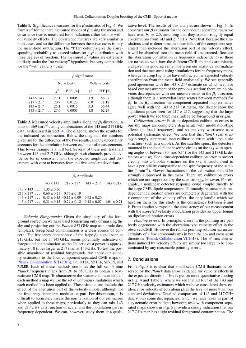
In Table 1 we present χ2 values for the β measurements ofFig. 4 under both the null hypothesis of no velocity effects, aswell as assuming the expected velocity direction and amplitude.We can see that all of our measurements are in significant dis-agreement with the “no velocity” hypothesis. The probability-to-exceed (PTE) values for the “with velocity” case are muchmore reasonable. Under the velocity hypothesis, 217 × 217 hasthe lowest PTE of 11%, driven by the large β×.

In Table 2 we focus on our measurements of the velocityamplitude along the expected direction β‖, as well as perform-ing null tests among our collection of estimates. For this table,we have normalized the estimators, such that the average of β‖on boosted simulations is equal to the input value of 369 km s−1.For all four of our estimators, we find that this normalizationfactor is within 0.5% of that given by N xβν f‖,sky, as is already ap-

parent from the triangles along the horizontal axis of Fig. 4. Wecan see here, as expected, that our estimators have a statisticaluncertainty on β‖ of between 20% and 25%. However, severalof our null tests, obtained by taking the differences of pairs of β‖estimates, fail at the level of two or three standard deviations. Wetake the 143 × 217 GHz estimator as our fiducial measurement;as it involves the cross-correlation of two maps with indepen-dent noise realizations it should be robust to noise modelling.Null tests against the individual 143 and 217 GHz estimates arein tension at a level of two standard deviations for this estima-tor. We take this tension as a measure of the systematic differ-ences between these two channels, and conservatively choosethe largest discrepancy with the 143×217 GHz estimate, namely0.31, as our systematic error. We therefore report a measurementof v‖ = 384 km s−1 ± 78 km s−1 (stat.) ± 115 km s−1 (syst.), a sig-nificant confirmation of the expected velocity amplitude.

6. Potential contaminants

There are several potential sources of contamination for our es-timates above which we discuss briefly here, although we havenot attempted an exhaustive study of potential contaminants forour estimator.

6

Planck Collaboration: Doppler boosting of the CMB: Eppur si muove

1.5 1.0 0.5 0.0 0.5 1.0 1.5

β

143× 143

217× 217

143 +143

143× 217

1.5 1.0 0.5 0.0 0.5 1.0 1.5

φ

1.5 1.0 0.5 0.0 0.5 1.0 1.5

τ

1.5 1.0 0.5 0.0 0.5 1.0 1.5

β

1.5 1.0 0.5 0.0 0.5 1.0 1.5

φ

1.5 1.0 0.5 0.0 0.5 1.0 1.5

τ

1.5 1.0 0.5 0.0 0.5 1.0 1.5

β×

1.5 1.0 0.5 0.0 0.5 1.0 1.5

φ×

1.5 1.0 0.5 0.0 0.5 1.0 1.5

τ×

Fig. 4. Measurements of β using combinations of the 143 and 217 GHz Planck maps, normalized using Eq. (19) and then dividedby the fiducial amplitude of β = 1.23 × 10−3. These estimates use `min = 500 and `max = 2000. In addition to the total minimumvariance estimate β, the measurement is also broken down into its aberration-type part, φ, and modulation-type part, τ. Vertical linesgive the Planck measurement for the four estimates described in the text. Grey histograms give the distribution of estimates forsimulations of the 143 × 217 estimator, which do not contain peculiar velocity effects (the other estimators are very similar). Thered histograms give the distribution for simulations which do contain peculiar velocity effects, simulated with the fiducial direction(along β‖) and amplitude. Black triangles on the x-axis indicate the relevant component of fsky given by Eq. (20), which agrees wellwith the peak of the velocity simulations.

1.5 1.0 0.5 0.0 0.5 1.0 1.5

β

NILC

SMICA

SEVEM

RULER

1.5 1.0 0.5 0.0 0.5 1.0 1.5

φ

1.5 1.0 0.5 0.0 0.5 1.0 1.5

τ

1.5 1.0 0.5 0.0 0.5 1.0 1.5

β

1.5 1.0 0.5 0.0 0.5 1.0 1.5

φ

1.5 1.0 0.5 0.0 0.5 1.0 1.5

τ

1.5 1.0 0.5 0.0 0.5 1.0 1.5

β×

1.5 1.0 0.5 0.0 0.5 1.0 1.5

φ×

1.5 1.0 0.5 0.0 0.5 1.0 1.5

τ×

Fig. 5. Plot of velocity amplitude estimates, similar to Fig. 4, but using an array of component-separated maps rather than specificcombinations of frequency maps. The production and characterization of these component separated maps is presented in PlanckCollaboration XII (2013). Histograms of simulation results without velocity effects are overplotted in grey for each method; theyare all very similar. Vertical coloured bars correspond to the maps indicated in the legend, using the combination of our fiducialgalaxy mask (which removes approximately 30% of the sky) as well as the specific mask produced for each component separationmethod. We see significant departures from the null-hypothesis simulations only in the β‖ direction, as expected. Vertical black linesshow the 143× 217 measurement of Fig. 4. Please note the discussion about the subtleties in the normalization of these estimates inSect. 6. 7

Planck Collaboration: Doppler boosting of the CMB: Eppur si muove

Table 1. Significance measures for the β estimates of Fig. 4. Weform a χ2 for the three measured modes of β, using the mean andcovariance matrix measured for simulations either with or with-out velocity effects. The covariance matrices are very similar inboth cases, and so the difference between these two cases is onlythe mean-field subtraction. The “PTE” columns give the corre-sponding probability-to-exceed values for a χ2 distribution withthree degrees of freedom. The measured χ2 values are extremelyunlikely under the “no velocity” hypothesis, but very compatiblefor the “with velocity” case.

β significance

No velocity With velocity

χ2 PTE [%] χ2 PTE [%]

143 × 143 . . . 27.1 0.0005 1.9 58.87217 × 217 . . . 20.7 0.0123 6.0 11.18143 + 217 . . . 25.1 0.0015 3.3 35.44143 × 217 . . . 27.6 0.0005 1.8 62.29

Table 2. Measured velocity amplitudes along the β‖ direction, inunits of 369 km s−1, using combinations of the 143 and 217 GHzdata, as discussed in Sect. 4. The diagonal shows the results forthe indicated reconstruction. Below the diagonal, the numbersgiven are for the difference of the two results, and the uncertaintyaccounts for the correlation between each pair of measurements.This lower triangle is a null test. Several of these null tests failbetween 143 and 217 GHz, although both channels provide ev-idence for β‖ consistent with the expected amplitude and dis-crepant with zero at between four and five standard deviations.

β‖ Amplitude

143 × 143 217 × 217 143 + 217 143 × 217

143 × 143 . . . 1.35 ± 0.26 2.10 ± 0.41 2.27 ± 0.44 2.39 ± 0.46217 × 217 . . . 0.60 ± 0.21 0.75 ± 0.19 1.67 ± 0.38 1.79 ± 0.38143 + 217 . . . 0.43 ± 0.15 −0.17 ± 0.09 0.92 ± 0.20 1.96 ± 0.40143 × 217 . . . 0.31 ± 0.13 −0.29 ± 0.12 −0.12 ± 0.07 1.04 ± 0.21

Galactic Foregrounds: Given the simplicity of the fore-ground correction we have used (consisting only of masking thesky and projecting out the Planck 857 GHz map as a crude dusttemplate), foreground contamination is a clear source of con-cern. The frequency dependence of the large β× signal seen at217 GHz, but not at 143 GHz, seems potentially indicative offoreground contamination, as the Galactic dust power is approx-imately 10 times larger at 217 than at 143 GHz. To test the pos-sible magnitude of residual foregrounds, we apply our veloc-ity estimators to the four component-separated CMB maps ofPlanck Collaboration XII (2013), i.e., NILC, SMICA, SEVEM, andRULER. Each of these methods combines the full set of ninePlanck frequency maps from 30 to 857 GHz to obtain a best-estimate CMB map. To characterize the scatter and mean field ofeach method’s map we use the set of common simulations whicheach method has been applied to. These simulations include theeffect of the aberration part of the velocity dipole, although notthe frequency-dependent modulation part. For this reason, it isdifficult to accurately assess the normalization of our estimatorswhen applied to these maps, particularly as they can mix 143and 217 GHz as a function of scale, and the modulation part isfrequency dependent. We can, however, study them at a quali-

tative level. The results of this analysis are shown in Fig. 5. Toconstruct our β estimator for the component separated maps wehave used bν = 2.5, assuming that they contain roughly equalcontributions from 143 and 217 GHz. Note that, because the sim-ulations used to determine the mean fields of the component sep-arated map included the aberration part of the velocity effect,it will be absorbed into the mean field if uncorrected. Becausethe aberration contribution is frequency independent (so thereare no issues with how the different CMB channels are mixed),and given the good agreement between our analytical normaliza-tion and that measured using simulations for the frequency maps,when generating Fig. 5 we have subtracted the expected velocitycontribution from the mean field analytically. We see generallygood agreement with the 143 × 217 estimate on which we havebased our measurement of the previous section; there are no ob-vious discrepancies with our measurements in the β‖ direction,although there is a somewhat large scatter between methods forφ‖. In the β× direction the component-separated map estimatesagree well with the 143 × 217 estimator, and do not show thesignificant power seen for 217 × 217, suggesting that the largepower which we see there may indeed be foreground in origin.

Calibration errors: Position-dependent calibration errors inour sky maps are completely degenerate with modulation-typeeffects (at fixed frequency), and so are very worrisome as apotential systematic effect. We note that the Planck scan strat-egy strongly suppresses map calibration errors with large-scalestructure (such as a dipole). As the satellite spins, the detectorsmounted in the focal plane inscribe circles on the sky with open-ing angles of between 83◦ and 85◦ (for the 143 and 217 GHz de-tectors we use). For a time-dependent calibration error to projectcleanly into a dipolar structure on the sky, it would need tohave a periodicity comparable to the spin frequency of the satel-lite (1 min−1). Slower fluctuations in the calibration should bestrongly suppressed in the maps. There are calibration errorswhich are not suppressed by the scan strategy, however. For ex-ample, a nonlinear detector response could couple directly tothe large CMB dipole temperature. Ultimately, because position-dependent calibration errors are completely degenerate with theτ component of the velocity effect, the only handle which wehave on them for this study is the consistency between φ andτ. From another viewpoint, the consistency of our measurementwith the expected velocity modulation provides an upper boundon dipolar calibration errors.

Pointing errors: In principle, errors in the pointing are per-fectly degenerate with the aberration-type velocity effect in theobserved CMB. However the Planck pointing solution has an un-certainty of a few arcseconds rms in both the co- and cross-scandirections (Planck Collaboration VI 2013). The 3′ rms aberra-tions induced by velocity effects are simply too large to be con-taminated by any reasonable pointing errors.

7. Conclusions

From Fig. 3 it is clear that small-scale CMB fluctuations ob-served by the Planck data show evidence for velocity effects inthe expected direction. This is put on more quantitative footingin Fig. 4 and Table 2, where we see that all four of the 143 and217 GHz velocity estimators which we have considered show ev-idence for velocity effects along β‖ at the level of more than fourstandard deviations. Detailed comparison of 143 and 217 GHzdata shows some discrepancies, which we have taken as part ofa systematic error budget; however, tests with component sepa-rated maps shown in Fig. 5 provide a strong indication that our217 GHz map has slight residual foreground contamination. The

8

Planck Collaboration: Doppler boosting of the CMB: Eppur si muove

component separated results are completely consistent with the143 × 217 estimator which we quote for our fiducial result.

Beyond our peculiar velocity’s effect on the CMB, therehave been many studies of related effects at other wavelengths(e.g., Blake & Wall 2002; Titov et al. 2011; Gibelyou & Huterer2012). Closely connected are observational studies which ex-amine the convergence of the clustering dipole (e.g., Itoh et al.2010). Indications of non-convergence might be evidence fora super-Hubble isocurvature mode, which can generate a “tilt”between matter and radiation (Turner 1991), leading to an ex-tremely large-scale bulk flow. Such a long-wavelength isocur-vature mode could also contribute a significant “intrinsic” com-ponent to our observed temperature dipole (Langlois & Piran1996). However, a peculiar velocity dipole is expected at thelevel of

√C1 ∼ 10−3 due to structure in standard ΛCDM (see,

e.g., Zibin & Scott 2008), which suggests a subdominant intrin-sic component, if any. In addition, such a bulk flow has been sig-nificantly constrained by Planck studies of the kinetic Sunyaev-Zeldovich effect (Planck Collaboration Int. XIII 2013). In thislight, the observation of aberration at the expected level reportedin this paper is fully consistent with the standard, adiabatic, pic-ture of the Universe.

The Copernican revolution taught us to see the Earth as or-biting a stationary Sun. That picture was eventually refined toinclude Galactic and cosmological motions of the Solar System.Because of the technical challenges, one may have thought itvery unlikely to be able to measure (or perhaps even to define)the cosmological motion of the Solar System. . . and yet it moves.Acknowledgements. The development of Planck has been supported by:ESA; CNES and CNRS/INSU-IN2P3-INP (France); ASI, CNR, and INAF(Italy); NASA and DoE (USA); STFC and UKSA (UK); CSIC, MICINN,JA and RES (Spain); Tekes, AoF and CSC (Finland); DLR and MPG(Germany); CSA (Canada); DTU Space (Denmark); SER/SSO (Switzerland);RCN (Norway); SFI (Ireland); FCT/MCTES (Portugal); and PRACE (EU).A description of the Planck Collaboration and a list of its members,including the technical or scientific activities in which they have beeninvolved, can be found at http://www.sciops.esa.int/index.php?project=planck&page=Planck_Collaboration. Some of the results in thispaper have been derived using the HEALPix package. This research used re-sources of the National Energy Research Scientific Computing Center, whichis supported by the Office of Science of the U.S. Department of Energy underContract No. DE-AC02-05CH11231. We acknowledge support from the Scienceand Technology Facilities Council [grant number ST/I000976/1].

ReferencesAmendola, L., Catena, R., Masina, I., et al., Measuring our peculiar velocity on

the CMB with high-multipole off-diagonal correlations. 2011, JCAP, 1107,027, arXiv:1008.1183

Bennett, C., Hill, R., Hinshaw, G., et al., Seven-Year Wilkinson MicrowaveAnisotropy Probe (WMAP) Observations: Are There Cosmic MicrowaveBackground Anomalies? 2011, Astrophys.J.Suppl., 192, 17, arXiv:1001.4758

Blake, C. & Wall, J., A velocity dipole in the distribution of radio galaxies. 2002,Nature, 416, 150, arXiv:astro-ph/0203385

Burles, S. & Rappaport, S., Aberration of the Cosmic Microwave Background.2006, arXiv:astro-ph/0601559

Catena, R., Liguori, M., Notari, A., & Renzi, A., Non-Gaussianity and CMBaberration and Doppler. 2013, ArXiv e-prints, arXiv:1301.3777

Catena, R. & Notari, A., Cosmological parameter estimation: impact of CMBaberration. 2012, arXiv:1210.2731

Challinor, A. & van Leeuwen, F., Peculiar velocity effects in high resolu-tion microwave background experiments. 2002, Phys.Rev., D65, 103001,arXiv:astro-ph/0112457

Chluba, J., Aberrating the CMB sky: fast and accurate computation of the aber-ration kernel. 2011, arXiv:1102.3415

Dvorkin, C. & Smith, K. M., Reconstructing Patchy Reionization fromthe Cosmic Microwave Background. 2009, Phys.Rev., D79, 043003,arXiv:0812.1566

Fixsen, D., Cheng, E., Gales, J., et al., The Cosmic Microwave Backgroundspectrum from the full COBE FIRAS data set. 1996, Astrophys.J., 473, 576,arXiv:astro-ph/9605054

Fixsen, D. J., The Temperature of the Cosmic Microwave Background. 2009,ApJ, 707, 916, arXiv:0911.1955

Gibelyou, C. & Huterer, D., Dipoles in the sky. 2012, MNRAS, 427, 1994,arXiv:1205.6476

Gorski, K. M., Hivon, E., Banday, A. J., et al., HEALPix: A Framework forHigh-Resolution Discretization and Fast Analysis of Data Distributed on theSphere. 2005, ApJ, 622, 759, arXiv:astro-ph/0409513

Hanson, D. & Lewis, A., Estimators for CMB Statistical Anisotropy. 2009,Phys.Rev., D80, 063004, arXiv:0908.0963

Hinshaw, G. et al., Five-Year Wilkinson Microwave Anisotropy Probe (WMAP)Observations: Data Processing, Sky Maps, and Basic Results. 2009,Astrophys.J.Suppl., 180, 225, arXiv:0803.0732

Hoftuft, J., Eriksen, H., Banday, A., et al., Increasing evidence for hemisphericalpower asymmetry in the five-year WMAP data. 2009, Astrophys.J., 699, 985,arXiv:0903.1229

Itoh, Y., Yahata, K., & Takada, M., Dipole anisotropy of galaxy distribution:Does the CMB rest frame exist in the local universe? 2010, Phys. Rev. D, 82,043530, arXiv:0912.1460

Kamionkowski, M. & Knox, L., Aspects of the cosmic microwave backgrounddipole. 2003, Phys.Rev., D67, 063001, arXiv:astro-ph/0210165

Kogut, A., Lineweaver, C., Smoot, G. F., et al., Dipole anisotropy in the COBEDMR first year sky maps. 1993, Astrophys.J., 419, 1, arXiv:astro-ph/9312056

Kosowsky, A. & Kahniashvili, T., The Signature of Proper Motion in theMicrowave Sky. 2011, Phys.Rev.Lett., 106, 191301, arXiv:1007.4539

Langlois, D. & Piran, T., Cosmic microwave background dipole from an entropygradient. 1996, Phys. Rev. D, 53, 2908, arXiv:astro-ph/9507094

Lewis, A. & Challinor, A., Weak gravitational lensing of the cmb. 2006,Phys.Rept., 429, 1, arXiv:astro-ph/0601594

Moss, A., Scott, D., Zibin, J. P., & Battye, R., Tilted physics: A cosmologicallydipole-modulated sky. 2011, Phys. Rev. D, 84, 023014, arXiv:1011.2990

Namikawa, T., Hanson, D., & Takahashi, R., Bias-Hardened CMB Lensing.2012, arXiv:1209.0091

Notari, A. & Quartin, M., Measuring our Peculiar Velocity by ’Pre-deboosting’the CMB. 2012, JCAP, 1202, 026, arXiv:1112.1400

Pereira, T. S., Yoho, A., Stuke, M., & Starkman, G. D., Effects of a Cut, Lorentz-Boosted sky on the Angular Power Spectrum. 2010, arXiv:1009.4937

Planck Collaboration I, Planck 2013 results: Overview of Planck Products andScientific Results (p01). 2013, Submitted to A&A

Planck Collaboration Int. XIII. 2013, Planck intermediate results. XIII.Constraints on peculiar velocities (Submitted to A&A)

Planck Collaboration VI, Planck 2013 results: High Frequency Instrument DataProcessing (p03). 2013, Submitted to A&A

Planck Collaboration XII, Planck 2013 results: Component separation (p06).2013, Submitted to A&A

Planck Collaboration XV, Planck 2013 results: CMB power spectra and likeli-hood (p08). 2013, Submitted to A&A

Planck Collaboration XVI, Planck 2013 results: Cosmological parameters (p11).2013, Submitted to A&A

Planck Collaboration XVII, Planck 2013 results: Gravitational lensing by large-scale structure (p12). 2013, Submitted to A&A

Planck Collaboration XXIII, Planck 2013 results: Isotropy and statistics of theCMB (p09). 2013, Submitted to A&A

Planck Collaboration XXIV, Planck 2013 results: Constraints on primordial non-Gaussianity (p09a). 2013, Submitted to A&A

Prunet, S., Uzan, J.-P., Bernardeau, F., & Brunier, T., Constraints on mode cou-plings and modulation of the CMB with WMAP data. 2005, Phys. Rev. D,71, 083508, arXiv:astro-ph/0406364

Sollom, I. 2010, PhD thesis, University of Cambridge, United KingdomTitov, O., Lambert, S. B., & Gontier, A.-M., VLBI measurement of the secular

aberration drift. 2011, A&A, 529, A91, arXiv:1009.3698Turner, M. S., Tilted Universe and other remnants of the preinflationary

Universe. 1991, Phys. Rev. D, 44, 3737Yoho, A., Copi, C. J., Starkman, G. D., & Pereira, T. S., Real Space Approach to

CMB deboosting. 2012, arXiv:1211.6756Zibin, J. P. & Scott, D., Gauging the cosmic microwave background. 2008,

Phys. Rev. D, 78, 123529, arXiv:0808.2047

9