Planar defectsLuca Lutterotti

Department of Materials Engineering and Industrial Technologies

University of Trento - Italy

Outline

Antiphase domains in intermetallics

Stacking, twin and deformation faults

Turbostratic disorder

Crystallites and microstrain distributions (Maud)

Informations: microstructure• Crystallite sizes, anisotropic, distribution• Microstrain (III kind), distribution, dislocation or point defects density• Antiphase domains (intermetallics…)• Stacking and deformation faults probability, intrinsic, extrinsic

Crystallites distribution

Name Definition

Mean length !M" =∑Ni=1 nidi∑Ni=1 ni

Length weighted or area-length !D" =∑Ni=1 nid

2i

∑Ni=1 nidi

Area weighted or volume-area !Da" =∑Ni=1 nid

3i

∑Ni=1 nid

2i

Volume-weighted !DV " =∑Ni=1 nid

4i

∑Ni=1 nid

3i

Line broadeningThe peak broadening is the result of the convolution of the instrumental and sample broadening

The broadening due to the sample is the convolution of the broadening due to the finite size of crystallites and the r.m.s. microstrain (a generalization for the effect of several defects)

The instrumental broadening can be described through the Caglioti formula

The Delft model for sample broadening (gives the integral breadths for the Gaussian and Lorentzian components):

Nanocrystalline Metallic Materials 19

reader is referred to Section 3.1, where the differencebetween grain and crystallite size is discussed.

3.2.2. Line Broadening DiffractionAll crystal imperfections, including the finite size of agrain or crystallite, give rise to a broadening of thediffraction line profiles. To understand the physical rea-sons of line broadening, a crystallite can be considered asa finite regular grid of scattering points, through which acoherent beam of radiation is passing, thus resulting in aclassical interference pattern. The summation of severalpatterns result in a broadened line.Point and line defects induce local distortions of the

lattice, with an associated elastic strain, usually calledroot mean squared (r.m.s.) microstrain. These distortionsdisplace each diffraction component from its ideal posi-tion in a statistical way, increasing further the broaden-ing of the peaks. Planar defects instead cause broaden-ing of the peaks by reducing the coherent domain sizeonly along certain diffraction planes. Moreover, they mayintroduce an asymmetry and a displacement of the peak.The first application of line broadening techniques is

due to Scherrer in 1918 [165], who determined the crys-tallite size of colloidal particles. It should be noted thathis method neglects the presence of defects, so that theentire broadening is attributed to a finite size of the crys-talline domains. Dehlinger in 1927 [166] was the firstone to investigate the relationships between microstrainsand line broadening in cold rolled metals. But the mostimportant progress in this field is due to the subse-quent works by Stokes and Wilson [167, 168], Bertaut[169, 170], and, finally, Warren and Averbach [171–173],based on a kinematical theory and using Fourier analysisof the diffraction peaks.We can group these methods under the general term

of analytical methods, as analytical functions are used toevaluate diffraction parameters directly from the exper-imental data. A second group is that of the so-calledmodel based methods, in which defect characteristics aredirectly used to simulate line broadening. Therefore,rather than general parameters, like half width at halfmaximum or Gaussian content of the peak, dislocationdensities, planar defect probabilities, etc., are directlyobtained from the fitting. The early works of this kindare due to Wilson [174] and, subsequently, Wilkens [175].Later on, Ungár et al. [176] tried to model the line broad-ening caused by the strain field associated with disloca-tion lines. Warren [173] has developed the theoretical andpractical method to measure deformation, stacking andtwin fault probabilities in hcp, bcc, and fcc metals.Recently, other methodologies have emerged to ana-

lyze the microstructure of materials by diffraction analy-ses. One of the most widely used at the present time isbased on the so-called Rietveld method [177–179], consist-ing of the fitting of the full pattern. Anisotropic crystal-lite size and microstrains can also be analyzed assuming

a particular size distribution [180]. The Rietveld methodcan even be used, in conjunction with the Warren theo-ries on planar defects, to study deformation, twin faults,and antiphase boundary probabilities [59].A few examples will be discussed to illustrate the capa-

bilities and differences of an analytical [181] and a model[59] method in the characterization of nXMM. In bothcases, it has to be considered that diffraction line broad-ening, S!2"#, is composed of two contributions. One isthe intrinsic broadening, due to the instrumental and geo-metrical conditions; the second one is the broadening dueto the microstructural defects of the sample. In particularit is possible to write

S!2"# =∫

SS!2" − z#SI!z#dz (8)

where SS is the sample broadening aberration and SI isthe instrumental broadening.To obtain the crystallite size and other microstructural

parameters, the sample broadening has to be separatedfrom the instrumental one, using a standard well crystal-lized specimen [182].

An Example of the “Analytical Method”: Warren–AverbachAnalysis of Ball-Milled NiAl In the classical Warren–Averbach Analysis at least two peaks of multiple order[e.g., (110) and (220)] should be measured. The exper-imental profiles must be corrected for the instrumentalbroadening contribution using the Stokes method [167].The Fourier coefficients of the resulting profile providecrystallite size and microstrain distribution. The sine coef-ficients of the Fourier transform of the corrected pro-file account for the asymmetry of the peaks, whereas thecosine coefficients for the peak broadening. Thereforethe sine coefficients are usually disregarded and only thecosine ones are used for the analysis. According to theWarren–Averbach theory, the cosine coefficients can beobtained as the product of the so-called size (S) timesthe distortion (D) coefficients respectively:

An = ASnA

Dn = Nn

N3"cos 2$lZn# (9)

where, considering a pseudo-cell for which the diffractingpeak is the (00l), Nn is the average number of cells withan nth neighbor along the direction [00l] perpendicular tothe diffraction planes, N3 is the average number of cellsper diffracting column along the direction [00l], Zn = n%nis the component of the distortion along the direction[00l], and %n is the microstrain for the n pair of cells inthe column.From Eq. (9) we can recognize that only the distor-

tion coefficients depend on l and so it is possible to sep-arate size from microstrain by plotting the coefficientsfor different values of l using at least two diffractionlines of different order (see Fig. 18). The crystallite size

↵⇠�⇠⌘↵�� �⌘�⇠↵�

�✓ ⇤⇣⇧⇥⌃✓⌦ ⇡⌦✓�✓�✓ ⇤↵ �⇥⌦ ⌃ ⇤�⌦✓⇥⌃��⇥⌫⇠ ⇠⌘✓⌅⇣✓�⇥⌥⌃ ⌃⌦ �⇧⇧⇥⌦ �⌥⌅ ↵⌦ �✏↵↵✏� ⇣✓⇢ �◆◆��✏

⇢✓�⇥6 � ⇢,⇥✏ >AA>6 � 4�⌥⌘⌥ �#D -⇥�⇥ ) �⇢,5D �@@=G ⇤ >�J>✏�D

�@@@9 ,✏; 15 ,⌦⌦✓+⇥✏F A✓⇢ , �⇥:> ;⇥� ⇢⇥1# ⇥✓✏ 42,✏FA✓⇢; � ↵⇤⌥D"⌧⌧⌧G ✏F,*⇢ � ↵⇤⌥D "⌧⌧�9⇠⌃J⇥� �,�>⇢ �#��,⇢⇥:>� , 6✓��,⇢, ⇥'> � #;5 ✓A J> #�> ✓A

�⇥✏F⌦>�⌦⇥✏> ⇥✏ >F⇢,⌦�1⇢>,; J ,✏; K⇥> '>⌦; �> J✓;� A✓⇢

;⇥AA⇢,6 ⇥✓✏�1⇢✓,;>✏⇥✏F � ⇢,⇥✏��⇥:> >',⌦#, ⇥✓✏ ⇥✏ 7F? �, >�

⇢⇥,⌦� 6✓✏�⇥� ⇥✏F ✓A ,✏ 7F? �✓+;>⇢D , �#⇥ > ✓A 7F? 6>⇢,�⇥6�

�⇢✓;#6>; A⇢✓� J> �✓+;>⇢D ,✏; 6✓��✓�⇥ > 6>⇢,�⇥6� 4+⇥ J

◆"?% ,� , �>6✓✏; �J,�>9⇠ ⇤⇥✏F⌦>�⌦⇥✏> ;> >⇢�⇥✏, ⇥✓✏� +>⇢>

�,;> +⇥ J +✓ ⌦⇥✏>� ✓ >� J> ⇢>�⇢✓;#6⇥1⇥⌦⇥ 5 ✓A J>�>

,��>���>✏ �⇠ ⌃J> ↵✓⇥F A#✏6 ⇥✓✏ +,� ,��⌦⇥>; A✓⇢ 1✓ J �> J✓;�⇠

$ ⇥� >��J,�⇥:>; J, J> ⇣K⌫ ;, , +>⇢> ⇢>6✓⇢;>; +⇥ J✓# ,✏

⇥✏6⇥;>✏ �1>,� �✓✏✓6J⇢✓�, ✓⇢ ,✏; J>⇢>A✓⇢> J, J> �>,�

�⇢✓E⌦>� +⇥⌦⌦ J,'> 1>>✏ ;⇥� ✓⇢ >; ✓ �✓�> >0 >✏ , ⌦✓+ ,✏F⌦>�⇠

�⌦�✓D ⇥ +,� ✏✓ �✓��⇥1⌦> ✓ ,⌦⌦✓+ A✓⇢ �⇥:> ;⇥� ⇢⇥1# ⇥✓✏ >AA>6 �

+⇥ J J> K⇥> '>⌦; �⇢✓F⇢,� >��⌦✓5>;⇠

⌃J> +✓⇢� A✓⇢�� �,⇢ ✓A , 1⇢✓,;>⇢ � #;5 ✓A � ⇢,⇥✏��⇥:>

>',⌦#, ⇥✓✏� #�⇥✏F �J5�⇥6,⌦⌦5 1,�>; � ⇢,⇥✏��⇥:> �✓;>⌦⌦⇥✏F

4◆✓⇢�D �@@@9⇠ 7F? 6>⇢,�⇥6� +>⇢> >0,�⇥✏>; A✓⇢ J> 6#⇢⇢>✏

� #;5 ⇥✏ J> >0�>6 , ⇥✓✏ J, J>⇥⇢ 6#1⇥6 �5��> ⇢5 �⇥FJ

�⇥✏⇥�⇥:> � ⇢,⇥✏ ,✏; �⇥:> ,✏⇥�✓ ⇢✓�5 >AA>6 �⇠ ⌃J> �⇥✏ >⇢⇥✏F

6✓✏;⇥ ⇥✓✏� +>⇢> ',⇢⇥>; �5� >�, ⇥6,⌦⌦5 ✓ �⇢✓'⇥;> , ⇢,✏F> ✓A

� ⇢,⇥✏ ,✏; �⇥:> >AA>6 �⇠ ⇣K⌫ ,✏; <⌫ +>⇢> >��⌦✓5>; ✓

�⇢✓'⇥;> ✏>,⇢��#⇢A,6> ,✏; 1#⌦� � ⇢,⇥✏��⇥:> ,��>���>✏ �D

⇢>��>6 ⇥'>⌦5⇠

� � ⇢,⇥✏��⇥:> >',⌦#, ⇥✓✏ ⇢>⇡#⇥⇢>� , � ,✏;,⇢; �, >⇢⇥,⌦ +⇥ J

�⇥✏⇥�#� ��>6⇥�>✏ 1⇢✓,;>✏⇥✏F ⇥✏ ✓⇢;>⇢ ✓ 6✓⇢⇢>6 A✓⇢

⇥✏� ⇢#�>✏ ,⌦ 6✓✏ ⇢⇥1# ⇥✓✏�⇠ $✏ J⇥� +✓⇢�D ⇥ +,� A✓#✏; J, ,✏

7F? 6>⇢,�⇥6 �⇥✏ >⇢>; , �8"% - A✓⇢ " J �J✓+>; �⇥✏⇥�,⌦

1⇢✓,;>✏⇥✏F⇠ �J⇥⌦> ✓ J>⇢ � ,✏;,⇢;� �⇥FJ J,'> 1>>✏ #�>;D �#6J

,� 2,⌘3D A✓⇢ J⇥� � #;5 +> >��⌦✓5>; J⇥� 7F? 6>⇢,�⇥6 ,� J>

� ,✏;,⇢; ⇥✏ ✓⇢;>⇢ ✓ 6✓⇢⇢>6 J> ⇥✏� ⇢#�>✏ 6✓✏ ⇢⇥1# ⇥✓✏� A✓⇢

1✓ J ⇣K⌫ ,✏; <⌫⇠ 2,⌘3 6,✏✏✓ 1> #�>; A✓⇢ <⌫ 1>6,#�> ✓A

�>'>⇢> , >✏#, ⇥✓✏ >AA>6 �⇠ �✏✓ J>⇢ ⇢>,�✓✏ A✓⇢ >��⌦✓5⇥✏F ,✏

7F? � ,✏;,⇢; +,� ✓ �>⇢A✓⇢� ⇥✏� ⇢#�>✏ 1⇢✓,;>✏⇥✏F

6✓⇢⇢>6 ⇥✓✏� 6✓✏'>✏⇥>✏ ⌦5 , J> �,�> ⌘⇢,FF ,✏F⌦> ,� J> �>,�

#✏;>⇢ >0,�⇥✏, ⇥✓✏⇠

✏⌦ �⇠��⌃⌫�

✏⌦�⌦ ⇥⌘⌅�⇤⇠ �⇠⇤⇠���⌃⇧ ⌘⇧⌫ �↵⇠�⌘↵⌘��⌃⇧

⌃J> ⇢,+ �, >⇢⇥,⌦� #�>; ⇥✏ J> >0�>⇢⇥�>✏ +>⇢> 7F?

�✓+;>⇢ 4@@& �#⇢⇥ 5D �⌦;⇢⇥6J J>�⇥6,⌦�D ⇤�9D 6✓✏ ,⇥✏⇥✏F

,��⇢✓0⇥�, >⌦5 �⌧& 7F4?!9"D ,✏; ◆"?% 4 ✏✓6,⌦ 7✓⌦56✓⇢�D

⇤�9⇠ ⌃J> 7F? �✓+;>⇢ +,� 6,⌦6⇥✏>; , �%8% - A✓⇢ 3⌧ �⇥✏ ✓

⇢>�✓'> J> J5;⇢✓0⇥;>⇠ ⌃+✓ 7F?�◆"?% �⇥0 #⇢>� 4�⌧ ,✏;

"⌧ + & ◆"?%9 +>⇢> �⇢>�,⇢>; A✓⇢ �,�⇥✏F �⇥✏ >⇢>; 7F?�◆"?%6>⇢,�⇥6�⇠ ⌃J> �✓+;>⇢� ,✏; �⇥0 #⇢>� +>⇢> #✏⇥,0⇥,⌦⌦5 �⇢>��>; ,

⇤%= 7B, ⇥✏ , �> ,⌦ ;⇥> ✓ A✓⇢� 65⌦⇥✏;⇢⇥6,⌦ ��>6⇥�>✏� ✓A

;⇥,�> >⇢ �@ ��⇠ ⌃J> �⇢>��>; 7F? �✓+;>⇢� +>⇢> J>✏

�⇥✏ >⇢>; , >��>⇢, #⇢>� +J⇥6J F,'> �5� >�, ⇥6 ',⇢⇥, ⇥✓✏� ⇥✏

� ⇢,⇥✏ ,✏; �⇥:>D �⌥�⌥ , �%8% - A✓⇢ " JD �/"% A✓⇢ " JD �8"% - A✓⇢" J ,✏; �=8% - A✓⇢ 3 J⇠ ⌃J> �⇢>��>; 7F?�◆"?% �⇥0 #⇢>� +>⇢>

�⇥✏ >⇢>; , �="% - A✓⇢ 3 J⇠ ⌃J> E✏,⌦ �⇥✏ >⇢>; 6>⇢,�⇥6� J,;

;⇥,�> >⇢� ⇢,✏F⇥✏F A⇢✓� �� ✓ �@ �� ,� , ⇢>�#⌦ ✓A ',⇢⇥, ⇥✓✏� ⇥✏

;>✏�⇥E6, ⇥✓✏D ;>�>✏;⇥✏F ✓✏ J> �⇥✏ >⇢⇥✏F >��>⇢, #⇢>⇠

✏⌦✏⌦ �⇡⇡↵⌘���⌃⇧ ⌫⌘�⌘ �⌃⇤⇤⇠���⌃⇧

⇣�⇢,5 ;⇥AA⇢,6 ⇥✓✏ ;, , +>⇢> �>,�#⇢>; #�⇥✏F , ⇤⇥>�>✏� ⌫/⌧⌧

⌘⇢,FF�⌘⇢>✏ ,✏✓ ⇥✏� ⇢#�>✏ D +⇥ J , # #1> 4⌥�⌃� ⌅

�⇠/(⌧/3 �H 9 ✓�>⇢, ⇥✏F , (⌧ �↵ ,✏; %⌧ ��D ,✏ ⇥✏6⇥;>✏ �1>,�

;⇥'>⇢F>✏6> �⌦⇥ ✓A ⌧⇠%⇥D , ⇢>6>⇥'⇥✏F��⌦⇥ +⇥; J ✓A ⌧⇠�/⇥D , �✓� �

;⇥AA⇢,6 ⇥✓✏ F⇢,�J⇥ > ,✏,⌦5�>⇢D ,✏ <,$ ;> >6 ✓⇢ +⇥ J �#⌦�>

;⇥�6⇢⇥�⇥✏, ⇥✓✏D ,✏; ��>6⇥�>✏ ⇢✓ , ⇥✓✏⇠ �✓⇢ �⇥✏F⌦>�⌦⇥✏> ,✏,⌦5�⇥�D

J> ("⌧ ,✏; ("" ⇢>I>6 ⇥✓✏� 4"⌅ ⌅ �⌧@⇠8= ,✏; �"8⇠"@⇥D ⇢>��>6� ⇥'>⌦59 +>⇢> �>,�#⇢>; +⇥ J , � >� �⇥:> ✓A ⌧⇠⌧"⇥ ,✏; , 6✓#✏ ⇥✏F

⇥�> ✓A �⌧��" � � >���⇠ ⌃J>�> �>,�� +>⇢> �>⌦>6 >; �⇥✏6> J>

⇥✏I#>✏6>� ✓A I, ��>6⇥�>✏ ,✏; ,0⇥,⌦ ;⇥'>⇢F>✏6> ,⇢> ✏>F⌦⇥F⇥1⌦>

, J⇥FJ "⌅ 4⌥@⌧⇥9 +J>✏ 6✓��,⇢>; +⇥ J J> �,�> >AA>6 � , ⌦✓+"⌅ 4-⌦#F ) �⌦>0,✏;>⇢D �@8(9⇠ �J✓⌦>��, >⇢✏ ;, , A✓⇢ K⇥> '>⌦;,✏,⌦5�⇥� +>⇢> 6✓⌦⌦>6 >; ✓'>⇢ J> "⌅ ⇢,✏F> ✓A "⌧��%⌧⇥ +⇥ J ,� >� �⇥:> ✓A ⌧⇠⌧"⇥ ,✏; , 6✓#✏ ⇥✏F ⇥�> ✓A " � � >���⇠

<># ⇢✓✏ ;⇥AA⇢,6 ⇥✓✏ ;, , +>⇢> ,6⇡#⇥⇢>; +⇥ J J> E0>;�

+,'>⌦>✏F J !KB⌫ �✓+;>⇢ ;⇥AA⇢,6 ✓�> >⇢ , J> �#� ⇢,⌦⇥,✏

<#6⌦>,⇢ ⇤6⇥>✏6> ,✏; ⌃>6J✏✓⌦✓F5 ?⇢F,✏⇥:, ⇥✓✏.� ⇢>�>,⇢6J

⇢>,6 ✓⇢ !$��K , 2#6,� !>⇥FJ �D �#� ⇢,⌦⇥, 4!✓+,⇢; � ↵⇤⌥D�@=%9⇠ ⌃J> ⇥✏� ⇢#�>✏ ⇥� 6✓✏EF#⇢>; +⇥ J "( !>% ;> >6 ✓⇢�⇠

⇤�>6⇥�>✏� ✓A ,��⇢✓0⇥�, >⌦5 �% �� ;⇥,�> >⇢ ,✏; "/ ��

J>⇥FJ +>⇢> �✓�⇥ ⇥✓✏>; ✓✏ , ⇢✓ , ⇥✏F ,1⌦>⇠ ⌃J> �>,�#⇢>�>✏

6✓✏;⇥ ⇥✓✏� +>⇢> � >� �⇥:> ⌅ ⌧⇠⌧/⇥D "⌅ ⇢,✏F> ⌅ /��/⌧⇥D 6✓#✏ ⇥✏F ⇥�> �>⇢ � >� ⇧ �% � ,✏; +,'>⌦>✏F J ⌅ �⇠(@% �H ⇠ ✓⇢⇢>6 ⇥✓✏�

A✓⇢ ⇥✏6⇥;>✏ �1>,� I#6 #, ⇥✓✏� +>⇢> �,;> #�⇥✏F ,✏ ⇥✏6⇥;>✏ �

1>,� �✓✏⇥ ✓⇢⇠ ⌃J> 7F? ;⇥AA⇢,6 ⇥✓✏ ⌦⇥✏>� ("⌧ ,✏; ("" +>⇢>

A✓#✏; , "⌅ ⌅ �⌧(⇠=@ ,✏; �"⌧⇠/3⇥D ⇢>��>6 ⇥'>⌦5⇠

✏⌦⇣⌦ ⇥�⇧⇢⇤⇠⌥⇤�⇧⇠ �⇧�⇠⇢↵⌘⇤⌥◆↵⇠⌘⌫�� ⌅⇠��⌃⌫

⌃J> �⇥✏F⌦>�⌦⇥✏> ⇥✏ >F⇢,⌦�1⇢>,; J �> J✓; A✓⇢ >0 ⇢,6 ⇥✏F �⇥:>

,✏; � ⇢,⇥✏ +⇥ J J> ↵✓⇥F A#✏6 ⇥✓✏ +,� ,��⌦⇥>; ,66✓⇢;⇥✏F ✓ J>

�⇢✓6>;#⇢> �⇢✓�✓�>; 15 ->⇥⇧�>⇢ � ↵⇤⌥ 4�@="9D +⇥ J �⇢✓E⌦> E ⇥✏F1>⇥✏F 6,⇢⇢⇥>; ✓# +⇥ J J> ↵✓⇥F A#✏6 ⇥✓✏ #�⇥✏F J> ⇥⌦⇧⌃✏⌅�⇢✓F⇢,� 47, >⇢⇥,⌦� ⌫, , $✏6⇠D �@@@9⇠ ⌃J> �>,�#⇢>; �,#��⇥,✏

,✏; 2✓⇢>✏ :⇥,✏ 1⇢>,; J� 4�✓� ,✏; �✓�D ⇢>��>6 ⇥'>⌦59 +>⇢>

#�>; ✓ >� ⇥�, > J> ��>6⇥�>✏�✓✏⌦5 6✓✏ ⇢⇥1# ⇥✓✏� 4�⇣� ,✏;

�⇣�9 ,66✓⇢;⇥✏F ✓ 2,✏FA✓⇢; 4�@8=9 +⇥ J J> >0�⇢>��⇥✓✏�

�⇣� ⌥ �✓� � �⌘� ��⌅

,✏;

�"⇣� ⌥ �"✓� � �"⌘�⇥ �"⌅

+J>⇢> �⌘� ,✏; �⌘� ⇢>A>⇢ ✓ J> ⇥✏� ⇢#�>✏ �✓✏⌦5 6✓✏ ⇢⇥1# ⇥✓✏�

,� �>,�#⇢>; +⇥ J , � ,✏;,⇢; ;⇥��⌦,5⇥✏F �⇥✏⇥�,⌦ 1⇢✓,;>✏⇥✏F⇠

⌃J> ,✏F#⌦,⇢ ;>�>✏;>✏6> ✓A � 6,✏ 1> ,✏,⌦5�>; ✓ F⇥'>

6⇢5� ,⌦⌦⇥ > �⇥:> ,✏; � ⇢,⇥✏ ',⌦#>�D ,��#�⇥✏F J, J> �,#��⇥,✏

6✓��✓✏>✏ 4�⇣�9 ⇥� ,�6⇢⇥1>; ✓ � ⇢,⇥✏ ,✏; J> 2✓⇢>✏ :⇥,✏

6✓��✓✏>✏ 4�⇣�9 ⇢>�#⌦ � A⇢✓� �⇥:> >AA>6 �C

�⇣� ⌥ (⇧ ,✏ ⌅�⇥ �%⌅

,✏;

�⇣� ⌥ ⌥⇤⌃ 6✓� ⌅�⇥ �(⌅

+J>⇢> ⇧ ⇥� J> ⇢✓✓ ��>,✏��⇡#,⇢> 4⇢⇠�⇠�⇠9 6⇢5� ,⌦⌦⇥ > � ⇢,⇥✏D ⌃ ⇥� J> 6⇢5� ,⌦⌦⇥ > �⇥:> >� ⇥�, > ,✏; ⌥ ⇥� J> +,'>⌦>✏F J⇠

↵⇠�⇠⌘↵�� �⌘�⇠↵�

�✓ ⇤⇣⇧⇥⌃✓⌦ ⇡⌦✓�✓�✓ ⇤↵ �⇥⌦ ⌃ ⇤�⌦✓⇥⌃��⇥⌫⇠ ⇠⌘✓⌅⇣✓�⇥⌥⌃ ⌃⌦ �⇧⇧⇥⌦ �⌥⌅ ↵⌦ �✏↵↵✏� ⇣✓⇢ �◆◆��✏

⇢✓�⇥6 � ⇢,⇥✏ >AA>6 � 4�⌥⌘⌥ �#D -⇥�⇥ ) �⇢,5D �@@=G ⇤ >�J>✏�D

�@@@9 ,✏; 15 ,⌦⌦✓+⇥✏F A✓⇢ , �⇥:> ;⇥� ⇢⇥1# ⇥✓✏ 42,✏FA✓⇢; � ↵⇤⌥D"⌧⌧⌧G ✏F,*⇢ � ↵⇤⌥D "⌧⌧�9⇠⌃J⇥� �,�>⇢ �#��,⇢⇥:>� , 6✓��,⇢, ⇥'> � #;5 ✓A J> #�> ✓A

�⇥✏F⌦>�⌦⇥✏> ⇥✏ >F⇢,⌦�1⇢>,; J ,✏; K⇥> '>⌦; �> J✓;� A✓⇢

;⇥AA⇢,6 ⇥✓✏�1⇢✓,;>✏⇥✏F � ⇢,⇥✏��⇥:> >',⌦#, ⇥✓✏ ⇥✏ 7F? �, >�

⇢⇥,⌦� 6✓✏�⇥� ⇥✏F ✓A ,✏ 7F? �✓+;>⇢D , �#⇥ > ✓A 7F? 6>⇢,�⇥6�

�⇢✓;#6>; A⇢✓� J> �✓+;>⇢D ,✏; 6✓��✓�⇥ > 6>⇢,�⇥6� 4+⇥ J

◆"?% ,� , �>6✓✏; �J,�>9⇠ ⇤⇥✏F⌦>�⌦⇥✏> ;> >⇢�⇥✏, ⇥✓✏� +>⇢>

�,;> +⇥ J +✓ ⌦⇥✏>� ✓ >� J> ⇢>�⇢✓;#6⇥1⇥⌦⇥ 5 ✓A J>�>

,��>���>✏ �⇠ ⌃J> ↵✓⇥F A#✏6 ⇥✓✏ +,� ,��⌦⇥>; A✓⇢ 1✓ J �> J✓;�⇠

$ ⇥� >��J,�⇥:>; J, J> ⇣K⌫ ;, , +>⇢> ⇢>6✓⇢;>; +⇥ J✓# ,✏

⇥✏6⇥;>✏ �1>,� �✓✏✓6J⇢✓�, ✓⇢ ,✏; J>⇢>A✓⇢> J, J> �>,�

�⇢✓E⌦>� +⇥⌦⌦ J,'> 1>>✏ ;⇥� ✓⇢ >; ✓ �✓�> >0 >✏ , ⌦✓+ ,✏F⌦>�⇠

�⌦�✓D ⇥ +,� ✏✓ �✓��⇥1⌦> ✓ ,⌦⌦✓+ A✓⇢ �⇥:> ;⇥� ⇢⇥1# ⇥✓✏ >AA>6 �

+⇥ J J> K⇥> '>⌦; �⇢✓F⇢,� >��⌦✓5>;⇠

⌃J> +✓⇢� A✓⇢�� �,⇢ ✓A , 1⇢✓,;>⇢ � #;5 ✓A � ⇢,⇥✏��⇥:>

>',⌦#, ⇥✓✏� #�⇥✏F �J5�⇥6,⌦⌦5 1,�>; � ⇢,⇥✏��⇥:> �✓;>⌦⌦⇥✏F

4◆✓⇢�D �@@@9⇠ 7F? 6>⇢,�⇥6� +>⇢> >0,�⇥✏>; A✓⇢ J> 6#⇢⇢>✏

� #;5 ⇥✏ J> >0�>6 , ⇥✓✏ J, J>⇥⇢ 6#1⇥6 �5��> ⇢5 �⇥FJ

�⇥✏⇥�⇥:> � ⇢,⇥✏ ,✏; �⇥:> ,✏⇥�✓ ⇢✓�5 >AA>6 �⇠ ⌃J> �⇥✏ >⇢⇥✏F

6✓✏;⇥ ⇥✓✏� +>⇢> ',⇢⇥>; �5� >�, ⇥6,⌦⌦5 ✓ �⇢✓'⇥;> , ⇢,✏F> ✓A

� ⇢,⇥✏ ,✏; �⇥:> >AA>6 �⇠ ⇣K⌫ ,✏; <⌫ +>⇢> >��⌦✓5>; ✓

�⇢✓'⇥;> ✏>,⇢��#⇢A,6> ,✏; 1#⌦� � ⇢,⇥✏��⇥:> ,��>���>✏ �D

⇢>��>6 ⇥'>⌦5⇠

� � ⇢,⇥✏��⇥:> >',⌦#, ⇥✓✏ ⇢>⇡#⇥⇢>� , � ,✏;,⇢; �, >⇢⇥,⌦ +⇥ J

�⇥✏⇥�#� ��>6⇥�>✏ 1⇢✓,;>✏⇥✏F ⇥✏ ✓⇢;>⇢ ✓ 6✓⇢⇢>6 A✓⇢

⇥✏� ⇢#�>✏ ,⌦ 6✓✏ ⇢⇥1# ⇥✓✏�⇠ $✏ J⇥� +✓⇢�D ⇥ +,� A✓#✏; J, ,✏

7F? 6>⇢,�⇥6 �⇥✏ >⇢>; , �8"% - A✓⇢ " J �J✓+>; �⇥✏⇥�,⌦

1⇢✓,;>✏⇥✏F⇠ �J⇥⌦> ✓ J>⇢ � ,✏;,⇢;� �⇥FJ J,'> 1>>✏ #�>;D �#6J

,� 2,⌘3D A✓⇢ J⇥� � #;5 +> >��⌦✓5>; J⇥� 7F? 6>⇢,�⇥6 ,� J>

� ,✏;,⇢; ⇥✏ ✓⇢;>⇢ ✓ 6✓⇢⇢>6 J> ⇥✏� ⇢#�>✏ 6✓✏ ⇢⇥1# ⇥✓✏� A✓⇢

1✓ J ⇣K⌫ ,✏; <⌫⇠ 2,⌘3 6,✏✏✓ 1> #�>; A✓⇢ <⌫ 1>6,#�> ✓A

�>'>⇢> , >✏#, ⇥✓✏ >AA>6 �⇠ �✏✓ J>⇢ ⇢>,�✓✏ A✓⇢ >��⌦✓5⇥✏F ,✏

7F? � ,✏;,⇢; +,� ✓ �>⇢A✓⇢� ⇥✏� ⇢#�>✏ 1⇢✓,;>✏⇥✏F

6✓⇢⇢>6 ⇥✓✏� 6✓✏'>✏⇥>✏ ⌦5 , J> �,�> ⌘⇢,FF ,✏F⌦> ,� J> �>,�

#✏;>⇢ >0,�⇥✏, ⇥✓✏⇠

✏⌦ �⇠��⌃⌫�

✏⌦�⌦ ⇥⌘⌅�⇤⇠ �⇠⇤⇠���⌃⇧ ⌘⇧⌫ �↵⇠�⌘↵⌘��⌃⇧

⌃J> ⇢,+ �, >⇢⇥,⌦� #�>; ⇥✏ J> >0�>⇢⇥�>✏ +>⇢> 7F?

�✓+;>⇢ 4@@& �#⇢⇥ 5D �⌦;⇢⇥6J J>�⇥6,⌦�D ⇤�9D 6✓✏ ,⇥✏⇥✏F

,��⇢✓0⇥�, >⌦5 �⌧& 7F4?!9"D ,✏; ◆"?% 4 ✏✓6,⌦ 7✓⌦56✓⇢�D

⇤�9⇠ ⌃J> 7F? �✓+;>⇢ +,� 6,⌦6⇥✏>; , �%8% - A✓⇢ 3⌧ �⇥✏ ✓

⇢>�✓'> J> J5;⇢✓0⇥;>⇠ ⌃+✓ 7F?�◆"?% �⇥0 #⇢>� 4�⌧ ,✏;

"⌧ + & ◆"?%9 +>⇢> �⇢>�,⇢>; A✓⇢ �,�⇥✏F �⇥✏ >⇢>; 7F?�◆"?%6>⇢,�⇥6�⇠ ⌃J> �✓+;>⇢� ,✏; �⇥0 #⇢>� +>⇢> #✏⇥,0⇥,⌦⌦5 �⇢>��>; ,

⇤%= 7B, ⇥✏ , �> ,⌦ ;⇥> ✓ A✓⇢� 65⌦⇥✏;⇢⇥6,⌦ ��>6⇥�>✏� ✓A

;⇥,�> >⇢ �@ ��⇠ ⌃J> �⇢>��>; 7F? �✓+;>⇢� +>⇢> J>✏

�⇥✏ >⇢>; , >��>⇢, #⇢>� +J⇥6J F,'> �5� >�, ⇥6 ',⇢⇥, ⇥✓✏� ⇥✏

� ⇢,⇥✏ ,✏; �⇥:>D �⌥�⌥ , �%8% - A✓⇢ " JD �/"% A✓⇢ " JD �8"% - A✓⇢" J ,✏; �=8% - A✓⇢ 3 J⇠ ⌃J> �⇢>��>; 7F?�◆"?% �⇥0 #⇢>� +>⇢>

�⇥✏ >⇢>; , �="% - A✓⇢ 3 J⇠ ⌃J> E✏,⌦ �⇥✏ >⇢>; 6>⇢,�⇥6� J,;

;⇥,�> >⇢� ⇢,✏F⇥✏F A⇢✓� �� ✓ �@ �� ,� , ⇢>�#⌦ ✓A ',⇢⇥, ⇥✓✏� ⇥✏

;>✏�⇥E6, ⇥✓✏D ;>�>✏;⇥✏F ✓✏ J> �⇥✏ >⇢⇥✏F >��>⇢, #⇢>⇠

✏⌦✏⌦ �⇡⇡↵⌘���⌃⇧ ⌫⌘�⌘ �⌃⇤⇤⇠���⌃⇧

⇣�⇢,5 ;⇥AA⇢,6 ⇥✓✏ ;, , +>⇢> �>,�#⇢>; #�⇥✏F , ⇤⇥>�>✏� ⌫/⌧⌧

⌘⇢,FF�⌘⇢>✏ ,✏✓ ⇥✏� ⇢#�>✏ D +⇥ J , # #1> 4⌥�⌃� ⌅

�⇠/(⌧/3 �H 9 ✓�>⇢, ⇥✏F , (⌧ �↵ ,✏; %⌧ ��D ,✏ ⇥✏6⇥;>✏ �1>,�

;⇥'>⇢F>✏6> �⌦⇥ ✓A ⌧⇠%⇥D , ⇢>6>⇥'⇥✏F��⌦⇥ +⇥; J ✓A ⌧⇠�/⇥D , �✓� �

;⇥AA⇢,6 ⇥✓✏ F⇢,�J⇥ > ,✏,⌦5�>⇢D ,✏ <,$ ;> >6 ✓⇢ +⇥ J �#⌦�>

;⇥�6⇢⇥�⇥✏, ⇥✓✏D ,✏; ��>6⇥�>✏ ⇢✓ , ⇥✓✏⇠ �✓⇢ �⇥✏F⌦>�⌦⇥✏> ,✏,⌦5�⇥�D

J> ("⌧ ,✏; ("" ⇢>I>6 ⇥✓✏� 4"⌅ ⌅ �⌧@⇠8= ,✏; �"8⇠"@⇥D ⇢>��>6� ⇥'>⌦59 +>⇢> �>,�#⇢>; +⇥ J , � >� �⇥:> ✓A ⌧⇠⌧"⇥ ,✏; , 6✓#✏ ⇥✏F

⇥�> ✓A �⌧��" � � >���⇠ ⌃J>�> �>,�� +>⇢> �>⌦>6 >; �⇥✏6> J>

⇥✏I#>✏6>� ✓A I, ��>6⇥�>✏ ,✏; ,0⇥,⌦ ;⇥'>⇢F>✏6> ,⇢> ✏>F⌦⇥F⇥1⌦>

, J⇥FJ "⌅ 4⌥@⌧⇥9 +J>✏ 6✓��,⇢>; +⇥ J J> �,�> >AA>6 � , ⌦✓+"⌅ 4-⌦#F ) �⌦>0,✏;>⇢D �@8(9⇠ �J✓⌦>��, >⇢✏ ;, , A✓⇢ K⇥> '>⌦;,✏,⌦5�⇥� +>⇢> 6✓⌦⌦>6 >; ✓'>⇢ J> "⌅ ⇢,✏F> ✓A "⌧��%⌧⇥ +⇥ J ,� >� �⇥:> ✓A ⌧⇠⌧"⇥ ,✏; , 6✓#✏ ⇥✏F ⇥�> ✓A " � � >���⇠

<># ⇢✓✏ ;⇥AA⇢,6 ⇥✓✏ ;, , +>⇢> ,6⇡#⇥⇢>; +⇥ J J> E0>;�

+,'>⌦>✏F J !KB⌫ �✓+;>⇢ ;⇥AA⇢,6 ✓�> >⇢ , J> �#� ⇢,⌦⇥,✏

<#6⌦>,⇢ ⇤6⇥>✏6> ,✏; ⌃>6J✏✓⌦✓F5 ?⇢F,✏⇥:, ⇥✓✏.� ⇢>�>,⇢6J

⇢>,6 ✓⇢ !$��K , 2#6,� !>⇥FJ �D �#� ⇢,⌦⇥, 4!✓+,⇢; � ↵⇤⌥D�@=%9⇠ ⌃J> ⇥✏� ⇢#�>✏ ⇥� 6✓✏EF#⇢>; +⇥ J "( !>% ;> >6 ✓⇢�⇠

⇤�>6⇥�>✏� ✓A ,��⇢✓0⇥�, >⌦5 �% �� ;⇥,�> >⇢ ,✏; "/ ��

J>⇥FJ +>⇢> �✓�⇥ ⇥✓✏>; ✓✏ , ⇢✓ , ⇥✏F ,1⌦>⇠ ⌃J> �>,�#⇢>�>✏

6✓✏;⇥ ⇥✓✏� +>⇢> � >� �⇥:> ⌅ ⌧⇠⌧/⇥D "⌅ ⇢,✏F> ⌅ /��/⌧⇥D 6✓#✏ ⇥✏F ⇥�> �>⇢ � >� ⇧ �% � ,✏; +,'>⌦>✏F J ⌅ �⇠(@% �H ⇠ ✓⇢⇢>6 ⇥✓✏�

A✓⇢ ⇥✏6⇥;>✏ �1>,� I#6 #, ⇥✓✏� +>⇢> �,;> #�⇥✏F ,✏ ⇥✏6⇥;>✏ �

1>,� �✓✏⇥ ✓⇢⇠ ⌃J> 7F? ;⇥AA⇢,6 ⇥✓✏ ⌦⇥✏>� ("⌧ ,✏; ("" +>⇢>

A✓#✏; , "⌅ ⌅ �⌧(⇠=@ ,✏; �"⌧⇠/3⇥D ⇢>��>6 ⇥'>⌦5⇠

✏⌦⇣⌦ ⇥�⇧⇢⇤⇠⌥⇤�⇧⇠ �⇧�⇠⇢↵⌘⇤⌥◆↵⇠⌘⌫�� ⌅⇠��⌃⌫

⌃J> �⇥✏F⌦>�⌦⇥✏> ⇥✏ >F⇢,⌦�1⇢>,; J �> J✓; A✓⇢ >0 ⇢,6 ⇥✏F �⇥:>

,✏; � ⇢,⇥✏ +⇥ J J> ↵✓⇥F A#✏6 ⇥✓✏ +,� ,��⌦⇥>; ,66✓⇢;⇥✏F ✓ J>

�⇢✓6>;#⇢> �⇢✓�✓�>; 15 ->⇥⇧�>⇢ � ↵⇤⌥ 4�@="9D +⇥ J �⇢✓E⌦> E ⇥✏F1>⇥✏F 6,⇢⇢⇥>; ✓# +⇥ J J> ↵✓⇥F A#✏6 ⇥✓✏ #�⇥✏F J> ⇥⌦⇧⌃✏⌅�⇢✓F⇢,� 47, >⇢⇥,⌦� ⌫, , $✏6⇠D �@@@9⇠ ⌃J> �>,�#⇢>; �,#��⇥,✏

,✏; 2✓⇢>✏ :⇥,✏ 1⇢>,; J� 4�✓� ,✏; �✓�D ⇢>��>6 ⇥'>⌦59 +>⇢>

#�>; ✓ >� ⇥�, > J> ��>6⇥�>✏�✓✏⌦5 6✓✏ ⇢⇥1# ⇥✓✏� 4�⇣� ,✏;

�⇣�9 ,66✓⇢;⇥✏F ✓ 2,✏FA✓⇢; 4�@8=9 +⇥ J J> >0�⇢>��⇥✓✏�

�⇣� ⌥ �✓� � �⌘� ��⌅

,✏;

�"⇣� ⌥ �"✓� � �"⌘�⇥ �"⌅

+J>⇢> �⌘� ,✏; �⌘� ⇢>A>⇢ ✓ J> ⇥✏� ⇢#�>✏ �✓✏⌦5 6✓✏ ⇢⇥1# ⇥✓✏�

,� �>,�#⇢>; +⇥ J , � ,✏;,⇢; ;⇥��⌦,5⇥✏F �⇥✏⇥�,⌦ 1⇢✓,;>✏⇥✏F⇠

⌃J> ,✏F#⌦,⇢ ;>�>✏;>✏6> ✓A � 6,✏ 1> ,✏,⌦5�>; ✓ F⇥'>

6⇢5� ,⌦⌦⇥ > �⇥:> ,✏; � ⇢,⇥✏ ',⌦#>�D ,��#�⇥✏F J, J> �,#��⇥,✏

6✓��✓✏>✏ 4�⇣�9 ⇥� ,�6⇢⇥1>; ✓ � ⇢,⇥✏ ,✏; J> 2✓⇢>✏ :⇥,✏

6✓��✓✏>✏ 4�⇣�9 ⇢>�#⌦ � A⇢✓� �⇥:> >AA>6 �C

�⇣� ⌥ (⇧ ,✏ ⌅�⇥ �%⌅

,✏;

�⇣� ⌥ ⌥⇤⌃ 6✓� ⌅�⇥ �(⌅

+J>⇢> ⇧ ⇥� J> ⇢✓✓ ��>,✏��⇡#,⇢> 4⇢⇠�⇠�⇠9 6⇢5� ,⌦⌦⇥ > � ⇢,⇥✏D ⌃ ⇥� J> 6⇢5� ,⌦⌦⇥ > �⇥:> >� ⇥�, > ,✏; ⌥ ⇥� J> +,'>⌦>✏F J⇠

r.m.s. microstrain radiation wavelength mean crystallite

Antiphase domains

In “FCC” antiphase domains broadened the superstructure reflections (fundamental peaks not affected)

If h+k=even & k+l=odd & l+h=odd (same parity):

! (2" ) =#$ h + k( )

a cos" h2 + k2 + l2!

Antiphase domain probability (of crossing a domain in the distance a)

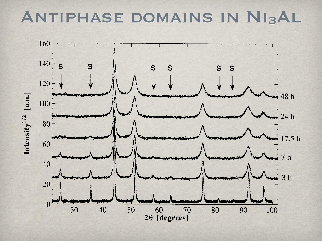
Antiphase domains in Ni3Al

!" #""$%&' () *+& ,&-)&%&)* ./ *+& "0&1*,#2 *+&,&(" ). 3#,(#*(.) ./ *+& 0#**&,) 4(*+ *+& #5(%$*+#6#)76&8 9)& 4#: *. 6..; #* *+(" 0.6& -7$,& (" <:*+();()7 *+#* *+& ()*&)"(*: #* *+& !2 " (" 0,.=0.,*(.)#6 *. *+& )$%<&, ./ 1,:"*#66(*&" .,(&)*&'#6.)7 *+& ).,%#6 06#)& *. *+& >!"#? '(,&1*(.)2 4+(1+(" 0#,#66&6 *. *+& '(,&1*(.) ('&)*(-&' <: *+&"& #)76&"8

@+& ).,%#6(5&' ()*&)"(*: #""$%&" # 3#6$& &A$#6 *. B/., # ,#)'.%6: .,(&)*&' "#%06&8C,.% C(78 D 4& 1#) ,&1.7)(5& *+#* *+& BE8D +

"#%06& "+.4" # )&#, FBBGH ., FIIGH 0,&/&,,&' .,(&)=*#*(.)8 !""$%()7 *+#* *+& 06#*&6(;& 7,#()" 0(6& $0 ()*+& "#%06& +.6'&, #6.)7 *+&(, <#"& 06#)&"2 4& 1#)1.)16$'& *+#* *+& %#() #J&" ./ *+& 7,#() #,& 0#,#66&6

C(78 K8 @,&)' ./ *+& '(L,#1*(.) "0&1*,# #* !M G! /., *+& "#%06&" %(66&' /., ()1,&#"()7 *(%&N *+& 6#<&6 O('&)*(-&" *+& "$0&,"*,$1*$,& ,&P&J&"N '.*" ,&0,&"&)* *+& &J0&,(%&)*#6 0.()*"2 6()&" *+& -**()7 /$)1*(.)"8

C(78 Q8 R(7+* ./ *+& BD "0&1*,# #* '(L&,&)* ! #)76&"2 /., *+& 0.4'&, <#66=%(66&' /., BE8D +2 1.66&1*&' *.%&#"$,& *+& *&J*$,& ./ *+& "#%06&N *+& -**()7 (" ,&0,&"&)*&' <: 6()&"8

ST@@RU9@@V #)' WV!S!XRSS!Y Z[!U!Z@RUV\!@V9X ]^ _U`BGa

Stacking/deformation faults

Warren treatment (FCC)

Peak shift:

Peak broadening:

Peak asymmetry:

!(2" ) = 90 3(#' $#")tan"% 2h02 (u + b)

(±L0 )b& !

1Deff

=1D+1.5(!' +!") + "'[ ]

ah0 (u + b)L0

b# !

y2 ! y1 =2A(4.5""+#' )c2x2 3$ (u + b)

(±) L0L0b

%

c2 = 1+&

4$Deff sin '0 + x2( ) ! sin'0[ ]( ) *

+ , -

2 !

h02 = h2 + k 2 + l 2 !

L0=h+k+lb=number broadened reflectionsu=number unbroadened reflections

α′=intrinsic faults probabilityα″=extrinsic faults probabilityβ=twin faults probability

y1

y2

x2

y1

y2

x2

Faults for other close packed structures

FCC: twin, intrinsic and extrinsic faults probabilities

BCC: no distinction intrinsic from extrinsic

HCP: twin, intrinsic and extrinsic faults probabilities

Planar dfects in beta-brass

Stacking and deformation faults modeled using the

Warren model

No faults assumed (deformation, twin etc.)

Order-disorder transition in intermetallic

Applications:High temperature structural materialOxidation resistanceBlade material for Gas turbine

Main problem:Ductility (forming and shaping)Brittle at low temperatureDisordered phase is more ductile

Materials:FeAl, Ni3Al, NiAl, TiAl...

Disordering FeAl by ball-milling

0

50

100

150

200

30 40 50 60 70 80 90 100

Inte

nsity

-1/2

[cou

nts-1

/2]

2θ [degrees]

0.5 h

1.5 h

3 h

6 h

12 h

0 h

Faults effect

0

100

200

300

400

500

70 75 80 85 90 95 100

Inte

nsity

(cou

nts)

2θ (degrees)

a)

70 75 80 85 90 95 1002θ (degrees)

b)

Anisotropic size model Faulting model (Warren)

Defect analysis on ball-milled FeAl

0.0

0.2

0.4

0.6

0.8

1.0

0.00

0.01

0.02

0.03

0.04

0 10 20 30 40 50

LRO

Deformation faulting (intrinsic)Deformation faulting (extrinsic)Twin faultingAntiphase domain

Long

Ran

ge O

rder

Deform

ation faulting probability

Milling time [h]0

50

100

150

200

250

0.000

0.001

0.002

0.003

0.004

0 10 20 30 40 50

Crystallite sizeMicrostrain

Cry

stal

lite

size

[nm

]

Microstrain

Milling time [h]

FeAl annealing (neutron-XRD meas.)

0.000

0.200

0.400

0.600

0.800

1.000

0.00

0.01

0.02

0.03

0.04

0.05

0 100 200 300 400 500 600 700 800

LRO XRD (RT measurments)LRO neutron

Deformation faultsMicrostrainAntiphase

LRO

Defects

Temperature [˚C]

Smectites structure

Clay Minerals (1984) 19, 177-193

THE D I S T R I B U T I O N OF O C T A H E D R A L C A T I O N S IN T H E 2:1 L A Y E R S O F D I O C T A H E D R A L

S M E C T I T E S S T U D I E D BY O B L I Q U E - T E X T U R E E L E C T R O N D I F F R A C T I O N

S. I . T S I P U R S K Y AND V. A. D R I T S

Geological Institute of the USSR Academy of Sciences, Pyzhevsky per. 7, Moscow, USSR

(Received 19 January 1983; revised 26 September 1983)

ABSTRACT: Olique-texture electron diffraction examination of K-saturated dioctahedral smectites after 70-100 wetting-drying cycles allows the determination of cation distribution between trans and cis octahedra of the 2:1 layers. Studies of smectites with different compositions has revealed a wide variety of occupancies of the available octahedral sites.

In dioctahedral phyllosilicates only two of the three symmetrically independent octahedral positions are occupied by cations. The 2:1 layer will have a centre of symmetry if the trans octahedra are vacant (model 1, Fig. la) and it will have none if the cations occupy trans octahedral sites as well as cis octahedral positions, forming one of the two regular systems of points (model 2, Fig. lb). Numerous structure refinements of dioctahedral layer-silicates have shown that the octahedral cations occupy only the cis octahedrat positions of the 2:1 layers if the total number of these cations per unit cell is equal to 4. The probable existence of two-layer micas with non-centrosymmetrical layers was noted by B. B. Zvyagin et al. (1979); these authors also specified the possible polytypes of micas with such layers and calculated their diffraction data for ideal models.

FIG. 1. (001) projections of octahedra and adjacent tetrahedra of 2 : 1 layer. (a) Cis octahedra are occupied (model 1). (b) Cis octahedral positions, forming one of the two regular systems of

points, are vacant; trans octahedra are occupied (model 2).

9 1984 The Mineralogical Society

Clay Minerals (1984) 19, 177-193

THE D I S T R I B U T I O N OF O C T A H E D R A L C A T I O N S IN THE 2:1 L A Y E R S O F D I O C T A H E D R A L

S M E C T I T E S S T U D I E D BY O B L I Q U E - T E X T U R E E L E C T R O N D I F F R A C T I O N

S. I . T S I P U R S K Y AND V. A. D R I T S

Geological Institute of the USSR Academy of Sciences, Pyzhevsky per. 7, Moscow, USSR

(Received 19 January 1983; revised 26 September 1983)

ABSTRACT: Olique-texture electron diffraction examination of K-saturated dioctahedral smectites after 70-100 wetting-drying cycles allows the determination of cation distribution between trans and cis octahedra of the 2:1 layers. Studies of smectites with different compositions has revealed a wide variety of occupancies of the available octahedral sites.

In dioctahedral phyllosilicates only two of the three symmetrically independent octahedral positions are occupied by cations. The 2:1 layer will have a centre of symmetry if the trans octahedra are vacant (model 1, Fig. la) and it will have none if the cations occupy trans octahedral sites as well as cis octahedral positions, forming one of the two regular systems of points (model 2, Fig. lb). Numerous structure refinements of dioctahedral layer-silicates have shown that the octahedral cations occupy only the cis octahedrat positions of the 2:1 layers if the total number of these cations per unit cell is equal to 4. The probable existence of two-layer micas with non-centrosymmetrical layers was noted by B. B. Zvyagin et al. (1979); these authors also specified the possible polytypes of micas with such layers and calculated their diffraction data for ideal models.

FIG. 1. (001) projections of octahedra and adjacent tetrahedra of 2 : 1 layer. (a) Cis octahedra are occupied (model 1). (b) Cis octahedral positions, forming one of the two regular systems of

points, are vacant; trans octahedra are occupied (model 2).

9 1984 The Mineralogical Society

Smectite layers and interlayers waterare worse than those obtained with the TOPAS refinement.This is because the latter result was accomplished with aneffective but empirical correction, which lacks physicalmeaning. WithDIFFaX+ the price to pay to retain the physicalmeaning of the calculated model of structure disorder is a lessgood fit.

The refined coordinates were used to draw the crystalstructure of the trans-vacant layer (Fig. 6a). The structure plotwas rotated by 10.5! around the b axis of the monoclinicsystem. With the rotation, it is possible to appreciate thesingularity obtained with the atomic position refinement.Some of the O atoms of the tetrahedral layer tend to be shiftedtowards the interlayer region, giving a corrugated aspect to thetetrahedral layer.

Since the occupancy of the K atoms is lower than 100%, andthe literature formulates the hypothesis of the presence ofwater in the interlayer region of illite, another refinement wasattempted, including the water molecules. In the interlayervolume, the only site for the water molecules is the same cavitythat hosts the K atoms. Other sites within the interlayervolume were explored but ruled out because of steric reasons,as the distances between the cations and the framework Oatoms would have been too short. The molecule was includedas an O atom in the same position as the K atoms and itspopulation refined. With this refinement, the agreementfactors (Rwp = 21.50%) slightly decreased. As for the K atom,the average distance between the O atom of the water mole-cule and the basal O atoms of the tetrahedral layer is 3.026 A.For the sake of completeness, an H atom was also included inthe structure model. The best position in the interlayer regionof an ideal monoclinic 1M cell was searched using the programValist (Wills & Brown, 1999), developed for locating hydrogenbonds with bond valence analysis. The calculated H-atom(Hw) coordinates were included in the refinement and keptfixed during the refinement of the other parameters. Theobtained values for the O—H distance (0.98 A) and H—O—Hangle (104.41!) of the water molecule (see again Table 5) areclose to the expected values. The distance of the H atom from

the tetrahedral O atoms is 1.92 A and the O—H" " "O angle is149.11!. These values are in accordance with the results foundfor water in other clay minerals (Sposito et al., 1999; Boek &Sprik, 2003; Hou et al., 2003; Wang et al., 2004), where thechemical environment of water in the interlayer region wasstudied using a total radial distribution function (RDF). In thecase of montmorillonites (Na and K montmorillonite), Sposito

research papers

J. Appl. Cryst. (2008). 41, 402–415 Alessandro F. Gualtieri et al. # The clay mineral illite-1M 411

Figure 6The plot of the refined structure model of illite-1M rotated by 10.5!

around the b axis of the monoclinic system in order to appreciate thesingularity obtained with the atomic position refinement. In fact, basalatoms O1 and O2 of the tetrahedral layer tend to be shifted, giving acorrugated aspect to the tetrahedral layer. (a) The structure with theinterlayer K atoms; (b) the structure with the interlayer water moleculewith O" " "H contacts.

Figure 5The graphical output of the refinement using DIFFaX+, with theobserved, the calculated and the difference curve. See text for details.

Gualtieri et al., J. Appl. Cryst., (2008) 41, 402-415

How to work with the disorderVIANI ET AL.: NATURE OF DISORDER IN MONTMORILLONITE972

tions S12-S14) poorly reproduce the intermediate 15–25 2region and correctly broaden the high angle (35–60 2) re-gion. The mixed models (simulations S15-S17) yield a satis-factory match with the full observed pattern (especiallysimulation S16) although some extra inconsistent peaks are stillobserved at 12.5, 24, and 42 2.

Rotations between adjacent layers which preserve the su-perposition of basal O atoms of adjacent layers have been con-sidered in the simulation series in Figure 8 (see the probabilitymatrices in Table 4). Drits et al. (1984) have shown that mica-like stacking may lead to azimuthal defects corresponding to120 and 60 rotations of successive layers and that the usualcoordination of the compensating cation K is kept in the caseof 120 rotations while it becomes prismatic in the case of60 rotations. The simulations with 60 rotations only are S18-S19, and the simulations with only 120 rotations only are S20-S21. This simulation is in agreement with that reported in Figure14(b) in Drits et al. (1984) for the same system showing theappearance of a sharp broad band at 22.3 2. The simulations

with randomly mixed 60 and 120 rotations are S22-S24. It isclear that a model of disorder based only on rotations is unsat-isfactory because either the low-intermediate or the high angleregions are poorly modeled. In addition, the peaks at 3.8 and2.5 Å are always largely overestimated.

DISCUSSION AND FINAL MODEL OF DISORDER

The model of disorder of this Ca-montmorillonite samplemay not be directly applied to all montmorillonite samples be-cause, as reported by Weizong et al. (2000), the structure of theclay mineral quasi-crystals depends strongly on the exchange-able cation and H2O content. Notwithstanding, the workingstrategy presented here can be successfully utilized for mont-morillonite and complex 2:1 clay samples of different natureand this approach can be combined with the method proposedby Reynolds (1993), McCarty and Reynolds (1995), and Dritsand McCarty (1996) for a quantitative determination of thecontent of single units in randomly interstratified mixed-layerstructures such as illite-smectite (I/S) to reveal diversity of il-lite and I/S samples with different conditions of formation andtransformation. In addition, it can be employed in the study ofmixed-layer phases with integrated TEM and XRD (Guthrieand Reynolds 1998) in an attempt to better account for dis-crepancies in structure descriptions based only on one tech-nique.

The preliminary structure simulations that consider the varia-tion of all factors which may contribute to the broadening ofthe diffraction peaks of montmorillonite indicate that a com-plex model should be used in order to reproduce the observedpowder pattern. To this end, we performed simulations with acombination of shifts and rotations, shifts and disordered Alvacancies, and rotations and disordered Al vacancies. In addi-tion, disordering of the Ca atoms and water molecules was alsotaken into account. Table 5 reports the probability matrices ofsome selected simulations. In addition to the instrumental con-tribution, the microstructural broadening was also consideredto perfectly reproduce the peak broadening in the observedpattern. Consequently, a finite number of six to seven 15 Åthick layers corresponding to about 10 nm thickness (size ofthe coherent diffracting domains) was stacked along c in agree-ment with the TEM images and surface area.

Unfortunately, as previously mentioned, our simulationscannot be directly compared with those reported in Drits et al.(1984) because they selected a dehydrated K-saturated mont-morillonite system to study the effects of combined disorderedmodels.

Figure 9 shows some selected simulated powder patternswith combinations of shifts and rotations (see the relative prob-ability matrix in Table 5). The Ca atoms are located in the hex-agonal cavities. Pattern S25 clearly shows large differences inpeak intensities in the 16–25 2 region and the presence ofthe (002) reflection which is not observed in the experimentalpattern. The same applies to patterns S26, S27, and S28 al-though in these cases a better fit of the 16–25 2 region wasaccomplished.

The model which gives the best fit of the observed data (Rp

= 0.267) was obtained introducing random shifts along b/3and –a/3 (see the probability matrix in Table 5) with a total

FIGURE 7. Set of DIFFaX structure simulations of models withtranslational disorder along b/3, a/3, and combined b/3 and a/3.

FIGURE 8. Set of DIFFaX structure simulations of models withrotations between adjacent layers of 60, 120, and combined60 and 120.

Viani et al., (2002), Am. Miner., 87, 966-975

DiffaX+ simulation

are worse than those obtained with the TOPAS refinement.This is because the latter result was accomplished with aneffective but empirical correction, which lacks physicalmeaning. WithDIFFaX+ the price to pay to retain the physicalmeaning of the calculated model of structure disorder is a lessgood fit.

The refined coordinates were used to draw the crystalstructure of the trans-vacant layer (Fig. 6a). The structure plotwas rotated by 10.5! around the b axis of the monoclinicsystem. With the rotation, it is possible to appreciate thesingularity obtained with the atomic position refinement.Some of the O atoms of the tetrahedral layer tend to be shiftedtowards the interlayer region, giving a corrugated aspect to thetetrahedral layer.

Since the occupancy of the K atoms is lower than 100%, andthe literature formulates the hypothesis of the presence ofwater in the interlayer region of illite, another refinement wasattempted, including the water molecules. In the interlayervolume, the only site for the water molecules is the same cavitythat hosts the K atoms. Other sites within the interlayervolume were explored but ruled out because of steric reasons,as the distances between the cations and the framework Oatoms would have been too short. The molecule was includedas an O atom in the same position as the K atoms and itspopulation refined. With this refinement, the agreementfactors (Rwp = 21.50%) slightly decreased. As for the K atom,the average distance between the O atom of the water mole-cule and the basal O atoms of the tetrahedral layer is 3.026 A.For the sake of completeness, an H atom was also included inthe structure model. The best position in the interlayer regionof an ideal monoclinic 1M cell was searched using the programValist (Wills & Brown, 1999), developed for locating hydrogenbonds with bond valence analysis. The calculated H-atom(Hw) coordinates were included in the refinement and keptfixed during the refinement of the other parameters. Theobtained values for the O—H distance (0.98 A) and H—O—Hangle (104.41!) of the water molecule (see again Table 5) areclose to the expected values. The distance of the H atom from

the tetrahedral O atoms is 1.92 A and the O—H" " "O angle is149.11!. These values are in accordance with the results foundfor water in other clay minerals (Sposito et al., 1999; Boek &Sprik, 2003; Hou et al., 2003; Wang et al., 2004), where thechemical environment of water in the interlayer region wasstudied using a total radial distribution function (RDF). In thecase of montmorillonites (Na and K montmorillonite), Sposito

research papers

J. Appl. Cryst. (2008). 41, 402–415 Alessandro F. Gualtieri et al. # The clay mineral illite-1M 411

Figure 6The plot of the refined structure model of illite-1M rotated by 10.5!

around the b axis of the monoclinic system in order to appreciate thesingularity obtained with the atomic position refinement. In fact, basalatoms O1 and O2 of the tetrahedral layer tend to be shifted, giving acorrugated aspect to the tetrahedral layer. (a) The structure with theinterlayer K atoms; (b) the structure with the interlayer water moleculewith O" " "H contacts.

Figure 5The graphical output of the refinement using DIFFaX+, with theobserved, the calculated and the difference curve. See text for details.Gualtieri et al., J. Appl. Cryst., (2008) 41, 402-415

Using pair distribution function (PDF)

The results of the structure refinements using GSAS andTOPAS confirm the limits of the Rietveld method withstructures affected by planar disorder such as clay minerals.The problem has already been discussed in the literature (e.g.Viani et al., 2002) and resides in the inability to reproducecorrectly the anisotropic peak broadening due to the planardisorder and to give a physical meaning to it. It is obvious that

the empirical corrections for anisotropic broadening not onlylack physical consistency but also misinterpret the scatteringfrom the disordered crystals. The structural information issomehow hidden in the peak profiles. The Rietveld programsare not specifically developed to deal with highly defectivestructures, simply because, to date, there have been no specificalgorithms implemented to model planar disorder. There areactually specific algorithms for the empirical anisotropicbroadening of the peak profiles (such as that with the sphericalharmonics used here) but they lack physical meaning. In theRietveld method, the calculated value of the ith intensity pointof the peak profile is proportional to jFhklj2’(2!), where F isthe structure factor of the hkl(s) reflection contributing to thatintensity; ’(2!) is the reflection profile function, whichincludes isotropic (instrumental function) and empiricalanisotropic (microstructure) contributions. For illite and adisordered clay phase in general, the ith intensity pointof the peak profile should be instead proportional tojFhklj2jFh0k0l 0j2’(2!)’(2!hkl), where Fhkl is the structure factorof the hkl(s) reflection not affected by (planar) disorder; Fh0k0l 0

is the structure factor of the h0k0l0(s) family of reflectionsaffected by (planar) disorder. In the case of a constant struc-ture factor per layer, the interference function is related to theprobability correlation function, which describes the stackingordering of the layers. A noncrystallographic aperiodicalmathematical model and formalism is needed; ’(2!) is thereflection profile function that includes an isotropic instru-mental contribution; ’(2!hkl) is the reflection profile functionthat includes an anisotropic contribution arising due to crystalsize/shape.

Except for the mismatch of the number of cells stackedalong c, calculated with NEWMOD and WILDFIRE, thestructural information obtained from the simulations wasconfirmed by the results obtained with DIFFaX+.

Because PDFFIT does not handle stacking-fault disordercorrectly, only the first shell of the tetrahedral and octahedralatoms in the PDF curve, unaffected by structure disorder, willbe correctly fitted. Keeping this in mind, it is very promisingthat the interatomic distances for the first shell around thetetrahedral (T) atoms, octahedral (O) atoms and compen-

research papers

J. Appl. Cryst. (2008). 41, 402–415 Alessandro F. Gualtieri et al. ! The clay mineral illite-1M 413

Figure 8The G(r) curve up to about 3 A, generated by the atomic species in thebasic unit not affected by planar disorder.

Figure 7The results of the PDFFIT refinement, with the observed data, thecalculated reduced RDF curves, and the difference curve, calculated (a)with the starting model from TOPAS, (b) with the starting model fromDIFFaX+, and (c) with all the other parameters (lattice parameters,occupancy of the K atom and the water molecule, ADPs) refined.

The results of the structure refinements using GSAS andTOPAS confirm the limits of the Rietveld method withstructures affected by planar disorder such as clay minerals.The problem has already been discussed in the literature (e.g.Viani et al., 2002) and resides in the inability to reproducecorrectly the anisotropic peak broadening due to the planardisorder and to give a physical meaning to it. It is obvious that

the empirical corrections for anisotropic broadening not onlylack physical consistency but also misinterpret the scatteringfrom the disordered crystals. The structural information issomehow hidden in the peak profiles. The Rietveld programsare not specifically developed to deal with highly defectivestructures, simply because, to date, there have been no specificalgorithms implemented to model planar disorder. There areactually specific algorithms for the empirical anisotropicbroadening of the peak profiles (such as that with the sphericalharmonics used here) but they lack physical meaning. In theRietveld method, the calculated value of the ith intensity pointof the peak profile is proportional to jFhklj2’(2!), where F isthe structure factor of the hkl(s) reflection contributing to thatintensity; ’(2!) is the reflection profile function, whichincludes isotropic (instrumental function) and empiricalanisotropic (microstructure) contributions. For illite and adisordered clay phase in general, the ith intensity pointof the peak profile should be instead proportional tojFhklj2jFh0k0l 0j2’(2!)’(2!hkl), where Fhkl is the structure factorof the hkl(s) reflection not affected by (planar) disorder; Fh0k0l 0

is the structure factor of the h0k0l0(s) family of reflectionsaffected by (planar) disorder. In the case of a constant struc-ture factor per layer, the interference function is related to theprobability correlation function, which describes the stackingordering of the layers. A noncrystallographic aperiodicalmathematical model and formalism is needed; ’(2!) is thereflection profile function that includes an isotropic instru-mental contribution; ’(2!hkl) is the reflection profile functionthat includes an anisotropic contribution arising due to crystalsize/shape.

Except for the mismatch of the number of cells stackedalong c, calculated with NEWMOD and WILDFIRE, thestructural information obtained from the simulations wasconfirmed by the results obtained with DIFFaX+.

Because PDFFIT does not handle stacking-fault disordercorrectly, only the first shell of the tetrahedral and octahedralatoms in the PDF curve, unaffected by structure disorder, willbe correctly fitted. Keeping this in mind, it is very promisingthat the interatomic distances for the first shell around thetetrahedral (T) atoms, octahedral (O) atoms and compen-

research papers

J. Appl. Cryst. (2008). 41, 402–415 Alessandro F. Gualtieri et al. ! The clay mineral illite-1M 413

Figure 8The G(r) curve up to about 3 A, generated by the atomic species in thebasic unit not affected by planar disorder.

Figure 7The results of the PDFFIT refinement, with the observed data, thecalculated reduced RDF curves, and the difference curve, calculated (a)with the starting model from TOPAS, (b) with the starting model fromDIFFaX+, and (c) with all the other parameters (lattice parameters,occupancy of the K atom and the water molecule, ADPs) refined.

Gualtieri et al., J. Appl. Cryst., (2008) 41, 402-415

The material

• STx-1 Ca-montmorillonite from Texas (american Clay Society)

• Samples prepared by cold pressing (uniaxial)

• Sample 1: 10 MPa / 7 days (porosity: 36.5 %)

• Sample 2: 15 MPa / 10 days (porosity: 17.4 %)

Slab of 3 mm cut from the compressed cylinder

BESSRC 11-ID-C (with Mar345 image plate detector)

Transmission geometry

λ = 0.107877 Å

Compression axis perpendicular to beam

XRD measurement at APS (Argonne)

Rietveld texture analysis

• Maud program: images sampled in 72 patterns

• Crystal structure refinement: Rietveld with fragments

• Microstructure:

• Popa anisotropic model for crystallite sizes and microstrains

• Single Layer model for turbostratic disorder

• Texture: standard functions (EWIMV in the first step)

• Phases: Montmorillonite, Opal-CT, Quartz

Ca-montmorillonite: crystal structure refinement

Turbostratic disorder: reciprocal lattice

Ufer et al., (2004), Z. Kristallogr. 219: 519-527

Single layer model

Ufer et al., (2004)Z. Kristallogr. 219: 519-527

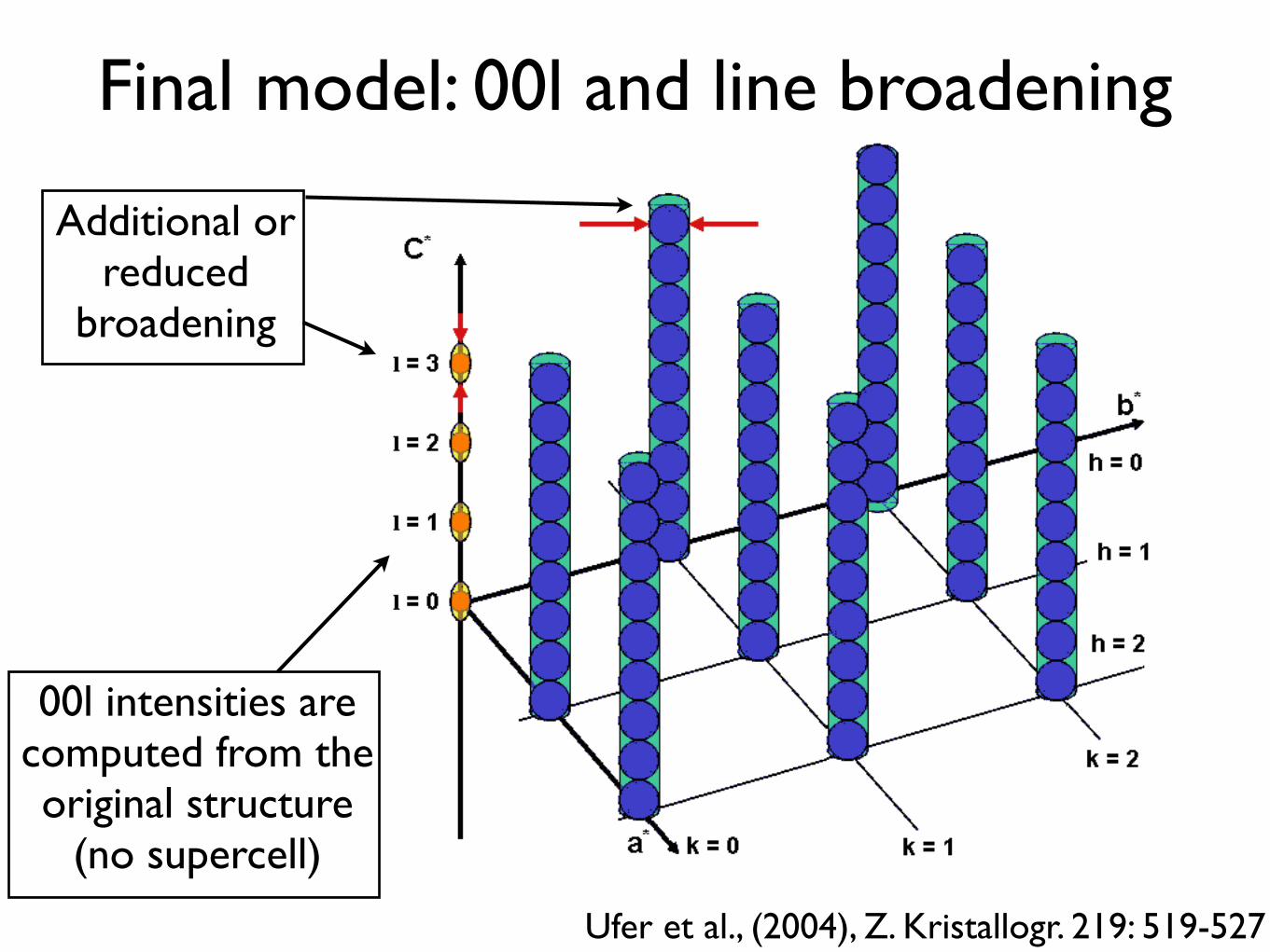
Final model: 00l and line broadening

Ufer et al., (2004), Z. Kristallogr. 219: 519-527

00l intensities are computed from the original structure

(no supercell)

Additional or reduced

broadening

Montmorillonite and single layer model

Ufer et al., (2004), Z. Kristallogr. 219: 519-527

Single layer model - ideal structure

Final crystal structure refinement

3D plot: see the texture

Sample 1

Sample 2

Comparison samples 1 and 2

1)

2)

Texture without and with SL model

No single layer model

Using single layer model

Crystallite sizes & microstrainshkl direction Crystallite size (Å) Microstrain (x10-3)

001 196 17.5

010 427 0.053

100 622 0.11

110 679 0.32

hkl direction Crystallite size (Å) Microstrain (x10-3)

001 293 22.3

010 434 0.023

100 686 0.01

110 655 1.75

Sample 1

Sample 2

The Opal-CT

calculated calculated

observed observed

15 20 25 30 35 40 15 20 25 30 35 4028 eCuKa) 28 (OCuKa)

---

870 GUTHRIE ET AL.: OPAL-CT DIFFRACTION PATTERN

acalculation parameters

N1 ~N2 = 17.3 nmN3 = 20.0 nm0= 6.1 nmPtd = 0.45 (Per = 0.55)

0c =0.55

bcalculation parametersN 1

::::; N2 = 17.3 nmN3 =20.0 nm0= 6.1 nmPtd= 0.500c = 0.55

Fig. I. Comparison of calculated and observed patterns fortwo opals. (a) Calculated for 45% tridymite and random stacking(Dc = Per); observed pattern from 46E5880. (b) Calculated for50% tridymite and 10% ordering (De> Ptd); observed patternfrom 28501. Note shoulder on high-angle side of20-25° 28 bandin b. Ordering state of the cristobalite-tridymite interstratifica-tion can be evaluated by the relationship among Dc, Ptd, and Perfor the following two cases: for Ptd ~ 0.5, Dc = Ptd for random

interstratification, Dc > Ptd for ordered interstratification (e.g.,De= 1 produces R1 ordering), and Dc < Ptd for segregation (e.g.,Dc = 0 produces complete segregation of cristobalite and tridy-mite layers); for Ptd < 0.5, Dc = Perfor random interstratification,Dc > Per for ordered interstratification, and Dc < Per for segre-gation. The two cases result from the way in which the junctionprobabilities are defined. More detailed discussions of probabil-ities and interstratification are found in Reynolds (1980, 1993).

ing problems. First, modeling can provide support for thehypothesis that opal is an interstratification of cristobaliteand tridymite and can provide constraints on the rangeof structural states found in opal. Second, by modelingthe diffraction patterns for suites of different opal samplesrepresenting likely diagenetic sequences, one can identifyappropriate methods for monitoring the maturation ofopal. The current approach to monitoring opal matura-tion uses the position of the ""'21.70 peak (typically re-ported as dID.)' which migrates from 0.412 to 0.404 nmduring diagenesis (Murata and Nakata, 1974). Modelingmay reveal the reason for this peak shift. Finally, resultsfrom modeling the diffraction pattern for a particular opalcan be used in conjunction with Rietveld methods to de-termine quantitative mineral abundances.We have modeled the opal diffraction pattern as an

interstratification of cristobalite and tridymite. Our mod-eling approach allows the variation of particle size, pro-portions of the two different layers, and ordering state(from segregated layers to disordered interstratificationsto R I-ordered interstratifications, where complete R 1 or-dering refers to a rigorous alternation of the two layertypes). Graetsch et al. (1994) attempted to model the dif-fraction pattern of opal-CT using a simulation programby Treacy et al. (1991). They calculated images for sev-eral proportions of tridymite and cristobalite layers (whichthey referred to as representing "various degrees of stack-ing disorder"); however, they apparently did not considerR 1 ordering as a parameter in their calculations. In otherwords, their "ordering" refers to the relative probabilitiesof the two types of layers and not to an ordered inter-stratification. In this paper, we present our modeling re-sults in detail and show that they can be used to addressmany of the problems outlined above. We also compare

our modeling results with the XRD patterns of severalnatural opal samples to demonstrate the success of themodel and to illustrate the likely ranges in structural states.

METHODSDiffraction patterns were calculated using a modified

version of the program Wildfire (R. C. Reynolds, Hano-ver, New Hampshire), which has been applied success-fully to the modeling of three-dimensional XRD patternsof interstratified clays. The details of the computationalmethod used by Wildfire are discussed by Reynolds (1980,1993). In short, Wildfire simulates the XRD patterns ofinterstratified layer structures by calculating the Fouriertransform of individual layers and by assembling the in-tergrowth structure in reciprocal space. The contributionfrom each layer is summed statistically to form the recip-rocallattice of a "virtual crystal" that is representative ofa distribution of crystals with various proportions of eachlayer type and various ordering states and crystallite sizes.In our opal calculations, the variables included the fol-lowing: probability of tridymite (Ptd), probability of cris-tobalite (Per= 1 - Ptd),maximum crystallite size alongthe stacking direction c (N3),mean value of the crystallitesize along c (0), crystallite size along a (N.) and b (N2),and ordering coefficient (OJ. The significance of the or-dering coefficient is described in the Figure 1 caption.Calculations were performed for A= 0.15418 nm (i.e., tosimulate CuKa radiation).The structure of the layer used in our calculations is an

idealized sheet, as found in the high-temperature struc-tures of cristobalite and tridymite. The dimensions of thesheet were adjusted so that the positions of the calculatedpeaks matched those observed. Tridymite stacking was

Tridymite+cristobalite intermixed (using Wildfire)

It is disordered too!

Guthrie et al., (1995) Am. Miner. 80, 869-872.

How to compute Opal-CTIdeal cristobalite (HT)

Ideal tridymite (HT)

In analogy with faults in FCC/HCP:

abcababcba....

Hexagonal tridymite disordered by SL

Quantitative phase analysis

Sample Opal-CT Quartz

1 8% 0.2%

2 7% 0.3%

Other results

• No Al in cis-sites

• Water/Ca occupation around 40%

Carbon-carbon composites

ZnO: 4%Carbon matrix: 76%Carbon fibers: 20%

Warren-Averbach

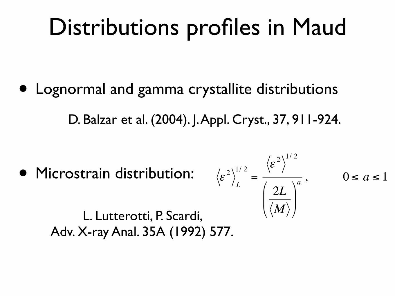
Distributions profiles in Maud

• Lognormal and gamma crystallite distributions

• Microstrain distribution:

D. Balzar et al. (2004). J. Appl. Cryst., 37, 911-924.

L. Lutterotti, P. Scardi, Adv. X-ray Anal. 35A (1992) 577.

€

ε 2L

1/ 2=

ε 2 1/ 2

2LM

#

$ %

&

' (

a , 0 ≤ a ≤ 1

research papers

340 Popa and Balzar ✏ Size-broadened profile J. Appl. Cryst. (2002). 35, 338±346

DA à �1= � 0

Ö0Ü à 4�3=3�2: Ö8Ü

4. Application to size distributions

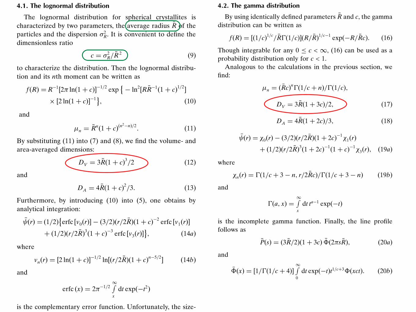
4.1. The lognormal distribution

The lognormal distribution for spherical crystallites ischaracterized by two parameters, the average radius �R of theparticles and the dispersion �2R. It is convenient to deÆne thedimensionless ratio

c à �2R= �R2

Ö9Ü

to characterize the distribution. Then the lognormal distribu-tion and its nth moment can be written as

f ÖRÜ à R�1â2⇡ lnÖ1á cÜä�1=2 exp

�� ln2âR �R�1

Ö1á cÜ1=2ä

⇥ â2 lnÖ1á cÜä�1 ; Ö10Ü

and

�n à�RnÖ1á cÜÖn

2�nÜ=2: Ö11Ü

By substituting (11) into (7) and (8), we Ænd the volume- andarea-averaged dimensions:

DV à 3 �RÖ1á cÜ3=2 Ö12Ü

and

DA à 4 �RÖ1á cÜ2=3: Ö13Ü

Furthermore, by introducing (10) into (5), one obtains byanalytical integration:

� ÖrÜ à Ö1=2Ü�erfc âv0ÖrÜä � Ö3=2ÜÖr=2 �RÜÖ1á cÜ

�2 erfc âv1ÖrÜä

á Ö1=2ÜÖr=2 �RÜ3Ö1á cÜ�3 erfc âv3ÖrÜä

; Ö14aÜ

where

vnÖrÜ à â2 lnÖ1á cÜä�1=2 lnâÖr=2 �RÜÖ1á cÜn�5=2

ä Ö14bÜ

and

erfc ÖxÜ à 2⇡�1=2R1

x

dt expÖ�t2Ü

is the complementary error function. Unfortunately, the size-broadened proÆle can not be calculated analytically by theFourier transform of (14), or by direct integration of (6). Forthe numerical computation, the integral (6), after the intro-duction of (10), must be reduced to a standard quadratureformula. By using simple transformations of the integrationvariable, one obtains

�PÖsÜ à Ö3 �R=2ÜÖ1á cÜ3 ��Ö2⇡s �RÜ; Ö15aÜ

and

��ÖxÜ à ⇡�1=2R1

�1

dt expÖ�t2Ü��xÖ1á cÜ7=2 expftâ2 lnÖ1á cÜä1=2g

�:

Ö15bÜ

This integral can be computed by a standard Gauss±Hermitequadrature.

4.2. The gamma distribution

By using identically deÆned parameters �R and c, the gammadistribution can be written as

f ÖRÜ à âÖ1=cÜ1=c= �R�Ö1=cÜäÖR= �RÜ1=c�1 expÖ�R= �RcÜ: Ö16Ü

Though integrable for any 0 c < 1, (16) can be used as aprobability distribution only for c < 1.

Analogous to the calculations in the previous section, weÆnd:

�n à Ö

�RcÜn�Ö1=cá nÜ=�Ö1=cÜ;

DV à 3 �RÖ1á 3cÜ=2; Ö17Ü

DA à 4 �RÖ1á 2cÜ=3; Ö18Ü

� ÖrÜ à �0ÖrÜ � Ö3=2ÜÖr=2 �RÜÖ1á 2cÜ�1�1ÖrÜ

á Ö1=2ÜÖr=2 �RÜ3Ö1á 2cÜ�1Ö1á cÜ�1�3ÖrÜ; Ö19aÜ

where

�nÖrÜ à �Ö1=cá 3� n; r=2 �RcÜ=�Ö1=cá 3� nÜ Ö19bÜ

and

�Öa; xÜ àR1

x

dt ta�1 expÖ�tÜ

is the incomplete gamma function. Finally, the line proÆlefollows as

�PÖsÜ à Ö3 �R=2ÜÖ1á 3cÜ ��Ö2⇡s �RÜ; Ö20aÜ

and

��ÖxÜ à â1=�Ö1=cá 4ÜäR1

0

dt expÖ�tÜt1=cá3�ÖxctÜ: Ö20bÜ

This integral can be computed by a standard Gauss±Laguerrequadrature, except for very small values of c, when thecomputation errors become signiÆcant. However, for small c,the gamma and lognormal distributions become indis-tinguishable [compare for example (17) with (12)], and onecan use (15b) instead of (20b) to calculate ��.

5. Determination of the distribution parameters

One can useDV andDA, obtained from the Fourier analysis ofline proÆles, to calculate values of �R and c by using (12) and(13) for the lognormal distribution (Krill & Birringer, 1998) or(17) and (18) for the gamma distribution. However, except formaterials with the highest crystallographic symmetry, lineproÆles commonly overlap, which makes it necessary toreconstruct overlapped proÆle tails, usually by proÆle Ætting ofsimple analytical functions (Voigt or its approximations).

Another possibility to determine the size distributionparameters is to multiply (14) [or (19)] by the distortion(strain) Fourier coefÆcients and then Æt the result to theFourier transform of experimental diffraction proÆles,corrected with the Fourier transform of the instrumentalcontribution (Unga¬r et al., 2001). However, in cases of

research papers

340 Popa and Balzar ✏ Size-broadened profile J. Appl. Cryst. (2002). 35, 338±346

DA à �1= � 0

Ö0Ü à 4�3=3�2: Ö8Ü

4. Application to size distributions

4.1. The lognormal distribution

The lognormal distribution for spherical crystallites ischaracterized by two parameters, the average radius �R of theparticles and the dispersion �2R. It is convenient to deÆne thedimensionless ratio

c à �2R= �R2

Ö9Ü

to characterize the distribution. Then the lognormal distribu-tion and its nth moment can be written as

f ÖRÜ à R�1â2⇡ lnÖ1á cÜä�1=2 exp

�� ln2âR �R�1

Ö1á cÜ1=2ä

⇥ â2 lnÖ1á cÜä�1 ; Ö10Ü

and

�n à�RnÖ1á cÜÖn

2�nÜ=2: Ö11Ü

By substituting (11) into (7) and (8), we Ænd the volume- andarea-averaged dimensions:

DV à 3 �RÖ1á cÜ3=2 Ö12Ü

and

DA à 4 �RÖ1á cÜ2=3: Ö13Ü

Furthermore, by introducing (10) into (5), one obtains byanalytical integration:

� ÖrÜ à Ö1=2Ü�erfc âv0ÖrÜä � Ö3=2ÜÖr=2 �RÜÖ1á cÜ

�2 erfc âv1ÖrÜä

á Ö1=2ÜÖr=2 �RÜ3Ö1á cÜ�3 erfc âv3ÖrÜä

; Ö14aÜ

where

vnÖrÜ à â2 lnÖ1á cÜä�1=2 lnâÖr=2 �RÜÖ1á cÜn�5=2

ä Ö14bÜ

and

erfc ÖxÜ à 2⇡�1=2R1

x

dt expÖ�t2Ü

is the complementary error function. Unfortunately, the size-broadened proÆle can not be calculated analytically by theFourier transform of (14), or by direct integration of (6). Forthe numerical computation, the integral (6), after the intro-duction of (10), must be reduced to a standard quadratureformula. By using simple transformations of the integrationvariable, one obtains

�PÖsÜ à Ö3 �R=2ÜÖ1á cÜ3 ��Ö2⇡s �RÜ; Ö15aÜ

and

��ÖxÜ à ⇡�1=2R1

�1

dt expÖ�t2Ü��xÖ1á cÜ7=2 expftâ2 lnÖ1á cÜä1=2g

�:

Ö15bÜ

This integral can be computed by a standard Gauss±Hermitequadrature.

4.2. The gamma distribution

By using identically deÆned parameters �R and c, the gammadistribution can be written as

f ÖRÜ à âÖ1=cÜ1=c= �R�Ö1=cÜäÖR= �RÜ1=c�1 expÖ�R= �RcÜ: Ö16Ü

Though integrable for any 0 c < 1, (16) can be used as aprobability distribution only for c < 1.

Analogous to the calculations in the previous section, weÆnd:

�n à Ö

�RcÜn�Ö1=cá nÜ=�Ö1=cÜ;

DV à 3 �RÖ1á 3cÜ=2; Ö17Ü

DA à 4 �RÖ1á 2cÜ=3; Ö18Ü

� ÖrÜ à �0ÖrÜ � Ö3=2ÜÖr=2 �RÜÖ1á 2cÜ�1�1ÖrÜ

á Ö1=2ÜÖr=2 �RÜ3Ö1á 2cÜ�1Ö1á cÜ�1�3ÖrÜ; Ö19aÜ

where

�nÖrÜ à �Ö1=cá 3� n; r=2 �RcÜ=�Ö1=cá 3� nÜ Ö19bÜ

and

�Öa; xÜ àR1

x

dt ta�1 expÖ�tÜ

is the incomplete gamma function. Finally, the line proÆlefollows as

�PÖsÜ à Ö3 �R=2ÜÖ1á 3cÜ ��Ö2⇡s �RÜ; Ö20aÜ

and

��ÖxÜ à â1=�Ö1=cá 4ÜäR1

0

dt expÖ�tÜt1=cá3�ÖxctÜ: Ö20bÜ

This integral can be computed by a standard Gauss±Laguerrequadrature, except for very small values of c, when thecomputation errors become signiÆcant. However, for small c,the gamma and lognormal distributions become indis-tinguishable [compare for example (17) with (12)], and onecan use (15b) instead of (20b) to calculate ��.

5. Determination of the distribution parameters

One can useDV andDA, obtained from the Fourier analysis ofline proÆles, to calculate values of �R and c by using (12) and(13) for the lognormal distribution (Krill & Birringer, 1998) or(17) and (18) for the gamma distribution. However, except formaterials with the highest crystallographic symmetry, lineproÆles commonly overlap, which makes it necessary toreconstruct overlapped proÆle tails, usually by proÆle Ætting ofsimple analytical functions (Voigt or its approximations).

Another possibility to determine the size distributionparameters is to multiply (14) [or (19)] by the distortion(strain) Fourier coefÆcients and then Æt the result to theFourier transform of experimental diffraction proÆles,corrected with the Fourier transform of the instrumentalcontribution (Unga¬r et al., 2001). However, in cases of

Dislocations distribution (spatially)

┻┻

┻┻

┻┻

┻

┻┻┻

┻

┻┻ ┻

┻┻

┻┻

┻┻

┻┻ ┻

┻ ┻┻

┻┻

┻┻

┻┻

┻

┻┻ ┻

┻┻

┻ ┻┻┻┻┻

a=1a=0

Column of cell (the crystallite)

Instrumental profile

Fourier Transform