place-based correlates of motor vehicle theft and recovery
TRANSCRIPT

City University of New York (CUNY) City University of New York (CUNY)
CUNY Academic Works CUNY Academic Works
Publications and Research John Jay College of Criminal Justice
2016
Place-based correlates of Motor Vehicle Theft and Recovery: Place-based correlates of Motor Vehicle Theft and Recovery:
Measuring spatial influence across neighbourhood context Measuring spatial influence across neighbourhood context
Eric L. Piza CUNY John Jay College
Shun Feng CUNY John Jay College
Leslie Kennedy Rutgers University - Newark
Joel Caplan Rutgers University - Newark
How does access to this work benefit you? Let us know!
More information about this work at: https://academicworks.cuny.edu/jj_pubs/224
Discover additional works at: https://academicworks.cuny.edu
This work is made publicly available by the City University of New York (CUNY). Contact: [email protected]

Article
Urban Studies1–24� Urban Studies Journal Limited 2016Reprints and permissions:sagepub.co.uk/journalsPermissions.navDOI: 10.1177/0042098016664299usj.sagepub.com
Place-based correlates of MotorVehicle Theft and Recovery:Measuring spatial influence acrossneighbourhood context
Eric PizaJohn Jay College of Criminal Justice, USA
Shun FengJohn Jay College of Criminal Justice, USA
Leslie KennedyRutgers University, USA
Joel CaplanRutgers University, USA
AbstractSocial scientists have long shown great interest in the spatial correlates of crime patterns. A sub-set of the literature has focused on how micro-level spatial factors influence the formation ofcrime hot spots. At the same time, tangential research has highlighted how neighbourhood disad-vantage influences crime occurrence. The current study focuses on the intersection of these per-spectives through a spatial analysis of Motor Vehicle Theft (MVT) and Motor Vehicle Recovery(MVR) in Colorado Springs, CO. We begin by conducting a Risk Terrain Modelling analysis toidentify spatial risk factors significantly related to MVT and MVR occurrence. We then testwhether the spatial influences of the criminogenic risk factors differ across traditional measuresof neighbourhood disadvantage. Findings suggest that while a citywide effect is evident for multi-ple risk factors, their spatial influence on crime significantly varies across neighbourhoodcontexts.
Keywordsenvironmental criminology, Motor Vehicle Recovery, Motor Vehicle Theft, Risk Terrain Modelling,social disorganisation
Received November 2015; accepted July 2016Corresponding author:
Eric Piza, John Jay College of Criminal Justice, 524 W 59th
St, Haaran Hall, Room 636.15, New York City, NY 10019,
USA.
Email: [email protected]
at JOHN JAY COLLEGE on August 24, 2016usj.sagepub.comDownloaded from

Introduction
Social scientists have long exhibited greatinterest in the geography of crime, with theexploration of crime concentration datingback hundreds of years (Weisburd et al.,2009). With the emergence of GeographicInformation Systems (GIS), the spatial analy-sis of crime has greatly accelerated. Inexplaining crime concentrations, contempo-rary research has empirically tested the influ-ence of potentially criminogenicenvironmental features on a number of crimetypes, including assault (Grubesic et al., 2012;Kennedy et al., 2015), robbery (Bernasco andBlock, 2011; Drawve, 2016), shootings(Caplan et al., 2011; Kennedy et al., 2011),and burglary (Caplan et al., 2015; Groff andLa Vigne, 2001; Moreto et al., 2014).Tangential to the crime-and-place literature,considerable research has measured the effectof neighbourhood-level factors on crime, par-ticularly violence (Kubrin and Herting, 2003;Morenoff et al., 2001; Sampson and Groves,1989; Sutherland et al., 2013). Explanatoryvariables are typically derived from data col-lected by census bureaus, which measure lev-els of neighbourhood disadvantage.
To date, Motor Vehicle Crime has beenlargely absent from the geospatial literature.The current study seeks to help fill this voidthrough an analysis of Motor Vehicle Theft(MVT) and Motor Vehicle Recovery (MVR)in Colorado Springs, CO. We begin byempirically testing the effect of various spa-tial features on the occurrence of MVT andMVR. We then test whether the influence ofthe significant risk factors differs across tra-ditional measures of neighbourhood disad-vantage. Seven spatial risk factors weresignificantly associated with MVT while tenwere associated with MVR. Subsequentmodels found that the spatial influence ofeach risk factor differed according to levelsof neighbourhood disadvantage, as mea-sured across six variables. The findings
suggest that future research should continueto measure the interaction effects of micro-level environmental risk factors and neigh-bourhood characteristics on crime patterns.
Review of relevant literature
Motor vehicle theft and recovery
MVT is one of the most commonly occur-ring crimes in the USA, with 689,527reported incidents nationwide in 2014 (FBI,2015). The literature recognises two generaltypes of MVT: (1) those committed for non-monetary purposes, such as joyriding andtransportation, and (2) those committed forprofit-driven purposes, such as resale, exportor dismantling for spare parts (Clarke andHarris, 1992; Roberts and Block, 2012). Akey difference between these typologies con-cerns the procedural nature of the crime. Inthefts for profit, offenders benefit directlyfrom the materialistic value of the vehicle,specifically through export or resale of thevehicle, or selling parts on the black market.Such incidents are more likely to be perma-nent thefts, with the stolen vehicle not beingrecovered. On the contrary, in thefts involv-ing non-monetary motivations (e.g. trans-portation and/or joyriding) benefits arelargely unrelated to the materialistic value ofthe vehicle. Stolen vehicles are more likely tobe recovered in such instances because theseoffenders are more likely to abandon thevehicle than offenders motivated by profit.
Considered from a script analysis per-spective (Cornish, 1994), the site of the vehi-cle recovery represents the final step of theMVT. The offender, after receiving thedesired benefits, abandons the vehicle. Forresearchers, stolen vehicle recovery presentsadditional opportunities to analyse offenderbehaviour and decision-making. In terms ofgeospatial analysis, this provides the oppor-tunity to measure the spatial correlates ofstolen vehicle recovery sites and whether
2 Urban Studies
at JOHN JAY COLLEGE on August 24, 2016usj.sagepub.comDownloaded from

they differ from those of the theft site.Despite such policy implications, analyses ofMVR have been largely absent from the lit-erature (noteworthy exceptions are discussedsubsequently).
Crime generators, crime attractors andneighbourhood disadvantage
The geospatial analysis of crime is rooted inEnvironmental Criminology, a perspectivecomprised of three theories with commoninterests in the situational aspects of crime:Routine Activities (Cohen and Felson,1979), Rational Choice (Cornish andClarke, 1986) and Crime Pattern Theory(Brantingham and Brantingham, 1993).Routine Activities Theory considers crime asthe outcome of the spatial and temporalconvergence of a likely offender and a suit-able target in the absence of a capableguardian. Behaviour patterns of the popula-tion determine where and when these crim-inogenic elements are most likely toconverge. Rational Choice Theory considerscrime as the outcome of an appraisal processin which the potential offender considers therisks and rewards inherent in a given crimeopportunity. While such decisions typicallyoccur in a state of bounded rationality con-strained by limited time and information,the offender nonetheless ponders the situa-tion at hand (Clarke and Cornish, 1985).Crime Pattern Theory is typically creditedwith connecting the tenets of RoutineActivities and Rational Choice, explicitlyoperationalising them to space (Andresen,2014: 8). Crime Pattern Theory considersdaily behaviour patterns as involving threetypes of activity spaces: nodes (places wherepeople spend extended amount of time, suchas home, work and places of recreation),paths (travel routes between nodes) andedges (boundaries between different areas)(Brantingham and Brantingham, 1993: 5).Activity spaces can be made criminogenic by
the presence of crime generators and crimeattractors, features of the environment thatcause crime through the attraction of largenumbers of people and/or criminal opportu-nities that are well known to offenders(Clarke and Eck, 2005: 17).
Caplan (2011) refers to the manner thatenvironmental features influence humanbehaviour as spatial influence. Caplan (2011)argues that the distribution of certain fea-tures across space can influence the attrac-tion of criminogenic elements in a mannerthat forms and sustains crime patterns. Inparticular, spatial influence of criminogenicfeatures can be operationalised as distancefrom individual features or density of multi-ple features (Caplan, 2011: 63). The notionof operationalisation is key, because priorresearch suggests that different criminogenicfeatures exert different types of influence oncrime. Research in Philadelphia, for exam-ple, found that violence is highly clusteredwithin 85 feet of bars then dissipates rapidly(Ratcliffe, 2012), while the effect of schools,halfway houses, and drug treatment centresvaries substantially by distance and crimetype (Groff and Lockwood, 2014).
Tangential to research on EnvironmentalCriminology, an extensive literature hasmeasured the effect of neighbourhood-levelcharacteristics on crime and victimisation.This literature is largely rooted in the SocialDisorganisation theory (Sampson andGroves, 1989; Shaw and McKay, 1942). Thecore concepts of Social Disorganisationrelate to the inability of a neighbourhood toregulate the conduct of its members and ageneral breakdown in normative consensus(Berg et al., 2012: 413). As per this perspec-tive, Social Disorganisation disrupts thesocial order to an extent that weakens collec-tive efficacy, defined as the ‘willingness [ofresidents] to intervene for the common good’(Sampson et al., 1997: 919). Measures ofSocial Disorganisation are typically derivedfrom data collected by census bureaus and
Piza et al. 3
at JOHN JAY COLLEGE on August 24, 2016usj.sagepub.comDownloaded from

has included factors such as poverty, racialheterogeneity, geographic mobility, educa-tional attainment, population density andthe young male population.
Poverty is largely considered the mostimportant aspect of Social Disorganisationin terms of crime, given its association withsocial disinvestment and lack of communityorganisation (Pratt and Cullen, 2005; Riceand Smith, 2002: 316). Racial heterogeneityrefers to the probability of members of dif-ferent ethnicities living in the same neigh-bourhood, with high probabilities suggestingthe co-existence of conflicting and competingvalues regarding the appropriateness of illicitconduct (Berg et al., 2012: 412). Geographicmobility refers to population turnover, withresidents frequently moving to or from aneighbourhood preventing the formation ofshared values (Bruce et al., 1998).Educational attainment is a key componentof Shaw and McKay’s (1942) concept ofneighbourhood status, with neighbourhoodsdefined by lower levels of education consid-ered an indicator of neighbourhood depriva-tion (Chainey, 2008). Population densitymay generate crime by reducing anonymityamongst residents in a manner that interfereswith social control while simultaneouslyoffering increased opportunities for offend-ing (Osgood and Chambers, 2000; Sampson,1983). Lastly, the percentage of the popula-tion comprised of young males has beenassociated with high crime levels. From aSocial Disorganisation perspective, thisobservation has been linked to male juvenilesreporting being drawn into crime by othercriminally active adolescent males (Kubrinand Herting, 2003; Lilly et al., 2011: 45).
While there is a tendency within the litera-ture to consider Environmental Criminologyand Social Disorganisation as competingconceptual frameworks (Braga and Clarke,2014; Weisburd et al., 2015), the perspectivescan have joint utility for crime analysis. Inparticular, observations from crime-and-
place research suggest that understandingcommunity-level context may help explainsome of the more nuanced research findings.While specific environmental features haveconsistently demonstrated city-wide effectson crime, research has demonstrated thatcrime distribution across a given facility typecan be classified according to the J-curve(Eck et al., 2007) or the 80–20 rule (Clarkeand Eck, 2005: 18), crime analysis principlesdemonstrating that a small proportion ofindividual facilities account for a large pro-portion of crime experienced by the wholegroup. For example, 10% of gas stations inAustin, TX accounted for more than 50% ofcalls for service in 1998–1999 while 5% ofretail stores in Danvers, MA accounted for50% of reported shopliftings from 1 October2003 through 30 September 2004 (Clarkeand Eck, 2005: 28). In explaining why spatialvulnerability (i.e. the presence of crimino-genic features) does not automatically leadto crime, Kennedy et al. (2015) discussed theimportance of ‘exposure’ in crime genera-tion. As explained by Kennedy et al. (2015:5) ‘if crime occurred at the place before andif the place is spatially vulnerable, then thelikelihood that crime will occur in the futureincreases’. This concept of ‘exposure’ couldeasily be extended to include principles ofSocial Disorganisation. Just as exposure to anearby hot spot can aggravate a feature’sspatial influence, a feature can be more orless criminogenic depending upon the char-acteristics of the surrounding neighbour-hood. Thus, studying the interaction effectsof micro-level spatial risk factors and neigh-bourhood disadvantage may provide valu-able insights.
Geospatial analysis of motor vehicle crime
While numerous scholars have describedMVT (and, by extension, MVR) as one ofthe least developed topics in criminology(Maxfield, 2004, Walsh and Taylor, 2007) a
4 Urban Studies
at JOHN JAY COLLEGE on August 24, 2016usj.sagepub.comDownloaded from

body of knowledge on the environmentalcorrelates of MVT has begun to emerge.Levy and Tartaro (2010) tested the influenceof activity nodes (comprised of ATMs, pay-phones, gas stations, bars, bus stops andschools) on single- and repeat-victimisationMVT locations in Atlantic City, NJ. Theyfound that repeat MVT locations were morelikely to be near activity nodes than singletheft sites. Lu (2006) found that MVT loca-tions in Buffalo, NY were associated withmulti-family residences and commerciallocations with parking lots. Additional stud-ies have included measures of SocialDisorganisation along with environmentalfeatures in the study of MVT. Lockwood(2012) found that neighbourhood disadvan-tage was associated with higher counts ofoverall MVT as well as MVT ‘initiator’events, which are the incidents representingthe initial offense in a near-repeat offendingpattern. Copes (1999) found that MVT ismore likely to occur along longer roads, inneighbourhoods with greater density ofroads, and in neighbourhoods with a higherpercentage of persons living below the pov-erty line in Lafayette, LA. Walsh and Taylor(2007) found MVT in a Midwestern US cityto be most common in neighbourhoods withlow socio-economic status that were sur-rounded by other neighbourhoods with highMVT rates. Suresh and Tewksbury (2013)analysed MVT and MVR in Louisville, KYfrom a Social Disorganisation perspective,finding that concentrations of both MVTand MVR were significantly related to highlevels of poverty, unemployment and vacanthousing as well as church parking lots insocially disadvantaged neighbourhoods.
The analysis of Rice and Smith (2002) isperhaps the best example of the integrationof Environmental Criminology and SocialDisorganisation perspectives in the study ofMVT. In addition to including bothEnvironmental Criminology (specifically
Routine Activities) and SocialDisorganisation variables in the analysis,Rice and Smith (2002) conducted a follow-up model with 13 interaction terms betweenthe different types of variables. As arguedby Rice and Smith (2002: 322), ‘social disor-ganization attributes should interact withthe opportunity variables included in theroutine activity operationalization’ to pro-duce a differential effect on crime than eithergenerates independently. The interactionmodel findings were supportive of thishypothesis, with the model explaining alarger percentage of the variance than thecompeting models and certain interactiontypes generating circumstances conduciveto MVT.
Summary and scope of the current study
The frequency of research on Motor VehicleCrime is not commensurate with the level ofhardship it inflicts upon society, particularlywithin urban centres of the USA (Maxfield,2004). With that said, a body of knowledgehas begun to develop that analyses the influ-ence of environmental features and neigh-bourhood factors on the occurrence of MVTand, less frequently, MVR. While this is awelcome development, additional research isneeded to build upon the scope of these stud-ies. For one, outside of Suresh andTewksbury (2013), MVR has not been sub-jected to geospatial analysis. This is a keygap in the literature, as understanding spatialrisk factors of MVR hot spots can generatepractical benefits in the study and preventionof MVT. In addition, there is a need to betterunderstand heterogeneity of spatial influenceacross the landscape. In exploring suchissues, it is helpful to understand how riskfactors interact with neighbourhood-levelfactors to influence the nature of crime pat-terns. Outside of Rice and Smith (2002), weare unaware of such an approach being
Piza et al. 5
at JOHN JAY COLLEGE on August 24, 2016usj.sagepub.comDownloaded from

incorporated in the study of MVT, and areaware of no study that applied such anapproach in the study of MVR.
The current study seeks to address theaforementioned gaps in the literaturethrough a geospatial analysis of MVT andMVR incidents in Colorado Springs, COoccurring from 1 November 2012 to 31October 2013. The analysis involved twodistinct steps. First, using Risk TerrainModelling (RTM), environmental risk fac-tors and their associated spatial influenceswere identified for both MVT and MVR.We then tested whether the spatial influenceof the significant risk factors differed acrosstraditional measures of neighbourhood dis-advantage. Interaction terms included in aregression model identified the neighbour-hood contexts that aggravated, mitigated orneutralised risk factor influence.
Methodology
Study setting
Colorado Springs is the second largest city inColorado, with an estimated 2014 popula-tion of 445,830. Colorado Springs is a largelymiddle class city, with a median householdincome of US$53,962 and poverty level of13.7%, reflective of the economic conditionof Colorado as a whole (median income ofUS$58,433 and poverty rate of 13.2%).Approximately 79% of residents are Whitewith Blacks accounting for 6.3% of the pop-ulation. A total of 16.1% of residents iden-tify themselves as Hispanic or Latino (USCensus Bureau, 2015). Colorado Springsreported 2673 MVT incidents during thestudy period, which translates to an MVTrate of 599.55 per 100,000 residents. Thisrate is above the national average MVT rateof 420.90 per 100,000 for cities with popula-tions greater than 250,000 as per UniformCrime Report figures (FBI, 2015). WithinColorado, the MVT rate for Colorado
Springs is the second highest in the state,behind only Denver (FBI, 2015). TheColorado Springs Police Department hasbeen recognised as a national leader ofProblem-Oriented Policing in the USA(Maguire et al., 2015), with a long history ofcommitment to research and evaluation. Inthis vein, the Colorado Springs PoliceDepartment partnered with the authors forthe purpose of analysing the spatial distribu-tion and spatial correlates of MVT andMVR.
Data sources
GIS layers of MVT and MVR incidentswere provided by the Colorado SpringsPolice Department’s Crime Analysis Unit.Data were provided as GIS shapefiles foruse in the ArcGIS 10.3 software. Of the2673 MVT incidents reported during thestudy period, 950 were temporary thefts withthe stolen vehicle recovered later in time,corresponding to a recovery rate of 36%.This recovery rate is below the nationalaverage of 43.2%, based upon the mostrecently available figures (BJS, 2011).1 These950 temporary MVTs were included in thefinal analysis. A total of 947 (99.7%) and939 (98.8%) MVT and MVR locations,respectively, were successfully geocoded.Figure 1 displays the spatial distribution ofMVT and MVR incidents. Visual inspectionof kernel density maps suggests that MVTand MVR hot spots overlap in ColoradoSprings, however there are clear distinctionsbetween MVT and MVR sites. Specifically,MVT and MVR densities are only weaklycorrelated, according to both Pearson’s(20.26, p \ 0.001) and Spearman’s rho(20.22, p \ 0.001) statistics. Disaggregatestatistics suggest that motor vehicle thievestravelled significant distances before aban-doning the vehicle. MVR locations were anaverage distance of 4.14 miles from the
6 Urban Studies
at JOHN JAY COLLEGE on August 24, 2016usj.sagepub.comDownloaded from

location of theft, with a median of 3.83 milesand a standard deviation of 2.72 miles. Thissuggests that, at the incident level, the loca-tions of MVT and MVR are distinct fromone another. In other words, stolen vehicleswere typically recovered far from where theywere stolen.
The RTM analysis included 19 environ-mental risk factors: bars, bowling centres,commercial zoning, convenience stores,disorder-related calls for service,2 foreclosedproperties, hotels and motels, multi-familyhousing complexes, parks, sit-down restau-rants, gas stations with convenience stores,3
schools, liquor stores, malls, night clubs,parking stations and garages, retail shops,takeout restaurants and variety stores. Ten
risk factors were provided by the ColoradoSprings Police Department4 as GIS shape-files, the same format as the MVT andMVR data. The remaining data wereobtained from InfoGroup (www.infogroup.-com) a leading provider of residential andcommercial information for reference,research and marketing purposes.5 TheInfoGroup data were provided in spread-sheet format with X/Y coordinates providedfor each case. Researchers used the X/Ycoordinates to manually geocode the data,with the projection set to match the dataprovided by the Colorado Springs PoliceDepartment (Colorado State Plane, NAD1983). Prior research has identified many ofthese risk factors as criminogenic, in terms
Figure 1. Motor Vehicle Theft and Recovery concentration.
Piza et al. 7
at JOHN JAY COLLEGE on August 24, 2016usj.sagepub.comDownloaded from

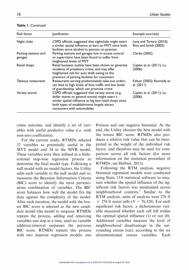
of overall street-level crime occurrence and/or MVT. Other risk factors were included atthe recommendation of Colorado SpringsPolice Department personnel, based upontheir knowledge of local crime conditions.This selection method helps ensure that thefactors included in the study are bothempirically driven and practically meaning-ful (see Table 1) (Kennedy et al., 2015).
Lastly, the analysis included neighbourhood-level data collected from the US CensusBureau’s American Community Survey5-year estimates (2009–2013).
Data were collected at the census tractlevel, which prior research has consistentlyused as an operationalisation of neighbour-hood (Griffiths and Chavez, 2004; Kubrinand Herting, 2003; Stucky et al., 2016), andare collectively identified as census variables.We included six separate census variables,all of which have been positively associatedwith crime occurrence in prior research: thepercentage of persons below the poverty line(Pratt and Cullen, 2005); racial heterogene-ity6 (Berg et al., 2012); geographic mobility:percentage of persons who lived at a differ-ent address the previous year (Bruce et al.,1998); educational attainment: percentage ofadults without a high school diploma orequivalent degree (Chainey, 2008); popula-tion density: persons per square mile(Osgood and Chambers, 2000; Sampson,1983); and the young male population: per-centage of persons that are male between theages of 15 and 24 (Kubrin and Herting,2003). Data were joined to a GIS layer ofcensus tracts in El Paso county, whichencompasses Colorado Springs, for the anal-ysis (N = 130).
Analytical strategy
In conducting Risk Terrain Modelling, weused the RTMDx Utility developed by theRutgers Center on Public Security (Caplanand Kennedy, 2013). RTMDx uses a precise
set of statistical tests to (1) choose the appro-priate operationalisation of each risk factor;(2) determine the appropriate model type(Poisson or negative binomial); and (3)determine the relative importance of risk fac-tors in influencing crime outcomes (Heffner,2013). For the analysis, Colorado Springswas modelled as a set of contiguous grids ofequally sized 276 ft 3 276 ft. cells (N =76,528), representing approximately one-halfof the average block length in the city, asmeasured within ArcGIS. RTMDx tests riskfactor influence through a penalised regres-sion model with crime counts (in this case,MVT or MVR) as the dependent variable.Various operationalisations of the aforemen-tioned risk factors are independent variables,with RTMDx measuring whether each rastercell is within a certain distance of the riskfactor (i.e. proximity) or in an area of highconcentration of the risk factor (i.e. density).Each risk factor was tested at three dis-tances: 1 block (552 ft), 2 blocks (1104 ft)and 3 blocks (1656 ft). Through this method,the 19 risk factors generated 84 independentvariables that were tested for significance.
Incorporating 84 covariates in a singlemodel may present problems with multiplecomparisons, in that we may detect spuriouscorrelation simply because of the number ofvariables tested. The penalised regressionmethod used by RTMDx alleviates potentialproblems with spurious correlation owing tomultiple comparisons by reducing the largeset of variables to a smaller set of variableswith non-zero coefficients. This is accom-plished through an elastic net method thatforms five stratified folds from the rastercells, balancing crime counts between thefolds. This balancing process is done toensure that there is some variance across thefolds to aid in the numeric stability of themodeling process. For each covariate,RTMDx then builds five simultaneous mod-els for each fold to rigorously test the influ-ence of each independent variable on the
8 Urban Studies
at JOHN JAY COLLEGE on August 24, 2016usj.sagepub.comDownloaded from

Table 1. Risk factor conceptualisation and justification.
Risk factor Justification Example source(s)
Bars Research has frequently found bars to generatestreet-level crime. Motor vehicles are likely to beparked near bars (and restaurants) in the eveninghours, creating opportunities for MVT
Levy and Tartaro (2010);Rice and Smith (2002)
Bowling centres CSPD identified bowling centres as a particular typeof entertainment venue that may generateopportunities for MVT. Environmentalcriminologists have referred to such crime-generating venues as social crime facilitators
Clarke and Eck (2005)
Commercial zoning Research has found commercial locations to be atheightened risk of MVT, presumably because of theconcentration of automobiles in such areas
Lu (2006)
Convenience stores Research has found that convenience stores andcorner grocery stores generate street-level crime inthe surrounding vicinity
Bernasco and Block(2011); Myers (2002)
Gas stations withconvenience stores
Research has shown gas stations to be associatedwith repeat MVT locations. CSPD officials furtherrecommended that we include only gas stationswith convenience stores given the uniqueopportunity structure at such gas stations (seefootnote 2)
Levy and Tartaro (2010)
Disorder-relatedcalls for service
Reviews of research find evidence that socialdisorder stimulates street-level crime, both directlyand via its impact on other aspects of community
Skogan (2015)
Foreclosedproperties
Foreclosures and general vacant housing have beenfound to generate the occurrence of crime,including MVT
Katz et al. (2013); Sureshand Tewksbury (2013)
Hotels and motels Prior research including both routine activity andSocial Disorganisation variables has found thepresence of a hotel or motel to be the mostpowerful predictor of MVT
Rice and Smith (2002)
Multi-family housingcomplexes
Large-scale multi-family dwellings have beenassociated with lower guardianship and highercriminal activity, including MVT. Victimisationsurveys suggest that people residing in single-familystructures are less likely to experience MVT thanpeople residing in multi-family structures
Lu (2006); Poyner (2006);Rice and Smith (2002)
Parks Research has found parks to be related topredatory crime, owing to their typically low levelsof guardianship
Groff and McCord (2011)
Sit-down restaurants Motor vehicles are likely to be parked nearrestaurants (and bars) during evening hours,creating opportunities for theft
Rice and Smith (2002)
Schools Research has found that schools increase propertycrime in the surrounding area
LaGrange (1999); Roncek(2000)
Liquor stores Research has found the presence of off-premiseliquor establishments to be associated withheightened occurrence of predatory crime
Bernasco and Block(2011); Snowden andPridemore (2013)
Malls Malls provide heightened levels of risk for MVTowing to the large-scale availability of parking andthe fact that patrons leave their vehicles unattendedfor extended periods of time
Clarke (2002); LaGrange(1999); Lu (2006)
(continued)
Piza et al. 9
at JOHN JAY COLLEGE on August 24, 2016usj.sagepub.comDownloaded from
crime outcome, and identify a set of vari-
ables with useful predictive value (i.e. with
non-zero coefficients).For the current study, RTMDx selected
32 variables as potentially useful in theMVT model and 34 in the MVR model.These variables were then utilised in a bidir-ectional step-wise regression process todetermine the final model type. Following anull model with no model factors, the Utilityadds each variable to the null model and re-measures the Bayesian Information Criteria(BIC) score to identify the most parsimo-nious combination of variables. The BICscore balances how well the model fits thedata against the complexity of the model.After each iteration, the model with the low-est BIC score is selected as the new candi-date model (the model to surpass). RTMDxrepeats the process, adding and removingvariables one step at a time, until no variableaddition/removal surpasses the previousBIC score. RTMDx repeats this processwith two stepwise regression models: one
Poisson and one negative binomial. At theend, the Utility chooses the best model withthe lowest BIC score. RTMDx also pro-duces a relative risk value that can be inter-preted as the weight of the individual riskfactor, and therefore may be used for com-parison across all risk factors (for moreinformation on the statistical procedure ofRTMDx, see Heffner, 2013).
Following the RTM analysis, negativebinomial regression models were conductedusing Stata 13.0 statistical software to mea-sure whether the spatial influence of the sig-nificant risk factors was maintained acrossneighbourhood contexts.7 Similar to theRTM analysis, units of analysis were 276 ft3 276 ft raster cells (N = 76,528). For eachsignificant risk factor, a dichotomous vari-able measured whether each cell fell withinthe optimal spatial influence (1) or not (0).Additional variables measure the level ofneighbourhood disadvantage in the sur-rounding census tract, according to the sixaforementioned census variables. Each
Table 1. Continued
Risk factor Justification Example source(s)
Night clubs CSPD officials suggested that nightclubs might exerta similar spatial influence as bars on MVT since bothfacilities serve alcohol to patrons on-premise
Levy and Tartaro (2010);Rice and Smith (2002)
Parking stations andgarages
Parking stations and garages low in access controlor supervision have been found to suffer fromheightened levels of MVT
Clarke (2002)
Retail shops Retail business outlets have been shown to generateincidents of predatory crime, and may offerheightened risk for auto theft owing to thepresence of parking facilities for customers
Caplan et al. (2011); Lu(2006)
Takeout restaurants Restaurants serving predominately take-out orderscan lead to high levels of foot traffic and low levelsof guardianship, which can promote crime
Felson (2002); Kennedy etal. (2011)
Variety stores CSPD officials suggested that variety stores (e.g.dollar stores or general stores) might exert asimilar spatial influence as big box retail shops sinceboth types of establishments largely attractconsumers with automobiles
Caplan et al. (2011); Lu(2006)
10 Urban Studies
at JOHN JAY COLLEGE on August 24, 2016usj.sagepub.comDownloaded from

census variable was re-coded so that thevalue in each census tract was identified asgreater than 1 standard deviation below themean (21), between 1 standard deviationbelow the mean and 1 standard deviationabove the mean (0), or greater than 1 stan-dard deviation above the mean (1). Wedecided to operationalise the census valuesin this manner to provide standardised mea-sures across variables. Table 2 displaysdescriptive statistics for the dichotomousRTM and re-coded census variables.
The dichotomous variable for each signif-icant risk factor was multiplied with eachre-coded census variable to create six inter-action terms: risk factor 3 racial
heterogeneity, risk factor 3 young malepopulation, risk factor 3 geographic mobi-lity, risk factor 3 no high school, risk fac-tor 3 population density, and risk factor3 poverty. Figure 2 provides a visual exam-ple of this process. This resulted in 42 inter-action terms in the MVT model and 60interaction terms in the MVR model. Forboth models, a spatial lag variable was cre-ated within the GeoDa spatial analysis soft-ware to control for the observed presence ofspatial autocorrelation.8 To measure thepresence of multicollinarity, we calculatedthe variance inflation factor (VIF) and asso-ciated tolerance (1/VIF) for each of theexploratory variables (Hamilton, 2013: 203).
Figure 2. Spatial influence and neighbourhood vulnerability maps.Note: In each of the maps, grid cells are the unit of analysis.
Piza et al. 11
at JOHN JAY COLLEGE on August 24, 2016usj.sagepub.comDownloaded from

Tab
le2.
Des
crip
tive
stat
istics
.
Var
iable
Moto
rVeh
icle
Thef
tm
odel
Moto
rVeh
icle
Rec
ove
rym
odel
Continuous
mea
sure
sO
rdin
alm
easu
res
(%)
Continuous
mea
sure
sO
rdin
alm
easu
res
(%)
Mea
n(S
D)
Min
(Max
)2
10
1M
ean
(SD
)M
in(M
ax)
21
01
Dep
endent
vari
able
:C
rim
ein
ciden
tco
unt
0.1
2(0
.13)
0 (6)
––
–0.1
2(0
.14)
0 (7)
––
–
Ris
kfa
ctors
:D
isord
erca
lls–
––
69,4
31
(90.
73)
7097
(9.2
7)
––
–70,1
05
(91.6
1)
6423
(8.3
9)
Fore
closu
res
––
–39,7
17
(51.
90)
36,8
11
(48.1
0)
––
–39,7
17
(51.9
0)
36,8
11
(48.1
0)
Multi-fa
mily
housi
ng
com
ple
xes
––
–40,6
24
(53.
08)
35,9
04
(46.9
2)
––
–40,6
24
(53.0
8)
35,9
04
(46.9
2)
Hote
ls&
mote
ls–
––
75,1
05
(98.
14)
1423
(1.8
6)
––
–75,1
05
(98.1
4)
1423
(1.8
6)
Sit-
dow
nre
stau
rants
––
–54,1
10
(70.
71)
22,4
18
(29.2
9)
––
–54,1
10
(70.7
1)
22,4
18
(29.2
9)
Par
ks–
––
31,5
35
(41.
21)
44,9
93
(58.7
9)
––
–31,5
35
(41.2
1)
44,9
93
(58.7
9)
Com
mer
cial
zonin
g–
––
52,4
79
(68.
57)
24,0
49
(31.4
3)
––
–52,4
79
(68.5
7)
24,0
49
(31.4
3)
Conv
enie
nce
store
s–
––
––
––
–74,3
32
(97.1
3)
2196
(2.8
7)
Gas
stat
ions
w/c
onv
enie
nce
store
s–
––
––
––
–72,4
79
(94.7
1)
4049
(5.2
9)
Schools
––
––
––
––
63,0
32
(82.3
6)
13,4
96
(17.6
4)
Soci
o-d
em
ogr
ap
hic
s:R
acia
lhet
eroge
nei
ty0.0
8(0
.04)
0.0
0(0
.16)
12,1
18
(15.8
3)
57,2
65
(74.
83)
7145
(9.3
4)
Sam
eas
Moto
rVeh
icle
Thef
tM
odel
Young
mal
epopula
tion
13.1
7(8
.03)
0 (98.
53)
0 (0)
69,9
37
(91.
39)
6591
(8.6
1)
ibid
.
(con
tinue
d)
12 Urban Studies
at JOHN JAY COLLEGE on August 24, 2016usj.sagepub.comDownloaded from
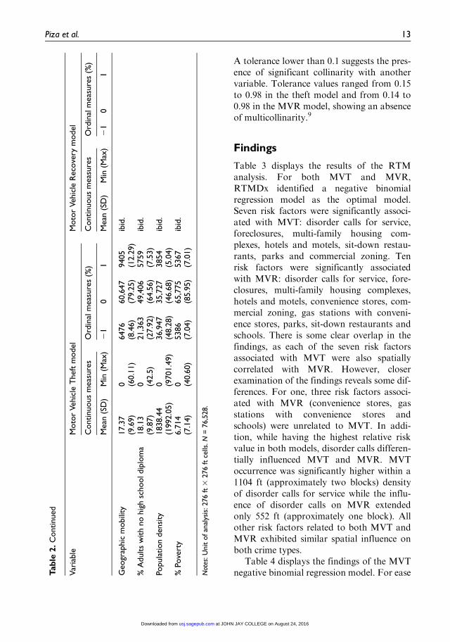
A tolerance lower than 0.1 suggests the pres-ence of significant collinarity with anothervariable. Tolerance values ranged from 0.15to 0.98 in the theft model and from 0.14 to0.98 in the MVR model, showing an absenceof multicollinarity.9
Findings
Table 3 displays the results of the RTManalysis. For both MVT and MVR,RTMDx identified a negative binomialregression model as the optimal model.Seven risk factors were significantly associ-ated with MVT: disorder calls for service,foreclosures, multi-family housing com-plexes, hotels and motels, sit-down restau-rants, parks and commercial zoning. Tenrisk factors were significantly associatedwith MVR: disorder calls for service, fore-closures, multi-family housing complexes,hotels and motels, convenience stores, com-mercial zoning, gas stations with conveni-ence stores, parks, sit-down restaurants andschools. There is some clear overlap in thefindings, as each of the seven risk factorsassociated with MVT were also spatiallycorrelated with MVR. However, closerexamination of the findings reveals some dif-ferences. For one, three risk factors associ-ated with MVR (convenience stores, gasstations with convenience stores andschools) were unrelated to MVT. In addi-tion, while having the highest relative riskvalue in both models, disorder calls differen-tially influenced MVT and MVR. MVToccurrence was significantly higher within a1104 ft (approximately two blocks) densityof disorder calls for service while the influ-ence of disorder calls on MVR extendedonly 552 ft (approximately one block). Allother risk factors related to both MVT andMVR exhibited similar spatial influence onboth crime types.
Table 4 displays the findings of the MVTnegative binomial regression model. For easeT
ab
le2.C
ontinued
Var
iable
Moto
rVeh
icle
Thef
tm
odel
Moto
rVeh
icle
Rec
ove
rym
odel
Continuous
mea
sure
sO
rdin
alm
easu
res
(%)
Continuous
mea
sure
sO
rdin
alm
easu
res
(%)
Mea
n(S
D)
Min
(Max
)2
10
1M
ean
(SD
)M
in(M
ax)
21
01
Geo
grap
hic
mobili
ty17.3
7(9
.69)
0 (60.
11)
6476
(8.4
6)
60,6
47
(79.
25)
9405
(12.2
9)
ibid
.
%A
dults
with
no
hig
hsc
hooldip
lom
a18.1
3(9
.87)
0 (42.
5)
21,3
63
(27.9
2)
49,4
06
(64.
56)
5759
(7.5
3)
ibid
.
Popula
tion
den
sity
1838.4
4(1
992.0
5)
0 (970
1.4
9)
36,9
47
(48.2
8)
35,7
27
(46.
68)
3854
(5.0
4)
ibid
.
%Po
vert
y6.7
14
(7.1
4)
0 (40.
60)
5386
(7.0
4)
65,7
75
(85.
95)
5367
(7.0
1)
ibid
.
Not
es:U
nit
ofan
alys
is:276
ft3
276
ftce
lls.N
=76,5
28.
Piza et al. 13
at JOHN JAY COLLEGE on August 24, 2016usj.sagepub.comDownloaded from

Tab
le3.
Ris
kfa
ctor
test
ing.
Ris
kFa
ctor
Moto
rVeh
icle
Thef
tM
oto
rVeh
icle
Rec
ove
ry
NO
p.S.
I.C
oef
.R
RV
Op.
S.I.
Coef
.R
RV
Inth
efin
alRT
MD
isord
erca
lls16,3
25
Den
s.1104
ft1.3
03.6
9D
ens.
552
ft1.5
94.8
8Fo
recl
osu
res
899
Pro
x.
1656
ft0.8
92.4
6Pro
x.
1656
ft0.7
52.1
1M
ulti-fa
mily
housi
ng
com
ple
xes
11,2
61
Pro
x.
1656
ft0.9
02.4
6Pro
x.
1656
ft0.6
51.9
2H
ote
ls&
mote
ls111
Pro
x.
552
ft0.6
41.9
0Pro
x.
552
ft0.6
31.8
8Si
t-dow
nre
stau
rants
550
Pro
x.
1656
ft0.6
11.8
5Pro
x.
1656
ft0.4
11.5
0Par
ks14,4
64
Pro
x.
1656
ft0.4
41.5
5Pro
x.
1656
ft0.4
81.6
1C
om
mer
cial
zonin
g13,4
85
Pro
x.
1656
ft0.3
11.3
7Pro
x.
1656
ft0.5
21.6
8C
onv
enie
nce
store
s77
––
––
Pro
x.
552
ft0.6
21.8
5G
asst
atio
ns
w/c
onv
enie
nce
store
s28
––
––
Pro
x.
1656
ft0.5
01.6
8Sc
hools
106
––
––
Pro
x.
1656
ft0.3
01.3
5In
terc
ept
(rat
e)–
––
26.5
6–
––
26.4
8–
Inte
rcep
t(o
verd
isper
sion)
––
–2
1.0
5–
–2
0.8
2–
Test
edbu
tno
tin
the
final
RTM
Bar
s111
––
––
––
––
Bow
ling
centr
es8
––
––
––
––
Liquor
store
s93
––
––
––
––
Mal
ls6
––
––
––
––
Nig
ht
clubs
15
––
––
––
––
Par
king
stat
ions
&ga
rage
s6
––
––
––
––
Ret
ailsh
ops
57
––
––
––
––
Take
out
rest
aura
nts
299
––
––
––
––
Var
iety
store
s21
––
––
––
––
Not
es:A
bbr
evia
tions
:O
p.,O
per
atio
nal
isat
ion;D
ens,
Den
sity
;Pro
x.,
Pro
xim
ity;
S.I.,
Spat
ialin
fluen
ce;C
oef
.,C
oef
ficie
nt;
RRV,
Rel
ativ
eri
skva
lue.
RT
MD
xonly
acce
pts
poin
tfil
esas
inputs
.M
ulti-fa
mily
housi
ng
com
ple
xes,
par
ksan
dco
mm
erci
alzo
ning
wer
epro
vided
aspoly
gons
and
conv
erte
dto
poly
gons
pri
or
toth
e
anal
ysis
.To
cond
uct
the
conv
ersi
on,re
sear
cher
sfir
stco
nver
ted
the
per
imet
erofea
chpoly
gon
toa
seri
esofpoin
tspla
ced
about
one
hal
fblo
ck(i.e
.276
ft)
from
each
oth
er.
Toco
nver
tth
ein
teri
or
ofth
epoly
gon,th
eve
ctor
was
first
conv
erte
dto
ara
ster
grid
with
cell
size
of276
ft.T
he
rast
erw
asth
enco
nver
ted
toa
poin
tfil
e,w
ith
each
rast
er
cell
centr
oid
repre
sente
das
asi
ngl
epoin
t.T
he
Nva
lues
inTa
ble
1ar
eth
enum
ber
ofpoin
tsin
put
into
RT
MD
x.T
he
poin
tsw
ere
crea
ted
from
the
follo
win
gnum
ber
of
poly
gon
feat
ure
s:459
multi-fa
mily
hous
ing
com
ple
xes,
26
com
mer
cial
zoni
ng
area
san
d530
par
ks.
14 Urban Studies
at JOHN JAY COLLEGE on August 24, 2016usj.sagepub.comDownloaded from
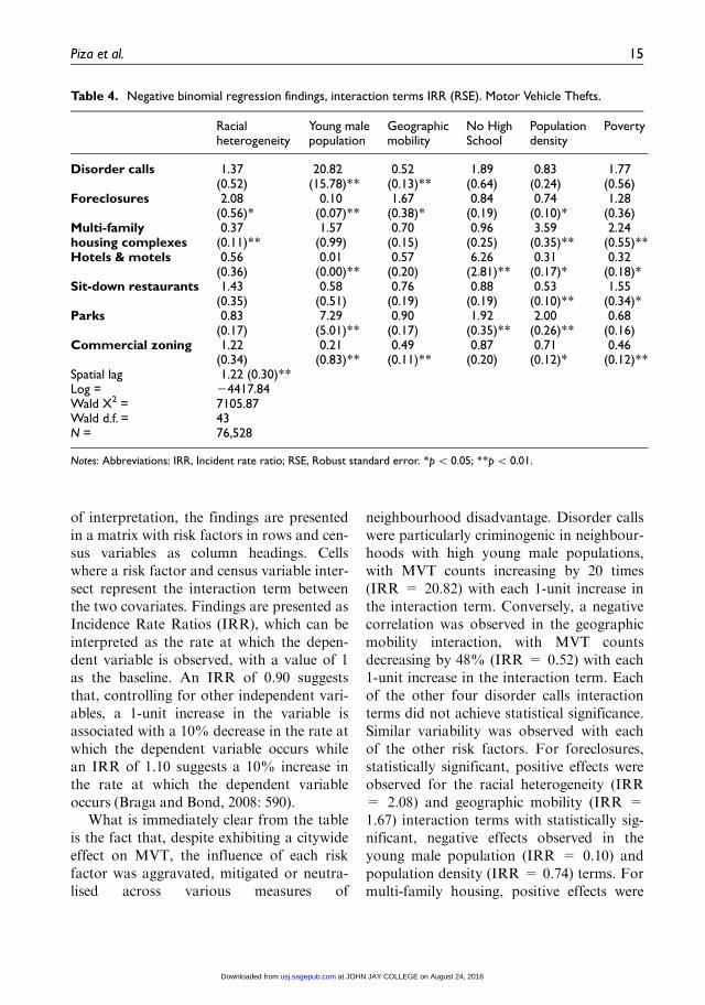
of interpretation, the findings are presentedin a matrix with risk factors in rows and cen-sus variables as column headings. Cellswhere a risk factor and census variable inter-sect represent the interaction term betweenthe two covariates. Findings are presented asIncidence Rate Ratios (IRR), which can beinterpreted as the rate at which the depen-dent variable is observed, with a value of 1as the baseline. An IRR of 0.90 suggeststhat, controlling for other independent vari-ables, a 1-unit increase in the variable isassociated with a 10% decrease in the rate atwhich the dependent variable occurs whilean IRR of 1.10 suggests a 10% increase inthe rate at which the dependent variableoccurs (Braga and Bond, 2008: 590).
What is immediately clear from the tableis the fact that, despite exhibiting a citywideeffect on MVT, the influence of each riskfactor was aggravated, mitigated or neutra-lised across various measures of
neighbourhood disadvantage. Disorder callswere particularly criminogenic in neighbour-hoods with high young male populations,with MVT counts increasing by 20 times(IRR = 20.82) with each 1-unit increase inthe interaction term. Conversely, a negativecorrelation was observed in the geographicmobility interaction, with MVT countsdecreasing by 48% (IRR = 0.52) with each1-unit increase in the interaction term. Eachof the other four disorder calls interactionterms did not achieve statistical significance.Similar variability was observed with eachof the other risk factors. For foreclosures,statistically significant, positive effects wereobserved for the racial heterogeneity (IRR= 2.08) and geographic mobility (IRR =1.67) interaction terms with statistically sig-nificant, negative effects observed in theyoung male population (IRR = 0.10) andpopulation density (IRR = 0.74) terms. Formulti-family housing, positive effects were
Table 4. Negative binomial regression findings, interaction terms IRR (RSE). Motor Vehicle Thefts.
Racialheterogeneity
Young malepopulation
Geographicmobility
No HighSchool
Populationdensity
Poverty
Disorder calls 1.37(0.52)
20.82(15.78)**
0.52(0.13)**
1.89(0.64)
0.83(0.24)
1.77(0.56)
Foreclosures 2.08(0.56)*
0.10(0.07)**
1.67(0.38)*
0.84(0.19)
0.74(0.10)*
1.28(0.36)
Multi-familyhousing complexes
0.37(0.11)**
1.57(0.99)
0.70(0.15)
0.96(0.25)
3.59(0.35)**
2.24(0.55)**
Hotels & motels 0.56(0.36)
0.01(0.00)**
0.57(0.20)
6.26(2.81)**
0.31(0.17)*
0.32(0.18)*
Sit-down restaurants 1.43(0.35)
0.58(0.51)
0.76(0.19)
0.88(0.19)
0.53(0.10)**
1.55(0.34)*
Parks 0.83(0.17)
7.29(5.01)**
0.90(0.17)
1.92(0.35)**
2.00(0.26)**
0.68(0.16)
Commercial zoning 1.22(0.34)
0.21(0.83)**
0.49(0.11)**
0.87(0.20)
0.71(0.12)*
0.46(0.12)**
Spatial lag 1.22 (0.30)**Log = 24417.84Wald X2 = 7105.87Wald d.f. = 43N = 76,528
Notes: Abbreviations: IRR, Incident rate ratio; RSE, Robust standard error. *p \ 0.05; **p \ 0.01.
Piza et al. 15
at JOHN JAY COLLEGE on August 24, 2016usj.sagepub.comDownloaded from

observed in the population density (IRR =3.59) and poverty (IRR = 2.24) interactionterms, with increases in the racial heteroge-neity term associated with decreased MVT(IRR = 0.37). For hotels & motels, each 1-unit increase in the youth population termwas associated with an extremely sizable (i.e.99%) reduction in MVT (IRR = 0.01), withthe poverty (IRR = 0.32) and populationdensity (IRR = 0.31) terms also exhibitingnegative relationships. Each 1-unit increasein the no high school interaction term wasassociated with an over six-fold increase inMVT (IRR= 6 .26). Only two of the sit-down restaurant interaction terms achievedstatistical significance, with each 1-unitincrease in the population density term asso-ciated with a 47% reduction in MVT (IRR= 0.53) and each 1-unit increase in the pov-erty term associated with a 55% increase(IRR = 1.55). The three statistically signifi-cant parks interaction terms were associatedwith increased levels of MVT. Each 1-unitincrease in the no high school (IRR = 1.92)and population density (IRR = 2.00) termswas associated with approximately a dou-bling of MVT while a 1-unit increase in theyoung male population term (IRR = 7.29)was associated with an over seven-foldincrease in MVT. Each of the four signifi-cant commercial zoning interaction termswas associated with decreased levels ofMVT: young male population (IRR =0.21), geographic mobility (IRR = 0.49),population density (IRR = 0.71) and pov-erty (IRR = 0.46).
Table 5 displays the findings of the MVRnegative binomial regression model. Similarto the MVT model, variability was observedfor each risk factor. Four of the disordercalls terms were statistically significant forMVR, as compared with two in the MVTmodel. The terms for young male population(IRR = 12.77) and geographic mobility(IRR = 0.36) were associated with increasedand decreased MVR, respectively, similar to
their influence in the MVT model. One-unitincreases in the no high school (IRR = 3.03)and poverty (IRR = 2.24) terms were eachassociated with MVR rate increases. Only asingle foreclosure term achieved statisticalsignificance, with each 1-unit increase in thepopulation density term associated with a25% reduction in MVR (IRR = 0.75),nearly identical to the effect observed in theMVT model. Two of the multi-family hous-ing complex interaction terms achieved sta-tistical significance, with both the populationdensity (IRR = 3.20) and poverty (IRR =1.86) terms associated with increased MVR.Both of these terms exerted a similar effect inthe MVT model. The racial heterogeneityterm, significant in the MVT model, wasinsignificant for MVR. Two of the hotels &motels terms were statistically significant.Each 1-unit increase in the young male pop-ulation term was associated with a 99%reduction in the rate of MVR, identical to itsobserved effect in the MVT model. The geo-graphic mobility term, insignificant in theMVT model, was associated with reductionsin MVR (IRR = 0.47). For sit-down restau-rants, the population density term was asso-ciated with reduced levels of MVR (IRR =0.48), similar to the MVT findings. Theother significant term in the MVT model(poverty) was insignificant for MVR. Thethree parks terms associated with MVTincreases were similarly associated withMVR: young male population (IRR =5.14), no high school diploma (IRR = 3.22),and population density (IRR = 2.81). Theracial heterogeneity term, insignificant in theMVT model, was associated with decreasedMVR (IRR = 0.46). For commercial zon-ing, the four significant terms exhibited simi-lar effects on MVT as MVR: young malepopulation (IRR = 0.10), geographic mobi-lity (IRR = 0.65), population density (IRR= 0.58), and poverty (IRR= 0.48).
Three risk factors associated with MVRwere not associated with MVT (convenience
16 Urban Studies
at JOHN JAY COLLEGE on August 24, 2016usj.sagepub.comDownloaded from

stores, gas stations with convenience stores,and schools) so a comparison of interactionterms across models is not possible. For con-venience stores, three interaction termsachieved statistical significance. Each 1-unit
increase in the poverty term was associated
with a more than tripling of the MVR rate
(IRR = 3.41) while the young male popula-
tion (IRR = 0.04) and geographic mobility
(IRR = 0.61) terms were associated with a
reduction in MVR. For gas stations with
convenience stores, each 1-unit increase in
the racial heterogeneity term was associated
with a tripling of MVR (IRR = 3.00) while
each 1-unit increase in the young male popu-
lation term was associated with a 99%
reduction of MVR (IRR = 0.01). Only a
single interaction term was significant for
schools, with each 1-unit increase in popula-
tion density associated with a 63% reduction
of MVR (IRR = 0.37).
Discussion and conclusion
This study contributed to the literature intwo primary ways. First, we identified thespatial correlates of both MVT and MVR,two crime types that have appeared spar-ingly in the geospatial literature. The topfour risk factors, in terms of relative riskvalue, were identical for MVT and MVR:disorder related calls for service, foreclo-sures, multi-family housing units, and hotelsand motels. In addition, each of the risk
Table 5. Negative binomial regression findings, interaction terms IRR (RSE). Motor Vehicle Recoveries.
Racialheterogeneity
Young malepopulation
Geographicmobility
No HighSchool
Populationdensity
Poverty
Disorder calls 0.95(0.36)
12.77(12.09)**
0.36(0.08)**
3.03(1.18)**
1.00(0.29)
2.24(0.73)*
Foreclosures 1.45(0.35)
0.32(0.29)
0.99(0.21)
0.75(0.16)
0.75(0.11)*
1.10(0.31)
Multi-familyhousing complexes
0.82(0.25)
1.51(1.09)
0.79(0.17)
0.67(0.22)
3.20(0.31)**
1.86(0.53)*
Hotels & motels 0.52(0.55)
0.01(0.00)**
0.47(0.15)*
3.09(2.57)
0.42(0.32)
0.44(0.32)
Sit-down restaurants 1.22(0.36)
1.06(0.87)
0.95(0.22)
1.15(0.34)
0.48(0.09)**
1.27(0.33)
Parks 0.46(0.11)**
5.14(4.29)*
0.77(0.16)
3.22(0.90)**
2.81(0.48)**
1.19(0.34)
Commercial zoning 1.62(0.43)
0.10(0.05)**
0.65(0.12)**
0.82(0.18)
0.58(0.11)**
0.48(0.12)**
Convenience stores 0.89(0.60)
0.04(0.01)**
0.61(0.15)*
0.27(0.19)
0.68(0.36)
3.41(2.08)*
Gas stations withconvenience stores
3.00(1.47)*
0.01(0.00)**
0.80(0.22)
0.71(0.52)
1.16(0.40)
0.59(0.22)
Schools 1.54(0.47)
0.36(0.29)
0.90(0.18)
0.90(0.22)
0.37(0.08)**
1.37(0.33)
Spatial lag 1.18 (0.03)**Log = 24150.96Wald X2 = 18,398Wald d.f. = 61N = 76,528
Notes: Abbreviations: IRR, Incident rate ratio; RSE, Robust standard error. *p \ 0.05; **p \ 0.01.
Piza et al. 17
at JOHN JAY COLLEGE on August 24, 2016usj.sagepub.comDownloaded from

factors significant for MVT were also signifi-cant for MVR (disorder related calls for ser-vice, foreclosures, multi-family housingcomplexes, hotels and motels, sit-down res-taurants, parks and commercial zoning). Anadditional three risk factors (conveniencestores, gas stations w/convenience stores andschools) influenced the occurrence of MVR,but not MVT.
The nature of the significant risk factorssuggests the importance of deniability, whichSt Jean (2007) describes as the ability todeny that one is present in an area for crimi-nal purposes. Prior research has identifieddeniability as an important factor for offen-ders looking to ‘blend-in’ at a particular areafor extended periods of time, such as drugsellers (Piza and Sytsma, 2016; St Jean,2007). However, research suggests thatdeniability is also important for offenderslooking to quickly flee an area, such asarmed robbers (St Jean, 2007). The currentstudy findings suggest deniability may be animportant consideration for motor vehiclethieves. Outside of disorder related calls forservice, all of the significant risk factors arelegitimate features of land usage, rather thancenters of illicit behaviour. In the lexicon ofEnvironmental Criminology, these risk fac-tors represent crime generators: places towhich large numbers of people are attractedfor reasons unrelated to criminal motivationbut that nonetheless offer increased opportu-nities for crime (Clarke and Eck, 2005: 17).Searching for targets in such areas allowsoffenders to maintain an inconspicuous pres-ence because other persons are frequentingthe area for legitimate reasons. Deniabilityseems to be even more important for MVR,given the nature of the three risk factorsrelated to MVR but not MVT. Conveniencestores and gas stations with conveniencestores provide thieves an opportunity topark a motor vehicle in an area where manyother motorists do the same. In such anenvironment, an offender not returning to
the vehicle is unlikely to be noticed by anyon-lookers. Areas around schools similarlyattract people who must leave their vehiclesunattended for extended periods.
We further found the effect of each signif-icant risk factor to be heterogeneous acrossneighbourhood context. This suggests thatthe convergence of particular spatial andneighbourhood-level factors may maintainor heighten criminogenic effects, while theconvergence of other factors may result in anull or mitigating effect. Moreover, certaininteraction terms were statistically significantin one model but not the other. This suggeststhat the interaction of risk factor spatialinfluence and neighbourhood disadvantagedifferently influence MVT and MVR.
The significance of the interaction termssupports the notion of EnvironmentalCriminology and Social Disorganisation ascomplementary, rather than competing, the-oretical perspectives. Despite the tendencyfor scholars to consider these theories ascontrasting, their conceptual frameworksoverlap. In particular, both place premiumimportance on the notion of informal socialcontrol (Bossen and Hipp, 2015: 400). SocialDisorganisation scholars argue that collec-tive efficacy is maintained through informalmechanisms, such as the ‘monitoring ofspontaneous play groups among children, awillingness to intervene to prevent acts suchas truancy and street-corner ‘‘hanging’’ byteenage peer groups, and the confrontationof persons who are exploiting or disturbingpublic space’ (Sampson et al., 1997).Environmental criminologists emphasise therole of intimate handlers and place mangersin exerting informal control over potentialoffenders within neighbourhoods (Eck,1994; Felson, 1995). Intimate handlers andplace managers often include the same enti-ties involved the development of collectiveefficacy, such as neighbourhood residents,business owners, apartment mangers andstreet pedestrians.
18 Urban Studies
at JOHN JAY COLLEGE on August 24, 2016usj.sagepub.comDownloaded from

Findings in the current study suggestan interaction between EnvironmentalCriminology and Social Disorganisationmechanisms. For example, the Risk TerrainModel found foreclosures to be related toincreased levels of both MVT and MVR ona city wide basis. However, foreclosureswithin areas of high population density weresignificantly associated with reduced countsof both MVT and MVR. A potential expla-nation may be that, while foreclosures trans-late to the removal of homeowners, theresidents most commonly associated withstability and investment (Immergluck andSmith, 2006; Katz et al., 2013), areas withhigh population densities may provide thenecessary guardians to prevent high levels ofMVT and MVR. In addition, the interactionbetween disorder calls and young male pop-ulation generated the highest IRR values forboth MVT and MVR. This suggests thatdisorder calls, criminogenic on their own,present maximum influence in areas wherethe size of the young male population chal-lenges the formation of collective efficacy.Theorising the underlying mechanism ofeach statistically significant interaction termis beyond the scope of this paper, given thelarge number of terms. Rather, we presentour findings as an illustration of the utilityof jointly considering micro-level risk factorsand neighbourhood-level measures in crime-and-place research. We recommend thatfuture research continue to explore the jointutility of these perspectives.
The findings also have implications forthe Policing field. While crime hot spotshave been used to identify targets for policeresources, crime forecasting techniques suchas Risk Terrain Modelling can help furtherrefine target areas (Caplan et al., 2013;Kennedy et al., 2011) while simultaneouslyidentifying criminogenic spatial features thatcrime prevention activities should target(Caplan et al., 2015; Kennedy et al., 2015).
The current study suggests that testing theinteraction effects between risk factors andneighbourhood dynamics may help to fur-ther focus crime prevention responses. Forexample, while foreclosures exhibited a city-wide effect on MVT, police may want toprioritise foreclosures in neighbours withhigh levels of racial heterogeneity and geo-graphic mobility, since crime risk was heigh-tened in these contexts. For MVR, officialsshould consider diverting crime preventionresources away from foreclosures in neigh-bourhoods with high population densities, sincethis context was actually associated withdecreased levels of crime. This suggests a two-step analytical procedure, the first step identify-ing the significant spatial risk factors and thesecond step measuring precise neighbourhoodcharacteristics that aggravate or mitigate thecriminogenic influence of said risk factors.While we focused on Motor Vehicle Crime inthe current study, such an approach can be usedto address any crime type.
Despite these implications, this study, likemost others, suffers from specific limitationsthat should be mentioned. Officiallyreported crime data is always subjected toreporting bias as not all crimes get reportedto the police. While MVT seemingly is notinfluenced by reporting bias as much asother offences, as 91.1% of completedMVTs are reported to police (BJS, 2015),reporting frequency of MVR is less clear.Regarding the RTM analysis, while we madeevery effort to include an exhaustive set ofrisk factors in the analysis, we were limitedto what was obtainable via available datasources. It is possible that pertinent, andinformative, spatial risk factors wereexcluded. In addition, while commonly usedas proxies for neighbourhoods, census tractsmay not accurately reflect resident percep-tions of community. Basta et al. (2010)found that respondents’ hand-drawn mapsof their neighbourhoods did not correspond
Piza et al. 19
at JOHN JAY COLLEGE on August 24, 2016usj.sagepub.comDownloaded from

with administrative boundaries such as cen-sus tracts, and that respondents living in thesame area had much different conceptions oftheir neighbourhoods. The reader should beaware of potential issues with face validity.Lastly, we alert the reader to the differingspatial scales of the data used to create theinteraction terms. All spatial risk factorswere operationalised at the micro-level (gridcell), with neighbourhood disadvantage mea-sured at the meso-level (census tract). Thisapproach mirrors the methodology of priorcrime-and-place research, with scholarssimultaneously incorporating EnvironmentalCriminology and Social Disorganisation per-spectives forced to use variables measured atdifferent scales (e.g. Braga et al., 2012;Drawve et al., 2016; Rice and Smith, 2002;Taniguchi and Salvatore, 2012). This is dueto the fact that socio demographic variablesare primarily collected by census bureaus,with pre-defined administrative areas (e.g.census tracts) as units of analysis. Whileresearch incorporating such measures hasgreatly contributed to the crime-and-place lit-erature, we echo recent calls for the improvedmeasurement of social disorganisation at themicro-level (Braga and Clarke, 2014;Weisburd et al., 2014), which would bettermatch the scale used to analyse crime andspatial risk factors. Future research shouldseek to address these study limitations.
Acknowledgements
The authors thank Molly Miles and AndrewDukes of the Colorado Springs PoliceDepartment for their support and assistancethroughout the project. An early version of thispaper was presented at the 2014 AmericanSociety of Criminology annual meeting. Wethank those in attendance for their insightfulquestions and feedback.
Funding
This research was supported by the NationalInstitute of Justice, grant #2012-IJ-CX-0038.
Notes
1. The use of a concise time frame means thatany stolen vehicle recovered after 31 October2013 is falsely classified as a permanentMVT, and thus not included in the currentstudy. However, prior research suggests thatstolen motor vehicles are typically recoveredwithin a week (Roberts, 2012). Qualitativeresearch on motor vehicle thieves suggeststhat the recovery time is accelerated in certaincases, with many offenders reporting thatthey abandon newer vehicles within two daysbecause of increased risk of detection (Jacobs
and Cherbonneau, 2014). Indeed, prior studieshave acknowledged the inability to account forMVR outside of the study period as a threat tovalidity (e.g. Roberts and Block, 2012; Sureshand Tewksbury, 2013). Therefore, we feel thatthe presence of false positives is minimised inour sample, and commensurate with that ofprior research on MVT.
2. The disorder calls for service include variousincidents considered as social disorder in theliterature: disorderly conduct, public intoxica-tion, loitering, noise complaints, aggressivepanhandling and trespassing.
3. After consulting with CSPD officials, wedecided to not include gas stations in theirentirety. This is because drivers do not typi-cally leave their vehicles unattended at gasstations. Therefore, the seizing of a motorvehicle in these locations would be classifiedas a robbery (with the vehicle being forcefullytaken from the victim) rather than a theft(with the vehicle being taken while not in thepresence of the victim). Gas stations that alsocontain convenience stores, conversely, haveparking areas for customers to leave theirvehicles. Since vehicles are unattended in suchcircumstances, their loss is classified as amotor vehicle theft.
4. Bars, commercial zoning, disorder relatedcalls for service, multi-family housing com-plexes, parks, sit-down restaurants, schools,liquor stores, malls, night clubs and takeoutrestaurants.
5. Bowling centres, convenience stores, foreclosedproperties, hotels & motels, gas stations withconvenience stores, parking stations & garages,retail shops and variety stores.
20 Urban Studies
at JOHN JAY COLLEGE on August 24, 2016usj.sagepub.comDownloaded from
6. Racial heterogeneity was calculated via thefollowing formula: [(%White, non-Hispanic *%non-white, non-Hispanic)+ (%black, non-Hispanic * %non-black, non-Hispanic)+(%Asian, non-Hispanic * %non-Asian, non-Hispanic)+ (%Hispanic * %non-Hispanic)]/4.
7. While RTMDx identified the best model forthe RTM analysis as a negative binomialregression, we manually diagnosed the datadistribution for the follow-up analysis since adifferent set of covariates (the interactionterms) were used as explanatory variables.
First, a Kolmogorov-Smirnov test confirmedthat both MVT (D = 43.87, p \ 0.01) andMVR (D = 48.50, p \ 0.01) had distribu-tions vastly different from a normal distribu-tion. Second, X2 goodness-of-fit testsconducted after exploratory Poisson regres-sion models confirmed that both MVT (X2
= 105,538.40, p \ 0.01) and MVR (X2 =143,249.10, p \ 0.01) were distributed as neg-ative binomial processes.
8. The inclusion of a spatial lag variable followsthe approach of prior research measuring theeffect of crime generators and attractors (e.g.Ashby and Bowers, 2015; Bernasco and Block,2011; Moreto et al., 2014). First order QueenContinuity was used in the creation of the spa-tial lag variables. Moran’s I was 0.06 (p =0.001) for MVT and 0.11 (p= 0.001) for MVR.Moran’s I statistics were calculated in GeoDa.
9. Owing to space constraints, VIF results arenot presented in text, but are available fromthe lead author upon request.
References
Andresen M (2014) Environmental Criminology.
Evolution, Theory, and Practice. London:
Routledge.Ashby M and Bowers K (2015) Concentrations of
railway metal theft and the locations of scrap-
metal dealers. Applied Geography 63: 283–291.Basta L, Richmond T and Wiebe D (2010) Neigh-
borhoods, daily activities, and measuring
health risks experienced in urban environ-
ments. Social Science & Medicine 71(11):
1943–1950.Berg M, Stewart E, Brunson R, et al. (2012)
Neighborhood cultural heterogeneity and
adolescent violence. Journal of Quantitative
Criminology 28(3): 411–435.Bernasco W and Block R (2011) Robberies in
Chicago: A block-level analysis of the influ-ence of crime generators, crime attractors, and
offender anchor points. Journal of Research in
Crime and Delinquency 48(1): 33–57.Boessen A and Hipp J (2015) Close-ups and the
scale of ecology: Land uses and the geography
of social context and crime. Criminology 53(3):399–426.
Braga A and Bond B (2008) Policing crime and
disorder hot spots. A randomized controlledtrial. Criminology 46(3): 577–607.
Braga A and Clarke R (2014) Explaining high-risk concentrations of crime in the city: Social
disorganization, crime opportunities, andimportant next steps. Journal of Research in
Crime and Delinquency 51(4): 480–498.Braga A, Hureau D and Papa Christos A (2012)
An ex post facto evaluation framework forplace-based police interventions. Evaluation
Review 35(6): 592–626.Brantingham PL and Brantingham PJ (1993)
Environment, routine, and situation: Towarda pattern theory of crime. In: Clarke RV and
Felson M (eds) Routine Activity and Rational
Choice. New Brunswick, NJ: Transaction pub-
lishers, Volume 5, pp. 259–294.Bruce M, Roscigno V and McCall P (1998) Struc-
ture, context, and agency in the reproductionof black-on-black violence. Theoretical Crim-
inology 2(1): 29–55.Bureau of Justice Statistics (BJS) (2011) Criminal
Victimization in the United States, 2008. Washing-
ton, DC: United States Department of Justice.Bureau of Justice Statistics (BJS) (2015) Criminal
Victimization in the United States, 2014.Washington, DC: United States Department
of Justice.Caplan J (2011). Mapping the spatial influence of
crime correlates: A comparison of operationa-lization schemes and implications for crime
analysis and criminal justice practice. City-
scape 13(3): 57–83.Caplan J and Kennedy L (2013). Risk Terrain
Modeling Diagnostics Utility (Version 1.0).Newark, NJ: Rutgers Center on Public Secu-rity. Available at: http://rutgerscps.weebly.
com/software.html.
Piza et al. 21
at JOHN JAY COLLEGE on August 24, 2016usj.sagepub.comDownloaded from

Caplan J, Kennedy L, Barnum J, et al. (2015)
Risk terrain modeling for spatial risk assess-
ment. Cityscape: A Journal of Policy Develop-
ment and Research 17(1): 7–16.Caplan J, Kennedy L and Miller J (2011) Risk
terrain modeling: Brokering criminological
theory and GIS methods for crime forecasting.
Justice Quarterly 28(2): 360–381.Caplan J, Kennedy L and Piza E (2013) Joint util-
ity of event dependent and contextual crime
analysis techniques for violent crime forecast-
ing. Crime and Delinquency 59(2): 243–270.Chainey S (2008) Identifying priority neighbor-
hoods using the vulnerable localities index.
Policing: A Journal of Policy and Practice 2(2):
196–209.Clarke R (2002) Thefts Of and From Cars in Park-
ing Facilities. Problem-Oriented Guides for
Police. Guide No. 10. Washington, DC: US
Department of Justice, Office of Community
Oriented Policing Services.Clarke R and Cornish D (1985) Modeling offen-
ders’ decisions: A framework for research and
policy. In: Tonry M and Norris M (eds) Crime
and Justice: An Annual Review of Research,
Vol. 6. Chicago, IL: University of Chicago
Press, pp. 147–186.Clarke R and Eck J (2005) Crime Analysis for
Problem Solvers in 60 Small Steps. Washing-
ton, DC: U.S. Department of Justice Office of
Community Oriented Policing Services.Clarke R and Harris P (1992) Auto theft and its
prevention. In: Tonry M (ed.) Crime and Jus-
tice: A Review of Research. Chicago, IL: Uni-
versity of Chicago Press, Volume 16, pp. 1–54.Cohen L and Felson M (1979) Social change and
crime rate trends: A routine activity approach.
American Sociological Review 44(4): 588–605.Copes H (1999) Routine activities and motor
vehicle theft: A crime specific approach. Jour-
nal of Crime and Justice 22(2): 125–146.Cornish D (1994) The procedural analysis of
offending and its relevance for situational pre-
vention. In: Clarke R (ed.) Crime Prevention
Studies. Monsey, NY: Criminal Justice Press,
Volume 3, pp. 151–196.Cornish D and Clarke R (1986) The Reasoning
Criminal: Rational Choice Perspectives on
Offending. New York: Springer-Verlag.
Drawve G (2016) A metric comparison of predic-
tive hot spot techniques and RTM. Justice
Quarterly 33(3): 369–397.Drawve G, Thomas S and Walker J (2016) Bring-
ing the physical environment back into neigh-
borhood research: The utility of RTM for
developing an aggregate neighborhood risk of
crime measure. Journal of Criminal Justice
44(1): 21–29.Eck J (1994) Drug markets and drug places: A
case-control study of the spatial structure of
illicit drug dealing. Doctoral Dissertation.
College Park, MD: University of Maryland.Eck J, Clarke R and Guerette R (2007) Risky
facilities: Crime concentration in homoge-
neous sets of establishments and facilities. In:
Farrel G, Bowers K, Johnson S and et al. (eds)
Imagination for Crime Prevention. Essays in
Honour of Ken Pease. Crime Prevention Stud-
ies. Monsey, NY: Criminal Justice Press, 21,
pp. 225–264.Federal Bureau of Investigation (FBI) (2015)
Crime in the United States 2014. Washington,
DC: US Department of Justice, Federal
Bureau of Investigation.Felson M (1995) Those who discourage crime.
Crime and Place 4: 53–66.Felson M (2002) Crime and Everyday Life. 3rd
Edition. Thousand Oaks, CA; London; New
Delhi: SAGE Publications.Griffiths E and Chavez J (2004) Communities,
street guns and homicide trajectories in Chi-
cago, 1980–1995. Merging methods for exam-
ining homicide trends across space and time.
Criminology 42(4): 941–978.Groff E and La Vigne N (2001) Mapping an
opportunity surface of residential burglary.
Journal of Research in Crime and Delinquency
38(3): 257–278.Groff E and Lockwood B (2014) Criminogenic
facilities and crime across street segments in Phi-
ladelphia: Uncovering evidence about the spatial
extent of facility influence. Journal of Research in
Crime and Delinquency 51(3): 277–314.Groff E and McCord E (2011) The role of neigh-
borhood parks as crime generators. Security
Journal 25(1): 1–24.Grubesic T, Mack E and Kaylen M (2012) Com-
parative modeling approaches for
22 Urban Studies
at JOHN JAY COLLEGE on August 24, 2016usj.sagepub.comDownloaded from
understanding urban violence. Social Science
Research 41(1): 92–109.Hamilton L (2013) Statistics with STATA.
Updated for Version 12. Boston, MA: Cengage
Brooks/Cole.Heffner J (2013) Statistics of the RTMDx utility.
In: Caplan J, Kennedy L and Piza E (eds) Risk
Terrain Modeling Diagnostics (RTMDx) Util-
ity User Manual (Version 1). Newark, NJ:
Rutgers Center on Public Security, pp. 26–34.Immergluck D and Smith G (2006) The impact of
single-family mortgage foreclosures on neigh-
borhood crime.Housing Studies 21(6): 851–866.Jacobs B and Cherbonneau M (2014) Auto theft
and restrictive deterrence. Justice Quarterly
31(2): 344–367.Katz C, Wallace D and Hedberg E (2013) A
longitudinal assessment of the impact of foreclo-
sure on neighborhood crime. Journal of Research
in Crime and Delinquency 50(3): 359–389.Kennedy L, Caplan J and Piza E (2011) Risk clus-
ters, hotspots, and spatial intelligence: Risk
terrain modeling as an algorithm for police
resource allocation strategies. Journal of Quan-
titative Criminology 27(3): 339–362.Kennedy L, Caplan J, Piza E, et al. (2015) Vul-
nerability and exposure to crime: Applying
risk terrain modeling to the study of assault in
Chicago. Applied Spatial Analysis and Policy.
Epub ahead of print 27 August 2015. DOI:
10.1007/s12061–015–9165-z.Kubrin C and Herting J (2003) Neighborhood
correlates of homicide trends: An analysis
using growth-curve modeling. Sociological
Quarterly 44(3): 329–350.LaGrange T (1999) The impact of neighborhoods,
schools, and malls on the spatial distribution
of property damage. Journal of Research in
Crime and Delinquency 36(4): 393–422.Levy M and Tartaro C (2010) Auto theft: A site-
survey and analysis of environmental crime
factors in Atlantic City, NJ. Security Journal
23(2): 75–94.Lilly J, Cullen F and Ball R (2011) Criminological
Theory. Context and Consequences. 5th Edi-
tion. Thousand Oaks, CA: Sage.Lockwood B (2012) The presence and nature of a
near-repeat pattern of motor vehicle theft.
Security Journal 25(1): 38–56.
Lu Y (2006) Spatial choice of auto thefts in an
urban environment. Security Journal 19(3):
143–166.Maguire E, Uchida C and Hassell K (2015) Prob-
lem-oriented policing in Colorado Springs: A
content analysis of 753 cases. Crime & Delin-
quency 61(1): 71–95.Maxfield M (2004) Introduction. In: Maxfield M
and Clarke R (eds) Understanding and Prevent-
ing Car Theft. Crime Prevention Studies, Vol-
ume 17. Monsey, NY: Criminal Justice Press.Morenoff J, Sampson R and Raudenbush S
(2001) Neighborhood inequality, collective
efficacy, and the spatial dynamics of urban
violence. Criminology 39(3): 517–559.Moreto W, Piza E and Caplan J (2014) A plague
on both your houses? Risks, repeats, and
reconsiderations of urban residential burglary.
Justice Quarterly 31(6): 1102–1126.Myers P (2002) The management of identity in
bodegas: Stigma and microeconomics in
Brooklyn. Journal of Ethnicity in Substance
Abuse 1(3): 75–92.Osgood D and Chambers J (2000) Social disorga-
nization outside the metropolis: An analysis of
rural youth violence. Criminology 38(1): 81–115.Piza E and Sytsma V (2016) Exploring the defen-
sive actions of drug sellers in open-air mar-
kets: A systematic social observation. Journal
of Research in Crime and Delinquency 53(1):
36–65.Poyner B (2006) Crime-free Housing in the 21st
Century. Jill Dando Institute of Crime Science,
University College of London. London: Brook
House Publishing.Pratt T and Cullen F (2005) Assessing macro-level
predictors and theories of crime: A meta-anal-
ysis. Crime and Justice 32: 373–450.Ratcliffe J (2012) The spatial extent of crimino-
genic places. A changepoint regression of vio-
lence around bars. Geographical Analysis
44(4): 302–320.Rice K and Smith W (2002) Socioecological mod-
els of automotive thefts: Integrating routine
activity and social disorganization approaches.
Journal of Research in Crime and Delinquency
39(3): 304–336.Roberts A (2012) Motor vehicle recovery: A mul-
tilevel event history analysis of NIBRS data.
Piza et al. 23
at JOHN JAY COLLEGE on August 24, 2016usj.sagepub.comDownloaded from

Journal of Research in Crime and Delinquency
49(3): 444–467.Roberts A and Block S (2012) Explaining tempo-
rary and permanent motor vehicle theft ratesin the United States. A crime-specificapproach. Journal of Research in Crime and
Delinquency 50(3): 445–471.Roncek D (2000) Schools and crime. In: Gold-
smith V, McGuire P and Mollenkopf J, et al.(eds) Analyzing Crime Patterns: Frontiers of
Practice. Thousand Oaks, CA: SAGE Publica-tions, pp. 153–165.
Sampson R (1983). Structural density and crimi-nal victimization. Criminology 21(2): 276–293.
Sampson R and Groves W (1989) Communitystructure and crime: Testing social disorgani-zation theory. American Journal of Sociology
94(4): 774–802.Sampson R, Raudenbush S and Earls F (1997)
Neighborhoods and violent crime: A multilevelstudy of collective efficacy. Science, 277(5328):918–924.
Shaw C and McKay H (1942) Juvenile Delin-
quency and Urban Areas. Chicago, IL: Univer-sity of Chicago Press.
Skogan W (2015) Disorder and decline: The stateof research. Journal of Research in Crime and
Delinquency 52(4): 464–485.Snowden A and Pridemore W (2013) Alcohol and
violence in a nonmetropolitan college town:Alcohol outlet density, outlet type and assault.Journal of Drug Issues 43(3): 357–373.
St Jean P (2007) Pockets of Crime: Broken Win-
dows, Collective Efficacy, and the Criminal
Point of View. Chicago, IL: University of Chi-cago Press.
Stucky T, Payton S and Ottensmann J (2016)Intra- and inter neighborhood income
inequality and crime. Journal of Crime and
Justice 39(3): 345–362.Suresh G and Tewksbury R (2013) Locations of
motor vehicle theft and recovery. American
Journal of Criminal Justice 38(2): 200–215.Sutherland A, Brutton-Smith I and Jackson J
(2013) Collective efficacy, deprivation and vio-
lence in London. British Journal of Criminol-
ogy 53(6): 1050–1074.Taniguchi T and Salvatore C (2012) Exploring
the relationship between drug and alcohol
treatment facilities and violent and property
crime: A socioeconomic contingent relation-
ship. Security Journal 25(2): 95–115.Walsh J and Taylor R (2007) Community struc-
tural predictors of spatially aggregated motor
vehicle theft rates: Do they replicate? Journal
of Criminal Justice 35(3): 297–311.Weisburd D, Bruinsma G and Bernasco W (2009)
Units of analysis in geographic criminology:
Historical development, critical issues, and
open questions. In: Weisburd D, Bernasco W
and Bruinsma G (eds) Putting Crime in Its
Place. Units of Analysis in Geographic Crimin-
ology. New York, NY: Springer, pp. 3–31.Weisburd D, Davis M and Gill C (2015) Increas-
ing collective efficacy and social capital at
crime hot spots: New crime control tools for
police. Policing: A Journal of Policy and Prac-
tice 9(3): 265–274.Weisburd D, Groff E and Yang S (2014) The
importance of both opportunity and social dis-
organization theory in a future research
agenda to advance criminological theory and
crime prevention at places. Journal of Research
in Crime and Delinquency 51(4): 499–508.
24 Urban Studies
at JOHN JAY COLLEGE on August 24, 2016usj.sagepub.comDownloaded from