pipephase users guide
TRANSCRIPT
3,3(3+$6( 7.4User’s Guide
PIPEPHASE 7.4 User’s Guide The software described in this guide is furnished under a license agreement and may be used only in accordance with the terms of that agreement. Information in this document is subject to change without notice. Simulation Sciences Inc. assumes no liability for any damage to any hardware or software component or any loss of data that may occur as a result of the use of the information contained in this manual.
Copyright Notice Copyright © 2001 Simulation Sciences Inc. All Rights Reserved. No part of this publication may be copied and/or distributed without the express written permission of Simulation Sciences Inc., 601 Valencia Ave., Brea, CA 92823-6346
Trademarks PIPEPHASE is a trademark of Simulation Sciences Inc.SIMSCI is a registered trademark of Simulation Sciences Inc.Windows, Windows 95, Windows NT, MS-DOS, Microsoft Excel, and Microsoft Access are registered trademarks and/or trademarks of Microsoft Corporation.Pentium is a registered trademark of Intel Corporation.UNIX is a registered trademark of Novell Inc.
All other products are trademarks or registered trademarks of their respective companies.
Printed in the United States of America, April 2001

Contents
Introduction
About This Manual . . . . . . . . . . . . . . . . . . . . . . . . . . . . . . . . . . . . . v
About PIPEPHASE . . . . . . . . . . . . . . . . . . . . . . . . . . . . . . . . . . . . . v
About SIMSCI . . . . . . . . . . . . . . . . . . . . . . . . . . . . . . . . . . . . . . . . . vi
Where to find additional help . . . . . . . . . . . . . . . . . . . . . . . . . . . . . vi
Online Documentation . . . . . . . . . . . . . . . . . . . . . . . . . . . . . . . vi
Online Help . . . . . . . . . . . . . . . . . . . . . . . . . . . . . . . . . . . . . . . vii
Other Documentation . . . . . . . . . . . . . . . . . . . . . . . . . . . . . . . vii
Technical Support . . . . . . . . . . . . . . . . . . . . . . . . . . . . . . . . . . . . .viii
Authorized SIMSCI Technical Support Centers . . . . . . . . . . . . . . . ix
Chapter 1Getting Started
Starting PIPEPHASE. . . . . . . . . . . . . . . . . . . . . . . . . . . . . . . . . . .1-1
Exiting PIPEPHASE . . . . . . . . . . . . . . . . . . . . . . . . . . . . . . . . . . .1-2
Manipulating the PIPEPHASE Window . . . . . . . . . . . . . . . . . . . .1-3
Changing Window Size. . . . . . . . . . . . . . . . . . . . . . . . . . . . . .1-3
Working with On-screen Color Coding Cues . . . . . . . . . . . . . . . .1-3
Using the Menus . . . . . . . . . . . . . . . . . . . . . . . . . . . . . . . . . . . . . .1-4
Choosing a Menu Item . . . . . . . . . . . . . . . . . . . . . . . . . . . . . .1-5
Using the Toolbar Buttons . . . . . . . . . . . . . . . . . . . . . . . . . . . . . . .1-5
Using the File Manipulation Buttons . . . . . . . . . . . . . . . . . . .1-6
Using the Structure and Unit Operation Buttons . . . . . . . . . .1-6
Using the Calculation Option, Optimization, and Property Buttons1-7
Using the Zoom and Redraw Buttons . . . . . . . . . . . . . . . . . . .1-7
Using PIPEPHASE . . . . . . . . . . . . . . . . . . . . . . . . . . . . . . . . . . . .1-7
Defining the Application. . . . . . . . . . . . . . . . . . . . . . . . . . . . .1-7
Global Settings . . . . . . . . . . . . . . . . . . . . . . . . . . . . . . . . . . .1-10
Defining Fluid Properties . . . . . . . . . . . . . . . . . . . . . . . . . . .1-13
Defining Properties for Compositional Fluids . . . . . . . . . . .1-14
Defining Properties for Non-compositional Fluids . . . . . . . .1-20
PIPEPHASE 7.4 User’s Guide iii
Defining Properties for Mixed Compositional/Non-Compositional Fluids . . . . . . . . . . . . . . . . . . . . . . . . . . 1-23
Generating and Using Tables of Properties . . . . . . . . . . . . . 1-24
Sources . . . . . . . . . . . . . . . . . . . . . . . . . . . . . . . . . . . . . . . . . 1-24
Structure of Network Systems . . . . . . . . . . . . . . . . . . . . . . . 1-25
PIPEPHASE Flow Devices. . . . . . . . . . . . . . . . . . . . . . . . . . 1-28
Pressure Drop Calculations. . . . . . . . . . . . . . . . . . . . . . . . . . 1-30
Equipment Items . . . . . . . . . . . . . . . . . . . . . . . . . . . . . . . . . . 1-37
Heat Transfer Calculations . . . . . . . . . . . . . . . . . . . . . . . . . . 1-40
Sphering or Pigging . . . . . . . . . . . . . . . . . . . . . . . . . . . . . . . 1-41
Reservoirs and Inflow Performance Relationships. . . . . . . . 1-41
Production Planning and Time-stepping. . . . . . . . . . . . . . . . 1-42
Subsurface Networks and Multiple Completion Modeling . 1-44
Case Studies . . . . . . . . . . . . . . . . . . . . . . . . . . . . . . . . . . . . . 1-47
Nodal Analysis . . . . . . . . . . . . . . . . . . . . . . . . . . . . . . . . . . . 1-49
Starting the PIPEPHASE Results Access System (RAS) . . . . . . 1-53
Chapter 2Tutorial
Introduction . . . . . . . . . . . . . . . . . . . . . . . . . . . . . . . . . . . . . . . . . . 2-1
Problem Description . . . . . . . . . . . . . . . . . . . . . . . . . . . . . . . . . . . 2-1
Building the Network . . . . . . . . . . . . . . . . . . . . . . . . . . . . . . . . . . 2-3
Entering Optimization Data. . . . . . . . . . . . . . . . . . . . . . . . . . . . . 2-14
Specifying Print Options . . . . . . . . . . . . . . . . . . . . . . . . . . . . . . . 2-21
Running the Simulation . . . . . . . . . . . . . . . . . . . . . . . . . . . . . . . . 2-22
Viewing and Plotting Results. . . . . . . . . . . . . . . . . . . . . . . . . . . . 2-23
Using the RAS to Plot Results. . . . . . . . . . . . . . . . . . . . . . . . . . . 2-24
Including Operating Costs . . . . . . . . . . . . . . . . . . . . . . . . . . . . . . 2-26
iv Contents
SE
w.
e s,
s
so e
Introduction
About This ManualThe PIPEPHASE User’s Guide provides an introduction to PIPEPHASE. It describes how the interface modules work and includes a step-by-step tutorial to guide you through a PIPEPHAexample optimization problem. Also covered in this guide is PIPEPHASE Keywords. An outline of this guide is provided belo
About PIPEPHASEPIPEPHASE is a simulation program which predicts steady-statpressure, temperature, and liquid holdup profiles in wells, flowlinegathering systems, and other linear or network configurations ofpipes, wells, pumps, compressors, separators, and other facilities. The fluid types that PIPEPHASE can handle include liquid, gas,steam, and multiphase mixtures of gas and liquid.
Several special capabilities have also been designed into PIPEPHASE including well analysis with inflow performance; galift analysis; pipeline sphering; and sensitivity (nodal) analysis. These additions extend the range of the PIPEPHASE applicationthat the full range of pipeline and piping network problems can bsolved.
Chapter 1 Introduction Introduces the manual, the program, and SIMSCI.
Chapter 2 Getting Started Explains how to use PIPEPHASE.
Chapter 3 Tutorial Provides a step-by-step tutorial for the optimiza-tion of an off-line pipeline design.
PIPEPHASE 7.4 User’s Guide v

ly
d
the
ies
s ts
ls,
o-k are u
About SIMSCIPIPEPHASE is backed by the full resources of Simulation Sciences Inc. (SIMSCI), a leader in the process simulation business since 1966. SIMSCI provides the most thorough service capabilities and advanced process modeling technologies available to the process industries. SIMSCI’s comprehensive support around the world, allied with its training seminars for every user level, is aimed soleat making your use of PIPEPHASE the most efficient and effective that it can be.
SIMSCI is a member of the Intelligent Automation Division, an Invensys company. Invensys plc is a world class automation ancontrols company with its head office in London, England. The Intelligent Automation Division provides advanced software andcomputer based systems, instrumentation and flow controls for petrochemical, food, beverage, power, rail, utility and general process industries. The Industrial Drive Systems Division suppland services power drives, factory automation and engineered equipment for general industrial applications. The Power SystemDivision supplies power control and energy management producand services for telecommunications, factory automation, computers and office equipment. The Controls Division suppliesmotors, sensors, controls and complete building management systems for the appliance, residential and commercial building markets. The Automotive Division supplies a broad range of seavibration controls, fluid systems, engineered polymers, and drivetrain components.
Where to find additional help
Online DocumentationPIPEPHASE online documentation is provided in the form of .PDF files that are most conveniently viewed using Adobe Acrobat Reader 3.0 or Acrobat Exchange 3.0. You can install Adobe Acrbat Reader 3.0 from the product CD, which requires 5 MB of disspace beyond that required to for PIPEPHASE. Online manualsstored in the Manuals directory and they remain on the CD when yoinstall the program. To access these files, open the welcome.pdf file in the Manuals directory.
vi
Online Help
PIPEPHASE comes with online Help, a comprehensive online refer-ence tool that accesses information quickly. In Help, commands, features, and data fields are explained in easy steps. Answers are available instantly, online, while you work. You can access the elec-tronic contents for Help by selecting Help/Contents from the menu bar. Context-sensitive help is accessed using the F1 key or the What’s This? button by placing the cursor in the area in question.
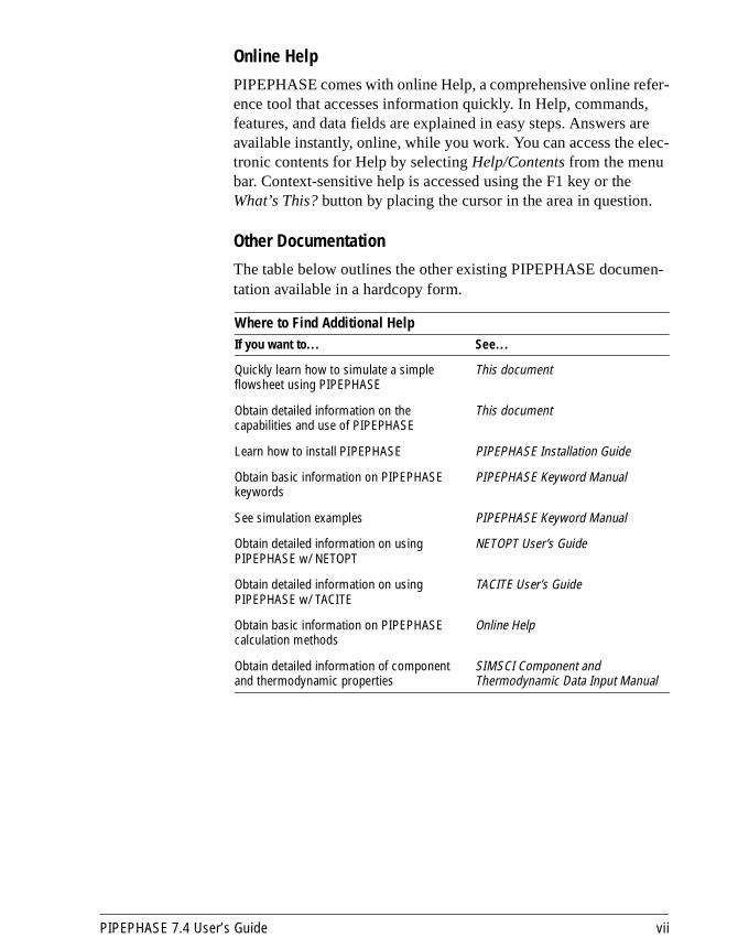
Other Documentation
The table below outlines the other existing PIPEPHASE documen-tation available in a hardcopy form.
Where to Find Additional HelpIf you want to... See...
Quickly learn how to simulate a simple flowsheet using PIPEPHASE
This document
Obtain detailed information on the capabilities and use of PIPEPHASE
This document
Learn how to install PIPEPHASE PIPEPHASE Installation Guide
Obtain basic information on PIPEPHASE keywords
PIPEPHASE Keyword Manual
See simulation examples PIPEPHASE Keyword Manual
Obtain detailed information on using PIPEPHASE w/ NETOPT
NETOPT User’s Guide
Obtain detailed information on using PIPEPHASE w/ TACITE
TACITE User’s Guide
Obtain basic information on PIPEPHASE calculation methods
Online Help
Obtain detailed information of component and thermodynamic properties
SIMSCI Component and Thermodynamic Data Input Manual
PIPEPHASE 7.4 User’s Guide vii

Technical SupportSIMSCI and its agents around the world provide technical support and service for PIPEPHASE. If you have any questions regarding the use of the program or the interpretation of output produced by the program, contact your local SIMSCI representative for advice or consultation.
When calling one of the Technical Support Centers, be prepared to describe your problem or the type of assistance required. Also, to expedite your call, complete the following steps before calling Technical Support:
■ Have the installation CD and all provided documentation avail-able.
■ Determine the type of computer you are using.
■ Determine the amount of free disk space available on the disk on which the product is installed.
■ Note the exact actions you were taking when the problem occurred, as well as the steps you took leading up to that point.
■ Note the exact error messages that appear on your screen, as well as any other symptoms.
viii

Authorized SIMSCI Technical Support Centers
Support Center Address Tel/Fax/Internet
Western USA/Canada
IPA-SIMSCI601 Valencia Ave., Suite 100Brea, CA 92823-6346
Tel: (800) SIMSCI-1+1 (714) 579-0412
Fax: +1 (714) 579-0354E-mail: [email protected]: http://www.simsci.com
Mid USA/Virgin Islands
IPA-SIMSCI2500 City West Blvd., Suite 1200Houston, TX 77042-3029
Tel: (800) SIMSCI-1+1 (713) 683-1710
Fax: +1 (713) 683-6613E-mail: [email protected]
Eastern USA/Canada
IPA-SIMSCI3 Chelsea Parkway., Suite 309Boothwyn, PA 19061
Tel: (800) SIMSCI-1+1 (610) 364-1900
Fax: +1 (610) 364-9600E-mail: [email protected]
Europe IPA-SIMSCIHigh Bank House, Exchange St.Stockport, Cheshire, SK3 OET, UK
Tel: +(44) 161-429-6744Fax: +(44) 161-480-9063E-mail: [email protected]: 666127
Germany/Austria Invensys Deutschland GmbHHerdter Lohweg 53-5540549 Dusseldorf, Germany
Tel: +(49) 211-5966-0Fax: +(49) 211-5966-167Internet: http://www.foxboro.com/csc/index.htm
Japan Invensys Systems Engineering Gotanda Chuo Bldg (2F)2-3-5 Higashi Gotanda, Shinagawa-kuTokyo 141-022, Japan
Tel: +(81) 3-5793-4851Fax: +(81) 3-5793-4857E-mail: [email protected]
South America Invensys VenezuelaAv. Francisco de MirandaTorre Delta, Piso 12AltamiraCaracas, 1060, Venezuela
Tel: +(58) 2-267-5868Fax: +(58) 2-267-0964E-mail: [email protected]
Asia/Pacific Rim Invensys Asia12 Pandan Road609260Singapore
Tel: +(65) 768-9111Fax: +(65) 268-1291E-mail: [email protected] Satisfaction Center:[email protected]
Middle East/Africa Invensys ME DubaiP.O. Box 26430Dubai Airport Free ZoneSuite #206, (East Wing)DubaiUnited Arab Emirates
Tel: +00 (971) 4-229-4902Fax: +00 (971) 4-229-4903E-mail: [email protected]
Support Center Address Tel/Fax/Internet
PIPEPHASE 7.4 User’s Guide ix


Chapter 1Getting Started
Starting PIPEPHASEIf you do not see a PIPEPHASE 7.4 icon in a SIMSCI group window or in your Program Manager window, see the troubleshooting section in the PIPEPHASE Installation Guide.
To start PIPEPHASE:
➤ Double-click on the PIPEPHASE 7.4 icon.
The main PIPEPHASE window appears.
Figure 1-1: The PIPEPHASE Main Window
PIPEPHASE 7.4 User’s Guide 1-1
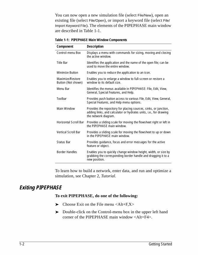
You can now open a new simulation file (select File/New), open an existing file (select File/Open), or import a keyword file (select File/
Import Keyword File). The elements of the PIPEPHASE main window are described in Table 1-1.
To learn how to build a network, enter data, and run and optimize a simulation, see Chapter 2, Tutorial.
Exiting PIPEPHASETo exit PIPEPHASE, do one of the following:
➤ Choose Exit on the File menu <Alt+F,X>
➤ Double-click on the Control-menu box in the upper left hand corner of the PIPEPHASE main window <Alt+F4>.
Table 1-1: PIPEPHASE Main Window Components
Component Description
Control-menu Box Displays a menu with commands for sizing, moving and closing the active window.
Title Bar Identifies the application and the name of the open file; can be used to move the entire window.
Minimize Button Enables you to reduce the application to an icon.
Maximize/Restore Button (Not shown)
Enables you to enlarge a window to full-screen or restore a window to its default size.
Menu Bar Identifies the menus available in PIPEPHASE: File, Edit, View, General, Special Features, and Help.
Toolbar Provides push button access to various File, Edit, View, General, Special Features, and Help menu options.
Main Window Provides the repository for placing sources, sinks, or junction, adding links, and calculator or hydrates units, i.e., for drawing the network diagram.
Horizontal Scroll Bar Provides a sliding scale for moving the flowsheet right or left in the PIPEPHASE main window.
Vertical Scroll Bar Provides a sliding scale for moving the flowsheet to up or down in the PIPEPHASE main window.
Status Bar Provides guidance, focus and error messages for the active feature or object.
Border Handles Enables you to quickly change window height, width, or size by grabbing the corresponding border handle and dragging it to a new position.
1-2 Getting Started
Manipulating the PIPEPHASE Window The PIPEPHASE window offers a variety of features that enable you to customize how PIPEPHASE appears relative to the full screen and relative to other applications.
Changing Window Size
The Windows interface provides tools for resizing each window. Some tools automatically change a window to a particular size and orientation, others enable you to control the magnification.
To display the control-menu box:
➤ Click on the control-menu box in the top left hand corner of the PIPEPHASE main window or use <Alt+Space>.
➤ Select the Move option from the menu.
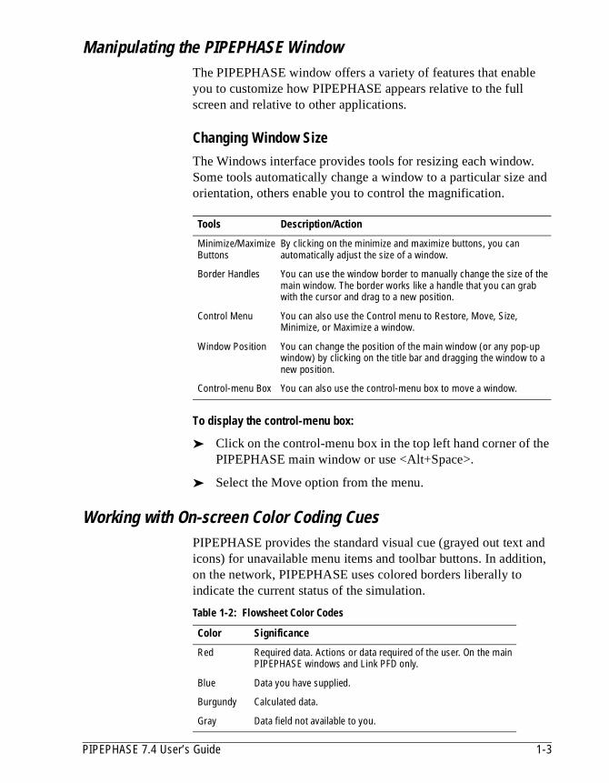
Working with On-screen Color Coding Cues PIPEPHASE provides the standard visual cue (grayed out text and icons) for unavailable menu items and toolbar buttons. In addition, on the network, PIPEPHASE uses colored borders liberally to indicate the current status of the simulation.
Tools Description/Action
Minimize/Maximize Buttons
By clicking on the minimize and maximize buttons, you can automatically adjust the size of a window.
Border Handles You can use the window border to manually change the size of the main window. The border works like a handle that you can grab with the cursor and drag to a new position.
Control Menu You can also use the Control menu to Restore, Move, Size, Minimize, or Maximize a window.
Window Position You can change the position of the main window (or any pop-up window) by clicking on the title bar and dragging the window to a new position.
Control-menu Box You can also use the control-menu box to move a window.
Table 1-2: Flowsheet Color Codes
Color Significance
Red Required data. Actions or data required of the user. On the main PIPEPHASE windows and Link PFD only.
Blue Data you have supplied.
Burgundy Calculated data.
Gray Data field not available to you.
PIPEPHASE 7.4 User’s Guide 1-3

Using the Menus The names of the PIPEPHASE main menus appear on the menu bar. From these menus, you can access most PIPEPHASE operations.
To display a menu:
➤ Click on the menu name or press <Alt+n> where n is the underlined letter in the menu name.
For example, to display the File menu, either click on File, or press <Alt+F>.
Figure 1-2: File Menu Figure 1-3: Edit Menu
Figure 1-4: View Menu Figure 1-5: General Menu
1-4 Getting Started

Choosing a Menu Item To choose a menu item, do one of the following:
➤ Click on the desired item.
➤ Use the arrow keys to highlight the item then press <Enter>.
➤ Use the accelerator keys.
Using the Toolbar ButtonsFigure 1-8: Toolbar Buttons
The toolbar contains four groups of buttons:
➤ File Manipulation Buttons
➤ Structure and Unit Operation Buttons
➤ Calculation Options, Optimization, and Property Buttons
➤ Zoom and Redraw Buttons
Figure 1-6: Special Features Menu Figure 1-7: Help Menu
Note: Grayed out icons indicate that those functions are currently in passive mode and will become active when necessary.
PIPEPHASE 7.4 User’s Guide 1-5
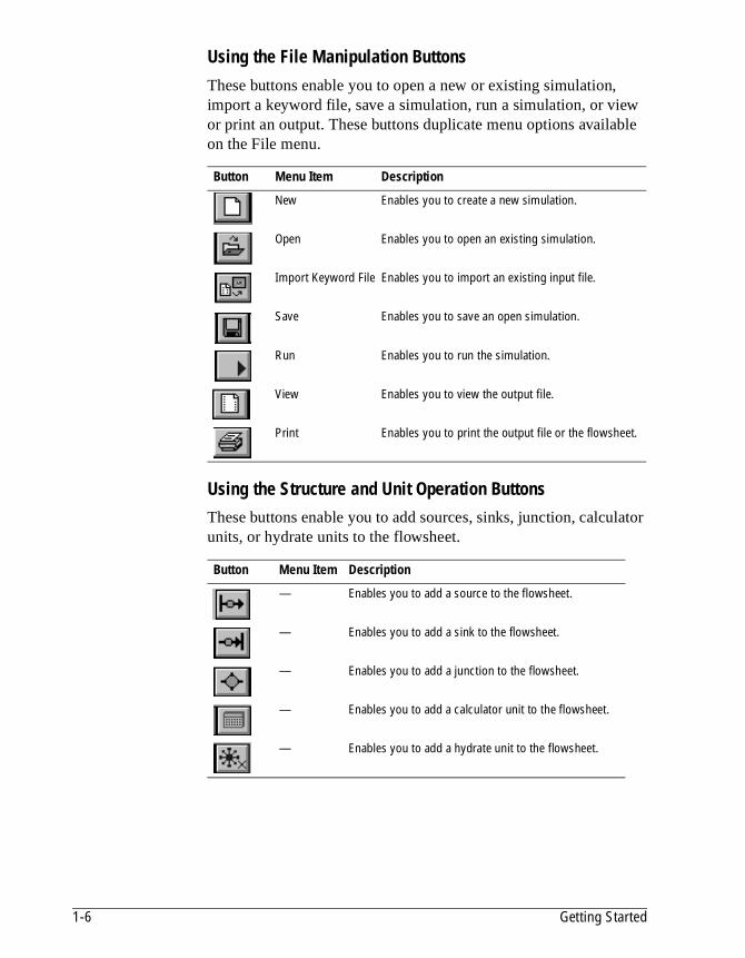
Using the File Manipulation Buttons
These buttons enable you to open a new or existing simulation, import a keyword file, save a simulation, run a simulation, or view or print an output. These buttons duplicate menu options available on the File menu.
Using the Structure and Unit Operation Buttons These buttons enable you to add sources, sinks, junction, calculator units, or hydrate units to the flowsheet.
Button Menu Item Description
New Enables you to create a new simulation.
Open Enables you to open an existing simulation.
Import Keyword File Enables you to import an existing input file.
Save Enables you to save an open simulation.
Run Enables you to run the simulation.
View Enables you to view the output file.
Print Enables you to print the output file or the flowsheet.
Button Menu Item Description
— Enables you to add a source to the flowsheet.
— Enables you to add a sink to the flowsheet.
— Enables you to add a junction to the flowsheet.
— Enables you to add a calculator unit to the flowsheet.
— Enables you to add a hydrate unit to the flowsheet.
1-6 Getting Started
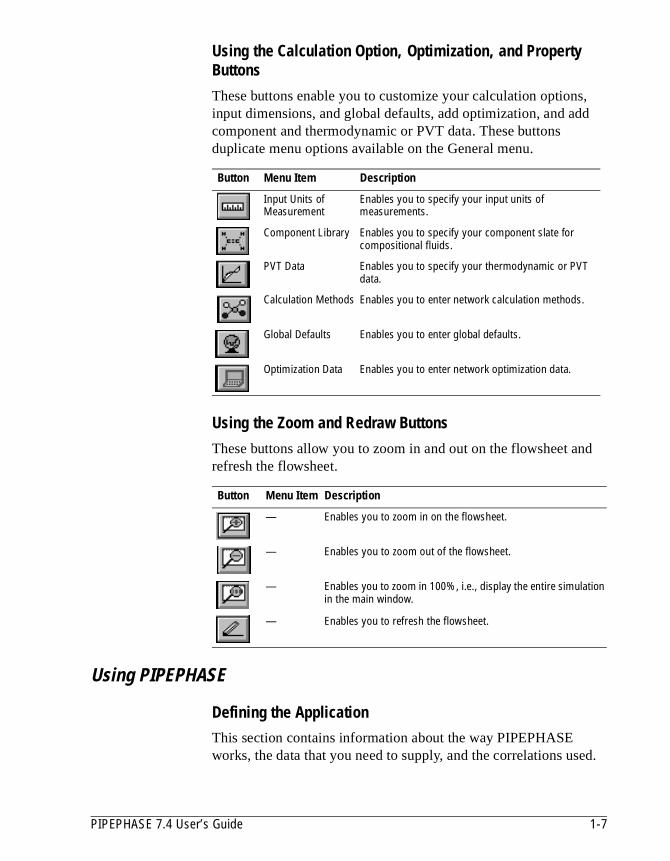
Using the Calculation Option, Optimization, and Property Buttons
These buttons enable you to customize your calculation options, input dimensions, and global defaults, add optimization, and add component and thermodynamic or PVT data. These buttons duplicate menu options available on the General menu.
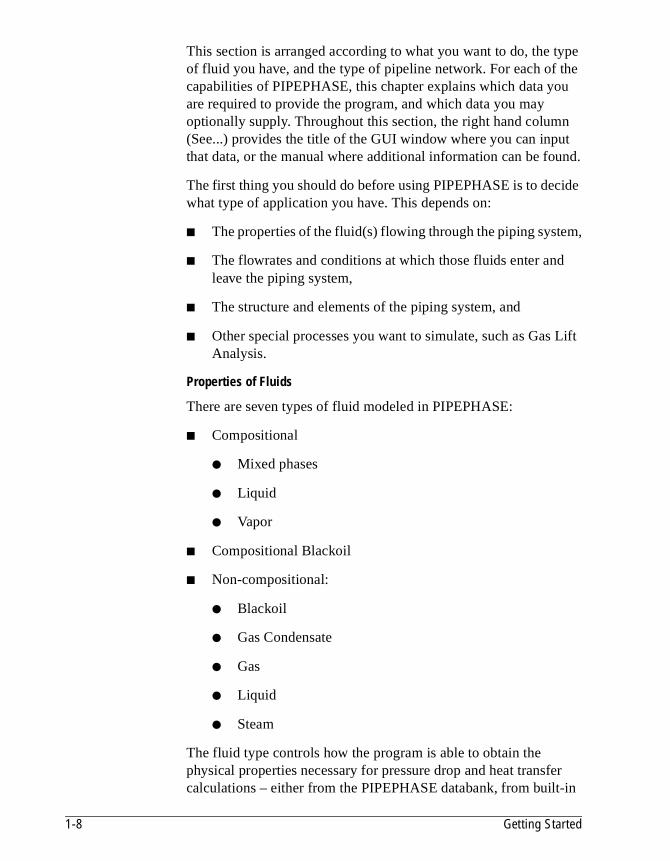
Using the Zoom and Redraw Buttons
These buttons allow you to zoom in and out on the flowsheet and refresh the flowsheet.
Using PIPEPHASE
Defining the ApplicationThis section contains information about the way PIPEPHASE works, the data that you need to supply, and the correlations used.
Button Menu Item Description
Input Units of Measurement
Enables you to specify your input units of measurements.
Component Library Enables you to specify your component slate for compositional fluids.
PVT Data Enables you to specify your thermodynamic or PVT data.
Calculation Methods Enables you to enter network calculation methods.
Global Defaults Enables you to enter global defaults.
Optimization Data Enables you to enter network optimization data.
Button Menu Item Description
— Enables you to zoom in on the flowsheet.
— Enables you to zoom out of the flowsheet.
— Enables you to zoom in 100%, i.e., display the entire simulation in the main window.
— Enables you to refresh the flowsheet.
PIPEPHASE 7.4 User’s Guide 1-7
in
This section is arranged according to what you want to do, the type of fluid you have, and the type of pipeline network. For each of the capabilities of PIPEPHASE, this chapter explains which data you are required to provide the program, and which data you may optionally supply. Throughout this section, the right hand column (See...) provides the title of the GUI window where you can input that data, or the manual where additional information can be found.
The first thing you should do before using PIPEPHASE is to decide what type of application you have. This depends on:
■ The properties of the fluid(s) flowing through the piping system,
■ The flowrates and conditions at which those fluids enter and leave the piping system,
■ The structure and elements of the piping system, and
■ Other special processes you want to simulate, such as Gas Lift Analysis.
Properties of Fluids
There are seven types of fluid modeled in PIPEPHASE:
■ Compositional
● Mixed phases
● Liquid
● Vapor
■ Compositional Blackoil
■ Non-compositional:
● Blackoil
● Gas Condensate
● Gas
● Liquid
● Steam
The fluid type controls how the program is able to obtain the physical properties necessary for pressure drop and heat transfer calculations – either from the PIPEPHASE databank, from built-
1-8 Getting Started

in f
ures to
empirical correlations, or from user-supplied input. Steam is a special case of a non-compositional fluid, for which PIPEPHASE uses the GPSA steam tables.
Compositional fluids are defined as mixtures of chemical components with a known composition. For compositional fluids, PIPEPHASE will calculate the phase separation whenever prevailing process fluid conditions are required. However, you may instruct PIPEPHASE to assume the fluid is one phase at all times, thus reducing the time the program takes to solve by continually bypassing the vapor-liquid equilibrium (flash) calculation.
Non-compositional gases and liquids are single-phase. Blackoil is a liquid-dominated, two-phase model. Gas Condensate is a gas-dominated, two-phase model. Steam is a single component, two-phase model.
Optimization
PIPEPHASE can optimize network problems of virtually any size. You can minimize or maximize any objective function or even tune your simulation to match measured data, while satisfying operational or design constraints. A PIPEPHASE model can be optimized over time resulting in efficient optimized design, planning, forecasting, and operation of a field.
Link to Reservoir Simulator Models
PIPEPHASE’s Reservoir Interface allows you to link the network simulator to link to Reservoir Simulation models such as the Eclipse reservoir simulation model. This integrated solution provides greater simulation consistency and accuracy, resulting savings of millions of dollars over the lifetime of a field in terms oplanning and scheduling.
Flows and Conditions of Fluids
Fluids enter piping systems at sources and leave at sinks. Fluids with different properties may enter at different sources, but they must all be of the same type.
In general, you have to assign flowrates, temperatures and pressto sources and/or sinks. For compositional fluids, you also haveassign compositions to the source fluids. The exceptions are explained below in What PIPEPHASE Calculates.
PIPEPHASE 7.4 User’s Guide 1-9

Gaslift and Sphering
Two special applications, relevant to oil production and gas transportation, can be modeled with PIPEPHASE. You can use PIPEPHASE to investigate the effects of lift gas on well production and optimize the allocation of limited lift gas for multiple wells. Sphering or Pigging is used to increase gas flow efficiency in wet gas and gas dominated multiphase pipelines.
Piping Structure
Before beginning to input problem data to PIPEPHASE, it is important that you convert the structure of the piping system into a simpler schematic representation of the relevant nodes (i.e., sources, junctions, and sinks) and links. You must label each node and link both uniquely and logically for future reference.
What PIPEPHASE Calculates
PIPEPHASE solves the equations that define the relationship between pressure drop and flowrate. PIPEPHASE can also calculate heat losses and gains.
With a single link, PIPEPHASE will calculate the pressure drop for a known flowrate. Alternatively, for a given pressure drop, PIPEPHASE will calculate the flowrate.
With a network configuration, you may supply a combination of known flowrates and pressures at sources and/or sinks and PIPEPHASE will calculate the unknowns. The combination of knowns that you are allowed to supply are explained later on.
Rating, Design, Case Studies, and Nodal Analysis
PIPEPHASE works in both rating and design modes. In rating mode, you supply data about the pipes, fittings and equipment and PIPEPHASE calculates the pressure and temperature profiles. In design mode, PIPEPHASE calculates line sizes. Case Studies can be performed in either mode. Nodal Analyses can be performed on single links.
Global Settings
Before you provide PIPEPHASE with information about the fluid and piping structure of your problem, global parameters may be set and the problem definition described. Choices can be made on
1-10 Getting Started
ts nits t s
control of the simulation, define the input units, specify how much output you want, and set global defaults for use throughout the simulation.
Units of Measurement
PIPEPHASE allows you to construct a group of units of measure (or “dimensions”) which are to be used throughout the entire simulation input. However, you can locally override individual uniof measure where necessary. The output will always be in the usupplied on the Input Dimensions window, unless specific outpuoverrides or supplements are provided on the Output Dimensionwindow.
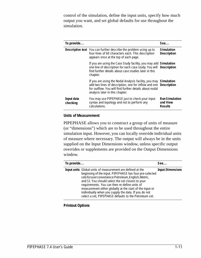
Printout Options
To provide... See...
Descriptive text You can further describe the problem using up to four lines of 60 characters each. This description appears once at the top of each page.
Simulation Description
If you are using the Case Study facility, you may add one line of description for each case study. You will find further details about case studies later in this chapter.
Simulation Description
If you are using the Nodal Analysis facility, you may add two lines of description, one for inflow and one for outflow. You will find further details about nodal analysis later in this chapter.
Simulation Description
Input data checking
You may use PIPEPHASE just to check your input syntax and topology and not to perform any calculations.
Run Simulation and View Results
To provide... See...
Input units Global units of measurement are defined at the beginning of the input. PIPEPHASE has four pre-selected sets for user convenience: Petroleum, English, Metric, and SI. You should select the set closest to your requirements. You can then re-define units of measurement either globally at the start of the input or individually when you supply the data. If you do not select a set, PIPEPHASE defaults to the Petroleum set.
Input Dimensions
PIPEPHASE 7.4 User’s Guide 1-11
ill ple
are
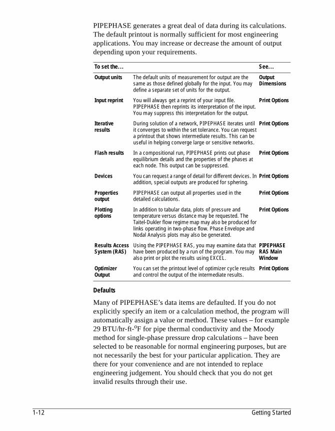
PIPEPHASE generates a great deal of data during its calculations. The default printout is normally sufficient for most engineering applications. You may increase or decrease the amount of output depending upon your requirements.
Defaults
Many of PIPEPHASE’s data items are defaulted. If you do not explicitly specify an item or a calculation method, the program wautomatically assign a value or method. These values – for exam29 BTU/hr-ft-oF for pipe thermal conductivity and the Moody method for single-phase pressure drop calculations – have beenselected to be reasonable for normal engineering purposes, butnot necessarily the best for your particular application. They arethere for your convenience and are not intended to replace engineering judgement. You should check that you do not get invalid results through their use.
To set the... See...
Output units The default units of measurement for output are the same as those defined globally for the input. You may define a separate set of units for the output.
Output Dimensions
Input reprint You will always get a reprint of your input file. PIPEPHASE then reprints its interpretation of the input. You may suppress this interpretation for the output.
Print Options
Iterative results
During solution of a network, PIPEPHASE iterates until it converges to within the set tolerance. You can request a printout that shows intermediate results. This can be useful in helping converge large or sensitive networks.
Print Options
Flash results In a compositional run, PIPEPHASE prints out phase equilibrium details and the properties of the phases at each node. This output can be suppressed.
Print Options
Devices You can request a range of detail for different devices. In addition, special outputs are produced for sphering.
Print Options
Properties output
PIPEPHASE can output all properties used in the detailed calculations.
Print Options
Plotting options
In addition to tabular data, plots of pressure and temperature versus distance may be requested. The Taitel-Dukler flow regime map may also be produced for links operating in two-phase flow. Phase Envelope and Nodal Analysis plots may also be generated.
Print Options
Results Access System (RAS)
Using the PIPEPHASE RAS, you may examine data that have been produced by a run of the program. You may also print or plot the results using EXCEL.
PIPEPHASE RAS Main Window
Optimizer Output
You can set the printout level of optimizer cycle results and control the output of the intermediate results.
Print Options
1-12 Getting Started

e ss
e
For convenience, PIPEPHASE allows you to change some defaults globally at the start of the input.
Defining Fluid Properties
PIPEPHASE requires the properties of the fluid to calculate pressure drops and heat transfer, and phase ratios. There are two major classifications of fluid models: compositional and non-compositional.
A fluid model is compositional when it can be defined in terms of its individual components either directly or via an assay curve. PIPEPHASE will then predict the fluid’s properties by applying thappropriate mixing rules to the pure component properties. UnlePIPEPHASE is instructed otherwise, it will perform phase equilibrium calculations for the fluid and determine the quantity and properties of the liquid and vapor phases.
A fluid model is non-compositional when it is defined with averagcorrelated properties.
To define... See...
Flow device parameters
You can specify global values for the pipe, riser, tubing and annulus inside diameter, the surrounding medium, and the parameters associated with pressure drop and heat transfer. You can override these settings for individual pipes.
Global Defaults
Heat Transfer You can define the heat transfer from pipes, risers, tubings, and annuli as an overall coefficient or by defining the parameters - viscosity, conductivity, velocity, etc. - for the surrounding soil, air, or water. You can select a medium and optionally override these settings for individual pipes. You can globally suppress heat transfer calculations and then reinstate them for individual pipes, risers, tubings, and annuli.
Global Defaults
Pressure drop methods
You can globally set the pressure drop method and the Palmer parameters for liquid holdup. You can override the pressure drop method for individual pipes, risers, tubings, and annuli.
Global Defaults
Transitional flow
You can globally set the transitional Reynolds Number between laminar and turbulent flow regimes.
Global Defaults
Limits You can change the maximum and minimum values of temperature and pressure for flash calculations. If the program detects conditions outside these limits, warning messages will be presented in the output.
Global Defaults
PIPEPHASE 7.4 User’s Guide 1-13
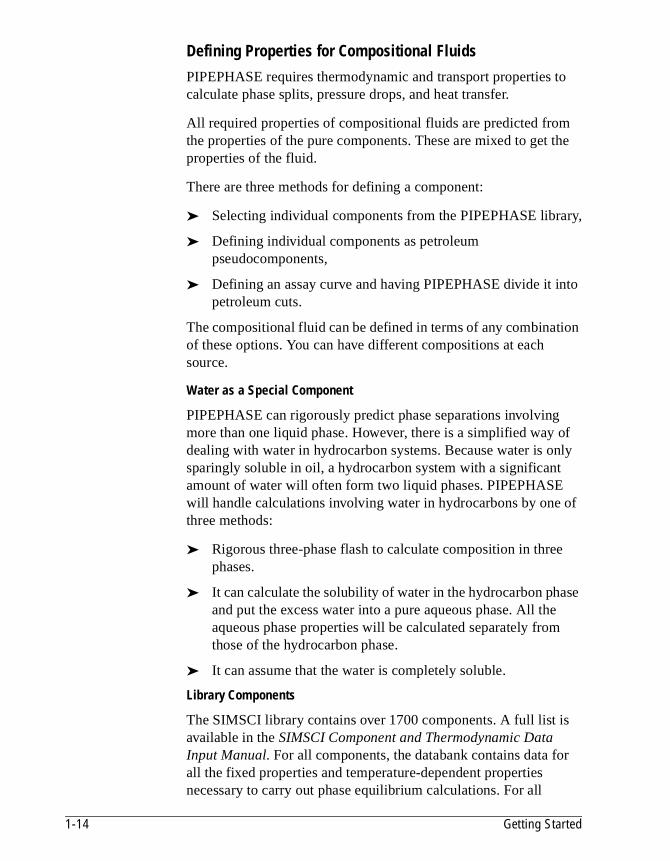
Defining Properties for Compositional Fluids
PIPEPHASE requires thermodynamic and transport properties to calculate phase splits, pressure drops, and heat transfer.
All required properties of compositional fluids are predicted from the properties of the pure components. These are mixed to get the properties of the fluid.
There are three methods for defining a component:
➤ Selecting individual components from the PIPEPHASE library,
➤ Defining individual components as petroleum pseudocomponents,
➤ Defining an assay curve and having PIPEPHASE divide it into petroleum cuts.
The compositional fluid can be defined in terms of any combination of these options. You can have different compositions at each source.
Water as a Special Component
PIPEPHASE can rigorously predict phase separations involving more than one liquid phase. However, there is a simplified way of dealing with water in hydrocarbon systems. Because water is only sparingly soluble in oil, a hydrocarbon system with a significant amount of water will often form two liquid phases. PIPEPHASE will handle calculations involving water in hydrocarbons by one of three methods:
➤ Rigorous three-phase flash to calculate composition in three phases.
➤ It can calculate the solubility of water in the hydrocarbon phase and put the excess water into a pure aqueous phase. All the aqueous phase properties will be calculated separately from those of the hydrocarbon phase.
➤ It can assume that the water is completely soluble.
Library Components
The SIMSCI library contains over 1700 components. A full list is available in the SIMSCI Component and Thermodynamic Data Input Manual. For all components, the databank contains data for all the fixed properties and temperature-dependent properties necessary to carry out phase equilibrium calculations. For all
1-14 Getting Started
east
s nd nt.
common components, the databank also contains a full set of transport properties necessary to carry out pressure drop and heat transfer calculations. If you need to supplement the data, or override the library data with your own, you may do so.
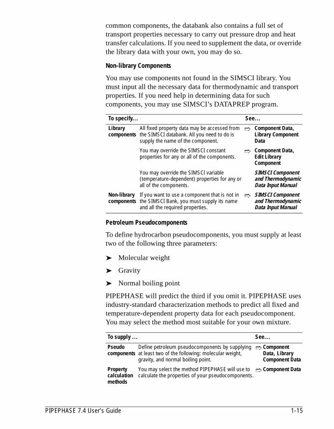
Non-library Components
You may use components not found in the SIMSCI library. You must input all the necessary data for thermodynamic and transport properties. If you need help in determining data for such components, you may use SIMSCI’s DATAPREP program.
Petroleum Pseudocomponents
To define hydrocarbon pseudocomponents, you must supply at ltwo of the following three parameters:
➤ Molecular weight
➤ Gravity
➤ Normal boiling point
PIPEPHASE will predict the third if you omit it. PIPEPHASE useindustry-standard characterization methods to predict all fixed atemperature-dependent property data for each pseudocomponeYou may select the method most suitable for your own mixture.
To specify... See...
Library components
All fixed property data may be accessed from the SIMSCI databank. All you need to do is supply the name of the component.
➱ Component Data, Library Component Data
You may override the SIMSCI constant properties for any or all of the components.
➱ Component Data, Edit Library Component
You may override the SIMSCI variable (temperature-dependent) properties for any or all of the components.
SIMSCI Component and Thermodynamic Data Input Manual
Non-library components
If you want to use a component that is not in the SIMSCI Bank, you must supply its name and all the required properties.
➱ SIMSCI Component and Thermodynamic Data Input Manual
To supply ... See...
Pseudocomponents
Define petroleum pseudocomponents by supplying at least two of the following: molecular weight, gravity, and normal boiling point.
➱ Component Data, Library Component Data
Property calculation methods
You may select the method PIPEPHASE will use to calculate the properties of your pseudocomponents.
➱ Component Data
PIPEPHASE 7.4 User’s Guide 1-15
rty E.
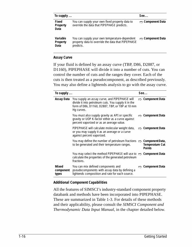
Assay Curve
If your fluid is defined by an assay curve (TBP, D86, D2887, or D1160), PIPEPHASE will divide it into a number of cuts. You can control the number of cuts and the ranges they cover. Each of the cuts is then treated as a pseudocomponent, as described previously. You may also define a lightends analysis to go with the assay curve.
Additional Component Capabilities
All the features of SIMSCI’s industry-standard component propedatabank and methods have been incorporated into PIPEPHASThese are summarized in Table 1-3. For details of these methods and their applicability, please consult the SIMSCI Component and Thermodynamic Data Input Manual, in the chapter detailed below.
Fixed Property Data
You can supply your own fixed property data to override the data that PIPEPHASE predicts.
➱ Component Data
Variable Property Data
You can supply your own temperature-dependent property data to override the data that PIPEPHASE predicts.
➱ Component Data
To supply ... See...
Assay Data You supply an assay curve, and PIPEPHASE will divide it into petroleum cuts. You supply it in the form of D86, D1160, D2887, TBP, or TBP at 10 mm Hg curves.
➱ Component Data
You must also supply gravity as API or specific gravity or UOP K-factor either as a curve against percent vaporized or as an average value.
➱ Component Data
PIPEPHASE will calculate molecular weight data, or you may supply it as an average or a curve against percent vaporized.
➱ Component Data
You may define the number of petroleum fractions to be generated and their temperature ranges.
➱ Component Data, Temperature Cut Points
You may select the method PIPEPHASE will use to calculate the properties of the generated petroleum fractions.
➱ Component Data
Mixed component types
You can mix defined components and pseudocomponents with assay data by defining a lightends composition and rate for each source.
➱ Component Data
To supply ... See...
1-16 Getting Started
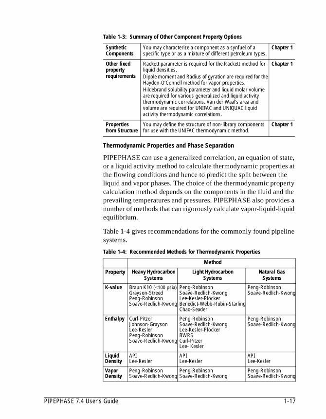
Thermodynamic Properties and Phase Separation
PIPEPHASE can use a generalized correlation, an equation of state, or a liquid activity method to calculate thermodynamic properties at the flowing conditions and hence to predict the split between the liquid and vapor phases. The choice of the thermodynamic property calculation method depends on the components in the fluid and the prevailing temperatures and pressures. PIPEPHASE also provides a number of methods that can rigorously calculate vapor-liquid-liquid equilibrium.
Table 1-4 gives recommendations for the commonly found pipeline systems.
Table 1-3: Summary of Other Component Property Options
Synthetic Components
You may characterize a component as a synfuel of a specific type or as a mixture of different petroleum types.
Chapter 1
Other fixed property requirements
Rackett parameter is required for the Rackett method for liquid densities.Dipole moment and Radius of gyration are required for the Hayden-O’Connell method for vapor properties.Hildebrand solubility parameter and liquid molar volume are required for various generalized and liquid activity thermodynamic correlations. Van der Waal’s area and volume are required for UNIFAC and UNIQUAC liquid activity thermodynamic correlations.
Chapter 1
Properties from Structure
You may define the structure of non-library components for use with the UNIFAC thermodynamic method.
Chapter 1
Table 1-4: Recommended Methods for Thermodynamic Properties
Method
Property Heavy Hydrocarbon Systems
Light HydrocarbonSystems
Natural GasSystems
K-value Braun K10 (<100 psia)Grayson-StreedPeng-RobinsonSoave-Redlich-Kwong
Peng-RobinsonSoave-Redlich-KwongLee-Kesler-PlöckerBenedict-Webb-Rubin-Starling Chao-Seader
Peng-RobinsonSoave-Redlich-Kwong
Enthalpy Curl-PitzerJohnson-GraysonLee-KeslerPeng-RobinsonSoave-Redlich-Kwong
Peng-RobinsonSoave-Redlich-KwongLee-Kesler-PlöckerBWRSCurl-PitzerLee- Kesler
Peng-RobinsonSoave-Redlich-Kwong
Liquid Density
APILee-Kesler
APILee-Kesler
APILee-Kesler
Vapor Density
Peng-RobinsonSoave-Redlich-Kwong
Peng-RobinsonSoave-Redlich-Kwong
Peng-RobinsonSoave-Redlich-Kwong
PIPEPHASE 7.4 User’s Guide 1-17
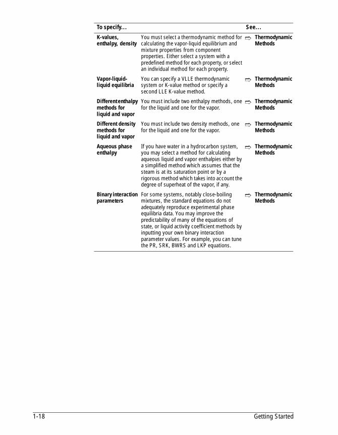
To specify... See...
K-values, enthalpy, density
You must select a thermodynamic method for calculating the vapor-liquid equilibrium and mixture properties from component properties. Either select a system with a predefined method for each property, or select an individual method for each property.
➱ Thermodynamic Methods
Vapor-liquid-liquid equilibria
You can specify a VLLE thermodynamic system or K-value method or specify a second LLE K-value method.
➱ Thermodynamic Methods
Different enthalpy methods for liquid and vapor
You must include two enthalpy methods, one for the liquid and one for the vapor.
➱ Thermodynamic Methods
Different density methods for liquid and vapor
You must include two density methods, one for the liquid and one for the vapor.
➱ Thermodynamic Methods
Aqueous phase enthalpy
If you have water in a hydrocarbon system, you may select a method for calculating aqueous liquid and vapor enthalpies either by a simplified method which assumes that the steam is at its saturation point or by a rigorous method which takes into account the degree of superheat of the vapor, if any.
➱ Thermodynamic Methods
Binary interaction parameters
For some systems, notably close-boiling mixtures, the standard equations do not adequately reproduce experimental phase equilibria data. You may improve the predictability of many of the equations of state, or liquid activity coefficient methods by inputting your own binary interaction parameter values. For example, you can tune the PR, SRK, BWRS and LKP equations.
➱ Thermodynamic Methods
1-18 Getting Started
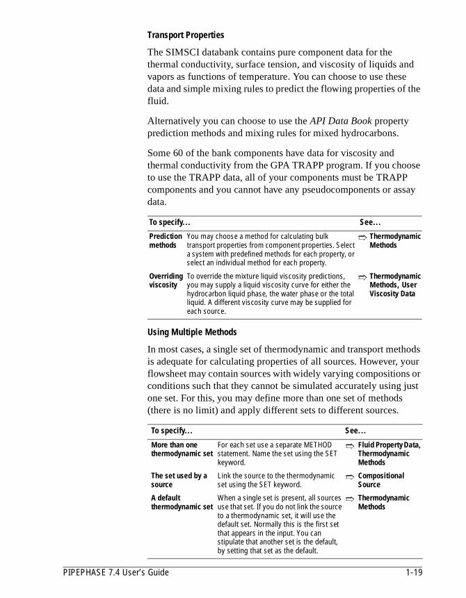
Transport Properties
The SIMSCI databank contains pure component data for the thermal conductivity, surface tension, and viscosity of liquids and vapors as functions of temperature. You can choose to use these data and simple mixing rules to predict the flowing properties of the fluid.
Alternatively you can choose to use the API Data Book property prediction methods and mixing rules for mixed hydrocarbons.
Some 60 of the bank components have data for viscosity and thermal conductivity from the GPA TRAPP program. If you choose to use the TRAPP data, all of your components must be TRAPP components and you cannot have any pseudocomponents or assay data.
Using Multiple Methods
In most cases, a single set of thermodynamic and transport methods is adequate for calculating properties of all sources. However, your flowsheet may contain sources with widely varying compositions or conditions such that they cannot be simulated accurately using just one set. For this, you may define more than one set of methods (there is no limit) and apply different sets to different sources.
To specify... See...
Prediction methods
You may choose a method for calculating bulk transport properties from component properties. Select a system with predefined methods for each property, or select an individual method for each property.
➱ Thermodynamic Methods
Overriding viscosity
To override the mixture liquid viscosity predictions, you may supply a liquid viscosity curve for either the hydrocarbon liquid phase, the water phase or the total liquid. A different viscosity curve may be supplied for each source.
➱ Thermodynamic Methods, User Viscosity Data
To specify... See...
More than one thermodynamic set
For each set use a separate METHOD statement. Name the set using the SET keyword.
➱ Fluid Property Data, Thermodynamic Methods
The set used by a source
Link the source to the thermodynamic set using the SET keyword.
➱ Compositional Source
A default thermodynamic set
When a single set is present, all sources use that set. If you do not link the source to a thermodynamic set, it will use the default set. Normally this is the first set that appears in the input. You can stipulate that another set is the default, by setting that set as the default.
➱ Thermodynamic Methods
PIPEPHASE 7.4 User’s Guide 1-19

s are ls
Additional Thermodynamic Capabilities
All of SIMSCI’s industry-standard thermophysical property calculation methods have been incorporated into PIPEPHASE. These are summarized in Table 1-5. For details of these methods and their applicability, please consult Chapter 2 in the SIMSCI Component and Thermodynamic Data Input Manual.
Defining Properties for Non-compositional FluidsA non-compositional fluid model must be defined as blackoil, gacondensate, liquid, gas, or steam. Blackoil and gas condensate two-phase, with one phase dominant. Gas and liquid fluid modeare single-phase. Steam may be single- or two-phase.
Table 1-5: Summary of Other Thermodynamic Options
Generalized Correlations
Grayson-StreedImproved-Grayson-StreedGrayson-Streed-ErbarBraun-K10
Chao-SeaderChao-Seader-ErbarIdeal
Equations of State
Soave-Redlich-KwongSRK-Kabadi-DannerSRK-Huron-VidalSRK-Panagiotopoulos-ReidSRK-ModifiedSRK-SIMSCISRK-Hexamer
Panagiotopoulos-ReidPeng-RobinsonPR-Huron-VidalPR-Panagiotopoulos-ReidBWRSUniwaals
Liquid Activity Methods
Non-random Two-liquid EquationUniversal Quasi-chemical (UNIQUAC)van LaarWilsonMargulesRegular Solution TheoryFlory-Huggins Theory
Universal Functional Activity Coefficient (UNIFAC)Lyngby-modified UNIFACDortmund-modified UNIFACModified UNIFAC methodFree volume modification to UNIFACIdeal
Special Packages
GlycolSourGPA Sour Water
AmineAlcohol
Other Features
Heat of MixingPoynting Correction
Henry’s LawAmine Residence TimeCorrection
To... See...
Define the fluid You must tell PIPEPHASE the type of fluid you have; blackoil, gas condensate, liquid, gas, or steam.
➱ Simulation Definition
Supply different data for different sources
You may supply specific gravities for each source.
➱ Source
1-20 Getting Started
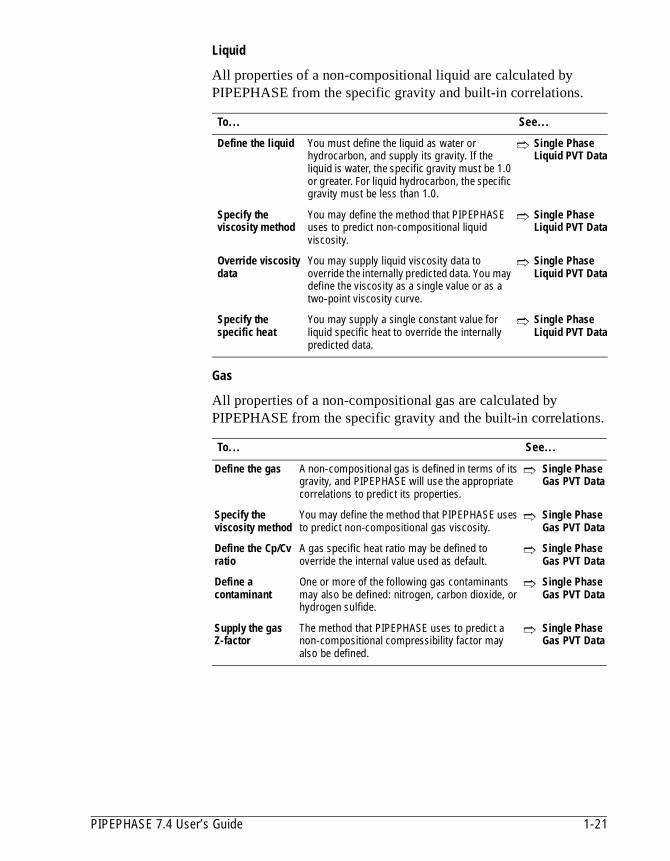
Liquid
All properties of a non-compositional liquid are calculated by PIPEPHASE from the specific gravity and built-in correlations.
Gas
All properties of a non-compositional gas are calculated by PIPEPHASE from the specific gravity and the built-in correlations.
To... See...
Define the liquid You must define the liquid as water or hydrocarbon, and supply its gravity. If the liquid is water, the specific gravity must be 1.0 or greater. For liquid hydrocarbon, the specific gravity must be less than 1.0.
➱ Single Phase Liquid PVT Data
Specify the viscosity method
You may define the method that PIPEPHASE uses to predict non-compositional liquid viscosity.
➱ Single Phase Liquid PVT Data
Override viscosity data
You may supply liquid viscosity data to override the internally predicted data. You may define the viscosity as a single value or as a two-point viscosity curve.
➱ Single Phase Liquid PVT Data
Specify the specific heat
You may supply a single constant value for liquid specific heat to override the internally predicted data.
➱ Single Phase Liquid PVT Data
To... See...
Define the gas A non-compositional gas is defined in terms of its gravity, and PIPEPHASE will use the appropriate correlations to predict its properties.
➱ Single Phase Gas PVT Data
Specify the viscosity method
You may define the method that PIPEPHASE uses to predict non-compositional gas viscosity.
➱ Single Phase Gas PVT Data
Define the Cp/Cv ratio
A gas specific heat ratio may be defined to override the internal value used as default.
➱ Single Phase Gas PVT Data
Define a contaminant
One or more of the following gas contaminants may also be defined: nitrogen, carbon dioxide, or hydrogen sulfide.
➱ Single Phase Gas PVT Data
Supply the gasZ-factor
The method that PIPEPHASE uses to predict a non-compositional compressibility factor may also be defined.
➱ Single Phase Gas PVT Data
PIPEPHASE 7.4 User’s Guide 1-21
s y
s.
m
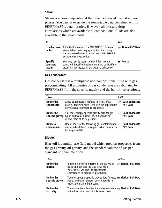
Steam
Steam is a non-compositional fluid that is allowed to exist in two phases. You cannot override the steam table data contained within PIPEPHASE’s data libraries. However, all pressure drop correlations which are available to compositional fluids are also available to the steam model.
Gas Condensate
Gas condensate is a multiphase non-compositional fluid with gapredominating. All properties of gas condensate are calculated bPIPEPHASE from the specific gravity and the built-in correlation
Blackoil
Blackoil is a multiphase fluid model which predicts properties frothe gas gravity, oil gravity, and the standard volume of gas per standard unit volume of oil.
To... See...
Use the steam tables
If the fluid is steam, use PIPEPHASE ‘s internal steam tables. You may specify that the gravity of the condensed water is more than 1.0 to take into account dissolved solids.
➱ Stream PVT Data
Specify saturated steam
You may specify steam quality if the steam is saturated. Specify the temperature and quality if the steam is superheated or the water is subcooled.
➱ Source
To... See...
Define the condensate
A gas condensate is defined in terms of its gravity, and PIPEPHASE will use the appropriate correlations to predict its properties.
➱ Gas Condensate PVT Data
Define the specific gravity
You must supply specific gravity data for gas, liquid and water phases, even if you do not expect them all to be present.
➱ Gas Condensate PVT Data
Define a contaminant
One or more of the following gas contaminants may also be defined: nitrogen, carbon dioxide, or hydrogen sulfide.
➱ Gas Condensate PVT Data
To... See...
Define the Blackoil
Blackoil is defined in terms of the gravity of its oil and gas and the Gas to Oil ratio. PIPEPHASE will use the appropriate correlations to predict its properties.
➱Blackoil PVT Data
Define the specific gravity
You must supply specific gravity data for gas, liquid, and water phases, even if you do not expect them all to be present.
➱Blackoil PVT Data
Define the viscosity
You may optionally enter liquid viscosity data in the form of a two-point Antoine curve.
➱Blackoil PVT Data
1-22 Getting Started
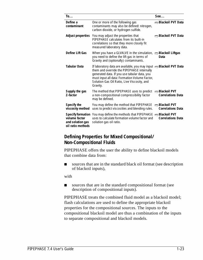
Defining Properties for Mixed Compositional/Non-Compositional FluidsPIPEPHASE offers the user the ability to define blackoil models that combine data from:
■ sources that are in the standard black oil format (see description of blackoil inputs),
with
■ sources that are in the standard compositional format (see description of compositional inputs).
PIPEPHASE treats the combined fluid model as a blackoil model; flash calculations are used to define the appropriate blackoil properties for the compositional sources. The inputs to the compositional blackoil model are thus a combination of the inputs to separate compositional and blackoil models.
Define a contaminant
One or more of the following gas contaminants may also be defined: nitrogen, carbon dioxide, or hydrogen sulfide.
➱Blackoil PVT Data
Adjust properties You may adjust the properties that PIPEPHASE calculates from its built-in correlations so that they more closely fit measured laboratory data.
➱Blackoil PVT Data
Define Lift Gas When you have a GLVALVE in the simulation, you need to define the lift gas in terms of Gravity and (optionally) contaminants.
➱Blackoil Liftgas Data
Tabular Data If laboratory data are available, you may input them and override the PIPEPHASE internally generated data. If you use tabular data, you must input all data: Formation Volume Factor, Solution Gas Oil Ratio, Live Viscosity, and Gravity.
➱Blackoil PVT Data
Supply the gas Z-factor
The method that PIPEPHASE uses to predict a non-compositional compressibility factor may be defined.
➱Blackoil PVT Correlations Data
Specify the viscosity method
You may define the method that PIPEPHASE uses to predict viscosities and blending rules.
➱Blackoil PVT Correlations Data
Specify formation volume factor and solution gas oil ratio methods
You may define the methods that PIPEPHASE uses to calculate formation volume factor and solution gas oil ratio.
➱Blackoil PVT Correlations Data
To... See...
PIPEPHASE 7.4 User’s Guide 1-23
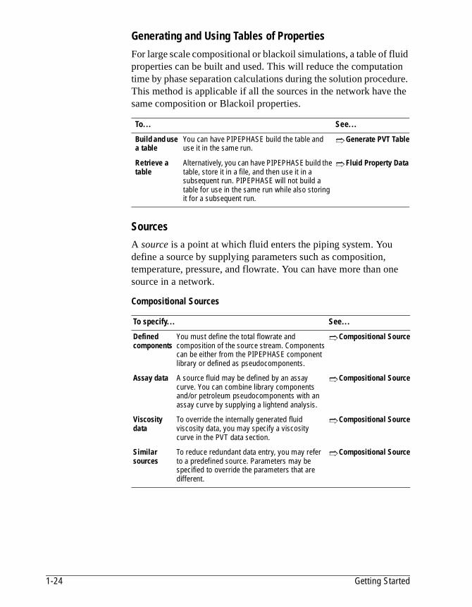
Generating and Using Tables of Properties
For large scale compositional or blackoil simulations, a table of fluid properties can be built and used. This will reduce the computation time by phase separation calculations during the solution procedure. This method is applicable if all the sources in the network have the same composition or Blackoil properties.
SourcesA source is a point at which fluid enters the piping system. You define a source by supplying parameters such as composition, temperature, pressure, and flowrate. You can have more than one source in a network.
Compositional Sources
To... See...
Build and use a table
You can have PIPEPHASE build the table and use it in the same run.
➱ Generate PVT Table
Retrieve a table
Alternatively, you can have PIPEPHASE build the table, store it in a file, and then use it in a subsequent run. PIPEPHASE will not build a table for use in the same run while also storing it for a subsequent run.
➱ Fluid Property Data
To specify... See...
Defined components
You must define the total flowrate and composition of the source stream. Components can be either from the PIPEPHASE component library or defined as pseudocomponents.
➱ Compositional Source
Assay data A source fluid may be defined by an assay curve. You can combine library components and/or petroleum pseudocomponents with an assay curve by supplying a lightend analysis.
➱ Compositional Source
Viscosity data
To override the internally generated fluid viscosity data, you may specify a viscosity curve in the PVT data section.
➱ Compositional Source
Similar sources
To reduce redundant data entry, you may refer to a predefined source. Parameters may be specified to override the parameters that are different.
➱ Compositional Source
1-24 Getting Started
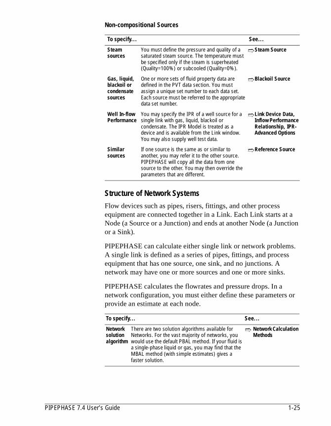
Non-compositional Sources
Structure of Network SystemsFlow devices such as pipes, risers, fittings, and other process equipment are connected together in a Link. Each Link starts at a Node (a Source or a Junction) and ends at another Node (a Junction or a Sink).
PIPEPHASE can calculate either single link or network problems. A single link is defined as a series of pipes, fittings, and process equipment that has one source, one sink, and no junctions. A network may have one or more sources and one or more sinks.
PIPEPHASE calculates the flowrates and pressure drops. In a network configuration, you must either define these parameters or provide an estimate at each node.
To specify... See...
Steam sources
You must define the pressure and quality of a saturated steam source. The temperature must be specified only if the steam is superheated (Quality=100%) or subcooled (Quality=0%).
➱Steam Source
Gas, liquid, blackoil or condensate sources
One or more sets of fluid property data are defined in the PVT data section. You must assign a unique set number to each data set. Each source must be referred to the appropriate data set number.
➱Blackoil Source
Well In-flow Performance
You may specify the IPR of a well source for a single link with gas, liquid, blackoil or condensate. The IPR Model is treated as a device and is available from the Link window. You may also supply well test data.
➱Link Device Data, Inflow Performance Relationship, IPR-Advanced Options
Similar sources
If one source is the same as or similar to another, you may refer it to the other source. PIPEPHASE will copy all the data from one source to the other. You may then override the parameters that are different.
➱Reference Source
To specify... See...
Network solution algorithm
There are two solution algorithms available for Networks. For the vast majority of networks, you would use the default PBAL method. If your fluid is a single-phase liquid or gas, you may find that the MBAL method (with simple estimates) gives a faster solution.
➱ Network Calculation Methods
PIPEPHASE 7.4 User’s Guide 1-25
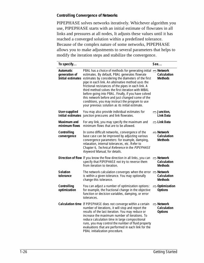
Controlling Convergence of Networks
PIPEPHASE solves networks iteratively. Whichever algorithm you use, PIPEPHASE starts with an initial estimate of flowrates in all links and pressures at all nodes, It adjusts these values until it has reached a converged solution within a predefined tolerance. Because of the complex nature of some networks, PIPEPHASE allows you to make adjustments to several parameters that helps to modify the iteration steps and stabilize the convergence.
To specify... See...
Automatic generation of Initial estimates
PBAL has a choice of methods for generating initial estimates. By default, PBAL generates flowrate estimates by considering the diameters of the first pipe in each link. An alternative method uses the frictional resistances of the pipes in each link. A third method solves the first iteration with MBAL before going into PBAL. Finally, if you have solved this network before and just changed some of the conditions, you may instruct the program to use your previous solution as its initial estimate.
➱ Network Calculation Methods
User-supplied initial estimates
You may also provide individual estimates for junction pressures and link flowrates.
➱ Junction,Link Data
Maximum and minimum flows
For any link, you may specify the maximum and minimum flows that are to be allowed.
➱ Link Data
Controlling convergence
In some difficult networks, convergence of the base case can be improved by adjusting various convergence parameters: for example, damping, relaxation, internal tolerances, etc. Refer to Chapter 6, Technical Reference in the PIPEPHASE Keyword Manual, for details.
➱ Network Calculation Methods
Direction of flow If you know the flow direction in all links, you can specify that PIPEPHASE not try to reverse them from iteration to iteration.
➱ Network Calculation Methods
Solution tolerance
The network calculation converges when the error is within a given tolerance. You may optionally change this tolerance.
➱ Network Calculation Methods
Controlling optimization
You can adjust a number of optimization options: for example, the fractional change in the objective function or decision variables, damping, or error tolerances.
➱ Optimization Options
Calculation time If PIPEPHASE does not converge within a certain number of iterations, it will stop and report the results of the last iteration. You may reduce or increase the maximum number of iterations. To reduce calculation time in large compositional runs, you may control the number of fluid property evaluations that are performed in each link for the PBAL initialization procedure.
➱ Network Calculation Options
1-26 Getting Started
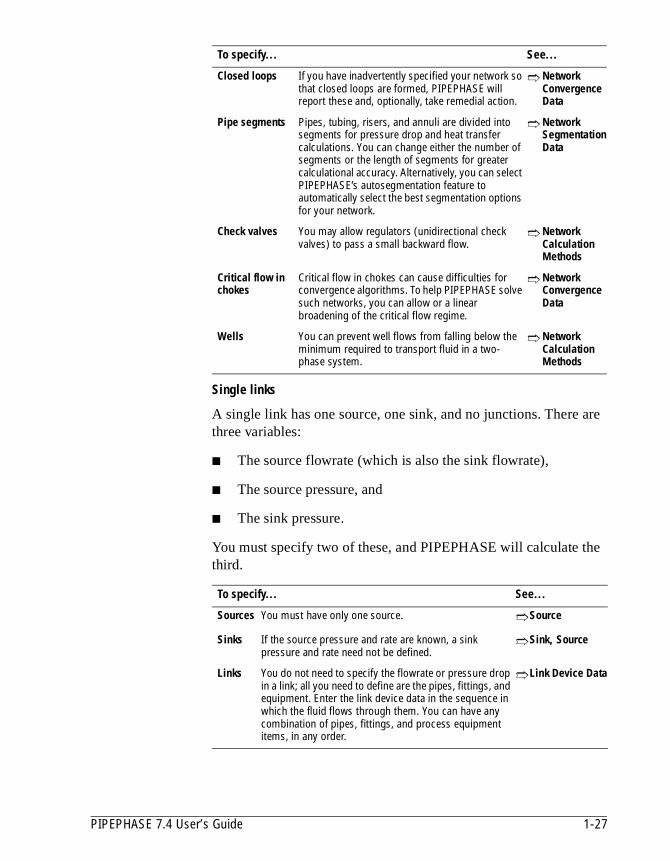
Single links
A single link has one source, one sink, and no junctions. There are three variables:
■ The source flowrate (which is also the sink flowrate),
■ The source pressure, and
■ The sink pressure.
You must specify two of these, and PIPEPHASE will calculate the third.
Closed loops If you have inadvertently specified your network so that closed loops are formed, PIPEPHASE will report these and, optionally, take remedial action.
➱ Network Convergence Data
Pipe segments Pipes, tubing, risers, and annuli are divided into segments for pressure drop and heat transfer calculations. You can change either the number of segments or the length of segments for greater calculational accuracy. Alternatively, you can select PIPEPHASE’s autosegmentation feature to automatically select the best segmentation options for your network.
➱ Network Segmentation Data
Check valves You may allow regulators (unidirectional check valves) to pass a small backward flow.
➱ Network Calculation Methods
Critical flow in chokes
Critical flow in chokes can cause difficulties for convergence algorithms. To help PIPEPHASE solve such networks, you can allow or a linear broadening of the critical flow regime.
➱ Network Convergence Data
Wells You can prevent well flows from falling below the minimum required to transport fluid in a two-phase system.
➱ Network Calculation Methods
To specify... See...
Sources You must have only one source. ➱Source
Sinks If the source pressure and rate are known, a sink pressure and rate need not be defined.
➱Sink, Source
Links You do not need to specify the flowrate or pressure drop in a link; all you need to define are the pipes, fittings, and equipment. Enter the link device data in the sequence in which the fluid flows through them. You can have any combination of pipes, fittings, and process equipment items, in any order.
➱Link Device Data
To specify... See...
PIPEPHASE 7.4 User’s Guide 1-27
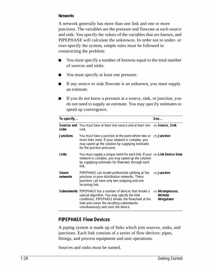
Networks
A network generally has more than one link and one or more junctions. The variables are the pressure and flowrate at each source and sink. You specify the values of the variables that are known, and PIPEPHASE will calculate the unknowns. In order not to under- or over-specify the system, simple rules must be followed in constructing the problem:
■ You must specify a number of knowns equal to the total number of sources and sinks.
■ You must specify at least one pressure.
■ If any source or sink flowrate is an unknown, you must supply an estimate.
■ If you do not know a pressure at a source, sink, or junction, you do not need to supply an estimate. You may specify estimates to speed up convergence.
PIPEPHASE Flow DevicesA piping system is made up of links which join sources, sinks, and junctions. Each link consists of a series of flow devices: pipes, fittings, and process equipment and unit operations.
Sources and sinks must be named.
To specify... See...
Sources and sinks
You must have at least one source and at least one sink.
➱ Source, Sink
Junctions You must have a junction at the point where two or more links meet. If your network is complex, you may speed up the solution by supplying estimates for the junction pressures.
➱ Junction
Links You must supply a unique name for each link. If your network is complex, you may speed up the solution by supplying estimates for flowrates through each link.
➱ Link Device Data
Steam networks
PIPEPHASE can model preferential splitting at Tee junctions in pure distribution networks. These junctions can have only two outgoing and one incoming link.
➱ Junction
Subnetworks PIPEPHASE has a number of devices that invoke a special algorithm. You may specify the inlet conditions; PIPEPHASE breaks the flowsheet at the inlet and solves the resulting subnetworks simultaneously and sizes the device.
➱ Mcompressor, Mchoke Mregulator
1-28 Getting Started
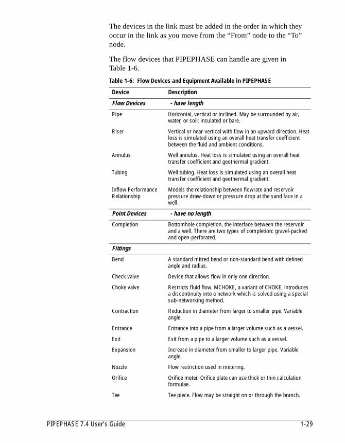
The devices in the link must be added in the order in which they occur in the link as you move from the “From” node to the “To” node.
The flow devices that PIPEPHASE can handle are given in Table 1-6.
Table 1-6: Flow Devices and Equipment Available in PIPEPHASE
Device Description
Flow Devices - have length
Pipe Horizontal, vertical or inclined. May be surrounded by air, water, or soil; insulated or bare.
Riser Vertical or near-vertical with flow in an upward direction. Heat loss is simulated using an overall heat transfer coefficient between the fluid and ambient conditions.
Annulus Well annulus. Heat loss is simulated using an overall heat transfer coefficient and geothermal gradient.
Tubing Well tubing. Heat loss is simulated using an overall heat transfer coefficient and geothermal gradient.
Inflow Performance Relationship
Models the relationship between flowrate and reservoir pressure draw-down or pressure drop at the sand face in a well.
Point Devices - have no length
Completion Bottomhole completion, the interface between the reservoir and a well. There are two types of completion: gravel-packed and open-perforated.
Fittings
Bend A standard mitred bend or non-standard bend with defined angle and radius.
Check valve Device that allows flow in only one direction.
Choke valve Restricts fluid flow. MCHOKE, a variant of CHOKE, introduces a discontinuity into a network which is solved using a special sub-networking method.
Contraction Reduction in diameter from larger to smaller pipe. Variable angle.
Entrance Entrance into a pipe from a larger volume such as a vessel.
Exit Exit from a pipe to a larger volume such as a vessel.
Expansion Increase in diameter from smaller to larger pipe. Variable angle.
Nozzle Flow restriction used in metering.
Orifice Orifice meter. Orifice plate can use thick or thin calculation formulae.
Tee Tee piece. Flow may be straight on or through the branch.
PIPEPHASE 7.4 User’s Guide 1-29
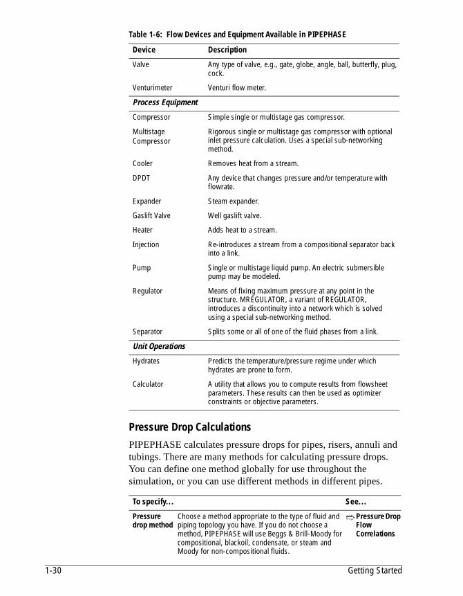
Pressure Drop CalculationsPIPEPHASE calculates pressure drops for pipes, risers, annuli and tubings. There are many methods for calculating pressure drops. You can define one method globally for use throughout the simulation, or you can use different methods in different pipes.
Valve Any type of valve, e.g., gate, globe, angle, ball, butterfly, plug, cock.
Venturimeter Venturi flow meter.
Process Equipment
Compressor Simple single or multistage gas compressor.
MultistageCompressor
Rigorous single or multistage gas compressor with optional inlet pressure calculation. Uses a special sub-networking method.
Cooler Removes heat from a stream.
DPDT Any device that changes pressure and/or temperature with flowrate.
Expander Steam expander.
Gaslift Valve Well gaslift valve.
Heater Adds heat to a stream.
Injection Re-introduces a stream from a compositional separator back into a link.
Pump Single or multistage liquid pump. An electric submersible pump may be modeled.
Regulator Means of fixing maximum pressure at any point in the structure. MREGULATOR, a variant of REGULATOR, introduces a discontinuity into a network which is solved using a special sub-networking method.
Separator Splits some or all of one of the fluid phases from a link.
Unit Operations
Hydrates Predicts the temperature/pressure regime under which hydrates are prone to form.
Calculator A utility that allows you to compute results from flowsheet parameters. These results can then be used as optimizer constraints or objective parameters.
To specify... See...
Pressure drop method
Choose a method appropriate to the type of fluid and piping topology you have. If you do not choose a method, PIPEPHASE will use Beggs & Brill-Moody for compositional, blackoil, condensate, or steam and Moody for non-compositional fluids.
➱ Pressure Drop Flow Correlations
Table 1-6: Flow Devices and Equipment Available in PIPEPHASE
Device Description
1-30 Getting Started
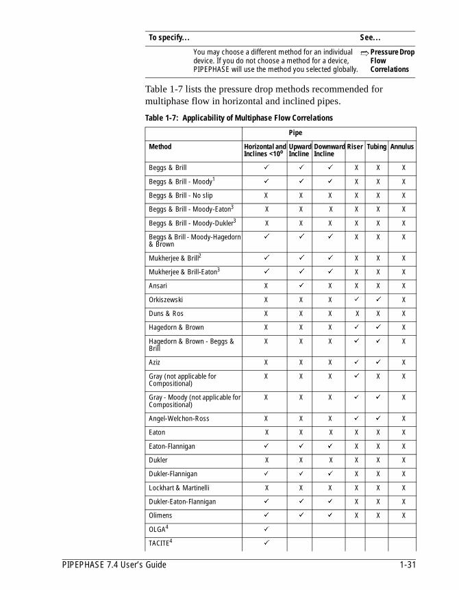
Table 1-7 lists the pressure drop methods recommended for multiphase flow in horizontal and inclined pipes.
You may choose a different method for an individual device. If you do not choose a method for a device, PIPEPHASE will use the method you selected globally.
➱ Pressure Drop Flow Correlations
Table 1-7: Applicability of Multiphase Flow Correlations
Pipe
Method Horizontal and Inclines <10o
Upward Incline
DownwardIncline
Riser Tubing Annulus
Beggs & Brill ä ä ä X X X
Beggs & Brill - Moody1ä ä ä X X X
Beggs & Brill - No slip X X X X X X
Beggs & Brill - Moody-Eaton3 X X X X X X
Beggs & Brill - Moody-Dukler3 X X X X X X
Beggs & Brill - Moody-Hagedorn & Brown
ä ä ä X X X
Mukherjee & Brill2 ä ä ä X X X
Mukherjee & Brill-Eaton3ä ä ä X X X
Ansari X ä X X X X
Orkiszewski X X X ä ä X
Duns & Ros X X X X X X
Hagedorn & Brown X X X ä ä X
Hagedorn & Brown - Beggs & Brill
X X X ä ä X
Aziz X X X ä ä X
Gray (not applicable for Compositional)
X X X ä X X
Gray - Moody (not applicable for Compositional)
X X X ä ä X
Angel-Welchon-Ross X X X ä ä X
Eaton X X X X X X
Eaton-Flannigan ä ä ä X X X
Dukler X X X X X X
Dukler-Flannigan ä ä ä X X X
Lockhart & Martinelli X X X X X X
Dukler-Eaton-Flannigan ä ä ä X X X
Olimens ä ä ä X X X
OLGA4ä
TACITE4ä
To specify... See...
PIPEPHASE 7.4 User’s Guide 1-31
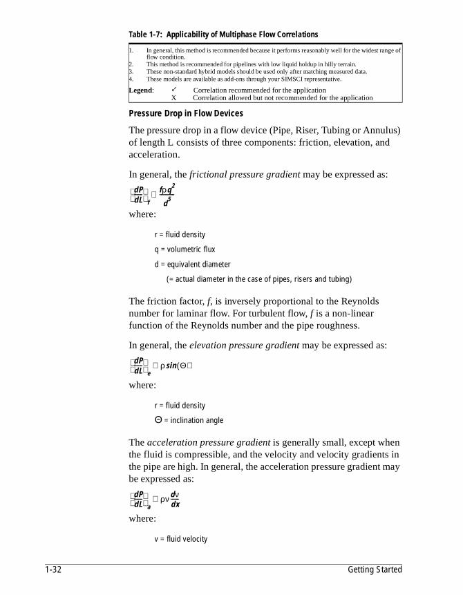
Pressure Drop in Flow Devices
The pressure drop in a flow device (Pipe, Riser, Tubing or Annulus) of length L consists of three components: friction, elevation, and acceleration.
In general, the frictional pressure gradient may be expressed as:
where:
The friction factor, f, is inversely proportional to the Reynolds number for laminar flow. For turbulent flow, f is a non-linear function of the Reynolds number and the pipe roughness.
In general, the elevation pressure gradient may be expressed as:
where:
The acceleration pressure gradient is generally small, except when the fluid is compressible, and the velocity and velocity gradients in the pipe are high. In general, the acceleration pressure gradient may be expressed as:
where:
1. In general, this method is recommended because it performs reasonably well for the widest range of flow condition.
2. This method is recommended for pipelines with low liquid holdup in hilly terrain.3. These non-standard hybrid models should be used only after matching measured data.4. These models are available as add-ons through your SIMSCI representative.
Legend: ä Correlation recommended for the applicationX Correlation allowed but not recommended for the application
r = fluid density
q = volumetric flux
d = equivalent diameter
(= actual diameter in the case of pipes, risers and tubing)
r = fluid density
Θ = inclination angle
v = fluid velocity
Table 1-7: Applicability of Multiphase Flow Correlations
dPdL------
f
fρq2
d5-----------∝
dPdL------
e
ρ Θ( )sin∝
dPdL------
a
ρνdνdx------∝
1-32 Getting Started

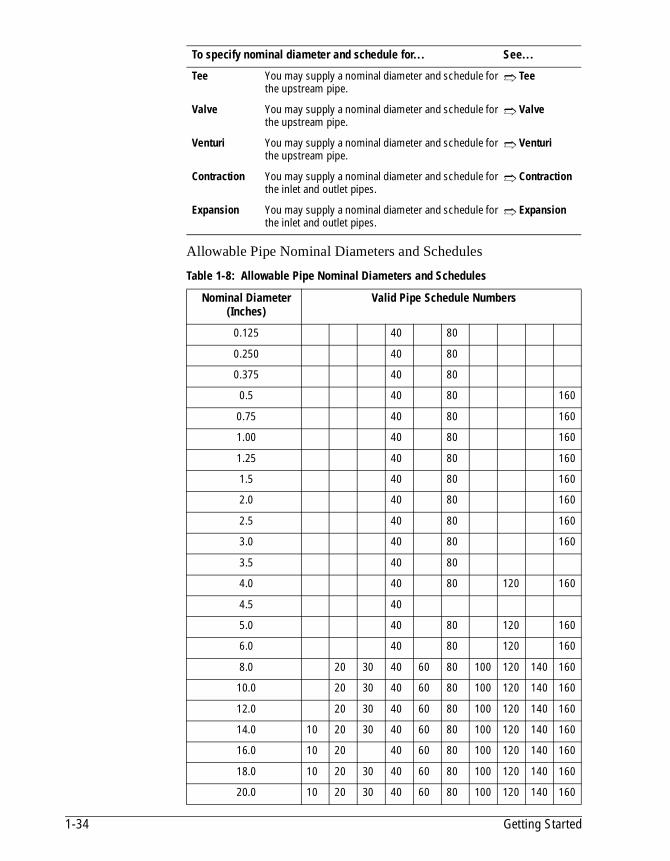
Nominal Diameter and Pipe Schedule
As an alternative to entering a pipe (or riser or tubing) inside diameter you can specify a nominal diameter and a schedule. PIPEPHASE has an internal database of standard nominal pipe sizes and pipe schedules; the allowed combinations of nominal diameter and schedule in this database are detailed in Table 1-8. You may supply your own database which PIPEPHASE will use instead of its own.
To specify... See...
Inside diameter and roughness
If the majority of your devices have the same inside diameter, you can specify a global inside diameter at the start of the simulation. Then you can override this value for those devices which do not conform to the default. Roughness can be specified also as a global parameter or for each device.
➱ Diameter Defaults
Inclined pipes You can specify an elevation change or depth for each device If the elevation change equals the length, the device is vertical. If you do not specify an elevation change, PIPEPHASE assumes that pipes are horizontal and that risers, annuli, and tubings are vertical.
➱ Pipe Riser Annulus Tubing
Acceleration terms
You may instruct PIPEPHASE to ignore the acceleration term in pressure drop calculations, if desired.
➱ Calculation Speedup Options
To specify nominal diameter and schedule for... See...
All devices as a global value
You may supply a nominal diameter and schedule that will be used for all the fittings in this table, unless overridden by data in the input to the fitting itself.
➱ Flow Devices Database Definition
Your pipes and fittings
You may create a database of nominal diameters and pipe schedules and have PIPEPHASE use it instead of its own internal database
➱ Flow Devices Database Definition
Pipe You may supply a nominal diameter and schedule. ➱ Pipe
Riser You may supply a nominal diameter and schedule. ➱ Riser
Tubing You may supply a nominal diameter and schedule. ➱ Tubing
Bend You may supply a nominal diameter and schedule. ➱ Bend
Entrance You may supply a nominal diameter and schedule for the downstream pipe.
➱ Entrance
Exit You may supply a nominal diameter and schedule for the upstream pipe.
➱ Exit
Nozzle You may supply a nominal diameter and schedule for the upstream pipe.
➱ Nozzle
Orifice You may supply a nominal diameter and schedule for the upstream pipe.
➱ Orifice
PIPEPHASE 7.4 User’s Guide 1-33
Allowable Pipe Nominal Diameters and Schedules
Tee You may supply a nominal diameter and schedule for the upstream pipe.
➱ Tee
Valve You may supply a nominal diameter and schedule for the upstream pipe.
➱ Valve
Venturi You may supply a nominal diameter and schedule for the upstream pipe.
➱ Venturi
Contraction You may supply a nominal diameter and schedule for the inlet and outlet pipes.
➱ Contraction
Expansion You may supply a nominal diameter and schedule for the inlet and outlet pipes.
➱ Expansion
Table 1-8: Allowable Pipe Nominal Diameters and Schedules
Nominal Diameter (Inches)
Valid Pipe Schedule Numbers
0.125 40 80
0.250 40 80
0.375 40 80
0.5 40 80 160
0.75 40 80 160
1.00 40 80 160
1.25 40 80 160
1.5 40 80 160
2.0 40 80 160
2.5 40 80 160
3.0 40 80 160
3.5 40 80
4.0 40 80 120 160
4.5 40
5.0 40 80 120 160
6.0 40 80 120 160
8.0 20 30 40 60 80 100 120 140 160
10.0 20 30 40 60 80 100 120 140 160
12.0 20 30 40 60 80 100 120 140 160
14.0 10 20 30 40 60 80 100 120 140 160
16.0 10 20 40 60 80 100 120 140 160
18.0 10 20 30 40 60 80 100 120 140 160
20.0 10 20 30 40 60 80 100 120 140 160
To specify nominal diameter and schedule for... See...
1-34 Getting Started
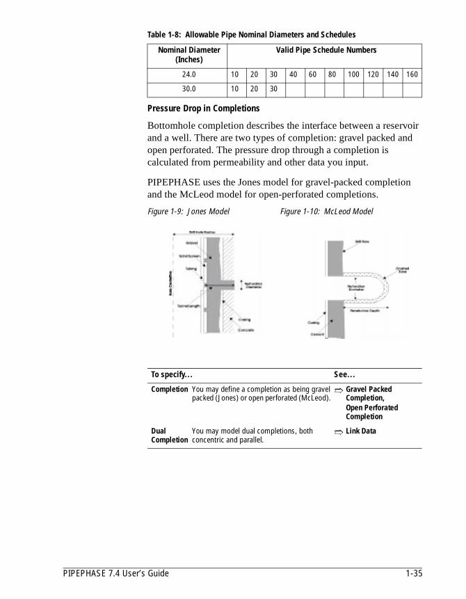
Pressure Drop in Completions
Bottomhole completion describes the interface between a reservoir and a well. There are two types of completion: gravel packed and open perforated. The pressure drop through a completion is calculated from permeability and other data you input.
PIPEPHASE uses the Jones model for gravel-packed completion and the McLeod model for open-perforated completions.
24.0 10 20 30 40 60 80 100 120 140 160
30.0 10 20 30
Figure 1-9: Jones Model Figure 1-10: McLeod Model
To specify... See...
Completion You may define a completion as being gravel packed (Jones) or open perforated (McLeod).
➱ Gravel Packed Completion,Open Perforated Completion
Dual Completion
You may model dual completions, both concentric and parallel.
➱ Link Data
Table 1-8: Allowable Pipe Nominal Diameters and Schedules
Nominal Diameter (Inches)
Valid Pipe Schedule Numbers
PIPEPHASE 7.4 User’s Guide 1-35

Pressure Drop in Fittings
The general form of the pressure drop equation is:
where:
∆P = pressure drop across the fitting
K = resistance coefficient/ K-factor
G = mass velocity (mass flowrate/flow area)
Φ = two-phase pressure drop multiplier
g = acceleration due to gravity
ρ = fluid density (equal to liquid density for two-phase flows)
To specify... See...
Bend, Tee,Valve
PIPEPHASE uses the generalized pressure drop equation with a resistance coefficient. For bends, tees, and valves, you can either supply the resistance coefficient directly or supply an equivalent length and have PIPEPHASE calculate the resistance coefficient as a function of the friction factor.
➱ Bend,Tee,Valve
Entrance Exit
For entrances and exits you can supply the resistance coefficient or use the default value.
➱ Entrance,Exit
Contraction, Expansion, Nozzle, Orifice, Venturi
For contractions, expansions, nozzles, orifices, and Venturimeters, you can supply the resistance coefficient or use the value that PIPEPHASE calculates from its built-in correlations. These correlations relate the resistance coefficient to the Reynolds number and specific fitting parameters such as orifice diameter, Venturi throat diameter, contraction and expansion angles, and nozzle diameter. For gas flow in nozzles, orifices, and Venturimeters, the specific heat ratio is also used in the calculation of the resistance coefficient.
➱ Nozzle, Expansion, Venturi, Contraction, Orifice
Choke The pressure drop for a choke is calculated by the orifice method for a single-phase fluid or by the Fortunati method for a two-phase fluid. You can supply a discharge coefficient or use the default value. MCHOKE, a variant of CHOKE which introduces a discontinuity into a network, uses the Fortunati model only.
➱ Choke Mchoke
Check Valve A valve that permits flow in one direction only. You can supply a resistance coefficient or use the default value.
➱ Check
Two-phase correction in fittings
The pressure drops for fittings are corrected for two-phase flow by using either the Homogeneous flow model or the Chisholm model. If you do not make a selection, PIPEPHASE will use the default method. You may supply values for the Chisholm parameters.
➱ Bend, Exit, Entrance, Valve, Tee, Contraction, Expansion, Nozzle, orifice, Venturi
∆P KG2Φ2gρ
--------------=
1-36 Getting Started

Equipment Items
PIPEPHASE simulates the change in fluid conditions across items of process equipment that typically appears in pipeline systems.
To specify... See...
Compressor A compressor imparts work to a gas. You supply either a known power or a known outlet pressure, and PIPEPHASE calculates the unknown parameter. You may impose a maximum value on the unknown parameter, and PIPEPHASE will constrain the calculations according to whichever parameter is limiting. Alternatively, you can supply a curve of flowrate against head. You may also supply an adiabatic efficiency as either a constant or a curve against head. The exit temperature is then determined by energy balance. If you specify more than one stage, PIPEPHASE interprets the curve to be for each stage; any maximum power you specify is over all of the stages rather than for each individual stage.
➱ Compressor
You can also reference the compressor curve to a previously defined performance curve.
➱ Compressor Curve Data, Compressor Performance Curves
Multispeed Compressor
You can specify different compressor curves for up to five compressor speeds.
➱ Compressor Curve Data
Multistage Compressor
In a multistage compressor you may specify different parameters – curves, efficiencies, etc.– for different stages. You may have multiple compressor trains, each train with multiple stages. You may have interstage scrubbers with downstream re-injection and interstage coolers and piping losses. You may specify the compressor’s inlet pressure. When you do this, PIPEPHASE invokes a special algorithm which breaks the flowsheet at the compressor inlet and solves the resulting subnetworks so that the pressures match at the interface.
➱ Mcompressor
Cooler The cooler removes heat from the system. You supply either a known exit temperature or known duty of the unit, and PIPEPHASE will calculate the unknown parameter. You may impose a maximum (for duty) or minimum (for temperature) value on the unknown parameter, and PIPEPHASE will constrain calculations according to whichever parameter is limiting.
➱ Cooler
Steam Expander
The expander models the expansion of steam from a high pressure to a low pressure. You may specify the power required, or the pressure drop or the pressure ratio. If the unit is in a spur link, you may alternatively specify the outlet pressure.
➱ Expander
Gaslift Valve This unit simulates the presence of a gaslift valve as part of a well link. You must define the PVT properties of the lift gas.
➱ Gaslift Valve, Fluid Property Data
PIPEPHASE 7.4 User’s Guide 1-37
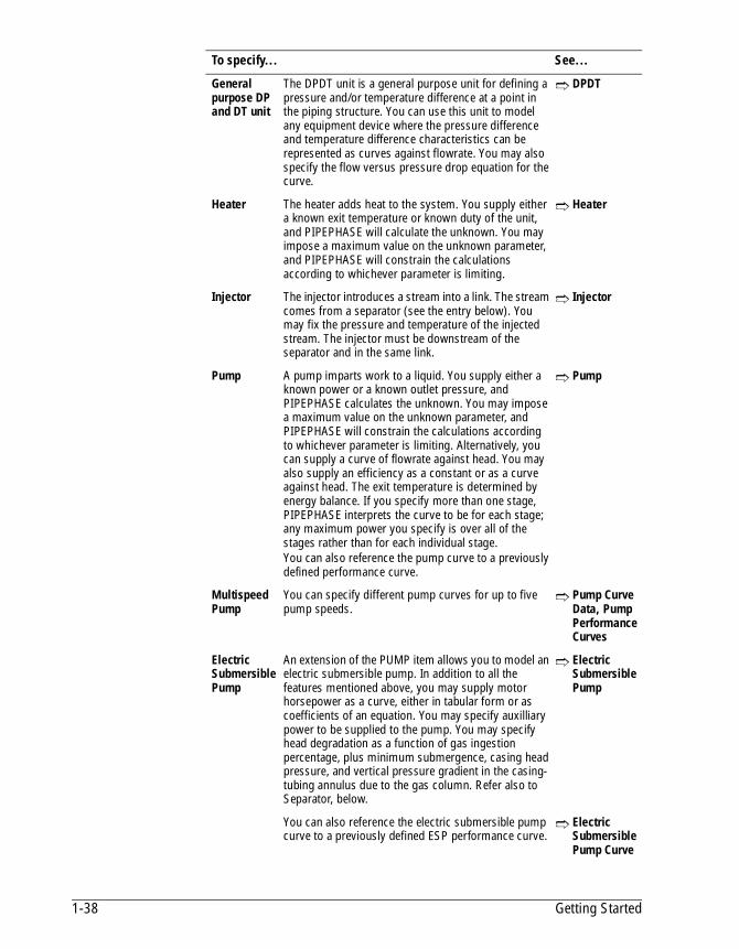
General purpose DP and DT unit
The DPDT unit is a general purpose unit for defining a pressure and/or temperature difference at a point in the piping structure. You can use this unit to model any equipment device where the pressure difference and temperature difference characteristics can be represented as curves against flowrate. You may also specify the flow versus pressure drop equation for the curve.
➱ DPDT
Heater The heater adds heat to the system. You supply either a known exit temperature or known duty of the unit, and PIPEPHASE will calculate the unknown. You may impose a maximum value on the unknown parameter, and PIPEPHASE will constrain the calculations according to whichever parameter is limiting.
➱ Heater
Injector The injector introduces a stream into a link. The stream comes from a separator (see the entry below). You may fix the pressure and temperature of the injected stream. The injector must be downstream of the separator and in the same link.
➱ Injector
Pump A pump imparts work to a liquid. You supply either a known power or a known outlet pressure, and PIPEPHASE calculates the unknown. You may impose a maximum value on the unknown parameter, and PIPEPHASE will constrain the calculations according to whichever parameter is limiting. Alternatively, you can supply a curve of flowrate against head. You may also supply an efficiency as a constant or as a curve against head. The exit temperature is determined by energy balance. If you specify more than one stage, PIPEPHASE interprets the curve to be for each stage; any maximum power you specify is over all of the stages rather than for each individual stage.You can also reference the pump curve to a previously defined performance curve.
➱ Pump
Multispeed Pump
You can specify different pump curves for up to five pump speeds.
➱ Pump Curve Data, Pump Performance Curves
Electric Submersible Pump
An extension of the PUMP item allows you to model an electric submersible pump. In addition to all the features mentioned above, you may supply motor horsepower as a curve, either in tabular form or as coefficients of an equation. You may specify auxilliary power to be supplied to the pump. You may specify head degradation as a function of gas ingestion percentage, plus minimum submergence, casing head pressure, and vertical pressure gradient in the casing-tubing annulus due to the gas column. Refer also to Separator, below.
➱ Electric Submersible Pump
You can also reference the electric submersible pump curve to a previously defined ESP performance curve.
➱ Electric Submersible Pump Curve
To specify... See...
1-38 Getting Started
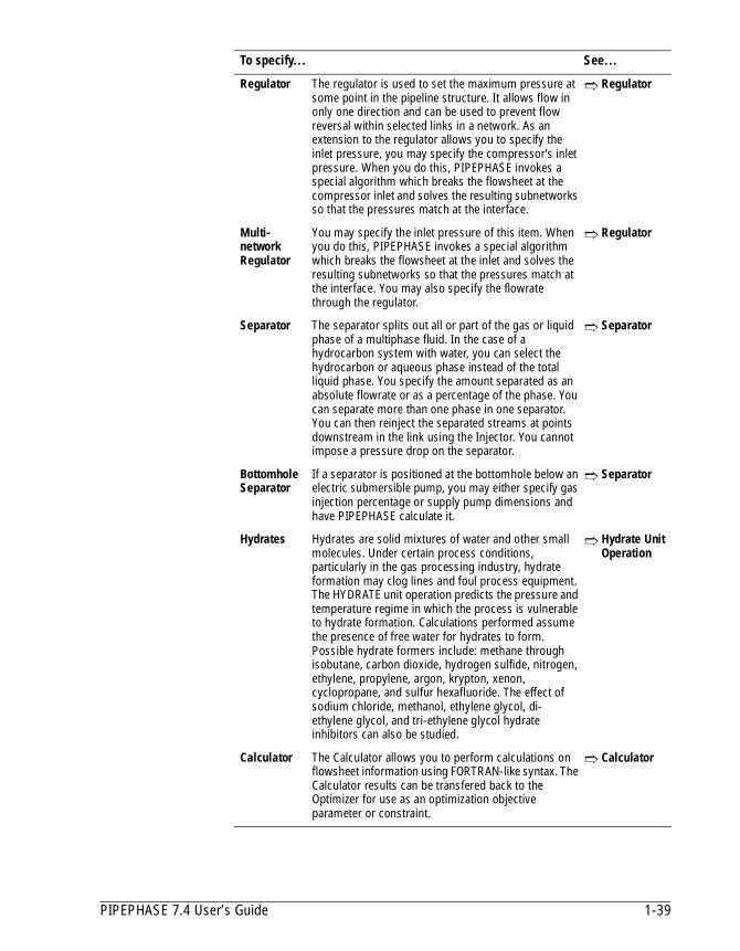
Regulator The regulator is used to set the maximum pressure at some point in the pipeline structure. It allows flow in only one direction and can be used to prevent flow reversal within selected links in a network. As an extension to the regulator allows you to specify the inlet pressure, you may specify the compressor’s inlet pressure. When you do this, PIPEPHASE invokes a special algorithm which breaks the flowsheet at the compressor inlet and solves the resulting subnetworks so that the pressures match at the interface.
➱ Regulator
Multi-network Regulator
You may specify the inlet pressure of this item. When you do this, PIPEPHASE invokes a special algorithm which breaks the flowsheet at the inlet and solves the resulting subnetworks so that the pressures match at the interface. You may also specify the flowrate through the regulator.
➱ Regulator
Separator The separator splits out all or part of the gas or liquid phase of a multiphase fluid. In the case of a hydrocarbon system with water, you can select the hydrocarbon or aqueous phase instead of the total liquid phase. You specify the amount separated as an absolute flowrate or as a percentage of the phase. You can separate more than one phase in one separator. You can then reinject the separated streams at points downstream in the link using the Injector. You cannot impose a pressure drop on the separator.
➱ Separator
Bottomhole Separator
If a separator is positioned at the bottomhole below an electric submersible pump, you may either specify gas injection percentage or supply pump dimensions and have PIPEPHASE calculate it.
➱ Separator
Hydrates Hydrates are solid mixtures of water and other small molecules. Under certain process conditions, particularly in the gas processing industry, hydrate formation may clog lines and foul process equipment. The HYDRATE unit operation predicts the pressure and temperature regime in which the process is vulnerable to hydrate formation. Calculations performed assume the presence of free water for hydrates to form. Possible hydrate formers include: methane through isobutane, carbon dioxide, hydrogen sulfide, nitrogen, ethylene, propylene, argon, krypton, xenon, cyclopropane, and sulfur hexafluoride. The effect of sodium chloride, methanol, ethylene glycol, di-ethylene glycol, and tri-ethylene glycol hydrate inhibitors can also be studied.
➱ Hydrate Unit Operation
Calculator The Calculator allows you to perform calculations on flowsheet information using FORTRAN-like syntax. The Calculator results can be transfered back to the Optimizer for use as an optimization objective parameter or constraint.
➱ Calculator
To specify... See...
PIPEPHASE 7.4 User’s Guide 1-39

Heat Transfer Calculations
PIPEPHASE performs an energy balance on pipes, risers, tubing, and annuli. The heat transfer depends on the fluid temperature, properties, and flowrate, the temperature and properties of the surrounding medium, and the heat transfer coefficient between the fluid and the medium. PIPEPHASE does not model heat transfer to the surroundings for fittings and equipment devices (point devices).
The general equation for heat transfer from a flow device is:
where:
The overall heat transfer coefficient either is input or may be calculated from the constituent film coefficients and geometries.
For risers and annuli you must specify an overall heat transfer coefficient.
For a pipe or tubing you may supply an overall coefficient or you may request detailed heat transfer calculations. Detailed heat transfer calculations are invoked when you input any one of the parameters required to carry out the calculations.
Detailed Heat Transfer in Pipes and Tubing
For a pipe surrounded by soil, water, or air, you define the medium properties (and velocity of water or air). For a buried pipe, you enter the buried depth.
For tubings you enter data that describe the properties of the annuli and casings between the outside of the tubing and the inside of the hole.
Q = rate of heat transfer per unit length
U = overall heat transfer coefficient
A = outside surface area per unit length
DT = temperature difference between bulk fluid and outside medium
To specify... See...
Pipes and Tubing
You may specify an overall coefficient or the properties of the surrounding medium. You can supply these values globally for all devices or for individual devices. You also supply the ambient temperature or geothermal gradient.
➱ Global Defaults Pipe Tubing
Q UA∆T=
1-40 Getting Started

e ed.
e
e
ks.
Sphering or PiggingPIPEPHASE’s sphering calculations predict the quantity of liquidformed when a multiphase fluid flows in a pipeline and determinthe size of the liquid slug that is pushed out when the pipe is pigg
Sphering calculations can only be carried out for single links. Thlaunching station is at the inlet of a pipe. You may have intermediate launching stations; a sphere is launched from a pipwhen the previous sphere(s) reach the inlet of that pipe.
Reservoirs and Inflow Performance RelationshipsUsing PIPEPHASE, you can examine the effect of reservoir conditions on the performance of wells and downstream networYou can also investigate the implications of declining reservoir pressure and production rate and shut-in wells when a user-specified maximum water cut or gas-oil ratio is exceeded.
Annuli and Risers
You specify the overall heat transfer coefficient and the geothermal gradient. You can supply these values globally for all devices or for individual devices.
➱ Global Defaults Annulus Riser
Isothermal calculations
For non-compositional gas or liquid fluid models, you may suppress heat transfer calculations for individual flow devices.
➱ Pipe Tubing Annulus Riser
To specify... See...
Calculation type You must specify that you want to do a sphering simulation.
➱ Network Calculation Methods
Fluid type The fluid must be compositional and both gas and liquid should be present to obtain realistic results.
➱ Simulation Definition
Time Increments You may override the default time step used in the McDonald-Baker successive steady-state calculation method.
➱ Network Calculation Methods
Structure Data You may have only PIPE devices. You identify a pipe with a launching station by specifying a sphere diameter for the pipe. The first launching station must be in the first pipe of the link.
➱ Pipe
To specify... See...
PIPEPHASE 7.4 User’s Guide 1-41
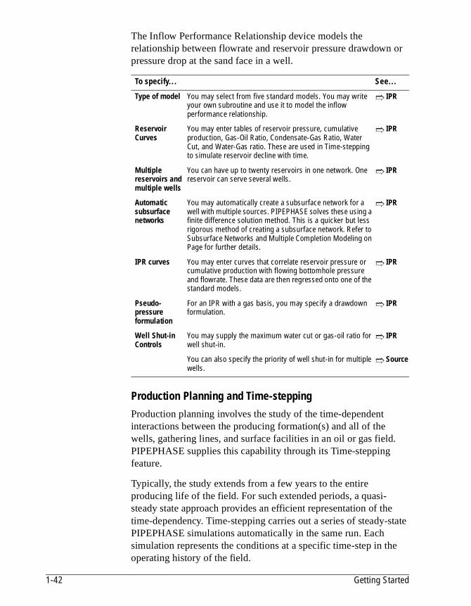
The Inflow Performance Relationship device models the relationship between flowrate and reservoir pressure drawdown or pressure drop at the sand face in a well.
Production Planning and Time-steppingProduction planning involves the study of the time-dependent interactions between the producing formation(s) and all of the wells, gathering lines, and surface facilities in an oil or gas field. PIPEPHASE supplies this capability through its Time-stepping feature.
Typically, the study extends from a few years to the entire producing life of the field. For such extended periods, a quasi-steady state approach provides an efficient representation of the time-dependency. Time-stepping carries out a series of steady-state PIPEPHASE simulations automatically in the same run. Each simulation represents the conditions at a specific time-step in the operating history of the field.
To specify... See...
Type of model You may select from five standard models. You may write your own subroutine and use it to model the inflow performance relationship.
➱ IPR
Reservoir Curves
You may enter tables of reservoir pressure, cumulative production, Gas-Oil Ratio, Condensate-Gas Ratio, Water Cut, and Water-Gas ratio. These are used in Time-stepping to simulate reservoir decline with time.
➱ IPR
Multiple reservoirs and multiple wells
You can have up to twenty reservoirs in one network. One reservoir can serve several wells.
➱ IPR
Automatic subsurface networks
You may automatically create a subsurface network for a well with multiple sources. PIPEPHASE solves these using a finite difference solution method. This is a quicker but less rigorous method of creating a subsurface network. Refer to Subsurface Networks and Multiple Completion Modeling on Page for further details.
➱ IPR
IPR curves You may enter curves that correlate reservoir pressure or cumulative production with flowing bottomhole pressure and flowrate. These data are then regressed onto one of the standard models.
➱ IPR
Pseudo-pressure formulation
For an IPR with a gas basis, you may specify a drawdown formulation.
➱ IPR
Well Shut-in Controls
You may supply the maximum water cut or gas-oil ratio for well shut-in.
➱ IPR
You can also specify the priority of well shut-in for multiple wells.
➱ Source
1-42 Getting Started
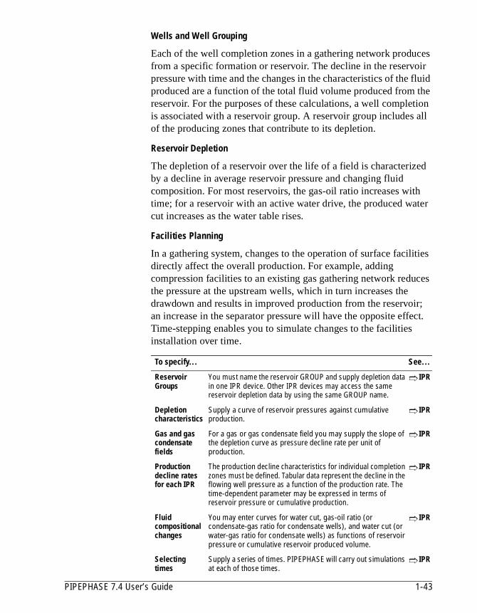
Wells and Well Grouping
Each of the well completion zones in a gathering network produces from a specific formation or reservoir. The decline in the reservoir pressure with time and the changes in the characteristics of the fluid produced are a function of the total fluid volume produced from the reservoir. For the purposes of these calculations, a well completion is associated with a reservoir group. A reservoir group includes all of the producing zones that contribute to its depletion.
Reservoir Depletion
The depletion of a reservoir over the life of a field is characterized by a decline in average reservoir pressure and changing fluid composition. For most reservoirs, the gas-oil ratio increases with time; for a reservoir with an active water drive, the produced water cut increases as the water table rises.
Facilities Planning
In a gathering system, changes to the operation of surface facilities directly affect the overall production. For example, adding compression facilities to an existing gas gathering network reduces the pressure at the upstream wells, which in turn increases the drawdown and results in improved production from the reservoir; an increase in the separator pressure will have the opposite effect. Time-stepping enables you to simulate changes to the facilities installation over time.
To specify... See...
Reservoir Groups
You must name the reservoir GROUP and supply depletion data in one IPR device. Other IPR devices may access the same reservoir depletion data by using the same GROUP name.
➱ IPR
Depletion characteristics
Supply a curve of reservoir pressures against cumulative production.
➱ IPR
Gas and gas condensate fields
For a gas or gas condensate field you may supply the slope of the depletion curve as pressure decline rate per unit of production.
➱ IPR
Production decline rates for each IPR
The production decline characteristics for individual completion zones must be defined. Tabular data represent the decline in the flowing well pressure as a function of the production rate. The time-dependent parameter may be expressed in terms of reservoir pressure or cumulative production.
➱ IPR
Fluid compositional changes
You may enter curves for water cut, gas-oil ratio (or condensate-gas ratio for condensate wells), and water cut (or water-gas ratio for condensate wells) as functions of reservoir pressure or cumulative reservoir produced volume.
➱ IPR
Selecting times
Supply a series of times. PIPEPHASE will carry out simulations at each of those times.
➱ IPR
PIPEPHASE 7.4 User’s Guide 1-43
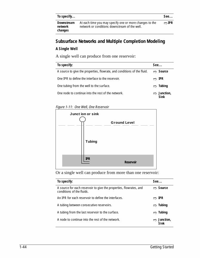
Subsurface Networks and Multiple Completion ModelingA Single Well
A single well can produce from one reservoir:
Figure 1-11: One Well, One Reservoir
Or a single well can produce from more than one reservoir:
Downstream network changes
At each time you may specify one or more changes to the network or conditions downstream of the well.
➱ IPR
To specify: See...
A source to give the properties, flowrate, and conditions of the fluid. ➱ Source
One IPR to define the interface to the reservoir. ➱ IPR
One tubing from the well to the surface. ➱ Tubing
One node to continue into the rest of the network. ➱ Junction, Sink
To specify: See...
A source for each reservoir to give the properties, flowrates, and conditions of the fluids.
➱ Source
An IPR for each reservoir to define the interfaces. ➱ IPR
A tubing between consecutive reservoirs. ➱ Tubing
A tubing from the last reservoir to the surface. ➱ Tubing
A node to continue into the rest of the network. ➱ Junction, Sink
To specify... See...
Tubing
Ground Level
Junction or sink
ReservoirIPR
1-44 Getting Started

Figure 1-12: One Well, More Than One Reservoir
More Than One Well
You may have more than one well in a PIPEPHASE run. The wells may all use one reservoir. In this case, information for the reservoir data is entered in one IPR and accessed from other IPRs using the GROUP name.
Multiple Completions
In PIPEPHASE you may model a multiple completion rigorously:
To specify: See...
A source for each completion to give the properties, flowrates, and conditions of the fluids.
➱ Source
An IPR for each completion to define the interfaces. ➱ IPR
Tubing and junctions to form the network between completions. ➱ Tubing
A tubing from the last completion to the surface. ➱ Tubing
A node to continue into the rest of the network. ➱ Junction, Sink
Tubing
Ground Level
Reservoir
Tubing
Reservoir
Junction or sink
IPR
IPR
Subsurface junction
PIPEPHASE 7.4 User’s Guide 1-45
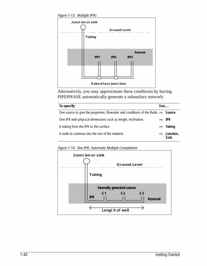
Figure 1-13: Multiple IPRs
Alternatively, you may approximate these conditions by having PIPEPHASE automatically generate a subsurface network:
Figure 1-14: One IPR, Automatic Multiple Completions
To specify: See...
One source to give the properties, flowrates and conditions of the fluids. ➱ Source
One IPR with physical dimensions such as length, inclination. ➱ IPR
A tubing from the IPR to the surface. ➱ Tubing
A node to continue into the rest of the network. ➱ Junction, Sink
ReservoirIPR1 IPR2 IPR3
Tubing
Ground Level
Junction or sink
Subsurface junctions
Reservoir
Length of well
S 1 S 2 S 3Internally generated sources
IPR
Tubing
Ground Level
Junction or sink
1-46 Getting Started

Case Studies
The Case Study option provides the facility to perform parametric studies and to print multiple problem solutions in a single computer run. Case studies are always performed after the base case problem has been solved. If the base case problem cannot be solved for any reason, then no case studies are performed. Each case study analysis is performed based on the cumulative changes to the flowsheet up to that time.
Case studies are an efficient means of obtaining solutions for multiple scenarios to a given problem and result in large savings in both computer time and cost. For problems requiring iterative solutions, the converged results of the last solution are used as the starting values for the next run. This can result in large computer time savings in runs involving large networks, where it typically takes several iterations to move from the initial pressure estimates to the final converged solution.
There is no limit on the number of changes you can make per case study or on the total number of case studies that may be in a given run. The cumulative changes up to a given case study run may be erased and the original base case restored at any time.
Since the case studies are performed sequentially in the order you input, it is best to make changes in an orderly manner, proceeding from high values to low values or low values to high values, but not in a random order. This enhances convergence and minimizes total computer time. See Chapter 4, Input Reference, Table 4-46.
Global Changes
You may change one parameter in the entire problem using a global command. You do this by supplying the type of parameter you want to change, its old value, and the new value. Only those specified parameters with that old value will then be changed.
The items to which this type of change can be applied are identified in Table 4-46, Chapter 4, Input Reference.
PIPEPHASE 7.4 User’s Guide 1-47

Individual Changes
Source, sink, and device parameters may be changed individually. You must specify a name for each source, sink, or device where a parameter change is desired,
To... See...
Add descriptive text
You can add one line of description for each case study.
➱ Simulation Description
Make changes You can change any of the parameters in Table 3-7, either globally or on individual flow elements.
➱ Case Study Changes
You can restore the base case at any time. ➱ Case Study Changes
Table 1-9: Changes allowed in Case Studies
Flow Device Parameter Type of Change
Pipe LENGTHECHGIDROUGHNESSUTAMBIENTFCODE
Global IndividualGlobal IndividualGlobal IndividualGlobal IndividualGlobal IndividualGlobal IndividualGlobal Individual
Riser IDROUGHNESSUFCODE
Global IndividualGlobal IndividualGlobal IndividualGlobal Individual
Tubing IDROUGHNESSUFCODETGRAD
Global IndividualGlobal IndividualGlobal IndividualGlobal IndividualGlobal Individual
Annulus IDANNODTUBROUGHNESSUFCODETGRAD
Global IndividualGlobal IndividualGlobal IndividualGlobal IndividualGlobal IndividualGlobal Individual
Compressor/Pump
POWERPRESSUREEFFICIENCYSTAGES
Global IndividualGlobal IndividualGlobal IndividualGlobal Individual
Heater/Cooler DUTYTOUTDP
Global IndividualGlobal IndividualGlobal Individual
Choke IDCOEFFICIENT
Global IndividualGlobal Individual
Sales RATE Global Individual
1-48 Getting Started
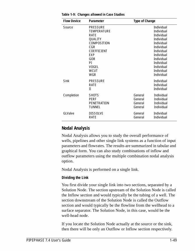
Nodal AnalysisNodal Analysis allows you to study the overall performance of wells, pipelines and other single link systems as a function of input parameters and flowrates. The results are summarized in tabular and graphical form. You can also study combinations of inflow and outflow parameters using the multiple combination nodal analysis option.
Nodal Analysis is performed on a single link.
Dividing the Link
You first divide your single link into two sections, separated by a Solution Node. The section upstream of the Solution Node is called the Inflow section and would typically be the tubing of a well. The section downstream of the Solution Node is called the Outflow section and would typically be the flowline from the wellhead to a surface separator. The Solution Node, in this case, would be the well-head node.
If you locate the Solution Node actually at the source or the sink, then there will be only an Outflow or Inflow section respectively.
Source PRESSURETEMPERATURERATEQUALITYCOMPOSITIONCGRCOEFFICIENTEXPGORPIVOGELWCUTWGR
IndividualIndividualIndividualIndividualIndividualIndividualIndividualIndividualIndividualIndividualIndividualIndividualIndividual
Sink PRESSURERATEII
IndividualIndividualIndividual
Completion SHOTSPERFPENETRATIONTUNNEL
General IndividualGeneral IndividualGeneral IndividualGeneral Individual
GLValve DISSOLVERATE
General IndividualGeneral Individual
Table 1-9: Changes allowed in Case Studies
Flow Device Parameter Type of Change
PIPEPHASE 7.4 User’s Guide 1-49

If you do not want to vary any parameters in either the Inflow section or the Outflow section, simply omit these sections. Obviously, a Nodal Analysis cannot be carried out without at least one of these sections.
Selecting Parameters and Flowrates
You then select a parameter in the Inflow section and a parameter in the Outflow section. Typical parameters would be reservoir pressure (for Inflow) and pipe ID (for Outflow). You may enter up to five values for each of these parameters. Each combination of Inflow parameter value and Outflow parameter value represents an operating point of the system. This means that there may be up to 25 operating points.
The parameters you select must have values supplied in the base case input data.
Finally, you define up to ten flowrates.
Nodal Results
PIPEPHASE calculates the flowrates and Solution Node pressures corresponding to each operating point and prints them out in the form of tables and plots. The flowrates you input must span all the flowrates at which you expect the operating points to occur.
Grouping Parameters
As an extension to the Nodal Analysis feature, PIPEPHASE allows you to group a number of variables into one nodal parameter. For example, you may define an Outflow parameter as a combination of pump power, pipe ID and heater temperature. Each of the five values of the Outflow parameter would now be a combination of the corresponding values of each of the contributing variables.
1-50 Getting Started

Thus you might define that the first value of the Outflow parameter is the combination of 25KW pump power with 30 mm pipe ID and 400 K; the second 30KW, 40 mm and 310 K; the third 35KW, 50 mm and 350 K; and so on.
To... See...
Add descriptive text
You can add one line of description for each of the Inflow and Outflow sections.
➱ Simulation Description
Define the Solution Node
You must define a Solution Node which comes between the Inflow and Outflow sections. If you want the Solution Node to be at the flowing bottomhole of an injection well, use BOTTOMHOLE. If you want to locate the Solution Node at the outlet of the last device and want to use Sink pressure as a variable parameter, use SINK.
➱ Link Device Data, Nodal Analysis
Define the parameter(s)
You must define at least one Inflow or Outflow parameter for PIPEPHASE to change. The parameters that are accessible are divided into seven categories, as defined in the table below. If you want to define a nodal parameter as a group of variables, you may combine up to ten variables within one Category. You may not combine variables in different categories.
➱ Nodal Analysis Parameters
Study multiple combinations of parameters
You can specify up to four — two inflow and two outflow — parameters for the multiple combinations option. You can then supply up to five values of each parameter. PIPEPHASE will combine each of the up to five values of an inflow or outflow parameter with each of the up to five values of the second inflow or outflow parameter and so on and will present the results of the analysis of the combined variables.
➱ Nodal Analysis
Table 1-10: Variables Available to Nodal AnalysisCategory Device Variable
Category 1 - Source SOURCE NAMEPRESSURECOEFFICIENTEXPPIVOGEL
Category 2 - Sink SINK NAMEPRESIICOEFFEXP
Category 3 - Devices PIPE NAMEIDROUGHNESSUFLOWEFF
PIPEPHASE 7.4 User’s Guide 1-51
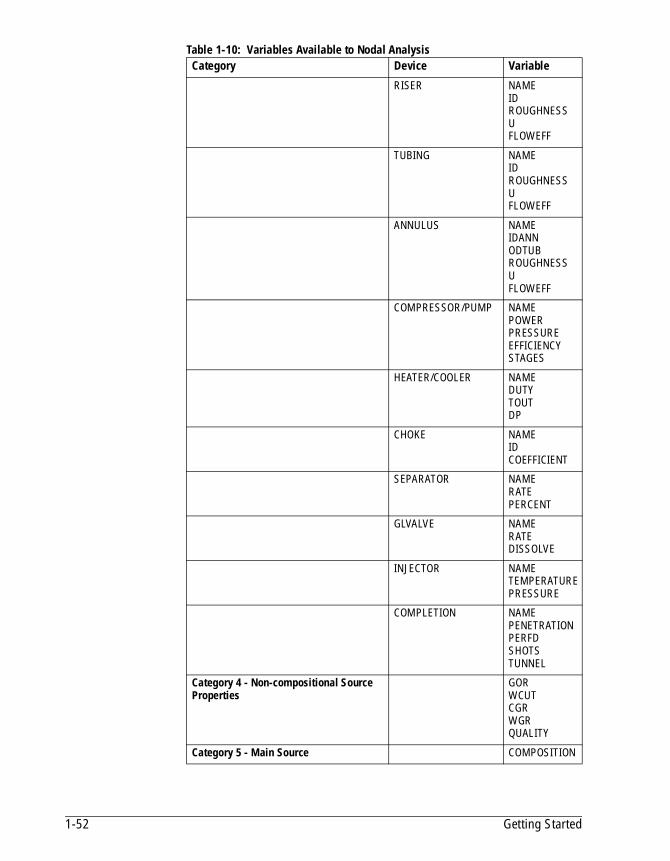
RISER NAMEIDROUGHNESSUFLOWEFF
TUBING NAMEIDROUGHNESSUFLOWEFF
ANNULUS NAMEIDANNODTUBROUGHNESSUFLOWEFF
COMPRESSOR/PUMP NAMEPOWERPRESSUREEFFICIENCYSTAGES
HEATER/COOLER NAMEDUTYTOUTDP
CHOKE NAMEIDCOEFFICIENT
SEPARATOR NAMERATEPERCENT
GLVALVE NAMERATEDISSOLVE
INJECTOR NAMETEMPERATUREPRESSURE
COMPLETION NAMEPENETRATIONPERFDSHOTSTUNNEL
Category 4 - Non-compositional Source Properties
GORWCUTCGRWGRQUALITY
Category 5 - Main Source COMPOSITION
Table 1-10: Variables Available to Nodal AnalysisCategory Device Variable
1-52 Getting Started
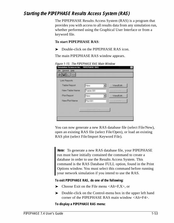
Starting the PIPEPHASE Results Access System (RAS)The PIPEPHASE Results Access System (RAS) is a program that provides you with access to all results data from any simulation run, whether performed using the Graphical User Interface or from a keyword file.
To start PIPEPHASE RAS:
➤ Double-click on the PIPEPHASE RAS icon.
The main PIPEPHASE RAS window appears.
Figure 1-15: The PIPEPHASE RAS Main Window
You can now generate a new RAS database file (select File/New), open an existing RAS file (select File/Open), or load an existing RAS plot (select File/Import Keyword File).
To exit PIPEPHASE RAS, do one of the following:
➤ Choose Exit on the File menu <Alt+F,X>, or
➤ Double-click on the Control-menu box in the upper left hand corner of the PIPEPHASE RAS main window <Alt+F4>.
To display a PIPEPHASE RAS menu:
Note: To generate a new RAS database file, your PIPEPHASE run must have initially contained the command to create a database in order to use the Results Access System. This command is the RAS Database FULL option, found in the Print Options window. You must select this command before running your network simulation if you intend to use the RAS.
PIPEPHASE 7.4 User’s Guide 1-53
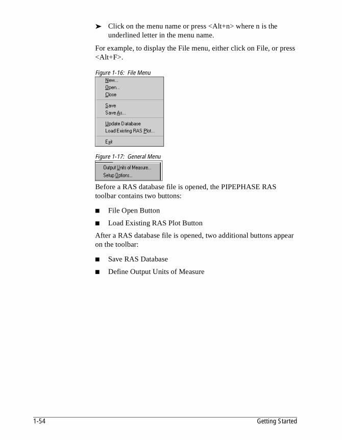
➤ Click on the menu name or press <Alt+n> where n is the underlined letter in the menu name.
For example, to display the File menu, either click on File, or press <Alt+F>.
Figure 1-16: File Menu
Figure 1-17: General Menu
Before a RAS database file is opened, the PIPEPHASE RAS toolbar contains two buttons:
■ File Open Button
■ Load Existing RAS Plot Button
After a RAS database file is opened, two additional buttons appear on the toolbar:
■ Save RAS Database
■ Define Output Units of Measure
1-54 Getting Started
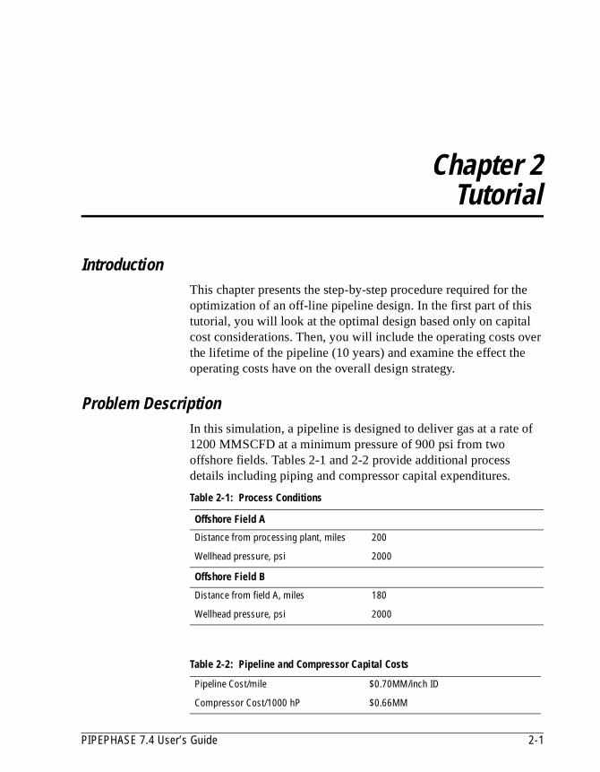
Chapter 2Tutorial
IntroductionThis chapter presents the step-by-step procedure required for the optimization of an off-line pipeline design. In the first part of this tutorial, you will look at the optimal design based only on capital cost considerations. Then, you will include the operating costs over the lifetime of the pipeline (10 years) and examine the effect the operating costs have on the overall design strategy.
Problem DescriptionIn this simulation, a pipeline is designed to deliver gas at a rate of 1200 MMSCFD at a minimum pressure of 900 psi from two offshore fields. Tables 2-1 and 2-2 provide additional process details including piping and compressor capital expenditures.
Table 2-1: Process Conditions
Offshore Field A
Distance from processing plant, miles 200
Wellhead pressure, psi 2000
Offshore Field B
Distance from field A, miles 180
Wellhead pressure, psi 2000
Table 2-2: Pipeline and Compressor Capital Costs
Pipeline Cost/mile $0.70MM/inch ID
Compressor Cost/1000 hP $0.66MM
PIPEPHASE 7.4 User’s Guide 2-1

The overall capital cost is the sum of the cost of purchasing and laying pipe and purchasing the compressors.
The overall capital cost is therefore a linear function of the ID of the two pipeline segments and compressor power:
PIPEPHASE optimizes the design to minimize the overall capital costs by varying the pipe diameters and the sizes of the compressors at the two platforms. Apart from the delivery target, there are three additional design and operating constraints that must be taken into consideration:
■ Pipe sizes are available only in sizes 24"-40" with a maximum operating pressure of 2475 psi.
■ Due to limited space on each platform, the maximum capacity of each compressor is 50000 hP.
■ Both pipeline sections must be built as the capacity of the plat-form for field A is inadequate to meet the overall delivery requirement.
The overall network is shown in Figure 2-1.
Figure 2-1: Tutorial Problem
Pipe Costs (MM$) = Cost of Pipe from Field 1 + Cost of Pipe from Field 2
= 0.70*200*IDPipe 1 + 0.70*180*IDPipe 2
= 140*IDPipe 1 + 126*IDPipe 2
Compressor Cost (MM$) = 6.6E-4*wCompr 1 + 6.6E-4*wCompr 2
Capital Cost = 140*IDPipe 1 + 126*IDPipe 2 + 6.6E-4*wCompr 1 + 6.6E-4*wCompr 2
2-2 Tutorial
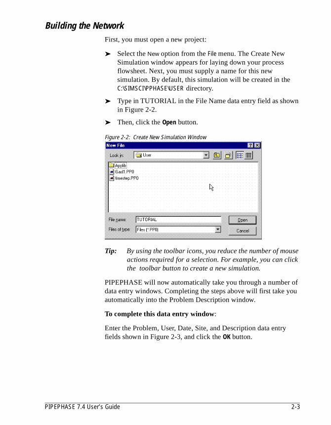
Building the NetworkFirst, you must open a new project:
➤ Select the New option from the File menu. The Create New Simulation window appears for laying down your process flowsheet. Next, you must supply a name for this new simulation. By default, this simulation will be created in the C:\SIMSCI\PPHASE\USER directory.
➤ Type in TUTORIAL in the File Name data entry field as shown in Figure 2-2.
➤ Then, click the Open button.
Figure 2-2: Create New Simulation Window
Tip: By using the toolbar icons, you reduce the number of mouse actions required for a selection. For example, you can click the toolbar button to create a new simulation.
PIPEPHASE will now automatically take you through a number of data entry windows. Completing the steps above will first take you automatically into the Problem Description window.
To complete this data entry window:
Enter the Problem, User, Date, Site, and Description data entry fields shown in Figure 2-3, and click the OK button.
PIPEPHASE 7.4 User’s Guide 2-3
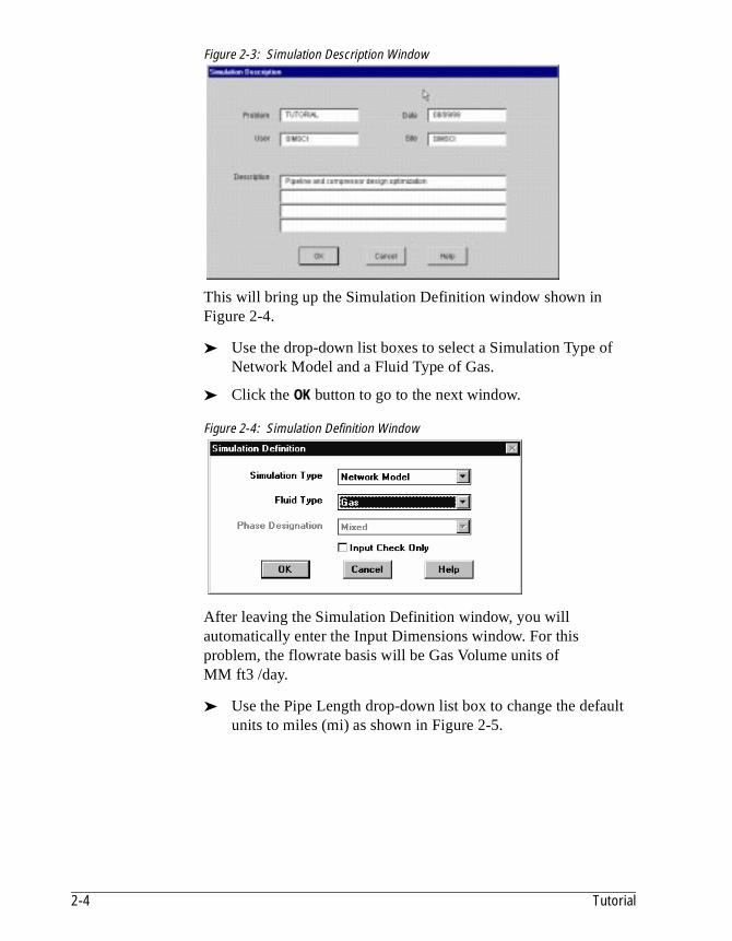
Figure 2-3: Simulation Description Window
This will bring up the Simulation Definition window shown in Figure 2-4.
➤ Use the drop-down list boxes to select a Simulation Type of Network Model and a Fluid Type of Gas.
➤ Click the OK button to go to the next window.
Figure 2-4: Simulation Definition Window
After leaving the Simulation Definition window, you will automatically enter the Input Dimensions window. For this problem, the flowrate basis will be Gas Volume units of MM ft3 /day.
➤ Use the Pipe Length drop-down list box to change the default units to miles (mi) as shown in Figure 2-5.
2-4 Tutorial
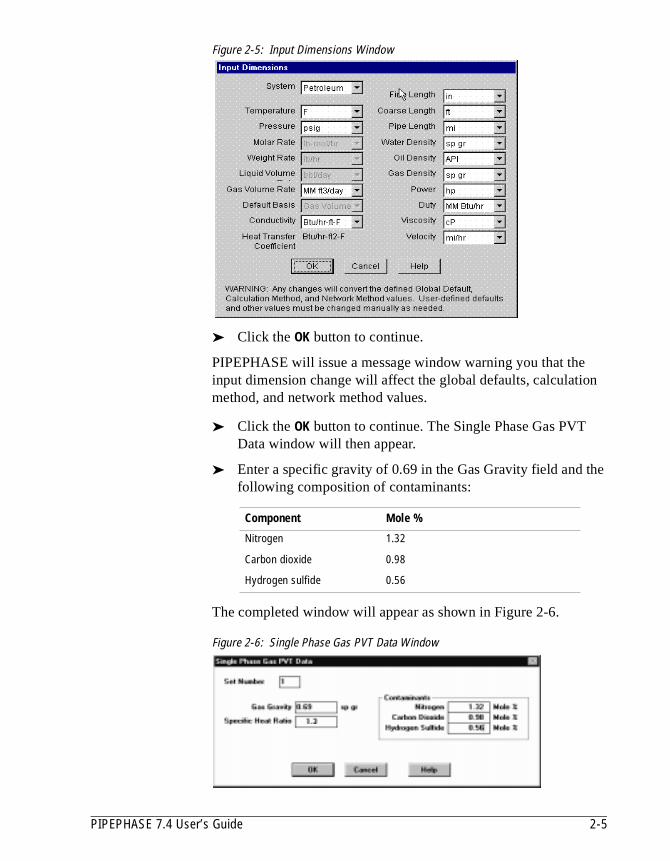
Figure 2-5: Input Dimensions Window
➤ Click the OK button to continue.
PIPEPHASE will issue a message window warning you that the input dimension change will affect the global defaults, calculation method, and network method values.
➤ Click the OK button to continue. The Single Phase Gas PVT Data window will then appear.
➤ Enter a specific gravity of 0.69 in the Gas Gravity field and the following composition of contaminants:
The completed window will appear as shown in Figure 2-6.
Figure 2-6: Single Phase Gas PVT Data Window
Component Mole %
Nitrogen 1.32
Carbon dioxide 0.98
Hydrogen sulfide 0.56
PIPEPHASE 7.4 User’s Guide 2-5

➤ Click the OK button to continue. The Fluid Property Data window will appear as shown in Figure 2-7.
Figure 2-7: Fluid Property Data
You must now create a second property data set.
➤ Click the New button. This brings up the Single Phase Gas PVT Data window with Set Number already set to 2.
➤ Enter a specific gravity of 0.701 in the Gas Gravity field and the following composition of contaminants:
The completed window will appear as shown in Figure 2-8.
Figure 2-8: Single Phase Gas PVT Data Window
➤ Click the OK button. The Fluid Property Data window will appear as shown in Figure 2-9.
Component Mole %
Nitrogen 1.11
Carbon dioxide 0.88
Hydrogen sulfide 0.24
2-6 Tutorial
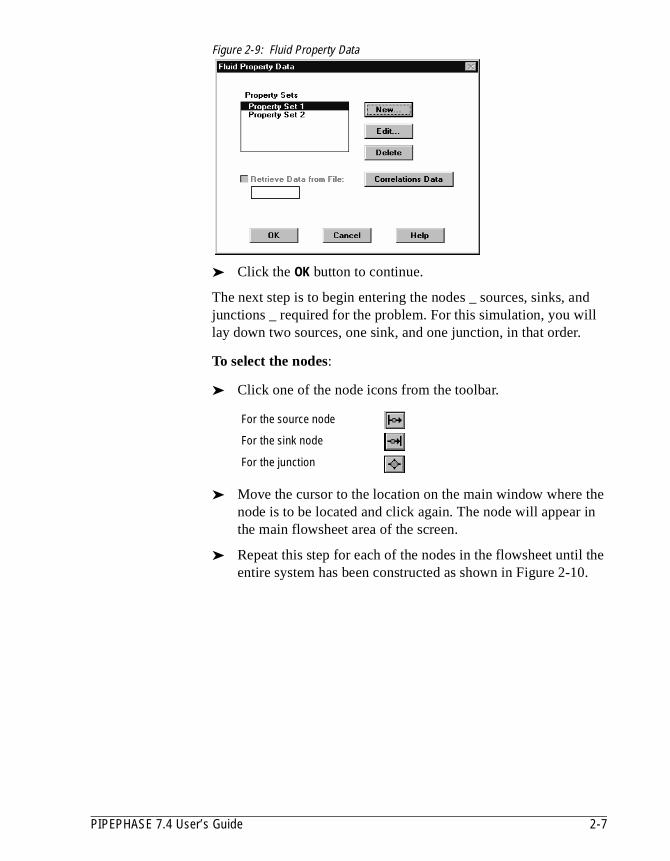
Figure 2-9: Fluid Property Data
➤ Click the OK button to continue.
The next step is to begin entering the nodes _ sources, sinks, and junctions _ required for the problem. For this simulation, you will lay down two sources, one sink, and one junction, in that order.
To select the nodes:
➤ Click one of the node icons from the toolbar.
➤ Move the cursor to the location on the main window where the node is to be located and click again. The node will appear in the main flowsheet area of the screen.
➤ Repeat this step for each of the nodes in the flowsheet until the entire system has been constructed as shown in Figure 2-10.
For the source node
For the sink node
For the junction
PIPEPHASE 7.4 User’s Guide 2-7

e as
.
Figure 2-10: PIPEPHASE Main Window
Tip: For very large systems, multiple nodes may be placed by holding down the Shift key and clicking on each desired location for a given node.
All of the source and sink nodes placed on the screen should be bordered in red indicating that user input is required for that node.
After all of the nodes have been placed, the next step is to connect the nodes into a logical flow network.
To connect two nodes:
➤ Click on a source or junction (“From” node) with the left mouse button. A red square will appear on the node, and thborder of the node will turn green to indicate that the node hbeen selected.
➤ Next, click inside the square with the left mouse button and,while holding the mouse button down, drag the cursor to another junction or sink (“To” node).
Note: Once a node has been placed, it may be moved by simply clicking on the node with the left mouse button, holding it down, and dragging the node to a new location.
Note: If you have added the nodes in the stated order of sources, sink, followed by the junction, the sources will be labeled S001 and S002, the sink, D003, and the junction, J004
2-8 Tutorial
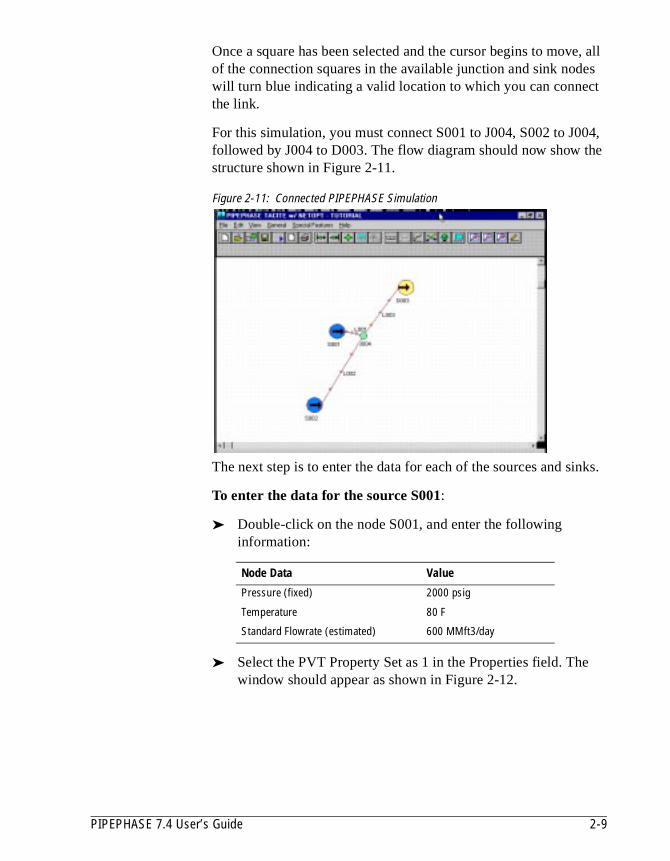
Once a square has been selected and the cursor begins to move, all of the connection squares in the available junction and sink nodes will turn blue indicating a valid location to which you can connect the link.
For this simulation, you must connect S001 to J004, S002 to J004, followed by J004 to D003. The flow diagram should now show the structure shown in Figure 2-11.
Figure 2-11: Connected PIPEPHASE Simulation
The next step is to enter the data for each of the sources and sinks.
To enter the data for the source S001:
➤ Double-click on the node S001, and enter the following information:
➤ Select the PVT Property Set as 1 in the Properties field. The window should appear as shown in Figure 2-12.
Node Data Value
Pressure (fixed) 2000 psig
Temperature 80 F
Standard Flowrate (estimated) 600 MMft3/day
PIPEPHASE 7.4 User’s Guide 2-9
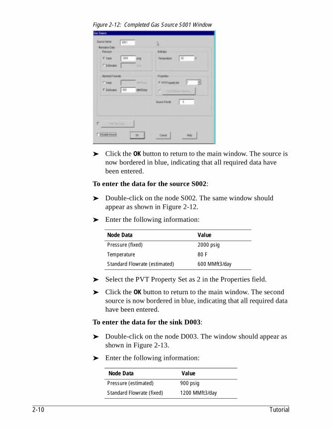
Figure 2-12: Completed Gas Source S001 Window
➤ Click the OK button to return to the main window. The source is now bordered in blue, indicating that all required data have been entered.
To enter the data for the source S002:
➤ Double-click on the node S002. The same window should appear as shown in Figure 2-12.
➤ Enter the following information:
➤ Select the PVT Property Set as 2 in the Properties field.
➤ Click the OK button to return to the main window. The second source is now bordered in blue, indicating that all required data have been entered.
To enter the data for the sink D003:
➤ Double-click on the node D003. The window should appear as shown in Figure 2-13.
➤ Enter the following information:
Node Data Value
Pressure (fixed) 2000 psig
Temperature 80 F
Standard Flowrate (estimated) 600 MMft3/day
Node Data Value
Pressure (estimated) 900 psig
Standard Flowrate (fixed) 1200 MMft3/day
2-10 Tutorial
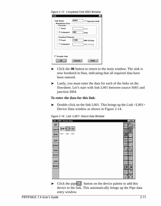
d
Figure 2-13: Completed Sink D003 Window
➤ Click the OK button to return to the main window. The sink is now bordered in blue, indicating that all required data have been entered.
➤ Lastly, you must enter the data for each of the links on the flowsheet. Let’s start with link L001 between source S001 anjunction J004.
To enter the data for this link:
➤ Double-click on the link L001. This brings up the Link <L001>Device Data window as shown in Figure 2-14.
Figure 2-14: Link <L001> Device Data Window
➤ Click the pipe button on the device palette to add this device to the link. This automatically brings up the Pipe dataentry window.
PIPEPHASE 7.4 User’s Guide 2-11
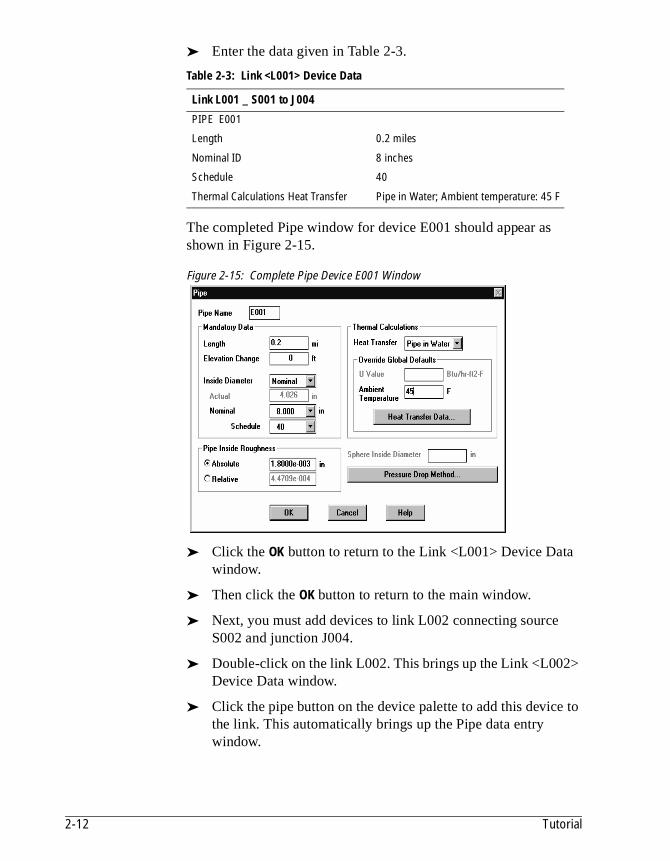
➤ Enter the data given in Table 2-3.
The completed Pipe window for device E001 should appear as shown in Figure 2-15.
Figure 2-15: Complete Pipe Device E001 Window
➤ Click the OK button to return to the Link <L001> Device Data window.
➤ Then click the OK button to return to the main window.
➤ Next, you must add devices to link L002 connecting source S002 and junction J004.
➤ Double-click on the link L002. This brings up the Link <L002> Device Data window.
➤ Click the pipe button on the device palette to add this device to the link. This automatically brings up the Pipe data entry window.
Table 2-3: Link <L001> Device Data
Link L001 _ S001 to J004
PIPE E001
Length 0.2 miles
Nominal ID 8 inches
Schedule 40
Thermal Calculations Heat Transfer Pipe in Water; Ambient temperature: 45 F
2-12 Tutorial
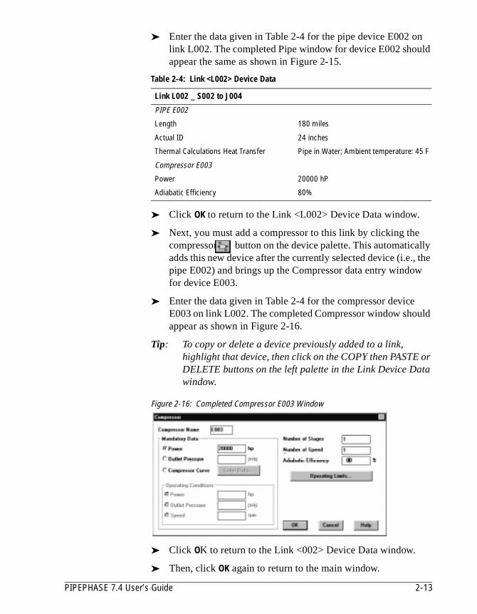
➤ Enter the data given in Table 2-4 for the pipe device E002 on link L002. The completed Pipe window for device E002 should appear the same as shown in Figure 2-15.
➤ Click OK to return to the Link <L002> Device Data window.
➤ Next, you must add a compressor to this link by clicking the compressor button on the device palette. This automatically adds this new device after the currently selected device (i.e., the pipe E002) and brings up the Compressor data entry window for device E003.
➤ Enter the data given in Table 2-4 for the compressor device E003 on link L002. The completed Compressor window should appear as shown in Figure 2-16.
Tip: To copy or delete a device previously added to a link, highlight that device, then click on the COPY then PASTE or DELETE buttons on the left palette in the Link Device Data window.
Figure 2-16: Completed Compressor E003 Window
➤ Click OK to return to the Link <002> Device Data window.
➤ Then, click OK again to return to the main window.
Table 2-4: Link <L002> Device Data
Link L002 _ S002 to J004
PIPE E002
Length 180 miles
Actual ID 24 inches
Thermal Calculations Heat Transfer Pipe in Water; Ambient temperature: 45 F
Compressor E003
Power 20000 hP
Adiabatic Efficiency 80%
PIPEPHASE 7.4 User’s Guide 2-13

rs.
gs
➤ Using the data given in Table 2-5, repeat the above steps for link L003 connecting junction J004 to sink D003.The main window will now appear as shown in Figure 2-18.
Figure 2-17: PIPEPHASE Main Window
Let’s save the data entered so far.
➤ Click the Save button on the toolbar, or select the File/Save menu option.
Entering Optimization DataNow, you must define the design constraints, coefficients for theobjective function, decision variables, and optimization paramete
➤ Click the Network Optimization Data button on the toolbar, orselect the General/Optimization Data menu option. This brinup the Network Optimization Data window.
➤ Check the Enable Network Optimization check box.
Table 2-5: Link <L003> Device Data
Link L003 _ J004 to D003
PIPE E004
Length 200 miles
Actual ID 35 inches
Thermal Calculations Heat Transfer Pipe in Water; Ambient temperature: 45 F
Compressor E005
Power 25000 hP
Adiabatic Efficiency 80%
2-14 Tutorial

➤ In the Objective data entry field, select the Minimize Objective Function radio button as shown in Figure 2-18.
Figure 2-18: Network Optimization Window
➤ Now, you must define the objective parameters by clicking on the Objective Parameters button to bring up the Network Optimization Objective Parameters window.
As discussed previously, the overall capital cost is a linear function of the ID of the two pipeline segments and compressor power:
There are therefore four objective parameters for this optimization problem as shown in Table 2-6.
To enter the first objective parameter:
➤ In the Network Optimization Objective Parameters window, click the Add button. This brings up the Define Objective Parameter window.
➤ Select the Link Name radio button in the Node/Device/Calculator Name field.
➤ Select link L003 from the Link Name drop-down list box.
Capital Cost = 140*IDPipe 1 + 126*IDPipe 2 + 6.6E-4*wCompr 1 + 6.6E-4*wCompr 2
Table 2-6: Objective Parameters
Link Description Coefficient in Objective Function
L003 Pipe E004 Inside Diameter, ID 140
L002 Pipe E002 Inside Diameter, ID 126
L003 Compressor E005 Power, w 6.6e-4
L002 Compressor E003 Power, w 6.6e-4
PIPEPHASE 7.4 User’s Guide 2-15

➤ Select Pipe from the Device Type drop-down list box. By default, PIPEPHASE will display the correct device name, E004.
➤ Select Inside Diameter from the Parameter drop-down list box.
➤ Type in 140 in the Correlation Coefficient data entry field as shown in Figure 2-19.
Figure 2-19: Define Objective Parameter Window
➤ Repeat for the other three objective parameters using the data in Table 2-6.
Tip: For the Compressor objective parameters, select Available Power from the Parameters drop-down list box in the Define Objective Parameter window.
➤ The completed Network Optimization Objective Parameters window is shown in Figure 2-21.
Figure 2-20: Network Optimization Objective Parameters Window
2-16 Tutorial

➤ Click the OK button to return to the Network Optimization Data window.
➤ Next you must define the decision variables.
There are four decision variables for this optimization problem as shown in Table 2-7 below.
To enter the first decision variable:
➤ In the Network Optimization Data window, click the Add button. This brings up the Define Decision Variable window.
➤ Select the Link Name radio button in the Node/Device Name field.
➤ Select link L003 from the Link Name drop-down list box.
➤ Select Pipe from the Device Type drop-down list box. By default, PIPEPHASE will display the correct device name, E004.
➤ Select Inside Diameter from the Parameter drop-down list box.
➤ Click the Limits button. This brings up the Optimizer Variable Limits window as shown in Figure 2-21.
➤ In the Variable Lower Limit field, enter a value of 24 for Mechanical Limit (Absolute Value).
➤ In the Variable Upper Limit field, enter a value of 48 for Mechanical Limit (Absolute Value).
Table 2-7: Decision Variables
Link Description Limits Relative Perturbation
L003 Pipe E004 Internal Diameter, ID 24”<ID<48” -
L002 Pipe E002 Internal Diameter, ID 24”<ID<48” -
L002 Compressor E003 Power, w 0 hP<w<50000 hP 0.001
L003 Compressor E005 Power, w 0 hp<w<50000 hP 0.001
PIPEPHASE 7.4 User’s Guide 2-17

Figure 2-21: Optimizer Variable Limits Window
➤ Click the OK button to return to the Define Decision Variable window.
➤ Then, click the OK again to return to the Network Optimization Data window.
➤ Repeat for the other three decision variables using the data in Table 2-7 above.
Tip: For the Compressor decision variables, select Available Power from the Parameters drop-down list box in the Define Decision Variable window.
The Network Optimization Data window should now appear as shown in Figure 2-22.
Figure 2-22: Network Optimization Data Window
2-18 Tutorial
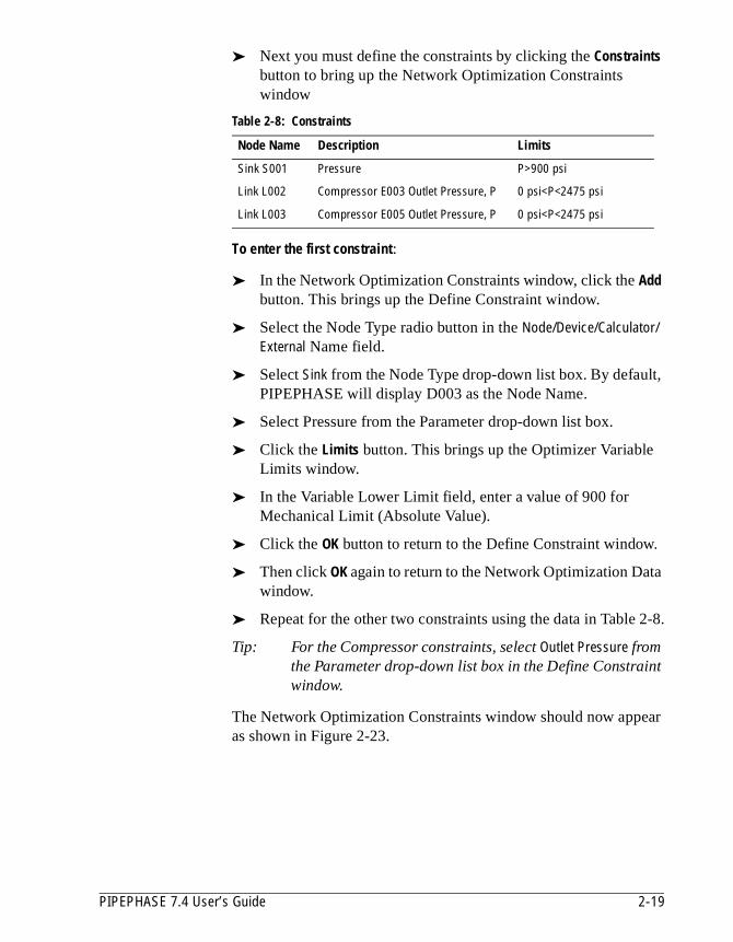
➤ Next you must define the constraints by clicking the Constraints button to bring up the Network Optimization Constraints window
To enter the first constraint:
➤ In the Network Optimization Constraints window, click the Add button. This brings up the Define Constraint window.
➤ Select the Node Type radio button in the Node/Device/Calculator/External Name field.
➤ Select Sink from the Node Type drop-down list box. By default, PIPEPHASE will display D003 as the Node Name.
➤ Select Pressure from the Parameter drop-down list box.
➤ Click the Limits button. This brings up the Optimizer Variable Limits window.
➤ In the Variable Lower Limit field, enter a value of 900 for Mechanical Limit (Absolute Value).
➤ Click the OK button to return to the Define Constraint window.
➤ Then click OK again to return to the Network Optimization Data window.
➤ Repeat for the other two constraints using the data in Table 2-8.
Tip: For the Compressor constraints, select Outlet Pressure from the Parameter drop-down list box in the Define Constraint window.
The Network Optimization Constraints window should now appear as shown in Figure 2-23.
Table 2-8: Constraints
Node Name Description Limits
Sink S001 Pressure P>900 psi
Link L002 Compressor E003 Outlet Pressure, P 0 psi<P<2475 psi
Link L003 Compressor E005 Outlet Pressure, P 0 psi<P<2475 psi
PIPEPHASE 7.4 User’s Guide 2-19
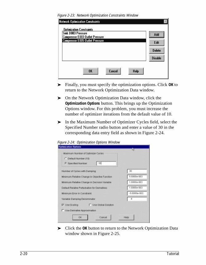
Figure 2-23: Network Optimization Constraints Window
➤ Finally, you must specify the optimization options. Click OK to return to the Network Optimization Data window.
➤ On the Network Optimization Data window, click the Optimization Options button. This brings up the Optimization Options window. For this problem, you must increase the number of optimizer iterations from the default value of 10.
➤ In the Maximum Number of Optimizer Cycles field, select the Specified Number radio button and enter a value of 30 in the corresponding data entry field as shown in Figure 2-24.
Figure 2-24: Optimization Options Window
➤ Click the OK button to return to the Network Optimization Data window shown in Figure 2-25.
2-20 Tutorial

Figure 2-25: Network Optimization Data Window
➤ Then, click the OK button again to return to the main PIPEPHASE window.
➤ Select the File/Save menu option to save the simulation date entered so far.
Specifying Print OptionsBefore you can run the simulation, you must specify the print options for the output report and save the simulation.
➤ Select the General/Print Options menu option from the main PIPEPHASE window. This brings up the Print Options window as shown in Figure 2-28.
➤ Select the FULL option from the RAS Database drop-down list box.
➤ Select the NONE option from the Input Reprint drop-down list box.
➤ Select the FULL option from the Device Detail drop-down list box. The completed Print Options window should appear as shown in Figure 2-27.
Note: You must turn off the input reprint, select that all device details be printed (the FULL option), and generate a database for the Results Access System (RAS).
PIPEPHASE 7.4 User’s Guide 2-21
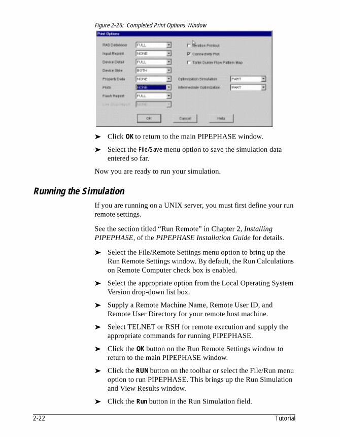
ns
em
u n
Figure 2-26: Completed Print Options Window
➤ Click OK to return to the main PIPEPHASE window.
➤ Select the File/Save menu option to save the simulation data entered so far.
Now you are ready to run your simulation.
Running the SimulationIf you are running on a UNIX server, you must first define your run remote settings.
See the section titled “Run Remote” in Chapter 2, Installing PIPEPHASE, of the PIPEPHASE Installation Guide for details.
➤ Select the File/Remote Settings menu option to bring up theRun Remote Settings window. By default, the Run Calculatioon Remote Computer check box is enabled.
➤ Select the appropriate option from the Local Operating SystVersion drop-down list box.
➤ Supply a Remote Machine Name, Remote User ID, and Remote User Directory for your remote host machine.
➤ Select TELNET or RSH for remote execution and supply theappropriate commands for running PIPEPHASE.
➤ Click the OK button on the Run Remote Settings window to return to the main PIPEPHASE window.
➤ Click the RUN button on the toolbar or select the File/Run menoption to run PIPEPHASE. This brings up the Run Simulatioand View Results window.
➤ Click the Run button in the Run Simulation field.
2-22 Tutorial
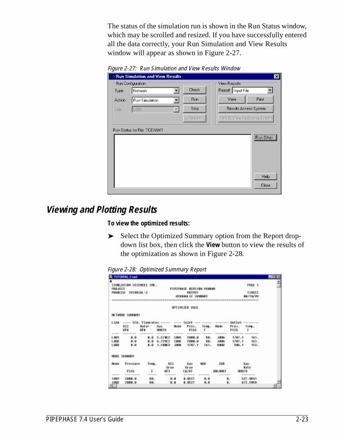
The status of the simulation run is shown in the Run Status window, which may be scrolled and resized. If you have successfully entered all the data correctly, your Run Simulation and View Results window will appear as shown in Figure 2-27.
Figure 2-27: Run Simulation and View Results Window
Viewing and Plotting ResultsTo view the optimized results:
➤ Select the Optimized Summary option from the Report drop-down list box, then click the View button to view the results of the optimization as shown in Figure 2-28.
Figure 2-28: Optimized Summary Report
PIPEPHASE 7.4 User’s Guide 2-23

Table 2-9 summarizes the optimal solution for this simulation.
Using the RAS to Plot ResultsPIPEPHASE includes a powerful utility called the Results Access System (RAS) that allows you to plot the results of your optimization run.
➤ First, find and launch the RAS program. The main PIPEPHASE RAS window appears as shown in Figure 2-29.
Figure 2-29: PIPEPHASE RAS Window
➤ Next, select the File/New menu option.
➤ Select the TUTORIAL.RAS database file.
Table 2-9: Optimized Solution Results
Minimum Capital Cost $7,581 MM
Pipe, E002 ID 24”
Pipe, E004 ID 32.1”
Compressor, E003 Power 45,873 hP
Compressor, E005 Power 50,000 hP
Source, S001 Flowrate 524 MMSCFD
Source, S002 Flowrate 676 MMSCFD
Note: Under Windows 3.1, double-click on the PIPEPHASE RAS icon located in the SIMSCI group window.
2-24 Tutorial
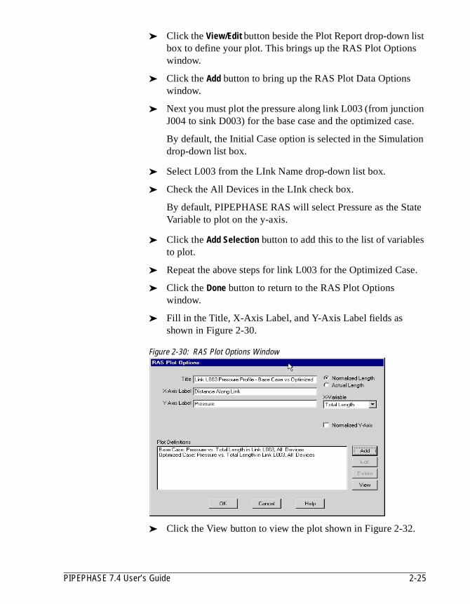
➤ Click the View/Edit button beside the Plot Report drop-down list box to define your plot. This brings up the RAS Plot Options window.
➤ Click the Add button to bring up the RAS Plot Data Options window.
➤ Next you must plot the pressure along link L003 (from junction J004 to sink D003) for the base case and the optimized case.
By default, the Initial Case option is selected in the Simulation drop-down list box.
➤ Select L003 from the LInk Name drop-down list box.
➤ Check the All Devices in the LInk check box.
By default, PIPEPHASE RAS will select Pressure as the State Variable to plot on the y-axis.
➤ Click the Add Selection button to add this to the list of variables to plot.
➤ Repeat the above steps for link L003 for the Optimized Case.
➤ Click the Done button to return to the RAS Plot Options window.
➤ Fill in the Title, X-Axis Label, and Y-Axis Label fields as shown in Figure 2-30.
Figure 2-30: RAS Plot Options Window
➤ Click the View button to view the plot shown in Figure 2-32.
PIPEPHASE 7.4 User’s Guide 2-25
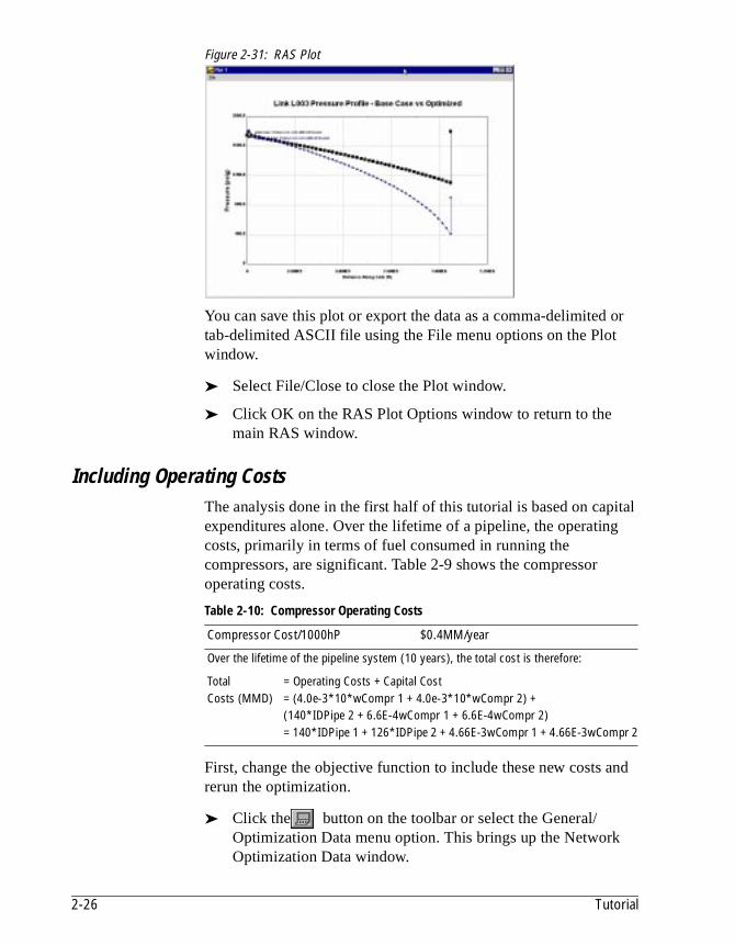
Figure 2-31: RAS Plot
You can save this plot or export the data as a comma-delimited or tab-delimited ASCII file using the File menu options on the Plot window.
➤ Select File/Close to close the Plot window.
➤ Click OK on the RAS Plot Options window to return to the main RAS window.
Including Operating CostsThe analysis done in the first half of this tutorial is based on capital expenditures alone. Over the lifetime of a pipeline, the operating costs, primarily in terms of fuel consumed in running the compressors, are significant. Table 2-9 shows the compressor operating costs.
First, change the objective function to include these new costs and rerun the optimization.
➤ Click the button on the toolbar or select the General/Optimization Data menu option. This brings up the Network Optimization Data window.
Table 2-10: Compressor Operating Costs
Compressor Cost/1000hP $0.4MM/year
Over the lifetime of the pipeline system (10 years), the total cost is therefore:
Total = Operating Costs + Capital CostCosts (MMD) = (4.0e-3*10*wCompr 1 + 4.0e-3*10*wCompr 2) +
(140*IDPipe 2 + 6.6E-4wCompr 1 + 6.6E-4wCompr 2)= 140*IDPipe 1 + 126*IDPipe 2 + 4.66E-3wCompr 1 + 4.66E-3wCompr 2
2-26 Tutorial
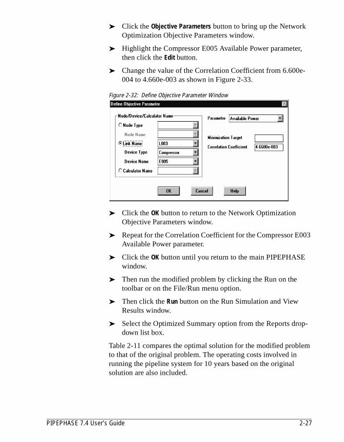
➤ Click the Objective Parameters button to bring up the Network Optimization Objective Parameters window.
➤ Highlight the Compressor E005 Available Power parameter, then click the Edit button.
➤ Change the value of the Correlation Coefficient from 6.600e-004 to 4.660e-003 as shown in Figure 2-33.
Figure 2-32: Define Objective Parameter Window
➤ Click the OK button to return to the Network Optimization Objective Parameters window.
➤ Repeat for the Correlation Coefficient for the Compressor E003 Available Power parameter.
➤ Click the OK button until you return to the main PIPEPHASE window.
➤ Then run the modified problem by clicking the Run on the toolbar or on the File/Run menu option.
➤ Then click the Run button on the Run Simulation and View Results window.
➤ Select the Optimized Summary option from the Reports drop-down list box.
Table 2-11 compares the optimal solution for the modified problem to that of the original problem. The operating costs involved in running the pipeline system for 10 years based on the original solution are also included.
PIPEPHASE 7.4 User’s Guide 2-27
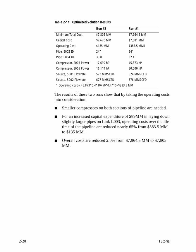
The results of these two runs show that by taking the operating costs into consideration:
■ Smaller compressors on both sections of pipeline are needed.
■ For an increased capital expenditure of $89MM in laying down slightly larger pipes on Link L003, operating costs over the life-time of the pipeline are reduced nearly 65% from $383.5 MM to $135 MM.
■ Overall costs are reduced 2.0% from $7,964.5 MM to $7,805 MM.
Table 2-11: Optimized Solution Results
Run #2 Run #1
Minimum Total Cost $7,805 MM $7,964.5 MM
Capital Cost $7,670 MM $7,581 MM
Operating Cost $135 MM $383.5 MM1
Pipe, E002 ID 24” 24”
Pipe, E004 ID 33.0 32.1
Compressor, E003 Power 17,699 hP 45,873 hP
Compressor, E005 Power 16,114 hP 50,000 hP
Source, S001 Flowrate 573 MMSCFD 524 MMSCFD
Source, S002 Flowrate 627 MMSCFD 676 MMSCFD
1 Operating cost = 45.873*0.4*10+50*0.4*10=$383.5 MM
2-28 Tutorial

IndexA
Additional Component Capabilities 1-16
Additional Thermodynamic Capabilities 1-20
Assay Curve 1-16
D
Defaults 1-12
DefiningFluid Properties 1-13Properties for Compositional Fluids 1-14Properties for Mixed Compositional/ Non-Compositional Fluids 1-23Properties for Non-compositional Fluids
Liquid 1-20
Documentation vi
E
Exiting PIPEPHASE 1-2
G
Gaslift and Sphering 1-10
Generating and Using Tables of Properties 1-24
H
Heat Transfer Calculations 1-40
Help, online vii
L
Library Components 1-14
N
Nodal Analysis 1-49
Nominal Diameter 1-33
Non-library Components 1-15
O
Onlinedocumentation vihelp vii
P
Petroleum Pseudocomponents 1-15
Pipe Schedule 1-33
PIPEPHASECase Studies 1-47Changing Window Size 1-3Color Coding Cues 1-3Equipment Items 1-37Global Settings 1-10Main Window Components 1-2Menu Options 1-4Toolbar Buttons 1-5Units of Measurement 1-11
Piping Structure 1-10
Pressure Drop in Completions 1-35
Pressure Drop in Fittings 1-35
Pressure Drop in Flow Devices 1-32
Printout Options 1-11
Production Planning 1-42
Properties for Non-compositional FluidsLiquid
GasSteam
Gas CondensateBlackoil 1-21
PIPEPHASE 7.4 User’s Guide I-1
R
RelationshipsReservoirs and Inflow Performance 1-41
S
Sources 1-24
Sphering or Pigging 1-41
Starting PIPEPHASE 1-1
Structure of Network Systems 1-25
Subsurface Networks and Multiple Completion Modeling 1-44
T
Technical support centers ix
Thermodynamic Properties and Phase Separation 1-17
Time-stepping 1-42
Transport Properties 1-19
U
Using PIPEPHASE 1-7
V
Viewing and Plotting Results 2-23
Index I-2