pierre-olivier gourinchas, thomas philippon, dimitri
TRANSCRIPT

Pierre-Olivier Gourinchas, Thomas Philippon, Dimitri Vayanos
The analytics of Greek crisis Article (Published version) (Refereed)
Original citation: Gourinchas, Pierre-Olivier and Philippon, Thomas and Vayanos, Dimitri (2017) The analytics of the Greek crisis. NBER Macroeconomics Annual, 31 (1). pp. 1-81. ISSN 0889-3365 DOI: 10.1086/690239 © 2017 by the National Bureau of Economic Research This version available at: http://eprints.lse.ac.uk/82433/ Available in LSE Research Online: June 2017 LSE has developed LSE Research Online so that users may access research output of the School. Copyright © and Moral Rights for the papers on this site are retained by the individual authors and/or other copyright owners. Users may download and/or print one copy of any article(s) in LSE Research Online to facilitate their private study or for non-commercial research. You may not engage in further distribution of the material or use it for any profit-making activities or any commercial gain. You may freely distribute the URL (http://eprints.lse.ac.uk) of the LSE Research Online website.

© 2017 by the National Bureau of Economic Research. All rights reserved.978- 0- 226- 39560- 9/2017/2017- 0101$10.00
1
The Analytics of the Greek Crisis
Pierre- Olivier Gourinchas, UC Berkeley, NBER, and CEPR
Thomas Philippon, NYU Stern and NBER
Dimitri Vayanos, London School of Economics, NBER, and CEPR
Gourinchas, Philippon, and Vayanos
I. Introduction and Motivation
The economic crisis that Greece has been experiencing from 2008 on-ward has been particularly severe. Real gross domestic product (GDP) per capita stood at approximately €22,600 in 2008, and dropped to €17,000 by 2014, a decline of 24.8%.1 The unemployment rate was 7.8% in 2008, and rose to 26.6% in 2014. The entire Greek banking system became insolvent during the crisis, and a large- scale recapitalization took place in 2013. In 2012, Greece became the first Organisation for Economic Co- operation and Development (OECD) member country to default on its sovereign debt, and that default was the largest in world history. Greece received financial assistance from other Eurozone (EZ) countries and the International Monetary Fund (IMF), and the size of this bailout package was also the largest in history.
The implications of the Greek crisis extended well beyond Greece. The bailout package that Greece received was large partly because of fears of contagion to other countries in the EZ and to their banking sys-tems. Moreover, at various stages during the crisis, the continued mem-bership of Greece in the EZ was put in doubt. This tested the strength and the limits of the currency union, and of the European project more generally.
This paper provides an “interim” report on the Greek crisis (“interim” in the sense that the crisis is still unfolding). We proceed in three steps. First, we describe the main macroeconomic dynamics that Greece experi-enced before and during the crisis. Second, we put these dynamics in per-spective by benchmarking the Greek crisis against all episodes of sudden stops, sovereign debt crises, and lending boom/busts in emerging and
This content downloaded from 158.143.197.030 on June 27, 2017 04:08:23 AMAll use subject to University of Chicago Press Terms and Conditions (http://www.journals.uchicago.edu/t-and-c).

2 Gourinchas, Philippon, and Vayanos
advanced economies since 1980. Third, we develop a dynamic stochas-tic general equilibrium (DSGE) model designed to capture many of the relevant features of the Greek crisis and help us identify its main drivers.
The global financial crisis that began in 2007 in the United States hit Greece through three interlinked shocks. The first shock was a sovereign debt crisis: investors began to perceive the debt of the Greek government as unsustainable, and were no longer willing to finance the government deficit. The second shock was a banking crisis: Greek banks had diffi-culty financing themselves in the interbank market, and their solvency was put in doubt because of projected losses to the value of their assets. The third shock was a sudden stop: foreign investors were no longer will-ing to lend to Greece as a whole (government, banks, and firms), and so the country could not finance its current account deficit.
To many observers, that last shock was a startling development. After all, the very existence of a common currency, and therefore of an auto-matic provision of liquidity against good collateral through its common central bank, was supposed to insulate member countries against a sudden reversal of private capital of the kind experienced routinely by emerging- market (EM) economies. Just like a sudden stop on California or Texas could not happen since Federal Reserve funding would substi-tute instantly and automatically for private capital, the common view was a sudden stop could not happen to Greece or Portugal since Euro-pean Central Bank (ECB) funding would substitute instantly and auto-matically for private capital.2 The belief that sudden stops were a thing of the past may have, in turn, contributed to the emergence of mount-ing internal and external imbalances, in Greece and elsewhere in the EZ (Blanchard and Giavazzi 2002). Yet, at the onset of the crisis, Greece and other EZ members did experience a classic sudden stop. The built- in defense mechanisms of the EZ were activated and the ECB provided much needed funding to the Greek economy. How much, then, did this sudden stop contribute to the subsequent meltdown and through what channels? And what was the contribution of other factors? These are among the questions that we seek to address in this paper.
The first main result that emerges from our macro- benchmarking ex-ercise is that Greece’s drop in output (a 25% decline in real GDP per capita between 2008 and 2013) was significantly more severe and pro-tracted than during the average crisis. This applies to the sample of countries that experienced sudden stops, to the sample that experienced sovereign defaults, to the sample that experienced lending booms and busts, and even to the sample that experienced all three shocks com-
This content downloaded from 158.143.197.030 on June 27, 2017 04:08:23 AMAll use subject to University of Chicago Press Terms and Conditions (http://www.journals.uchicago.edu/t-and-c).

The Analytics of the Greek Crisis 3
bined (we call these episodes “trifectas”). The collapse in investment (75% decline between 2008 and 2013) was even more severe. Impor-tantly, we find that the difference in output dynamics is not driven by the exchange- rate regime. Countries whose currency remains pegged experience a larger output drop, on average, than countries with float-ing rates. But unlike these countries, whose output rebounds after a few years, Greece’s output continued to drop to a significantly lower level.
One possible explanation for the severity of Greece’s crisis is the high level of debt—government, private, and external—at the onset of the crisis. Greece’s government debt stood at 103.1% of output in 2007, its net foreign assets at –99.9% of output, and its private- sector debt at 92.4% of output. On the former two measures, Greece fared worse than Ireland, Italy, Portugal, and Spain, the four other major EZ countries hit by the crisis. Greece fared worse than those countries also on its govern-ment deficit and current- account deficit, which stood at 6.5% and 15.9% of output, respectively, in 2007. And debt levels in Greece were more than twice as large than the average of the emerging- market economies, which account for most of the crisis episodes in our sample.
To identify the role of debt, as well as of other factors such as the sudden stop of private capital in driving the severity of the Greek cri-sis, we turn to our DSGE model. The model is designed to capture in a simple and stylized manner the three types of shocks that hit Greece. It also captures a rich set of interdependencies between the shocks. The model features a government, two types of consumers, firms, and banks. The government can borrow, raise taxes, spend, and possibly default on its debt. Consumers differ in their subjective discount rate. Impatient consumers are those who borrow in equilibrium, subject to a debt limit. Firms can borrow and invest and face sticky wages and prices. Consumers and firms can borrow from banks and can default on their debts. The rates at which the government, consumers, and firms can borrow depend on the probability with which these entities can default and on the losses given default. In turn, the expected costs of default (probability times losses) depend on the ratio of debt to income.
In the model, a sovereign risk shock increases the government’s fund-ing costs. The government responds by increasing taxes and reducing expenditures, which exerts a contractionary effect on the economy. In turn, the decline in output increases the expected costs of default on private- sector loans, causing funding costs for consumers and firms to rise and investment to drop. Conversely, a sudden stop increases directly the rate at which consumers and firms can borrow, causing in-
This content downloaded from 158.143.197.030 on June 27, 2017 04:08:23 AMAll use subject to University of Chicago Press Terms and Conditions (http://www.journals.uchicago.edu/t-and-c).

4 Gourinchas, Philippon, and Vayanos
vestment, consumption, and output to decline. The decline in fiscal rev-enues pushes up sovereign yields and has an adverse impact on public debt dynamics. Hence, in our model, sovereign risks and private- sector risks are intertwined and shocks to one sector of the economy can affect funding costs and default rates throughout all sectors.
We estimate the model using Bayesian methods and annual data on government revenue and spending, household debt, nonperforming loans in the private sector, borrowing rates for the government and the corporate sector, as well as price and wage inflation. The model features eight stochastic shocks in each year, identical to the number of variables that we use in the estimation. We find that the model does an excel-lent job of matching additional variables such as output, investment, and the current account (which the model was not asked to replicate). We then perform two tasks with the model. First, we decompose the movements in output, investment, and other key variables into the con-tribution of each type of shock. This helps us determine which shocks were the most important in driving the crisis dynamics. Second, we use the model to perform a number of “counterfactuals” to identify the role played by different aspects of the institutional environment. We examine, in particular, how the dynamics of output and investment would have been different if debt levels in Greece were set at the av-erage of emerging- market economies, if banks’ funding costs had not increased during the crisis as a possible effect of a European banking union, if the Greek government had followed a more virtuous fiscal path in the years preceding the crisis, and if prices and wages had been more flexible.
As in Agatha Christie’s Murder on the Orient Express, our model indi-cates that many forces contributed to the “murder” of the Greek econ-omy. Yet a few factors stand out. First and most importantly, given the size of the fiscal imbalances, a substantial fiscal correction was inevi-table. According to our estimates, fiscal consolidation accounted for ap-proximately 50% of the output drop from peak to trough. Much of the remainder is explained by the increase in funding costs for the private sector (“sudden stop” in our model) and the sovereign (“sovereign risk shock”). The combination of the two shocks accounted for an additional 40% of the output drop from peak to trough, with the sudden stop driv-ing more than half of the effect.
Lastly, our estimates indicate that markup shocks in product mar-kets and a surge in nonperforming loans contributed significantly to the lack of recovery in 2014 and 2015: in the absence of these shocks,
This content downloaded from 158.143.197.030 on June 27, 2017 04:08:23 AMAll use subject to University of Chicago Press Terms and Conditions (http://www.journals.uchicago.edu/t-and-c).

The Analytics of the Greek Crisis 5
output in 2014–15 would have recovered approximately 35% of its peak- to- trough drop. These findings indicate that the external dimen-sion of the crisis may slowly be fading, and that the forces holding back the Greek economy are now largely domestic and microeconomic: the recovery will entail cleaning up nonperforming loans and facili-tating the adjustment of prices relative to wages. The lack of a suffi-cient price adjustment may have been due to limited competition in goods and services markets, as well as to a rise in firms’ costs stemming from factors such as the uncertainty about EZ exit and the taxation of key inputs.
The effects of the shocks described above were made larger by high leverage and low price flexibility. Our counterfactual exercises allow us to examine more directly the effects of these factors. We find that if the levels of government, private, and external debt in Greece had been comparable to those in the average of the emerging- market economies (so smaller by about half), the peak- to- trough decline in output would have been smaller by about a third, and the same conclusion holds if the prices and wages had been twice as flexible.
II. The Greek Economy before and during the Crisis
This section describes the dynamics of key macroeconomic variables in Greece before and during the crisis. We focus on the behavior of output and investment, as well as on the accumulation of debt—government, private, and external. We also describe the three shocks through which the global financial crisis affected Greece (sudden stop, sovereign debt crisis, and banking crisis) as well as their interrelationships. This sets the stage for the empirical exercise in section III, and motivates some of the modeling choices and analysis in sections IV–VI.
A. Pre- crisis
Output
Figure 1 plots GDP per capita in 2014 US dollars, adjusted for purchas-ing power parity (PPP) and in a log scale from 1980 onward. In this figure, as well as in subsequent figures and tables in this section, we compare Greece to the four other major Eurozone (EZ) countries that were hit by the EZ crisis: Ireland (IE), Italy (IT), Spain (ES), and Por-tugal (PT).
This content downloaded from 158.143.197.030 on June 27, 2017 04:08:23 AMAll use subject to University of Chicago Press Terms and Conditions (http://www.journals.uchicago.edu/t-and-c).

6 Gourinchas, Philippon, and Vayanos
As of 1980, Greek GDP per capita was above that of Ireland, Por-tugal, and Spain. During the 1980s, Greece experienced relative stag-nation and was overtaken by Ireland and Spain. Greece grew faster during the period 1996–2000 and especially from 2001, when it entered the Eurozone (EZ), until 2008. By 2008, Greece had almost caught up with Spain.
Motivated by figure 1, we divide the period 1996–2014 into three subperiods: the period 1996–2000, during which Greece experienced a boom in anticipation of EZ entry; the period 2001–2008, during which the boom continued with Greece inside the EZ; and the crisis period 2009–2014. In the tables constructed in the rest of this section, we report averages of macroeconomic variables for the three subperiods. In some of the tables we also compare with the year 1995, which we take as in-dicative of the Greek economy before the (actual or anticipated) effects of EZ entry.3
Investment
Table 1 reports the level of investment in Greece during the periods 1996–2000, 2001–2008, and 2009–2014, and compares with 1995. The table also decomposes investment into corporate, residential, and public and compares with Ireland, Italy, Portugal, and Spain. Greece experienced the second- largest increase in corporate investment from
Fig. 1. GDP per capita for Greece and other EZ crisis countries, 1980–2014Source: The data come from the Conference Board Total Economy Database. The GDP is expressed in 2014 US dollars, is adjusted for PPP using 2011 weights, and is plotted in a log scale.
This content downloaded from 158.143.197.030 on June 27, 2017 04:08:23 AMAll use subject to University of Chicago Press Terms and Conditions (http://www.journals.uchicago.edu/t-and-c).

Tab
le 1
Inve
stm
ent i
n G
reec
e an
d o
ther
EZ
Cri
sis
Cou
ntri
es, 1
995–
2014
, as
Perc
enta
ge o
f GD
P
Tota
l Inv
estm
ent
95
96–0
0
01–0
8
09–1
4
ES
22.0
23.7
28.8
21.0
GR
20.4
23.1
23.7
14.6
IE18
.222
.326
.116
.2IT
19.0
19.4
21.1
18.6
PT
23.3
26
.5
23.9
17
.4
Cor
pora
te In
vest
men
tR
esid
enti
al In
vest
men
tPu
blic
Inve
stm
ent
95
96–0
0
01–0
8
09–1
4
95
96–0
0
01–0
8
09–1
4
95
96–0
0
01–0
8
09–1
4
ES
11.7
13.0
13.9
12.0
6.0
7.0
10.7
5.7
4.3
3.7
4.2
3.3
GR
8.4
10.5
10.3
7.7
8.6
8.8
9.2
3.7
3.4
3.8
4.2
3.2
IE10
.612
.311
.411
.05.
27.
110
.62.
72.
42.
94.
12.
5IT
11.3
11.8
12.9
10.8
5.1
4.8
5.3
5.1
2.6
2.8
2.9
2.7
PT
11.6
13
.8
13.7
11
.1
7.3
7.
7
6.1
3.
1
4.4
5.
0
4.1
3.
2
Sour
ce: T
he d
ata
com
e fr
om A
ME
CO
. Inv
estm
ent
is m
easu
red
by
the
seri
es “
gros
s fix
ed c
apit
al f
orm
atio
n: t
otal
eco
nom
y,”
and
doe
s no
t in
clud
e in
vent
orie
s. R
esid
enti
al in
vest
men
t is
mea
sure
d b
y “g
ross
fixe
d c
apit
al fo
rmat
ion:
dw
ellin
gs”;
cor
pora
te in
vest
men
t by
“gro
ss fi
xed
cap
ital
form
a-ti
on: p
riva
te s
ecto
r” m
inus
res
iden
tial
inve
stm
ent;
and
pub
lic in
vest
men
t by
“gro
ss fi
xed
cap
ital
form
atio
n: g
over
nmen
t.”
This content downloaded from 158.143.197.030 on June 27, 2017 04:08:23 AMAll use subject to University of Chicago Press Terms and Conditions (http://www.journals.uchicago.edu/t-and-c).

8 Gourinchas, Philippon, and Vayanos
Fig. 2. Net foreign assets in Greece and other EZ crisis countries, 1980–2014, as per-centage of GDP.Source: The data come from Lane and Milesi- Ferretti (2007).
1995 to 1996- 2000, after Portugal. Corporate investment remained at that elevated level during 2001- 2008. Thus, EZ entry and its anticipation was associated with a significant rise in corporate investment in Greece. That rise, however, occurred from a low base, and corporate investment remained significantly lower than in the other countries.
Unlike Ireland and Spain, Greece did not experience a significant increase in residential investment from 1995 to 1996–2008. Residential investment was already high in 1995, however, and the real estate boom in Ireland and Spain only meant that residential investment in those countries caught up with and exceeded somewhat that in Greece.
Net Foreign Assets
The fast growth of Greek GDP per capita during the period 1996–2008 was associated with an increase in external indebtedness. Figure 2 plots net foreign assets (NFA) from 1980 onward as percentage of GDP. The NFA for Greece were negative throughout that period. They were a relatively small fraction of GDP in absolute value until the mid- 1990s, and they subsequently declined to a much more negative fraction. Greece’s NFA position deteriorated at a comparable rate to Portugal’s and Spain’s, while Ireland experienced a more abrupt deterioration. The behavior of Greece’s NFA from the mid- 1990s onward is indicative of large current account deficits. Table 2 reports the level of the current
This content downloaded from 158.143.197.030 on June 27, 2017 04:08:23 AMAll use subject to University of Chicago Press Terms and Conditions (http://www.journals.uchicago.edu/t-and-c).

Tab
le 2
The
Cur
rent
Acc
ount
in G
reec
e an
d o
ther
EZ
Cri
sis
Cou
ntri
es, 1
995–
2014
, as
Perc
enta
ge o
f GD
P
Cur
rent
Acc
ount
Sur
plus
Net
Exp
orts
Net
Cur
rent
Tra
nsfe
rs P
lus
Net
Pri
mar
y In
com
es
95
96–0
0
01–0
8
09–1
4
95
96–0
0
01–0
8
09–1
4
95
96–0
0
01–0
8
09–1
4
ES
–1.2
–2.0
–6.7
–1.6
–1.0
–1.1
–4.1
0.8
–0.2
–0.9
–2.6
–2.4
GR
–2.8
–5.7
–11.
7–7
.3–8
.3–9
.1–1
0.6
–5.9
5.5
3.4
–1.1
–1.4
IE2.
61.
2–2
.31.
710
.912
.012
.419
.2–8
.3–1
0.8
–14.
7–1
7.5
IT2.
01.
5–1
.1–1
.03.
72.
80.
10.
4–1
.7–1
.3–1
.2–1
.4PT
–3
.4
–7.7
–9
.8
–4.5
–6
.4
–9.1
–8
.5
–3.0
3.
0
1.4
–1
.3
–1.5
Sour
ce: T
he d
ata
com
e fr
om A
ME
CO
. Net
exp
orts
are
mea
sure
d b
y th
e se
ries
“ne
t exp
orts
of g
ood
s an
d s
ervi
ces”
; net
cur
rent
tran
sfer
s by
“ne
t cur
-re
nt tr
ansf
ers
from
the
rest
of t
he w
orld
”; a
nd n
et p
rim
ary
inco
me
by “
net p
rim
ary
inco
me
from
the
rest
of t
he w
orld
.” T
he c
urre
nt a
ccou
nt s
urpl
us
is th
e su
m o
f the
thre
e se
ries
.
This content downloaded from 158.143.197.030 on June 27, 2017 04:08:23 AMAll use subject to University of Chicago Press Terms and Conditions (http://www.journals.uchicago.edu/t-and-c).

10 Gourinchas, Philippon, and Vayanos
account in Greece, Ireland, Italy, Portugal, and Spain during the periods 1996–2000, 2001–2008, and 2009–2014, and compares with 1995. The table decomposes the current account into (a) net exports and (b) the sum of net current transfers and net primary income.
Greece’s current account deteriorated from 1995 to 1996–2000, and deteriorated further from 2001 to 2008. The deterioration from 1996–2000 to 2001–2008 was particularly severe: 6.0% of GDP, larger than in the other countries. From 2001 to 2008, Greece was running an average current account deficit of 11.7% of GDP, also larger than in the other countries.
The deterioration of Greece’s current account from 1995 onward was primarily driven by a decline in net current transfers and net primary income. Net current transfers to Greece declined partly because of the drop in EU subsidies, especially after the 2005 EU enlargement, as funds were redirected to new entrants that were poorer than Greece. Net primary income also declined because workers’ remittances be-came smaller as Greece became a net immigration country and because of growing interest payments on Greece’s rising external debt. Greece’s trade balance also deteriorated through that period, reaching –10.6% of GDP during the period 2001–2008.
The increase in Greece’s current account deficit from 1995 to 1996–2000 was associated with an increase in corporate investment and, hence, in productive capacity. Indeed, the current account deficit in-creased by 2.9% of GDP, corporate investment increased by 2.1%, and public investment by 0.4%. The increase in the current account deficit from 1996–2000 to 2001–2008, however, was associated with an increase in consumption. Indeed, the current account deficit increased by 6.0% of GDP, total saving declined by 6.7%, and corporate investment dropped slightly. The decline in total saving from 1996–2000 to 2001–2008 was primarily driven by private saving, which declined by 4.3% of GDP.4
Government Debt
Figure 3 plots government debt from 1980 onward, as percentage of GDP. As of 1980, government debt in Greece was 21.4% of GDP, lower than in all other countries except for Spain. Debt rose sharply during the 1980s, and by 1993 it had reached 94.4% of GDP, a level larger than in all other countries except for Italy. A combination of fiscal tighten-ing to meet the criteria for EZ entry, and sharply lower interest rates in anticipation of that entry, helped stabilize and even reduce slightly
This content downloaded from 158.143.197.030 on June 27, 2017 04:08:23 AMAll use subject to University of Chicago Press Terms and Conditions (http://www.journals.uchicago.edu/t-and-c).

The Analytics of the Greek Crisis 11
the ratio of debt to GDP to 88.5% in 1999. Budget discipline became looser after EZ entry, and especially after 2007. As a consequence, debt to GDP increased—to 103.1% in 2007 and 126.8% in 2009—despite the fast growth in GDP during the period 2001–2008.
While debt to GDP increased only mildly from 1999 to 2007, there was a sharp increase in the amount of the debt held by foreign entities and a consequent decrease in the amount held domestically. That trend was due mainly to the decline in private saving. Figure 4 plots gross government external debt for Greece, and compares with the same se-
Fig. 4. Gross government external debt for Greece, Portugal, and Spain, 1999–2013, as percentage of GDP.Source: The data come from the ECB, series “gross external debt: government.” The data are quarterly, and we report the average over each year.
Fig. 3. Government debt in Greece and other EZ crisis countries, 1980–2014, as per-centage of GDP.Source: The data come from AMECO, series “general government consolidated gross debt.”
This content downloaded from 158.143.197.030 on June 27, 2017 04:08:23 AMAll use subject to University of Chicago Press Terms and Conditions (http://www.journals.uchicago.edu/t-and-c).

12 Gourinchas, Philippon, and Vayanos
ries for Portugal and Spain, and with Greece’s NFA.5 Gross government external debt for Greece essentially coincides with the negative of NFA. By contrast, gross government external debt for Portugal and Spain is significantly lower than the negative of those countries’ NFA (which are not plotted, but are similar to Greece’s from figure 2). Figure 4 thus indicates that Greece’s current account deficit essentially financed gov-ernment borrowing.6
Figure 5 plots government deficit as percentage of GDP. The figure com-pares Greece to Italy, which was the most similar to Greece in terms of the size of its government debt until the crisis, and to the EU average. The figure shows that Greece’s public finances improved in the run- up to EZ entry, but worsened steadily post- entry. The pre- entry improvement was similar to that in Italy and the EU average. Unlike in Greece, however, the latter series remained relatively stable post- entry and until the crisis.
Banks and Credit
From the mid- 1990s until the crisis, Greece experienced a boom in private credit. An extensive program of financial liberalization that took
Fig. 5. Government deficit in Greece, Italy, and the EU average, 1985–2014, as percent-age of GDP.Source: The data come from the EC, series “surplus (net lending or net borrowing: general government).”
This content downloaded from 158.143.197.030 on June 27, 2017 04:08:23 AMAll use subject to University of Chicago Press Terms and Conditions (http://www.journals.uchicago.edu/t-and-c).

The Analytics of the Greek Crisis 13
place in the late 1980s and the 1990s paved the way for the credit boom. It was also fueled by easier access to foreign capital following EZ entry (and the anticipation of it). Figure 6 plots bank loans to the nonfinancial private sector for Greece, Ireland, Italy, Portugal, and Spain, as percent-age of GDP.
Private- sector loans to GDP were significantly lower in Greece than in the other countries before EZ entry: they stood at 34.1% of GDP in 1998, compared to 60.8% in Italy, 74.6% in Spain, 80.31% in Portugal, and 82.8% in Ireland. Loans to GDP grew faster in Greece than in any other country, however, after EZ entry. As of 2008, they stood at 103.0%, a ratio smaller than Ireland’s, Portugal’s, and Spain’s, but larger than Italy’s.
To finance their increasing lending activity, Greek banks became more reliant on wholesale funding through the interbank market. Figure 7 plots gross external debt for Greek banks and compares with Italy, Por-tugal, and Spain. Gross external debt of banks consists mainly of inter-bank loans. Gross external debt of Greek banks increased from 12.3% of GDP in 1999 to 46.2% of GDP in 2008. As in the case of private- sector loans to GDP, the growth rate was higher than in the other countries, and the 2008 level was smaller than Portugal’s and Spain’s, but larger than Italy’s.
Fig. 6. Bank loans to the private sector excluding financial firms in Greece and other EZ crisis countries, 1998–2014, as percentage of GDP.Source: The loans data come from the Bank of Greece (BoG) in the case of Greece and from the European Central Bank (ECB) for the other countries. The loan data are monthly and are sampled in December of each year.
This content downloaded from 158.143.197.030 on June 27, 2017 04:08:23 AMAll use subject to University of Chicago Press Terms and Conditions (http://www.journals.uchicago.edu/t-and-c).

14 Gourinchas, Philippon, and Vayanos
B. Crisis
The Three Shocks
The global financial crisis that began in 2007 found Greece in a highly vulnerable position. As of 2007, Greece’s current account deficit had reached 15.9% of GDP, NFA stood at –99.9%, government deficit at 6.5%, and government debt at 103.1%. On all four measures, Greece fared worse than Ireland, Italy, Portugal, and Spain. Greece’s bank-ing system was also vulnerable. While the ratio of private- sector loans to GDP in Greece was lower than in Ireland, Portugal, and Spain, the exposure of Greek banks to their sovereign was larger than in those countries.
Greece was hit by three interdependent shocks during the crisis. The first shock was a sovereign debt crisis: investors began to perceive the debt of the Greek government as unsustainable, and were no longer willing to finance the government deficit. The second shock was a bank-ing crisis: Greek banks had difficulty financing themselves, and their solvency was put in doubt because of projected losses to the value of their assets. The third shock was a sudden stop: foreign investors were no longer willing to lend to Greece as a whole (government, banks, and
Fig. 7. Gross external debt of financial firms for Greece and other EZ crisis countries, 1999–2013, as percentage of GDP.Source: The data come from the ECB, series “Gross External Debt: MFIs.” The data are quarterly and we report the average over each year. We exclude the series for Ireland, which rises up to 425% of GDP, so that the series for the other countries can be seen more clearly.
This content downloaded from 158.143.197.030 on June 27, 2017 04:08:23 AMAll use subject to University of Chicago Press Terms and Conditions (http://www.journals.uchicago.edu/t-and-c).

The Analytics of the Greek Crisis 15
firms), and so the country could not finance its current account deficit, nor roll over its maturing gross liabilities.
The three shocks were interlinked. The banking crisis made the gov-ernment’s fiscal problems worse. This was because the government had to inject equity capital into the banks and had to provide them with guarantees so that they could borrow in the interbank market. Moreover, because banks had to curtail their lending, the economy slowed down and the government’s tax revenues declined. These channels were at play starting from the fall of 2008, when Greek banks faced significant difficulties financing themselves in the interbank market. The Greek government passed a law in December 2008 that provided support to the banks in the form of guarantees and equity capital.
Conversely, the sovereign crisis made the banks’ liquidity and solvency problems worse. This was because concerns about default risk by the Greek government reduced the value of the Greek banks’ government- bond portfolio, and this put the banks’ solvency in doubt. Moreover, the government had to engage in significant fiscal tightening, and the ensuing recession meant that firms and house-holds had difficulty repaying their loans, adding to the banks’ sol-vency problems. Finally, the guarantees given by the government to Greek banks diminished in value. That applied both to the guarantees intended to help the banks borrow in the interbank market and to the government- supplied deposit insurance. Hence, banks had more dif-ficulties financing themselves and their liquidity problems worsened. These channels were at play beginning in September 2009, when in-vestors began to perceive the debt of the Greek government as unsus-tainable.
Both the sovereign and the banking crises were closely linked to the sudden stop. Indeed, most of government debt was held by foreign investors: out of government debt equal to 103.1% of GDP in 2007, the debt held by foreign investors was 76.1% of GDP. Greek financial firms also had significant foreign debt: their gross external debt was 41.8% of GDP in 2007. Since the Greek government and Greek banks intermedi-ated most of the flow of foreign capital to Greece, the withdrawal of foreign capital meant that both sectors’ access to funds was seriously impaired.
Ireland, Italy, Portugal, and Spain were hit by some or all of the same shocks. The shocks’ effects were more severe in the case of Greece, how-ever, given the country’s larger vulnerability.7
This content downloaded from 158.143.197.030 on June 27, 2017 04:08:23 AMAll use subject to University of Chicago Press Terms and Conditions (http://www.journals.uchicago.edu/t-and-c).

16 Gourinchas, Philippon, and Vayanos
Assistance to the Sovereign and Sovereign Default
In May 2010, Greece agreed to follow an adjustment program financed and monitored by European institutions and the IMF. Under the terms of the agreement, Greece received a loan so as to avoid a default on its private creditors and reduce its government deficit more smoothly. In exchange, it had to engage in significant fiscal tightening and imple-ment a battery of structural reforms. The agreed loan amount was 110 billion euros, or 44% of Greece’s 2010 GDP. Out of that amount 80 bil-lion came from other EZ countries, and the remaining 30 billion from the IMF. The first adjustment program was rolled over into a second, agreed to in February 2012. A third program began in August 2015.
In March 2012, Greece agreed to a debt restructuring with its private creditors. Under the terms of this private- sector involvement (PSI), pri-vately held government debt with face value of 199.2 billion euros was replaced by debt with a face value of 92.1 billion. Greece was the only EZ country to default on its creditors.
Assistance to the Banks, Recapitalizations, and Capital Controls
In addition to the loans made to the Greek government under the adjust-ment programs, assistance was provided to Greece through ECB loans to its banking system. These loans were administered either directly from the ECB, with a low interest rate and stringent collateral requirements, or indirectly via the Bank of Greece (BoG) as emergency liquidity assistance (ELA), with a higher interest rate and less stringent collateral requirements. The ECB loans were necessary to address the liquidity problems of Greek banks. They rose from 48 billion euros in January 2010 to a maximum of 158 billion euros in February 2012, then dropped to a minimum of 45 bil-lion euros in November 2014, and then rose again to a maximum of 122 bil-lion in September 2015. The ECB loans were at their maxima around times when there was a high- perceived risk of Greece exiting the EZ (Grexit). The risk of Grexit was high around the double election of May and June 2012, and during the first half of 2015 after a new Greek government op-posed to the adjustment programs had been elected in January 2015.
Greek banks went through a series of recapitalizations. Losses on the banks’ government- bond portfolio reduced the capital of all banks and rendered most of the large ones insolvent. Some of the banks were re-solved, and their deposits and some of the loans were transferred to the four largest banks. The latter were recapitalized. The resolution and re-
This content downloaded from 158.143.197.030 on June 27, 2017 04:08:23 AMAll use subject to University of Chicago Press Terms and Conditions (http://www.journals.uchicago.edu/t-and-c).

The Analytics of the Greek Crisis 17
capitalization process was completed in July 2013, and involved 38.9 bil-lion euros of public funds, which were loaned to Greece. An additional 3.1 billion euros were raised by private investors. That first, large- scale recapitalization was followed by a second in April and May 2014, when the banks raised 8.3 billion euros, solely from private investors. A third recapitalization took place in the fourth quarter of 2015. The total amount that was raised then was 13.7 billion euros, of which 8 billion euros was raised from private sources via new investment and debt- equity conver-sions. The second and third recapitalizations were made necessary be-cause of increased projected losses on banks’ loans to the private sector.
Macroeconomic Developments
We finally review the macroeconomic developments during the crisis period 2009–2014, following a roughly similar order as for the pre- crisis period. Greek GDP per capita declined sharply during the crisis, as shown in figure 1. The decline was 25.8% between 2008 and 2014. It was much sharper than in Ireland (6.1%), Italy (10.3%), Portugal (7.8%), and Spain (9.6%).
The decline in GDP was accompanied by a large decline in invest-ment. The latter decline can be seen in table 1 by comparing the crisis period with the pre- crisis one. It can be seen more sharply by compar-ing investment in 2014 to that in 2008. Investment in 2014 was less than half of its 2008 value, having dropped by 12.2% of GDP. Both the rela-tive and the absolute declines were larger than in Ireland, Italy, Portu-gal, and Spain. The level of investment in 2014 was also significantly lower than in the other countries.
During the crisis, Greece reduced and almost eliminated its current account deficit. That deficit stood at 2.2% of GDP in 2014, down from 16.5% in 2008. The adjustment occurred entirely through a drop in in-vestment. Total saving did not change: government saving increased as a result of the fiscal tightening that took place during the crisis, but that effect was offset by a decline in private saving. Private saving in Greece declined between 2008 and 2014, while it increased in Ireland, Italy, Portugal, and Spain. Conversely, government saving increased in Greece during the same period, while it declined in the other countries. Thus, the austerity undergone by Greece during the crisis was more severe than in the other countries.
During the crisis, public debt to GDP followed explosive dynamics, rising from 103.1% in 2007 and 126.8% in 2009 to 177.1% in 2014. The in-
This content downloaded from 158.143.197.030 on June 27, 2017 04:08:23 AMAll use subject to University of Chicago Press Terms and Conditions (http://www.journals.uchicago.edu/t-and-c).

18 Gourinchas, Philippon, and Vayanos
crease resulted from the deficits run during the crisis and from the drop in GDP. The debt restructuring agreed to in 2012 countered these effects somewhat.8 Greece eliminated its primary budget deficit in 2014—it ran a primary surplus of 0.4% in that year.
The ratio of private- sector loans to GDP declined slowly during the crisis. As figure 6 shows, it stood at almost the same level as Portugal’s and Spain’s in 2014, and above Ireland’s and Italy’s. The slow decline of private- sector loans to GDP in Greece is due to the sharp decline in GDP and the relatively slow pace of resolving nonperforming loans.
III. Benchmarking the Greek Crisis
The previous section argued that Greece experienced three quasi- simultaneous and interlinked shocks: a sudden stop, with the abrupt withdrawal of private foreign capital starting in 2009; a sovereign debt crisis, with rapidly deteriorating fiscal accounts in 2008 and 2009, culminating in a sovereign default in 2012; and a banking crisis with the bursting of a boom in credit to the private nonfinancial sector in 2008 and 2009. This section provides a systematic comparison between Greece and other countries experiencing each type (and sometimes combinations) of similar shocks.
A. The Incidence of Crisis
We begin by identifying episodes of sudden stops, sovereign defaults, and lending booms/busts.
Sudden Stops
Starting with the work of Dornbusch and Werner (1994), Calvo et al. (2006), Adalet and Eichengreen (2007), and many others, an abundant literature has explored the macroeconomic consequences of a sudden reversal in foreign lending. Calvo et al. (2006), in particular, compiled a list of 33 sudden stop episodes between 1980 and 2004 for a sample of 31 emerging markets. In the authors’ classification, a sudden stop is identified by the combination of (a) a reversal in capital flows; (b) an increase in emerging- market bond spreads, capturing times of global stress on financial markets; and (c) a large drop in domestic output. Mendoza (2010) adopts a similar classification, while Korinek and Men-doza (2014) extend the Calvo et al. (2006) sample to 2012 and to ad-
This content downloaded from 158.143.197.030 on June 27, 2017 04:08:23 AMAll use subject to University of Chicago Press Terms and Conditions (http://www.journals.uchicago.edu/t-and-c).

The Analytics of the Greek Crisis 19
vanced economies.9 As in these earlier papers, we define the year t of a sudden stop episode as the year of a sharp reduction in foreign lending that coincides with a large decline in output.10 With this criterion, we identify 49 sudden stop events, 36 for emerging- market economies, and 13 for advanced economies (see table 3).
Sovereign Defaults
We identify sovereign debt crisis as in Gourinchas and Obstfeld (2012). The year t of a sovereign debt crisis corresponds to the year identified with a default on domestic or external public debt, as tabulated by Re-inhart and Rogoff (2009), Cantor and Packer (1995), Chambers (2011), Moody’s (2009) and Sturzenegger and Zettelmeyer (2007).11 Since 1980, we record 64 default episodes in emerging- market economies, and one in an advanced economy: Greece in 2012.
Lending Booms/Busts
Credit boom episodes are defined as in Gourinchas, Valdés, and Landerretche (2001), from the deviation of the ratio of credit to the nonfinancial sector to output from its trend.12 A lending boom episode is recorded when this cyclical deviation exceeds a given boom thresh-old. The year t of the lending boom then coincides with the year in which the maximum (positive) deviation of credit to GDP occurs. Our calculations identify 114 lending boom episodes, 96 of which are in emerging- market economies.
Finally, we identify “trifecta” episodes: sovereign defaults that coincide with a lending boom and a sudden stop.13 We find nine such crises for emerging markets, including well- known episodes such as Mexico in 1982, Chile and Uruguay in 1983, Indonesia and Russia in 1998, Ecua-dor in 1999, Argentina and Turkey in 2001, and Uruguay again in 2003. Again, Greece is the only advanced economy to have experienced a trifecta crisis in our sample.
Table 3 reports the incidence of each type of crisis for advanced and emerging- market economies. It illustrates the relative prevalence of sovereign defaults, lending booms, and trifecta crises among emerging economies. By contrast, sudden stops are roughly distributed in pro-portion to the number of countries in each group in our sample.
We compare each type of episode to the Greek crisis. For the purpose of this exercise, we consider that the Greek episode begins in 2010.14
This content downloaded from 158.143.197.030 on June 27, 2017 04:08:23 AMAll use subject to University of Chicago Press Terms and Conditions (http://www.journals.uchicago.edu/t-and-c).

20 Gourinchas, Philippon, and Vayanos
B. The Data
We construct a database of macrovariables for a large sample of ad-vanced and emerging economies between 1980 and 2014.15 The sample contains 22 advanced economies (including Greece) and 57 emerging- market economies, distributed across six broad regions. The list of emerging- market economies includes all countries classified as emerg-ing according to leading outlets and are therefore reasonably well inte-grated into global bond markets.16
In the spirit of a large literature in international macroeconomics, we examine the behavior of key macroeconomic variables around the three types of shocks discussed above: sudden stops, sovereign debt crises, and lending boom/busts episodes, as well as trifecta crises.17 Our event study considers the response of seven macroeconomic variables: out-put, consumption, investment, exports and imports of goods and ser-vices, the current account, credit to the nonfinancial sector, and public debt. The data is collected from the World Bank’s Development Indica-tors, the IMF’s International Financial Statistics, and Reinhart and Rog-off (2009) estimates of total (domestic and external) gross public debt for a large number of countries.18 In addition to these macroeconomic variables, we use the Reinhart and Rogoff (2004) and Ilzetzki, Reinhart, and Rogoff (2010) de facto exchange rate regime classification and sort countries into “pegs” or “floats” based on the exchange rate regime in the year preceding the episode. Further, we split pegs into “de- peggers,” that is, countries that abandon their peg within two years of the shock, and “strict peggers” who maintain their peg for at least two years. This will allow us to contrast the macroeconomic response of countries based on their post- shock exchange rate regime. This is an important consideration given the often- heard argument that the main constraint on the Greek economy is its lack of nominal exchange rate flexibility (e.g., see Krugman 2012).
Table 3Crises Incidence in Advanced and Emerging Economies, 1980–2014
Sudden
Stop Sovereign
Default Lending
Boom Trifecta No.
Countries
Advanced economies 13 1 18 1 22Emerging markets 36 64 96 9 57Total 49 65 114 10 79
Note: Details on how each type of episode is identified are in the appendix.
This content downloaded from 158.143.197.030 on June 27, 2017 04:08:23 AMAll use subject to University of Chicago Press Terms and Conditions (http://www.journals.uchicago.edu/t-and-c).

The Analytics of the Greek Crisis 21
C. Findings
Figure 8 reports the output response to a typical sudden stop across the 48 episodes (excluding Greece). It measures output per capita, relative to its pre- crisis level at t – 2, in 100 log points, so that a value of x indicates that output per capita is ex/100 times pre- crisis output. The figure also includes point- wise, one- sided 10% confidence intervals (the grayed area), as well as the trajectory of Greek output (bullet points) during the 2010 episode. As expected, since our definition of sudden stops requires a large output drop, the mean response indicates a sharp decline in output, marginally signifi-cant, close to 10% below its peak in the year of the sudden stop, followed by a gradual recovery. By year t + 2, output has typically recovered to its pre- crisis level and continues to expand. Two facts are relevant here. First, Greece experienced a strikingly worse output decline. By 2013, that is, t + 3, Greek output per capita was 25% below its pre- crisis level (e–0.29 = 0.75), significantly below the average response and showing few signs of re-covery. Second, unlike the typical sudden stop, Greece’s output path was “back loaded.” The initial recession in 2009 and 2010 (t – 1 and t) is similar to a typical sudden stop episode and milder than the subsequent
Fig. 8. The response of output to a sudden stopSource: See the appendix for data sources.Note: The figure reports real output per capita relative to period t – 2, in 100 log points for a typical sudden stop episode (with output collapse) and for Greece in the 2010 crisis.
This content downloaded from 158.143.197.030 on June 27, 2017 04:08:23 AMAll use subject to University of Chicago Press Terms and Conditions (http://www.journals.uchicago.edu/t-and-c).

22 Gourinchas, Philippon, and Vayanos
decline in Greek output. By contrast, typical episodes are “front loaded” with a more pronounced “V” shape.19 This is not surprising if we con-sider that Greece’s sudden stop was of a particular nature. As discussed in the previous section, the sudden withdrawal of foreign lending was accommodated initially via ECB lending against collateral, and after 2010 via official assistance from the IMF and the European Union. Hence there was no sharp immediate downturn, as is typical when countries experi-ence sudden loss of market access.
Claim 1. The Greek crisis was significantly more severe, persistent, and back loaded than the typical sudden stop.
Figure 9 reports a similar analysis for the consumption and invest-ment ratios to output. As for output, each variable is expressed in 100 log points, relative to its value at t – 2, that is, at the beginning of the episode. Equivalently, this figure reports the growth differential be-tween consumption or investment and output since t – 2. The top panel reports the consumption- to- output ratio. In a typical sudden stop, con-sumption mostly moves in line with output. Instead, Greek consump-tion grew modestly faster than output, although not significantly so. The bottom panel reports the investment- to- output ratio. Greek invest-ment collapsed dramatically, much more so than in a typical sudden stop. By 2013, that is, t + 3, the investment- to- output ratio was less than half of its pre- crisis level (e–0.76 = 0.47), while a typical sudden stop sees a decline of 20% to 30%. Given the decline in output per capita docu-mented in figure 8, real investment per capita collapsed by almost two- thirds between 2008 and 2013 (0.75 × 0.47 = 0.35).
Claim 2. The collapse in Greek aggregate investment in this crisis was unprece-dented in its persistence and magnitude, in comparison to the typical sudden stop.
A sudden withdrawal of foreign capital is only one of the shocks that Greece experienced since 2009, and one might be concerned that the previous comparison might be too unfavorable to Greece. For instance, like Greece in 2010, Argentina in 2001, Chile in 1983, or Indonesia in 1998, among others, experienced a simultaneous drying- up of foreign capital, a sovereign default, and a collapse in lending, that is, a trifecta shock. These episodes are among the worst documented economic crises in postwar history, often accompanied by a banking crisis, and unprecedented levels of economic hardship and political turmoil. In light of the economic and political dislocation associated with it, one would expect the Greek crisis to be on a comparable scale. To investi-
This content downloaded from 158.143.197.030 on June 27, 2017 04:08:23 AMAll use subject to University of Chicago Press Terms and Conditions (http://www.journals.uchicago.edu/t-and-c).
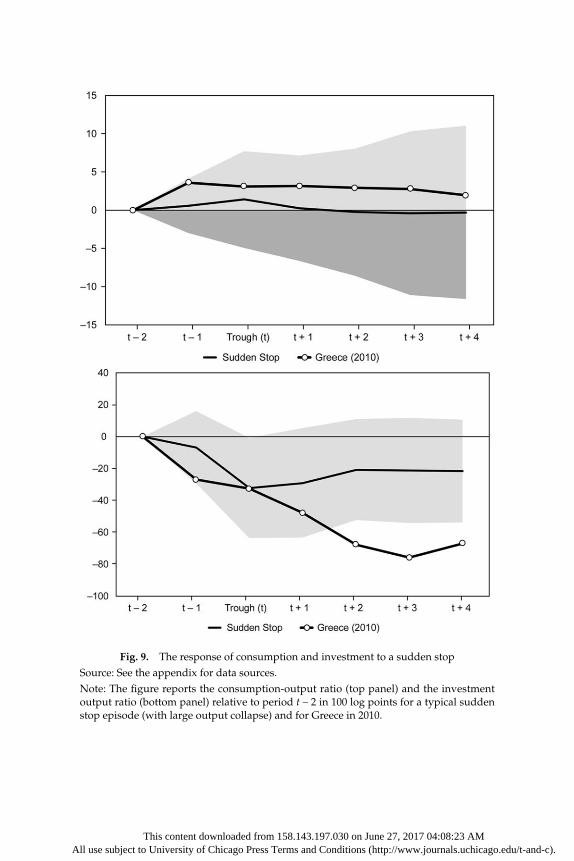
Fig. 9. The response of consumption and investment to a sudden stopSource: See the appendix for data sources.Note: The figure reports the consumption- output ratio (top panel) and the investment output ratio (bottom panel) relative to period t – 2 in 100 log points for a typical sudden stop episode (with large output collapse) and for Greece in 2010.
This content downloaded from 158.143.197.030 on June 27, 2017 04:08:23 AMAll use subject to University of Chicago Press Terms and Conditions (http://www.journals.uchicago.edu/t-and-c).

24 Gourinchas, Philippon, and Vayanos
gate this, figure 10 reports the average output response to each of the following shocks: a sovereign default, a lending boom/bust, as well as the trifecta shock that consists of these two shocks occurring during a sudden stop episode. As an additional point of comparison, the figure also includes the average output response for Ireland, Italy, Portugal, and Spain, that is, the other peripheral countries most affected by the Eurozone crisis (under the label IIPS). Finally, the graph also includes 10% point- wise, one- sided confidence intervals for the trifecta shocks.
The figure illustrates how much of an outlier the Greek crisis truly was. While output per capita initially declined in line with that of a trifecta crisis, by 2011 (i.e., t + 1) output had declined significantly more and kept falling. By contrast, in a typical trifecta crisis, output is back to its pre- crisis level by t + 3. The figure allows us to make a number of additional points. First, trifecta crises are more severe than a typi-cal default crisis, although the differences are small and often insignifi-cant. Second, following a lending boom, output keeps growing. This is because many lending booms in our sample are not always followed by an economic downturn or crisis, as noted also by Gourinchas et al.
Fig. 10. The response of output to various crisesSource: See the appendix for data sources.Note: The figure reports the mean output per capita relative to period t – 2 in 100 log points for various episodes, and for Greece in 2010; 10% one- sided, point- wise confidence intervals for trifecta episodes.
This content downloaded from 158.143.197.030 on June 27, 2017 04:08:23 AMAll use subject to University of Chicago Press Terms and Conditions (http://www.journals.uchicago.edu/t-and-c).

The Analytics of the Greek Crisis 25
(2001) and Ranciere, Tornell, and Westermann (2008). Lastly, the trajec-tory for the IIPS countries illustrates that, in these countries too, the crisis has been much more persistent then expected, with output still 7% below the pre- crisis level as of 2014 (t + 4).
Claim 3. The collapse in Greek output per capita has been significantly more severe and more persistent than the typical trifecta crisis.
Figure 11 makes the same point even more vividly. The panel on the left reports the output trajectory for all countries that experienced a sud-den stop in our sample. The panel on the right presents similar results for all trifecta episodes. Both panels also report the Greek 2010 episode. As is clear from both figures, Greece’s economic performance is cumu-latively much worse than all episodes from the last 35 years, including crises such as Argentina in 2001 or Uruguay in 1983, with the single exception of the United Arab Emirates crisis of 2009.20
We next consider the role of the exchange rate regime. Our data set includes information on the de facto exchange rate regime from Reinhart and Rogoff (2004) and Ilzetzki et al. (2010). We use this data to construct an indicator of the exchange rate regime in the year of the shock and the preceding year (peg/float). We further subdivide pegs based on whether countries maintain their peg for at least two years after the crisis (strict peggers) or abandoned it (de- peggers).21 Figure 12 contrasts the output response following an emerging market sudden stop for de- peggers, strict peggers, and floaters, together with that of Greece and of the IIPS countries. The figure also includes 10% point- wise, one- sided confidence intervals for strict peggers. Unsurprisingly, we find that strict peggers experience a worse adjustment than de- peggers, who in turn perform worse than floaters: by t + 4, output is still 4% below its pre- crisis level for strict peggers, while it is 3% (resp. 8%) above its trend for de- peggers (resp. floaters): a more flexible exchange rate regime is associated with a less severe and less persistent crisis. Greece’s experience is very singular in that respect as well: its output loss is much larger and significantly more persistent than for countries that maintained their exchange rate. By contrast, the experience of the IIPS countries is more in line with that of strict peggers, albeit less severe in 2010 and 2011 (t and t + 1).
There are two ways to think about this result. One possible inter-pretation is that the severity of the Greek crisis cannot be attributed entirely to the strictures of the common currency, since it significantly underperformed other “strict fixers.” This would direct our attention toward other features of the Greek economy than just the exchange rate
This content downloaded from 158.143.197.030 on June 27, 2017 04:08:23 AMAll use subject to University of Chicago Press Terms and Conditions (http://www.journals.uchicago.edu/t-and-c).

Fig. 11. The distribution of output responses to sudden stops and trifecta crisesSource: See the appendix for data sources.Note: The figure reports output per capita relative to period t – 2 in 100 log points for each sudden stop episode (top panel), and for each trifecta crises (bottom panel), together with Greece in 2010.
This content downloaded from 158.143.197.030 on June 27, 2017 04:08:23 AMAll use subject to University of Chicago Press Terms and Conditions (http://www.journals.uchicago.edu/t-and-c).

The Analytics of the Greek Crisis 27
regime. This is not the only interpretation. Clearly, countries can and often choose their exchange rate regime in response to the economic environment. Therefore, the sample of strict fixers may consist precisely of countries who stand to lose relatively less from keeping the exchange rate pegged in the aftermath of a sudden stop. This could be the case in particular if these countries were experiencing a relatively modest decline in output. To investigate this question further, figure 13 reports the data for strict fixers alongside that for Estonia, Latvia, and Greece. Both Latvia and Estonia experienced severe recessions following their 2009 sudden stop episode. Estonia’s output per capita declined by 19% between 2007 and 2009, while that of Latvia declined by 17% between 2007 and 2010. Nevertheless, both countries chose to maintain their peg to the euro and “doubled down” by subsequently adopting the com-mon currency in January 2011 for Estonia and January 2014 for Latvia. Overall, both countries have an experience similar to that of the full sample of strict peggers. Yet, it could hardly be argued that the costs
Fig. 12. The role of the exchange rate regimeSource: See the appendix for data sources.Note: The figure reports output per capita relative to period t – 2 in 100 log points for emerging market sudden stops, by exchange rate regime, together with Greece in 2010; 10% one- sided, point- wise confidence intervals for strict peggers.
This content downloaded from 158.143.197.030 on June 27, 2017 04:08:23 AMAll use subject to University of Chicago Press Terms and Conditions (http://www.journals.uchicago.edu/t-and-c).

28 Gourinchas, Philippon, and Vayanos
of maintaining a fixed exchange rate were small for either country. In-stead, their decision to carry forward and adopt the euro can be related to historical and geostrategic reasons, in particular the desire to anchor their country firmly in the West. Both countries, therefore, adopted the euro despite the large short- run costs associated with doing so: the comparison of their trajectory with Greece’s is unlikely to suffer from a strong selection bias. It is therefore interesting that the experience of Greece appears significantly worse than either country.22
Claim 4. The Greek crisis was significantly more severe than the typical emerg-ing market sudden stop, even for countries such as Latvia or Estonia that main-tained a fixed exchange rate in the aftermath of a sudden stop with large output collapse.
Figure 14 reports credit to the nonfinancial sector (left panel) and public debt (right panel), relative to output. The credit- to- output ratio is measured in deviation from a Hodrick- Prescott (HP) filter trend, while the debt- to- output ratio is measured relative to the country mean. Each
Fig. 13. Output response for strict peggersSource: See the appendix for data sources.Note: The figure reports output per capita relative to period t – 2 in 100 log points for emerging market strict peggers, together with Estonia (2009), Latvia (2009), and Greece (2010); one- sided 10% point- wise confidence intervals for strict peggers.
This content downloaded from 158.143.197.030 on June 27, 2017 04:08:23 AMAll use subject to University of Chicago Press Terms and Conditions (http://www.journals.uchicago.edu/t-and-c).

Fig. 14. Credit and government debt Source: See the appendix for data sources.Note: The left panel reports the ratio of credit to the nonfinancial sector to output, in deviation from a Hodrick- Prescott trend, in percent of GDP. The right panel reports the ratio of government debt to output, in deviation from a country mean, in percent of GDP. Both panels report the typical response over each type of episode, together with Greece in 2010; one- sided 10% point- wise confidence intervals for lending boom (top panel) and trifecta (bottom panel).
This content downloaded from 158.143.197.030 on June 27, 2017 04:08:23 AMAll use subject to University of Chicago Press Terms and Conditions (http://www.journals.uchicago.edu/t-and-c).

30 Gourinchas, Philippon, and Vayanos
variable is expressed in percent of GDP. The left panel reports 10% one- sided, point- wise confidence bands for lending boom/bust episodes, while the right panel reports similar confidence bands for trifecta epi-sodes, since these episodes witness the largest increase in public debt. Starting with the credit- to- output ratio, we see that the initial leverage was high, but not as high as in typical lending boom episodes, around 10% of GDP. The ratio of credit to GDP was gradually reduced, al-though at a more measured pace than in typical episodes. Overall, the contraction in credit to the economy is similar to what is observed in other countries. Confidence bands are quite large.
Turning to public debt, we observe an elevated level of public debt even before the crisis (18% of GDP above mean in 2008), increasing rapidly and remaining significantly more elevated than in other episodes. We can see on the graph the effect of the 2012 debt restructuring (in t + 2), reducing the debt- to- output ratio from 80% to 60% of GDP above its mean, but fol-lowed by a subsequent worsening, in part due to the collapse in economic activity in 2013 and 2014. Compared to trifecta or other episodes, levels of public debt remain extraordinarily high and it is clear from this figure that efforts to bring public debt back to sustainable levels have failed.
Claim 5. Domestic leverage in Greece was similar to other lending boom/bust episodes and evolved similarly. By contrast, public debt to output re-mained extremely elevated. Efforts to reduce the public debt burden mostly failed, despite a substantial debt restructuring in 2012.
Figure 15 reports the trade balance- to- output ratio as well as the consumer price index (CPI)- based multilateral real exchange rate com-piled by the IMF. As for domestic credit and public debt, the trade balance- to- output ratio is measured in deviation from country means and expressed in percent of GDP. The multilateral real exchange rate is expressed in percentage deviation from its country mean. The figure also reports 10% point- wise, one- sided confidence intervals for sudden stop episodes. The left panel (trade balance) illustrates the gradual but large improvement of the Greek trade balance between 2008 and 2014, in ex-cess of 10% of GDP, compared to the typical sudden stop episode. Unlike typical sudden stops, where loss of market access forces the trade bal-ance and current account to improve overnight, the overall improvement in Greece was spread out gradually. The cumulated improvement in the trade balance in a typical sudden stop represents 6.2% of output, 5% of which occurs in the year of the sudden stop itself. As discussed in the previous section, financial assistance and access to the liquidity facilities
This content downloaded from 158.143.197.030 on June 27, 2017 04:08:23 AMAll use subject to University of Chicago Press Terms and Conditions (http://www.journals.uchicago.edu/t-and-c).

Fig. 15. Net exports and real exchange rateSource: See the appendix for data sources.Note: The top panel reports the ratio of net exports on goods and services to output, in deviation from country mean, in percent of GDP. The bottom panel reports the multilat-eral real exchange rate in percentage deviation from a country mean. Both panels report the typical response over each type of episode, together with Greece in 2010; one- sided, point- wise confidence intervals for trifecta episodes.
This content downloaded from 158.143.197.030 on June 27, 2017 04:08:23 AMAll use subject to University of Chicago Press Terms and Conditions (http://www.journals.uchicago.edu/t-and-c).

32 Gourinchas, Philippon, and Vayanos
of the European Central Bank allowed Greece to spread out a massive and necessary adjustment in its trade balance. The right panel indicates that most of this adjustment occurred without major movements in the real exchange rate. Like other countries experiencing a sudden stop, Greece’s real exchange rate was initially overappreciated by about 13%. Yet, while the real exchange rate depreciates by 10% in the aftermath of a typical sudden stop (and a massive 35% following a trifecta), Greece’s real exchange rate only depreciated by 4.5% between 2008 and 2014.23
Claim 6. The adjustment of external balances occurred more gradually, but was nevertheless very significant in size. The improvement in external accounts occurred despite any significant movement in the real exchange rate.
IV. Model
This section presents a stylized model of a small open economy in a currency union with rich macrofinancial linkages. The model is de-signed to shed light on two sets of issues. First, we want a realistic enough model that allows us to understand which shocks were respon-sible for the performance of the Greek economy, both before and during the crisis. Second, we want to use the model to perform some simple counterfactual exercises. To achieve these objectives, the model needs to remain stylized. In particular, while we introduce many macrofinance features, we abstract from a full microfounded model of the banking sector that would put excessive constraints on the data. The model fea-tures eight exogenous stochastic processes. They are labeled zs and each is assumed to follow an AR(1) process of the form:
zti = rizt−1
i + s iti, (1)
where the persistence and volatility parameters (ri, si) are estimated from the data, and the innovations ´t
i are i.i.d. with mean zero and unit variance, and i = {dg, spend, . .} is the name of the shock. We next specify the government, households, nonfinancial firms, and the financial sector.
A. Government
Budget Constraint
The government imposes a flat tax on income, spends Gt on goods and services, and makes social transfers Tt. Let B$,t−1
g be the face value (in
This content downloaded from 158.143.197.030 on June 27, 2017 04:08:23 AMAll use subject to University of Chicago Press Terms and Conditions (http://www.journals.uchicago.edu/t-and-c).

The Analytics of the Greek Crisis 33
units of the common currency) of the debt issued at time t – 1 and due at time t. The nominal budget constraint of the government, conditional on not defaulting, is
B$,tg
Rtg + ttPH,tYt = PH,t Gt + Tt( ) + B$,t−1
g , (2)
where PH,t is the price index of home goods (so PH,tYt is nominal GDP), tt is a time- varying tax rate, and Rt
g is the gross interest rate on sover-eign debt. It will be convenient to work with real variables. We define real government debt Bt
g ≡ B$,tg / PH,t. We can then rewrite the budget
constraint (conditional on not defaulting) as
Btg
Rtg + ttYt = Gt + Tt +
Bt−1g
PtH, (3)
where PtH ≡ PH,t / PH,t−1 is the domestic (i.e., PPI) inflation rate from t – 1
to t. This formula makes clear that unexpected inflation at time t lowers the real debt burden. We use this convention for all other nominal assets.
Sovereign Default
Sovereign risk plays an important role in the Greek crisis.24 We do not model an optimal default decision by the government. Instead, we in-troduce a default shock ! t
dg and assume that the default happens when ! tdg < F(Bt−1
g / PtH ;Yt). We assume that the function F is increasing in the
real debt burden Bt−1g / Pt
H and decreasing in real GDP Yt. For instance, F could simply be the ratio of debt to GDP. The expected default rate is Et[ !dt+1] = Pr( ! t+1
dg < F(Btg / Pt+1
H ;Yt+1)|It), where It is the information set of investors at time t. Notice that the distribution of ! t+1
dg can be time varying. What matters most in our model, however, are expected credit losses, which take into account the probability of default and expected loss given default. Upon default, government debt is reduced by some haircut and we let dt
g denote expected credit losses. In our quantitative analysis, we adopt the following log- linear specification for expected credit losses at time t + 1:
dtg = dg
Bg
Y(bt
g − Et[yt+1] − Et[pt+1h ] + zt
dg), (4)
where Bg / Y is the average debt- to- GDP ratio, dg is a sensitivity param-eter, and lowercase variables (e.g., bt
g ) represent log deviations from
This content downloaded from 158.143.197.030 on June 27, 2017 04:08:23 AMAll use subject to University of Chicago Press Terms and Conditions (http://www.journals.uchicago.edu/t-and-c).

34 Gourinchas, Philippon, and Vayanos
steady- state values. The sovereign risk shock ztdg follows an AR(1) as
postulated in equation (1), with persistence rdg and volatility sdg. Equa-tion (4) states that expected default losses increase with the level of debt, decrease with the inflation rate since the latter reduces the real debt burden, and increase with the sovereign default shock zt
dg. We will use data on sovereign yields to estimate the parameters {dg, rdg, sdg}. The rate paid by the government on its debt is then (in log deviations)
rtg = rt + dt
g,
where rt is the international interest rate.
Fiscal Policy
The government’s spending policy and its social transfer policy are rep-resented by the same rule
gt = Flgt−1 − Fnnt − Frrtg − Fbbt
g + ztspend, (5)
where gt is the log deviation of spending, and nt, rtg, and bt
g are log devia-tions of employment Nt, government credit risk spread Rt
g, and govern-ment debt Bt
g from their steady- state values, Fl, Fn, Fr, and Fb are fixed parameters, and zt
spend is a spending shock that follows equation (1) with persistence rspend and volatility sspend.25 We have the same rule for trans-fers tt. We allow spending itself to be autoregressive (with Fl > 0) to cap-ture the fact that government programs are often scheduled for several years. This fiscal rule implies that the fiscal authorities respond to an increase in sovereign debt by tightening expenditures and reducing so-cial transfers. The term Fn captures automatic stabilizers: as the economy deteriorates, fiscal transfers and spending tends to increase. This formu-lation allows government expenditures and transfers to change both be-cause of macro and financial channels, and also because of spending shocks. Lastly, we specify the following process for the tax rate:
tt = t + zttax,
where ztax follows equation (1) with persistence rtax and volatility stax and t is calibrated to the steady state.
B. Households
Household debt dynamics played an important role during the Great Recession, so we need to introduce borrowers and savers in the model.
This content downloaded from 158.143.197.030 on June 27, 2017 04:08:23 AMAll use subject to University of Chicago Press Terms and Conditions (http://www.journals.uchicago.edu/t-and-c).

The Analytics of the Greek Crisis 35
Households are heterogeneous in their time preferences, as in Eggerts-son and Krugman (2012) and Martin and Philippon (2014).26 There are two types of households: a measure 1 − x of patient households in-dexed by i = s (who will be savers in equilibrium), and a measure x of impatient households indexed by i = b (who will be borrowers in equilib-rium). These households have identical preferences over goods and hours worked, but differ in their discount factors: we assume that bs > bb. Household i maximizes expected lifetime utility
E0t=0
∞
∑bit Ct
i( )1−g
1 − g−
Nti( )1+f
1 + w
⎛
⎝⎜
⎞
⎠⎟ ,
where Cit is a bundle of home and foreign goods, defined in Gali and
Monacelli (2008) by
Cti ≡ [(1 − √)1/ehCH,t
i(eh−1)/eh + √1/ehCF,ti(eh−1)/eh]eh/(eh−1),
where eh is the elasticity of substitution between home and foreign goods and √ is the degree of openness of the economy. As usual, the home consumer price index (CPI) is
Pt ≡ [(1 − √)PH,t1−eh + √PF,t1−eh]1/(1−eh).
Household Default
Households borrow at the rate Rth and can default on their debts. Let dth
be the credit loss rate on household loans. Default is a loss for the banks and a positive transfer to borrowers, similar to the financial shock de-scribed in Iacoviello (2015). The borrowers’ budget constraint, following the same convention as with the government, is
PtCtb = (1 − tt)WtNt
b +PH,tBth
Rth
− (1 − dth)PH,t−1Bt−1h + PH,tTtb. (6)
where (1 − tt)WtNtb denotes after- tax labor income, Rt
h the gross interest rate faced by borrowers, Bth is the real face value of the household debt issued at t and due at t + 1, and Ttb the transfers received by borrowers. Borrowers are subject to the following borrowing limit:
Bth <Bth
x.
In our notations, Bth is a per capita measure, while Bth denotes the aggre-gate lending capacity of the financial sector to households. We later de-
This content downloaded from 158.143.197.030 on June 27, 2017 04:08:23 AMAll use subject to University of Chicago Press Terms and Conditions (http://www.journals.uchicago.edu/t-and-c).

36 Gourinchas, Philippon, and Vayanos
rive this lending limit from the lender’s problem, and we anticipate the result that only impatient households borrow in equilibrium. The credit loss rate is assumed to follow the process:
dth = −dhyyt + dhbbth + ztdh, (7)
where ztdh follows equation (1) with persistence rdh and volatility sdh. Equation (7) states that the credit loss rate on household loans increases with their debt level, decreases with output, and increases with a house-hold default shock zdh. We will use data on nonperforming loans to esti-mate {dhy, dhb, rdh, sdh}. Note that dth are realized credit losses at time t, un-like dt
g, which is an expected loss that may or may not materialize at t + 1.The savers’ budget constraint is
PtCts = (1 − tt)WtNt
s + !RtPH,t−1St−1 − PH,tSt + PH,tTts, (8)
where !Rt is the nominal after- tax gross return on savings PH,t–1St–1 at time t and Tts denotes real transfers to savers. This return is a complex object since savers are residual claimants: in equilibrium, they hold shares of firms and of banks, but also deposits, government bonds, and potentially foreign assets. Notice, however, that in equation (3) we have assumed a uniform tax rate on aggregate income, and this is what mat-ters in the end. The savers’ Euler equation is
Et bCt+1
s
Cts
⎛
⎝⎜
⎞
⎠⎟−g !Rt+1
Pt+1
⎡
⎣⎢
⎤
⎦⎥ = 1,
where Pt+1 = Pt+1 / Pt denotes the gross CPI inflation rate from t to t + 1. Finally, in the aggregate, we have
CH,t = xCH,tb + (1 − x)CH,t
s
Ct = xCtb + (1 − x)Ct
s.
Nominal Wage Rigidity
We assume a standard model of wage stickiness with a representative union setting wages à la Calvo. The wage equations are standard and satisfy:
ptw = bEtpt+1
w − lw(wt − gct − wnt) + ztw,
pt = (1 − √)pth + √pt
f ,
wt = wt−1 + ptw − pt
h,
This content downloaded from 158.143.197.030 on June 27, 2017 04:08:23 AMAll use subject to University of Chicago Press Terms and Conditions (http://www.journals.uchicago.edu/t-and-c).

The Analytics of the Greek Crisis 37
where ptw denotes wage inflation, wt is the real wage in terms of the CPI
(ln(Wt / Pt)), ztw is a wage- markup shock that follows equation (1) with persistence rw and volatility sw; pt denotes CPI inflation, pt
h is home inflation, pt
f is foreign inflation, and lw is derived from the Calvo wage- setting process. The first equation is a forward- looking wage Phillips curve. Wage inflation depends on expected future wage inflation, on the marginal rate of substitution between consumption and leisure, and on the wage- markup shock zw.
C. Nonfinancial Firms
We separate firms into goods- producing and capital- producing firms in order to simplify the derivation of the price- setting equation on the one hand, and the investment/Q equation on the other hand.
Capital- Producing Firms
Capital firms convert consumption goods into capital through invest-ment and rent this capital to goods- producing firms for a rental rate Zk,t. The capital stock evolves according to
Kt = (1 − d)Kt−1 + It, (9)
and real period profits (i.e., scaled by PH,t) for these firms are given by
Divt = Zk,tKt−1 − It −wk
2Kt−1
ItKt−1
− d⎛
⎝⎜
⎞
⎠⎟2
,
where the last term captures adjustment costs to physical capital. Let Rtk
be the firm’s funding cost. The real value of capital- producing firms is V(Kt–1) and satisfies the following Bellman equation
V(Kt−1) = maxIt,Kt
Zk,tKt−1 − It −wk
2Kt−1
ItKt−1
− d⎛
⎝⎜
⎞
⎠⎟2
+ EtPH,t+1
Rtk
V(Kt)⎡
⎣⎢⎤
⎦⎥⎧⎨⎪
⎩⎪
⎫⎬⎪
⎭⎪
subject to equation (9).Let xt ≡ (Kt − Kt−1) / Kt−1 be the net investment rate. Given our ho-
motheticity assumptions, we guess and verify that the value function can be written as
V Kt−1( ) = VtKt−1,
where
This content downloaded from 158.143.197.030 on June 27, 2017 04:08:23 AMAll use subject to University of Chicago Press Terms and Conditions (http://www.journals.uchicago.edu/t-and-c).

38 Gourinchas, Philippon, and Vayanos
Vt = maxxt
Zk,t − xt − d − wk
2xt2 + 1 + xt( ) Et
PH,t+1
RtkVt+1
⎡
⎣⎢⎤
⎦⎥⎧⎨⎩
⎫⎬⎭
. (10)
Define Tobin’s Q as the end- of- period value of assets divided by the end- of- period replacement cost of capital
Qt ≡ EtPH,t+1
RtkVt+1
⎡
⎣⎢⎤
⎦⎥. (11)
Optimal investment yields the standard Q- equation:
xt =Qt − 1
wk
. (12)
Goods- Producing Firms
Goods- producing firms produce differentiated varieties of a domestic good using capital and labor. The production function for a producer of good j is
Yt( j) = AKt( j)aNt( j)1−a,
where A is aggregate total factor productivity (TFP). We focus here on the case where TFP is constant because the model is simpler to present and fits the data quite well. Goods- producing firms are subject to a fi-nancial friction that requires them to pay part of their operating costs in advance, before production is undertaken, as in Christiano, Eichen-baum, and Evans (2005) or Jermann and Quadrini (2012).27 Let csk de-note the fraction of input cost that needs to be financed by working capital loans. Profits are given by
Profitst = Revenuest − Costst[1 + csk(Rtk − 1)].
Standard cost minimization yields an expression for the nominal mar-ginal cost,
MCt$ = [1 + csk(Rt
k − 1)]A
PH,tZk,t
a( )a Wt
1 − a( )1−a
.
Notice that the working- capital friction can be represented by an incre-mental marginal cost for the firm. This will be an important property, as it allows financial frictions to pass through to inflation. Differentiated goods producers solve a standard Calvo problem, given factor de-mands. Given real marginal cost MCt ≡ MCt
$ / PH,t, we can write the (log- linear) Phillips curve as
This content downloaded from 158.143.197.030 on June 27, 2017 04:08:23 AMAll use subject to University of Chicago Press Terms and Conditions (http://www.journals.uchicago.edu/t-and-c).

The Analytics of the Greek Crisis 39
ph,t = lpmct + bEtph,t+1 + ztph,
where lp is derived from the Calvo price- setting process, b is the dis-count factor of savers, and the (log) real marginal cost is
mct =cskRk
1 + csk(Rk − 1)rtk + azk,t + (1 − a)(wt + √tott);
ztph is an AR(1) price markup shock that satisfies equation (1) with
persistence rph and volatility sph. Notice that marginal costs are de-flated in terms of the price of home- produced goods, hence the terms- of- trade adjustment for the real wage, which reflects the term Pt / PH,t. Finally, we have the usual static optimality condition for la-bor demand:
Kt−1
Nt
= a
1 − a
Wt
PH,tZk,t
.
D. Banks, Sudden Stop, and Funding Cost
A fully specified model of banking intermediation as in Gertler and Kiyo taki (2010) is beyond the scope of this paper. Moreover, the financial- sector data necessary to estimate the restrictions of such a model, such as the balance sheet of banks and its components, are not available (see Faria- e- Castro [2016] for a more ambitious estimation). There is, how-ever, one fundamental insight from the models of banking intermedia-tion that is theoretically straightforward and, as we show later, em-pirically relevant. At the heart of many banking models is a capital requirement of the type
Vtbank ≥ k
Btk
Rtk+ Bth
Rth
⎛
⎝⎜
⎞
⎠⎟, (13)
where Vtbank is the franchise value of the banking sector and Btk and Bth
denote the outstanding loans to the corporate nonfinancial and house-hold sectors, respectively, both measured at the end of period t. This equation assumes that there is no capital requirement for sovereign ex-posure, as was the case in Europe at the time. Equation (13) says that bank equity Vt
bank must cover a fraction k of the total credit exposure to firms and to households. The second important equation is the current account of the banking sector:
PH,t+1Et+1 = (1 − dt+1k )Btk + (1 − dt+1h )Bth − Dt . (14)
This content downloaded from 158.143.197.030 on June 27, 2017 04:08:23 AMAll use subject to University of Chicago Press Terms and Conditions (http://www.journals.uchicago.edu/t-and-c).
40 Gourinchas, Philippon, and Vayanos
Equation (14) states that nominal bank earnings PH,t+1Et+1 consist of re-payment from firms and households net of default losses, minus the repayment of banks’ liabilities Dt. Finally, bank value solves a Bellman equation
Vtbank = max
Bt{ },DtDivt + Et
Lt+1
Pt+1
PH,t+1((1 − s)Et+1 + sVt+1bank)
⎡
⎣⎢⎤
⎦⎥, (15)
where s is an exogenous exit rate, Lt+1 is the pricing kernel of savers, and dividends Divt are assumed to be a fixed fraction of earnings Et. This captures the assumption that banks cannot raise equity very quickly, and it implies that capital losses lead to tighter lending con-straints, as least in the short run.
Equations (13), (14), and (15) capture the fundamental credit channel in the economy. Credit losses reduce banks’ earnings in equation (14), lower bank value in equation (15), and tighten capital requirement in equation (13). This leads to an increase in the economy’s funding cost. All else equal, this channel is stronger the higher the bank leverage. We capture this idea in two steps. First, we model the banks’ (log) funding cost rtd as
rtd = rt + ztr + jdLEt[dt+1
p ],
where L is bank leverage (assets over equity capital) in steady state, jd is a sensitivity parameter to be estimated, dt+1
p measures losses on private credit portfolio (households and firms’ loans), and ztr is a sudden stop shock that increases funding costs to banks; zr satisfies equation (1) with persistence rr and volatility sr. Since we only have data on total nonper-forming loans, we will assume that loss rates on households’ and firms’ credit are identical: dth = dtk ≡ dt
p.Second, we assume that banks’ funding costs are passed on to banks’
customers (with a constant margin that drops out in logs), therefore
rtk = rtd.
Note that in our notations above, rtk is the funding cost of firms, which enters directly the Q equations (10) and (11). For households, we had defined rth as the interest rate on loans, gross of expected losses, that enters the budget constraint (6). If we were to quote an interest rate for corporate loans, it would be rtd + Et[dt+1k ], and the expected return would be rtd. With our assumptions, the sudden stop shock is an increase in the country’s funding cost above and beyond what can be explained by domestic intermediation spreads.
This content downloaded from 158.143.197.030 on June 27, 2017 04:08:23 AMAll use subject to University of Chicago Press Terms and Conditions (http://www.journals.uchicago.edu/t-and-c).
The Analytics of the Greek Crisis 41
E. Equilibrium
All transactions with the rest of the world happen at rate Rt. Let NFAt denote the net foreign assets of the country (in units of domestic goods). By definition, NFA evolves as
NFAt
Rt
= NFAt−1 − PtCt + PH,t Yt − Gt − It −wk
2Kt−1
Kt
Kt−1
− 1⎛
⎝⎜
⎞
⎠⎟2⎛
⎝⎜⎜
⎞
⎠⎟⎟.
As is common in the literature, we make a technical assumption to en-sure stationarity of NFA.28 We assume that there is a (small) price im-pact of NFA on the country’s borrowing (or saving) rate
∂logRt
∂logNFAt
= −er,
where er is a small but strictly positive number. Clearing in the market for domestic goods requires
Yt = CHt +PHtPtF
⎛
⎝⎜
⎞
⎠⎟−e f
CtF + Gt + It +
wk
2Kt−1
Kt
Kt−1
− 1⎛
⎝⎜
⎞
⎠⎟2
,
where CtF represents aggregate foreign consumption and Pt
F the foreign CPI; e f is the demand elasticity.
Household Debt
Banks lend to domestic households. We assume that borrowers are im-patient enough to hit their borrowing limits, so
xBth = Bth.
The basic model does not pin down a unique borrowing rate Rth.
As long as Rth > Rt
d , banks are willing to lend more. As long as bbEt[(Rt
h / Pt+1)u(ct+1)] < u(ct) borrowers want to borrow more. In steady state, any Rh ∈ (bs
−1,bb−1) is potentially an equilibrium.29 This issue is
present in and out of steady state. For the steady state, however, a rea-sonable assumption is that the lending spread is pinned down by free entry into banking. We will directly calibrate the steady- state spread Dt ≡ Rt
h / Rt using empirical studies of financial intermediation: Philip-pon (2012) shows that the spread is remarkably stable in the long run at D = 1.02. Out of steady state, we expect both loan supply and loan de-mand to decrease in response to an increase in banks’ funding cost, so we specify in log deviations from steady- state values
This content downloaded from 158.143.197.030 on June 27, 2017 04:08:23 AMAll use subject to University of Chicago Press Terms and Conditions (http://www.journals.uchicago.edu/t-and-c).

42 Gourinchas, Philippon, and Vayanos
bth = cbhbt−1h − jbhrtd + ztbh, (16)
where ztbh is an AR(1) shock that satisfies equation (1) with persistence rbh and volatility sbh.
Interest Rates and Funding Costs in the Model
There are four interest rates in the model, so it is useful to summarize them here. First of all, there is the baseline interest rate rt that enters the NFA and the Euler equation of savers. Above and beyond this rate there are spreads and expected losses, so that
rtd = rt + ztr + jdLEt dt+1
p[ ]
dtp = −dyyt + dbbt−1 + zt
def
rtk = rtd
rth = rtd + Et dt+1p[ ]
rtg = rt + dt
g
dtg = dg
Bg
Ybtg − Et yt+1[ ] − Et pt+1
h[ ] + ztdg( )
.
Notice our assumptions here. First, domestic savers do not earn higher expected returns when there is a sudden stop. They earn r, which re-mains essentially constant and equal to the rate in the Eurozone. Sec-ond, the banks are sensitive to the sudden stop and to credit losses. The sudden stop ztr enters the economy via the banks, which then pass it on to their customers. Nonperforming loans dt+1
p hurt banks and increase the funding costs of all private agents. We only have data on total non-performing loans, so we do not model separately firm and household defaults. We assume that they move together and we estimate only one equation for dt
p. The shock ztdef captures the evolution of NPLs that is not
predicted by macroeconomic fundamentals.Fourth, the government is not necessarily affected by the same sud-
den stop as the private sector. The shock ztdg raises the cost of funds for
the government. It captures pessimism by investors about the credit-worthiness of the government, whether or not this pessimism is borne out in equilibrium. There are many reasons why zt
dg and ztr are different, but let us just mention two. First, as we discussed, the ECB provided funding to Greek banks both directly and indirectly via emergency li-
This content downloaded from 158.143.197.030 on June 27, 2017 04:08:23 AMAll use subject to University of Chicago Press Terms and Conditions (http://www.journals.uchicago.edu/t-and-c).

The Analytics of the Greek Crisis 43
quidity assistance, insulating them from sovereign risk, in particular during the sovereign debt restructuring. Second, government debt is now largely held by official creditors, rather than domestic banks, at-tenuating the link between sovereign and banking risks.
Finally, while the two shocks zrand zdg are conceptually distinct, the model features important feedback loops between the sovereign and the banks. This “doom loop” has been extensively discussed in policy circles and analyzed in stylized models (see Brunnermeier et al. 2016; Farhi and Tirole 2016). The impact of banks on the sovereign is always present via general equilibrium effects and tax revenues. If banks expe-rience a sudden stop, the economy contracts and credit risk, both private and sovereign, increases. Conversely, if sovereign risk increases, the worsening of economic outcomes increases default in the private sector, affecting bank values. Hence, our model features rich and com-plex interactions between the financial and public sectors.
V. Estimation
In this section, we describe the estimation of the model. We combine the Kalman Filter with Bayesian techniques, which allow us to recover estimates for the structural shocks that affected Greece during the first decade of the twenty- first century. These estimated shocks can then be used to conduct counterfactual exercises.
A. Data, Observables, and Calibration
The sample is annual, from 1999 to 2015. Figure 16 shows the eight series that we feed into the model, all measured in log deviations from steady state. For interest rates and inflation, we also take the difference from the Eurozone average series.
The model features as many shocks as observables, which are de-scribed in table 4.30 In addition, we allow for measurement error to do-mestic inflation, wage inflation, and the measure of nonperforming loans since these variables are quite noisy and/or measured impre-cisely. Specifically, we assume that we observe !xt, where
!xt = xt + ´terror
and terror is a measurement error term.31 For household debt, we take as
a proxy the series for total credit to the private nonfinancial sector for Greece.
This content downloaded from 158.143.197.030 on June 27, 2017 04:08:23 AMAll use subject to University of Chicago Press Terms and Conditions (http://www.journals.uchicago.edu/t-and-c).

44 Gourinchas, Philippon, and Vayanos
We estimate the remaining “dynamic” parameters using standard Bayesian estimation techniques following An and Schorfheide (2007).32 We estimate a total of 25 parameters: the persistence and volatility of the eight structural shocks, the variance of the three measurement er-rors, as well as six other dynamic parameters: the elasticity of expected
Fig. 16. Observables: Filtered dataNote: All series are in log deviations from steady state. Interest rates and inflation rates are also in deviation from the Eurozone average. The NPL, GDP deflator, and wages are assumed to be measured with errors.
Table 4Observables and Shocks
Observable Description Shock Shock Description
Gt + Tt Government spending ztspend Govt. spending shock
ttYt Government revenues zttax Tax rate shock
Rtg Greek government spread over
EZ averageztdg Sovereign risk shock
Rtk SME spread over EZ average zt
r Funding cost shockexp(dt
p) Nonperforming loans/total loans, def = npl
zdef Private default shock
Pt Greece CPI – EZ CPI zph PPI cost push shockBth Household debt zt
bh Household credit shockPt
w
Greek wage inflation – EZ wage inflation
zw
Wage inflation shock
Note: We use a combination of calibration and estimation. We calibrate parameters that affect steady- state variables. Most of the calibrated parameters take standard values for small open economies and are reported in tables A5, A6, and A7 in the ap-pendix.
This content downloaded from 158.143.197.030 on June 27, 2017 04:08:23 AMAll use subject to University of Chicago Press Terms and Conditions (http://www.journals.uchicago.edu/t-and-c).

The Analytics of the Greek Crisis 45
sovereign default losses with respect to debt to GDP, the elasticities of private default with respect to GDP and debt, the persistence of the household credit equation, the elasticity of household credit with re-spect to the cost of funds, and the pass- through of future default to current lending rates. The estimation results, along with our choice of priors, are described in table A9 in the appendix.
B. Results
Smoothed Variables
The smoothed shocks are reported in figure A2 in the appendix. We also use the Kalman Filter to extract the sequences implied by the model for the remaining endogenous variables. This provides a good way of gaug-ing the fit of the model. We present the most important series in figure 17,
Fig. 17. Smoothed variablesNote: The figure reports the model estimated values of output, investment, inflation (price and wage), and next exports- to- GDP ratio. Both inflation series are part of the esti-mation, but are assumed to be measured with error.
This content downloaded from 158.143.197.030 on June 27, 2017 04:08:23 AMAll use subject to University of Chicago Press Terms and Conditions (http://www.journals.uchicago.edu/t-and-c).

46 Gourinchas, Philippon, and Vayanos
where we plot the data and model- implied paths for GDP, corporate in-vestment, PPI inflation, and current account- to- GDP ratio.
The main point to take away from figure 17 is that the model’s pre-dictions for output and investment are good, even though we did not use any data on output or investment in the estimation. This means that our fiscal and financial multipliers are consistent with the data. For domestic price inflation, whose measurement is imperfect, we plot the observed raw data series against the model- based series that filters out the noise.33 For wage inflation, on the other hand, measurement errors appear small.
Figures 18–21 are the first main findings of the model. In each case, the black line is the smoothed value of the corresponding endogenous variable, in percent deviations from steady state. Each bar represents the contribution of a corresponding shock and its lagged values to the predicted value of the corresponding variable at each point in time.34
GDP
The GDP series in figure 18 shows how our model interprets the Greek crisis. Around 2000, credit demand is high and credit risk is low, so households borrow and consume. During that period, government spending increases more than predicted by our fiscal rule, as captured by the positive spending shocks. This is the same finding as in Martin and Philippon (2014). This massive fiscal expansion explains most of the output gap, which is around +15% in 2007. The recessionary shocks arrive in sequence. The model finds that the sudden stop starts in 2009 and remains very significant until 2013, depressing output by 5% to 10%. It is important to keep in mind that this is a decomposition with respect to shocks, not propagation mechanisms. For example, the sud-den stop shock appears first in the funding cost of the private sector, but its effects propagate via several mechanisms: lower credit, lower demand, more private and sovereign default risk, and so forth. The ef-fect of all of these mechanisms is aggregated into the bar corresponding to the sudden stop shock (right- slanted dashed line).
Role of Government Spending
It is important to understand how exactly the model interprets fiscal policy shocks. We feed in actual government spending in our calibra-tion, and since the model implies significant fiscal multipliers (around
This content downloaded from 158.143.197.030 on June 27, 2017 04:08:23 AMAll use subject to University of Chicago Press Terms and Conditions (http://www.journals.uchicago.edu/t-and-c).
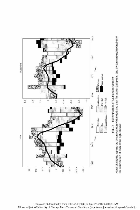
Fig.
18.
D
ecom
posi
tion
of G
DP
and
inve
stm
ent
Not
e: T
he fi
gure
repo
rts
the
dec
ompo
siti
on o
f the
pre
dic
ted
pat
h fo
r ou
tput
(lef
t pan
el) a
nd in
vest
men
t (ri
ght p
anel
) int
o th
e co
ntri
buti
on o
f eac
h of
the
eigh
t sho
cks.
This content downloaded from 158.143.197.030 on June 27, 2017 04:08:23 AMAll use subject to University of Chicago Press Terms and Conditions (http://www.journals.uchicago.edu/t-and-c).

48 Gourinchas, Philippon, and Vayanos
1.5), fiscal dynamics “accounts” for much of GDP dynamics. But that is not how the model computes the contribution of each shock. The model seeks to understand why government spending moves using the fiscal rule (5). Government default risk increases in 2011 and especially in 2012, the year of the sovereign default. From 2010 to 2012, there is no au-tonomous negative spending shock. In other words, the observed path of government spending can be explained by our fiscal rule, given the increase in funding costs.35 In reality, spending was largely determined by official financing. Under the 2010 program, the Greek government received 110 billion euros. Another 130 billion euros became available as part of the 2012 program and debt restructuring. What the model says is that the size of the program (and the implied path of spending and taxes) was consistent with a fiscal rule such as equation (5).
Autonomous (negative) spending shocks emerge in 2013, and to a lesser extent in 2014, because sovereign spreads decrease and spending does not increase (or even decreases). This coincides with the imple-mentation of the 2012 IMF and Eurogroup program.
Figure 19 reports the decomposition for government debt (left panel) and its yield (right panel). Both variables are part of the estimation. We see that the accumulation of government debt is mostly the conse-quence of past spending decisions. Fiscal expansions do not increase debt much in the short run because GDP and revenues increase. In the long run, however, they increase debt. The debt accumulation after the crisis in figure 19 is mostly due to spending shocks that happened before the crisis. The yield on sovereign debt is also mostly affected by the fiscal shock, and also by sovereign risk. We observe a sharp decline in sovereign risk following the 2012 debt restructuring.
Markups and Nonperforming Loans
Finally, starting in 2013, two important factors dragging down the Greek economy are the rise in nonperforming loans and the increase in price markups. As in Agatha Christie’s Murder on the Orient Express, the boom and bust in Greek output per capita cannot be attributed to a single cause: over time, different shocks played a role. This decom-position also indicates that, by 2015, the external drags on the Greek economy due to the sudden stop and the sovereign debt crisis have sub-sided. What remains are mostly domestic factors: some fiscal austerity, mounting losses on private loans, and the relative lack of adjustment in Greek prices relative to wages.
This content downloaded from 158.143.197.030 on June 27, 2017 04:08:23 AMAll use subject to University of Chicago Press Terms and Conditions (http://www.journals.uchicago.edu/t-and-c).

Fig.
19.
D
ecom
posi
tion
of g
over
nmen
t deb
t and
yie
ldN
ote:
The
figu
re re
port
s th
e d
ecom
posi
tion
of t
he p
red
icte
d p
ath
for
sove
reig
n d
ebt (
left
pan
el) a
nd th
e yi
eld
on
sove
reig
n d
ebt (
righ
t pan
el) i
nto
the
cont
ribu
tion
of e
ach
of th
e ei
ght s
hock
s.
This content downloaded from 158.143.197.030 on June 27, 2017 04:08:23 AMAll use subject to University of Chicago Press Terms and Conditions (http://www.journals.uchicago.edu/t-and-c).

50 Gourinchas, Philippon, and Vayanos
Investment (figure 18, right panel) is mostly affected by the increase in funding costs due to the sudden stop in 2009–2013. In 2014 and 2015, investment remains subdued largely because of private- sector credit risk, fiscal austerity, and especially price markup shocks.
Figure 20 reports both expected private defaults (left panel) and the funding cost of the private sector (right panel). Both variables are also perfectly predicted by the model, by construction. Private credit losses were low early in the sample because of low private default risk and the strong stimulus coming from government spending. After 2007, private credit losses mount rapidly, mostly as a consequence of macrodynam-ics. The increase in funding costs due to the sudden stop, the collapse in credit demand, fiscal austerity, and the increase in private default risk all contribute to raise private credit losses. The right panel illustrates that the main driver of private sector cost of funds was the sudden stop.36
Figure 21 reports government spending (left panel) and revenues (right panel). Government spending is largely autonomous in the boom, a finding consistent with Martin and Philippon (2014). In the bust, it is explained by the funding constraint, and then by restrictions consistent with the IMF/Eurogroup program. Government revenues are dominated by macrodynamics. While tax shocks move from nega-tive to positive, revenues decline overall due to the sudden stop and its effect on output and investment, the impact of spending cuts on output, and mounting nonperforming loans.
Finally, figure 22 decomposes domestic price (left panel) and wage inflation (right panel). Fiscal austerity, private sector default, and wage compression (negative wage markup shocks) contribute to deflationary price and wages forces. Yet wage adjustment is significantly larger than price adjustment, and the difference can largely be attributed to price markup shocks zph.
C. Impulse Responses
We next explore the internal mechanics of the model by plotting some impulse response functions, estimated at the posterior mean of the pa-rameters. Each impulse response reports the effect of a one standard deviation shock on the variables of the model, expressed in percent deviation from their steady state. We present here only a few impulse responses. Other figures are in the appendix.
Figure 23 shows the response to a transfer shock, tspend. Our model is not
Ricardian. An increase in government spending raises the consumption
This content downloaded from 158.143.197.030 on June 27, 2017 04:08:23 AMAll use subject to University of Chicago Press Terms and Conditions (http://www.journals.uchicago.edu/t-and-c).

Fig.
20.
D
ecom
posi
tion
of p
riva
te d
efau
lt a
nd fu
ndin
g co
stN
ote:
The
figu
re re
port
s th
e d
ecom
posi
tion
of t
he p
red
icte
d p
ath
for
hous
ehol
d c
red
it lo
sses
(lef
t pan
el) a
nd th
e bo
rrow
ing
rate
(rig
ht p
anel
) int
o th
e co
ntri
buti
on o
f eac
h of
the
eigh
t sho
cks.
This content downloaded from 158.143.197.030 on June 27, 2017 04:08:23 AMAll use subject to University of Chicago Press Terms and Conditions (http://www.journals.uchicago.edu/t-and-c).

52
Fig.
21.
D
ecom
posi
tion
of g
over
nmen
t spe
ndin
g an
d r
even
ues
Not
e: T
he fi
gure
rep
orts
the
dec
ompo
siti
on o
f the
pre
dic
ted
pat
h fo
r go
vern
men
t spe
ndin
g (l
eft p
anel
) and
gov
ernm
ent
reve
nues
(rig
ht p
anel
) int
o th
e co
ntri
buti
on o
f eac
h of
the
eigh
t sho
cks.
This content downloaded from 158.143.197.030 on June 27, 2017 04:08:23 AMAll use subject to University of Chicago Press Terms and Conditions (http://www.journals.uchicago.edu/t-and-c).

53
Fig.
22.
D
ecom
posi
tion
of d
omes
tic
pric
e an
d w
age
infl
atio
nN
ote:
The
figu
re r
epor
ts th
e d
ecom
posi
tion
of t
he p
red
icte
d p
ath
for
dom
esti
c pr
ice
and
wag
e in
flat
ion
into
the
cont
ribu
-ti
on o
f eac
h of
the
eigh
t sho
cks.
This content downloaded from 158.143.197.030 on June 27, 2017 04:08:23 AMAll use subject to University of Chicago Press Terms and Conditions (http://www.journals.uchicago.edu/t-and-c).

Fig.
23.
Fi
scal
exp
ansi
on s
hock
Not
e: T
he fi
gure
rep
orts
90%
Bay
esia
n co
nfid
ence
ban
ds.
This content downloaded from 158.143.197.030 on June 27, 2017 04:08:23 AMAll use subject to University of Chicago Press Terms and Conditions (http://www.journals.uchicago.edu/t-and-c).

The Analytics of the Greek Crisis 55
of borrowers, as well as output, employment, investment, and inflation. As the economy expands, nonperforming loans decline. Over time, public debt gradually increases, which pushes up sovereign yields. The model thus features a significant but temporary effect of a fiscal expan-sion on output, and a long- lasting effect on the level of public debt.
Figure 24 shows the response to a sovereign risk shock, tdg . The fiscal
rule forces a cut in spending that leads to a drop in output, employ-ment, and inflation. The decline in output increases private credit risk, which feeds back into funding costs and curtails investment. Figure 24 (and figure A3 in the appendix, which looks at the response to a private default shock) illustrates the sovereign/bank interactions: as sovereign risk increases, the funding costs of the private sector are affected. Con-versely, as private default risk increases, sovereign risk increases as well. In our model, these effects work via general equilibrium effects.
Finally, figure 25 shows the response to a sudden stop, r . An increase in the country’s funding cost causes corporate investment to decline. Impatient household debt declines as well, and so does borrower con-sumption. The decline in consumption and investment drives output, employment, and inflation down. The interest rate on government debt increases because the decline in economic activity heightens sovereign risks.
VI. Counterfactuals
In this section, we run five counterfactual exercises. To understand our counterfactual exercises, let yit denote the observation of variable i at date t, and let xit denote the smoothed value for variable i at date t. Let xiT ≡ {xi,t}t=0T denote the estimated smoothed sequence for variable i in our sample period for t = 0, . . . ,T and denote xT the sequence of all smoothed variables: xT ≡ {xiT}. Every estimated sequence can be written as a mapping G(.) from the estimated parameters Q and the sequences of smoothed shocks, {ˆ kT}k=1K ≡ {ˆ k,t}k=1,t=0K,T , where K is the number of shocks in our model:
xT = G(Q, {ˆ kT}k=1K ).
A counterfactual exercise consists in postulating an alternate choice for Q and {ˆ kT}k=1K , denoted !Q and {! kT}k=1K and then compute the counterfac-tual !xT as:
!xT = G( !Q, {! kT}k=1K ).
This content downloaded from 158.143.197.030 on June 27, 2017 04:08:23 AMAll use subject to University of Chicago Press Terms and Conditions (http://www.journals.uchicago.edu/t-and-c).

56
Fig.
24.
So
vere
ign
risk
sho
ckN
ote:
The
figu
re r
epor
ts 9
0% B
ayes
ian
confi
den
ce b
and
s.
This content downloaded from 158.143.197.030 on June 27, 2017 04:08:23 AMAll use subject to University of Chicago Press Terms and Conditions (http://www.journals.uchicago.edu/t-and-c).

57
Fig.
25.
Su
dd
en s
top
Not
e: T
he fi
gure
rep
orts
90%
Bay
esia
n co
nfid
ence
ban
ds.
This content downloaded from 158.143.197.030 on June 27, 2017 04:08:23 AMAll use subject to University of Chicago Press Terms and Conditions (http://www.journals.uchicago.edu/t-and-c).
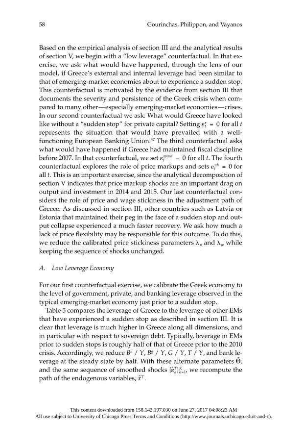
58 Gourinchas, Philippon, and Vayanos
Based on the empirical analysis of section III and the analytical results of section V, we begin with a “low leverage” counterfactual. In that ex-ercise, we ask what would have happened, through the lens of our model, if Greece’s external and internal leverage had been similar to that of emerging- market economies about to experience a sudden stop. This counterfactual is motivated by the evidence from section III that documents the severity and persistence of the Greek crisis when com-pared to many other—especially emerging- market economies—crises. In our second counterfactual we ask: What would Greece have looked like without a “sudden stop” for private capital? Setting t
r = 0 for all t represents the situation that would have prevailed with a well- functioning European Banking Union.37 The third counterfactual asks what would have happened if Greece had maintained fiscal discipline before 2007. In that counterfactual, we set t
spend = 0 for all t. The fourth counterfactual explores the role of price markups and sets ´t
ph = 0 for all t. This is an important exercise, since the analytical decomposition of section V indicates that price markup shocks are an important drag on output and investment in 2014 and 2015. Our last counterfactual con-siders the role of price and wage stickiness in the adjustment path of Greece. As discussed in section III, other countries such as Latvia or Estonia that maintained their peg in the face of a sudden stop and out-put collapse experienced a much faster recovery. We ask how much a lack of price flexibility may be responsible for this outcome. To do this, we reduce the calibrated price stickiness parameters lp and lw while keeping the sequence of shocks unchanged.
A. Low Leverage Economy
For our first counterfactual exercise, we calibrate the Greek economy to the level of government, private, and banking leverage observed in the typical emerging- market economy just prior to a sudden stop.
Table 5 compares the leverage of Greece to the leverage of other EMs that have experienced a sudden stop as described in section III. It is clear that leverage is much higher in Greece along all dimensions, and in particular with respect to sovereign debt. Typically, leverage in EMs prior to sudden stops is roughly half of that of Greece prior to the 2010 crisis. Accordingly, we reduce Bh / Y, Bg / Y, G / Y, T / Y, and bank le-verage at the steady state by half. With these alternate parameters !Q, and the same sequence of smoothed shocks {ˆ kT}k=1K , we recompute the path of the endogenous variables, !xT .
This content downloaded from 158.143.197.030 on June 27, 2017 04:08:23 AMAll use subject to University of Chicago Press Terms and Conditions (http://www.journals.uchicago.edu/t-and-c).

The Analytics of the Greek Crisis 59
Figure 26 reports the path for the actual data (solid line), the smoothed original estimates (tightly dotted line) and the coun-terfactual (dotted line). In this counterfactual, Greece would have been much more constrained in the build- up phase of the crisis. The smaller size of its government sector would have prevented it from excessively stimulating its economy, reducing the output gap from +14.1% in 2007 in the smoothed estimates to +9.2% (top- left panel). Once the fiscal contraction, sudden stop, and sovereign risk materi-
Fig. 26. Counterfactual: Low leverageNote: The figure reports the counterfactual when we set the government, private and banking leverage to the value for EM economies prior to a sudden stop.
Table 5Leverage and Imbalances before Sudden Stop
Greece Typical EME Min. Max.
Credit/GDP 1.01 0.46 0.025 1.46Sovereign debt/GDP 1.38 0.343 0.063 0.68Current account/GDP –0.083 –0.039 –0.10 +0.17
Note: Average from t – 6 to t – 2 where t is the year of the sudden stop. Credit refers to domestic credit to nonfinancial institutions.
This content downloaded from 158.143.197.030 on June 27, 2017 04:08:23 AMAll use subject to University of Chicago Press Terms and Conditions (http://www.journals.uchicago.edu/t-and-c).

60 Gourinchas, Philippon, and Vayanos
alize, we find that they would have had a substantially more muted impact on the economy. For instance, the peak- to- trough decline in output is now only 22% instead of 33%. The decline in investment is also more muted, around 64% instead of 77%. Hence, some of the ex-cess drop in investment observed in figure 9 can be attributed to the exceptional leverage of the Greek economy relative to other emerging economies. Were it not for its elevated exposure levels, Greece would have experienced a more typical emerging market trifecta crisis. Sim-ilarly, limited external exposure would have reduced the build up in external deficits, to –6.7% of GDP instead of –8.6%, and consequently imposed a smaller turnaround in the current account (+8% instead of +12.7%).
B. No Sudden Stop Shocks
For our second counterfactual exercise, we keep our vector of estimated and calibrated parameters fixed, Q, and we recompute !xT based on a new sequence of smoothed shocks. This new sequence is identical to the one that we estimated, with the exception that we set the private sud-den stop shock to zero, ˆ tr = 0. Figure 27 reports the results with the same convention as the previous counterfactual.
The absence of a private sudden stop can be interpreted as the outcome in presence of a well- functioning banking union. With a European- level resolution and supervision authority, foreign and do-mestic creditors would have no incentive to run. The counterfactual reveals that a banking union would have had almost no impact on the path of output during the build up (figure 27, top- left panel). Recall that the path for output prior to 2007 was largely driven by high credit demand, as well as by the stimulative effect of expansionary fiscal poli-cies. The eventual consolidation of fiscal accounts was unavoidable, with or without a private sudden stop. In other words, a banking union would not have insulated Greece from the consequences of its past un-sustainable fiscal policies. However, the sudden stop did contribute to worsen the output response once the crisis got under way. By 2013, we find that output would have been higher by 9 percentage points in the absence of sudden stop, although the difference would have subse-quently declined. Much of the effect of the sudden stop was on invest-ment (top- right panel), which would have been higher by 33 percentage points otherwise in 2013.
This content downloaded from 158.143.197.030 on June 27, 2017 04:08:23 AMAll use subject to University of Chicago Press Terms and Conditions (http://www.journals.uchicago.edu/t-and-c).

The Analytics of the Greek Crisis 61
C. Fiscal Discipline
As mentioned already many times, it is perhaps not entirely surprising that Greece would experience a serious downturn given the size of the needed fiscal consolidation. What would have happened if, instead, Greece had followed a virtuous fiscal path since 2000? We consider this counterfactual by setting ! t
spend = 0, that is, assuming away both the fiscal excesses of the 2000–2007 period and the subsequent required fiscal con-solidation. Figure 28 reports the results. Not surprisingly, the crisis would have been much more muted, especially for output, government spend-ing, and net exports. Output (top- left panel) would have declined by around 16% instead of 33% between 2007 and 2013. Government spending (bottom- right panel) would have barely increased between 2000 and 2010, then declined a modest 8% instead of 34% relative to steady state. Finally, the current account would have started to improve as early as 2006.38
Fig. 27. Counterfactual: No private sudden stopNote: The figure reports the counterfactual when we set the private sudden stop shock ! tr = 0.
This content downloaded from 158.143.197.030 on June 27, 2017 04:08:23 AMAll use subject to University of Chicago Press Terms and Conditions (http://www.journals.uchicago.edu/t-and-c).

62 Gourinchas, Philippon, and Vayanos
D. No Markup Shocks
Next, we consider the relative contribution of price markup shocks by studying the paths of the variables of the model while turning shocks to domestic inflation ˆ tph = 0.
Figure 29 reports the results. The figure suggests that price markup shocks play an important role in the analysis. Perhaps surprisingly, in the absence of price markup shocks Greece would have experienced no boom (top- left panel), but a bust of a similar magnitude. Most impor-tantly, this counterfactual reveals that the increase in price markups has become a significant force hindering the recovery of the Greek econ-omy: without markup shocks, investment would have recovered to 18% of its steady- state value (top- right panel) by 2015, while output would have rebounded by 11% of its steady- state value since the trough. Inter-estingly, lower markups would translate into stronger deflation, which would have adversely affected government debt dynamics, triggering further declines in government spending (bottom- right panel). We infer
Fig. 28. Counterfactual: Fiscal disciplineNote: The figure reports the counterfactual when we set the spending shocks ! t
spend = 0.
This content downloaded from 158.143.197.030 on June 27, 2017 04:08:23 AMAll use subject to University of Chicago Press Terms and Conditions (http://www.journals.uchicago.edu/t-and-c).
The Analytics of the Greek Crisis 63
from this counterfactual analysis that price dynamics are crucial to the recovery of the Greek economy. Recall that in our model, marginal costs include a financial component due to working capital. The increase in price- marginal costs markups cannot, therefore, be attributed to an in-crease in financial frictions that raise the nonwage components of the marginal costs. Instead, our estimates indicate that lack of entry and competition in product markets, as well as a rise in firms’ costs stem-ming from factors such as the uncertainty about EZ exit and higher taxes on key inputs, may be responsible for a very sluggish recovery.
E. Latvia: Low Price Stickiness
Our final counterfactual aims to explore the role of price and wage ri-gidities more closely. Ideally, one would like to analyze how the Greek economy would have performed had it left the euro and been able to depreciate its own currency. Yet this is not a counterfactual that we can easily analyze, at least without auxiliary assumptions. For instance, un-
Fig. 29. Counterfactual: No domestic price markup shocksNote: The figure reports the counterfactual when we set price markup shocks ! tph = 0.
This content downloaded from 158.143.197.030 on June 27, 2017 04:08:23 AMAll use subject to University of Chicago Press Terms and Conditions (http://www.journals.uchicago.edu/t-and-c).

64 Gourinchas, Philippon, and Vayanos
der a “Grexit” scenario, one needs to specify what would happen to euro- denominated liabilities. Instead, we ask the converse—and eas-ier—question: What would have happened if prices had been more flexible in Greece? In the limit where prices are perfectly flexible, the nominal exchange rate regime becomes irrelevant. It is well known also that price and wage flexibility may work perversely, aggravating Fish-erian debt- deflation dynamics either at the zero lower bound, or under a fixed exchange rate. Nevertheless, the evidence of Latvia and Estonia discussed in section III suggests that countries with more flexible wages and prices may experience shorter recessions. To investigate these ques-tions, we keep the sequence of shocks fixed and reduce the calibrated price stickiness parameters, lp and lw, to half of their original values.
Figure 30 reports the results. The figure indicates that Greece would have avoided a significant share of the boom/bust cycle with a peak- to- trough decline in output of 20% instead of 33%. Similarly, invest-ment would have declined by only 55% instead of 77%. The recovery in output would also have been sharper with output 8 percentage points
Fig. 30. Counterfactual: Low price stickinessNote: The figure reports the counterfactual when we set wage and price stickiness lp and lw to half their calibrated values.
This content downloaded from 158.143.197.030 on June 27, 2017 04:08:23 AMAll use subject to University of Chicago Press Terms and Conditions (http://www.journals.uchicago.edu/t-and-c).

The Analytics of the Greek Crisis 65
above the baseline estimates in 2015. We conclude that faster price and wage adjustment would have dampened the boom/bust cycle and ac-celerated the recovery.
VII. Conclusion
In this paper we analyze the macroeconomic dynamics of Greece before and during the crisis that it has been experiencing since 2008. This is only an interim report since, six years down the road, the crisis is still playing out and the Greek economy is still very much on life support. Never-theless, we believe that enough time has elapsed to make it possible to provide preliminary answers. We put Greek macroeconomic dynamics in perspective by comparing with crisis episodes in other countries, in-cluding sudden stops, sovereign defaults, lending booms and busts, and combinations of the above. We also interpret Greece’s crisis dynamics through the lens of a DSGE model that incorporates key features of the crisis such as sovereign default and financial frictions. Using the model, we decompose the movements of macroeconomic variables such as out-put and investment into the contributions of different types of shocks, including fiscal shocks and shocks to the financial sector. We also perform counterfactuals to examine how factors such as debt levels, fiscal policy, and price rigidities may have contributed to the severity of the crisis.
Our main findings are as follows. First, Greece’s drop in output was significantly more severe and protracted than in the average crisis episode. Second, the unusually large drop in output was accompanied by an un-usually large drop in the investment- to- output ratio. Third, much of the discrepancy can be accounted for by the higher levels of debt—govern-ment, private, and foreign—that Greece entered the crisis with. Fourth, Greece’s output drop at the early stages of the crisis appears to have been driven mainly by fiscal shocks and by the sudden stop (which raised fund-ing costs). At the later stages of the crisis, however, the effects of these shocks appear to have subsided, and the shocks that account for pro-tracted drop in output appear to be the slow resolution of nonperforming loans and price rigidities in product markets. Hence, the microdimension of the crisis may now have taken precedence over macroeconomic forces.
While our model captures a rich set of dynamics, it undoubtedly leaves aside many factors that may prove to be important when the final account will be written. One such factor is the uncertainty about EZ exit (Grexit). That uncertainty hampered investment and contrib-uted to the liquidity problems of Greek banks. Retail deposits in Greek banks dropped by about 50% between 2009 and 2015, while they re-
This content downloaded from 158.143.197.030 on June 27, 2017 04:08:23 AMAll use subject to University of Chicago Press Terms and Conditions (http://www.journals.uchicago.edu/t-and-c).
66 Gourinchas, Philippon, and Vayanos
mained stable or even increased in Irish, Italian, Portuguese, and Span-ish banks. Hence, uncertainty about EZ exit seems to have been much larger in Greece than in the other countries. Some of the effects of Grexit may be “relabeled” under other shocks in our model, such as the sud-den stops, but introducing a more primitive shock may give a more accurate decomposition. Another factor that relates to the uncertainty is the political response to the crisis: domestic consensus on a strategy to exit the crisis was lacking in Greece, while it was present to a larger extent in other crisis- hit EZ countries such as Ireland and Portugal.
Appendix A
Empirical Appendix
List of Countries
The list of countries and regions is in table A1.
Definition and List of Episodes
We adopt the following definition of episodes:1. Sudden Stop. Our sudden stop episodes are constructed by com-
bining an output collapse filter and a capital flow reversal filter. To con-struct the output collapse filter, we first identify all cumulated episodes of real GDP decline (see the annual real GDP growth from International Financial Statistics). We define an “output collapse” as in Calvo et al. (2006), when the cumulated decline in output exceeds the within- group median (AE and EME). To construct the capital flow filter, we measure the changes in net capital flows as follows: (a) year- on- year change in the (opposite of the) current account relative to output, D4(−CAt / Yt) as in Korinek and Mendoza (2013), where Dkxt = xt − xt−k ; (b) year- on- year change in the (opposite of the) current account plus change in offi-cial reserves, relative to output: D4((−CAt + DRESt) / Yt). This measure attempts to measure private capital flows; (c) year- on- year change in the cumulated change in the (opposite of the) current account + change in official reserves, relative to cumulated output, D4((−CA! t + DRES! t) / !Yt) where !Xt = Ss=0
3 Xt−s. (see current account, official reserves, and output in US dollars from IFS). For each measure of net capital inflows, an epi-sode is triggered when net capital inflows fall more than two standard deviations away from the mean (both mean and standard deviation are
This content downloaded from 158.143.197.030 on June 27, 2017 04:08:23 AMAll use subject to University of Chicago Press Terms and Conditions (http://www.journals.uchicago.edu/t-and-c).

Table A1List of Countries
Region Countries
Latin America (13) Argentina, Brazil, Chile, Colombia, Dominican Republic, Ecuador, El Salvador, Jamaica, Mexico, Panama, Peru, Uruguay, and Venezuela
Asia (11) China, Hong Kong, India, Indonesia, South Korea, Malaysia, Pakistan, Philippines, Singapore, Sri Lanka, and Thailand
Middle East and North Africa (10)
Egypt, Iraq, Israel, Jordan, Kuwait, Lebanon, Morocco, Oman, Tunisia, and United Arab Emirates
Central and Eastern European (15)
Bosnia, Bulgaria, Croatia, Czech Republic, Estonia, Hungary, Latvia, Lithuania, Macedonia, Poland, Romania, Serbia, Slovak Republic, Slovenia, and Turkey
South Saharan Africa (3) Cote d’Ivoire, Nigeria, and South AfricaCommonwealth of
Independent States (5)Belarus, Georgia, Kazakhstan, Russian Federation, and Ukraine
Advanced Economies (22)
Australia, Austria, Belgium, Canada, Denmark, Finland, France, Germany, Greece, Iceland, Ireland, Italy, Japan, The Netherlands, New Zealand, Norway, Portugal, Spain, Sweden, Switzerland, United Kingdom, and the United States
Table A2List of Sudden Stop Episodes with Output Collapse
Country Years Country Years
Advanced economiesCanada 1982 Denmark 2009Germany 2009 Iceland 2010Japan 2009 Netherlands 2009Spain 2010, 2013 Sweden 1993Switzerland 2009 United Kingdom 1981United States 2009
Emerging- market economiesArgentina 1982, 1990, 2002 Bulgaria 2009Chile 1983 Colombia 1999Cote d’Ivoire 1984 Croatia 2014Ecuador 1999 Estonia 2009Hong Kong 1998 Hungary 2009Indonesia 1998 Korea 1998Lithuania 2009 Malaysia 1998Mexico 1983, 1995 Philippines 1985Romania 1999, 2010 Russia 1998, 2009Slovak R. 2009 Slovenia 2009Thailand 1998 Turkey 1994, 2001, 2009U.A.E 2009 Ukraine 1999, 2009, 2014Uruguay 1984
This content downloaded from 158.143.197.030 on June 27, 2017 04:08:23 AMAll use subject to University of Chicago Press Terms and Conditions (http://www.journals.uchicago.edu/t-and-c).

68 Gourinchas, Philippon, and Vayanos
country specific). Consecutive episodes less than eight quarters apart are merged into a single episode. Finally, a sudden stop occurs in year t when the trough of the output collapse (output collapse filter) overlaps with a sudden stop episode, according to any of the above definitions.
2. Sovereign Defaults. Sovereign defaults are defined as in Gourin-chas and Obstfeld (2012), based on the tabulations of Reinhart and Rog-off (2009), Cantor and Packer (1995), and Chambers (2011). The year t of a sovereign debt crisis corresponds to the year identified with a default on domestic or external debt in these sources.
3. Lending Boom/Bust. We define a lending boom/bust episode as in Gourinchas et al. (2001), using the deviation of the ratio of credit to the nonfinancial sector to output from its trend (see bank credit to the nonfi-nancial sector from BIS and depository corporations survey, claims on the private sector from IFS). The trend is an HP filter with smoothing param-eter l = 1000. Define cytT for the trend component of the credit- to- output ratio cyt. A boom occurs whenever cyt > 1.14cytT (boom threshold). The boom begins when cyt > 1.05cytT (limit threshold) and ends when that limit threshold is crossed again. Episodes less than two years apart are combined. The year t of the lending boom is the year in which the maxi-mum deviation from trend is achieved, within a given episode.
4. Trifecta. Trifecta crises are defined as a sovereign debt crisis that occurs during a sudden stop and a lending boom episode. These epi-sodes are marked with a * in table A3.
Table A3List of Sovereign Debt Crises
Country Years Country Years
Argentina 1982, 1989, 2001* Brazil 1983, 1986, 1990, 2002Bulgaria 1990 Chile 1983*Cote d’Ivoire 1983, 2000 Croatia 1993Dominican R. 1982, 2005 Ecuador 1982, 1999*, 2008Egypt 1984 El Salvador 1981Indonesia 1998*, 2002 Iraq 1990Jamaica 2010 Jordan 1989Kuwait 1990 Mexico 1982*Morocco 1983, 1986 Nigeria 1982, 2001, 2004Pakistan 1981, 1999 Panama 1983, 1987Peru 1980, 1984 Philippines 1983Poland 1981 Romania 1981, 1986Russia 1991, 1993, 1998* Serbia 1983, 1992South Africa 1985, 1989, 1993 Sri Lanka 1981, 1996Turkey 1982, 2001* Ukraine 1998, 2000Uruguay 1983*, 1987, 1990, 2003* Venezuela 1982, 1990, 1995, 1998, 2005
* Trifecta episodes.
This content downloaded from 158.143.197.030 on June 27, 2017 04:08:23 AMAll use subject to University of Chicago Press Terms and Conditions (http://www.journals.uchicago.edu/t-and-c).

The Analytics of the Greek Crisis 69
Appendix B
Calibration
This appendix contains more details on the calibration. Table A6 con-tains the parameters that we choose to match steady- state targets for Greece. Table A7 contains the fiscal rule parameters that we calibrate rather than estimate.
The following table describes the steady state of the model for reference.
Table A4List of Lending Booms
Country Years Country Years
Advanced economiesAustralia 1980 Canada 1982Denmark 2009 Finland 1989Greece 1985 Iceland 1982, 2006Ireland 1981, 2009 Norway 1988, 2007Portugal 1984, 2001, 2009 Spain 1982, 2007Sweden 1990
Emerging- market economiesArgentina 1999, 2013 Belarus 2010Bosnia 1997, 2008 Brazil 1995Bulgaria 1991, 2008 Chile 1984, 2003Colombia 1984, 1997, 2014 Croatia 1998Czech R. 1997 Dominican R. 1989, 2003Ecuador 1984, 1997 Egypt 1981, 2001El Salvador 2000 Estonia 2009Georgia 1997, 2008 Hong Kong 1983, 1997Hungary 1990, 2009 Indonesia 1998Iraq 2004 Israel 2002Jamaica 1983, 1989, 2000, 2008 Jordan 2006Kazakhstan 1993, 2007 Korea 1998Kuwait 1988, 1998, 2009 Latvia 2010Lebanon 2000 Lithuania 2008Macedonia 2008 Malaysia 1997Mexico 1981, 1994 Morocco 1981, 1997Nigeria 1986, 2009 Oman 1998Pakistan 1986, 2008 Panama 1981, 2001Peru 1983, 1998 Philippines 1983, 1997, 2014Poland 1992, 2009 Romania 1996, 2008Russia 1995, 2009 Serbia 2000, 2010Slovak R. 1999, 2008 Slovenia 1991, 2009South Africa 2008 Sri Lanka 1983, 1995, 2006Thailand 1997 Tunisia 1989Turkey 1987, 1997 U.A.E 1988, 1998, 2009Ukraine 2008 Uruguay 1982, 2002Venezuela 2007, 2013
This content downloaded from 158.143.197.030 on June 27, 2017 04:08:23 AMAll use subject to University of Chicago Press Terms and Conditions (http://www.journals.uchicago.edu/t-and-c).

Table A5Standard Parameters
Parameter Description Value
b Discount factor 0.97a Capital share 1/3eh Elasticity between H and F 1e f Elasticity between exports 1w Inverse labor supply elasticity 1g Risk aversion 1q Price stickiness 0.5´ Elasticity of substitution goods 6qw Wage stickiness 0.5´w Elasticity of substitution labor 6er Elasticity of R to NFA 0.0001wk Adjustment cost 1d Depreciation 0.07FC Fixed cost of production, 10% of Y 0.0955
Table A6Internally Calibrated Parameters for Greece
Parameter Description Value
√ Openness (Martin and Philippon 2014) 0.3x Fraction of impatient (Martin and Philippon 2014) 0.65D Annual lending spread of 2% 1.02Bh / Y Household debt to GDP of 50% 0.5Bg / Y Government debt to GDP of 120% 1.2G / Y Government consumption to GDP of 20% 0.2T / Y Public social expenditure to GDP of 20% 0.2d h Steady- state default rate for households 5.4%d k Steady- state default rate for corporates 5.4%Bk / Y Corporate debt to GDP of 50% 0.5csk Working capital constraint 1t Tax rate, budget balance in SS 0.436L Leverage scaling 1
Table A7Other Parameters
Parameter Description Value
Fb Elasticity of govt. spending to public debt 0.05Fn Elasticity of govt. spending to employment 0.025Fr Elasticity of govt. spending to the int. rate 0.5Fl Persistence of govt. spending 0.75
This content downloaded from 158.143.197.030 on June 27, 2017 04:08:23 AMAll use subject to University of Chicago Press Terms and Conditions (http://www.journals.uchicago.edu/t-and-c).

The Analytics of the Greek Crisis 71
We focus on a zero inflation steady state, and normalize all price levels to 1, so that there is no distinction between variables in euros, or real variables deflated by either the CPI or the PPI. We also assume, for sim-plicity, that NFA = 0 at the steady state, and that trade is balanced. This is straightforward to generalize by appropriately adapting the interest rate equation. Finally, we assume that steady- state transfers from the government to the borrower are such that both agents choose the same amount of labor and consumption.
Appendix C
Estimation
Our priors impose that most estimated parameters be in the [0,1] inter-val, with the exception of some of the elasticities for which we assume Gamma priors.
Figure A1 plots the priors with a thick line and the estimated poste-rior distributions with a thin line for the dynamic parameters, with the posterior mode with a black dashed line. Our default priors for shock persistence and variances are Beta distributions with mean 0.85 and variance 0.1, and mean 0.2 and variance 0.1, respectively. The only ex-ceptions are the spending and household debt shocks, where we lower the persistence and raise the variance due to the presence of an autore-gressive term in the structural equations for these variables.
Using the Kalman Smoother at the posterior mode, we can retrieve sequences for the structural shocks in the model, which are shown in fig-
Table A8 Steady- State Values
Variable Description Value
Y Output 0.9548C = Cb = Cs Consumption 0.6315N Labor 0.7830W Wage rate 0.8767R = Rg SOE and sovereign rates 1/b = 1.0309G = T Government spending and transfers 0.1910K Capital 1.8897Q Investment Q 1Rk = Rh Corporate debt and household debt rates 1.1116Zk Rental rate of capital 0.1816Rsk Working capital rate 1.02Bg Government debt 1.1457Bh Household debt 0.4774
This content downloaded from 158.143.197.030 on June 27, 2017 04:08:23 AMAll use subject to University of Chicago Press Terms and Conditions (http://www.journals.uchicago.edu/t-and-c).

72 Gourinchas, Philippon, and Vayanos
Fig. A1. Priors, posteriors, and mode for the dynamic parametersNote: The thin line is the posterior density, the thick line is the prior density, and the black dashed line is the posterior mode.
ure A2. These are obtained by applying the Kalman Smoother for the se-quence of observables, with all parameters set at their posterior modes.
Impulse Responses
Figure A3 shows the impulse response to a private default shock, tdef .
The surge in private defaults increases the private- sector funding cost and reduces the spending of impatient households who are at their bor-rowing constraint. This adversely affects investment, output, and em-ployment. As the economy enters a recession, sovereign yields increase. Government expenditures are the result of two offsetting forces: the recession increases spending (automatic stabilizers), but the increase in public debt triggers some automatic consolidation. The net effect is a mild decline in spending. Net exports improve as both competitiveness increases (lower domestic inflation) and domestic absorption declines.
Figure A4 shows the response of the economy to credit demand shock, ´t
bh. Impatient households borrow to finance consumption. This
This content downloaded from 158.143.197.030 on June 27, 2017 04:08:23 AMAll use subject to University of Chicago Press Terms and Conditions (http://www.journals.uchicago.edu/t-and-c).

Fig. A2. Smoothed shocks
This content downloaded from 158.143.197.030 on June 27, 2017 04:08:23 AMAll use subject to University of Chicago Press Terms and Conditions (http://www.journals.uchicago.edu/t-and-c).

74
Fig.
A3.
Pr
ivat
e d
efau
lt s
hock
Not
e: T
he fi
gure
rep
orts
90%
Bay
esia
n co
nfid
ence
ban
ds.
This content downloaded from 158.143.197.030 on June 27, 2017 04:08:23 AMAll use subject to University of Chicago Press Terms and Conditions (http://www.journals.uchicago.edu/t-and-c).

75
Fig.
A4.
H
ouse
hold
cre
dit
dem
and
sho
ckN
ote:
The
figu
re r
epor
ts 9
0% B
ayes
ian
confi
den
ce b
and
s.
This content downloaded from 158.143.197.030 on June 27, 2017 04:08:23 AMAll use subject to University of Chicago Press Terms and Conditions (http://www.journals.uchicago.edu/t-and-c).

76 Gourinchas, Philippon, and Vayanos
initially stimulates output, employment, and inflation, but crowds out investment as credit risk increases, and therefore private- funding costs, leading to a subsequent output decline. The increase in absorption ex-ceeds output, so the current account deteriorates.
Endnotes
We are grateful to Miguel Faria- e- Castro for outstanding research assistance. We thank Olivier Blanchard and Markus Brunnermeier, our discussants at the 31st NBER Macro-economics Annual Conference, as well as Gikas Hardouvelis, Maurice Obstfeld, Jona-than Parker, and other participants at that conference, for very helpful comments. For acknowledgments, sources of research support, and disclosure of the authors’ material financial relationships, if any, please see http://www.nber.org/chapters/c13780.ack.
1. The GDP per capita comes from Eurostat and is expressed in 2010 euros.2. Ingram (1973) was among the first to articulate the view that sudden stops could not
happen in a currency union, with the corollary that there was no need to monitor external imbalances. Against this view, Garber (1999) argued that the European payment system (target) at the core of the European Monetary Union could itself propagate a speculative attack.
3. An average during the period 1980–1995 would have been more informative of the state of the Greek economy before EZ entry. We use only the year 1995 because data be-fore 1995 are not available or precise enough.
4. The fact that in the years immediately preceding and following EZ entry poorer members of the union—like Greece—would run large current account deficits was not a surprise. Rather, it is precisely what theory suggests should happen when countries catch up and converge, as argued by Blanchard and Giavazzi (2002) in an influential paper that examined the experience of Greece and Portugal. That paper also noted that Greece did not experience an investment boom following EZ entry and that the decline in saving was mostly driven by private saving.
5. Figure 4 starts in 1999 rather than 1980 because data before 1999 are not available. Subsequent figures also start later than 1980 for the same reason.
6. While figure 4 plots gross rather than net government external debt, gross external assets of the Greek government were negligible, as shown by Hyppolite (2016).
7. Ireland and Spain had significantly lower levels of public debt. Italy had much lower levels of net external debt. Portugal was in a position somewhat similar to Greece, although with smaller government debt and deficits.
8. The figures for Greek government debt during the crisis overstate the value of the debt, especially when Greece is compared to other high- debt countries such as Italy and Portugal. This is because Greek debt is computed in nominal terms, by adding the prin-cipal (face value) payments that are due in all future years, rather than by adding all principal and coupon payments after discounting them at appropriate market rates. This overstates the value of the debt because assistance loans by the EZ during the crisis came with long maturities and below- market interest rates. In particular, the average interest rate on Greek debt is smaller than for Italy and Portugal. For estimates of Greek debt in present- value terms see, for example, Schumacher and Weder di Mauro (2015).
9. Like Calvo et al. (2006), Korinek and Mendoza (2014) focus on “systemic” sudden stops that occur in times of turmoil on global bond markets.
10. The appendix provides additional details. In short, we identify large output drops when the peak- to- trough cumulated output decline in a recession exceeds the median cumulated output decline within group (advanced or emerging markets). A sudden stop occurs when this large output drop overlaps a capital flow reversal episode, defined as a year- on- year decline in net capital inflows that is more than two standard deviations away from the country mean.
This content downloaded from 158.143.197.030 on June 27, 2017 04:08:23 AMAll use subject to University of Chicago Press Terms and Conditions (http://www.journals.uchicago.edu/t-and-c).

The Analytics of the Greek Crisis 77
11. See Gourinchas and Obstfeld (2012) for details.12. See details in the appendix.13. Technically, we record a trifecta episode when the sovereign default event t occurs
during a lending boom episode and during a sudden stop episode.14. Different dimensions of the Greek crisis unfolded at different times. According to our
dating procedure, the lending boom peaked in 2008, the sovereign default occurred in 2012, and the collapse in output during the sudden stop episode occurred in 2013. Nevertheless, 2010 is a natural starting point since specific concerns about the Greek economy arose first in late 2009. The five- year spread between Greece and Germany was 120 bp in September 2009, but climbed to 277 bp by January 2010, before reaching 680 bp by April of that year.
15. We choose to begin in 1980 because of data availability and also because this period marks a phase of growing international financial integration, especially for emerging- market economies.
16. Our list includes all countries listed as emerging economies in either J.P. Morgan’s EMBIG index, the FTSE’s Group of Advanced or Secondary Emerging Markets, the MSCI- Barra classification of emerging or frontier economies and the Dow Jones list of emerging- market economies. We add to these countries Israel, Hong Kong, and Singapore, all coun-tries that are now often included in the group of advanced economies but belong to the group of emerging- market economies for most of the sample. The list of countries in our sample is included in the appendix.
17. See Eichengreen, Rose, and Wyplosz (1995) and Kaminsky and Reinhart (1999) for seminal contributions.
18. Detailed sources for each variable are provided in the appendix.19. By dating the Greek crisis in 2010 instead of later (see fn. 14), it may appear as if
we mechanically make the Greek output collapse more protracted compared to other episodes where the output collapse may have started before t – 2. This is not a concern: the median duration of output collapses in our sample of sudden stops is 1.5 years for advanced economies and one year for emerging- market economies. Only two output col-lapses last for six years or longer: Bosnia between 2008 and 2014 (six years) and Ukraine between 1992 and 1999 (seven years). Hence our choice of 2010 as the crisis year for Greece does not affect the results.
20. The economy of the United Arab Emirates experienced a sudden stop episode in 2009 as a consequence of the burst of a real estate bubble, and the sharp decline in oil and natural gas prices in the immediate aftermath of the Global Financial Crisis. Real output per capita declined by 11%, 10.7%, and 16.4% in 2007, 2008, and 2009, respectively, culmi-nating with the collapse of Dubai World in November 2009.
21. We classify countries into peggers and floaters based on the fine classification of Il-zetzki et al. (2010). Peggers have an index smaller than 9. The sample consists of 20 floats, 10 strict peggers, 15 de- peggers, and 2 others.
22. There are, of course, other differences between the Baltic countries and Greece and we want to acknowledge the limits of the comparison. For instance, price and wages adjusted more rapidly in Latvia than in Greece. Blanchard, Griffiths, and Bertrand (2013), in a case study of the Latvia boom, bust, and recovery, argue that internal devaluation worked fast in part due to nominal wage cuts, but also to rapid productivity increases that fueled a solid supply response. We explore in section VI what would have happened in Greece with more rapid price and wage adjustment.
23. As pointed out to us by M. Obstfeld, the fall in spending required by the unavoid-able fiscal consolidation required a large real depreciation in order to maintain equilib-rium on the market for nontraded goods. Absent an adjustment in the real exchange rate, the improvement in external balances must be associated with an output decline. See Corden and Neary (1982).
24. The literature on sovereign risk is large and we can only refer the reader to the clas-sic contribution of Arellano (2008) and the recent survey by Aguiar and Amador (2014).
25. The rate that enters equation (3) is not necessarily the same as the one in equa-tion (5) because debt is long term and only a fraction is refinanced every period. During the crisis, Greek debt was refinanced by official creditors at low rates, in equation (3), while the secondary market rate was high. This secondary rate is the one that enters equation (5).
This content downloaded from 158.143.197.030 on June 27, 2017 04:08:23 AMAll use subject to University of Chicago Press Terms and Conditions (http://www.journals.uchicago.edu/t-and-c).

78 Gourinchas, Philippon, and Vayanos
26. There are two types of models with heterogeneity: models where types are tran-sient, as in Bewley models or Guerrieri and Lorenzoni (2011), and models where types are permanent, as in Campbell and Mankiw (1989), Mankiw (2000), Eggertsson and Krug-man (2012), and Martin and Philippon (2014). Midrigan and Philippon (2010) propose a hybrid model that includes precautionary savings, but is simple enough to incorporate in a standard macro model.
27. The assumption that this loan is intraperiod is made for simplicity. The fact that the loan is made by the bank allows for financial shocks to pass through to the production sector, with the added advantages that (a) we do not need to keep track of an extra state variable, and (b) we avoid any complications arising from the interaction of two dynamic frictions: nominal rigidities and financial frictions. If debt were intertemporal, we would have to keep track of the joint distribution of prices and debt, as firms with different preset prices would produce different quantities and thus borrow different amounts. In-traperiod loans allow us to introduce a financial friction that is static from the firm’s point of view.
28. See Schmitt- Grohe and Uribe (2003).29. To see why, simply pick some Rh ∈ (bs
−1,bb−1). Given this rate and the other param-
eters, there is a unique steady state for bank equity, bank size, and so forth. Hence, there is a unique value for Bh. Now, as long as interest payments do not violate the non- negativity constraint on consumption (which never happens for reasonable values), then this level of Bh also satisfies the households’ problem, since for them Bh is a constraint. This shows that any Rh ∈ (bs
−1,bb−1) is potentially an equilibrium, corresponding to differ-
ent values of Bh.30. We treat the sovereign spread as a secondary market price that contains informa-
tion about sovereign risk. On the other hand, it does not enter the government budget constraint since Greece did not refinance its stock of debt at that price. In the budget con-straint we scale down the spread by a factor of 5 so that it is in line with the data.
31. In practice, as we will see, domestic inflation deviates most from the model in 2010. According to the Bank of Greece, that year saw a surge in inflation due to a significant rise in oil prices and an increase in indirect taxes, in particular VAT.
32. The “dynamic” parameters are those parameters that are not required to compute the steady state and that only affect the dynamics of the model, such as the pass- through elasticities and the persistence as well as the standard deviation of the exogenous shocks (ri, si).
33. As discussed earlier, the model implies that domestic inflation starts declining as early as 2008. In the data we observe a spike in domestic inflation in 2009 and 2010, most likely due to the impact of oil prices (not modeled) and changes in the VAT rate (not modeled).
34. Knowledge of the structural shocks and the structural matrices that describe the law of motion for the endogenous variables as functions of the states allows us to estimate the contribution of each shock to the observed behavior of each variable in the model. This can be done for any endogenous variable, observed or not. Note that the plotted contributions of the shocks do not need to add up to the value of the variable due to initial conditions estimated by the Kalman filter.
35. Remember that we do not assume that the Greek government actually borrowed at these rates. In equation (3) the cash flows are much more stable.
36. As in the case of sovereign yields, one may argue that the borrowing rate for small and medium enterprises may not have been allocative at that time. However, recall that Greek banks could obtain liquidity at the ECB and the Bank of Greece against eligible collateral. Hence, the supply of loanable funds to the private sector was presumably not vertical.
37. We also performed another counterfactual where we remove the sudden stop on public capital by setting ´t
dg = 0. This corresponds to the situation that would have pre-vailed in the presence of a sovereign debt “backstop” in the form of ECB or bailout guar-anties. These results are available upon request.
38. In our model, eliminating fiscal profligacy would not have eliminated the Greek crisis altogether because we are still keeping the sudden stop and sovereign risk shocks.
This content downloaded from 158.143.197.030 on June 27, 2017 04:08:23 AMAll use subject to University of Chicago Press Terms and Conditions (http://www.journals.uchicago.edu/t-and-c).

The Analytics of the Greek Crisis 79
Our estimates of the benefit of fiscal discipline are only a lower bound. This is the main difference with Martin and Philippon (2014), who estimate the impact of sovereign debt on the sudden stop itself. Martin and Philippon (2014) find much larger benefits of fiscal discipline, but their estimation requires cross- sectional information from different coun-tries and is not feasible here.
References
Adalet, Muge, and Barry Eichengreen. 2007. “Current Account Reversals: Al-ways a Problem?” In G7 Current Account Imbalances: Sustainability and Adjust-ment, ed. Richard H. Clarida, 205–46. Chicago: University of Chicago Press.
Aguiar, Mark, and Manuel Amador. 2014. “Sovereign Debt.” In Handbook of In-ternational Economics, vol. 4, ed. G. Gopinath, E. Helpman, and K. Rogoff, 647–84. Amsterdam: North Holland.
An, Sungbae, and Frank Schorfheide. 2007. “Bayesian Analysis of DSGE Mod-els.” Econometric Reviews 26 (2- 4): 113–72.
Arellano, Cristina. 2008. “Default Risk and Income Fluctuations in Emerging Economies.” American Economic Review 98 (3): 690–712.
Blanchard, Olivier J., and Francesco Giavazzi. 2002. “Current Account Deficits in the Euro Area: The End of the Feldstein Horioka Puzzle?” Brookings Papers on Economic Activity 33 (2): 147–210.
Blanchard, Olivier J., Mark Griffiths, and Bertrand Gruss. 2013. “Boom, Bust, Recovery: Forensics of the Latvia Crisis.” Brookings Papers on Economic Activ-ity 2013 (Fall): 325–71. http://www.jstor.org/stable/23723442.
Brunnermeier, Markus, Luis Garicano, Philip Lane, Marco Pagano, Ricardo Reis, Tano Santos, Macro Pagano, David Thesmar, Stijn Van Nieuwerburgh, and Dimitri Vayanos. 2016. “The Sovereign- Bank Diabolic Loop and ESBies.” American Economic Review, P&P 106:508–12.
Calvo, Guillermo A., Alejandro Izquierdo, and Ernesto Talvi. 2006. “Phoenix Miracles in Emerging Markets: Recovering without Credit from Systemic Fi-nancial Crises.” NBER Working Paper no. 12101, Cambridge, MA.
Campbell, J. Y., and N. G. Mankiw. 1989. “Consumption, Income and Interest Rates: Reinterpreting the Time Series Evidence.” NBER Macroeconomics An-nual, vol. 4, ed. J. A. Parker and M. Woodford, 185–246. Chicago: University of Chicago Press.
Cantor, Richard, and Frank Packer. 1995. “Sovereign Credit Ratings.” Current Issues in Economics and Finance 1 (3): 1–6.
Chambers, John. 2011. “Sovereign Defaults and Rating Transition Data, 2010 Update.” Standard & Poor’s Global Credit Portal, February. https://www .standardandpoors.com/ja_JP/delegate/getPDF?articleId=1498474&type =COMMENTS&subType=.
Christiano, Lawrence J., Martin Eichenbaum, and Charles L. Evans. 2005. “Nominal Rigidities and the Dynamic Effects of a Shock to Monetary Policy.” Journal of Political Economy 113 (1): 1–45.
Corden, Max W., and J. Peter Neary. 1982. “Booming Sector and De- Industrialisation in a Small Open Economy.” Economic Journal 92 (368): 825–48.
Dornbusch, Rudiger, and Alejandro Werner. 1994. “Mexico: Stabilization, Reform, and No Growth.” Brookings Papers on Economic Activity 1994 (1): 253–315.
Eggertsson, Gauti, and Paul Krugman. 2012. “Debt, Deleveraging, and the Li-quidity Trap: A Fisher- Minsky- Koo Approach.” Quarterly Journal of Economics 127 (3): 1469–513.
This content downloaded from 158.143.197.030 on June 27, 2017 04:08:23 AMAll use subject to University of Chicago Press Terms and Conditions (http://www.journals.uchicago.edu/t-and-c).

80 Gourinchas, Philippon, and Vayanos
Eichengreen, Barry, Andrew Rose, and Charles Wyplosz. 1995. “Exchange Mar-ket Mayhem: The Antecedents and Aftermath of Speculative Attacks.” Eco-nomic Policy 10 (21): 249–312.
Farhi, Emmanuel, and Jean Tirole. 2016. “Deadly Embrace: Sovereign and Fi-nancial Balance Sheets Doom Loops.” NBER Working Paper no. 21843, Cam-bridge, MA.
Faria- e- Castro, Miguel. 2016. “Fiscal Policy and Financial Crises in a Monetary Union.” Working Paper, New York University.
Gali, Jordi, and Tommaso Monacelli. 2008. “Optimal Monetary and Fiscal Pol-icy in a Currency Union.” Journal of International Economics 76:116–32.
Garber, Peter M. 1999. “The Target Mechanism: Will it Propagate or Stifle a Stage III Crisis?” Carnegie- Rochester Conference Series on Public Policy 51 (1): 195–220.
Gertler, Mark, and Nobuhiro Kiyotaki. 2010. “Financial Intermediation and Credit Policy in Business Cycle Analysis.” In Handbook of Monetary Econom-ics, vol. 3, ed. B. Friedman and M. Woodford, 547–99. Amsterdam: Elsevier.
Gourinchas, Pierre- Olivier, and Maurice Obstfeld. 2012. “Stories of the Twen-tieth Century for the Twenty- First.” American Economic Journal Macro 4 (1): 226–65.
Gourinchas, Pierre- Olivier, Rodrigo O. Valdés, and Oscar Landerretche. 2001. “Lending Booms: Latin America and the World.” Economia 1 (2): 47–99.
Guerrieri, Veronica, and Guido Lorenzoni. 2011. “Credit Crises, Precaution-ary Savings and the Liquidity Trap.” NBER Working Paper no. 17583, Cam-bridge, MA.
Hyppolite, Paul- Adrien. 2016. “Towards a Theory on the Causes of the Greek Depression.” CES Open Forum Series 2016–2017, Center for European Studies Harvard. https://ces.fas.harvard.edu/publications/towards- a- theory- on- the - causes- of- the- greek- depression.
Iacoviello, Matteo. 2015. “Financial Business Cycles.” Review of Economic Dy-namics 18 (1): 140–64.
Ilzetzki, Ethan, Carmen M. Reinhart, and Kenneth S. Rogoff. 2010. “Exchange Rate Arrangements Entering the 21st Century: Which Anchor Will Hold?” Unpublished manuscript, Harvard University.
Ingram, James C. 1973. The Case for European Monetary Integration (Essays in International Finance, no. 98). Princeton, NJ: Princeton University Press.
Jermann, Urban, and Vincenzo Quadrini. 2012. “Macroeconomic Effects of Fi-nancial Shocks.” American Economic Review 102 (1): 238–71.
Kaminsky, Graciela L., and Carmen M. Reinhart. 1999. “The Twin Crises: The Causes of Banking and Balance of Payments Problems.” American Economic Review 89 (3): 473–500.
Korinek, Anton, and Enrique G. Mendoza. 2013. “From Sudden Stops to Fish-erian Deflation: Quantitative Theory and Policy Implications.” NBER Work-ing Paper no. 19362, Cambridge, MA.
Korinek, Anton, and Enriq. 2014. “From Sudden Stops to Fisherian Deflation: Quantitative Theory and Policy.” Annual Review of Economics 6 (1). Annual Reviews: 299–332.
Krugman, Paul. 2012. “Revenge of the Optimum Currency Area.” In NBER Macroeconomics Annual 2012, vol. 27, ed. D. Acemoglu, J. Parker, and M. Woodford, 439–48. Chicago: University of Chicago Press.
Lane, Philip R., and Gian Maria Milesi-Ferretti (2007), “The external wealth of nations mark II: Revised and extended estimates of foreign assets and liabili-ties, 1970–2004”, Journal of International Economics 73:223–250.
This content downloaded from 158.143.197.030 on June 27, 2017 04:08:23 AMAll use subject to University of Chicago Press Terms and Conditions (http://www.journals.uchicago.edu/t-and-c).

The Analytics of the Greek Crisis 81
Mankiw, N. Gregory. 2000. “The Savers- Spenders Theory of Fiscal Policy.” American Economic Review 90 (2): 120–25.
Martin, Philippe, and Thomas Philippon. 2014. “Inspecting the Mechanism: Le-verage and the Great Recession in the Eurozone.” NBER Working Paper no. 20572, Cambridge, MA.
Mendoza, Enrique G. 2010. “Sudden Stops, Financial Crises, and Leverage.” American Economic Review 100:1941–66.
Midrigan, Virgiliu, and Thomas Philippon. 2010. “Household Leverage and the Recession.” NYU Working Paper no. 2451/31371, New York University.
Moody’s. 2009. “Sovereign Default and Recovery Rates, 1983–2008.” Moody’s Global Credit Policy, March. https://www.moodys.com/sites/products/ DefaultResearch/2007400000587968.pdf
Philippon, Thomas. 2012. “Has the Us Finance Industry Become Less Efficient? On the Theory and Measurement of Financial Intermediation.” NBER Work-ing Paper no. 18077, Cambridge, MA.
Ranciere, Romain, Aaron Tornell, and Frank Westermann. 2008. “Systemic Cri-ses and Growth.” Quarterly Journal of Economics 123 (1): 359–406.
Reinhart, Carmen M., and Kenneth S. Rogoff. 2004. “The Modern History of Exchange Rate Arrangements: A Reinterpretation.” Quarterly Journal of Eco-nomics 119 (1): 1–48.
———. 2009. This Time Is Different: Eight Centuries of Financial Folly. Princeton, NJ: Princeton University Press.
Schmitt- Grohe, Stephanie, and Martin Uribe. 2003. “Closing Small Open Econ-omy Models.” Journal of International Economics 61:163–85.
Schumacher, Julian, and Beatrice Weder di Mauro. 2015. “Greek Debt Sustain-ability and Official Crisis Lending.” Brookings Papers on Economic Activity Fall:279–305.
Sturzenegger, Federico, and Jeromin Zettelmeyer. 2007. Debt Defaults and Les-sons from a Decade of Crises. Cambridge, MA: MIT Press.
This content downloaded from 158.143.197.030 on June 27, 2017 04:08:23 AMAll use subject to University of Chicago Press Terms and Conditions (http://www.journals.uchicago.edu/t-and-c).