picFoam: An OpenFOAM based electrostatic

Particle-in-Cell solver

Christoph Kuhna, Rodion Grolla

aCenter of Applied Space Technology and Microgravity, University of Bremen

Abstract

picFoam is a fully kinetic electrostatic Particle-in-Cell(PIC) solver, includingMonte Carlo Collisions(MCC), for non-equilibrium plasma research in theopen-source framework of OpenFOAM. The solver’s modular design, basedon the same principles used in OpenFOAM, makes it highly flexible, by al-lowing the user to choose different methods at run time, and extendable,by building upon templated modular classes. The implementation of thePIC method employing the finite volume method, allows it to simulate onarbitrary geometries in one to three dimensions. OpenFOAM’s barycentricparticle tracking is used effectively to performe charge and field weightingfrom the Lagrangian particle based description to the Eulerian field descrip-tion and backwards without computational expensive particle searching al-gorithm. picFoam also includes open and general circuit boundary modelsfor the description of real plasma devices.

Keywords: picFoam; OpenFOAM; Particle-in-Cell; PIC; Monte CarloCollision; MCC; plasma

PROGRAM SUMMARYProgram Title: picFoam

Developer’s repository link: https://github.com/TFDzarm/picFoam

Licensing provisions: GPLv3

Programming language: C++

∗Corresponding author.E-mail address: christoph.kuehn@zarm.uni-bremen.de

Preprint submitted to Computer Physics Communications January 1, 2021

arX

iv:2

012.

1472

4v1

[ph

ysic

s.pl

asm

-ph]

29

Dec

202

0

1. Introduction

The Particle-in-Cell(PIC) method is a numerical technique combining theLagrangian description of a fluid with the Eulerian description on a mesh.The method can be applied to a wide range of problems, one of its morepopular application lies in the simulation of plasmas. In its use as a researchtool for plasmas, the motion of charged particles, electrons and ions, is de-scribed in a Lagrangian manner, while electromagnetic fields generated bythe particles are calculated on the computational mesh, from where thesefields influence the motion of particles.The method has its roots set in the late 1950s with the self-consistent cal-culations of Buneman and Dawson. They simulated up to 1000 particles in-cluding interactions between them by solving Coulomb’s law directly. Overthe years improvements were made. In this respect, one important step wasthe introduction of particle-mesh methods. In these the Poisson equation issolved on a computational mesh, this greatly increased the number of par-ticles which can be simulated. In the 1970s the PIC scheme was formallydefined, and a decade later the classic texts by Birdsall and Langdon, andHockney and Eastwood were published that remain important references tothis day[1]. Since then the growing plasma research community has contin-ued to improve the method, with the inclusion of electromagnetic schemes,introduction of boundary treatments, including external circuits, which al-lows modeling of real plasma device, and a steadily refinement of particlecollision methods. Today the Particle-in-Cell method represents a powerfultool regarding plasma research which is used on par with experiments to gaininsight into the complex nature of plasmas.In this paper we describe a new code, called picFoam, and its validation im-plementing the electrostatic PIC method with Monte Carlo Collisions (MCC)in a library extension to OpenFOAM[2] (Open-source Field Operation AndManipulation) an open source numerical toolbox written in C++. Open-FOAM is primarily designed as numeric library for problems of computa-tional fluid dynamics (CFD), implementing the finite volume method andhas high performance parallel computing capabilities using MPI. It is highlyflexible and extensible offering a wide range of libraries, solvers, pre- and post-processing tools. Among the standard solvers OpenFOAM offers particlesimulation techniques including the Direct Simulation Monte Carlo (DSMC)and molecular dynamics (MD) methods building upon a robust particle track-ing algorithm. Based on these particle tracking algorithms, picFoam extends

2

OpenFOAM’s capabilities in the area of plasma research. In contrast to othermodern open source PIC software applications like XOOPIC[3], EPOCH[4],SMILEI[5] (to name a few), picFoam, at the moment, only supports the so-lution of electrostatic problems in combination with a stationary magneticfield. However, by embedding the new solver into the OpenFOAM frame-work picFoam gains the ability to interact with OpenFOAM’s powerful toolsets, including the pre- and post-processing tools and meshing capabilities.Moreover, the implementation of the PIC method using the finite volumemethod allows for the use of arbitrary meshes in contrast to the other imple-mentations mentioned before using the finite differences method. As notedby Averkin et al.[6] there are few implementations of the PIC scheme onunstructured meshes. In their work they present an electrostatic code im-plemented using a finite volume formulation and support for the simulationof bounded plasmas, which they used to simulate the plasma flow around asmall satellite in low earth orbit. Moreover, in their code conductors can bedriven by an RLC circuit as in picFoam, however, the code is not openly avail-able. In contrast PICLas[7] is an open source code combining the collisionlesselectromagnetic PIC method and DSMC method for neutral reactive flows.It is implemented using a discontinuous Galerkin spectral element methodand has a wide range of applications ranging form laser plasma interaction tothe simulation of re-entry vehicles. pdFoam developed by Capon et al.[8] isan OpenFOAM based hybrid electrostatic PIC solver, which is used to studythe interaction of near earth objects and space environment. The code op-erates by approximating the electron particle distribution as fluid using theBoltzmann relation but can also handle fully kinetic simulation. However,the code does not handle elastic and inelastic collisions between electrons andneutral particles, Coulomb collisions, and lacks circuit boundary conditions.

In contrast, picFoam’s intention is to be applicable to a wide range ofelectrostatic problems. With the inclusion of models for bounded plasmassuch as circuit boundary conditions picFoam is capable of simulating realplasma devices. In combination with MCC schemes incorporating inelasticcollision events like excitation and ionization through electron-impact, thebehavior of plasmas inside electric propulsion systems can be simulated. Forinstance Fig.1a shows simplified simulation of a discharge between an innercathode and outer anode in an annular gap. Fig.1b shows the movementof ions and electrons in the discharge chamber of a Hall thruster geometry.In following sections we present the code and validations for all submodulesincluded in picFoam. The software’s current release can be obtained from its

3

(a) Electric discharge in an annular gap. The innerring represents the cathode emitting electrons at aconstant current density and the outer ring repre-sents the grounded anode.The left half is showingthe electric field and the right half is showing theelectric potential.

.(b) Hall effect in an annular channel, streamlines de-pict the mean velocity of species. Heavy ions (blue)move in axial direction, accelerated by the electricfield. Electrons (red) move in azimuthal directionaccelerated by the E×B-drift.

Figure 1: Simulations on unstructured meshes performed by picFoam.

public repository[9] where it has been released under the same general publiclicense as OpenFOAM.

2. Software description

2.1. Overview of the implementation

picFoam implements the electrostatic Particle-in-Cell method in a libraryextension to OpenFOAM, thus the governing Poisson equation Eq.1 is solvedby using the finite volume method to obtain the electric field E, which isthen used to accelerate the simulated particles. In addition the solver canincorporate a constant magnetic field B to the particle’s integration of motion(see section 2.4).

∇2φ = −ρcε0

, E = −∇φ (1)

Simulations can be run in one to three spatial dimensions using arbitrarystructured meshes. Particles are described with three velocity componentsthereby placing them in variable x plus 3 dimensional phase space (xD3V).One key aspect of the PIC method is that simulated particles include a num-ber of real particles ωp, within picFoam this number is arbitrary and definedon a particle to particle basis.

4

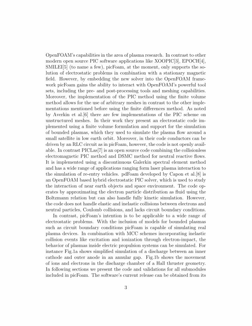
In general, simulations conducted with picFoam follow the PIC-MCC schemedepicted in Fig.2. Here the classic scheme[10] including Monte Carlo Colli-sions is drawn using boxes with rounded off edges, additional steps taken bypicFoam during a time step are drawn using boxes with sharp edges.

Figure 2: Particle-in-Cell scheme. The classic computation cycle[10] is depicted usingboxes with rounded off edges, additional boxes show further steps performed by picFoam.

The simulation process can be summarized as follow. First, precedinga simulation, an initialization step is performed by using the applicationpicInitialise, which is provided by the picFoam repository. With this pre-processing tool particles are distributed in the domain, an initial electric fieldE is solved, and models, selected by the user, are initialized as described insection 2.3.After the initialization, the simulation is run using the application picFoam.Every time step the scheme processes the following steps until the end timeis reached.

Step 1: Injection of new particles from boundaries. picFoam supportsvarious boundary and emission models as will be discussed in section2.7.

Step 2.1: Integration of the velocities of all particles using the leapfrogscheme and the various integration algorithms (see section 2.4).

Step 2.2: Moving all particles with their updated velocities usingOpenFOAM’s barycentric particle tracking (see section 2.4.1).

Step 3: Performing Monte Carlo Collisions, this includes models forbinary collisions between neutral species and Coulomb collisions of

5

charged particles (see section 2.8).

Step 4: Weighting the charges of all particles to the mesh as will bedescribed in section 2.5.

Step 5: Integration of the field equation Eq.1 using the finite volumemethod and OpenFOAM’s matrix solvers.

Step 6: Weighting the electric field to the particle position (see section2.5), which in turn is used to integrate the equation of motion in step2.1.

Step 7: Calculation of diagnostics as will be described in section 2.9.

Each procedural step is implemented in a modular way using submoduleclasses, which rely heavily on the template programming techniques used byOpenFOAM and allows for the selection of the various models at run time.

Figure 3: Schematic structure of a picFoam simulation case.

2.2. Case structure

Simulations conducted with picFoam are set up using OpenFOAM casestructure consisting of time directories, a constant, and a system directory.The time directories contain the fields calculated by the solver at differenttime points. Simulations start from initial fields in the ”0” time directory,here boundary conditions for the electrostatic potential field phiE need tobe supplied by the user as well.The constant directory containing the numerical mesh in a subdirectorycalled polyMesh and constant settings concerning the simulation in the dic-tionary file picProperties. Meshes can be generated with OpenFOAM’s

6

meshing utilities foremost blockMesh and snappyHexMesh, however, the im-porting of several popular mesh formats from other meshing utilities andconversion to OpenFOAM’s own format is also supported.In the picProperties dictionary the user sets physical properties of the con-sidered species and selects models for all submodules, for more details thereader is referred to the corresponding sections of this paper.The system directory includes parameter settings for the solution proce-dure, within this directory three files are required for the functionality ofOpenFOAM: the controlDict, which controls time and solution output,fvSchemes, which controls the schemes used in discretization process, andfvSolution, which determines the matrix solver used. Additional files forcontrolling the utilities provided by OpenFOAM, e.g. the decomposition inparallel processing are also supplied in the system directory.

2.3. Initialization

To initialize a simulation case the picFoam repository includes picIni-tialise, a pre-processing tool used to distribute particles in the domain andinitialize the submodules of the solver. It is build on the same principle asits main application using submodules to make it easy for a user to extendits features.For the initialization process the user supplies macroscopic quantities liketemperatures and number densities for each species, and picks an initializa-tion model in the [case]/system/picInitialiseDict dictionary. By defaultpicInitialise provides a number of different initialization models. These mod-els include, listing only a few, an equipartioned distribution of particles fromMaxwell-Boltzmann distribution, a quasi-neutral initialization of plasma, aninitialization from a list, where positions and velocities of single particles canbe supplied, or a model for a uniform distribution of particles. If not requiredby the initialization model for the distribution of particles, picInitialise au-tomatically calculates the number densities and temperatures for all species.After the distribution of the particles, the application initializes the collisionmodels used by picFoam (see section 2.8) and solves the initial electric field,which is used to prepare the particles for the leapfrog scheme (see section2.4).In the final step the application performs initial checks on restrictions setby the PIC method. These include a special restriction, as shown by C.K.Birdsall [11], where the cell dimensions need to be in the order of the Debyelength

7

λD =

√ε0kB/e2

ne/Te +∑

j Z2j nj/Ti

, (2)

to suppress the growth of nonphysical instability. In this context the Debyelength describes a shielding effect of the electrostatic potential of a chargetrough the self arranging of charges with different sign around the particleconsidered[12]. Here ε0 = 8.854... · 10−12 As/Vm is the vacuum permittivity,kB = 1.380... · 10−23 J/K is Boltzmann’s constant, e = 1.602... · 10−19 As isthe elementary charge, Z indicates the charge number of the ionic species j,n represents the number densities and T are the species temperatures. Thesecond restriction owed to the particle pusher, is different for all pushers,however a general stability criterion linked to the explicit leapfrog scheme,used in picFoam, can be formulated [13]. Revealing that the time step hasto be smaller than twice the plasma frequency

ωpe =

√ne e2

ε0me

. (3)

The parameter in Eq.3 have the same meaning as before, additionally, me =9.109... · 10−31 kg is the rest mass of an electron. The plasma frequencydescribes the oscillation of electrons around positively charged ions, due tothe attractive Coulomb forces and the inertia of the electrons, causing themto pass the equilibrium position[12]. Further monitoring of plasma frequencyand Debye length during simulation with picFoam can be turned on in thedictionary [case]/constant/picProperties.For statistical accuracy a high enough number of particles per cell is needed,to ensure this, picInitialise prints statistics on the cell occupancy along withother statistics like particle velocities, number densities and temperatures forall species, after the initialization.

2.4. Particle pusher

Commonly in the PIC method the leapfrog scheme[14] is used for theintegration of the particle’s equation of motion. In this scheme the averagevelocity existing at time tn+1/2 is used to move the particle forward. Toachieve this, the initial velocity of the particles is set back by half a timestep during the initialization. Doing so the velocity and position of a particleare not known at the same time, but leap over each other during simulation

8

Figure 4: Leapfrog scheme. Initially the velocities of the particles are set back by half atime step, resulting in the temporal leap frogging of spatial and velocity data.

(see Fig.4).To perform the velocity integration on every particle in the electromagneticfield (picFoam supports the use of a constant magnetic field), the PIC methodapplies the Lorentz force FL to compute a new velocity for each particle.

mdγu

dt= FL = q(E + u×B) (4)

In Eq.4 the vectors for the electric E and magnetic B field are known at in-tegral time steps, while the velocity u is known at half integer time steps. In

this equation the parameter γ =√

1 + |u|2 /c2 represents the Lorentz factor.

To solve Eq.4 various models are implemented, these include the relativisticmodels of Vay[15], Higuera and Cary[16], and the commonly used model ofBoris[17] in non-relativistic and relativistic form. The model is chosen by set-ting the ParticlePusher entry in the file [case]/constant/picProperties.

2.4.1. Barycentric particle tracking

To move the particles through the domain, picFoam uses OpenFOAM’sbarycentric particle tracking. This allows for tracking which is defined interms of displacement, without any search or correction algorithm. It leadsto advantages in the linear weighting algorithm (see section 2.5), and theboundary treatment. In the following paragraph we explain the fundamentalsteps of this algorithm for a stationary mesh.Each arbitrarily polyhedral cell in an unstructured finite volume mesh can bedecomposed into tetrahedra, these are constructed by triangles on the cell’sfaces and the cell’s center point (see Fig.5). The tetrahedra are then used todefine the position of each particle in terms of topology of the tetrahedronand the place of the particle inside it, specified by barycentric coordinates.

9

.

Figure 5: Illustration of one tetrahedron in the cell decomposition of hexagonal cell andof the barycentric description of a particles position.

These coordinates y define the Cartesian position x as a weight of the sumof the tetrahedron’s vertices a,b, c,d

x = ay1 + by2 + cy3 + dy4. (5)

Transformation from the Cartesian to the barycentric coordinates are per-formed using the transformation tensor A constructed from the tetrahedron’sedges

A · y = x− a, (6)

where the tensor

A = [−→ab,−→ac,−→ad]. (7)

A search of the particle’s position in the mesh and calculation of the barycen-tric coordinates is only required once when introducing a new particle intothe domain, as barycentric coordinates are handled as primary data and areautomatically updated while tracking the particle.The tracking works by moving from tetrahedron to tetrahedron, interactingwith all cell faces hit on the way. The linear change of a particle position inCartesian coordinates is found using

xnew = x + λxd, (8)

where xd = (1−f)u∆t is the particle’s global displacement, with f as the stepfraction keeping track of the already covered global track and λ the fractionof the current track to the next face. For more details on the Cartesianparticle tracking in older OpenFOAM versions correspond to Macpherson etal.[18].Using the inverse transformation tensor

10

T = det(A)A−1

(9)

and

µ =λ

det(A)(10)

Eq.8 is transferred to an update of the barycentric coordinates of the particle

ynew = y + µT · xd. (11)

Hits with the triangle faces of the tetrahedron are found by setting (ynew)i =0 and solving for the smallest

µi = − yi

(T · xd)i. (12)

Doing this means that there is no division by det(A) anywhere in the al-gorithm allowing it to function on inverted or degenerate tetrahedra. Theresulting µ is then used to update the particle’s coordinates using Eq.11 andthe step fraction f using det(A)µ. Following this a check if µ is greater thandet(A) reveals if the track of the particle ends in the current tetrahedron. Ifthis is the case, the overall track of the particle is finished, else the hit trian-gle face of the tetrahedron is checked for a number of cases before continuingthe track with the updated step fraction. In the first case, if the triangle doesnot belong to a cell surface, the particle switches to the adjacent tetrahedronin the current cell and continues its track. If the particle hits a cell surfaceneighboring another cell, the particle switches to the other cell updating itscell occupancy. If the cell face belongs to an boundary, immediate interac-tion with the boundary model is possible resulting in a reflection, deletion ormore complex interactions.Using this barycentric tracking algorithm the particle’s location is alwaysknown and the need for a computational expensive mesh searching algorithmafter each particle movement is avoided. When compared to other equivalentCartesian algorithms, the barycentric condition (ynew)i = 0 of finding the in-tersecting triangle on the particle’s trajectory is exact, preventing round offerrors, associated to the determination of the hit triangle face in other algo-rithms. This means tracking errors where the particles can get ”lost” when

11

hitting the triangles vertices or edges are avoided. For further implementa-tion details of the algorithm correspond to OpenFOAM’s software repository[19].

2.5. Weighting

In order to calculate the forces acting on the particle self-consistently,picFoam has to calculate the charge density, solve the electrostatic Poissonequation and obtain the electric field, which is, in the electrostatic case, thenegative gradient of the potential field E = −∇φ. These steps require twointerpolations also called weighting. First, the particle’s charge is weightedfrom its position to the numerical mesh and second, the field is weightedback from the electric field, defined on the mesh, to the particle’s position[10]. picFoam supports two methods which can be selected at run time inthe SolverSettings dictionary in [case]/constant/picProperties.

2.5.1. Cell average weighting

The simplest method sums the charges Q = ωpqp of every particle N ip to

their corresponding cell indicated by the superscript i and divides by the cellvolume to obtain the charge density field. Since this method directly assignsthe charge to each element and divides by the volume, charge is guaranteedto be conserved.

ρic =1

V ic

Npi∑

j

Qj (13)

After solving the Poisson equation, the electric field vector of a cell is usedon every particle in its corresponding cell to calculate the force acting on it.The cell average method is very fast, since only a summation of the chargesis necessary for all cells. The disadvantage of this method are the relativelynoisy fields, and therefore high gradients between neighboring cells.

2.5.2. Volume weighting method

The second weighting method implemented in picFoam uses the barycen-tric coordinates, that are known for all particles at any point in time (seesection 2.4.1). This allows picFoam to effectively calculate the weighting ofthe charges to surrounding cells. The following paragraph describes the im-plemented method.Barycentric coordinates are equivalent to the ratios of the sub tetrahedron’s

12

volume Vi, constructed with position x of the particle, and the volume Vt ofthe entire tetrahedron the particle is located in[20]. Using these coordinates,charge is weighted to the vertices of the cell using

Qk =

Npi∑

j

Qj ck, (14)

where k = 2, 3, 4 denote the vertices of the tetrahedron that coincide withvertices of the cell. The weighted amount of charge Qk for k = 1 is assignedto the cell’s center, since the sum of the barycentric coordinates

∑i ci = 1,

charge is conserved and errors only occur in the order of magnitude of thecomputational accuracy, as for the cell average method. In the next step,after communicating the charges on the vertices over processor boundariesand accounting for periodic boundary conditions, the summed charges aredistributed back from the vertices to all adjacent cells. Hereby the distancefrom the vertex to the cell center divided by the sum of the distances to allcell centers, surrounded by the respective vertex, is used. On the cell centeredfield, the interpolated charges are added to the value Q1 and a subsequentdivision by the cell volume Vc leads to the charge density ρic, which is usedby the field solver.After the new electric field has been computed, it has to be weighted backfrom the cell-centered field to the particle’s position. Hereby the field vec-tors are interpolated from the cell center to all vertices using the distances tothem. Again, after communicating over processor boundaries and accountingfor periodic boundary conditions, the barycentric coordinates of the parti-cles are used to linearly interpolate the electric field to the position of theparticles.This weighting method has a higher computational cost, when compared tothe cell averaging method, but leads to much less noisy fields, which can re-sult in more exact solutions, when compared to the first method (see section3.2).

2.6. Maxwell solver

Currently, picFoam only supports the solution of the electrostatic Poissonequation Eq.1. Like for every other submodule in picFoam, the selection ofthe model can be done at run time setting the MaxwellSolver entry in the[case]/constant/picProperties dictionary, hereby giving the user the op-tion to choose between no solver and the electrostatic solver. Settings for the

13

discretization process of the finite volume method and the matrix solver arespecified in the [case]/system/fvSchemes and [case]/system/fvSolutiondirectories respectively.

2.7. Boundary models

Within picFoam there is a variety of boundary models to choose from.Their selection is done in the [case]/constant/picProperties sub dictio-nary BoundaryModels.There are two base models, which have to be selected, the first specifies thereflective interaction from wall boundaries by setting the WallReflection-Model entry. Here picFoam supports simple specular reflection and morerealistic diffusive reflection models dependent on the temperature of the wall.The implementation of these models is borrowed from OpenFOAM’s DSMCsolver.The second base model defines the boundary condition and interaction withsimple patch boundaries, comprised of all boundaries, that are no wall orspecial boundary like periodic or symmetry boundary conditions. Patchesdefined by this second base model can represent an open boundary like a freestream boundary implemented similar to the model used in OpenFOAM’sDSMC solver or a simple injection model, that emits particles from theboundary according to a supplied injection frequency and velocity model.The models are selected by specifying patch names and the assigned modelin the PatchBoundaryModels sub dictionary. In this, picFoam allows forthe selection of different boundary models on different patches other thanOpenFOAM’s DSMC solver. Another class of important boundary modelsimplemented within picFoam are circuit models based on the work of Ver-boncoeur et al.[21] (see section 2.7.1).In addition to the two base models, picFoam also includes so called eventmodels, which can be used additionally to the base models on all bound-aries. Their main purpose is to perform diagnostic calculations like deletionstatistics, but they also include sputtering models which can be used on e.g.wall boundaries. Patch event models are selected through the PatchEvent-Models dictionary entry.

2.7.1. Circuit boundary models

The addition of circuit boundary models allows picFoam to analyze boundedplasmas. Implemented are simple open circuit and general purpose circuitmodels consisting of a resistance, an impedance, and a capacity in series (see

14

.

Figure 6: Scheme of a bounded plasma with external RLC circuit in one dimension.

Fig.6). The open circuit models include a floating boundary model, a shortcircuit ideal voltage, and an ideal current source model. The usage of thesemodels requires boundary conditions joining the circuit charge to the plasmadomain, these are based on Gauss’ law Eq.15 using the surface charge σ andapplying it to the boundary surface of finite volume mesh.

∮

S

εE · dS =

∫

V

ρc dV +

∮

S

σ dS = Q (15)

In electrostatic problems solving the Poisson equation, the relationship

E = −∇φ =σ

ε(16)

is used to specify the surface charge σ as a gradient boundary condition forthe electrostatic potential. As shown by Vahedi et al.[22], the time variationof the surface charge, may be obtained from Kirchhoff’s current loop law

dσ

dt= Jconv +

I(t)

A, (17)

where I(t) is the external circuit current, A the area of the boundary repre-senting the electrode, and Jconv is the convective current density supplied tothe electrode by charged particles. The discrete finite differenced form is

A(σt − σt−1) = Qt −Qt−1 +Qtconv, (18)

15

where Q =∫dtI is charge deposited by the external circuit current. The

conservation of charge Eq.18 is used to update the surface charge every timestep. Using the general circuit, consisting of a resistance R, an impedance L,and a capacity C in series, the charge Q existing in the capacitor is advancedusing Kirchhoff’s voltage law

Ld2Q

dt2+R

dQ

dt+Q

C= V (t) + Φa − Φc. (19)

In the implementation of picFoam, Φc is the potential averaged at the drivenboundary, while Φa acts as the reference potential for the system and is fixedto zero at the second boundary.Eq.19 is differenced using the second-order backward Euler representation asdescribed by Verboncoeur et al.[21] and transformed into a gradient boundarycondition using Eq.16 and Eq.18.

∇φ =φtb − φtc

∆x=

1

α0ε0A+ ∆x

(−φtc+α0Aσ

t−1+α0(Qtconv−Qt−1)+(V (t)−Kt)

)

(20)Eq.20 specifies the potential gradient between the boundary φtb and the

value at the cell center φtc at time t. ∆x is the distance between the cellcenter and the boundary face and A is the area of the boundary surface,while α0 and Kt have the same definition as in Verboncoeur et al.[21].

Kt = α1Qt−∆t + α2Q

t−2∆t + α3Qt−3∆tα4Q

t−4∆t

α0 =9

4

L

∆t2+

3

2

R

∆t+

1

C

α1 = −6L

∆t2− 2

R

∆t

α2 =11

2

L

∆t2+

1

2

R

∆t

α3 = −2L

∆t2

α4 =1

4

L

∆t2

(21)

When an open circuit is used, the gradient boundary condition simplifiesto Eq.16. In the case of a floating boundary condition, where the impedance

16

approaches infinity, the second term in Eq.17 is ignored and the surfacecharge is modified through the plasma convection current Jconv only. Anideal voltage source reduces to a specified potential difference between thetwo electrodes

φa − φc = V (t). (22)

The last open circuit boundary model is a current driven external circuit,where assuming an ideal current source, the surface charge is driven by ap-plying the time-varying current I(t) (see Eq.17), other circuit elements areignored [21].The emission of electrons from the boundary is controlled by the Emission-Model integrated into all circuit boundary models. Models are selected byspecifying the model name in the EmissionModels list, contained withinthe [case]/constant/picProperties boundary model dictionary. Multiplemodels can operate simultaneously. Implemented are thermionic emissionfor a given temperature according to Richardson’s law[23] and field electronemission based on the work of Fowler and Nordheim[24].A third model performs emission through sputtering of electrons by impact ofheavy species, implemented similar to the BoundaryEvent sputtering model.In both implementations the user specifies the probability for the emissionof selected species by impact of other species and the energy of the newlycreated species.All emission models inject uniformly from the surface of the selected bound-ary patch, the models maintain this uniform distribution on separated sur-faces that may occur in parallel simulations. For emission caused by speciesimpact using the sputtering model, which occurs during the movement of theparticles (see section 2.4), the model automatically corrects the velocity of theparticle and moves the new particle the remaining fraction of the time step.Velocities for injected particles are sampled from inverse Maxwell-Boltzmanndistribution [10].

2.8. Collisions

Plasmas which are simulated with the classic PIC scheme are collisionless,this means that forces acting on the individual particles are only a source oftheir macroscopic fields. As a consequence, fields generated by individual par-ticles are excluded, meaning the field decreases with decreasing distance, andinter-particle forces inside a mesh cell are underestimated. To compensate

17

this error picFoam implements a Coulomb collision submodule as discussedin section 2.8.1. In addition to this, picFoam also performs binary collisionsbetween neutral species in order to account for inter-molecular forces, as wellas collisions between heavy ion and neutral species, both managed in a sepa-rate submodule (see section 2.8.2). A third collision submodule handles thecollisions between electrons and neutral species, this submodule includes avariety of collision events and corresponding cross section models (see section2.8.3).Besides the simulation with discrete neutral particles, picFoam also supportsthe simulation with a background gas model. This model is used for simula-tions where the neutral gas density is much higher than the plasma density,freeing memory by removing the need of simulating a lot of numeric par-ticles and thereby greatly reducing the overall computational cost. In thismodel velocities of neutral particles, used in the collision process with otherspecies, are sampled based on the Maxwell-Boltzmann distribution, using abackground density and a temperature field. The background model is fullyincorporated into the collision algorithms, meaning that in addition to thebackground models, neutral particles can be simulated at the same time, ifrequired. All submodules mentioned are selected at run time in the Colli-sionModels dictionary in [case]/constant/picProperties.The calculation of the new velocities while scattering are based on the as-sumption of equal particle weight. Since picFoam supports arbitrary weightedparticles, meaning one simulated particle includes a arbitrary number of realparticles, a correction has to be performed. If this correction step is neglectedin the collision between particles whose weights are different, the particle withthe higher weight would be scattered too much, resulting in a artificial heat-ing of the system. For the correction, two models have been implemented.In the simplest model, described by Nanbu and Yonemura[25], the particlewith the higher weight only undergoes a collision with a probability of theratio of the lower to the higher weight. Since this method does not conserveenergy and momentum in every collision, it only works well in the case ofhigh particle numbers. The second model implemented, described by Sen-toku and Kemp[26], does not have this limitation, here the heavier particle’svelocity is reduced in way that energy and momentum are conserved.

2.8.1. Coulomb collisions

The Coulomb collision algorithms implemented in picFoam are based onthe binary collision model introduced by Takizuka and Abe [27]. In this

18

model charged particles in a cell are paired randomly with another chargedparticle for collision. The idea behind this is that the long-ranged Coulombcollisions between two charged particles are negligible on distances higherthan the Debye length. Which can be done because in the PIC method cellsizes are typically in the order of this length.The original implementation of Takizuka’s and Abe’s model is only valid forcharged species whose weight is equal among all particles of one species, forthis reason picFoam also implements the model of Nanbu and Yonemura[25]for pairing arbitrary weighted particles. Due to these models purpose of pair-ing charged particles, they are called PairingAlgorithm within in the con-text of the solver, which can be selected in the [case]/constant/picPropertiesdictionary. This PairingAlgorithm represents one part of the Coulombcollision algorithm, the second model specifies the calculation of the particlescattering process. Implemented is a model based on the work of Nanbu[28].In it the collisions are handled in a cumulative way; a succession of small-angle collisions is grouped into a unique large scattering angle collision, mak-ing it possible to treat the collision like one between neutral atoms. Fullyrelativistic collisions are also implemented based on the work of Perez etal.[29]. Moreover, the solver implements the collisional ionization model forion species described by Perez et al.[29], which can be used in combinationwith both Coulomb collision models mentioned here. This model calculatesan ionization cross section based on the atomic orbital binding energy, sup-plied by the user in the picProperties dictionary. Values for this can befound in references [30, 31]. An important measure in the Coulomb colli-sion is the dimensionless Coulomb logarithm. It can be seen as the ratioof the probabilities for large-angle scattering through successive small-anglecollisions over a large-angle scattering through a single Coulomb collision.It is an important parameter in the calculation of the deflection angle. Bydefault the value of the Coulomb logarithm is calculated during collision,however, with picFoam the value can also be set to any user defined valuefor all different collision partners.

2.8.2. Binary collisions

Binary collisions between neutral species and neutral-ion species are im-plemented based on the Null-Collision method developed for simulation ofrarefied gases using the Direct Simulation Monte Carlo(DSMC) method de-scribed by Bird[32]. The collisional interaction between these species is shortranged and the scattering is treated as isotropic. In our implementation,

19

collision probabilities are determined from a total cross section model usingthe hard-sphere model as approximation. For some simulations like DC dis-charges, where ions with high kinetic energy in the plasma sheath can beconverted into ions with thermal energy in a charge exchange collision[33],we implemented the simple charge exchange model for inert gases describedby Nanbu and Wakayama[34]. In this model the cross section of the eventis expressed by half the total cross section calculated with the hard-spheremodel using a slightly higher, experimental validated, particle diameter.

2.8.3. Electron neutral collisions

The last collision submodule handles collisions between electron and neu-tral species. Implemented are elastic, inelastic excitation, and ionizationcollisions, all based on one collision algorithm. In this model scattering isdependent only on electron energy, for low energies scattering is isotropic,while with increasing energies scattering takes a form of forward scattering.In inelastic collision events, precollision velocities are modified based on thethreshold energy of the specific collision event, making it possible to use onlyone algorithm. The validity of this method and implementation details arediscussed in Nanbu’s work[33].The selection of the collision event is done with the help of the Null-Collisionmethod, where the collision probability is calculated using the maximal pos-sible collision cross section σmax. In this method the collision is treated asreal with a probability equal to the ratio of the probability of the single event

Pc = ng |u|σ∆t, (23)

to the maximum probability Pc/(Pc)max or as not occurring with a probabilityof 1−Pc/(Pc)max. In Eq.23, ng is the number density of the gas the electroncollides with, |u| is its velocity and σ is the cross section for the specificevent. In the calculation of (Pc)max the variable σ is the maximal possiblecross section σmax. Several cross section models for the different collisionevents are implemented[35, 36, 37, 38], which can be independently selectedin the sub dictionary CrossSectionModels in the settings dictionary of theelectron neutral collision model.

2.9. Diagnostics

The diagnostics submodule provides a number of models printing infor-mation on species to the standard output at run time. These models include,

20

among others, diagnostics information on temperature, kinetic and potentialfield energy, momentum, and the composition of the particle cloud. Infor-mation are printed as global averages and for separate species. The selec-tion of independent models takes place in the sub dictionary Diagnosticsin [case]/constant/picProperties, optionally for every model calculationtime points can be specified here, reducing the computational costs.

3. Validation

In this section validations for the different submodules are presented.

3.1. Particle pusher

The first validations are simple simulations that look at the movementof a single particle in constant electric and magnetic fields separately. Afterthat, a more elaborated test looks at the plasma oscillation of a plasma,which validates the particle pusher and Maxwell solvers cooperative work.

3.1.1. Electrostatic acceleration

In this test a single electron particle is accelerated through constant elec-tric fields calculated from fixed potential differences in a 1D mesh.From energy conservation Eq.24 we retrieve the final velocity after a chargehas passed through the potential difference. In this relation m = γme is therelativistic mass with rest mass me of the electron. v is the magnitude of theparticle’s velocity, q is its electric charge, and U is the potential differencethe particle is accelerated through.

Ekin =1

2m |u|2 = qpU = Epot

→ u =

√2qpU

m

(24)

For this test we initialize the electric field without space charge, after thatan electron is created with zero velocity at the left boundary of the 1D mesh.During the simulation the Maxwell solver is turned off, since the space chargewould significantly alter the electric field on simulations with low potentialdifferences. The mesh dimensions and cell division are irrelevant, given thatthe Maxwell solver calculates the correct electric field strength, the particle’sfinal velocity has to coincide with the theoretical value of Eq.24.

21

0

0.2

0.4

0.6

0.8

1

10610 100 1000 10000 100000

|~v|/c

0[-]

potential [V ]

theoryBorisVay

Higuera&Cary

Figure 7: Final velocity of an electron accelerated through various potential differences.

As can be seen in Fig.7 the final velocity matches the theoretical curve forall simulated potential difference.

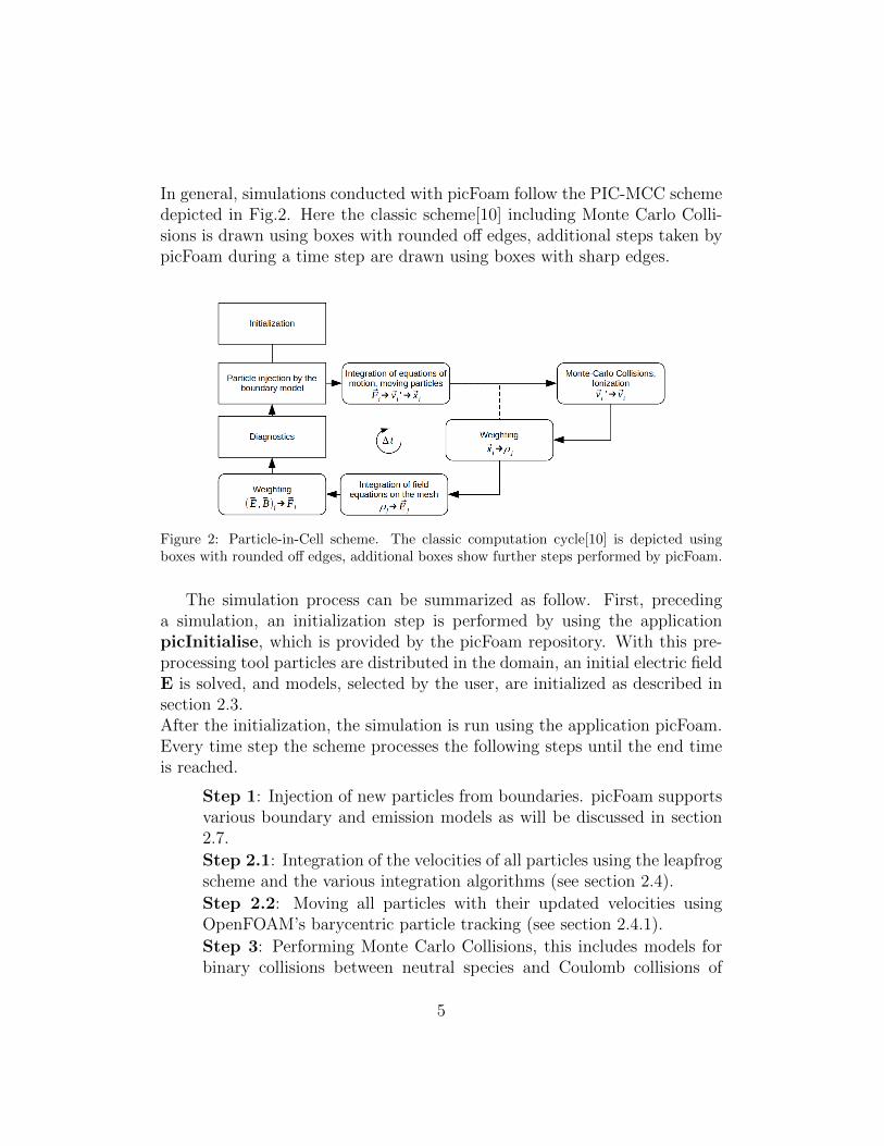
3.1.2. Rotation in magnetic field

Here we validate the implementation of the magnetic rotation of all mod-els. To do so we compare the circular trajectory of a single electron ina constant magnetic field to its theoretical circular trajectory with the ra-dius of gyration given by rg = mu⊥/ |qp| B. A single electron is placed atx = (0,−rg, 0)T with a velocity of u⊥ = 0.1c0 in a 2D rectangular mesh of400× 400 mm2 with 40 cells in every valid dimension. The Maxwell solver isturned off during the simulation, the time step is set to 0.1 fs and the simu-lation ends after 1000 rotations. The magnetic field Bz = 1 T is constant.Fig.8a shows the final trajectory after 1000 loops and its agreement withtheory. To explain the deviation of Higuera and Cary’s model from the othertwo, we conducted a analysis of the angular frequency ωl = |qp| B/m. Forthis we compute the Fourier transformation of the particle’s x-coordinate intime. Fig.8b shows the power spectra of the Fourier transformation. Thepeak for Boris and Vay’s method is at 27.85 GHz, giving an error below 1%to the theoretical value of 28 GHz. Note that the sample frequencies are mul-tiple of 25 MHz. For Higuera and Cary’s method the Fourier analysis showsa peak at 27.925 GHz giving a smaller error than Boris and Vay’s methods,this showing that all methods implemented are in very good agreement with

22

−1

−0.5

0

0.5

1

−1 −0.5 0 0.5 1

posi

tion

y/r

g[-]

position x/rg [-]

theoryBorisVay

Higuera&Cary

(a) Trajectory of an electron after completing 1000loops in a constant magnetic field Bz = 1 T.

(b) Power spectra of the Fourier transformation ofthe electron’s x-coordinate in time. The inner graphshows the zoom around the tips.

Figure 8: Results for the validation of section 3.1.2

theory.

3.2. Plasma oscillation

In this validation we look at the plasma oscillation of electron speciesdeflected from a uniform ion background, validating the particle movementin combination with the computation of the electric field. For this test 1.536million ion parcels with a weight of ωp = 2.5 · 106 are uniformly distributedin 6 m× 0.8 m× 0.8 m wide mesh with 120× 16× 16 cells. From the locationof the ion parcels the same number of electrons, deflected in the x-directionby ∆x = A sin(kx1) with an amplitude of A = 0.1 m and a wavenumberof k = 4π/6 m, is placed inside the mesh. This leads to a number densityof ne = 1013 m−3, according to theory[12] the electrons oscillated with anangular frequency of ωpe =

√nee2/(ε0me), where me is the rest mass of

an electron, giving us a period of T = 2π/ωpe = 35.22 ns. Initially, bothspecies are at rest, during the simulation the ion species is kept fixed, whilethe electron species starts oscillating accelerated by the potential gradientinduced by the deflection from its equilibrium position at the ions. Theemerging plasma frequency is determined from two periods of the total kinetic∑

0.5γme |u|2 and field energy∑

0.5ε0 |Ec|2 /Vc, due to the electron havingto pass the equilibrium position twice for a whole oscillation period [39].Here Vc is the cell volume and Ec is the electric field vector defined at thecell center.

23

0

1

2

3

0 20 40 60 80

35.17 ns 35.17 ns

Tot

alen

ergy

[mJ]

Time [ns]

kin. Epot. E

.

Figure 9: Plot of the particles total kinetic∑

0.5γme|u|2 and the corresponding electricfields total potential energy

∑0.5ε0|Ec|2/Vc over time. Two cycles through the equilib-

rium position correspond to the plasma frequency ωpe, with its period T = 2π/ωpe.

Fig.9 shows the energy plot over time. The evaluation of the results ispresented in Tbl.1, showing an error for the oscillation period below 1% forboth implemented weighting methods. The second and third row of the tableshow an evaluation of the energy conservation, here the error represents theaverage deviation from the first peak of potential and kinetic energy, reveal-ing that the volume weighting method (section 2.5.2) provides conservation ofenergy two orders of magnitude higher than the cell average method (section2.5.1). The last row shows the evaluation of momentum conservation, herewe look at the trend of the total momentum of the system in x-direction. Forthe simulation parameter mentioned above, leading to an average number ofNCP = 50 particles per cell per species and using the cell average method we

observe an unstable behavior. Which is further increasing over time due tothe instabilities induced by noise in the charge density field. For the volumeweighting method a stable oscillation in the total momentum is observedwith an error of 2.8% per period of the plasma frequency. Increasing NC

P to100 reduces the error for the volume weighting method to 1.61%, while thebehavior using the cell average method stays unstable due to prevailing noise.

An accurate representation of the charge density field is an important fac-tor in the correct description of the plasma. In this, the weighting method

24

CellAverage VolumeWeighting

period T[ns] 35.01 35.17error [%] 0.59 0.14max Epot [mJ] 2.797 2.795error ∆Epot [%] 0.96 0.0065max Ekin [mJ] 2.797 2.788error ∆Ekin [%] 0.53 0.0057error ∆px [%] (NC

p = 50) – 2.82error ∆px [%] (NC

p = 100) – 1.61

Table 1: Computed period of the plasma oscillation using different weighting schemes andthe error to the theoretical value of T = 2π/ωpe = 35.22 ns. The second and third rowshow the energy conservation by the average deviation from the first peak of the totalkinetic and potential field energy at NC

P = 50. The last row shows the error per oscillationperiod in the momentum conservation for different number of particles per cell.

has a big impact on the noise of the field. Fig.10b shows the charge densityfield in the x-direction of the simulation with NC

P = 50. As can be seen, com-pared to the volume weighting method, the cell average method introducesslight noise to the field. To quantify the noise introduced by the differentmethods, we compare the initial fields calculated by both methods for differ-ent numbers of particles per cell in the range of 5 to 100 to the initial fieldproduced by the volume weighting method with 1000 particles per cell. Bycalculating the L2 norms of the relative errors we obtain an indication of theaccuracy of the weighting method. Fig.10a shows that the field calculatedwith 5 particles per cell and the volume weighting method is more accuratethan the field calculated for 100 particles per cell and the cell average method.Therefore, despite the higher numerical cost, it is recommended to use thevolume weighting method for simulations conducted with picFoam. Whileboth methods accurately conserve energy, the cell average method tends toinaccurately conserve momentum because of noise introduced to the chargedensity field. Over time this will lead to a loss of physical fidelity. Similarwas observed by Capon et al. [8], which implemented a cell average methodand a related volume weighting method and showed an inaccuracy in thevelocity of a single electron oscillating around an ion, when using the cellaverage method.

25

10−5

10−4

10−3

10−2

10−1

100

0 20 40 60 80 100

L 2

NP /cell

Cell AverageVolume Weighting

(a) L2 norm of the relative error in the charge den-sity field plotted over the number of particles NP

per cell.

−4 · 10−7

−2 · 10−7

0 · 100

2 · 10−7

4 · 10−7

0 1 2 3 4 5 6

Cha

rge

dens

ity[ A

sm

3

]

Length [m]

Cell AverageVolume Weighting

(b) Initial charge density over the domain lengthof the simulation in section 3.2 at NC

P = 50, hereshowing noise when using the cell average methodcompared to the volume weighting method.

Figure 10: Investigation of noise in the charge density field for the implemented weightingmethods.

3.3. Collision and Ionization

To validate the collision algorithms implemented in the new code, simula-tions are run in which two species are initialized with different temperaturesbut with no relative drift, in this case their equilibration is described by

dTαdt

=∑

β

ν α|β(Tβ − Tα). (25)

Where ν α|β is the mean collision frequency of species α with species β [40].

3.3.1. Neutral-Binary collisions

The first collision submodule handles collisions between neutral species aswell as collisions of neutral with ion species. The interaction is short range,we treat the collision by using the hard-sphere model. Scattering is isotropic.The mean collision frequency for species α with species β is described byν α|β = nβgσT , where g is the mean relative velocity, nβ the number densityof species β, and σT the hard-sphere cross section π(dα + dβ)2/4, which isconstant. For the validation of this submodule argon and neon atoms withan atomic mass of 39.948 u and 20.18 u, and van der Waals radii of 188 and154 pm are used. Particles are equably initialized with a number density of1022 m−3 respectively on a 15µm×15µm 2D mesh with a total of 64 cells.

26

500

600

700

800

900

1000

0 0.5 1 1.5 2

Tem

pera

ture

[K]

Time [µs]

∆W = 1∆W = 2∆W = 5

theory

.

Figure 11: Thermalisation of species argon and neon trough binary collisions, simu-lated with three particle weight differences using the correction scheme of Nanbu andYonemura[25].

Velocities are sampled from a Maxwell-Boltzmann distribution with argonbegin at 1000 K and neon at 500 K. Three simulations with weighting ratios(∆ωp = ωα/ωβ) of 1, 2, and 5 were performed, here the weight of ωα is keptconstant at 400. The correction method for differently weighted particlesdescribed by Nanbu and Yonemura is used [25].The theoretical collision fre-

quency is calculated with the mean relative velocity of g =√

8TkB/(µπ),

where T = T∞ = 750 K, and µ is the reduced mass of both species.Fig.11 shows the temperature profile, reasonable agreement with the theorywas achieved. Small deviations can be explained by the use of an meanrelative velocity g.

3.3.2. Coulomb collisions

This test uses the model described by Perez et al.[29] and is set up withthe same mesh as the validation in section 3.3.1. 160000 real electrons andargon ions are distributed in a way that each cell has the same number ofparticles so that the plasma is quasineutral with number densities of ne =ni ≈ 3.034 · 1022 m−3. Weight ratios are set to 1, 2, and 5 as before whilekeeping the weight of the ions constant at 400. The weighting correctionmethod used here is the model described in Sentoku and Kemp[26]. Forfaster convergence the mass ratio of the species ∆m = mi/me is set to 10,

27

10

11

12

13

14

15

16

17

18

19

20

0 0.5 1 1.5 2

Tem

pera

ture

[eV

]

Time [ns]

∆W = 1∆W = 2∆W = 5

theory

.

Figure 12: Thermalisation of electrons and argon ions trough relativistic Coulombcollisions[29], simulated with three particle weight differences using the correction schemeof Sentoku and Kemp[26].

where me remains constant at the rest mass of electron me = 9.109 · 10−31

kg.

ν α|β = 1.8× 10−19Z2αZ

2β ni√memi ln Λ

(meTe +miTi)3/2(26)

As in the last section the theory is described by Eq.25, this time using thecollision frequency stated by the NRL Plasma Formulary[40] shown in Eq.26.Initial temperatures are set to Te = 20 eV for the electrons and Ti = 10 eVfor the argon ions, the Coulomb logarithm is fixed to ln Λ = 15 for all possiblecollision partners. Fig.12 shows the temperature profiles over time and anexcellent agreement with the theory for all simulations.

3.3.3. Ionization

The last test for validation of the collision submodules looks at the ion-ization rate of a neutral argon species during electron impact. This allowsfor a validation independent of the other submodules as a thermalizationsimulation requires the other submodules for inter species collision.The same mesh and the three weight ratios as in the previous tests are used.Both species are initialized with a number density of 1022 m−3, the weightof the argon species is fixed at 100. Ionization is handled with a modeldescribed by Nanbu[33]. Since the ionization cross section is dependent on

28

0

0.2

0.4

0.6

0.8

1

0 0.2 0.4 0.6 0.8 1

Deg

ree

ofio

niza

tion

α[−

]

Time [ns]

∆W = 1∆W = 2∆W = 5

theory

.

Figure 13: Ionization of argon species in collision with electrons at a number density of1022 m−3 using a fixed cross section 3.5e−20 m2 corresponding to the initial electron energyof 100 eV.

the electron’s kinetic energy and this test aims to validate the algorithm, afixed cross section of 3.5e−20 m2 is used. This allows us to use Eq.25 for thedescription of the ionization, where instead of the temperature the numberof neutral and ion particles created are used. The ionization frequency isν α|β = nβgσi with g =

√8TekB/(meπ) the mean velocity calculated at the

initial electron temperature of 100 eV.Good agreement with theory can be observed in Fig.13. The deviation fromthe theoretical curve seen in all simulations here can be accounted to a chang-ing velocity distribution at later times.

3.4. Boundary model

3.4.1. Open circuit models

In this validation we look at the potential drop between a plasma anda collector represented by the floating boundary condition and compare itagainst theory. The open circuit boundary models, including the floatingpotential model, are implemented based on the gradient boundary conditionEq.16 and Eq.17, hence this test validates all implementations of open circuitmodels.Schwager et al.[41] derived two equations which together describe the sourcesheat potential drop ψp and collector potential ψc in terms of mass µ = me/mi

and temperature τ = Tsi/Tse ratios of the species, here ψ = eφ/Tse is the,

29

with the electron source temperature Tse, normalized potential. The firstequation is derived at the inflection point in the middle of the characteristiccurve, as can be seen in Fig.14, at this point ∆ψp = 0.

1√µτ

exp(−ψp

τ

)erfc(−ψp

τ

)1/2

= exp(ψp − ψc)[1 + erf(ψp − ψc)1/2] (27)

The second equation results from imposing the zero electric field conditionat the inflection point, written in separate terms of normalized integrateddensities ζ for electrons and ions.

ζi + ζe = 0 (28)

with

ζi =

√τ

µ

[exp(−ψp

τ

)erfc(−ψp

τ

)1/2

− 1 +(−4ψp

πτ

)1/2]

and

ζe = exp(ψp − ψc)[1 + erf(ψp − ψc)1/2]

+ (2/√π)(−ψc)1/2 − (2/

√π)(ψp − ψc)1/2

− exp(−ψc)[1 + erf(−ψc)1/2].

The simultaneous solutions of Eq.27 and Eq.28 exist in two points, one occursat dψc/dψp = 0, the other at ψp = 0. Here, the first solution is stable andrepresents the theoretical solution to the problem we compare to. For moredetails see Schwager et al.[41].Tbl.2 compares the theoretical solutions of µ = 1/40 and τ = 0.1, 1, and 5,to the solution of a one-dimensional simulation using the same parameter.Initially particles are distributed with a number density of n = 1018 m−3 inthe one-dimensional domain, which has a length of l = 132λD for τ = 0.1,l = 44λD for τ = 1, and 66λD for τ = 5, where λD is the correspondingDebye length. During simulation particles are injected from the source witha half Maxwell-Boltzmann distribution and a rate of 5.3 · 1012 Hz. Particlesreflected back to the source are re-injected with the source temperature. InTbl.2 the collector value has been read directly from the averaged field valueat the boundary, while the value for ψp has been averaged over the flat part

30

of the curve (see Fig.14). As can be seen, the error for the collector potentialis below 1% for all cases, only the ψp for τ = 5 shows a considerable error of10%.

Simulation Theoryτ\ψ ψp ψc ψp ψc

0.1 -0.7596 -1.532 -0.758 -1.5311 -0.278 -1.0389 -0.276 -1.0365 -0.0525 -0.487 -0.0582 -0.483

Table 2: Comparison of the simulated versus theoretical value of the potential at theinflection point ψp and the collector ψc at three different temperature ratios τ .

−1.8

−1.6

−1.4

−1.2

−1

−0.8

−0.6

−0.4

−0.2

0

0.2

0 0.2 0.4 0.6 0.8 1

Pot

enti

alΨ

[−]

Length xL [−]

τ = 0.1τ = 1τ = 5theory

Figure 14: Plot of the potential between the plasma source and the collector for all simu-lated cases (τ = 0.1, 1, 5). The crosses show the theoretical values calculated from Eq.27and Eq.28.

3.4.2. General RLC circuit model

For the validation of the RLC circuit boundary model, we perform twosimulations. First, we compare the current progression of an RLC circuitdriven by a sinusoidal voltage source over time with a theoretical solution.This validation is set up similar to the validation performed by Verboncoeuret al.[21]. In this simulation the plasma region is assigned to a permittivity of1020 with no plasma and the circuit elements are set to R = 1 Ω, L = 1µH and

31

C = 5µF. The voltage source follows the expression V (t) = V0 sin(ωt + θ),where V0 is set to 1 V, the angular frequency of 106 is used and the initialphase is set to zero. The time step is set to ∆t = 2π/128ω. As stated inVerboncoeur et al.[21] the theoretical solution can be predicted using

I(t) =a2V0/(ωZ) cos(θ − δ) + V0/Z sin(θ − δ)

a2/a1 − 1exp(a1t)

+a1V0/(ωZ) cos(θ − δ) + V0/Z sin(θ − δ)

a1/a2 − 1exp(a2t)

+V0

Zsin(ωt+ θ − δ),

(29)

where

Z =

√R2 +

(ωL− 1

ωC

)2

,

δ = asin(ωL− 1/(ωC)

Z

), and

a1,2 = − R

2L±√

R2

4L2− 1

LC.

Fig.15 shows the current plot over time up to t = 256∆t. As shownhere, the solution calculated by picFoam coincides with the one of PDP1in Verboncoeur et al.[21], and both agree well to the theoretical solution ofEq.29.

The second test looks at the evolution of current and voltage at the circuitdriven boundary over time. Compared to the first validation, the 1D domainof 5 mm × 2.4 mm × 2.4 mm set up with 200 cells, is filled with an argonplasma of density ne = ni = 1015 m−3, where the subscript indicates theelectron and ion species respectively. The species are initialized in thermalequilibrium using a Maxwell-Boltzmann distribution and a temperature ofT = 1 eV. Collisions between species are disabled and the circuit elementsare set to R = 1 Ω, L = 0.04 H and C = 1µF. The solution of the plasmainfluenced circuit behavior is compared to a simulation with XPDP1[21] usingthe same parameter as in picFoam. Fig.16 shows the voltage plotted overthe current for both codes, here showing good agreement between these twoimplementations with a mean error of 3% for the measured current.

32

−1

−0.5

0

0.5

1

0 2 4 6 8 10 12

curr

ent

[A]

time [µs]

theorypicFoamXPDP1

.

Figure 15: Comparison of the theoretical progression of current Eq.29 in an RLC circuitwith R = 1 Ω, L = 1µH and C = 5µF to the boundary model implementations in picFoamand PDP1 with no plasma and a permittivity of ε = 1020.

−50

0

50

100

150

200

250

−0.2 0 0.2 0.4 0.6 0.8 1

volt

age

[V]

current [mA]

picFoamXPDP1

.

Figure 16: Behavior of an RLC circuit with R = 1 Ω, L = 0.04 H and C = 1µF interactingwith an argon plasma of density ne = ni = 1015 m−3; comparison between XPDP1 andpicFoam.

4. Discussion

In this work we have presented the implementation and validation of pic-Foam, a fully kinetic electrostatic solver implementing the Particle-in-Cell

33

method including Monte Carlo Collisions for plasma research. The solveris developed in OpenFOAM building upon a robust particle tracking algo-rithm and the finite volume method. picFoam incorporates the same object-oriented design as the OpenFOAM toolbox, which makes it highly flexible bybeing able to select the different implemented models at run time and easyto extend because of the modular design, using C++ template programmingtechniques. picFoam implements state of the art models for all of its sub-modules, this includes particle collisions both relativistic and non-relativisticamong particles whose weights are arbitrary and defined on a particle toparticle basis. OpenFOAM’s novel barycentric particle tracking algorithmenables picFoam to efficiently manage the linear interpolation of the chargeand field weighting from and to meshes, on one to three spacial dimensions.Moreover, its application of general circuit boundary models allows picFoamto simulate real plasma devices.Validations for all implemented submodules have been presented, demon-strating picFoam’s ability to reproduce plasma phenomena. In section 3.1and 3.2 we have shown fundamental validations for the PIC method. In thesesimulations we checked the integration of motion by comparing the motionof charged particles against theory, here validating the consensus of theoryand simulation, since errors are far bellow 1% for all conducted tests. Thesimulation of plasma oscillation has shown excellent results for the imple-mented volume weighting method, which in comparison to the cell averagemethod introduces far less numerical noise to the simulation. By employingbarycentric particle tracking a novel approach of charge and field weight-ing for mesh based PIC methods without computational expensive particlesearch algorithms has been presented. Simulations for the implemented colli-sion algorithms have been shown in section 3.3, all algorithms were validatedindependently, overall conforming their correct implementation. Simulationsin this section were run using three different ratios of particle weights, thisalso validating the correction algorithms needed for the collision of arbi-trarily weighted particles. Small deviations from theory, seen here duringsimulations, can be accounted to the assumptions of a Maxwell-Boltzmanndistribution incorporated into the theories. Boundary models are validatedin section 3.4, here results obtained by picFoam agree with theory as well aswith results achieved with other solvers.The intention of picFoam is to be a useful platform for plasma research, it iseasy to set up new simulation cases by employing OpenFOAM’s strait for-ward case structure, as well as easy to extend through its modular design.

34

The development of picFoam is an ongoing process adding new features andbug fixes to its open source repository. Future efforts in extending picFoam’sfeatures include adding load balancing and the coupling to OpenFOAM’spowerful field solver capabilities. This coupling of fluid and Lagrangian de-scription would allow picFoam the simulation of individual species as fluidand thereby gaining the ability of conducting higher performing hybrid sim-ulations. Additionally, in the context of noise introduced by the weightingmethods (see section 3.2), the addition of filtering algorithm, as mentionedin Jacobs et al.[42], poses the opportunity for extending picFoam, therebyincreasing the robustness of the code.

Acknowledgments

We thank the DFG Deutsche Forschungsgemeinschaft (German ResearchFoundation) for funding this project under grant GR 2720/8-1. We alsolike to thank Will Bainbridge (CFD Direct) for his help in understandingOpenFOAM’s barycentric particle tracking.

References

[1] J. P. Verboncoeur, Particle simulation of plasmas: review and advances,Plasma Physics and Controlled Fusion 47 (5A) (2005) A231–A260. doi:10.1088/0741-3335/47/5a/017.

[2] H. Weller, G. Tabor, H. Jasak, C. Fureby, A tensorial approach tocomputational continuum mechanics using object orientated techniques,Computers in Physics 12 (1998) 620–631. doi:10.1063/1.168744.

[3] J. Verboncoeur, A. Langdon, N. Gladd, An object-oriented electromag-netic pic code, Computer Physics Communications 87 (1) (1995) 199–211, particle Simulation Methods. doi:https://doi.org/10.1016/

0010-4655(94)00173-Y.

[4] T. D. Arber, K. Bennett, C. S. Brady, A. Lawrence-Douglas, M. G.Ramsay, N. J. Sircombe, P. Gillies, R. G. Evans, H. Schmitz, A. R. Bell,C. P. Ridgers, Contemporary particle-in-cell approach to laser-plasmamodelling, Plasma Physics and Controlled Fusion 57 (11) (2015) 113001.doi:10.1088/0741-3335/57/11/113001.

35

[5] J. Derouillat, A. Beck, F. Perez, T. Vinci, M. Chiaramello, A. Grassi,M. Fle, G. Bouchard, I. Plotnikov, N. Aunai, J. Dargent, C. Riconda,M. Grech, Smilei : A collaborative, open-source, multi-purpose particle-in-cell code for plasma simulation, Computer Physics Communications222 (2018) 351–373. doi:https://doi.org/10.1016/j.cpc.2017.09.024.

[6] S. N. Averkin, N. A. Gatsonis, A parallel electrostatic particle-in-cellmethod on unstructured tetrahedral grids for large-scale bounded col-lisionless plasma simulations, Journal of Computational Physics 363(2018) 178 – 199. doi:https://doi.org/10.1016/j.jcp.2018.02.

011.

[7] S. Fasoulas, C.-D. Munz, M. Pfeiffer, J. Beyer, T. Binder, S. Cop-plestone, A. Mirza, P. Nizenkov, P. Ortwein, W. Reschke, Combin-ing particle-in-cell and direct simulation monte carlo for the simula-tion of reactive plasma flows, Physics of Fluids 31 (7) (2019) 072006.doi:10.1063/1.5097638.

[8] C. Capon, M. Brown, C. White, T. Scanlon, R. Boyce, pdfoam:A pic-dsmc code for near-earth plasma-body interactions, Computersand Fluids 149 (2017) 160 – 171. doi:https://doi.org/10.1016/j.

compfluid.2017.03.020.

[9] picFoam GitHub repository, https://github.com/TFDzarm/picFoam.

[10] C. Birdsall, A. Langdon, Plasma Physics via Computer Simulation, Tay-lor & Francis, New York, 2005.

[11] C. Birdsall, Particle-in-cell charged-particle simulations, plus montecarlo collisions with neutral atoms, pic-mcc, IEEE Transactions onPlasma Science 19 (2) (1991) 65–85.

[12] J. Bittencourt, Fundamentals of Plasma Physics, Springer, New York,2004.

[13] D. Tskhakaya, K. Matyash, R. Schneider, F. Taccogna, The particle-in-cell method, Contributions to Plasma Physics 47 (8-9) (2007) 563–594.doi:10.1002/ctpp.200710072.

36

[14] T. Tajima, Computational Plasma Physics - With Applications To Fu-sion And Astrophysics, Taylor & Francis, 2004.

[15] J.-L. Vay, Simulation of beams or plasmas crossing at relativistic veloc-ity, Physics of Plasmas 15 (5) (2008) 056701. doi:10.1063/1.2837054.

[16] A. V. Higuera, J. R. Cary, Structure-preserving second-order integra-tion of relativistic charged particle trajectories in electromagnetic fields,Physics of Plasmas 24 (5) (2017) 052104. doi:10.1063/1.4979989.

[17] J. Boris, Relativistic plasma simulation-optimization of a hybrid code,Proceedings of the 4th Conference on Numerical Simulation of Plasmas(1970) 3–67.

[18] G. Macpherson, N. Nordin, H. Weller, Particle tracking in unstructured,arbitrary polyhedral meshes for use in cfd and molecular dynamics,Communications in Numerical Methods in Engineering 25 (2009) 263– 273. doi:10.1002/cnm.1128.

[19] OpenFOAM Foundation OpenFOAM-8, https://github.com/

OpenFOAM/OpenFOAM-8, accessed: 30.09.2020.

[20] P. Buning, Numerical Algorithms in CFD Post-Processing, Lecture Se-ries 1989-07 Karman Institute for Fluid Dynamics In: Computer Graph-ics and Flow Visualization in Computational Fluid Dynamics (1989).

[21] J. Verboncoeur, M. Alves, V. Vahedi, Simultaneous potential and circuitsolution for bounded plasma particle simulation codes (Aug. 1990).

[22] V. Vahedi, D. G., Simultaneous potential and circuit solution for two-dimensional bounded plasma simulation codes, Journal of Computa-tional Physics 131 (1) (1997) 149 – 163.

[23] C. Crowell, The richardson constant for thermionic emission in schottkybarrier diodes, Solid-State Electronics 8 (4) (1965) 395 – 399.

[24] R. Fowler, L. Nordheim, Electron emission in intense electric field, in:Proceedings of the Royal Society of London. Series A, Containing Papersof a Mathematical and Physical Character, Vol. 119, The Royal SocietyPublishing, 1928, pp. 173–181.

37

[25] K. Nanbu, S. Yonemura, Weighted particles in coulomb collision sim-ulations based on the theory of a cumulative scattering angle, Jour-nal of Computational Physics 145 (2) (1998) 639 – 654. doi:https:

//doi.org/10.1006/jcph.1998.6049.

[26] Y. Sentoku, A. Kemp, Numerical methods for particle simulations atextreme densities and temperatures: Weighted particles, relativistic col-lisions and reduced currents, Journal of Computational Physics 227 (14)(2008) 6846 – 6861. doi:https://doi.org/10.1016/j.jcp.2008.03.

043.

[27] T. Takizuka, H. Abe, A binary collision model for plasma simulationwith a particle code, Journal of Computational Physics 25 (3) (1977)205 – 219. doi:https://doi.org/10.1016/0021-9991(77)90099-7.

[28] K. Nanbu, Theory of cumulative small-angle collisions in plasmas, Phys-ical Review E 55 (4) (1997) 4642–4652. doi:10.1103/PhysRevE.55.

4642.

[29] F. Perez, L. Gremillet, A. Decoster, M. Drouin, E. Lefebvre, Improvedmodeling of relativistic collisions and collisional ionization in particle-in-cell codes, Physics of Plasmas 19 (2012) 083104. doi:10.1063/1.

4742167.

[30] A. Kramida, Yu. Ralchenko, J. Reader, and NIST ASD Team,NIST Atomic Spectra Database (ver. 5.7.1), [Online]. Available:https://physics.nist.gov/asd [2020, August 20]. National Instituteof Standards and Technology, Gaithersburg, MD. (2019).

[31] D. Thomas, Binding energies of electrons in atomsfrom h (z=1) to lw (z=103), [Online]. Available:http://www.chembio.uoguelph.ca/educmat/atomdata/bindener/elecbind.htm[2020, August 20] (1997).

[32] G. Bird, Molecular gas dynamics and the direct simulation of gas flows,Clarendon Press Oxford University Press, 1994.

[33] K. Nanbu, Probability theory of electron-molecule, ion-molecule,molecule-molecule, and coulomb collisions for particle modeling of ma-terials processing plasmas and cases, IEEE Transactions on Plasma Sci-ence 28 (3) (2000) 971–990.

38

[34] K. Nanbu, G. Wakayama, A simple model for ar+ –ar, he+ –he, ne+–ne and kr+ –kr collisions, Japanese Journal of Applied Physics (1999)6097–6099.

[35] H. Straub, P. Renault, B. Lindsay, K. Smith, R. Stebbings, Absolutepartial and total cross sections for electron-impact ionization of argonfrom threshold to 1000 ev, Physical review. A 52 (1995) 1115–1124.doi:10.1103/PhysRevA.52.1115.

[36] R. Wetzel, F. Baiocchi, T. Hayes, R. Freund, Absolute cross sectionsfor electron-impact ionization of the rare-gas atoms by the fast-neutral-beam method, Physical Review A 35 (2) (1987) 559–577. doi:10.1103/PhysRevA.35.559.

[37] G. Raju, Electron-atom collision cross sections in argon: An analysisand comments, Dielectrics and Electrical Insulation, IEEE Transactionson 11 (2004) 649 – 673. doi:10.1109/TDEI.2004.1324355.

[38] R. S. Brusa, G. P. Karwasz, A. Zecca, Analytical partitioning of to-tal cross sections for electron scattering on noble gases, Zeitschriftfur Physik D Atoms, Molecules and Clusters 38 (4) (1996) 279–287.doi:10.1007/s004600050092.URL https://doi.org/10.1007/s004600050092

[39] A. Stock, A high-order particle-in-cell method for low density plasmaflow and the simulation of gyrotron resonator devices, Ph.D. thesis, Uni-versity of Stuttgart (2013).

[40] A. Richardson, NRL Plasma Formulary, U.S. Naval Research Labora-tory (2019).

[41] L. Schwager, C. Birdsall, Collector and source sheaths of a finite iontemperature plasma, Physics of Fluids B: Plasma Physics 2 (5) (1990)1057–1068. doi:10.1063/1.859279.

[42] G. Jacobs, J. Hesthaven, High-order nodal discontinuous galerkinparticle-in-cell method on unstructured grids, Journal of ComputationalPhysics 214 (1) (2006) 96 – 121. doi:https://doi.org/10.1016/j.

jcp.2005.09.008.

39