Deforestation and Optimal Management

Adriana Piazza∗

Universidad Tecnica Federico Santa Marıa, Valparaıso, Chile.

Santanu Roy†

Southern Methodist University, Dallas, Texas.

January 9, 2015

Abstract

In a general discrete time model of optimal forest management where land may

be diverted to alternative use and stocks of standing trees may yield flow benefits, we

investigate the economic and ecological conditions under which optimal paths lead to

(total) deforestation i.e., complete long term removal of forest cover. We show that

if deforestation occurs from some initial state, then it must occur in finite time along

every optimal path so that zero forest cover is the globally stable optimal steady state.

We develop a condition that is both necessary and sufficient for deforestation. Defor-

estation is less likely if the immediate profitability of timber harvest, the benefits from

stocks of standing forests and the timber content of trees are higher. We characterize

the minimum forest cover along optimal paths (when deforestation is not optimal). We

design a simple linear subsidy on standing forest biomass that can motivate a private

owner (who does not take into account the external benefits from standing trees) to

conserve forests.

Keywords: Deforestation, optimal forest management, conservation, renewable

resources, extinction.

JEL Classification: Q23, H23, Q58, C62.

∗Departamento de Matematica, Universidad Tecnica Federico Santa Marıa. Avda. Espana 1680, Casilla

110-V, Valparaıso, Chile. Tel: (+56) 22 3037 331; Fax: (+56) 32 2654 563; E-mail: adriana.piazza@usm.cl†Corresponding author. Department of Economics, Southern Methodist University, 3300 Dyer Street,

Dallas, TX 75275-0496, USA. Tel: (+1) 214 768 2714; Fax: (+1) 214 768 1821; E-mail: sroy@smu.edu.

1 Introduction

Deforestation is an important environmental concern. Globally, around 13 million hectares

of forests disappeared each year between 2000 and 2010 [9].1 Social scientists tend to fo-

cus on tropical deforestation2 where weakness of property rights (leading to encroachment

and illegal logging) and myopic management practices are some of the key human factors.3

However, deforestation may occur even when property rights are well defined (and strongly

enforced) and forest management is based on a long time horizon. Depending on the in-

tertemporal costs and benefits that a forest manager takes into account, deforestation can

be the consequence of an optimal strategy where trees are cut down without replanting and

forest land is diverted to alternative uses over time. This paper attempts to characterize

the economic and ecological conditions under which optimal dynamic management leads to

deforestation.

Besides timber and shelter, forests provide many environmental services such as biodiver-

sity, water and soil conservation, water supply, climate regulation and carbon sequestration.

Reduction in total forest area has led to a decrease in carbon stocks sequestered in the forest

biomass by an estimated 0.5 Gt per year over the decade 2000-2010; this has contributed

significantly to adverse climate change. Often, there are no markets for such non timber

products and services provided by forests.4 We highlight the role that such benefits flowing

from stocks of standing forests can play in determining whether or not deforestation is opti-

mal, and the implications for design of optimal subsidies to incentivize private owners (that

may not take into account these benefits) to conserve forests.

In the existing literature, conditions for optimal extinction and conservation have been

characterized for renewable resources whose biological growth depends mainly (if not exclu-

sively) on the size of the remaining population.5 Forests are however somewhat different

from many other renewable resources in that regeneration is largely dependent on the avail-

ability of land and on decisions regarding land use. Models of forest management also need

to take into account the relatively long rotation, the multi-age structure and the age de-

1According to FAO’s Global Forest Resources Assessment 2010 [9] forests currently cover about 4 billion

hectares, comprising approximately 31 percent of the earth’s land surface.2There is a large literature on tropical deforestation (see, for instance, [2]) that focuses on somewhat

different economic factors; this literature ignores the age structure of forests.3For an excellent exposition of the literature, see [1].4The non-market value of a large part of standing forests may exceed the value of timber extracted or

even that of converting land to alternative uses [19].5See, for instance, [7].

1

pendent timber content of trees. In managed forests, trees can always be planted and zero

resource stock is not an absorbing state. As a result, the concept of “extinction of a forest”

is somewhat different from that for other biological species.6 In this paper, we focus on

(total) deforestation which is said to occur when all available land is diverted to alternative

(non-forest) use and the area under forest cover dwindles to zero over time.7

Optimal forest harvesting is a problem that dates back to the 19th century. In his semi-

nal paper, Faustmann (1849) proposed an appropriate formula for valuation of an even-aged

forest that allows one to determine the optimal rotation length. A wide literature has devel-

oped since then in numerous directions that range from more sophisticated growth models

to models that allow for non-timber forest products such as tourism and environmental ser-

vices. Optimal harvesting policies are frequently studied numerically with different types of

even-flow constraints, or requiring convergence to a predetermined steady state [12, 15, 16].

The optimal timber harvesting problem was reconsidered by Mitra and Wan (1985, 1986)

in a discrete time dynamic theoretical framework that allows for more general analytical

characterization. In this paper, we consider a variation of this well known model of optimal

forest management. It assumes that the timber content per unit of forest area is related only

to the age of the trees, so that the forest can be represented as a collection of age classes.8 The

focus of the Mitra-Wan papers (and indeed of much of the subsequent theoretical literature

on optimal forest use, see for example [23, 25]) is on the dynamics of forest rotation and it is

assumed that the total area under forests is fixed over time. In order to study the problem

of depletion of forest area, we extend the model to allow for alternative use of land.

Such a model with alternative use was studied analytically by Salo and Tahvonen (2002,

2004). They focus on the existence and uniqueness of the steady state. They show the

existence of optimal periodic cycles when the steady state is a pure forestry state (with no

alternative use), and the impossibility of such cycles if the steady state is “mixed”; they also

analyze the stability of the steady state in the latter case. While their analysis allows for the

possibility of an optimal steady state where land is allocated exclusively to alternative use,

they do not explicitly study the existence or stability of such a steady state and therefore,

their analysis does not shed light on the specific issue of deforestation.

6There is a literature on forest use using mining models that focuses on the effect of depletion of old-

growth timber stands on prices of timber and allows for the possibility of full depletion. See, among others,

[3],[14] and [15].7Note that this concept differs from the usual sense of the term ”deforestation” as referring to any decline

in forest cover.8This assumption may not be applicable to wild forests.

2

Apart from allowing for alternative use and focusing on deforestation, our model also

allows for a flow of benefits from stocks of standing forests that may capture environmental

externalities that could be taken into account by a social planner, as well as earnings from

subsidies (for instance, based on forest area or timber content) and recreational use that

add to the profits earned by a private owner.9 This is in addition to the usual benefits from

timber harvests. In the existing literature, a number of papers have studied optimal forest

management with stock benefits of various kind; to the best of our knowledge, none of them

allow for alternative simultaneous (non-forest) use of land. Bowes and Krutilla (1985, 1989)

consider stock benefits from standing forests in an age class forestry model; they extend the

Mitra-Wan framework to include a benefit that depends on the standing age class distribution

of the forest. They characterize the steady states and the occurrence of periodic cycles.10

Tahvonen (2004) studies the optimal management of a forest with a somewhat different

kind of stock benefit that depend on the positive environmental externality emanating from

the forest area devoted to old trees which are never harvested for timber. Apart from the

existence of optimal periodic cycles, it is shown that the introduction of such a stock benefit

can lead to a continuum of steady states. Our paper extends the broad framework in this

literature by allowing for alternative economic use of land but our analysis is focused on

characterization of one specific aspect of optimal paths namely, deforestation.

We show that if deforestation occurs, then it must occur in finite time (in fact, in our

model, within the first n periods where n is the lifetime of a tree). We develop a tight

condition for deforestation to be optimal; this is a verifiable condition on the exogenous

elements of the model such as the benefit from timber harvesting and standing forest stocks,

the cost of planting trees, the discount factor, the benefit from alternative use and the

timber content of trees of various ages. The condition is both necessary and sufficient for

deforestation and is, in fact, identical to the condition under which the state of deforestation

is an optimal steady state, and also the condition under which such a state is globally

stable. In other words, deforestation can occur along some optimal path if, and only if, zero

forest cover is the unique optimal steady state and independent of the initial condition of

the forest, this state is reached in finite time. One reason why this is interesting is because

9For biological species and other renewable resources whose reproduction depends on existing population

size, there is a fairly extensive analysis of optimal conservation and extinction in a framework that allows

for stock effects in net benefits from harvesting. See, for instance, [20].10Bowes and Krutilla compute examples where deforestation (in their framework, a situation where all

land is eventually barren) is avoided only if the stock benefits are taken into account. In these examples, it

is assumed that each age class is either fully harvested or left untouched.

3

models of forest use are known to generate periodic cycles and optimal steady states that are

not globally stable; our analysis indicates that such nonlinear dynamics and multiplicity of

attractors do not characterize optimal paths in circumstances where deforestation is optimal.

Our general results are applied to the problem of a private owner who ignores the envi-

ronmental services provided by the standing forest, and the problem of a social planner who

takes them into account. We characterize situations under which deforestation is privately

but not socially optimal and make policy suggestions about the design of subsidies based

on standing forest stocks. Further, in situations where deforestation is not optimal for the

forest manager, we derive lower bounds on the forest cover under the optimal harvesting

policy; this is of particular relevance given the fact that actual forest cover may cycle over

time along the optimal path. Finally, we derive some interesting comparative statics. For

instance, we show that deforestation is less likely if the price of timber increases (for instance,

because of an increase in demand for timber), the cost of planting new trees decreases (tech-

nology improvement), the timber content of trees increases and if the return on alternative

use declines.

The paper is organized as follows. Section 2 presents the model and derives a set of Euler

inequalities satisfied by any optimal program. Section 3 contains the main contribution of

this paper i.e., the necessary and sufficient conditions for deforestation and their implications

for public policy. Section 4 discusses results on lower bounds on forest cover along the

optimal path in situations where deforestation is not optimal. Section 5 illustrates our key

results with a numerical example. Section 6 discusses possible extensions of the model and

indicates how our results may be modified by some of these. Section 7 concludes. All proofs

are contained in the appendix.

2 Preliminaries

Time is discrete and is indexed by t = 0, 1, 2, . . . . Total area of land is constant over time and

set equal to 1. Land is allocated between forest and an alternative use. The forest consists of

trees whose age can vary from 1 to n where n > 1 represents the age at which a tree dies or

loses its economic value. The timber content per unit of forest area is related only to the age

of the trees. Hence, we can group the trees into n age classes and represent the state of the

forest by specifying the area occupied by each one of them.11 More precisely, let xa,t denote

11In their papers, Mitra and Wan take n to be the age at which the biomass per unit of land is maximized.

It was pointed out by [13], that the concavity of the benefit function favors a homogeneously configured

4

the area occupied by the output of trees of age a at the very beginning of period t before

any harvesting or planting of trees take place. In each period t, the state of the forest can be

represented by the vector x t = (x1,t, . . . , xn,t),12 where xt belongs to the set D defined by

D ={x ∈ R

n+ :

n∑

a=1

xa ≤ 1}.

We assume that all land not occupied by this standing forest has been dedicated to alternative

use. The area under alternative use at the beginning of period t (or more precisely, during

the full length of period (t− 1)) is then given by

yt = 1−n∑

a=1

xa,t. (1)

Given the current state xt at the beginning of period t, the forest manager or owner

(hereafter, agent) makes two sets of decisions; both are made at the beginning of period

t. First, the agent decides on ca,t ∈ [0, xa,t], the part of the land occupied by (the output

of) trees of age-class a that is harvested in that period, a = 1, . . . , n. The size of current

harvest at the beginning of period t is then c t = (c1,t, . . . , cn,t). Without loss of generality,

we assume that cn,t = xn,t. After this harvest,

za,t = xa,t − ca,t

is the area occupied by trees of age class a that remain standing, a = 1, ...n. Second,

given the harvesting decision c t, the total land available for replanting is∑n

a=1 ca,t + yt;

of this area, the agent plants an area z0,t ∈ [0,∑n

a=1 ca,t + yt] with new seedlings and the

rest (denoted by yt+1) is diverted to alternative use during the full length of the period t.

With the understanding that age 0 represents new seedlings and that zn,t = 0, the vector

zt = (z0,t, z1,t, ...zn−1,t) then gives us the land occupied by the input of trees of all age classes

at the beginning of period t after harvesting and replanting decisions are made. This input

generates the output of trees of various age classes at the beginning of period t+ 1 through

the natural production process of aging. In particular, the area occupied by (the output of)

trees of age (a+ 1) at the very beginning of period t+ 1 is given by

xa+1,t+1 = za,t, a = 0, 1, ...n. (2)

forest and that it may be optimal to postpone harvesting beyond age n in order to reshape the forest into a

more homogeneous state. Following the approach used in [13], we circumvent this by assuming n to be the

age after which a tree dies.12The expressions in bold print represent vectors.

5

At the very beginning of period t + 1 (prior to any harvesting and replanting), the agent

faces a standing forest

x t+1 = (x1,t+1, ....xn,t+1) = (z0,t, x1,t − c1,t, . . . , xn−1,t − cn−1,t)

and an amount yt+1 = 1 −∑n

a=1 xa,t+1 of land that has been dedicated to alternative use

(over the full length of the period t).

A sequence {x t}t is a program iff

x t ∈ D ∀t and xa+1,t+1 ≤ xa,t for a = 1, . . . , n− 1 ∀t

Associated with any program, we have a sequence of land dedicated to the alternative use,

{yt}, and a sequence of harvests, {c t}, that are calculated using (1) and (2) respectively.

As in the original model analyzed by Mitra and Wan [17, 18], the timber content of one

unit of area covered by trees of age a is given by the production function f(a)≥ 0. For

notational convenience, we define the biomass coefficients as fa = f(a) for a = 1, . . . , n. 13

The total timber consumption in period t is given by ct:

ct =n∑

a=1

faca,t. (3)

After tree cutting at the beginning of period t, the agent receives net benefit from timber

harvesting, U(ct). In addition, at the beginning of period t, the agent receives return W (yt)

from the dedication of land yt to alternative use over the length of the previous period (t−1).

Immediately after the cut, the seedlings of what will constitute the following period’s young

forest are planted; planting of new trees has an associated cost of p > 0 per unit of area and

the agent incurs a total planting cost of pz0,t = px1,t+1.

In addition to the benefits and costs described above, the agent also derives “stock”

benefit S(x t) that summarizes the flow of benefits from standing trees at the beginning

of period t. Here, S(x) may reflect amenity value, biodiversity preservation and carbon

sequestration externalities for a social planner, a private owner’s earnings from subsidies on

timber content or forest area, private and social benefits from tourism etc.

We impose the following assumptions on the benefit functions

A1: U and W are concave, non-decreasing, continuous on IR+ and differentiable on IR++.

13As in [13], we dispense with most of the restrictions on the biomass coefficients that are found in the

literature (for instance, in [17, 18, 23, 24, 25]).

6

A2: S is continuous on D and differentiable on the interior of D. The partial derivatives

(Sa) are non-negative and non-increasing with respect to every coordinate xj .

A3: U is strictly concave in a neighborhood of zero.

Assumptions A1 and A2 are retained throughout the paper and will not be specified

in the statements of the results, while A3 is only used in Theorem 1. 14 We follow the

usual convention that U ′(0) is the right hand side derivative U ′+(0) = limh→0+

U(h)−U(0)h

.

Similarly, the partial derivatives of S evaluated at a point in the boundary of D refer to the

corresponding one-sided partial derivatives.

Note that A1 and A3 imply that U is strictly increasing in a neighborhood of zero. We

point out that we do not require any of the functions to be increasing on their domains.

Furthermore, we allow for S ≡ 0 and W ≡ 0, which corresponds to the classical forest

management model without alternative use presented by Mitra and Wan [17]; with the

difference that in our case land may be left fallow.

Given an initial state x ∈ D, the dynamic optimization problem is

maximize∑∞

t=0 bt[U(ct) +W (yt) + S(x t)− px1,t+1]

subject to (1), (2), (3)

{x t} is a program and x0 = x

(4)

where 0 < b < 1 is the discount factor, c t and yt are the control variables and x t is the state

variable.

In the following lemma we state some useful Euler inequalities that any optimal program

must satisfy.

Lemma 1. Let {x t}∞t=0 be an optimal program.

If minj=1...a{yt+j} > 0 for some t ≥ 0, then

p+

a∑

j=1

bjW ′(yt+j) ≥ bafaU′(ct+a) +

a∑

j=1

bjSj(x t+j). (5)

If ca,t+a > 0 for some t, then

p+

a∑

j=1

bjW ′(yt+j) ≤ bafaU′(ct+a) +

a∑

j=1

bjSj(x t+j). (6)

14A weaker version of Theorem 1 can be obtained without A3, see Footnote 15.

7

3 Deforestation

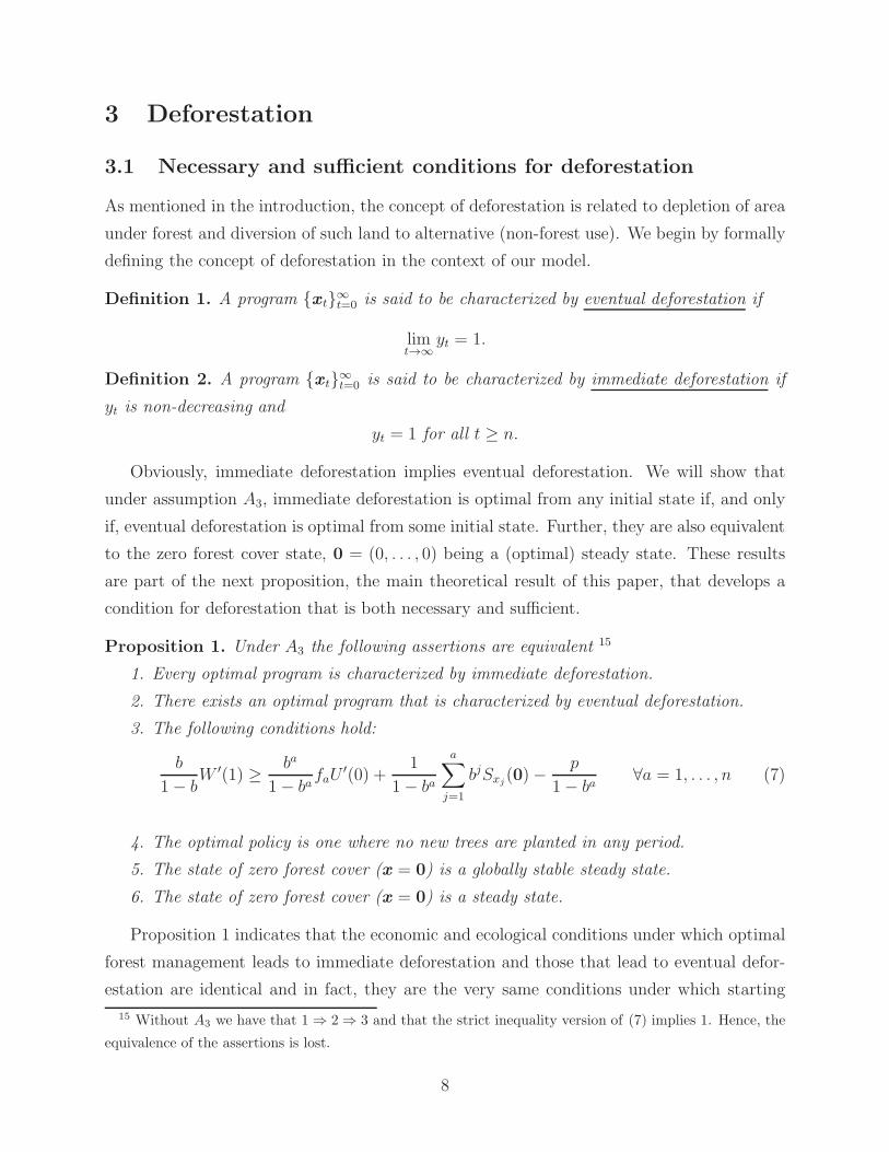
3.1 Necessary and sufficient conditions for deforestation

As mentioned in the introduction, the concept of deforestation is related to depletion of area

under forest and diversion of such land to alternative (non-forest use). We begin by formally

defining the concept of deforestation in the context of our model.

Definition 1. A program {x t}∞t=0 is said to be characterized by eventual deforestation if

limt→∞

yt = 1.

Definition 2. A program {x t}∞t=0 is said to be characterized by immediate deforestation if

yt is non-decreasing and

yt = 1 for all t ≥ n.

Obviously, immediate deforestation implies eventual deforestation. We will show that

under assumption A3, immediate deforestation is optimal from any initial state if, and only

if, eventual deforestation is optimal from some initial state. Further, they are also equivalent

to the zero forest cover state, 0 = (0, . . . , 0) being a (optimal) steady state. These results

are part of the next proposition, the main theoretical result of this paper, that develops a

condition for deforestation that is both necessary and sufficient.

Proposition 1. Under A3 the following assertions are equivalent 15

1. Every optimal program is characterized by immediate deforestation.

2. There exists an optimal program that is characterized by eventual deforestation.

3. The following conditions hold:

b

1− bW ′(1) ≥

ba

1− bafaU

′(0) +1

1− ba

a∑

j=1

bjSxj(0)−

p

1− ba∀a = 1, . . . , n (7)

4. The optimal policy is one where no new trees are planted in any period.

5. The state of zero forest cover (x = 0) is a globally stable steady state.

6. The state of zero forest cover (x = 0) is a steady state.

Proposition 1 indicates that the economic and ecological conditions under which optimal

forest management leads to immediate deforestation and those that lead to eventual defor-

estation are identical and in fact, they are the very same conditions under which starting

15 Without A3 we have that 1 ⇒ 2 ⇒ 3 and that the strict inequality version of (7) implies 1. Hence, the

equivalence of the assertions is lost.

8

from a state where there is zero forest cover on land, it is optimal to not plant any new trees

and to remain in that state of zero forest cover forever. Under these conditions, the state of

zero forest cover becomes a globally stable steady state. Condition (7) provides a very tight

characterization of when all of these are optimal; it is a condition on the exogenous elements

of the model and is verifiable from its economic and ecological primitives.

The left hand side of (7) reflects the marginal (opportunity) cost of bringing some land

under forests once and forever; i.e., the foregone benefit from alternative use. The right

hand side of (7) captures the marginal benefit from planting trees; this includes the marginal

benefit from timber harvesting (realized at the points of time the planted trees are harvested)

and the flow of marginal stock benefits from the standing trees until their harvest minus the

cost of planting trees. Condition (7) requires that starting from a state of zero forest cover,

the dynamic marginal cost of planting trees exceeds the dynamic marginal benefit of doing

so. This suggests that it is not optimal to move from a state of zero forest cover i.e., that the

latter is an optimal steady state. The fact that this condition also implies that it is optimal

to converge to this steady state in finite time from any state (i.e., independent of the extent

of forest cover and the age structure of the forest) is the interesting part of Proposition 1.

It is easy to see from condition (7) that low timber content of trees, low price for timber

(low marginal benefit from timber harvesting), high planting cost and high marginal return

on alternative use are likely to create greater incentives for deforestation. On the other hand,

technological changes that increase the timber content (or forest growth) or reduce harvesting

costs are likely to encourage conservation of forests. An increase in the stock benefits from

standing forests internalized by the forest manager also encourages conservation.

Observe that as b > 0, if U ′(0) = ∞, then deforestation can never occur (no matter how

much the future is discounted). It is already known that in this case, timber consumption

must be positive in every time period, but the contribution of Proposition 1 is stronger: if

U ′(0) = ∞, there is no optimal program along which the forest cover converges to zero.

However, the area of forest cover might be very small.

Though we assume b > 0, it is easy to check that in our framework deforestation is always

optimal for a myopic decision maker with b = 0. Further, if U ′(0) < ∞ then (7) is always

satisfied and deforestation is optimal if b > 0 is small enough. However, the effect of an

increase in the discount factor b is ambiguous as both sides of (7) are increasing in b. More

assumptions are necessary to determine the effect of the variations of b. We will elaborate

more in this effect in the next subsection, when the function S(x) depends only on the total

timber content of the standing forest.

9

3.2 Implications for Public Policy

Much of the stock benefits from standing forests (such as carbon sequestration) are in the

nature of environmental externalities that are typically not part of the cost-benefit calcula-

tions of a profit maximizing private owner (unless there is a regulatory structure to ensure

that these externalities are internalized). In this subsection, we use the general characteri-

zation in Proposition 1 to focus on the difference between the private and social incentives

to engage in deforestation. In particular, we compare the condition for deforestation when

the forest is managed by a private owner that ignores all stock benefits to that of a social

planner who takes into account these stock benefits. When deforestation is privately but not

socially optimal, we examine how simple public subsidy schemes can be designed to provide

incentives to a private owner to avoid deforestation.

For simplicity, we assume that the direct social benefit from timber harvest is identical

to the private owner’s benefit or profit; this holds for instance, if the timber harvest is

entirely exported. As a result, the only difference between the private and social optimization

problems is that the former sets stock benefits equal to zero.

In the absence of any public policy or regulation, a private owner solves Problem (4)

taking S(x) ≡ 0. The necessary and sufficient condition for deforestation (7) then reduces

tob

1− bW ′(1) ≥

ba

1− bafaU

′(0)−p

1− ba∀a = 1, . . . , n (8)

The social planner however does takes into account the stock externalities from the

standing forest. For simplicity, we impose some more structure on the nature of stock

benefits or externalities by assuming that it depends only on the total timber content of the

standing forest i.e.,

S(x t) = A

(n∑

a=1

faxa,t

).16 (9)

In addition, we impose the following assumption on A(·),

A′2: A is concave, non-decreasing, continuous in IR+ and differentiable in IR++.

It is easy to see that if A(·) satisfies A′2 then S(x) = A(

∑n

a=1 faxa,t) satisfies A2. Once

16A very similar option is to take subsidies that are a function of the total forestry area, f(∑

axa,t

),

which can also be viewed as a tax on the alternative use, as∑

axa,t = (1 − yt). As the analysis for these

two options are analogous we will only present our results when the subsidy depends on the total standing

biomass leaving the details of the latter case to the reader.

10

again, using (7) we have that deforestation is socially optimal if and only if

b

1− bW ′(1) ≥

ba

1− bafaU

′(0) +1

1− baA′(0)

a∑

j=1

bjfj −p

1− ba∀a = 1, . . . , n (10)

It is easy to check that the right hand side of (8) is smaller than or equal to that of (10) i.e.,

deforestation is privately optimal if it is socially optimal, but for a subset of the parameter

space deforestation is privately optimal but not socially optimal.

While it is always possible to fully align the private owner’s incentives with the social

planners by using a nonlinear subsidy, we want to focus on a simple subsidy scheme. We will

consider subsidies that are linear in total timber content of the standing forest. In particular,

in each period t, the total subsidy received by the private owner is λ∑

a faxa,t where λ ≥ 0.

With such a subsidy, the private owner now solves the optimization problem (4) where

S(x) = λ∑

a

faxa,t. (11)

Note that the specific form (11) of stock benefits is a special case of (9) and satisfies assump-

tion A2. Using (7), a private owner receiving such a subsidy will engage in deforestation if

and only if

b

1− bW ′(1) ≥

ba

1− bafaU

′(0) +λ

1− ba

a∑

j=1

bjfj −p

1− ba∀a = 1, . . . , n

Deforestation is avoided if λ satisfies:

λ > mina

{ 1∑a

j=1 bjfj

[p+ b

1 − ba

1− bW ′(1)− bafaU

′(0)]}

. (12)

This gives us an explicit lower bound on the subsidy needed to avoid deforestation and

indicates that forest stock subsidies that are lower than a critical level are unlikely to have

any effect on deforestation (small interventions are ineffective).

If (8) holds but (10) does not hold, i.e., deforestation is privately but not socially optimal,

A′(0) is greater than the right hand side of (12). While a subsidy equal to A′(0), the marginal

stock benefit at zero, can definitely avoid deforestation, we can achieve the same by a smaller

subsidy that lies between the right hand side of (12) and A′(0).

Note that improvement in timber content, the timber planting technology and increase

in the price at which timber can be sold (increase in demand for timber) reduce the minimal

subsidy needed to avoid deforestation. As long as deforestation is not socially optimal,

any further increase in stock benefit from forests does not affect the subsidy needed to avoid

11

deforestation. On the other hand, the minimal subsidy is increasing in p, the cost of planting

trees, and in W ′(1), the marginal benefit from alternative use of land (at zero forest cover);

both discourage forestry. Finally, if we assume that the biomass coefficients are increasing

in age, then it can be shown that minimal subsidy decreases with an increase in the discount

factor i.e., milder discounting promotes forest conservation. We prove this in Remark 1 in

the Appendix.

Of course, even if deforestation is avoided, the forest cover ensured by this subsidy can

be arbitrarily small. The next section discusses how a subsidy can be designed to ensure

that the forest cover is at a socially optimal level.

4 Minimum forest cover

When economic and ecological conditions rule out deforestation, it is of interest to understand

the amount forest cover that is sustained over time. Now, if the (necessary and sufficient)

condition for deforestation (7) in Proposition 1 does not hold, then all we know is that

limt→∞

inf yt < 1,

so that not only can the amount of forest cover be arbitrarily small but in fact, the forest

cover may actually be zero along a subsequence of time periods. In this paper, we do not

focus on characterizing these possibilities (though an optimal path that cycles between zero

and positive forest cover would be qualitatively consistent with existing results on periodic

cycles in models of forest management). Instead, we will characterize the minimum forest

cover that must be sustained along the optimal path.

In what follows, we assume that (7) does not hold for at least one value of a so that

deforestation is not optimal. Further, we impose an additional assumptions on the function

S. Let m the index of the maximal biomass coefficient (i.e., fm ≥ fa for all a = 1, . . . , n).

Let em be the unit vector such that em = 1 and ea = 0 for all a 6= m. We assume

A4: Sa(x) ≥ Sa(em

∑j xj) for all a = 1, . . . , n and for all x ∈ D.

Although A4 seems difficult to verify in general, it is satisfied if S depends only the total

standing biomass (as in (9)) or the total area under forest, and it is a concave function.

We assume A1, A2 and A4 for all the results in this section.

12

4.1 Deriving the minimum forest cover

We start defining the auxiliary functions ga(y), a = 1, . . . , n, where

ga(y) = p+ b1− ba

1− bW ′(y)− bafaU

′(fm(1− y))−a∑

j=1

bjSj((1− y)em). (13)

Using A1 and A2, one can check that ga is continuous and decreasing for all a = 1, . . . , n.17

Let ya be defined by:

ya = sup {y ∈ [0, 1] : ga(y) ≥ 0} (14)

where ya = 0 if ga(0) < 0. Besides, if ga(0) ≥ 0 and ga(1) ≤ 0 then ya is the largest (unique,

if ga is strictly decreasing) solution to ga(y) = 0 in [0, 1].

The next result identifies upper bounds on the area under alternative use.

Lemma 2. Let {x t}∞t=0 be an optimal program. Then,

minj=1,...,a

{yt+j} ≤ ya ∀a, ∀t ≥ 0.

The next proposition, which follows immediately from the above lemma, outlines lower

bounds on the forest cover.

Proposition 2. Let {x t}∞t=0 be an optimal program and let ya be as defined in (14). Then

the following holds:

maxj=1,...,a

{1− yt+j} ≥ 1− ya ∀a, ∀t > 0,

i.e., the forest cover is above 1− ya at least once every a periods.

We single out the case a = 1 for its importance in terms of the conclusions that can be

obtained. The proposition above implies that, in particular,

Corollary 1. 1− yt ≥ 1 − y1 ∀t > 0, i.e., the forest cover is at least as large as 1 − y1 at

every time period.

Observe that ga(1) ≥ 0 ∀a if, and only if, (7) holds. Hence, in the absence of deforestation,

we have ga(1) < 0 for at least one value of a. Whenever g1(1) < 0, we have y1 < 1, i.e.,

the forest cover is bounded away from zero which can be thought of as strong avoidance of

deforestation. Whenever ga(1) < 0 for some value of a > 1, we have ya < 1, i.e., there is

partial forest cover at least once every a periods - a somewhere weaker form of avoidance of

deforestation. If U ′(0) = ∞, 1− ya > 0 for all a.

17They are strictly decreasing if either U or W is strictly concave or S1 is strictly decreasing with respect

to xm.

13

Corollary 2. The following hold

• If g1(0) < 0, i.e., if

p+ bW ′(0)− bf1U′(fm)− bS1(em) < 0 (15)

then y1 = 0 and there is full forest cover every period.

• If ga(0) < 0, i.e., if

p+ b1− ba

1− bW ′(y)− bafaU

′(fm)−

a∑

j=1

bjSj(em) < 0 (16)

then ya = 0 and there is full forest cover at least once every a periods.

Note that high planting cost or high marginal benefit from alternative use increase the

value of yaA for a = 1, . . . , n, implying that we have a smaller lower bound on forest cover.

Further, a decrease in the discount factor b, is likely to increase the value of yaA implying

that the lower bound on forest cover is reduced. On the other hand, an increase on the price

of timber or in the marginal benefit from standing forest stock is likely to decrease the value

of yaA implying that we have a larger lower bound on forest cover. Finally, the effect of a

technological change that increases timber content or reduces harvesting cost is ambiguous;

we need more specific structure to obtain definite predictions.

4.2 Implications for Public Policy

To see how Proposition 2 can provide specific guidelines for public policy, we revert to the

specific framework in subsection 3.2 where we consider a private owner that ignores all stock

benefits (set S(·) = 0), a social planner that takes into account all stock benefits (where S(·)

depends only on the total timber content as specified in (9)) and finally, a public subsidy

policy where the subsidy is linear in the total timber content (i.e., of the form λ∑

a faxa).18

Note that the specific form of the stock benefit function S(x) = A(∑

a faxa) used by the

social planner satisfies A2 and A4 whenever A fulfills A′2. Further, with the linear subsidy,

the private owner sets S(x) = λ∑

a faxa and this satisfies A4. The auxiliary functions in

(13) can now be re-written for each of the above mentioned cases. In the social planner’s

problem, the corresponding ga function is

gaA(y) = p+ b1− ba

1− bW ′(y)− bafaU

′(fm(1− y))− A′(fm(1− y))

a∑

j=1

bjfj

18This is just a specific version of Pigou tax for externalities [21].

14

and in the subsidized private owner facing linear subsidy λ∑

a faxa it is given by

gaλ(y) = p+ b1− ba

1− bW ′(y)− bafaU

′(fm(1− y))− λ

a∑

j=1

bjfj

The definitions of yaA and yaλ are analogous to (14).

To ensure that in the problem faced by the subsidized private owner the lower bound

on the forest cover y1λ coincides with the socially optimal lower bound y1A it is sufficient to

choose subsidy rate λ equal to

λ1 = A′(fm(1− y1A)) (17)

If, on the other hand, to ensure that the “at least once every a periods”-lower bound on the

forest cover yaA is also met by the private owner, the subsidy rate λ can be set equal to

λa = A′(fm(1− yaA)). (18)

Under assumption A′2, these values of λ are non-negative.

5 Example

To illustrate the conditions presented in the previous sections, we provide a numerical ex-

ample. We consider a dual aged forest (n = 2) where the biomass coefficients are f1 = 0.45

and f2 = 1. 19 We choose a discount factor b = 0.9. We assume that the benefit functions

U and S are quadratic and W is linear; in particular,

U(c) = α1c−α2

2c2 with α1 = 2, α2 = 0.8

A(x) = β1x−β2

2x2 with β1 = 1.5, β2 = 0.4

W (y) = ωy with ω = 1.25

With these parameters’ values, it is easy to check that while (10) is not satisfied, (8)

holds. We are then in a situation where deforestation is privately but not socially optimal in

the absence of subsidies. If we design a simple subsidy that is linear in total timber content

i.e., of the form λ∑

a faxa, then (12) implies that to avoid total deforestation the parameter

λ must be larger than

min

{1

bf1(p+ bω)− α1,

1

bf1 + b2f2[p+ (b+ b2)ω − bα1]

}≈ 0.59

19[22, 27] contain an analysis of the Mitra-Wan model for the special case of a dual aged forest (n = 2)

which allows for sharper theoretical results.

15

Now suppose the objective of public policy is to go beyond the simple avoidance of total

deforestation and try to ensure certain lower bounds on the forest cover (in the privately

optimal path). With the parameters’ values defined above we find that y1A ≈ 0.81 and

y2A ≈ 0.03. From (17), we see that if the social planner wants to assure a minimal forest

cover (derived from the social planner’s problem) of 1 − y1A ≈ 0.19 every time period, the

subsidy rate λ1 must be at least A′(f2(1 − y1A)) ≈ 1.42. If, on the other hand, if the social

planner is satisfied with assuring 1 − y2A ≈ 0.97 at least once every two periods, then the

subsidy can be smaller, from (18) we see that it is sufficient to choose the subsidy rate

λ2 ≥ A′(f2(1− y2A)) ≈ 1.11.

It is somehow surprising that λ2 is smaller than λ1, as the value of the second lower

bound imposed is much larger than the first one. The smaller value of λ2 is due to the fact

the forest cover must be above (1− y2A) only once every two periods. This suggests that the

forest cover may present large oscillations along the optimal trajectory.

It is also interesting to note that if we take λ1 = 1.42, to assure that the lower bound on

forest cover (from the social planner’s problem) is satisfied in every time period, the value

for y2λ is zero, meaning that there is total forest cover at least once every two periods. On the

other hand, if we take λ2 = 1.11 to assure that the minimal bound once every two periods is

satisfied, then the value of y1λ is one, implying that there could be zero forest cover in some

periods (at most once every two time periods).

Finally, if the social planner wants to assure full forest cover in every period, she must

offer a subsidy that ensures that y1λ = 1, i.e., p + bW ′(0) − bf1 [U′(f2) + λ] < 0 (see (15)),

implying that λ must be larger than or equal 1bf1

(p+ bW ′(0)

)− bU ′(f2) ≈ 2, 07.

6 Extensions

Our paper has not addressed the problem of characterization of steady states and their

stability in situations where total deforestation is not optimal; this remains an open question

in the context of our general model. Our current analysis indicates that in a simplified version

of the model, where n = 2, a characterization of the transition dynamics and comparative

dynamics of important parameters, as in [8], may be possible.

More research is needed to examine how our conditions for deforestation are modified if

the model is extended to allow for other realistic features such as irreversibility of deforesta-

tion, soil erosion and uncertainty.

In particular, irreversibility arises when land under alternative use is rendered unsuitable

16

for future reforestation. Whether or not such an irreversibility is relevant depends on the

nature of alternative use as well as the composition of the forest. It is easy to see that

introduction of such irreversibility in our model reduces the set of feasible programs; every

program that meets the irreversibility constraint is also feasible in our model but the reverse

is not true as programs involving diversion of land from alternative use to forests are no

longer admissible. This implies that if some program is optimal in our model (where there is

no irreversibility) and in addition, satisfies the irreversibility constraint, then it must be op-

timal in the model with irreversibility. In particular, a program characterized by immediate

deforestation in our model involves no reversal of land use from alternative use to forestry

and therefore continues to be feasible with irreversibility. Therefore, the conditions under

which deforestation is optimal in our model are also sufficient to ensure that deforestation

is optimal under irreversibility. However, with irreversibility, deforestation may be optimal

under weaker conditions. For instance, if the initial state is one where all land is dedicated

to alternative use then the only feasible program under full irreversibility involves deforesta-

tion. But (as we have shown) without irreversibility, if our conditions for deforestation do

not hold then from the same initial state it is optimal to sustain positive forest cover in-

finitely often. Thus, introducing irreversibility in diversion of land to alternative use makes

deforestation more likely.20 However, this may be modified if there is uncertainty about

future benefits of forest use and irreversibility may create an option value for conservation

of forests. Indeed, several previous studies [4, 11] have shown that in the presence of irre-

versibility, uncertainty about the future can make depletion of irreplaceable assets less likely.

The study of deforestation under irreversibility and uncertainty remains an important topic

for future research.

Our analysis in this paper is carried out under the assumption that the total area of

available land for forest and non-forest use is fixed; this allows us to focus on the dynamic

tradeoff between forest and non-forest use where the dynamic value of having forest cover is

endogenously determined through control of age distribution. However, in many real world

situations, diversion of land to alternative use reduces the total amount of land through

soil erosion. Intuitively, this should increase the incentive for forest conservation and make

deforestation less likely. Mathematically, introducing such a law of motion for the total area

20Instead of full irreversibility, we can think of a situation where reforestation is possible at some cost.

Then, a term representing the cost of conversion of land from alternative use to forests must be included

in the objective function. With partial irreversibility the perturbation analysis performed in the proof of

Lemma 1 can be done, with new terms appearing in equations (5) and (6) whenever land is converted to

forestry. This asymmetry breaks the equivalence obtained in Proposition 1.

17

of available land makes the optimization problem intrinsically more complicated than the

one studied in this paper, but the insights it may provide makes it worth studying in the

future.

7 Conclusion

Deforestation is a complex social phenomenon. In this paper, we have tried to understand

the broad economic and ecological conditions under which deforestation may occur even

though there is no failure of property rights and the forest is managed effectively. Our

analysis has been carried out in the context of a very well known economic model of optimal

forest management (the Mitra-Wan model) that we have extended to allow for benefits from

standing forests (in addition to timber harvests) and alternative use of land. Despite the

fact that optimal paths in this class of models may be characterized by cycles and steady

states that are not globally stable, we obtain a very sharp characterization of deforestation.

We show that if deforestation occurs from any initial state then it must occur in finite time

from every initial state. As a result, a “local” condition that simply rules out any incentive

to move away from a state of zero forest cover turns out to be necessary and sufficient for

global deforestation. The comparative statics of this condition clearly shows that factors that

improve profitability of (or more generally the marginal benefit from) harvesting timber such

as an increase in price of timber (increase in demand) or reduction in the cost of harvesting

tend to promote conservation of forests. Similarly, an increase in the flow benefits from

standing forests that are internalized by forest management (for instance, as a consequence

of public policy) make deforestation less likely. We also derive a precise bound on forest

cover that is relevant to situations where deforestation is not optimal. We demonstrate how

our general results can be used to study the wedge between private and social optimality

of deforestation, and suggest a simple subsidy on standing forests that can induce a private

owner to conserve forests or maintain a minimal level of forest cover.

To the best of our knowledge, this is the first paper to attempt to derive analytical

conditions for deforestation and in doing so, it contributes to the general economic theory

of extinction and conservation of natural resources.

Acknowledgments

Adriana Piazza is grateful of the hospitality of the Southern Methodist University where

18

this research was initiated and acknowledges the financial support of Fondecyt 1140720,

Programa Basal 03, CMM, U. de Chile and Project Anillo ACT-1106.

A Proofs

Proof of Lemma 1. We define the unitary vector e j ∈ IRn such that ej = 1 and ek = 0 for

all k 6= j. Consider an alternative program {xs}∞s=0 such that

x t+j = x t+j + ǫe j ∀j = 1, . . . , a.

xs = xs else

In words, whenever ǫ > 0 (ǫ > 0), the alternative program is one where the area under

alternative use is reduced (increased) by ǫ at time period t + 1 and replanted to yield

more (less) young forest next period. This modification of the young forest area is let to

propagate until age a at which point the consumption of forest of age a is modified. Of

course, the area under alternative use, can only be reduced if it is strictly positive along the

periods involved, i.e., minj=1,...,a{yt+j} > 0. On the other hand, to increase the land under

alternative use along the time periods t + 1, . . . , t + a, we decrease the harvest of age class

a at time t + a, hence we need ca,t+a > 0. In conclusion, the alternative program is feasible

for −ca,t+a < ǫ < min{yt+1, yt+2, . . . , yt+a}.

As {x t}∞t=0 is optimal, the modification must give a smaller benefit, hence:

∞∑

t=1

bt−1[U(ct) +W (yt) + S(x t)− px1,t+1] ≥

∞∑

t=1

bt−1[U(ct) +W (yt) + S(x t)− px1,t+1]

which is equivalent to

baU(ct+a) +a∑

j=1

bj [W (yt+j) + S(x t)]− px1,t+1 ≥

baU(ct+a + faǫ) +

a∑

j=1

bj [W (yt+j − ǫ) + S(x t + ǫea)]− p(x1,t+1 + ǫ),

and reordering we get

pǫ+a∑

j=1

bj [W (yt+j)−W (yt+j − ǫ)] ≥ (19)

ba[U(ct+a + faǫ)− U(ct+a)] +

a∑

j=1

bj [S(x t + ǫea)− S(x t)]

19

If minj=1...a{yt+j} > 0 we can consider ǫ > 0. Dividing through by ǫ and taking the limit as

ǫ → 0+, we obtain inequality (5).

If ca,t+a > 0 we can consider ǫ < 0. Dividing through by ǫ < 0 and taking the limit as

ǫ → 0−, we obtain inequality (6).

Proof of Proposition 1. We see first that 1, 2, 3 and 4 are equivalent by showing that 1 ⇒

2 ⇒ 3 ⇒ 4 ⇒ 1.

From the definitions of total deforestation and eventual deforestation it is evident that 1

⇒ 2.

Let us show that 2 ⇒ 3. Let {x t}∞t=0 be an optimal program characterized by eventual

deforestation. As {yt} → 1, there exists T such that yt > 0 for all t ≥ T. Using Lemma 1,

we have that (5) holds for all a and t ≥ T. Observe that as {yt} → 1,{xa,t} → 0 for all a

so that taking the limit as t → ∞ on both sides of the inequalities (5) and rearranging the

terms we obtain (7).

We turn now to the proof that 3 ⇒ 4. We want to show that under (7), it is optimal to

never re-plant, i.e., for any x0 ∈ D, the optimal policy is such that x1,t = 0 for all t > 0. To

show the optimality of such a policy, suppose to the contrary that there exists x0 ∈ D such

that there is an optimal program from this initial state where

x1,1 > 0.

The trees that are one year old at t = 1 must be harvested at some time period. Hence there

is at least one value of a = 1, . . . , n such that ca,a > 0. From Lemma 1, we have that (6)

holds for t = 0 i.e.,

p+

a∑

j=1

bjW ′(yj) ≤ bafaU′(ca) +

a∑

j=1

bjSj(xj)

and using the strict concavity of U on a neighborhood of zero, A1 and A2 we have:

p+

a∑

j=1

bjW ′(1) < bafaU′(0) +

a∑

j=1

bjSj(0)

which violates (7).

Finally, to see that 4 ⇒ 1, simply observe that if x1,t = 0 for all t > 0 all forest is

transferred to alternative use, after at most n periods, and stays that way forever.

This completes the first part of the proof. The equivalence of the last two assertions

follows almost directly. Indeed, it is evident that 5 ⇒ 6. It is also easy to see that 1 ⇒ 5.

20

Finally, if 6 holds then the program x t = 0 and yt = 1 ∀t is optimal and characterized by

eventual deforestation, yielding that 6 ⇒ 2.

Remark 1. While it is very easy to see that the terms p∑j b

jfjand −bafaU

′(0) in (12) are

decreasing with b, proving that 1−ba

(1−b)∑

j bjfj

bW ′(1) is decreasing entails a more much com-

plicated calculation and depends on f1 ≤ f2 ≤ · · · ≤ fn. Indeed, it can be proved that the

derivative of this last term is

W ′(1)1

(∑n−1

j=1 bj−1fj)2

n−1∑

a=1

[(fa − fa+1)︸ ︷︷ ︸

≤0

n−1∑

i=a

(ibi−1 +

a−1∑

j=1

(i− j)bi+j−1)

︸ ︷︷ ︸≥0

]≤ 0.

Proof of Lemma 2. Let us denote by y = minj=1,...,a{yt+j}. If y = 0 the inequality holds

trivially. If y > 0, we know thanks to (5) that

0 ≤ p+a∑

j=1

bjW ′(yt+j)− bafaU′(ct+a)−

a∑

j=1

baSj(x t+j)

≤ p+

a∑

j=1

bjW ′(yt+j)− bafaU′(fm

n∑

a=1

xa,t+j)−

a∑

j=1

baSj(em

n∑

a=1

xa,t+j)

= p+a∑

j=1

bjW ′(yt+j)− bafaU′(fm(1− yt+j))−

a∑

j=1

baSj(em(1− yt+j)

≤ p+

a∑

j=1

bjW ′(y)− bafaU′(fm(1− y))−

a∑

j=1

baSj(em(1− y)) = ga(y).

This implies that ga(minj=1,...,a{yt+j}) ≥ 0, and hence, minj=1,...,a{yt+j} ≤ ya.

References

[1] Gregory S. Amacher, Marku Ollikainen, Erkki A. Koskela, Economics of Forest Re-

sources, MIT Press, 2009.

21

[2] Arild Angelsen, David Kaimowitz, Rethinking the Causes of Deforestation: Lessons from

Economic Models, The World Bank Research Observer 14 (1999) 73–98.

[3] Peter Berck, The Economics of Timber: A Renewable Resource in the Long Run, The

Bell Journal of Economics,10(2),1979, 447-462/

[4] Kenneth J. Arrow, Anthony C. Fisher, Environmental Preservation, Uncertainty, and

Irreversibility, The Quarterly Journal of Economics, 88(2), 1974, 312-319.

[5] Michael D. Bowes, John V. Krutilla, Multiple use management of public forestlands, In

Handbook of natural resource and energy economics 2, 1985, 531–569.

[6] Michael D. Bowes, John V. Krutilla, Multiple use management: the economics of public

forestlands, Resources for the Future Press, Washington, D.C., 1989

[7] Colin W. Clark, Profit Maximization and the Extinction of Animal Species, Journal of

Political Economy, 81(4), 1973, 950-961.

[8] Swapan Dasgupta, Tapan Mitra, On optimal forest management: A bifurcation analysis,

In Dimensions of Economic Theory, Essays for Anjan Mukherjee, K.G. Dastidar, H.

Mukhopadhayay and U.B. Sinha (Eds.), Oxford University Press, 2011, 50-67.

[9] Global Forest Resources Assessment, FAO Forestry Paper 163, Food and Agriculture

Organization of the United Nations, 2010.

[10] Martin Faustmann, Berechnung des Wertes welchen Waldboden sowie noch nicht

haubare Holzbestande fur die Waldwirtschaft besitzen. Allgemeine Forst-und Jagd-

Zeitung 15, 1849, 7-44. Translated by W. Linnard, Calculation of the value which forest

land and immature stands possess for forestry, Journal of Forestry Economics 1, 1995,

7-44

[11] Claude Henry, Option Values in the Economics of Irreplaceable Assets, The Review of

Economic Studies, 41 (1974) 89-104.

[12] K. Norman Johnson, H. Lynn Scheurman, Techniques for prescribing optimal timber

harvest and investment under different objectives–discussion and synthesis, Forest Sci-

ence, 23(Supplement 18), 1977, a0001-z0001.

[13] M. Ali Khan, Adriana Piazza, On the Mitra-Wan forestry model: a unified analysis,

Journal of Economic Theory, 147(1) (2012) 230-260.

22

[14] Kenneth S. Lyon, Mining of the forest and the time path of the price of timber, Journal

of Environmental Economics and Management, 8(4), 1981, 330–344.

[15] Kenneth S. Lyon, Roger A. Sedjo, An optimal control theory model to estimate the

regional long-term supply of timber. Forest Science, 29(4), 1983, 798-812.

[16] Kenneth S. Lyon, Roger A. Sedjo, Binary-search SPOC: an optimal control theory

version of ECHO, Forest Science, 32(3), 1986, 576-584.

[17] Tapan Mitra, Henry Y. Wan Jr., Some Theoretical Results on the Economics of Forestry,

Review of Economics Studies LII (1985) 263–282.

[18] Tapan Mitra, Henry Y. Wan Jr., On the Faustmann solution to the forest management

problem, Journal of Economic Theory 40 (1986) 229-249.

[19] David W. Pearce, The Economic Value of Forest Ecosystems, Ecosystem Health 7 (2001)

284–296.

[20] Lars J. Olson, Santanu Roy, On Conservation of Renewable Resources with Stock-

Dependent Return and Non-Concave Production, Journal of Economic Theory 70 (1996)

133–157.

[21] Arthur C. Pigou, The Economics of Welfare, London: Macmillan, 1932.

[22] Seppo Salo, Olli Tahvonen, On equilibrium cycles and normal forests in optimal harvest-

ing of tree vintages, Journal of Environmental Economics and Management 44 (2002)

1–22.

[23] Seppo Salo, Olli Tahvonen, On the economics of forest vintages, Journal of Economic

Dynamics and Control 27 (2003) 1411–1435.

[24] Seppo Salo, Olli Tahvonen, Renewable resources with endogenous age classes and allo-

cation of land, American Journal of Agricultural Economics 86 (2004) 513–530.

[25] Olli Tahvonen, Optimal harvesting of forest age classes: a survey of some recent results,

Mathematical Population Studies 11(3-4) (2004) 205–232.

[26] Olli Tahvonen, Timber production versus old-growth preservation with endogenous

prices and forest age-classes, Canadian Journal of Forestry Research 34, 2004, 1296-

1310.

23

[27] Henry Y. Wan Jr., Revisiting the Mitra-Wan tree farm, International Economic Review

35 (1994) 193–198.

24