PI2: A Linearized AQMfor both Classic and Scalable TCP

Koen De Schepper† Olga Bondarenko∗‡ Ing-Jyh Tsang† Bob Briscoe‡

†Nokia Bell Labs, Belgium ‡Simula Research Laboratory, Norway†{koen.de_schepper|ing-jyh.tsang}@nokia.com ‡{olgabo|bob}@simula.no

ABSTRACTThis paper concerns the use of Active Queue Manage-ment (AQM) to reduce queuing delay. It offers insightinto why it has proved hard for a Proportional Inte-gral (PI) controller to remain both responsive and sta-ble while controlling ‘Classic’ TCP flows, such as TCPReno and Cubic. Due to their non-linearity, the con-troller’s adjustments have to be smaller when the targetdrop probability is lower. The PI Enhanced (PIE) al-gorithm attempts to solve this problem by scaling downthe adjustments of the controller using a look-up table.Instead, we control an internal variable that is by defini-tion linearly proportional to the load, then post-processit into the required Classic drop probability—in fact weshow that the output simply needs to be squared. Thisallows tighter control, giving responsiveness and stabil-ity better or no worse than PIE achieves, but withoutall its corrective heuristics.

With suitable packet classification, it becomes simpleto extend this PI2 AQM to support coexistence betweenClassic and Scalable congestion controls in the publicInternet. A Scalable congestion control ensures suffi-cient feedback at any flow rate, an example being DataCentre TCP (DCTCP). A Scalable control is linear, sowe can use the internal variable directly without anysquaring, by omitting the post-processing stage.

We implemented PI2 as a Linux qdisc to extensivelytest our claims using Classic and Scalable TCPs.

1. INTRODUCTIONInteractive latency-sensitive applications are becom-

ing prevalent on the public Internet, e.g. Web, voice,

∗The first two authors contributed equally

Permission to make digital or hard copies of all or part of this work for personalor classroom use is granted without fee provided that copies are not made ordistributed for profit or commercial advantage and that copies bear this noticeand the full citation on the first page. Copyrights for components of this workowned by others than the author(s) must be honored. Abstracting with credit ispermitted. To copy otherwise, or republish, to post on servers or to redistribute tolists, requires prior specific permission and/or a fee. Request permissions frompermissions@acm.org.

CoNEXT ’16, December 12 - 15, 2016, Irvine, CA, USAc© 2016 Copyright held by the owner/author(s). Publication rights licensed to

ACM. ISBN 978-1-4503-4292-6/16/12. . . $15.00

DOI: http://dx.doi.org/10.1145/2999572.2999578

conversational and interactive video, finance apps, on-line gaming, cloud-based apps, remote desktop. It hasbeen conjectured that there is also latent demand formore interactivity and new interactive apps would sur-face if there were less lag in the public Internet [10].In the developed world, increases in access network bit-rate have been giving diminishing returns as latencyhas become the critical bottleneck. Recently, much hasbeen done to reduce propagation delay, e.g. by placingcaches or servers closer to users. However, latency is amulti-faceted problem [7], so other sources of delay suchas queuing have become the bottleneck.

Queuing delay problems occur when a capacity-seeking (e.g. TCP) traffic flow is large enough to lastlong enough to build a queue in the same bottleneckas traffic from a delay-sensitive application. Thereforequeuing delay only appears as an intermittent prob-lem [17]. Nonetheless, perception of quality tends tobe dominated by worst case delays and many real-timeapps adapt their buffering to absorb all but worst-casedelays.

To remove unnecessary queuing delays, Active QueueManagement (AQM) is being deployed at bottlenecks.AQM introduces a low level of loss, to keep the queueshallow within the buffer. However, for an AQM toreduce queuing delay any further, it has to worsen dropand/or utilization. This is because the root cause ofthe problem is the behaviour of current TCP-friendlycongestion controls (Reno, Cubic, etc.). They behavelike a balloon; if the network squeezes one impairment,they make the others bulge out.

To remove one dimension from this trilemma, itwould seem Explicit Congestion Notification (ECN)could be used instead of loss. However, the meaningof an ECN mark was standardized as equivalent to aloss [30], so although standard (‘Classic’) ECN can re-move the impairment of loss itself, it cannot be used toreduce queuing delay relative to loss-based protocols.

Per-flow queuing has been used to isolate each flowfrom the impairments of others, but this adds a newdimension to the trilemma; the need for the networkto inspect within the IP layer to identify flows, not tomention the extra complexity of multiple queues.

Scalable

Classic

Classicsender

Scalablesender

Classifier drop or marker

Linear PI AQM

square

p'

Classicsender

drop or marker

Linear PI AQM

square

p'a)

b)

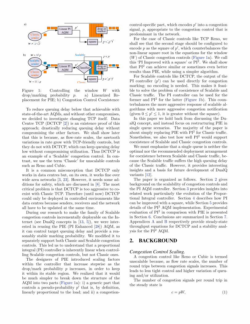
Figure 1: Controlling the window W withdrop/marking probability p. a) Linearized Re-placement for PIE; b) Congestion Control Coexistence

To reduce queuing delay below that achievable withstate-of-the-art AQMs, and without other compromises,we decided to investigate changing TCP itself. DataCentre TCP (DCTCP [2]) is an existence proof of thisapproach; drastically reducing queuing delay withoutcompromising the other factors. We shall show laterthat this is because, as flow-rate scales, the sawtoothvariations in rate grow with TCP-friendly controls, butthey do not with DCTCP, which can keep queuing delaylow without compromising utilization. Thus DCTCP isan example of a ‘Scalable’ congestion control. In con-trast, we use the term ‘Classic’ for unscalable controlssuch as Reno and Cubic.

It is a common misconception that DCTCP onlyworks in data centres but, on its own, it works fine overwide area networks [3, 23]. However, it needs some ad-ditions for safety, which are discussed in [8]. The mostcritical problem is that DCTCP is too aggressive to co-exist with Classic TCP. Therefore (until now) DCTCPcould only be deployed in controlled environments likedata centres because senders, receivers and the networkall have to be updated at the same time.

During our research to make the family of Scalablecongestion controls incrementally deployable on the In-ternet (see DualQ concepts in [13, 5]), we were inter-ested in reusing the PIE (PI Enhanced [28]) AQM, asit can control target queuing delay and provide a rea-sonably stable marking probability. We modified it toseparately support both Classic and Scalable congestioncontrols. This led us to understand that a proportionalintegral (PI) controller is inherently linear when control-ling Scalable congestion controls, but not Classic ones.

The designers of PIE introduced scaling factorswithin the controller that increase stepwise as thedrop/mark probability p increases, in order to keepit within its stable region. We realized that it wouldbe much simpler to break down the structure of theAQM into two parts (Figure 1a): i) a generic part thatcontrols a pseudo-probability p′ that is, by definition,linearly proportional to the load; and ii) a congestion-

control-specific part, which encodes p′ into a congestionsignal, p, appropriate to the congestion control that ispredominant in the network.

For the case of Classic controls like TCP Reno, weshall see that the second stage should be configured toencode p as the square of p′, which counterbalances thenon-linear square root in the equations for the window(W ) of Classic congestion controls (Figure 1a). We callthis ‘PI Improved with a square’ or PI2. We shall showthat PI2 can achieve similar or sometimes even betterresults than PIE, while using a simpler algorithm.

For Scalable controls like DCTCP, the output of thePI controller (p′) can be used directly for congestionmarking; no encoding is needed. This makes it feasi-ble to solve the problem of coexistence of Scalable andClassic traffic. The PI controller can be used for theformer and PI2 for the latter (Figure 1b). This coun-terbalances the more aggressive response of scalable al-gorithms with more aggressive congestion notification(given 0 ≤ p′ ≤ 1, it is greater without the square).

In this paper we hold back from discussing the Du-alQ concept, and instead focus on restructuring PIE insingle queue scenarios. The majority of the paper isabout simply replacing PIE with PI2 for Classic traffic.Nonetheless, we also test how well PI2 would supportcoexistence of Scalable and Classic congestion controls.

We must emphasize that a single queue is neither theoptimal nor the recommended deployment arrangementfor coexistence between Scalable and Classic traffic, be-cause the Scalable traffic suffers the high queuing delayof the Classic traffic. However, it provides interestinginsights and a basis for future development of DualQvariants [12].

The paper is organized as follows. Section 2 givesbackground on the scalability of congestion controls andthe PI AQM controller. Section 3 provides insights intorelated work particularly the evolution of the Propor-tional Integral controller. Section 4 describes how PIcan be improved with a square, while Section 5 providesdetails of the PI2 AQM implementation. Experimentalevaluation of PI2 in comparison with PIE is presentedin Section 6. Conclusions are summarized in Section 7.Appendices A and B respectively provide steady-statethroughput equations for DCTCP and a stability anal-ysis for the PI2 AQM.

2. BACKGROUND

Congestion Control Scaling.A congestion control like Reno or Cubic is termed

unscalable because, as flow rate scales, the number ofround trips between congestion signals increases. Thisleads to less tight control and higher variation of queu-ing and/or utilization.

The number of congestion signals per round trip inthe steady state is

c = pW, (1)

error

queue change

previous,τ(t-T)

current,τ(t)

target,τ

0

Δp = α(error) + β(queue change)

Figure 2: Basic PI algorithm

where W is the number of segments per round trip (thewindow) and p is the probability of congestion notifica-tion (either losses or ECN marks). Appendix A givesthe formulae for the steady-state window of various con-gestion controls, which are all of the form

W ∝ 1/pB , (2)

where B is a characteristic constant of the congestioncontrol.

The scalability of a congestion control can thereforebe determined by substituting for p from (2) into (1):

c ∝W (1−1/B). (3)

If B < 1, c shrinks as W scales up, which impliesfewer congestion signals per round trip (unscalable).Therefore, a congestion control is scalable if B ≥ 1 andunscalable otherwise.

From Appendix A, Reno and Cubic in its Reno mode(‘CReno’) have B = 1/2 and pure Cubic has B = 3/4,so all these ‘Classic’ controls are unscalable. WhileDCTCP with probabilistic marking has B = 1 and withstep marking it has B = 2. Therefore DCTCP is scal-able irrespective of the type of marking.

Proportional Integral (PI) AQM.The core of the PIE AQM is a classical Proportional

Integral (PI) controller [18] that aims to keep queuingdelay to a target τ0 by updating the drop probability,p, every update interval, T . Figure 2 recaps the basicPI algorithm, which consists of a proportional and anintegral part, weighted respectively by the gain factorsβ and α (both in units of Hz):

p(t) = p(t−T ) +α(τ(t)− τ0

)+β

(τ(t)− τ(t−T )

), (4)

where τ(t) is the queuing delay at time t. The propor-tional part estimates how much load exceeds capacityby measuring how fast the queue is growing. The inte-gral part corrects any standing queue due to the loadhaving exceeded capacity over time, by measuring theerror between the actual queuing delay and the target.Either term can be negative and the final probability isbounded between and including 0 and 1.

The proportional gain factor β can be seen as thebest known correction of p to reduce the excess load.The integral gain factor α is typically smaller than theproportional, and corrects any longer term offset fromthe target. Note that the integral part initially calcu-lates a proportional value, and the proportional part a

p

Drop/MarkDrop/Mark Feedback P[d] = p

p > Y

TCP Receiver

Classic TCP Sender

d

queue delayPI

Queue length

Scaling

α βTarget Delay

rate estimation

random()

Y

Figure 3: PIE AQM in Linux (additions to PI in green)

differential value. But these values are later integratedby adding them as a delta to the probability used in theprevious update interval.

3. RELATED WORKThe evolution of the Proportional Integral controller

Enhanced (PIE) AQM started with the control theo-retic analysis of RED by Holot et al [19], which ended bypointing out that it was not necessary to adopt the ap-proach of RED, which pushes back against higher loadwith higher queuing delay and higher loss. Instead, in[18], the same authors presented a Proportional Inte-gral (PI) controller, using classical linear systems anal-ysis with the objective of holding queuing delay to aconstant target, using higher loss alone to push backagainst higher load.

This PI controller was used as the basis of the IEEEData Centre Bridging (DCB) standard, 802.1Qau [15],published in 2010. Variants of the original PI AQM con-troller had also been proposed in the research commu-nity. In 2004, Hong et al claimed that the phase marginof the original PI controller could be over-conservative,leading to unnecessarily sluggish behaviour. Instead,they proposed a design [21] that would self-tune to thespecified phase margin. In 2007, Hong and Yang [20]proposed to self-tune the gain margin instead, and totrigger the self-tuning process whenever it moved out-side an operating range. However implementations havenot adopted these self-tuning designs, probably becausethey require code to estimate the average (harmonicmean) round trip time of the TCP flows, which in turndepends on estimating the number of TCP flows, thelink capacity and the equilibrium dropping probability,p. Of course, p is itself the output of the controller and,by definition, determining its equilibrium value is prob-lematic when network conditions are changing, which iswhen self-tuning is required.

In 2013, the Proportional Integral controller En-hanced (PIE [28]) was proposed as an evolution ofthe original PI algorithm [18]. After extensive evalu-ation [32], PIE became the mandatory AQM algorithmfor DOCSIS3.1 cable modems [9] and it is also beingdocumented in an IETF specification [29].

Figure 3 shows the building blocks of the Linux PIEAQM implementation. PIE introduced three enhance-ments over PI. The first was to use units of time (notbytes or packets) for the queue, to hold queuing de-lay constant whatever the link rate. This ensures the

p [%]

30

20

10

0

-10

-20

-301001010.10.010.0010.0001

Phas

e M

argi

n [d

eg]

90

45

0

-45

-90

Gai

n M

argi

n [d

B]

tune=1/8tune=1/2tune=1tune=auto

Figure 4: Bode plot margins for R=100 ms,αPIE=0.125*tune, βPIE=1.25*tune, T=32 ms

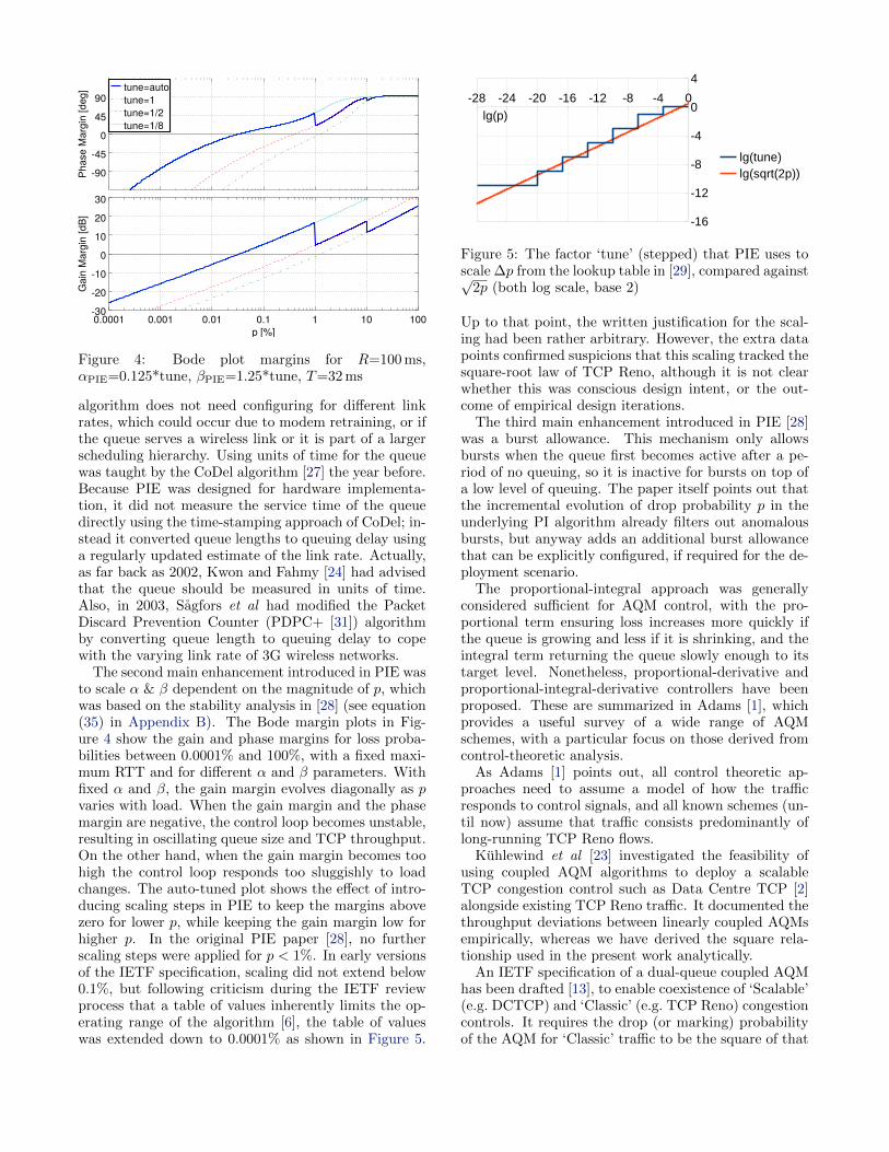
algorithm does not need configuring for different linkrates, which could occur due to modem retraining, or ifthe queue serves a wireless link or it is part of a largerscheduling hierarchy. Using units of time for the queuewas taught by the CoDel algorithm [27] the year before.Because PIE was designed for hardware implementa-tion, it did not measure the service time of the queuedirectly using the time-stamping approach of CoDel; in-stead it converted queue lengths to queuing delay usinga regularly updated estimate of the link rate. Actually,as far back as 2002, Kwon and Fahmy [24] had advisedthat the queue should be measured in units of time.Also, in 2003, Sagfors et al had modified the PacketDiscard Prevention Counter (PDPC+ [31]) algorithmby converting queue length to queuing delay to copewith the varying link rate of 3G wireless networks.

The second main enhancement introduced in PIE wasto scale α & β dependent on the magnitude of p, whichwas based on the stability analysis in [28] (see equation(35) in Appendix B). The Bode margin plots in Fig-ure 4 show the gain and phase margins for loss proba-bilities between 0.0001% and 100%, with a fixed maxi-mum RTT and for different α and β parameters. Withfixed α and β, the gain margin evolves diagonally as pvaries with load. When the gain margin and the phasemargin are negative, the control loop becomes unstable,resulting in oscillating queue size and TCP throughput.On the other hand, when the gain margin becomes toohigh the control loop responds too sluggishly to loadchanges. The auto-tuned plot shows the effect of intro-ducing scaling steps in PIE to keep the margins abovezero for lower p, while keeping the gain margin low forhigher p. In the original PIE paper [28], no furtherscaling steps were applied for p < 1%. In early versionsof the IETF specification, scaling did not extend below0.1%, but following criticism during the IETF reviewprocess that a table of values inherently limits the op-erating range of the algorithm [6], the table of valueswas extended down to 0.0001% as shown in Figure 5.

Figure 5: The factor ‘tune’ (stepped) that PIE uses toscale ∆p from the lookup table in [29], compared against√

2p (both log scale, base 2)

Up to that point, the written justification for the scal-ing had been rather arbitrary. However, the extra datapoints confirmed suspicions that this scaling tracked thesquare-root law of TCP Reno, although it is not clearwhether this was conscious design intent, or the out-come of empirical design iterations.

The third main enhancement introduced in PIE [28]was a burst allowance. This mechanism only allowsbursts when the queue first becomes active after a pe-riod of no queuing, so it is inactive for bursts on top ofa low level of queuing. The paper itself points out thatthe incremental evolution of drop probability p in theunderlying PI algorithm already filters out anomalousbursts, but anyway adds an additional burst allowancethat can be explicitly configured, if required for the de-ployment scenario.

The proportional-integral approach was generallyconsidered sufficient for AQM control, with the pro-portional term ensuring loss increases more quickly ifthe queue is growing and less if it is shrinking, and theintegral term returning the queue slowly enough to itstarget level. Nonetheless, proportional-derivative andproportional-integral-derivative controllers have beenproposed. These are summarized in Adams [1], whichprovides a useful survey of a wide range of AQMschemes, with a particular focus on those derived fromcontrol-theoretic analysis.

As Adams [1] points out, all control theoretic ap-proaches need to assume a model of how the trafficresponds to control signals, and all known schemes (un-til now) assume that traffic consists predominantly oflong-running TCP Reno flows.

Kuhlewind et al [23] investigated the feasibility ofusing coupled AQM algorithms to deploy a scalableTCP congestion control such as Data Centre TCP [2]alongside existing TCP Reno traffic. It documented thethroughput deviations between linearly coupled AQMsempirically, whereas we have derived the square rela-tionship used in the present work analytically.

An IETF specification of a dual-queue coupled AQMhas been drafted [13], to enable coexistence of ‘Scalable’(e.g. DCTCP) and ‘Classic’ (e.g. TCP Reno) congestioncontrols. It requires the drop (or marking) probabilityof the AQM for ‘Classic’ traffic to be the square of that

0

5

10

15

20

25

30

35

40

45

0 50 100

150 200

250

Que

ue d

elay

[m

s]

Time [sec]

pi2

pi

Figure 6: Performance comparison under varyingtraffic intensity: 10:30:50:30:10 TCP flows over du-rations 50:50:50:50:50 s, link capacity = 100 Mbps,RTT = 10 ms, αPI=0.125, βPI=1.25, αPI2=0.3125,βPI2=3.125, T=32ms.

for scalable traffic. It is written sufficiently genericallythat it covers the PI2 approach, but the example AQMit gives is based on a RED-like AQM called Curvy RED.

The present work focuses on PI2 in a single queue tofully evaluate it relative to existing single queue solu-tions before taking the next step of proposing its use ina dual-queue.

4. PI IMPROVED WITH A SQUARE

Restructuring PIE.When the probability is small PIE tunes α and β

to become smaller as well, in order to compensate forthe higher sensitivity of the signal p. In Figure 6 the‘pi’ curve shows what happens if the α and β parame-ters are not auto-tuned. For the lower load when thereare 10 flows (between 0-50s and 200-250s) any onset ofcongestion is immediately suppressed very aggressively(p becomes too high, because β is too high), resultingin underutilization and an oscillating queue. Insteadof directly PI-controlling the applied packet congestionnotification probability (p), we propose to do the PI-control process on a pseudo-probability (p′) in linearspace and afterwards to adapt the controlled value toits non-linear form. In Figure 6 the ‘pi2’ curve showswhat happens if constant (non-auto-tuned) α and β pa-rameters are used, before the pseudo-probability is con-verted to its square and applied as a drop probability.The square ensures that the pseudo drop probability isadjusted to the right sensitivity level of the signal (

√p)

and it makes room for higher α and β, as we shall see.The load that an AQM has to push back against is

proportional to the number of TCP-like sources gen-erating it. The total steady-state rate of arriving bitsis not a measure of load, because all the TCP sourcesfit their total bit rate into the link capacity. Rather,the excess load is the rate at which each source addspackets to exceed the link capacity. For instance, TCPReno adds one segment per RTT, so when the number

of sources doubles the number of segments added perRTT doubles. TCP eventually ensures the rate of eachflow halves, so load is inversely proportional to steady-state flow rate. In fact, for ACK-clocked sources likeTCP, the load is proportional to 1/W , where W is thesteady-state window of each flow.

Therefore, for TCP Reno or CReno the load is pro-portional to

√p (from their steady-state window equa-

tions (5) and (7) in Appendix A). Therefore, we willcontrol p′ =

√p. To transform the control output p′

to the non-linear form needed for applying congestionnotification we will simply square it (p = (p′)2).

Note that, even though p is smaller than p′, for thesame TCP load the PI2 controller will drive the steady-state value of p′ sufficiently high so that its value whensquared (p) will be the same as that from PIE.

We shall now show that the heuristic table of scalingfactors in PIE was actually attempting to achieve thesame outcome as PI2. We will abbreviate the maincontrol terms in PIE (see (4) in section 2) as

π(τ) ≡ α(τ(t)− τ0

)+ β

(τ(t)− τ(t− T )

)Then our proposed squaring approach can be written:

p←(p′ +Kπ(τ)

)2,

where K is a constant used later. Expanding:

← (p′)2 + 2Kp′π(τ) +K2π2(τ).

Assuming Kπ(τ)� p′, this approximates1 to:

← p+ 2Kp′π(τ).

As Figure 5 illustrates, PIE’s stepped scaling factor‘tune’ broadly fits the equation

√2p. So we can say

2KPIEp′ ≈√

2p orKPIE ≈ 1/√

2. Thus the stepped waythat PIE derives drop probability p is indeed broadlyequivalent to incrementing p′ using the core PI functionthen squaring the result.2 Using the stability analysisin Appendix B we shall now see that we can make PI2

more responsive than PIE without risking instability,because KPI2 can be greater than KPIE.

Responsiveness without Instability.In Misra et al [26] and Hollot et al [19] a fluid model is

used to describe the TCP Reno throughput, the queuingprocess and the PI AQM behaviour, and to perform itsstability analysis. Appendix B describes this analysisfor TCP Reno over a PI2 AQM. Based on the derivedloop transfer functions (36) and (37), the Bode gainand phase margins are plotted in Figure 7 (the lineslabelled ‘reno pie’ are the PIE auto-tuned margins, and‘reno pi2’ the Reno on PI2 margins).3

1In the rare cases when this inequality is not valid, itmerely means that PI2 will calculate a higher ∆p thanPIE would; neither is necessarily more ‘correct’.2PIE scales by the old value of p′; PI2 scales by the new.3The octave scripts that generated these plots and thosein Figure 4 are available as auxiliary material with thispaper in the ACM Digital Library.

p’ [%]

30

20

10

0

-10

-20

-301001010.1

Phas

e M

argi

n [d

eg]

90

45

0

-45

-90

Gai

n M

argi

n [d

B]

scal pireno pi2reno pie

Figure 7: Bode plot margins for R=100ms,αPIE=0.125*tune, βPIE=1.25*tune, αPI2=0.3125,βPI2=3.125, αPI=0.625, βPI=6.25, T=32ms

Applying the squaring outside the PI controller flat-tens out the otherwise diagonal gain margin and makesit easy to choose values for the gain factors α and βthat only depend on the maximum RTT to be sup-ported. Only at high loads, when p′ is higher than60% (p > 36%) is the gain margin of PI2 slightly above10dB. Because the gain margin of PI2 is flatter, it can bemade more responsive than PIE by increasing the gainfactors by ×2.5 without the gain margin dipping belowzero anywhere over the full load range, which could oth-erwise lead to instability. This makes the gain of PI2

roughly 3.5 times (or 5.5 dB) greater than that of PIE,

because KPI2/KPIE ≈ 2.5√

2 ≈ 3.5.

PI2 Design.In Figure 8 the PI2 AQM is shown. Compared to PIE,

the scaling block is removed and the drop/mark decisionblock is modified to apply the squared drop probability.The squaring can be implemented either by multiplyingp′ by itself, or by comparing it with the maximum of 2random variables during the drop decision. The first iseasy to perform in a software implementation, perhapsas an addition to existing PIE hardware. The lattermight be preferred for a hardware implementation. Asthe resolution of p′ is half that of its square, the numberof random bits used for each of the two random variablesonly needs to be half that of a PIE decision function.

Coexistence between Congestion Controls.Additionally the above analysis suggests that control

of ‘Scalable’ controls (see Section 2) such as DCTCPmight also exhibit the same stability properties. Equa-tion 11 in Appendix A shows that the window ofDCTCP with probabilistic marking is inversely propor-tional to the drop or marking probability. So it shouldbe possible to apply p′ directly to DCTCP packets with-out the squaring during the drop/mark decision.

p′

Drop/Mark

Drop/Mark Feedback P[d] = (p′)2 = p

p′ > Y,Y

TCP Receiver

Classic TCP Sender

d

queue delayPI

Queue length

α βTarget Delay

rate estimation

max(Y,Y)Yrandom()

Y

Figure 8: PI2 for ‘Classic’ Traffic (PIE changes in blue)

This is confirmed analytically in Appendix B, wherestability is analysed for a congestion control that re-duces its window by half a packet per mark, which is agood approximation4 for what DCTCP effectively doeswhen a probabilistic AQM is used. Figure 7 shows itsgain margins (lines labelled ‘scal pi’). The plots are verysimilar to the Reno on PI2 results but there was enoughmargin to double the α and β parameters (lines labelled‘reno pi2’) relative to the Classic α and β parameters.

We have seen that PI2 can be applied to Classic trafficand PI without the square can be applied to Scalabletraffic. When both types of traffic coexist, it shouldalso be possible to apply whichever of the two controlsis appropriate, as long as each type of traffic can bedistinguished. The drop/mark probability relation be-tween DCTCP and CReno flows for an equal steadystate throughput is derived in (14) (see Appendix A):pc = (ps/k)2, with pc the drop or mark probability forCReno flows, ps the mark probability for Scalable (e.g.DCTCP) flows and k the coupling factor. In (14) avalue of 1.19 is derived for k but it is set to 2 in therest of this paper, having been validated empirically inthe following section. Note that k = 2 is also the opti-mal ratio between the Scalable and Classic gain factorsfor optimal stability. As the gain factors determine thefinal probability, ps will also be double

√pc, matching

k.

5. PI2 AQM IMPLEMENTATIONTo verify the theoretical predictions, we have mod-

ified the PIE Linux AQM to support the PI2 controlmethod for classic congestion controls (Cubic, Reno,DCCP, SCTP, QUIC, ...), to support control of scalablecongestion controls (DCTCP, Relentless, Scalable,... )and to support coexistence between the classic and scal-able congestion controls. The Linux qdisc source codeused for these experiments is released as open sourceand can be retrieved at [11]. Figure 9 shows the de-tailed implementation diagram.

To implement the PI2 control method, we removedthe code in PIE that scales the gain factors dependenton the current probability and instead added code tocompare the resulting probability with two random vari-ables.4DCTCP additionally smooths (and consequently de-lays) the response from the network over a fixed numberof RTTs which results in a more sluggish response forbigger RTTs.

ECN Classifier

ps

Mark²

ps/2 > Y,Y

pc=(p

s/2)²

queue delayPI

Queue length

α β

rate estimation

ps > Y

Drop²

ps

MarkECT(1) or CE

Not-ECT

ECT(0)

Target Delay

Figure 9: Coupled PI2 and PI AQMs for Classic andScalable Traffic in a Single Queue

To support Scalable congestion controls, we alsomade the squared drop decision conditional on a con-gestion control family identifier. We used the ECN bitsin the IP header to distinguish packets from Scalableand Classic congestion controls.

The more frequent congestion signal induced by aScalable control makes using drop for congestion sig-nalling intolerable. In contrast, explicit congestion no-tification provides a congestion signal without also im-pairing packet delivery. Currently, DCTCP enables theECN capability by setting the ECT(0) codepoint in theIP header and it expects any AQM in the network tomark congestion using a queue threshold that is bothshallow and immediate (not delayed by smoothing).

We modified DCTCP to set the ECT(1) codepoint,which the IETF has recently agreed in principle to makeavailable with a view to using it as the identifier for Scal-able traffic [4, 14]. This would allow Classic congestioncontrols to continue to be able to support ‘Classic’ ECNby using the ECT(0) codepoint. It is proposed thatboth Classic and Scalable traffic would have to sharethe same Congestion Experienced (CE) codepoint toindicate a congestion marking. Then any congestionmarking on ECT(0) packets would continue to have thesame meaning as a drop. The pros and cons of usingdifferent identifiers are outside the scope of this paper,but they are discussed in the above-cited draft.

In the network, all packets use the same FIFO queue,but we classify packets based on their ECN codepoint inorder to apply the appropriate drop/mark decision. Weemphasize again that this single-queue approach is notintended or recommended for deployment; it is simplyan interim step in the research process to avoid changingtoo many factors at once. To support coexistence weensure rough throughput equality (a.k.a. TCP-fairness)by applying the k = 2 factor to Classic packets beforemaking the drop/mark decision based on the squaredprobability.

Fewer Heuristics.For our PI2 implementation, as well as removing all

the scaling heuristics, for PI2 we additionally disabledthe following heuristics that had all been added to theLinux implementation of PIE:• Burst allowance: In PIE 100ms after the queue was

last empty no drop or marking is applied. We disabledthis (as also allowed in the PIE specification) so as not

to influence DCTCP fairness, which is better whenprobabilities are constantly coupled (avoiding on-offbehaviour).• In PIE, if the probability is below 20% and the queue

delay below half the target, no dropping or markingis applied. This rule was also disabled to avoid on-offbehaviour. If this rule were not disabled, the thresh-old of 20% would have had to be corrected to thesquare root (around 45%).• In PIE, if the probability is above 10%, ECN capable

packets are dropped instead of marked. This is onepossible overload strategy to prevent ECN traffic fromoverfilling the queue while starving drop based traf-fic. We disabled this rule and instead placed a max-imum limit of 25% on the Classic mark/drop prob-ability and the equivalent limit (100%) on Scalablemarking probability. As a result the queue will beallowed to grow over the target if it cannot be con-trolled with this maximum drop probability. Then, ifneeded, tail-drop will control non-responsive traffic,whether ECN-capable or not.• In PIE, if the probability is higher than 10% ∆p is

limited to 2%. We disabled this for now. Furthercomparative evaluation is needed to investigate thevalidity of this rule in the square root domain.• In PIE, if the queue delay is greater than 250 ms, ∆p

is set to 2%. We also disabled this for now, againre-evaluation in the square root domain is needed.So far, the basis on which most of these heuristics

were chosen is undocumented and no-one has publishedan exhaustive assessment of the precise impact on per-formance of each. Therefore, given we had no soundbasis to reconfigure each one to interwork with the re-structured PI2 mechanism, we chose to disable them.

The results for PIE shown in this paper are theones for the full Linux PIE implementation, with allits heuristics except we reworked the rule that disablesECN marking above 10%, as described above. Thisavoided a discontinuity in the results for the through-put ratio between Classic and Scalable flows.

We produced an implementation of PIE without theabove extra heuristics (called bare-PIE) and repeatedall the experiments presented in this paper. We saw nodifference in any experiment between bare-PIE and thefull PIE. This gives confidence that the results of thePI2 experiments are only due to the PI2 improvements,and not due to disabling any of the above heuristics.

6. EVALUATIONOur evaluations of PI2 consisted of two main sets of

experiments: comparing the performance of PI2 withPIE, and verifying our claims that PI2 will enable co-existence of Scalable and Classic flows.

Our testbed consists of an AQM, 2 client and 2 servermachines, all running Linux (Ubuntu 14.04 LTS withkernel 3.18.9), which contained the implementation ofthe TCP variants and AQMs.

0

20

40

60

80

100

120

140

0 20 40

60 80

100

Queu

e del

ay [

ms]

a) 5 TCP flows

pie

pi2

0

20

40

60

80

100

120

140

0 20 40

60 80

100

b) 50 TCP flows

pie

pi2

0

20

40

60

80

100

120

140

0 20 40

60 80

100

c) 5 TCP + 2 UDP flows

pie

pi2

0

2

4

6

8

10

12

0 20 40

60 80

100

Thro

ughput

[Mbps]

pie

pi2

Time [sec]

0

2

4

6

8

10

12

0 20 40

60 80

100

pie

pi2

Time [sec]

0

2

4

6

8

10

12

0 20 40

60 80

100

pie

pi2

Time [sec]

Figure 11: Queuing latency and throughput under various traffic loads: link capacity = 10 Mbps, RTT = 100 ms.

The experiments used unmodified DCTCP and Cu-bic implementations in their default configurations. ForECN-Cubic, we additionally enabled TCP ECN nego-tiation on the relevant client and server. The AQMconfigurations used the options as described in Table 1,unless otherwise stated.

A more detailed overview of how these machines areconnected is presented in Figure 10. We used eachclient-server pair (Client A - Server A, Client B - ServerB) for emulating TCP flows of the same congestion con-trol (and UDP flows in addition, if necessary), so thatthe competition between different congestion controlflows could be evaluated. For the experiments whereonly one congestion control was evaluated, only a singleclient-server pair was used.

Responsiveness and Stability.For the first series of stability tests, we repeated the

main experiments presented by Pan et al. [28]. We re-produced the PIE results and evaluated PI2’s perfor-mance compared to those of PIE. For reference, we willuse the same test titles as those used by Pan et al. intheir paper (highlighted with italics).

Figure 10: Testbed topology

All Buffer: 40000 pkt (2.4 s @200 Mb/s), ECNPI/PIE+Cubic/Reno Target delay: 20 ms, Burst: 100 ms,

α: 2/16, β: 20/16PI/PI2+DCTCP Target delay: 20 ms, α: 10/16, β: 100/16

Table 1: Default parameters for the different AQMs.

We used TCP Reno, on a topology as shown inFigure 10. To reproduce the same environment, thebottleneck link capacity is 10 Mbps (except Figure 12where we simulate varying link capacity) and the RTTis 100 ms if not specified otherwise. The sampling in-terval applied in the graphs is 1 s.

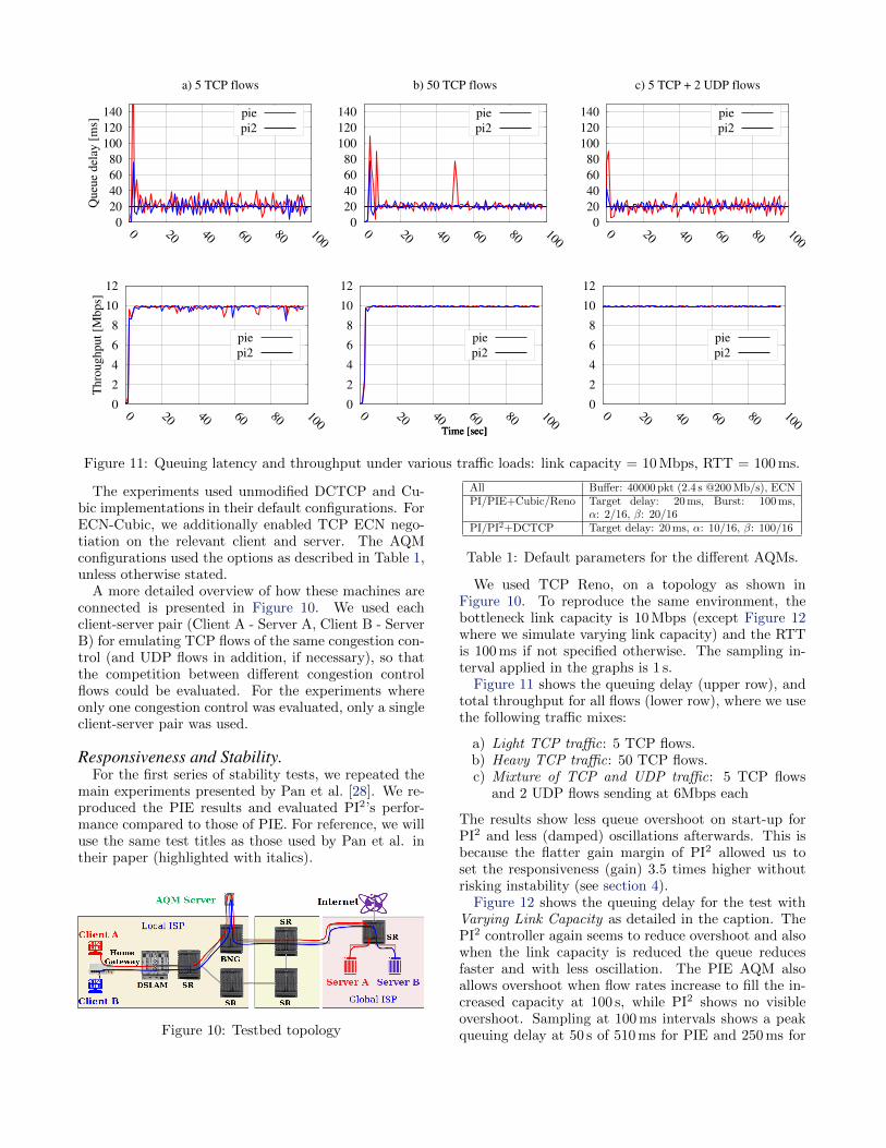
Figure 11 shows the queuing delay (upper row), andtotal throughput for all flows (lower row), where we usethe following traffic mixes:

a) Light TCP traffic: 5 TCP flows.b) Heavy TCP traffic: 50 TCP flows.c) Mixture of TCP and UDP traffic: 5 TCP flows

and 2 UDP flows sending at 6Mbps each

The results show less queue overshoot on start-up forPI2 and less (damped) oscillations afterwards. This isbecause the flatter gain margin of PI2 allowed us toset the responsiveness (gain) 3.5 times higher withoutrisking instability (see section 4).

Figure 12 shows the queuing delay for the test withVarying Link Capacity as detailed in the caption. ThePI2 controller again seems to reduce overshoot and alsowhen the link capacity is reduced the queue reducesfaster and with less oscillation. The PIE AQM alsoallows overshoot when flow rates increase to fill the in-creased capacity at 100 s, while PI2 shows no visibleovershoot. Sampling at 100 ms intervals shows a peakqueuing delay at 50 s of 510 ms for PIE and 250 ms for

0

50

100

150

200

250

0 20 40

60 80

100 120

140

Qu

eue

del

ay [

ms]

Time [sec]

pie

pi2

Figure 12: Performance comparison under varying linkcapacity: 100:20:100 Mb/s over durations 50:50:50 s

0

10

20

30

40

50

60

70

0 50 100

150 200

250

Queu

e del

ay [

ms]

Time [sec]

pie

pi2

Figure 13: Performance comparison under varying traf-fic intensity: 10:30:50:30:10 TCP flows over durations50:50:50:50:50 s, link capacity: 10 Mbps, RTT: 100 ms.

PI2. PIE has 2 more oscillation peaks above 100 msimmediately afterwards, while PI2 none at all.

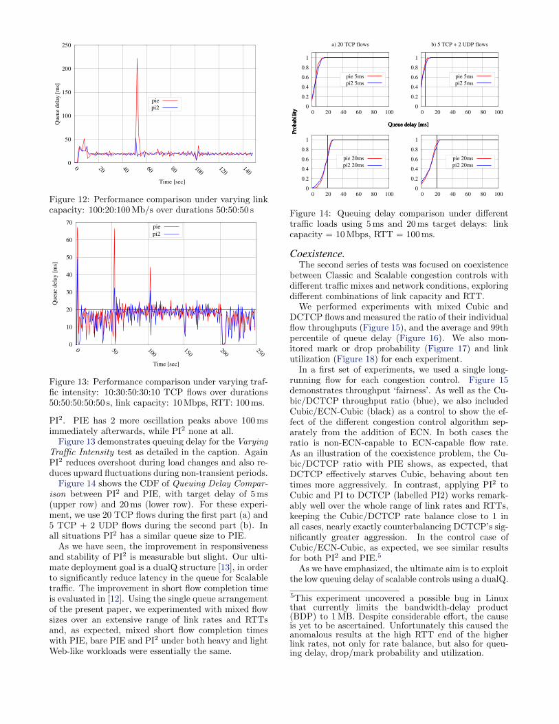
Figure 13 demonstrates queuing delay for the VaryingTraffic Intensity test as detailed in the caption. AgainPI2 reduces overshoot during load changes and also re-duces upward fluctuations during non-transient periods.

Figure 14 shows the CDF of Queuing Delay Compar-ison between PI2 and PIE, with target delay of 5 ms(upper row) and 20 ms (lower row). For these experi-ment, we use 20 TCP flows during the first part (a) and5 TCP + 2 UDP flows during the second part (b). Inall situations PI2 has a similar queue size to PIE.

As we have seen, the improvement in responsivenessand stability of PI2 is measurable but slight. Our ulti-mate deployment goal is a dualQ structure [13], in orderto significantly reduce latency in the queue for Scalabletraffic. The improvement in short flow completion timeis evaluated in [12]. Using the single queue arrangementof the present paper, we experimented with mixed flowsizes over an extensive range of link rates and RTTsand, as expected, mixed short flow completion timeswith PIE, bare PIE and PI2 under both heavy and lightWeb-like workloads were essentially the same.

0

0.2

0.4

0.6

0.8

1

0 20 40 60 80 100

a) 20 TCP flows

pie 5ms

pi2 5ms

Queue delay [ms]

Pro

bab

ilit

y

0

0.2

0.4

0.6

0.8

1

0 20 40 60 80 100

b) 5 TCP + 2 UDP flows

pie 5ms

pi2 5ms

Queue delay [ms]

Pro

bab

ilit

y

0

0.2

0.4

0.6

0.8

1

0 20 40 60 80 100

pie 20ms

pi2 20ms

Queue delay [ms]

Pro

bab

ilit

y

0

0.2

0.4

0.6

0.8

1

0 20 40 60 80 100

pie 20ms

pi2 20ms

Queue delay [ms]

Pro

bab

ilit

y

Figure 14: Queuing delay comparison under differenttraffic loads using 5 ms and 20 ms target delays: linkcapacity = 10 Mbps, RTT = 100 ms.

Coexistence.The second series of tests was focused on coexistence

between Classic and Scalable congestion controls withdifferent traffic mixes and network conditions, exploringdifferent combinations of link capacity and RTT.

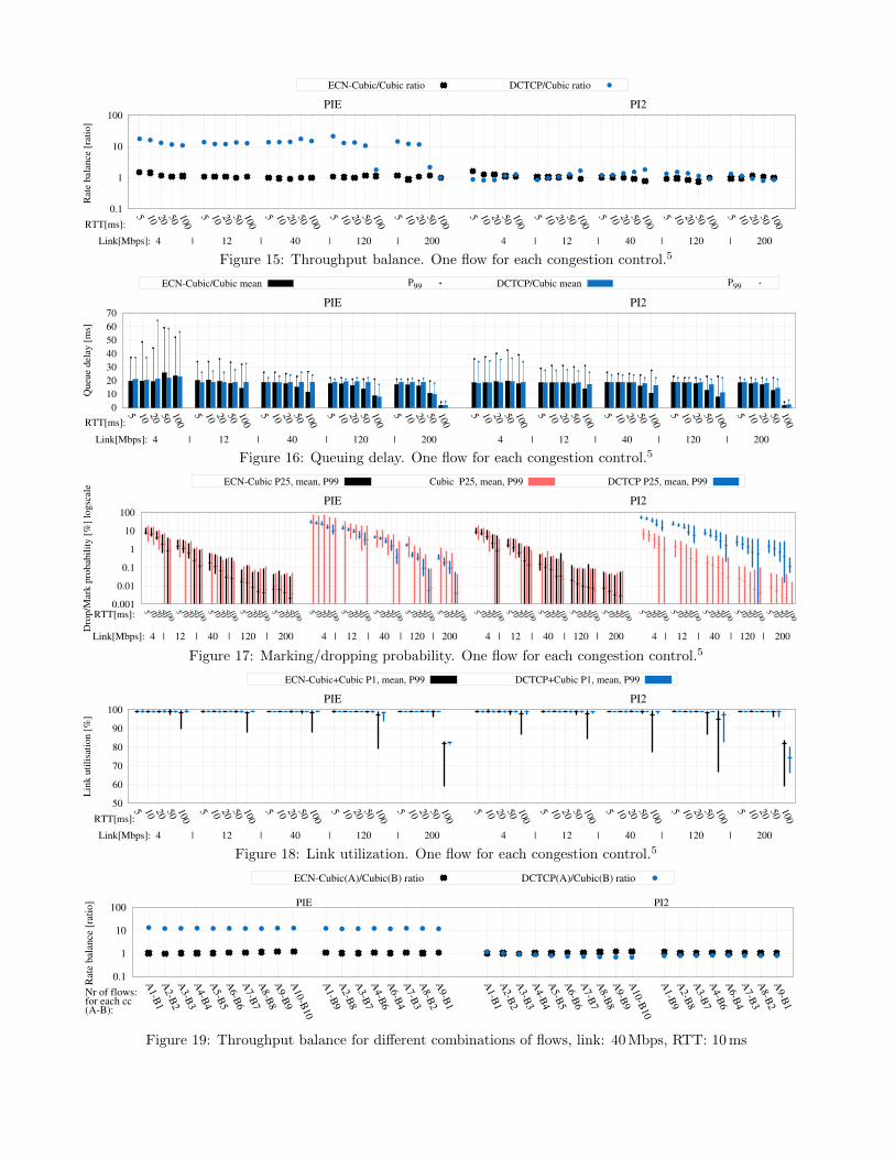
We performed experiments with mixed Cubic andDCTCP flows and measured the ratio of their individualflow throughputs (Figure 15), and the average and 99thpercentile of queue delay (Figure 16). We also mon-itored mark or drop probability (Figure 17) and linkutilization (Figure 18) for each experiment.

In a first set of experiments, we used a single long-running flow for each congestion control. Figure 15demonstrates throughput ‘fairness’. As well as the Cu-bic/DCTCP throughput ratio (blue), we also includedCubic/ECN-Cubic (black) as a control to show the ef-fect of the different congestion control algorithm sep-arately from the addition of ECN. In both cases theratio is non-ECN-capable to ECN-capable flow rate.As an illustration of the coexistence problem, the Cu-bic/DCTCP ratio with PIE shows, as expected, thatDCTCP effectively starves Cubic, behaving about tentimes more aggressively. In contrast, applying PI2 toCubic and PI to DCTCP (labelled PI2) works remark-ably well over the whole range of link rates and RTTs,keeping the Cubic/DCTCP rate balance close to 1 inall cases, nearly exactly counterbalancing DCTCP’s sig-nificantly greater aggression. In the control case ofCubic/ECN-Cubic, as expected, we see similar resultsfor both PI2 and PIE.5

As we have emphasized, the ultimate aim is to exploitthe low queuing delay of scalable controls using a dualQ.

5This experiment uncovered a possible bug in Linuxthat currently limits the bandwidth-delay product(BDP) to 1 MB. Despite considerable effort, the causeis yet to be ascertained. Unfortunately this caused theanomalous results at the high RTT end of the higherlink rates, not only for rate balance, but also for queu-ing delay, drop/mark probability and utilization.

0.1

1

10

100

5 10

20

50

100

5 10

20

50

100

5 10

20

50

100

5 10

20

50

100

5 10

20

50

100

5 10

20

50

100

5 10

20

50

100

5 10

20

50

100

5 10

20

50

100

5 10

20

50

100

Rat

e bal

ance

[ra

tio]

Link[Mbps]: 4 | 12 | 40 | 120 | 200 4 | 12 | 40 | 120 | 200

PIE PI2

ECN-Cubic/Cubic ratio DCTCP/Cubic ratio

RTT[ms]:

Figure 15: Throughput balance. One flow for each congestion control.5

0

10

20

30

40

50

60

70

5 10

20

50

100

5 10

20

50

100

5 10

20

50

100

5 10

20

50

100

5 10

20

50

100

5 10

20

50

100

5 10

20

50

100

5 10

20

50

100

5 10

20

50

100

5 10

20

50

100

Queu

e del

ay [

ms]

Link[Mbps]: 4 | 12 | 40 | 120 | 200 4 | 12 | 40 | 120 | 200

PIE PI2

ECN-Cubic/Cubic mean P99 DCTCP/Cubic mean P99

RTT[ms]:

Figure 16: Queuing delay. One flow for each congestion control.5

0.001

0.01

0.1

1

10

100

5 10

20

50

100

5 10

20

50

100

5 10

20

50

100

5 10

20

50

100

5 10

20

50

100

5 10

20

50

100

5 10

20

50

100

5 10

20

50

100

5 10

20

50

100

5 10

20

50

100

5 10

20

50

100

5 10

20

50

100

5 10

20

50

100

5 10

20

50

100

5 10

20

50

100

5 10

20

50

100

5 10

20

50

100

5 10

20

50

100

5 10

20

50

100

5 10

20

50

100

Dro

p/M

ark p

robab

ilit

y [

%]

logsc

ale

Link[Mbps]: 4 | 12 | 40 | 120 | 200 4 | 12 | 40 | 120 | 200 4 | 12 | 40 | 120 | 200 4 | 12 | 40 | 120 | 200

PIE PI2

ECN-Cubic P25, mean, P99 Cubic P25, mean, P99 DCTCP P25, mean, P99

RTT[ms]:

Figure 17: Marking/dropping probability. One flow for each congestion control.5

50

60

70

80

90

100

5 10

20

50

100

5 10

20

50

100

5 10

20

50

100

5 10

20

50

100

5 10

20

50

100

5 10

20

50

100

5 10

20

50

100

5 10

20

50

100

5 10

20

50

100

5 10

20

50

100

Lin

k u

tili

sati

on [

%]

Link[Mbps]: 4 | 12 | 40 | 120 | 200 4 | 12 | 40 | 120 | 200

PIE PI2

ECN-Cubic+Cubic P1, mean, P99 DCTCP+Cubic P1, mean, P99

RTT[ms]:

Figure 18: Link utilization. One flow for each congestion control.5

0.1

1

10

100

A1-B

1A

2-B

2A

3-B

3A

4-B

4A

5-B

5A

6-B

6A

7-B

7A

8-B

8A

9-B

9A

10-B

10

A1-B

9A

2-B

8A

3-B

7A

4-B

6A

6-B

4A

7-B

3A

8-B

2A

9-B

1

A1-B

1A

2-B

2A

3-B

3A

4-B

4A

5-B

5A

6-B

6A

7-B

7A

8-B

8A

9-B

9A

10-B

10

A1-B

9A

2-B

8A

3-B

7A

4-B

6A

6-B

4A

7-B

3A

8-B

2A

9-B

1

Rate

bala

nce [

rati

o] PIE PI2

ECN-Cubic(A)/Cubic(B) ratio DCTCP(A)/Cubic(B) ratio

Nr of flows:for each cc(A-B):

Figure 19: Throughput balance for different combinations of flows, link: 40 Mbps, RTT: 10 ms

0.01

0.1

1

10

A1-B

1A

2-B

2A

3-B

3A

4-B

4A

5-B

5A

6-B

6A

7-B

7A

8-B

8A

9-B

9A

10-B

10

A0-B

10

A1-B

9A

2-B

8A

3-B

7A

4-B

6A

6-B

4A

7-B

3A

8-B

2A

9-B

1A

10-B

0A

1-B

1A

2-B

2A

3-B

3A

4-B

4A

5-B

5A

6-B

6A

7-B

7A

8-B

8A

9-B

9A

10-B

10

A0-B

10

A1-B

9A

2-B

8A

3-B

7A

4-B

6A

6-B

4A

7-B

3A

8-B

2A

9-B

1A

10-B

0A

1-B

1A

2-B

2A

3-B

3A

4-B

4A

5-B

5A

6-B

6A

7-B

7A

8-B

8A

9-B

9A

10-B

10

A0-B

10

A1-B

9A

2-B

8A

3-B

7A

4-B

6A

6-B

4A

7-B

3A

8-B

2A

9-B

1A

10-B

0A

1-B

1A

2-B

2A

3-B

3A

4-B

4A

5-B

5A

6-B

6A

7-B

7A

8-B

8A

9-B

9A

10-B

10

A0-B

10

A1-B

9A

2-B

8A

3-B

7A

4-B

6A

6-B

4A

7-B

3A

8-B

2A

9-B

1A

10-B

0

No

rmali

sed

rate

PIE PI2

ECN-Cubic(A) P1, mean, P99 Cubic (B) P1, mean, P99 DCTCP(A) P1, mean, P99

Nr of flows:for each cc(A-B):

Figure 20: Throughput stability shown as normalized rate per flow (rate per flow divided by ‘fair’ rate) for differentcombinations of flows, link: 40 Mbps, RTT: 10 ms

With the single-queue approach studied in this paper,the queuing delay experienced by each type of concur-rent flow had to be the same. In Figure 16 we comparethe average and 99th %-ile (P99) of queue delay for eachpacket between the two scenarios: a Cubic flow with anECN-Cubic or a DCTCP flow. As expected, there islittle difference between the scenarios. Nonetheless, theresults indicate that PI2 appears to be no worse thanPIE at keeping the queue delay at the target of 20ms.PI2 even seems to outperform PIE at smaller link rates,which can be seen at the link rate of 4Mbps, where P99

is larger for PIE.To verify whether the throughput ratio is influenced

by the number of concurrent flows, we tested it with arange of combinations of flow numbers. Figure 19 showsthe per-flow throughput ratio for the combinations offlows displayed on the x-axis, where each combinationis represented by two numbers. The first is the num-ber of Cubic flows, while the second is the number ofECN-Cubic or DCTCP flows respectively. The resultswere similar for different link capacities and RTTs, sowe show results for a link capacity of 40 Mbps and 10 msRTT as an example. Figure 20 visualizes the same ex-periment, but includes the mean and %-iles by showingnormalized rates. The results are very similar to thosein Figure 15 showing that PI2 can maintain equal flowrates irrespective of the number of concurrent flows.

7. CONCLUSIONSThe main conclusions of this work are twofold.

Firstly, despite PI2 being simpler than PIE, it achievesno worse, and in some cases better performance, partic-ularly superior responsiveness during dynamics withoutrisking instability. This has been demonstrated bothanalytically and through a number of experiments. Inother words, the heuristic scaling steps introduced byPIE can be replaced by squaring the output instead,which is less computationally expensive and improvesstability in some cases.

Secondly, in contrast to PIE, a combination of PI andPI2 can support coexistence of Scalable and Classic con-gestion controls on the public Internet by counterbal-ancing the more aggressive congestion response of Scal-able controls with more aggressive congestion marking.It has been emphasized throughout that the arrange-

ment of both PI and PI2 in the same queue evaluatedin this paper is only a step in the research process, not arecommended deployment. The recommended deploy-ment applies each AQM to separate queues [13] so thatScalable traffic in the PI-controlled queue can maintainextremely low latency while isolated from but coupledto the queue built by Classic traffic controlled by PI2. Acomplementary paper explains and evaluates this ‘Du-alQ Coupled’ approach [12].

AcknowledgementThe authors’ contributions were part-funded by the Eu-ropean Community under its Seventh Framework Pro-gramme through the Reducing Internet Transport La-tency (RITE) project (ICT-317700). The views ex-pressed here are solely those of the authors.

APPENDIXA. EQUAL STEADY STATE RATE

Classic TCPs have a throughput equation that is pro-portional to the square root of the signal probability.For our purposes, it is sufficient to ignore dynamic as-pects, and apply the simplified models in (5) and (6)for TCP Reno and Cubic window as in [25] and [16]:

Wreno =1.22

p1/2(5) Wcubic =

1.17R3/4

p3/4(6)

where p is drop probabillity and R is the RTT.As we said, the Cubic implementation in Linux falls

back to TCP Reno with a different decrease factor (B =0.7 in Linux), thus the CReno steady state window willdeviate from (5) with a slightly higher constant (7).

The implicit switch-over RTT can be derived from (6)and (7). Pure Cubic behaviour (as defined in (6)) willbecome active when (8) is false.

Wcreno =1.68

p1/2(7) W ∗R3/2 < 3.5 (8)

This shows that the switch-over point does not de-pend on a single RTT or BDP (bandwidth delay prod-uct) value, but a more complex combination of RTTand window (W ).

In this paper we focus on fairness between Scalableflows and Cubic flows in their Reno mode (CReno). For

the Scalable TCP we use DCTCP with probabilistic(not on-off) marking applied by the AQM. We have de-rived the steady-state window equation for DCTCP inthis case, assuming an idealized uniform deterministicmarker, which marks every 1/p packets. A DCTCP con-gestion controller has an incremental window increaseper RTT a = 1 and a multiplicative decrease factorb = p/2 (with p being estimated). So, every RTT, W isincreased by W ← W + 1, meaning that under steadystate, this must be compensated every RTT by (9). Thisdecrease is steered by ECN marks, as defined in (10).

W ←(

1− 1

W

)W (9) W ←

(1− p

2

)W (10)

From (9) and (10), we see that to preserve this bal-ance, window equation (11) must be true.

Wdc =2

p(11) Wdcth =

2

p2(12)

Note that (12) derived in the DCTCP paper [2] hasa different exponent of p compared to (11). The reasonis that (12) is defined for a step threshold, which causesan on-off pattern of RTT length marking trains. Incontrast, when marking for DCTCP is steered by a PIcontroller, its random process with a fractional proba-bility will cause an evenly distributed marking pattern,so (11) will be applicable. This explains the same phe-nomenon found empirically in Irteza et al [22], whencomparing a step threshold with a RED ramp.

A Scalable congestion controller such as DCTCPachieves low throughput variations by driving the net-work to give it a more responsive signal with a higherresolution. Therefore, a solution must be found to re-duce the congestion signal intensity for Classic conges-tion controllers (TCP Cubic and Reno), balanced withthat for DCTCP.

Knowing the relation between network congestion sig-nal (mark or drop) probability and window, we can ad-just feedback from the network to each type of conges-tion control. For TCP CReno and DCTCP, we substi-tute (7) and (11) in Wcreno = Wdc:

1.68

p1/2creno

=2

pdc(13) pcreno =

( pdc1.19

)2

(14)

Therefore, if the RTTs are equal, we can arrange therates to be equal using the simple relation between theprobabilities, defined in (14).

Probabilistic mark/drop is typically implemented bycomparing the probability p with a pseudo-randomlygenerated value Y per packet. A signal is applied fora packet when Y < p. The advantage of using rela-tion (14) is that p2 can easily be acquired by compar-ing p with 2 pseudo-random generated values and sig-nalling only if both random values are smaller than p:max(Y1, Y2) < p.

The phrase“Think once to mark, think twice to drop”is a useful aide-memoire for this approach, because Scal-able controls always uses ECN marking (the markinglevel is often too high to use drop), while Classic con-trols typically use drop.

B. FLUID MODELIn Pan et al [29] a PIE controller was designed for

TCP Reno. TCP Reno has a throughput that is pro-portional to 1/

√p. In this analytical section we define

first a model for a system that has an adaptor on theoutput of the controller that squares the signal, so thecontroller generates a signal p′ =

√p which is finally

applied to the packets as a marking or dropping signalp = (p′)2.

Secondly we define a system where the TCP is definedas a so-called scalable congestion control (section 2)with a throughput that is proportional to 1/p′, so nosquaring is needed at the end. We will consistently usep′ to indicate a scalable probability and p to indicate aclassic probability. One can be derived from the otherwith the above equation.

We start from the model of the evolution of the win-dow of TCP Reno and the dynamics of the queue fromMisra et al [26] and [19]:

dW (t)

dt=

1

R(t)− 0.5

W (t)W (t−R(t))

R(t−R(t))p(t−R(t)),

(15)

dq(t)

dt=W (t)

R(t)N(t)− C(t), (16)

where W (t) is the window size, q(t) the queue size, R(t)the harmonic mean of the round trip time of the differ-ent flows, N(t) is the number of flows, and C(t) is thelink capacity, which might also vary over time, but ishere assumed independent from all other variables.

The Cubic implementation in Linux provides a fall-back to TCP Reno when RTT or rate is small (CReno).For CReno mode the multiplicative reduction factor is0.7 instead of 0.5, which results in an equation that isjust slightly different:

dW (t)

dt=

1

R(t)− 0.7

W (t)W (t−R(t))

R(t−R(t))p(t−R(t)).

(17)

For TCP Reno that is steered by a squared probabil-ity, the following equation is used to derive the transferfunction:

dW (t)

dt=

1

R(t)− 0.5

W (t)W (t−R(t))

R(t−R(t))

(p′(t−R(t))

)2.

(18)

Doing the similar linearization exercise for (18) asfor (15) in [19], assuming for now N(t) = N , C(t) =C, R(t) = R0 as constants, we get operating pointequations (defined by dW/dt = 0, dq/dt = 0 and

(W, q, p′) = (W0, q0, p′0)):

W 20 p′20 = 2, W0 =

R0C

N, R0 =

q0C

+ Tp, (19)

where Tp is the base delay of a specific flow.The partial derivations are the same as in Appendix

I of [19] except:

∂f

∂p′= −W

20

2R02p′0 = −

√2C

N,

where f(W,WR, q, p′) is defined as the RHS of Equa-

tion 18, and WR = W (t−R). Note that

∂f

∂W=

∂f

∂WR=−W0

2R0p′20 =

−W0

2R0

2

W 20

=−1

R0W0=−NR2

0C,

∂f

∂q= − 1

R20C

+W 2

0 p′20

2R20C

= − 1

R20C

+2

2R20C

= 0,

both of which initially have different terms to the anal-ysis in [19], but eventually resolve to the same resultas [19]. As a result, the linearized equation for a RenoTCP with a squared p′ and its Laplace transform willbe:

d(δW (t))

dt= − N

R20C

(δW (t) + δWR)−√

2C

Nδp′(t−R0);

(20)

sW (s) = − N

R20C

W (s)(1 + e−sR0)−√

2C

Np′(s)e−sR0 .

(21)

Also for a scalable TCP that reduces its current win-dow by half a packet per mark, the following equationcan be derived in a similar way:

dW (t)

dt=

1

R(t)− 0.5

W (t−R(t))

R(t−R(t))p′(t−R(t)). (22)

The difference is that the current window size W (t) isnot present as it is not used to determine the windowreduction. This makes the reduction term only depen-dent on the state at time t−R(t).

Re-running the linearization exercise for (22) as in[19], we get operating point equations:

W0p′0 = 2, W0 =

R0C

N, R0 =

q0C

+ Tp. (23)

The partial derivations are the same as in [19] exceptfor:

∂f

∂W= 0;

∂f

∂p′= −W0

2R0= − C

2N.

Note that

∂f

∂WR= − 1

2R0p′0 = − 1

2R0

2

W0= − 1

R0W0= − N

R20C

,

which initially had different terms to the analysis in [19],but eventually resolves to the same result as [19]. As aresult, the linearized equations for a scalable TCP and

its Laplace transform will be:

d(δW (t))

dt= − N

R20C

δW (t−R0)− C

2Nδp′(t−R0);

(24)

sW (s) = −e−sR0( N

R20C

W (s)− C

2Np′(s)

). (25)

From [26] and [19] we repeat the linearized queueequation, its Laplace transform and Laplace transferfunction:

d(δq(t))

dt=

N

R0δW (t)− 1

R0δq(t); (26)

sq(s) =N

R0W (s)− 1

R0q(s), (27)

Pqueue(s) =q(s)

W (s)=

NR0

s+ 1R0

. (28)

The PI transfer function in the Laplace domain is:

CPI(s) =β+α/2C s+ α

TC

s. (29)

The combined PI and queue (=AQM) transfer functionin terms of R0 and W0 is:

A(s) =(β + α

2 )s+ αT

s

1W0

s+ 1R0

, (30)

A(s) =κAW0

(s/zA + 1)

s(s/sA + 1), (31)

with κA = αR0/T , zA = α/(T (β + α/2)) and sA =1/R0.

The transfer functions of the different TCP and mark-ing combinations in terms of W0, R0 and p0 or p′0 are:

Prenop(s) =W (s)

p(s)= − W0κRe

−sR0

s/sR + (1 + e−sR0)/2; (32)

Prenop′2 (s) =W (s)

p′(s)= − W0κSe

−sR0

s/sR + (1 + e−sR0)/2; (33)

Pscalp′ (s) =W (s)

p′(s)= − W0κSe

−sR0

s/sS + e−sR0, (34)

with κS = 1/p′0, sS = p′0/(2R0), κR = 1/(2p0) = κ2S/2

and sR =√

2p′0/R0 =√

2p0/R0 =√

8sS .The complete loop transfer functions are:

Lrenop(s) =κRκA(s/zA + 1)e−sR0

(s/sR + (1 + e−sR0)/2)(s/sA + 1)s;

(35)

Lrenop′2 (s) =κSκA(s/zA + 1)e−sR0

(s/sR + (1 + e−sR0)/2)(s/sA + 1)s;

(36)

Lscalp′ (s) =κSκA(s/zA + 1)e−sR0

(s/sS + e−sR0)(s/sA + 1)s. (37)

8. REFERENCES[1] R. Adams. Active Queue Management: A Survey.

IEEE Communications Surveys & Tutorials,15(3):1425–1476, 2013.

[2] M. Alizadeh, A. Greenberg, D. A. Maltz,J. Padhye, P. Patel, B. Prabhakar, S. Sengupta,and M. Sridharan. Data Center TCP (DCTCP).Proc. ACM SIGCOMM’10, ComputerCommunication Review, 40(4):63–74, Oct. 2010.

[3] M. Alizadeh, A. Javanmard, and B. Prabhakar.Analysis of DCTCP: Stability, Convergence, andFairness. In Proceedings of the ACMSIGMETRICS Joint International Conference onMeasurement and Modeling of Computer Systems,SIGMETRICS ’11, pages 73–84, New York, NY,USA, 2011. ACM.

[4] D. Black. Explicit Congestion Notification (ECN)Experimentation. Internet Draftdraft-black-tsvwg-ecn-experimentation-00,Internet Engineering Task Force, Sept. 2016.(Work in Progress).

[5] O. Bondarenko, K. De Schepper, I.-J. Tsang,B. Briscoe, A. Petlund, and C. Griwodz.Ultra-Low Delay for All: Live Experience, LiveAnalysis. In Proc. ACM Multimedia Systems;Demo Session, pages 33:1–33:4. ACM, May 2016.

[6] B. Briscoe. Review: Proportional Integralcontroller Enhanced (PIE) Active QueueManagement (AQM). Technical ReportTR-TUB8-2015-001, BT, May 2015.

[7] B. Briscoe, A. Brunstrom, A. Petlund, D. Hayes,D. Ros, I.-J. Tsang, S. Gjessing, G. Fairhurst,C. Griwodz, and M. Welzl. Reducing InternetLatency: A Survey of Techniques and theirMerits. IEEE Communications Surveys &Tutorials, 18(3):2149–2196, 2016.

[8] B. Briscoe (Ed.), K. De Schepper, andM. Bagnulo. Low Latency, Low Loss, ScalableThroughput (L4S) Internet Service: ProblemStatement. Internet Draft draft-briscoe-tsvwg-aqm-tcpm-rmcat-l4s-problem-02, InternetEngineering Task Force, July 2016. (Work inProgress).

[9] CableLabs. Data-Over-Cable Service InterfaceSpecifications DOCSIS R© 3.1; MAC and UpperLayer Protocols Interface Specification.Specification CM-SP-MULPIv3.1-I01-131029,CableLabs, Oct. 2013.

[10] Y. Choi, J. A. Silvester, and H.-c. Kim. Analyzingand Modeling Workload Characteristics in aMultiservice IP Network. Internet Computing,IEEE, 15(2):35–42, March 2011.

[11] K. De Schepper and O. Bondarenko. Linuxsch pi2 qdisc source code available athttps://github.com/olgabo/dualpi2, June 2016.

[12] K. De Schepper, O. Bondarenko, I.-J. Tsang, andB. Briscoe. ‘Data Centre to the Home’:

Deployable Ultra-Low Queuing Delay for All.Sept. 2016. (Under Submission).

[13] K. De Schepper, B. Briscoe (Ed.), O. Bondarenko,and I.-J. Tsang. DualQ Coupled AQM for LowLatency, Low Loss and Scalable Throughput.Internet Draftdraft-briscoe-aqm-dualq-coupled-01, InternetEngineering Task Force, Mar. 2016. (Work inProgress).

[14] K. De Schepper, B. Briscoe (Ed.), and I.-J.Tsang. Identifying Modified Explicit CongestionNotification (ECN) Semantics for Ultra-LowQueuing Delay. Internet Draftdraft-briscoe-tsvwg-ecn-l4s-id-01, InternetEngineering Task Force, Mar. 2016. (Work inProgress).

[15] N. Finn (Ed.). IEEE Standard for Local andMetropolitan Area Networks—Virtual BridgedLocal Area Networks - Amendment: 10:Congestion Notification. Standard 802.1Qau,IEEE, Apr. 2010.

[16] S. Ha, I. Rhee, and L. Xu. CUBIC: a newTCP-friendly high-speed TCP variant. SIGOPSOperating Systems Review, 42(5):64–74, July2008.

[17] O. Hohlfeld, E. Pujol, F. Ciucu, A. Feldmann,and P. Barford. A QoE Perspective on SizingNetwork Buffers. In Proc. Internet MeasurementConf (IMC’14), pages 333–346. ACM, Nov. 2014.

[18] C. V. Hollot, V. Misra, D. Towsley, and W. Gong.Analysis and design of controllers for AQMrouters supporting TCP flows. IEEE Transactionson Automatic Control, 47(6):945–959, Jun 2002.

[19] C. V. Hollot, V. Misra, D. F. Towsley, andW. Gong. A Control Theoretic Analysis of RED.In Proc. INFOCOM 2001. 20th Annual JointConf. of the IEEE Computer andCommunications Societies., volume 3, pages1510—19, 2001.

[20] Y. Hong and O. W. W. Yang. Self-tuning TCPtraffic controller using gain margin specification.IET Communications, 1(1):27–33, February 2007.

[21] Y. Hong, O. W. W. Yang, and C. Huang.Self-tuning PI TCP flow controller for AQMrouters with interval gain and phase marginassignment. In Global TelecommunicationsConference (Globecom’04), volume 3, pages1324–1328, 2004.

[22] S. Irteza, A. Ahmed, S. Farrukh, B. Memon, andI. Qazi. On the Coexistence of TransportProtocols in Data Centers. In Proc. IEEE Int’lConf. on Communications (ICC 2014), pages3203–3208, June 2014.

[23] M. Kuhlewind, D. P. Wagner, J. M. R. Espinosa,and B. Briscoe. Using Data Center TCP(DCTCP) in the Internet. In Proc. Third IEEEGlobecom Workshop on Telecommunications

Standards: From Research to Standards, pages583–588, Dec. 2014.

[24] M. Kwon and S. Fahmy. A Comparison ofLoad-based and Queue-based Active QueueManagement Algorithms. In Proc. Int’l Soc. forOptical Engineering (SPIE), volume 4866, pages35–46, 2002.

[25] M. Mathis, J. Semke, J. Mahdavi, and T. Ott.The macroscopic behavior of the TCP CongestionAvoidance algorithm. Computer CommunicationReview, 27(3), July 1997.

[26] V. Misra, W.-B. Gong, and D. Towsley.Fluid-based Analysis of a Network of AQMRouters Supporting TCP Flows with anApplication to RED. SIGCOMM ComputerComms.. Review, 30(4):151–160, Aug. 2000.

[27] K. Nichols and V. Jacobson. Controlling queuedelay. ACM Queue, 10(5), May 2012.

[28] R. Pan et al. PIE: A lightweight control scheme toaddress the bufferbloat problem. In Proc. IEEEInt’l Conf. on High Performance Switching andRouting (HPSR), pages 148–155, 2013.

[29] R. Pan, P. Natarajan, F. Baker, G. White,B. Ver Steeg, M. Prabhu, C. Piglione, andV. Subramanian. PIE: A Lightweight ControlScheme To Address the Bufferbloat Problem.Internet Draft draft-ietf-aqm-pie-10, InternetEngineering Task Force, Sept. 2016. (Work inprogress).

[30] K. K. Ramakrishnan, S. Floyd, and D. Black. TheAddition of Explicit Congestion Notification(ECN) to IP. Request for Comments RFC 3168,RFC Editor, Sept. 2001.

[31] M. Sagfors, R. Ludwig, M. Meyer, and J. Peisa.Buffer Management for Rate-Varying 3G WirelessLinks Supporting TCP Traffic. In Proc VehicularTechnology Conference, Apr. 2003.

[32] G. White. Active Queue Management Algorithmsfor DOCSIS 3.0; A Simulation Study of CoDel,SFQ-CoDel and PIE in DOCSIS 3.0 Networks.Technical report, CableLabs, Apr. 2013.