PI THE VIRIAL TENSOR EQUATIONS BY

EUGENE N. PARKER

TECHNICAL REPORT NO. 1

January 1, 1954

EARTH'S MAGNETISM AND MAGNETOHYDRODYNAMICS

CONTRACT Now 1288(00)

OFFICE OF NAVAL RESEARCH

DEPARTMENT OF PHYSICS

UNIVERSITY OF UTAH

SALT LAKE CITY

THE TENSOR VIRIAL EQUATIONS-''"

Eugene N. Parker

Department of Physics

University of Utah

Salt Lake City, Utah

Abstract

The tensor virial equations of notion are developed. They

are found to be tensor equations of second rank which upon

contraction give the usual scalar virial equation. The tensor

virial equations may be applied to anisotropic systems in the same

manner that the scalar virial equation is anplied to isotropic

systems. Several applications of the tensor virial equations

are considered. The diffusion of ions through a magnetic field

and the diffusion of molecules through a gas are calculated.

The derivation of the Navier - Stokes eqijations and the Reynolds

stress tensor for a turbulent flow is developed, leading in a

natural wav to Prandtl's mixing lenrth ideas. The dynamics of a

self gravitating oscillating gas cloud is investigated. The

expressions for gravitating homogeneous elliosoidal regions are

worked out for use in oroblems involving inverse square inter-

actions, e.f„ galactic dynamics, clouds of charged oarticles , etc.

Because of the aoolicabilitv to hydromagnetics, the stress tensor

formulation of the tensor virial equations is developed in the

last section.

••n»w. -'» '""•- *J '.IJI- ;'" ••»•„'•» •' :.:oA^'^^^^-;-MI&^'^ jj.lC.-ll 111 jjjll «.•» I « !• Il-I-I

Introduction

0.1 The use of the virial theorem in kinetic theory is well

known. It does not seem to have been remarked with sufficient

generality that the virial equation can be extended to a set of

equations between tensor components. A3 the formulas of the

first section show, these relations ai e essential]y equations of

motion for the ordinary moment of inertia tensor of an assembly

of particles. The usual scalar virial theorem results from the

tensor equations bv the process of contraction. The tensor

virial equations are useful in problems of the dynamics of complex

systems, especially in hydrodynamics and transport theory where

the actual integration of the equations of motion is not practical.

One may then obtain approximate information by investigating

the behavior of the moment of inertia of the system or of a

subsystem, e.g. an eddy. The tensor form of the equations permits

one to obtain results for anisotropic motions wherever the scalar

virial can he applied to isotropic motions.

The method hrs oroved useful in astronhysical problems,

particularly those dealing with the dynamics of a finite region,

e.g. the dynamics of an individual star, clusters of stars, and

"alaxies '. We shall treat some illustrative examples in trans-

nort theory. We shall find that the main advantage will ^e a

means of sidestepping uninteresting detail, such as the precise

densitv distribution, allowing one to compute directly the more

pertinent quantities, e.g. mean diffusion or expansion rates,

mean pressures and viscous stresses etc.

We shall derive the Navier - Stokes equations from the tensor

i

IV

.

I ' »!•»•. »-> IIP! II >|.«l'» .-^jLwmf" 8B5JWMWaH»" •' •"' '•"

a»J -**". i - m*eaaam»anm

i jt

dflj

£"* : >», •

... 2

viriai equations and show that the oarallelism of viscous and Jf., "- Mi- : -- •

SK' _ -

turbulent stresses is inherent in the theory without any

artificiality. Thus, it forms a basis for the turbulence theories

to be found elsewhere'~a. The generality of our results makes them . S - • ---

applicable to the construction of a statistical magnetohydrodynamic >»•, >•>,<• JT _. » . •

theory of the same nature as existing turbulence theories.

It is well known that the scalar viriai theorem holds "in"

quantum mechanics*, an extension of the tensor viriai theorem

to the quantum mechanical case should be oossible , but will not

be attempted here.

'V:

V— - -ar5£*--*. ~\.r-jr-^*-

. —.-~Wt&#^*^~

^ —-•*•

-- . * t •

9 ><

^&-i

i - »

eaa ta --.^jiHfgr^int^g^^-v i IJIWJU mini ,4K

3**m dh UlfcwMMKlrfWM^I^ <*i, „. ^ *>$ <« ^ - 11.»'.»-J ' '">'

ft j j I

Lagrangisn Formulation

1.1 Consider a system of particles in a space with the cartesian

coordinates x . We shall for the moment fix our attention on

the vth particle. We represent its mass bv m and its position v bv x . We assume that all velocities are small C">mt>ared to the

i *

sriecd of lipht. The Lagrangian is written

L = T - V v v v where T and V represent the kinetic and ootential energies,

(1)

Let us introduce the svmbol Q, to denote those forces for

which a scalar potential does not exist. In this category we

include all forces of constraint. The Q. are defined as the v 1

differential coefficients in the expression for the wbrlc

8 w = Q,<6 x1 v v i v (2)

Repeated italic indices irmly summation convention; Greek do not.

The b x represent an arbitrary displacement of the vth particle

under the effect of all those forces not included in V. v Lagrange's equations for the vth particle become

V

TxX V

n

Multiplying by x'-' gives us the tensor equation of second rank

which riav he written as

d dt

XJ V

(v - V

3 L V + x'!

V

3 L V

3 £i vA 3 xl

V

+ V*' V^i (4;

-• i

3!

I Consider now the sum over a number of particles in the

space. We shall indicate the summation by In practice this

sum is usually effected by summing over all particles in a simply

connected region of space, though in some diffusion problems

• 4W&M**-

tgH%fatomm*&ai*l&tlllfi&*0 ' . '• 9 i " g*g

(cf. 2.12) this Is not the case. We define the tensors

i i *— v -5—rf ••' v o x7

v

2Ti.i= ?/' ^ v TV V

v T1F

(5)

(6)

(7)

1' * i

••'••

An- x1 3L " _

and the scalars .

-SI L v v

8)

(9)

T =

V = V

(10)

(11)

Thus, L, T, and V are the Lagrangian, kinetic energy, and potential

energy respectively of the particles over which we are sunning.

(4) may be rewritten as

d _ dt V 2Tij+ * ij +p-ij (12)

These tensors admit of a straight forward internretation.

The diagonal components of J, , are -just J..1

f

•

i -

i 1

.:*i •*l

*| • 3! c

V •'-

ra©»3Ba«W! Wvimyptfj" iB|ai».#ww6=^«-'

fl& jsn m i T • •—

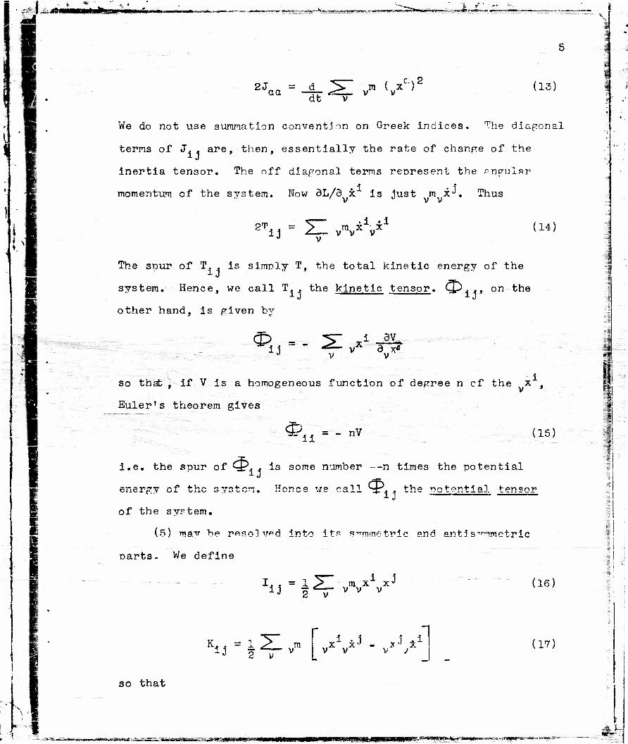
2J aa •4S dt

/ cN2 vm (vx ) (13)

We do not use summation convention on Greek indices, ^he diagonal

terns of J. , are, then, essentially the rate of change of the

inertia tensor. The off diagonal terms represent the p.npulnr

momentum of the system. Now 3L/3 x"1" is iust m xJ. Thus ' v J V V

\

!>•

1

2T ij vVV* (14)

The spur of T. , is simply T, the total kinetic energy of the

system. Hence, we call T. . the kinetic tensor. CD. ., on the

other hand, is given by

5" x1 -2L T*v 8v^

so that , if V is a homogeneous function of degree n cf the x t

Euler's theorem gives

<%, = - nV (15)

i.e. the spur of <$*, . is some number --n times the potential

energy of the system. Hence we call SP. , the potential tensor

of the system.

(5) may be resolved into it-*3 P^TTimetric £>nd antj s'^metric

parts. We define

"ij f 2 v m X x**

v v v (16)

K<< - 1 ij .m

2 v x X'1' - X^ X

V V V J .A (17)

so that

• E- —•IIIPIII imn—saiBWi Fthi—m%iaT.r~-'•It-**'liMII llttTr' "^WW tfE^WWwfcr^*

TM ^*j.ll. • . -'-^1

dt ~ij I., = 1 (J,4 + J.,) ij .li- ds)

i

Further, we let

K ij

= 1 U, , - J.J t "U Ji'

Ti^l^. + cjp..

ij = 1 <ft. _ <£t

M, , = 1 ^[A^ Ni3=i

Thus we have the symmetric and anti-symmetric equations

/.

(19)

(20)

(21)

(22)

(23)

—c- I = 2T + T + M dt2

1ij _^13 + I ij + nij (24)

*

d dt Wij -ij 'ij

(25)

The symmetric equation gives the manner in which the moment

of inertia tensor, I**, varies. The antisymmetric equation gives

the rate of change of the angular momentum K. . of the region.

It is well known that if the interaction of the narticles

mav be ex-Dressed in terms of central force fields, they c'o not

transfer angular momentum. Hence, in the absence of external

fields we have

— ij = HU = ° (26)

I

T^^wttsammKm*2wmtm*mmmmmmsmBmti$Mammfm i< .^wei,ll'»"" •^^^^WP*^1'^*11.11111 " " •"• ,_ =«— « Sfe

•^^d.- —..fa.... I- r

,7

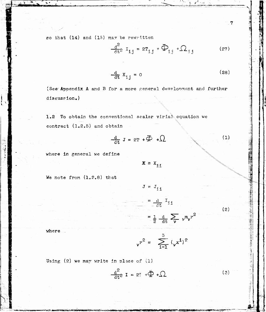
so that (14) and (15) may be rewritten p

dtd ij ij •*«, +-ft«. ij i J

K. . = 0

(27)

(28) dt ij

(See' Appendix A and B for a more general development and further

discussion.)

1.2 To obtain the conventional scalar virial equation we

\

II

\

contract (1.2.5) and obtain

dt J = 2T +<^ +11 (1)

where in general we define

We note from (1.2.8) that

X £ X ii

I

X

J = J. ii

= a

= 1 d

"ii

(2)

2 dt v m 3 v v

where

i

H 1

ii .:

/= si^2

l i

Using (2) we ma:'' write in place of (1)

(3)

fc

»»**••-»« r^nevKMnHnoi ;.- ,,yfcj^fcaiai6^saj.aBSiraJA»fi-^»!r?-*J-'

f*m*mmm*m i ..'» ml—JO-asr-

8

Aoplicatior. s

I i

i

2,1 It will be our purpose in this section to illustrate some of

the methods of application of the tensor virial equations to

transport problems and associated kinetic nhenomena.

»•

.

!'

2.11 Consider a simply connected cloud of electrons and protons

in a uniform magnetic field. We assume that the net ch.qrge of

the cloud is zero and recombination is negligible. The Lagrangian

for the vth oarticle is

L = 1 m. v v* + vq

£ v v v A1 v1 V V (1)

where A is the vector potential representing the magnetic field,

q the charge. It follows that

3„L 3 vi v

= V V i q . i m vx + vH ..A - v

!

-a

3 x-1- c 3 x* v v

~2Jm£L**»- -

We obtain from (1.1.12), after some rearranging

d <«-— i -dt ^L vmvv v

**

.1XJ i 1 q wm v vJ - xJv/* v v v v -*- c dt ' Sx1

~) (2)

J If we assume the magnetic field to be of magnitude B and

in the positive z direction, then we may take

K = -I By, A = 1 Bx, A = o, aAj_ = o (3) at

Thus, we obtain the three equations

Hi

f!

£

TT—r

!.*• • mm

.m v x^ = dt v v xv (. e

ra v v1 + v v xv • 0 _JL v B

C V V

9

(4)

I 4

-rr ^ m V XJ = dt •c^~ v v yv

dt ^_ v*W,xJ =

1 m v v*' - x*' ,v v yv v v B V X

vmvvzvv i

(5)

(6)

Summing over the whole cloud the off diagonal terms average out

because there is no correlation between v , and v% or x and x^. V ' V ' V V '

(i ^ j) as we sum over v. We are left with the diagonal terms

d dt

_d dt

„m v x = v v xv

vravvyvy =

v»W + S v v y j

(7)

r,ra( v )2 - vq y v B~j <v v y —~ vJv x J (8)

•

1:

d dt vmvvzvz m( v )2

v v z (9)

i

We see from (9) that we have free expansion in the z direction.

Consider (7). We must compute ^> a x v B/c. We shall v v v y '

describe the average position of a oarticle between successive

collisions by means of the center of mass of its trajectory. The

projection on the xy plane of the velocity is

vvxy=vGx)2 +(vv2 (io)

! ;

- •

B

The radius of curvature of the nro lection on the xy olane is

(ID

$1

TT"

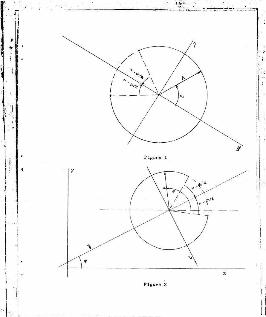
•*•• n4i -A* ,titin *nti**\ titoUiwm iwwh-- LU>J*W I i iffci jWiwifaW»a-^-^gSfe .iiMT." "-"fcr-i^i'dfc ] 10

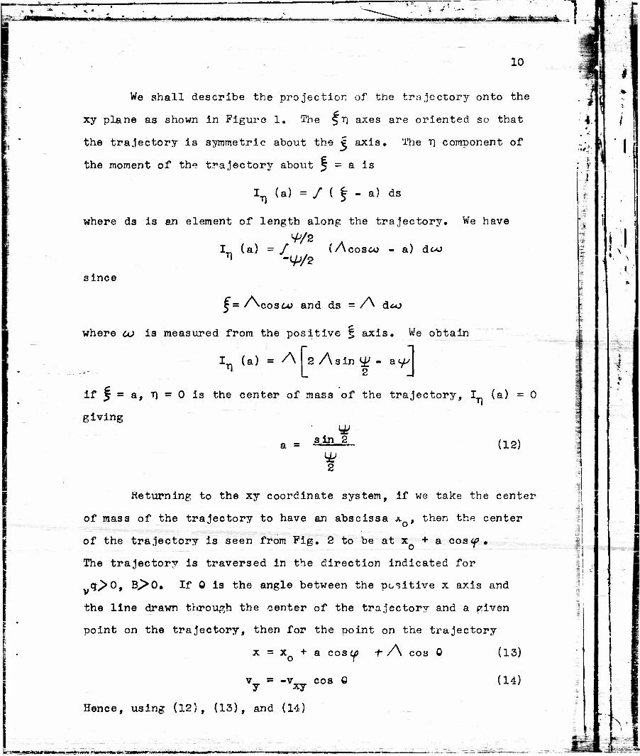
We shall describe the projection of the trajectory onto the

xy plane as shown in Figure 1. The $T] axes are oriented so that

the trajectory is symmetric about the £ axis. The f) component of

the moment of the trajectory about 5 = a is

!„ («) = / ( f - a) ds

where ds is an element of length along the trajectory. We have

1^ (a) = / (Acosco - a) doo

since

c = Acoso; and ds = /> d^o

where to Is measured from the positive 5 axis. We obtain

1^ (a) = A 2'Aaintf- a</J

if 5 = a, T] = 0 is the center of mass of the trajectory, I (a) = 0

giving

a = _ sin 2

2

(12)

Returning to the xy coordinate system, if we take the center

of mass of the trajectory to have an abscissa A , then the center

of the trajectory is seen from Pig. 2 to be at x + a cos<p.

The trajectory is traversed in the direction indicated for

q^O, B,>0# If 0 is the angle between the positive x axis and

the line drawn through the center of the trajectory and a given

point on the trajectory, then for the point on the trajectory

x = x„ + a cos V t /\ co:

vw - -v- cos 6 7 xy

(13)

(14)

Hence, using (12), (13), and (14)

i:' 1

1

J! ,1

BWBW *M<*'WnMi._J""'.iiu-u •** tl L

•-• .-*w*in.. iiiw<y*!!y*jff

XV = 7

4 ^ , A sin ~ A 2 -v__(x_cos© +/\ n^ cos^> cose + /\cos © )

XV 0 2

11

(15)

We shall now average over the tra lectors b^ operating with

We obtain

(xV© = vxy x_coscpSinf + /\

2

sin2 ^ 2 2 cos a;

* (16)

- A f. sino, \ g ^X y^ C TJ

where the subscript © indicates that the average over © has been

carried out.

We now average over all possible orientations of the projec-

tion of the trajectory by operating with

We obtain

. <»TV ^S. iin2^t - l

*'

(17)

Now, if the mean free path of a particle is X, then the probability

of its traveling a distance s between collisions is exp £-s/x] (l/X).

But*-p= s//\ . Thus, the average over s gives

I -.— "••in •! immnim J '_ • •' r »w >»uiwiii_in—ie'iiilpy-i-i .j.

:i"Uv-*^ • ~J**:jh--:

-J—.. X.

TT *.:,.*U——

<*Ve?s Av

•VOD

xi exn(-s/X) «9- -1 d(f)

12:

i

,A *Z

J33

2A ( . / 2A dtl exp ;i - -*-* u * 2 sin u rr~ -J-

(18)

which may be integrated to giv<

I

I

(XV ) = ^La \ 2A

Using (11) we obtain

Arctan 7^ 2X In 1 <*».

-1> (19)

V ..x v B = m (vv*y), |sA c v v'y v~* 2

Thus

r 2 . v"

Arctan X~M» (><£>] •']

tt m( v )* + *- xv B v x' c v v y v

m < ( v ) v ) v x

+ I <vV)2

(20L

X ±. A Arctan ^-gln I 1 + y^ j J -1

However, we exDect the velocity to be statistically iso-

tropic over the xy plane. Thus

•« i

•

( v )2 = - ( v )2 Vx' 2 vv xy' (21)

and we obtain

.m( v )2 + ~ .x v B v v x c v v y = f (x/A) vm(vvx) (22)

1 whe r e

H •-•-'-—avna»'>a*w=^«teaB—' " ' '••*•'-*mnmi tin**-itfmammmRii&HNlGHIBBHR t*wwWiimi.|»jW|w»wwes;.|.|..i i'"-'

1 **Z ' •• ' r TT"

f(X/A) = ^

We note that

f(x)

Arc tan 7^: -r^r- in 6 X2

"7?

, 1 2 1 4 , _6 / x 1 ~ g x + -^ x +0 (x)

f(x)~ *-£ 2 + ln(l + x*)

We rewrite (7), (8), and (9) as

x, + °~6 '*'

ftz: .v•1 = f(vA) z. v»(/x)'

13

(23)

(24)

* I

^IvVyv7 = f(VA)

_d_ dt-

vm(vVyr

vmvvzvz =. V 2

(25)

(26)

I

(24), (25), and (26) are not sufficient to determine the form

of /o(x, y, z). They represent a restriction on the system of

particles under consideration, though they by no means determine

a unique state of the system. The-^ give no information concerning

the form of the spatial distribution of the particles. Hence in

order to use (24), (25), and (26) we must supply a form of distri-

bution over space. (24), (25), and (26) will then tell us how

the scale of the distribution varies with time. With three

equations it is obvious that the form of the distribution may

be characterized bv three riarameters, one parameter describing

the scale of the distribution in each of the three cirections.

At first thought it seems a serious drawback that our

equations will not supply us with the form of the soatial dis-

tribution as well as its variation with time. However, it must

U *\ 1

SB?S^?i:-rft« kk

i

14

be -emembered that the main difficult'"- in oroblems in transport

theory when the solution is attempted f r ~m the Boltzmann equation

is the tremendous mathematical complexitv of the oroblen. The

complexity is brought about by our having to determine simultan-

eously the form of the spatial distribution as well as the

variation with time. Hence we must cut down on the amount of

information that we seek to obtain from our calculations,

supplying the deficit by some informed estimates. The weakness

of our method is, then, the source of its main advantage. In

most cases the form of the soatial distribution is not as impor-

tant to us as the variation in time and is usually known fairly

well anyway. The theory of stochastic processes, for instance,

tells us that in most cases the snatial distribution will be

gaussian for sufficiently large values of time. The end result

is that in practice we may assume a form for the snatial distri-

bution characterized by three units of scale, one in each

direction, and determine the variation with time of the three

units of scale and ultimately of the spatial distribution .

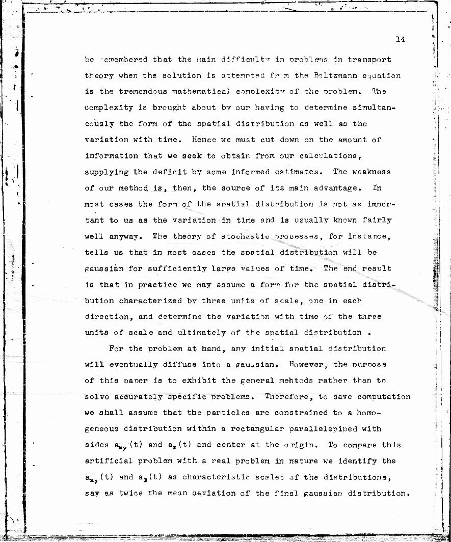
For the problem at hand, any initial snatial distribution

will eventually diffuse into a gaussian. However, the nuroose

of this paner is to exhibit the general mehtods rather than to

solve accurately specific problems. Therefore, to save computation

we shall assume that the particles are constrained to a homo-

geneous distribution within a rectangular parallelepii)ed with

sides a„ -(t) and a,(t) and center at the origin. To compare this

artificial problem with a real problem in nature we identify the

a^ (t) and aa(t) as characteristic scales of the distributions,

say as twice the mean deviation of the final gaustsian distribution.

ii

i

\

i

i

; I

V -*-.——•—-—

**ggfifl6CB£S3SEI - i fif •jaBMWg5^BB8@E|£g*,g

i»PiayP"W.U HM»rir - -rfc.1 • tefc

•••• -"Pi.:- :._jL-i. TT"

> it II

A

3

1F>

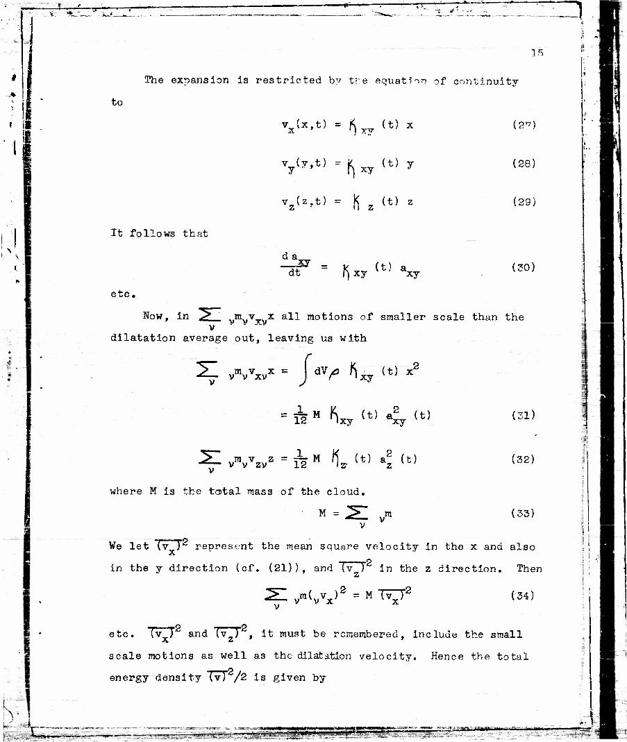
The expansion is restricted by the equation of continuitv

to

vx(x>t} = *)*•* (t> x

v (y,t) - K w (t) y y ' • ' " F| xy

vz(z,t) = |< (t) z

(2*)

(28)

(29)

It follows that

da. _xy _

dt fjxy (t) *Scy (30)

6 vC •

Now, in ^ vmvv-]rvx a11 ^otio"3 °f smaller scale than the v - "V

dilatation average out, leaving us with

vmvvxvx = J dV fix, U) *'

• i M ^xy <*> 4r (t)

vvzvz = l?M 1*(t> 4 (t)

where M is the to>tal mass of the cloud.

M = .m

(31)

(32)

(33)

We let {v ) represent the mean square velocity in the x and also x

in the y direction (cf. (21)), and (v ) in the z direction. Then z

vm(vvx)2=MTv7T2 (34)

e to. (v^T and Tv^T , it must be remembered, include the small

scale motions as well as the dilatation velocity. Hence the total 2 energy density (v) /2 is given by

i i : i

• ^Wv;-;'r; "*—-- •:••> -.• .--v'^, .*••?:•

If

16

\^ = *(\^r) +?^p" —2

(35)

Conservation of energ-f implies that v is independent- of t.

Using (31) and (34), we may now write (24) nnd (25) as

_d_ dt Wt] <7 U). = 12 f(x/A) TTT

(32) gives (26) as

dt uw Using (30) we obtain

d " 't) a? (t) = 12 TFT2

ft [v(t) ft axy(t)] = 12 f(VA) nrr2

D It I az^ ft S(t il - 12 "^7

(36)

(37)

Let us consider several special solutions of (36) and (37).

If B is sufficiently small or f> sufficiently large, then X<< /\

and f (X/A)'"~» 1. Hence the diffusion is unhindered by B and we

have an isotropic adiabatic expansion. We take

In place of (36) and (37) we obtain the single equation

which may be written

= 4 v

•^+ (ft) - A —2 = 4 v (38)

1

•1!

m^SS^

I I

• •

I1

^^M.MaON

JL. ft —•

17

S •' ,,'<

It should be noted that sufficient expansion will eventually

increase "K to where it is no longer less than /\ .

If we consider the other extreme of a stronr field and/or a

low density, "kP&/\, and f (X//\)'"s-0. The cloud exoands only

in the z direction. The enerry of the expansion is

2

iMi.<« ?]•-*&) (59)

The energy of all motions of smaller scale than the parallelepiped

is, then,

(40) 1 „ ^2 . 4 fel) 2 " V 24 \ dt /

(We note the division of the motion into two components defending

uuon the scale relative to the region considered. More will he

said on this in 2.2L) Assuming this energy to be distributed

isotropically over the three dimensions, we have T as just the

energy in the dilatation velocity nlus one thir

in the small scale motion,

mergy

zz 24 dt 3 dt/

M 6

2 V 24 dt /

^+l ("dtV

(41)

Thus, (37/ becomes

a -2o u az

2 d,2

/ \2

(42)

Ncv let us put no restrictions on X but constrain the particles

so that there is no expansion in the z direction. This can be

done by considering the region confined between two material

planes i rpendicular to the z axis.

II I !• V I III III »ll lllll ——»—~ ----- .-K. -.--..-._ •••-: .••.•:':'.- •_;-«?!

iTWifriifw "i*

i

1 I i

f

* * •i •" •—r

18

Analogous to (39), it can be shown that the energy of the

expansion in the x and y directions is each given by (M/24)(da /dt) .

Thus, the motions oT smaller scale than the region have an energy

2 v 12

/da V w (43)

And, assuming isotropy, T and T are lust equal to the energy ' <• •' » xx yy

of the dilatation olus one third, of the small scale energy given

in (43).

xx Xyy 24 \ dt / 3 2 V 12 \ dt /

-»!*•>(>£ (44)

(36) becomes

'xy T^1 * t1 " * f (VA)] (TP) = "(VA> ~2

(38), (42), and (45) are all of the same general form

(45)

6x \dxj (46)

where a and P are constants if we neglect the variation of X with

the expansion. To integrate (46) we let p = dy/dx and write

.2

dx £_Z = 3E _ dp.

2 dx p dy (47)

We obtain

U*/ a _ 1 -prr (48)

where C is the c istant of integration.

Let us assume that when t = 0 there is no expansion and

y = y • (48) becomes

^•^or^-^'^Bgiaaij-'-'. •-rw-^-J'wg ;..... ~ =i^"S*^«a3I3S&is5 i5ssKii] BeK"-i ^;»*-s.. ~* •!*'-•• -:'

MMB9

19

dx a ff) 2a

(49)

Thus, W3 obtain the solution hy quadrature,

x =

a -,

(50) 2a 2a

7 - v " o

For (38) we have a = 1 and B = 4 v2. (49) and (50) give the

rate of expansion of each face of the parallelepiped as

2 J 1/2 lAa(t) -J~^~ \l - 2 dt

and the length of each side as

2

a(o) attT

-p .2

(51)

a(t) - a^o) = 4 72 t

For large values of t we note that the velocity of expansion

(52)

2 dt a(t) v2 (53)

in agreement with the usual result for expansion into a vacuum.

For (42), a = 1/3, 8 = 4 ~v2. (49) and (50) give

2/3 ) 1/2

2 dt lda* -/T* 1 -

az(o) aTtT (54)

t - 2/3/. N _a ' (t) - a 2 V 3 v2

For large values of t, the rate of expansion is

1 11 '2 r * 2/3(o) J '• La2/5(t) + 2a^3(o)j (55)

i da x Z 2 dt ^/3v2 (56)

Finally, for (46)

a = 1 - i f(V,A)

S ^ 4fU/\) "v2

Sstl

I 1 i

: v

- i

"51 91

Hi • -4

to

"'*f

1

,: afes=r;_3?l! aaas^;-fni|fnff,r "".'' **""•''*

ii£afca«te: •"•gMMtB^BIKte

20

We obtain the diffusion rate as

n da 2 dt

fU/A) v2

1 - i f (X/A)

1/S

1 - aKY(0)

L *y

2(l-f (X/A)/3J 1/2 (57)

For large values of t,

2 dt f(X/A) yg

1 - i f (X/A )

1/2

(58)

We note that if X<</\, f(X/A)—' 1 and

-, da 2 dt •V 3 v ^2

(59)

(50) results in an integral which must be evaluated numerically

except for special values of f (X/A) •

If one wishes to consider further complications such as a

uniform distribution of neutral particles which inhibit the dif-

fusion of the charged particles, one introduces an additional

force into ^> P x^ due to collisions of the charged with the

neutral particles.

2.12 As an example of a diffusion problem consider a snace

filled with a homogeneous distribution of neutral particles. At

time t we murk every particle within the rectangle with sides o

a « a , and a and center at the origin. We ask how these marked x* y* z particles will be spread out at some subsequent time t. As has

been pointed out, the tensor virial equations do not determine

the form of the spatial distribution, but, upon assuming some

spatial distribution, indicate how it will vary with time. It is

convenient to express this idea by stating that we use the

tensor virial equations to determine the dynamical conditions for

#

y

ii V •

I

i§ I

.

m

-

B •

jfc

|

•£

w.;,:i!iiiiiTi-in 'jmg&mmmmtBMmsaStffijg }

mm^mmmmme

21

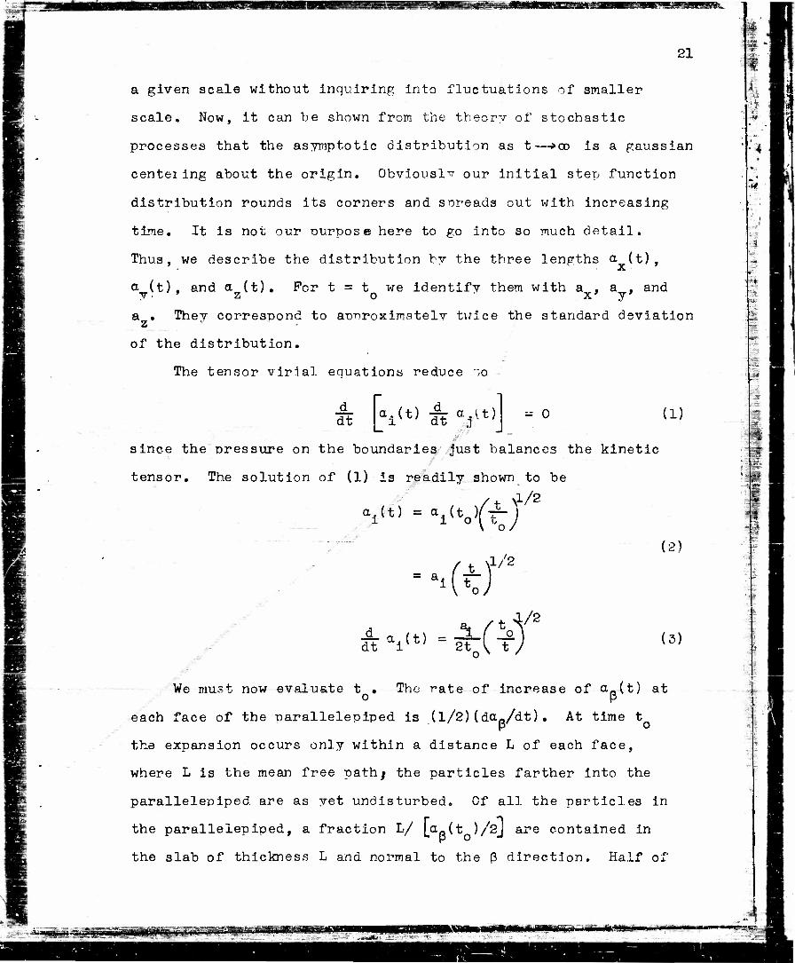
a given scale without inquiring into fluctuations of smaller

scale. Now, it can be shown from the theory of stochastic

processes that the asymptotic distribution as t—*OD is a gaussian

centeiing about the origin. Obviously our initial step function

distribution rounds its corners and spreads out with increasing

time. It is not our ourpose here to go into so much detail.

Thus, we describe the distribution by the three lengths a (t),

a (t), and a (t). For t = t we identify them with a , a , and T • 2 o ' x y' a . They correspond to approximately twice the standard deviation

2

of the distribution.

The tensor virial equations reduce :o

dt [al(t) A a. U) ^ 0 (1)

since the pressure on the boundaries just balances the kinetic

tensor. The solution of (1) is readily shown to be

vL/2 tti(t) = ai(to(t)

/ *. \l/2 (2)

= a. 1 t.

-S- a (t) = dt iKZ) 2t -i r*Jf t / (3)

i -..

m • v

II -I

We must now evaluate t • The rate of increase of &-(t} at o P

each face of the parallelepiped is (1/2)(da«/dt). At time t

the expansion occurs only within a distance L of each face,

where L is the mean free path; the particles farther into the

parallelepiped are as yet undisturbed. Cf all the particles in

the parallelepiped, a fraction L/ Lao^ )/2j are contained in

the slab of thickness L and normal to the p direction. Half of

•

^i^tefijpfraiWBBi MW m**nmt «» am, • —

22 1

these particles are moving outward across the lace with a velocity

y(y*T • Therefore, the fraction L/afi(t ) of the oarticles have p o

a velocity i/iv*)* outward across a face normal to the 6 direction,

We write that the rate of change of the characteristic length

aR(t)/2 is

_d_ dt

!fiiii ^v vw (4)

of time t . Putting t = t in (3) and comparing with (4), we

obtain 2

* - \— 0 4L-/T^f2

Thus, from (2) and (3) we obtain

o1(t) = 2 [h ifWp t]1^

(5)

ft ai(t) = W3"

• '/e

(6)

(7)

One advantage of this method is obviously the doing away

with the infinite diffusion rate obtained at t = t if the oroblem o

were formulated in the conventional manner in terms of V^ . The

thermal diffusion equation is altered to give a finite rate of

propagation of thermal disturbances.

2.2 Let us use (1.1.12) to derive the equations of motion of

a finite region of fluid. We consider a finite region moving

with the fluid. We denote the center of mass of the region by

the cartesian coordinates x . We shall locate points within the

region relative to the center of mass of the region by the

coordinates § , so that the coordinates of the vth particle

become

•*P— rjuf ipa fimm*' '' — 86"i«ii~i"rfr"iTr>ii •;

. X~ = X" V V

The velocity of the vth particle is

v at

which we shall find convenient to write as

Cle arly

y - v1 • /

rf - £ V*X . 0

23

(1)

(2)

(3)

(4)

We refer to the u as the local and v as the translocal

velocity field of the region. Thus, the local field is the portion

of the velocity composed of fluctuations of smaller scale than

the region. Or, in other words, the local field is the portion

which does average out^ the translocal field is the oortion of

the velocity field which does not average out over the region.

Prom (1.1.5) - (1.1.7) and (4) it follows that

rlj' = MxV + m t1 u^ V V V

i:

t

ii

-.,

i - J» -

r

T~ y1 FJ = x1 V v V V

!TiJ = Mv1^ + > m u1 u^

(1.1.12); becomes after sone rearranging of terms

l u1 uJ + 2" ft F1

v v -fr— v * v

_d_ dt m |J u1 v v- V

(5)

\

I i

MjjiMwwii nwnwir m> i isaeigi l[ iy ;«Tm l> t*

1 .-"<•

24

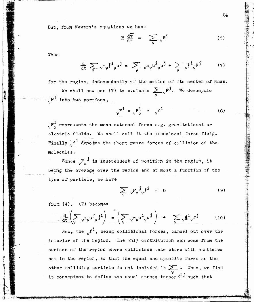
But, from Newton's equations we have

K^1 = 1 A*- (6)

Thus

dt vmv f1 J = - vmv u u^ + V^ V

(v)

for the region, independently of the motion of its center of mass

We shall now use (7) to evaluate F^. We decompose

F into two portions,

pi _ pi + > V o

(8)

F represents the mean external force e.g. gravitational or

electric fields. We shall call it the translocal force field.

Finally f denotes the short range forces of collision of the

molecules.

Since F ^ is independent of nosition in the region, it

being the average over the region and at most a function of the

type of particle, we have

F J I1 V O V

= 0 (9)

from (4). (7) becomes

_d_ dt £ uU* vmv- V \v

vVV3 j 4i rl V"* V" (10)

Now, the f , being collisional forces, cancel out over the

interior of the region. The only contribution can come from the

surface of the region where collisions take place with particles

net in the region, so that the equal and opposite force on the

other colliding particle is not included in Thus, we find i *

it convenient to define the usual stress tensor o~^ such that

:J -.-~^J,i><Wi<it yrmc*x.'jjcjrji'MMFT"'"•- >«ih>- ;»-;gf?MlHHHft* mmm mmmm mmmm •••

1^ <

I •I \

i

i •

-

ii

25

ic 6 dS Is the force in the idirection across an element of area

dS normal to the a direction. 6 ' represents the force exerted

by the matter on the nositive side of dS on the matter on the 5

negative side. This is the customary definition in elasticity

and electromagnetic theory. We shall replace ^> by intepration v

over the elements of volume dV.

The introduction of a stress tensor and the associated

processes and parameters such as integration, differentiation,

pressure, viscosity, etc. requires a limited form of continuity

in our hitherto unrestricted system* Our notion of infinitesimal

becomes that of the physical infinitesimal, viz. that the smallest

elements of volume dV that we consider must be sufficiently

large as to contain a large number of particles. If n represents

the number of particles in dV, then the fluctuation of n is of

the order of -V~rT . We must require that

VrT < < n

in order that our averaging process over dV have a smoothing

effect. To be treated as an infinitesimal, dV, of course, must

be of smaller scale than the phenomena in which we are interested.

The alternative to these restrictions on dV is to consider an

ensemble of systems so that the average may be carried out over

the given dV in each member system rather than .lust a single

system.

We rewrite (10) as

dt (jdV^jV) = jdV^uV) + jdskS

16J1 (11)

Gauss' theorem gives

V

i i

••

S5

i

s

mmm i i mwrnmss^mmm •B pyuiii;*"' " mrw»»mur.

26

.d dt -((dV^V^) = jdV^uV1) + (dV^ktf1^*) (12)

-jdV^uV) +(dVdU H-^1^

jk

ai- ds)

-3(5^ /3| reDresents the force in the i direction oer unit

volume. The translocal portion of -3<3^ /3f , given to acceler-

ating the entire region, cannot contribute to )dV| 3d^ /df .

This j.s readily shown if we note that the translocal portion of

-3d3k/3*ik is defined as

3c5^k \ _ _dvJ

H* /x

(14)

Then

Wf{^\ -f H1

a

= o

by (.4).

The remaining portion of 3c5^' /3<f is local to the region

and is responsible for changing the shaoe of the region. Since • *

6 ** is the only stress field present, it follows that if the 1k / k local component of do> /3§ vanishes, then the region is in

equilibrium. We have dJ *ydt = 0 or,

and (13) becomes

0 = ) dV^uV + ^ dVd1J (15)

T -A I

-;!

-*&M&&m&2 ftM^S^ftfe***^^ i^ssa^ff^j"^saK^:,«^r^f?^--w^ WSJ***? ~*r*i J -err*-.

27

which has the solution a

61* = -/OU u yO •n ** (16)

:*

= -2T ij (17)

I i •

Prom (8) and (l1?) we obtain

F 5- + C dsv<5ik

> o J k

r P i . r 7 v ° )

dV-4=-(/0u1uk)

(6) becomes

M^1 = dt 7^ - jdV^(^!

t^iJ1

(is)

Consider now (x> u"""uJ). If there is no shearing of the

region, we expect no correlation over the region between u. and

u'1. Hence (ouV) is zero if i ^ j. The diagonal terms are

nonzero and give the pressure. If, however, there is an overall

shearing of the region, we see that -there w.ill be a correlation

between u and u^ for i / j. Let the shearing be renr-esented by

i 3

45 o v or "We see, then, that 2T •* represents the integral . . the region of • the Reynolds or kinetic .stresses , wV"? .-.n mav be represented by pressure, 2Taa , and shearing stress -2TaP. <5>ij , as in (1.1.12), represent the integral over the region of all other stress fields, e.g. pravity, electric fields, etc. If we denote by IP-J the sum of the Reynolds and all other stress fields, then (1.1.12) may be written

dt Jij = Y.

If ^11 vanishes, so also aoes dJ^/dt, at greater length in 3.1.

This will be discussed

\

«. — •'«5as*33SSE? zKj&&&skm*-: —••**•>-

28 m

3v /dx** If the average scale in the P direction of the local

i R R velocity field u is denoted by Lr , then with a velocity u we

expect to find associated a velocity -L^3v /3x^ in the a direction.

Hence, we write

(19) ox

X

ox

for a ^ p. We define

and write more generally

a S

M- = Lo U L )

—a (/OU up) = -<^6

aacS P3 8v aa ay *;P a *IP 3x a

(20)

(21)

•

- -

Thus, we rewrite (18) as

3xa dV -| PP^ ^

3 3xP 9xP

(22)

which is the equation of motion for a finite region of fluid.

.<£

-

2.21 Let us consider some snecial cases of the eq-uati^ns of

motion of a finite volume of fluid expressed in (2.2.22). If

we consider an incompressible flow, then

3 - ° ax1 *

and the last term in (2.2.22) becomes

3 /act av ^c^y = )OTS h^ (i)

If there are no compressibility effects, then to a fair degree of

A 3S@mgI^IIIIH'J.HI II || IN'i i" iflKIBI IHjes^SaS^W^SS*^^

M

29

ctci approximation the variation of " ji in -"he direction of the flow

may be neglected. Hence, we are able to rewrite (2.2.22) as

H dv _ dt > F a + \dV ~tf — v o j -s—a v J 3x

aa

J (3 3XP PPU Sv^ (2)

.aa aa

We note that

dv = - P

where p is the pressure in the a direction. Tbas, if there is

an approach to isotropy in the local motions, we write

P = - §<5h -x (3)

HI*

= rl/OU u.; O ' 1

and the second term in (2) becomes

dv~4^aa = - dv^a 3x 3x

(4)

(5)

It is of interest to compare (4) with Batchelor's value computed

by Fourier transform methods from the theory of isotropic turbulence,

Again, if there is an approach to isotropy in the local

motions, we define

u = (-v uxu.) (6)

so that we may write

L = (VL1^)

a 1 - U = -7= U

.a

(7)

(8)

(9)

"HsH3R»»ii«!£***««* t^,^-XK3^\i^<»'>**ZBZi^*rii\Utt&fa5txij&;»-S

.. ..-.*.**«**«

,;yta!5;iaagg^l.3; jnywacua* -* •

T-p. .

Assuming no correlation betwesn u and L , we obtain

aa = "S" /O u« ^OUi

30

(10)

:•

is i -

and rewrite (2) for the case of isotropic local motions as

J ax1 I ax1

(11)

*§f - 5Z P a - (dv %„ (12)

If we let the size of the region approach zero, we obtain

the usual Navier - Stokes equations for an incompressible fluid,

,—a dv Fa 1 8^ . 8 dt 70 , a „„i

J. -a i v

8xx y (13)

dx 3x'

where P is the force oer unit mass and v is [1//O . p and ^

are due only to the thermal motions, i.e. motions local to a

scale of zero.

_

2.22 It should be noted that " u- and p or I 6 |.f and therefore

p and u- are monotonical y increasing- functions of the size of

the region considered, v' and its space and time derivatives, on

the other hand, are monotonically decreasing functions of the

size of the region.

It is of interest to note how with the tensor virial

equation the velocity field v naturally resolves itself into

the translocal and local velocity fields v and u . We note that

only the statistical characteristics of the local field aonear in

the field equations of the translocal field, (2.2.22) Thus, we

are not surprised to see the emergence of Prandtl's mixing length

concept in computing (ou u") for i ^ j. Altogether, then, it

a

i 1 •

k

••'.^•^'»itm&^^^^Wt''t,,^>^^s^!^F;i^'ilS!S^;'' :-yir itmmrwxsi ggemsaww*-

& j;ii i, 11 aw iwffw i -wit—in m • mrngy»wr»" ~»^

31

would seem that the statistical representation of Prandtl's

mixing length theory and the more extensive treatment carried 7 Q 9

out in Heisenberg's field equation ' and elsewhere follow quite

naturally from the tensor viriai equations of motion.

2.3 The tensor viriai equations are particularly suited to

investigation of the d^manics of finite r egions of matter. The

following examples are typical of those encountered in astro-

physics in the treatment of gas clouds, star clusters, etc. and

in diffusion problems. In the treatment of the dynamics of ras

clouds the tensor viriai equations are convenient becaus,e even

with very artificial constraints the question of whether a term

is to be included as a Potential enerp:-^ or as a kinetic energy

is easily decided.

2.31 Consider the radial oscillation of a gas cloud in its own

gravitational field. The tensor viriai equations d~s not give us

the radial distribution matter. To prevent the mathematics from

becoming too complex we introduce the constraint that the density

be homogeneous within the sphere of radius r (t) about the

origin and zero outside. Thus, the radial velocity at any ooint

within the cloud is

o (1)

The motion of the system is thus describable by the single

parameter r . Hence, we use the scalar viriai equation (1.2.3) o

It is readilv shown that

V = - 5GM2

5r 12)

I

awNHWt jUii jMiHnii^wgBMIlJI—k* n

I = 4r M r 2 lO o

32

(3)

where M is the mass of the sohere. The contribution of the radial

oscillations to T is

T, = gr M[ -^S) (4)

Let us assume that the motions of smaller scale than r follow o polytrope law so that

where

—•• = TTTffVT " 3 o I r_

oo o o

A corresponds to the usual y~ written when only thermal motions

are considered. For instance, if there is no dissipation,

A = 5/? for turbulence and for the thermal motions in monatomic

gases. If more than one type of local motion is oresent, we write

0 ,'T \3 (A - 1) 2T„ =M > TTT2 ( -?& ) a (5) a o l r^ a \ o

•

"

(1,2.3) becomes

A2

d ro JL2

7-T-T2 „ 3(A -1) c . \v ) r ^ a _ 5 ^r— a o oo 3 ^— 3A -2

_ _£M_ dt a rQ a ro2

a o a ^Aa" nVro

(6)

after cancelling out a factor of 3M/lOs CJpon integration vje

obtain the energy equation

•

where c is the total energy per unit mas3. We obtain r (t) by

quadrature as

n-ii•~»;»i:;H3;: rfflWfrlHW" ' t >W9 mi.11.

M^MHapaiaawseaBg -; - ?** - •as; = ? i ii a—i

33

t - t .A dr,

\ rio £_ 10 ^-TvTT^ /r00 . r j oo

,3(A„ - 1) 2GM

(8) 1/2

2.32 One finds in his applications of the tensor virial equations

that he usually uses rectangular parallelepipedal or ellipsoidal

regions, In the case that the repion is an isolated one,the

parallelepiped becomes inconvenient because of the extreme

complexity of the force field expressions from which the potential

12 tensor is computed. The expressions for the contribution to

the potential tensor of the mutual inverse square interactions of

the particles composing a homogeneous ellipsoid are recorded here.

If external forces are present there will, of course, be an

additional contribution to the potential tensor. The expressions

derived.in this section have been applied elsewhere to problems 2

in galactic dynamics.

Consider ^articles of matter distributed uniformlv throughout

the interior of an ellipsoid with semi-axes a. Without loss of

generality we orient our axes so that

(1) 1> 2> 3 a ^ a — a

12 It can be shown for gravitational interaction that

.aa £— = _JL GM2(aa)2 N° (2)

i •

i!

-

where M is the mass of the ellipsoid and

2

N2 =

N-"- = tu1)4 - iTif6 -\ [v - E(uj,k)

[(a1)2 - (a3) 2 . ( E(o.k)

k*(l -k*) (1- kc)

3TV cnv dnv

(3)

\( (4)

-

) tuiri llflWjgMMW •JIMIffl rMmmflre%s«a^^ - omm mm»-

•

N3 = [(a1)2 - (a5)2]3^ I snv dhv w . x / i

cnv , .2 ) l - k

34

(5)

where

/ /a3 r • 3 2

.into = snv = / 1 -/Ar- ) , cnv = j" » ^"v = ^T (6) V \& I a a

(ax)2 - (a3)2 (7)

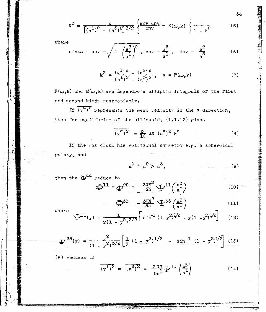
F(uj,k) and E(co,k) are Legendre's elliptic integrals of the first

and second kinds respectively.

If (v ) represents the mean velocity in the a direction,

then for equilibrium of the elliosoid, (1.1.12) gives

(va)2 =^ GM (aa)2 Na (8)

If the f£3 cloud has rotational symmetry e.g. a soheroidal

galaxy, and

(9) 1 2^3 a = a > a ,

aa then the <£> reduce to

..11 .22 3GM' 5a ' *"($)

where

^**s33 _ 3GM2 v3>33 /a3>\

(10)

(11)

^w - ; hrsTsC3*""1 ^-y2)^ - yd -/>V2] ^2> 2(1 - j)6/iiL-

1

x ' V *

> i

:

I ^55(y) = (l-y2)3/2Ly(1-y2) 2vl/S , -1 M 2x1/2 s in 11 - y ; • \-L<-'/

(8) reduces to

t ^2 (v ) / 2x2 (v ) 3GM,Tyll

5a m (14)

HUM. —ME S"«.«rs«S^ 'rawrmpui- • Www. -

3*2 3GM '\a = 5aJ *33 {$) (15)

o. 2 It would be well to rcemohasize the fact that the (v )

are the mean square values of the local velocity field and need

not Be random in the usual sense. We nnlv require that the

average <J£ v over the region vanish. Thus the rotational velocity

of the region as well as smaller scale turbulence and therrral

velocities are oart of the local velocitv field and make uo

(v ) . For instance, if we consider a sohericdal ralax?/- in whii

the velocities local to the rotation are isotronic, it fellows

that the rotation velocity vw is

<02 = S^v1)2- (v3)2]

from (14) and (15).

Stress Tensor Formulation i

3.1 Having discussed the tensor virial equations in terms of

the kinetic and potential tensors, let us now state the relations

in terms of stress tensors. This formulation is particularly

13 useful when dealing with problems in magnetohydro dynamics. We

shall assume oonderamotive forces repr-esentabl e bv the general

stress tensor Z.J Then (1.1.12) mav be written*1*

|S ^dV/ovV = jdV^ovV + [ dSkxJ(5ik + jdVx* ^ Zik (l)

in cartesian coordinates. It should be noted that we cannot

'See formulation from Newton's equations in Aooendix A.

-_?~. mmm LpWH.^jJUP gia«j|gpWf^aHWiWI BjaggafC Slii»X-»l"?tl J

?6

!i

*

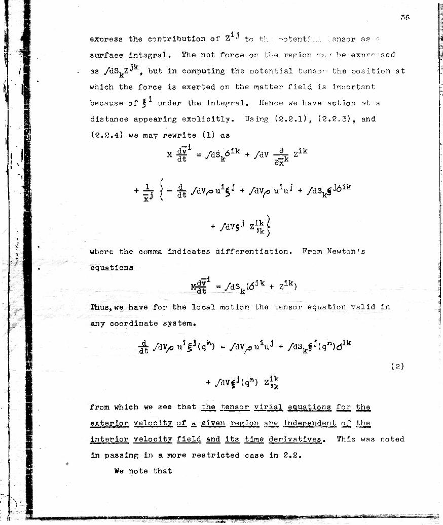
exoress the contribution of Z •' to th : ^otent:... Censor as >?

surface integral. The net force or the rerion ia-.' be ext>re?sed

as y'dS.Z*' , but in computing the potential tenso-" the oosition at

which the force is exerted on the matter field is important

because of J under the integral. Hence we have action at a

distance appearing exolicitly. Using (2.2.1), (2,2.3), and

(2.2.4) we may rewrite (l) as

,-i M * = M>lk * /dV 4v Z1] dt 3x*

+ rj [ - It /dVuV + /dV> uiuj + /dSi^ J6ik

+ /dV|J z1*

where the comma indicates differentiation. Prom Newton's

equations

,ri :3k , „Ik, Mli =/dSk^aK + zlK)

Thus, we have for the local motion the tensor equation valid in

any coordinate system.

,icjr„n i.J lhnn\^^ •g£ /dV* Ui|J(q'1) = /dV^u^u"1 + /dSkf J(q")d

(2)

+ /dV|^(qn) Z ik >k

from which we see that the tensor viriai equations for the

exterior velocity of a given region are independent of the

Interior velocity field and its time derivatives. This was noted

in passing in a more restricted case in 2,2.

We note that

\ ,

H xm mm—pwp • •ntpw —ahMHWWBW w»«*»g ~irnmrrMP"1 -r"' -•-•«• I

i

I

37

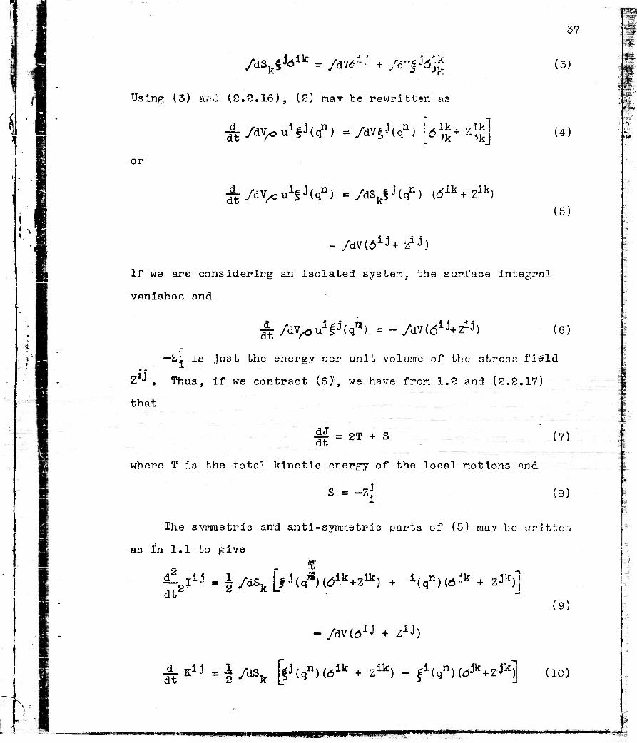
/dS fkik = /dVrf1"' + /d"jJtf" (3)

Using (3) a/.^ (2.2.16), (2) mav be rewritten as

-^/dV^ouVU11) =/dV|-^(qn) xik, 7ik 4>k+Zik (4)

or

^r/dVuV(qn) =/dSkf^(qn) (<5ik+Zik)

- /dv(6i;J+ Z1^)

(5)

If we are considering an isolated system, the surface integral

vanishes and

^ /dV^u1!J(q*) = - /dV^+Z^) (6)

—2.. is ju3t the energy oer unit volume of the stress field

ZlJ . Thus, if we contract (6)', we have from 1.2 and (2.2.17)

that

im

m • M

. S3.

•

• t i

-,

4f = 2T + S at

where T is the total kinetic energy of the local motions and

S = -Z?

(7)

(8)

- . rs

The symmetric and anti-symmetric parts of (5) may be written

as in 1.1 to give if

,2

dt' ,IiJ = § /dSk \tH<j*)Ufr+Z*) + ^q")^* + Z^)J

(9)

- /dV(<51J + Z1^)

JL K^= 1 /dSk [^(qn)(6ik H- Zlk) - f1(qn)(dJk + Z^ (10)

Kin n,lMi«HWBpgg*M«rg3gawP»ii i "» ••' ""» • ' ' "•••' „ j

36

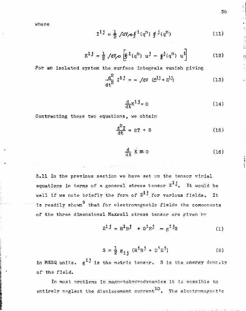
whs re

i/_n. I1J =-|/dV/cf1(qn) ^(qn) (11)

K1J = \ ftf/o (f ^q") U^ - |'(qn) U1 (12)

For an isolated system the surface integrals vanish giving

2 4 i^' = - /dv (6ij' + z^) dtr

(13)

Contracting these two equations, we obtain

dt = 2T + S

(14)

(15)

£K-° (16)

3,11 In the previous section we have set up the tensor virial

equations in terms of a general stress tensor Z J. It would be

well if we note briefly the form of Z vfor various fields. It 9

is readily shown that for electromagnetic fields the components

of the three dimensional Maxwell stress tensor are piven bv

Z1^ = JrV + DiEJ - glj's (1)

,„i_1 rvl.^1, (n B° + D E') (2)

in MKSQ units. gXJ is the matric tensor. S is the energy density

of the field.

M

In most problems in ma/rn^tohydro dynamics it is possible to 10 entirely neglect the displacement current" The electromagnetsc

-4.-;- • .».' ' '-W- •j^ir—rr-lil

39

field becomes, then, a magnetic field and is a "v.:-e r.tres? field

with no associated inertia to be induced in our equations. We

drop the terms involving the electric fie]d so that

Z1^ = H^" - gi;JS (3)

S=|giJH-H M (4)

Further simplification may be carried out since the permeability

of the conducting fluid usually aoproximates very closely to

empty space and is in any case isotropic and homogeneous.

In the case of a gravitational field v:e have the field

intensit^r <JJ ~ given in terms of a scalar \L according to

\±J± = -y+A (5)

so that

M *iJ V.i.l = 4TlG. r/° (6)

"IT* i --•

r.

'I •: I

/

k :

V *

*.i = - 4itG /°

The force ner unit volume is

P1 =/o^i

(7)

- •

C=0

Thus, in order- that

p1 = Zik

the s tress tensor is defined as

zii i- L^ W- g 4irG

,k

i^L „ij„]

(9)

(10)

-•.-i*Mi.-,S4je-i'.<v;p-=

* I""* '.'•ffi.C^ ***-*i»--i

<mg» wi nwiff' mmi- i .-.i"."u u' -r ii , " ^."* ,ii/-. BS ^Vi"

40

1

where

W = | vj, * v^. ,1

(11)

In order to derive (8) from (9) and (10) we note from (4) that

the curl of '-X'" is zero.

The total energy of the field is

S = -Z*

W 4-rtG

8iG^ ^i (12) .i

Conclusion

m

4.1 It was Dointed out in 2.22 that the ideas basic to Drand.tl's

and Heisenberg's formulations of turbulence theory arise as a

natural consequence of the tensor virial formulation of the

equations of p^otion. Let us summarize the more important of these

principles.

The effect of multiplying by J before summing over the

particles in the region is to cancel out the effects of force and

velocity fluctuations of larger scale than the reg?':n considered.

The result is a separation of all effects into the loc-l and trans-

local components. It was then shown in 3.1 that the local tensor

virial equations are indenendent of the translocsl field. (2.2.18)

shows that the translocsl field denencs on;v on the statistical

orooerties of the local field. We found in 2.2 that the statistical

:i

!

-'"•" tV-:

atFvWt&je&tttzx^'-w&awemmmmBsaEE.* -rj(fc»tf¥a

41

pronerties of the local field relevant to a calculation of the

translocal field nay be constructed in a natural way from a

characteristic length and velocity of the local field, both of

which depend upon the scale of the region used.

i

!- N i a n

IN L £* t n*5****8* • * ,«7»' -'-• f^ftT—.+ • 'a*^g8iSWggP «w»H^=>yilrtrw:e

h i s

mmi *i.. »'•• w. ••--*!*» V '^jl /-• ijKMJp '*#' '.'•*

»3ny '-'s-

3-1

I, It i a m f

VI

42

Appendix A

Ln 1.1 the terror vi.'ial equations were cievelooed in

co.rtesian coordinates. Let us nov* ver brieflv out] ine their

develoonent :n a general coordinate system. Let the coordinates

of the vth particle •Z • Let the -ocsition of the vth narticle

relative to the or^'p . "he ^^rssBnu^ by the vector & ( q ). We

note that

The Lagrengian equation., of ration are

(1)

rtk -i a i v^ \\'° ) V (2)

and are readi!,-; sp^n to be covariant and of rank one because L

is a scalar, dt is an invariant, and th Q. satisfy (1.1.2) in

which 5 W is a scalar. M' n tinl^inp- by §,^( q ), (2) may he

written as

l\. , L °„ q ° ,3 a q

(3) o q v^ a q" v^

(1.1.5) — (1.1.8) are redefined as

-1 VlJ (vq } TY± V

Ik 3L PT^ = > £^ a'

<2>j, = <Tl\qk>

V

3L .i 3 q-

(4)

(5)

(6)

^•-.•Mik^j&x'jIM^JrJ**.: .— Wl«i» imwwii^JitWWMt

••

I .'- * i

—.-#•»• »ya>-•--,* -j -vBbap •mtiiia^r-'*sg»«»fe«rSi *•'-«*-•& • •••*• ,*^->•--••*

!i

I

I

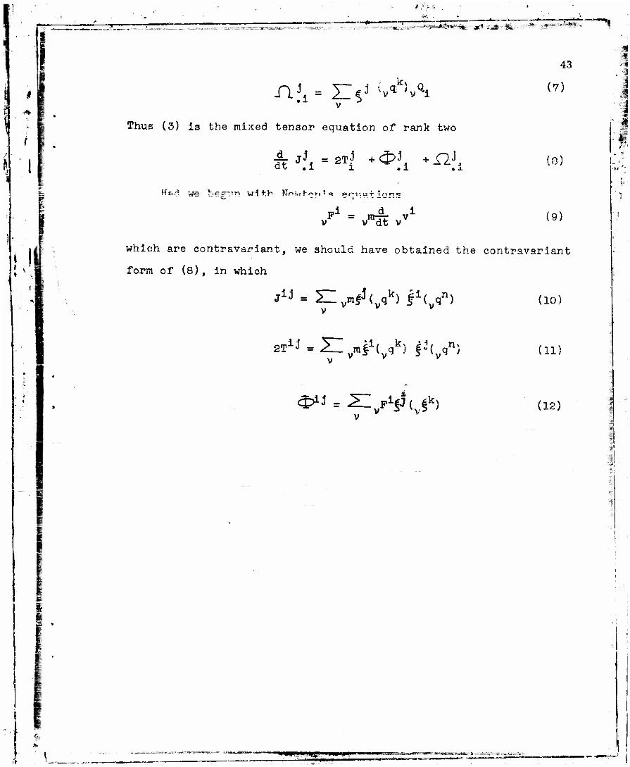
Thus (3) is the mixed tensor equation of rank two

43

(7)

dt .1

^&v We hcFtlTI with NpUit'nri'a »rr»af lyHS

v v dt v (9)

which are contravariant, we should have obtained the contravariant

form of (8), in which

J1* = Hvm^(vqk) f\<f)

2Tij = Zl mfH qk) f-\ qn) v

V ^ V5 '

(10)

(11)

(12)

I

•WgWJt.. I'M i»". HI in* null i IIII i*—•— --1' ••"i •••

c

i :\ .

f

V ,

44

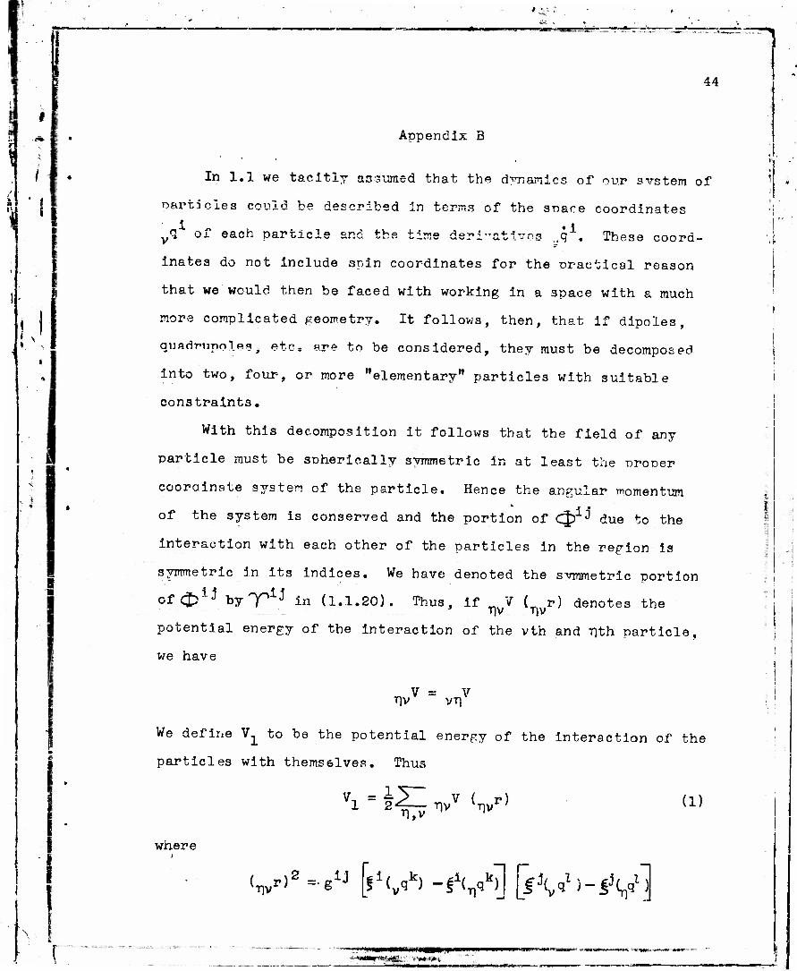
Appendix B

In 1.1 we tacitly assumed that the dynamics of our svstem of

particles could be described in terms of the soace coordinates

yq of each particle and the time derivatives ,,q . These coord-

inates do not include spin coordinates for the practical reason

that we would then be faced with working in a space with a much

more complicated geometry. It follows, then, that if dipoles,

quadripole*, etc, are to be considered, they must be decomposed

into two, four, or more "elementary" particles with suitable

constraints.

With this decomposition it follows that the field of any

particle must be spherically symmetric in at least the orooer

coorainate system of the particle. Hence the angular momentum

of the system is conserved and the portion of Cj) J due to the

interaction with each other of the particles in the region is

symmetric in its indices. We have denoted the symmetric portion

of c£>1;5 byTiJ in (1.1.20). Thus, if V ( r) denotes the

potential energy of the interaction of the vth and T}th particle,

we have

t *

V -• V T}V VT)

We define Vx to be the potential energy of the interaction of the

particles with themselves. Thus

*i = ill .vv (wp) Tl.V

(1)

wnere

«W'>"-61J i\ft -fV>] [iV'-lVi

W—Mm I Ml |

45

V. is the local portion of V.

If we define L^ as the local portion of L, i.e. due to the

interaction of the particles in the region with each other, then

from (1.1.7) we have in cartesian coordinates that

-r-j - ~ 8 x v

3

!

E

!

r1* = -r- y avn

3 xJ

= ~s- x1 -d— vx ST r T1,V

--x: TJV L_

V( r) 7]V T}V

1 a^

a x-

i -1, -3

T1VJ W^m,** Jagj-jgV

S r V

%,>v'

3nvV'^'((v^-n^'v^-^3' 3„ r 71V

( r)

iy - y) (vxJ • y)

T),V '

3-,v(^.r) (^1-T1xi)( xJ- xj)

vr)v (2)

We see that 7^^ = p as required. Let us diagonalize T1!

by referring it to itr principal axes. We have, then, only the

three terms I , Repeated Greek indices do not imoly summation

convention. / is the contribution to the potentialtensor of

the forces and displacements in the a direction.

If the V( r) are homogeneous of degree n, then

T^:=-|X .w»<•r) n,v

a a x — x v B_

Tlvr (3)

I ;

I <

,

•i*v..;'•'.. -..,--» —_TS^„.as sahwaJ— Ml—wwn

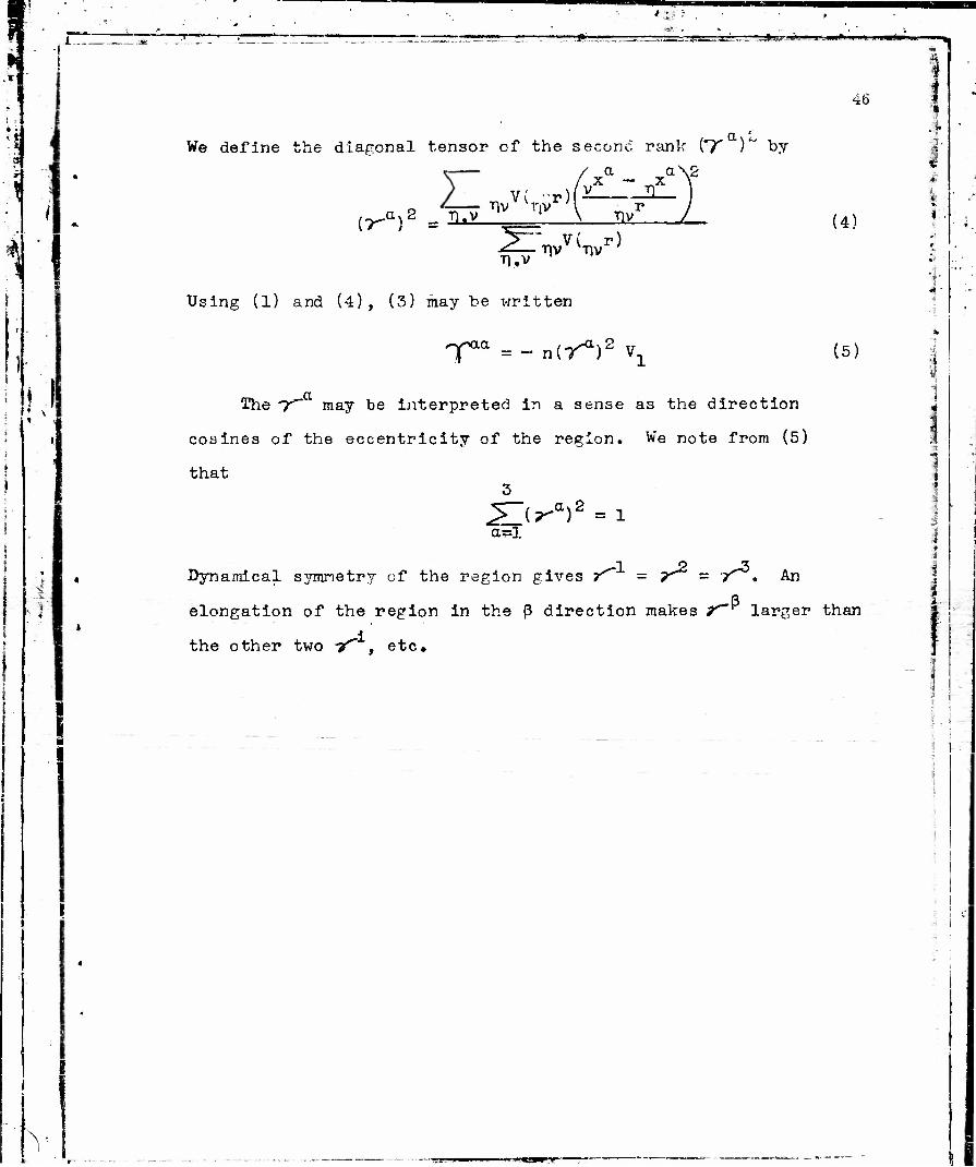
46

i 8

We define the diagonal tensor of the second rank ("7" )*" by a a\2

V( r)P-

•^-- T1V TlV •n,v

•nv XTIV

Using (1) and (4), (3) may be written

(4)

1 1

i

-f• =- nO^)2 V1 (5)

The 7"" may be interpreted in a sense as the direction

cosines of the eccentricity of the region. We note from (5)

that 3

~S^1 (^a)2 = 1

Dynamical symmetry cf the region gives Y^" - 7^ - ir . An

elongation of the region in the P direction makes

the other two y , etc.

larger than

1 I i

\ •.

I

•A

\

l\

i -

•Wfc- VVJMnWMIMMi ̂

47

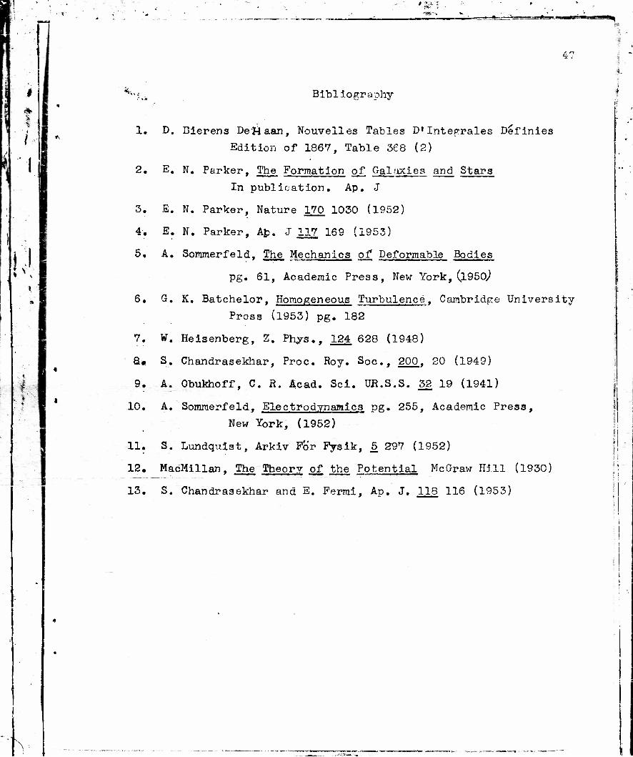
*k, Bibliography

1. D. Bierens De&aan, Nouvelles Tables D1 Inteprales Definies

Edition of 1867, Table 368 (2)

2. E. N. Parker, The Formation of Galaxies and Stars

In publication. Ap. J

3. E. N. Parker, Nature 170 1030 (1952)

4. E. N. Parker, Ap. -J 117 169 (1953)

5. A. Sommerfeld, The Mechanics of Deformable Bodies

pg. 61, Academic Press, New York, (i960,)

6. G. K. Batchelor, Homogeneous Turbulence. Cambridge University

Pross (1953) pg. 182

7. W. Heisenberg, Z. Phys., 124.628 (1948)

8« S. Chandrasekhar, Proc. Roy. Soc, 200_, 20 (1949)

9. A. Obukhoff, C. R. Acad. Sci. UR.S.S. 32 19 (1941)

10. A. Sommerfeld, Electrodynamics pg. 255, Academic Press,

New York, (1952)

11. S. Lundquist, Arkiv For Fysik, 5 297 (1952)

12. MacMillan, The Theory of the Potential McGraw Hill (1930)

13. S. Chandrasekhar and E. Fermi, Ap. J. 118 116 (1953)

3.

-rr-

I

I ! i •

Figure 1

Figure 2

I 1

I