physicsreferencemanual€¦ · 9.7.5 algorithm for polarized radiation . . . . . . . . . . . . 165...

Physics Reference Manual

Version: geant4 10.2 (4 December 2015)

Contents

I Introduction 1

1 Introduction 21.1 Scope of This Manual . . . . . . . . . . . . . . . . . . . . . . . 21.2 Definition of Terms . . . . . . . . . . . . . . . . . . . . . . . . 2

2 Monte Carlo Methods 4

3 Particle Transport 63.1 True Step Length . . . . . . . . . . . . . . . . . . . . . . . . . 8

3.1.1 The Interaction Length or Mean Free Path . . . . . . . 83.1.2 Determination of the Interaction Point . . . . . . . . . 93.1.3 Step Limitations . . . . . . . . . . . . . . . . . . . . . 93.1.4 Updating the Particle Time . . . . . . . . . . . . . . . 10

3.2 Transportation . . . . . . . . . . . . . . . . . . . . . . . . . . 11

II Particle Decay 13

4 Decay 144.1 Mean Free Path for Decay in Flight . . . . . . . . . . . . . . . 144.2 Branching Ratios and Decay Channels . . . . . . . . . . . . . 14

4.2.1 G4PhaseSpaceDecayChannel . . . . . . . . . . . . . . . 154.2.2 G4DalitzDecayChannel . . . . . . . . . . . . . . . . . . 154.2.3 Muon Decay . . . . . . . . . . . . . . . . . . . . . . . . 164.2.4 Leptonic Tau Decay . . . . . . . . . . . . . . . . . . . 174.2.5 Kaon Decay . . . . . . . . . . . . . . . . . . . . . . . . 17

III Electromagnetic Interactions 19

5 Gamma Incident 205.1 Introduction . . . . . . . . . . . . . . . . . . . . . . . . . . . . 21

-10

5.1.1 General Interfaces . . . . . . . . . . . . . . . . . . . . . 215.2 Photoelectric Effect . . . . . . . . . . . . . . . . . . . . . . . . 23

5.2.1 Cross Section . . . . . . . . . . . . . . . . . . . . . . . 235.2.2 Final State . . . . . . . . . . . . . . . . . . . . . . . . 235.2.3 Relaxation . . . . . . . . . . . . . . . . . . . . . . . . . 24

5.3 Compton scattering . . . . . . . . . . . . . . . . . . . . . . . . 265.3.1 Cross Section . . . . . . . . . . . . . . . . . . . . . . . 265.3.2 Sampling the Final State . . . . . . . . . . . . . . . . . 275.3.3 Atomic shell effects . . . . . . . . . . . . . . . . . . . . 28

5.4 Gamma Conversion into an Electron - Positron Pair . . . . . . 305.4.1 Cross Section . . . . . . . . . . . . . . . . . . . . . . . 305.4.2 Final State . . . . . . . . . . . . . . . . . . . . . . . . 345.4.3 Ultra-Relativistic Model . . . . . . . . . . . . . . . . . 35

5.5 Gamma Conversion into a Muon - Anti-mu Pair . . . . . . . . 375.5.1 Cross Section and Energy Sharing . . . . . . . . . . . . 375.5.2 Parameterization of the Total Cross Section . . . . . . 405.5.3 Multi-differential Cross Section and Angular Variables 425.5.4 Procedure for the Generation of µ+µ− Pairs . . . . . . 44

6 Elastic scattering 526.1 Multiple Scattering . . . . . . . . . . . . . . . . . . . . . . . . 53

6.1.1 Introduction . . . . . . . . . . . . . . . . . . . . . . . . 536.1.2 Definition of Terms . . . . . . . . . . . . . . . . . . . . 546.1.3 Path Length Correction . . . . . . . . . . . . . . . . . 566.1.4 Angular Distribution . . . . . . . . . . . . . . . . . . . 586.1.5 Determination of the Model Parameters . . . . . . . . 586.1.6 Step Limitation Algorithm . . . . . . . . . . . . . . . . 606.1.7 Boundary Crossing Algorithm . . . . . . . . . . . . . . 626.1.8 Implementation Details . . . . . . . . . . . . . . . . . . 63

6.2 Discrete Processes for Charged Particles . . . . . . . . . . . . 666.3 Single Scattering . . . . . . . . . . . . . . . . . . . . . . . . . 68

6.3.1 Coulomb Scattering . . . . . . . . . . . . . . . . . . . . 686.3.2 Implementation Details . . . . . . . . . . . . . . . . . . 69

6.4 Ion Scattering . . . . . . . . . . . . . . . . . . . . . . . . . . . 716.4.1 Method . . . . . . . . . . . . . . . . . . . . . . . . . . 716.4.2 Implementation Details . . . . . . . . . . . . . . . . . . 75

6.5 Single Scattering, Screened Coulomb Potential and NIEL . . . 776.5.1 Nucleus–Nucleus Interactions . . . . . . . . . . . . . . 776.5.2 Nuclear Stopping Power . . . . . . . . . . . . . . . . . 796.5.3 Non-Ionizing Energy Loss due to Coulomb Scattering . 826.5.4 G4IonCoulombScatteringModel . . . . . . . . . . . . . 83

6.5.5 The Method . . . . . . . . . . . . . . . . . . . . . . . . 836.5.6 Implementation Details . . . . . . . . . . . . . . . . . . 84

6.6 Electron Screened Single Scattering and NIEL . . . . . . . . . 866.6.1 Scattering Cross Section of Electrons on Nuclei . . . . 866.6.2 Nuclear Stopping Power of Electrons . . . . . . . . . . 956.6.3 Non-Ionizing Energy-Loss of Electrons . . . . . . . . . 96

6.7 G4eSingleScatteringModel . . . . . . . . . . . . . . . . . . . . 976.7.1 The method . . . . . . . . . . . . . . . . . . . . . . . . 986.7.2 Implementation Details . . . . . . . . . . . . . . . . . . 100

7 Energy loss of Charged Particles 1027.1 Mean Energy Loss . . . . . . . . . . . . . . . . . . . . . . . . 103

7.1.1 Method . . . . . . . . . . . . . . . . . . . . . . . . . . 1037.1.2 General Interfaces . . . . . . . . . . . . . . . . . . . . . 1047.1.3 Step-size Limit . . . . . . . . . . . . . . . . . . . . . . 1047.1.4 Run Time Energy Loss Computation . . . . . . . . . . 1067.1.5 Energy Loss by Heavy Charged Particles . . . . . . . . 107

7.2 Energy Loss Fluctuations . . . . . . . . . . . . . . . . . . . . . 1097.2.1 Fluctuations in Thick Absorbers . . . . . . . . . . . . . 1097.2.2 Fluctuations in Thin Absorbers . . . . . . . . . . . . . 1107.2.3 Width Correction Algorithm . . . . . . . . . . . . . . . 1127.2.4 Sampling of Energy Loss . . . . . . . . . . . . . . . . . 112

7.3 Correcting the Cross Section for Energy Variation . . . . . . 1147.4 Conversion from Cut in Range to Energy Threshold . . . . . . 1167.5 Photoabsorption ionization model . . . . . . . . . . . . . . . . 119

7.5.1 Cross Section for Ionizing Collisions . . . . . . . . . . . 1197.5.2 Energy Loss Simulation . . . . . . . . . . . . . . . . . 1217.5.3 Photoabsorption Cross Section at Low Energies . . . . 1227.5.4 Status of this document . . . . . . . . . . . . . . . . . 123

8 Electron and Positron Incident 1248.1 Ionization . . . . . . . . . . . . . . . . . . . . . . . . . . . . . 125

8.1.1 Method . . . . . . . . . . . . . . . . . . . . . . . . . . 1258.1.2 Continuous Energy Loss . . . . . . . . . . . . . . . . . 1258.1.3 Total Cross Section per Atom and Mean Free Path . . 1278.1.4 Simulation of Delta-ray Production . . . . . . . . . . . 128

8.2 Bremsstrahlung . . . . . . . . . . . . . . . . . . . . . . . . . . 1308.2.1 Seltzer-Berger bremsstrahlung model . . . . . . . . . . 1308.2.2 Bremsstrahlung of high-energy electrons . . . . . . . . 133

8.3 Positron - Electron Annihilation . . . . . . . . . . . . . . . . . 1388.3.1 Introduction . . . . . . . . . . . . . . . . . . . . . . . . 138

8.3.2 Cross Section . . . . . . . . . . . . . . . . . . . . . . . 1388.3.3 Sampling the final state . . . . . . . . . . . . . . . . . 1388.3.4 Sampling the Gamma Energy . . . . . . . . . . . . . . 139

8.4 Positron Annihilation into µ+µ− Pair in Media . . . . . . . . . 1418.4.1 Total Cross Section . . . . . . . . . . . . . . . . . . . . 1418.4.2 Sampling of Energies and Angles . . . . . . . . . . . . 141

8.5 Positron Annihilation into Hadrons . . . . . . . . . . . . . . . 1458.5.1 Introduction . . . . . . . . . . . . . . . . . . . . . . . . 1458.5.2 Cross Section . . . . . . . . . . . . . . . . . . . . . . . 1458.5.3 Sampling the final state . . . . . . . . . . . . . . . . . 145

9 Low Energy Livermore 1479.1 Introduction . . . . . . . . . . . . . . . . . . . . . . . . . . . . 148

9.1.1 Physics . . . . . . . . . . . . . . . . . . . . . . . . . . . 1489.1.2 Data Sources . . . . . . . . . . . . . . . . . . . . . . . 1489.1.3 Distribution of the Data Sets . . . . . . . . . . . . . . 1499.1.4 Calculation of Total Cross Sections . . . . . . . . . . . 150

9.2 Compton Scattering . . . . . . . . . . . . . . . . . . . . . . . 1519.2.1 Total Cross Section . . . . . . . . . . . . . . . . . . . . 1519.2.2 Sampling of the Final State . . . . . . . . . . . . . . . 151

9.3 Compton Scattering by Linearly Polarized Gamma Rays . . . 1539.3.1 The Cross Section . . . . . . . . . . . . . . . . . . . . . 1539.3.2 Angular Distribution . . . . . . . . . . . . . . . . . . . 1539.3.3 Polarization Vector . . . . . . . . . . . . . . . . . . . . 1539.3.4 Unpolarized Photons . . . . . . . . . . . . . . . . . . . 154

9.4 Rayleigh Scattering . . . . . . . . . . . . . . . . . . . . . . . . 1559.4.1 Total Cross Section . . . . . . . . . . . . . . . . . . . . 1559.4.2 Sampling of the Final State . . . . . . . . . . . . . . . 155

9.5 Gamma Conversion . . . . . . . . . . . . . . . . . . . . . . . . 1569.5.1 Total cross-section . . . . . . . . . . . . . . . . . . . . 1569.5.2 Sampling of the final state . . . . . . . . . . . . . . . . 156

9.6 Pair production by Linearly Polarized Gamma Rays . . . . . . 1589.6.1 Relativistic cross section for linearly polarized gamma

ray . . . . . . . . . . . . . . . . . . . . . . . . . . . . . 1589.6.2 Spatial azimuthal distribution . . . . . . . . . . . . . . 1599.6.3 Unpolarized Photons . . . . . . . . . . . . . . . . . . . 160

9.7 Triple Gamma Conversion . . . . . . . . . . . . . . . . . . . . 1629.7.1 Method . . . . . . . . . . . . . . . . . . . . . . . . . . 1629.7.2 Azimuthal Distribution for Electron Recoil . . . . . . . 1629.7.3 Monte Carlo Simulation of the Asymptotic Expression 1629.7.4 Algorithm for Non Polarized Radiation . . . . . . . . . 163

9.7.5 Algorithm for Polarized Radiation . . . . . . . . . . . . 1659.7.6 Sampling of Energy . . . . . . . . . . . . . . . . . . . . 167

9.8 Photoelectric effect . . . . . . . . . . . . . . . . . . . . . . . . 1699.8.1 Cross sections . . . . . . . . . . . . . . . . . . . . . . . 1699.8.2 Sampling of the final state . . . . . . . . . . . . . . . . 1699.8.3 Angular distribution of the emitted photoelectron . . . 169

9.9 Electron ionisation . . . . . . . . . . . . . . . . . . . . . . . . 1729.10 Bremsstrahlung . . . . . . . . . . . . . . . . . . . . . . . . . . 174

9.10.1 Bremsstrahlung angular distributions . . . . . . . . . . 175

10 Low Energy Penelope 18110.1 Penelope physics . . . . . . . . . . . . . . . . . . . . . . . . . 182

10.1.1 Introduction . . . . . . . . . . . . . . . . . . . . . . . . 18210.1.2 Compton scattering . . . . . . . . . . . . . . . . . . . . 18210.1.3 Rayleigh scattering . . . . . . . . . . . . . . . . . . . . 18410.1.4 Gamma conversion . . . . . . . . . . . . . . . . . . . . 18510.1.5 Photoelectric effect . . . . . . . . . . . . . . . . . . . . 18710.1.6 Bremsstrahlung . . . . . . . . . . . . . . . . . . . . . . 18810.1.7 Ionisation . . . . . . . . . . . . . . . . . . . . . . . . . 19010.1.8 Positron Annihilation . . . . . . . . . . . . . . . . . . . 196

11 Monash University low energy photon processes 19911.1 Monash Low Energy Models . . . . . . . . . . . . . . . . . . . 200

11.1.1 Introduction . . . . . . . . . . . . . . . . . . . . . . . . 20011.1.2 Physics and Simulation . . . . . . . . . . . . . . . . . . 200

12 Charged Hadron Incident 20312.1 Ionization . . . . . . . . . . . . . . . . . . . . . . . . . . . . . 204

12.1.1 Method . . . . . . . . . . . . . . . . . . . . . . . . . . 20412.1.2 Continuous Energy Loss . . . . . . . . . . . . . . . . . 20412.1.3 Nuclear Stopping . . . . . . . . . . . . . . . . . . . . . 20912.1.4 Total Cross Section per Atom . . . . . . . . . . . . . . 20912.1.5 Simulating Delta-ray Production . . . . . . . . . . . . 21012.1.6 Ion Effective Charge . . . . . . . . . . . . . . . . . . . 211

12.2 Low energy extentions . . . . . . . . . . . . . . . . . . . . . . 21312.2.1 Energy losses of slow negative particles . . . . . . . . . 21312.2.2 Energy losses of hadrons in compounds . . . . . . . . . 21312.2.3 Fluctuations of energy losses of hadrons . . . . . . . . 21412.2.4 ICRU 73-based energy loss model . . . . . . . . . . . . 216

13 Muon Incident 21813.1 Ionization . . . . . . . . . . . . . . . . . . . . . . . . . . . . . 21913.2 Bremsstrahlung . . . . . . . . . . . . . . . . . . . . . . . . . . 221

13.2.1 Differential Cross Section . . . . . . . . . . . . . . . . . 22113.2.2 Continuous Energy Loss . . . . . . . . . . . . . . . . . 22213.2.3 Total Cross Section . . . . . . . . . . . . . . . . . . . . 22213.2.4 Sampling . . . . . . . . . . . . . . . . . . . . . . . . . 223

13.3 Positron - Electron Pair Production by Muons . . . . . . . . . 22513.3.1 Differential Cross Section . . . . . . . . . . . . . . . . . 22513.3.2 Total Cross Section and Restricted Energy Loss . . . . 22813.3.3 Sampling of Positron - Electron Pair Production . . . . 229

13.4 Muon Photonuclear Interaction . . . . . . . . . . . . . . . . . 23113.4.1 Differential Cross Section . . . . . . . . . . . . . . . . . 23113.4.2 Sampling . . . . . . . . . . . . . . . . . . . . . . . . . 232

14 Atomic Relaxation 23514.1 Atomic relaxation . . . . . . . . . . . . . . . . . . . . . . . . . 236

14.1.1 Fluorescence . . . . . . . . . . . . . . . . . . . . . . . . 23614.1.2 Auger process . . . . . . . . . . . . . . . . . . . . . . . 23714.1.3 PIXE . . . . . . . . . . . . . . . . . . . . . . . . . . . 237

15 Geant4-DNA 23915.1 Geant4-DNA processes and models . . . . . . . . . . . . . . . 240

16 Microelectronics 24116.1 The MicroElec extension for microelectronics applications . . . 242

17 Polarized Electron/Positron/Gamma Incident 24417.1 Introduction . . . . . . . . . . . . . . . . . . . . . . . . . . . . 245

17.1.1 Stokes vector . . . . . . . . . . . . . . . . . . . . . . . 24517.1.2 Transfer matrix . . . . . . . . . . . . . . . . . . . . . . 24717.1.3 Coordinate transformations . . . . . . . . . . . . . . . 24817.1.4 Polarized beam and material . . . . . . . . . . . . . . . 249

17.2 Ionization . . . . . . . . . . . . . . . . . . . . . . . . . . . . . 25217.2.1 Method . . . . . . . . . . . . . . . . . . . . . . . . . . 25217.2.2 Total cross section and mean free path . . . . . . . . . 25217.2.3 Sampling the final state . . . . . . . . . . . . . . . . . 254

17.3 Positron - Electron Annihilation . . . . . . . . . . . . . . . . . 25917.3.1 Method . . . . . . . . . . . . . . . . . . . . . . . . . . 25917.3.2 Total cross section and mean free path . . . . . . . . . 25917.3.3 Sampling the final state . . . . . . . . . . . . . . . . . 261

17.3.4 Annihilation at Rest . . . . . . . . . . . . . . . . . . . 26317.4 Polarized Compton scattering . . . . . . . . . . . . . . . . . . 265

17.4.1 Method . . . . . . . . . . . . . . . . . . . . . . . . . . 26517.4.2 Total cross section and mean free path . . . . . . . . . 26517.4.3 Sampling the final state . . . . . . . . . . . . . . . . . 266

17.5 Polarized Bremsstrahlung for electron and positron . . . . . . 27017.5.1 Method . . . . . . . . . . . . . . . . . . . . . . . . . . 27017.5.2 Polarization in gamma conversion and bremsstrahlung 27017.5.3 Polarization transfer to the photon . . . . . . . . . . . 27117.5.4 Polarization transfer to the lepton . . . . . . . . . . . . 272

17.6 Polarized Gamma conversion into an electron–positron pair . . 27517.6.1 Method . . . . . . . . . . . . . . . . . . . . . . . . . . 27517.6.2 Polarization transfer . . . . . . . . . . . . . . . . . . . 275

17.7 Polarized Photoelectric Effect . . . . . . . . . . . . . . . . . . 27717.7.1 Method . . . . . . . . . . . . . . . . . . . . . . . . . . 27717.7.2 Polarization transfer . . . . . . . . . . . . . . . . . . . 277

18 X-Ray Production 28018.1 Transition radiation . . . . . . . . . . . . . . . . . . . . . . . . 281

18.1.1 Relationship of Transition Rad to Cherenkov Rad . . . 28118.1.2 Calculating the X-ray Transition Radiation Yield . . . 28218.1.3 Simulating X-ray Transition Radiation Production . . . 284

18.2 Scintillation . . . . . . . . . . . . . . . . . . . . . . . . . . . . 28818.3 Cerenkov Effect . . . . . . . . . . . . . . . . . . . . . . . . . . 28918.4 Synchrotron Radiation . . . . . . . . . . . . . . . . . . . . . . 291

18.4.1 Photon spectrum . . . . . . . . . . . . . . . . . . . . . 29118.4.2 Validity . . . . . . . . . . . . . . . . . . . . . . . . . . 29218.4.3 Direct inversion/generation of photon energy spectrum 29318.4.4 Properties of the Power Spectra . . . . . . . . . . . . . 296

19 Optical Photons 29919.1 Interactions of optical photons . . . . . . . . . . . . . . . . . . 300

19.1.1 Physics processes for optical photons . . . . . . . . . . 30019.1.2 Photon polarization . . . . . . . . . . . . . . . . . . . . 30119.1.3 Tracking of the photons . . . . . . . . . . . . . . . . . 30219.1.4 Mie Scattering in Henyey-Greensterin Approximation . 305

20 Phonon-Lattice Interactions 30820.1 Introduction . . . . . . . . . . . . . . . . . . . . . . . . . . . . 30920.2 Phonon Propagation . . . . . . . . . . . . . . . . . . . . . . . 30920.3 Lattice Parameters . . . . . . . . . . . . . . . . . . . . . . . . 310

20.4 Scattering and Mode Mixing . . . . . . . . . . . . . . . . . . . 31020.5 Anharmonic Downconversion . . . . . . . . . . . . . . . . . . . 31120.6 References . . . . . . . . . . . . . . . . . . . . . . . . . . . . . 311

21 Precision multi-scale modeling 31321.1 Overview . . . . . . . . . . . . . . . . . . . . . . . . . . . . . . 31421.2 Impact ionisation by hadrons and PIXE . . . . . . . . . . . . 314

22 Shower Parameterizations 32322.1 Gflash Shower Parameterizations . . . . . . . . . . . . . . . . 324

22.1.1 Parameterization Ansatz . . . . . . . . . . . . . . . . . 32422.1.2 Longitudinal Shower Profiles . . . . . . . . . . . . . . 32422.1.3 Radial Shower Profiles . . . . . . . . . . . . . . . . . . 32522.1.4 Gflash Performance . . . . . . . . . . . . . . . . . . . . 326

IV Hadronic Interactions 328

23 Total Reaction Cross Section in Nucleus-nucleus Reactions 32923.1 Sihver Formula . . . . . . . . . . . . . . . . . . . . . . . . . . 32923.2 Kox and Shen Formulae . . . . . . . . . . . . . . . . . . . . . 33023.3 Tripathi formula . . . . . . . . . . . . . . . . . . . . . . . . . 33223.4 Representative Cross Sections . . . . . . . . . . . . . . . . . . 33423.5 Tripathi Formula for ”light” Systems . . . . . . . . . . . . . . 334

24 Coherent elastic scattering 33924.1 Nucleon-Nucleon elastic Scattering . . . . . . . . . . . . . . . 339

25 Hadron-nucleus Elastic Scattering at Medium/High Energy34025.1 Method of Calculation . . . . . . . . . . . . . . . . . . . . . . 340

26 Interactions of Stopping Particles 35626.1 Complementary parameterised and theoretical treatment . . . 356

26.1.1 Pion absorption at rest . . . . . . . . . . . . . . . . . . 357

27 Parton string model. 35927.1 Reaction initial state simulation. . . . . . . . . . . . . . . . . . 359

27.1.1 Allowed projectiles and bombarding energy range . . . 35927.1.2 MC initialization procedure for nucleus. . . . . . . . . 35927.1.3 Random choice of the impact parameter. . . . . . . . . 361

27.2 Sample of collision participants in nuclear collisions. . . . . . . 36127.2.1 MC procedure to define collision participants. . . . . . 361

27.2.2 Separation of hadron diffraction excitation. . . . . . . . 36227.3 Longitudinal string excitation . . . . . . . . . . . . . . . . . . 363

27.3.1 Hadron–nucleon inelastic collision . . . . . . . . . . . . 36327.3.2 The diffractive string excitation . . . . . . . . . . . . . 36327.3.3 The string excitation by parton exchange . . . . . . . . 36327.3.4 Transverse momentum sampling . . . . . . . . . . . . . 36427.3.5 Sampling x-plus and x-minus . . . . . . . . . . . . . . 36427.3.6 The diffractive string excitation . . . . . . . . . . . . . 36427.3.7 The string excitation by parton rearrangement . . . . . 365

27.4 Longitudinal string decay. . . . . . . . . . . . . . . . . . . . . 36627.4.1 Hadron production by string fragmentation. . . . . . . 36627.4.2 The hadron formation time and coordinate. . . . . . . 367

28 Fritiof (FTF) Model 36928.1 Main assumptions of the FTF model . . . . . . . . . . . . . . 37028.2 General properties of hadron–nucleon interactions . . . . . . . 373

28.2.1 π−p – interactions . . . . . . . . . . . . . . . . . . . . . 37328.2.2 π+p – interactions . . . . . . . . . . . . . . . . . . . . . 37528.2.3 pp – interactions . . . . . . . . . . . . . . . . . . . . . 37628.2.4 K+p – and K−p – interactions . . . . . . . . . . . . . . 37728.2.5 pp – interactions . . . . . . . . . . . . . . . . . . . . . 379

28.3 Cross sections of hadron–nucleon processes . . . . . . . . . . . 38128.3.1 Total, elastic and inelastic hadron–nucleon cross sections38128.3.2 Cross sections of quark exchange processes . . . . . . . 38328.3.3 Cross sections of antiproton processes . . . . . . . . . . 38328.3.4 Cross sections of diffractive and non-diffractive processes384

28.4 Simulation of hadron-nucleon interactions . . . . . . . . . . . 38728.4.1 Simulation of meson–nucleon and nucleon–nucleon in-

teractions . . . . . . . . . . . . . . . . . . . . . . . . . 38728.4.2 Simulation of antibaryon–nucleon interactions . . . . . 390

28.5 Flowchart of the FTF model . . . . . . . . . . . . . . . . . . . 39128.6 Simulation of nuclear interactions . . . . . . . . . . . . . . . . 393

28.6.1 Sampling of intra-nuclear collisions . . . . . . . . . . . 39328.6.2 Reggeon cascading . . . . . . . . . . . . . . . . . . . . 39928.6.3 ”Fermi motion” of nuclear nucleons . . . . . . . . . . . 40628.6.4 Excitation energy of nuclear residuals . . . . . . . . . . 409

29 Bertini Intranuclear Cascade Model in Geant4 41329.1 Introduction . . . . . . . . . . . . . . . . . . . . . . . . . . . . 41329.2 The Geant4 Cascade Model . . . . . . . . . . . . . . . . . . . 414

29.2.1 Model Limits . . . . . . . . . . . . . . . . . . . . . . . 414

29.2.2 Intranuclear Cascade Model . . . . . . . . . . . . . . . 41429.2.3 Nuclear Model . . . . . . . . . . . . . . . . . . . . . . 41529.2.4 Pre-equilibrium Model . . . . . . . . . . . . . . . . . . 41729.2.5 Break-up models . . . . . . . . . . . . . . . . . . . . . 41729.2.6 Evaporation Model . . . . . . . . . . . . . . . . . . . . 418

29.3 Interfacing Bertini implementation . . . . . . . . . . . . . . . 418

30 The Geant4 Binary Cascade 42130.1 Modeling overview . . . . . . . . . . . . . . . . . . . . . . . . 421

30.1.1 The transport algorithm . . . . . . . . . . . . . . . . . 42130.1.2 The description of the target nucleus and fermi motion 42230.1.3 Optical and phenomenological potentials . . . . . . . . 42330.1.4 Pauli blocking simulation . . . . . . . . . . . . . . . . . 42430.1.5 The scattering term . . . . . . . . . . . . . . . . . . . 42430.1.6 Total inclusive cross-sections . . . . . . . . . . . . . . 42530.1.7 Channel cross-sections . . . . . . . . . . . . . . . . . . 42530.1.8 Mass dependent resonance width and partial width . . 42630.1.9 Resonance production cross-section in the t-channel . . 42630.1.10Nucleon Nucleon elastic collisions . . . . . . . . . . . . 42730.1.11Generation of transverse momentum . . . . . . . . . . 42730.1.12Decay . . . . . . . . . . . . . . . . . . . . . . . . . . . 42830.1.13The escaping particle and coherent effects . . . . . . . 42830.1.14Light ion reactions . . . . . . . . . . . . . . . . . . . . 42930.1.15Transition to pre-compound modeling . . . . . . . . . . 42930.1.16Calculation of excitation energies and residuals . . . . 430

30.2 Comparison with experiments . . . . . . . . . . . . . . . . . . 430

31 Quantum Molecular Dynamics for Heavy Ions 43931.1 Equations of Motion . . . . . . . . . . . . . . . . . . . . . . . 44031.2 Ion-ion Implementation . . . . . . . . . . . . . . . . . . . . . . 44231.3 Cross Sections . . . . . . . . . . . . . . . . . . . . . . . . . . . 443

32 Abrasion-ablation Model 44532.1 Introduction . . . . . . . . . . . . . . . . . . . . . . . . . . . . 44532.2 Initial nuclear dynamics and impact parameter . . . . . . . . . 44632.3 Abrasion process . . . . . . . . . . . . . . . . . . . . . . . . . 44732.4 Abraded nucleon spectrum . . . . . . . . . . . . . . . . . . . . 44932.5 De-excitation of nuclear pre-fragments by standard G4 . . . . 45032.6 De-excitation of nuclear pre-fragments by nuclear ablation . . 45132.7 Definition of the functions P and F used in the abrasion model 452

33 Electromagnetic Dissociation Model 45633.1 The Model . . . . . . . . . . . . . . . . . . . . . . . . . . . . . 456

34 Precompound model. 46034.1 Reaction initial state. . . . . . . . . . . . . . . . . . . . . . . . 46034.2 Simulation of pre-compound reaction . . . . . . . . . . . . . . 460

34.2.1 Statistical equilibrium condition . . . . . . . . . . . . . 46134.2.2 Level density of excited (n-exciton) states . . . . . . . 46134.2.3 Transition probabilities . . . . . . . . . . . . . . . . . . 46134.2.4 Emission probabilities for nucleons . . . . . . . . . . . 46334.2.5 Emission probabilities for complex fragments . . . . . . 46334.2.6 The total probability . . . . . . . . . . . . . . . . . . . 46434.2.7 Calculation of kinetic energies for emitted particle . . . 46434.2.8 Parameters of residual nucleus. . . . . . . . . . . . . . 464

35 Evaporation Model 46635.1 Introduction . . . . . . . . . . . . . . . . . . . . . . . . . . . . 46635.2 Evaporation model . . . . . . . . . . . . . . . . . . . . . . . . 466

35.2.1 Cross sections for inverse reactions . . . . . . . . . . . 46735.2.2 Coulomb barriers . . . . . . . . . . . . . . . . . . . . . 46735.2.3 Level densities . . . . . . . . . . . . . . . . . . . . . . . 46835.2.4 Maximum energy available for evaporation . . . . . . . 46835.2.5 Total decay width . . . . . . . . . . . . . . . . . . . . . 469

35.3 GEM model . . . . . . . . . . . . . . . . . . . . . . . . . . . . 46935.4 Nuclear fission . . . . . . . . . . . . . . . . . . . . . . . . . . . 471

35.4.1 The fission total probability . . . . . . . . . . . . . . . 47135.4.2 The fission barrier . . . . . . . . . . . . . . . . . . . . 471

35.5 Photon evaporation . . . . . . . . . . . . . . . . . . . . . . . . 47235.5.1 Computation of probability . . . . . . . . . . . . . . . 47235.5.2 Discrete photon evaporation . . . . . . . . . . . . . . . 47235.5.3 Internal conversion electron emission . . . . . . . . . . 473

35.6 Sampling procedure . . . . . . . . . . . . . . . . . . . . . . . . 474

36 Fission model. 47736.1 Reaction initial state. . . . . . . . . . . . . . . . . . . . . . . . 47736.2 Fission process simulation. . . . . . . . . . . . . . . . . . . . . 477

36.2.1 Atomic number distribution of fission products. . . . . 47736.2.2 Charge distribution of fission products. . . . . . . . . . 47936.2.3 Kinetic energy distribution of fission products. . . . . . 47936.2.4 Calculation of the excitation energy of fission products. 48036.2.5 Excited fragment momenta. . . . . . . . . . . . . . . . 480

37 Fermi break-up model. 48237.1 Fermi break-up simulation for light nuclei . . . . . . . . . . . . 482

37.1.1 Allowed channels . . . . . . . . . . . . . . . . . . . . . 48237.1.2 Break-up probability . . . . . . . . . . . . . . . . . . . 48337.1.3 Fragment characteristics . . . . . . . . . . . . . . . . . 48437.1.4 Sampling procedure . . . . . . . . . . . . . . . . . . . . 484

38 Multifragmentation model. 48638.1 Multifragmentation process simulation. . . . . . . . . . . . . . 486

38.1.1 Multifragmentation probability. . . . . . . . . . . . . . 48638.1.2 Direct simulation of low multiplicity disintegration . . 48838.1.3 Fragment multiplicity distribution. . . . . . . . . . . . 48938.1.4 Atomic number distribution of fragments. . . . . . . . 48938.1.5 Charge distribution of fragments. . . . . . . . . . . . . 49038.1.6 Kinetic energy distribution of fragments. . . . . . . . . 49038.1.7 Calculation of the fragment excitation energies. . . . . 490

39 INCL++: the Liege Intranuclear Cascade model 49239.1 Introduction . . . . . . . . . . . . . . . . . . . . . . . . . . . . 492

39.1.1 Suitable application fields . . . . . . . . . . . . . . . . 49339.2 Generalities of the INCL++ cascade . . . . . . . . . . . . . . . 494

39.2.1 Model limits . . . . . . . . . . . . . . . . . . . . . . . . 49439.3 Physics ingredients . . . . . . . . . . . . . . . . . . . . . . . . 495

39.3.1 Emission of composite particles . . . . . . . . . . . . . 49639.3.2 Cascade stopping time . . . . . . . . . . . . . . . . . . 49639.3.3 Conservation laws . . . . . . . . . . . . . . . . . . . . . 49739.3.4 Initialisation of composite projectiles . . . . . . . . . . 49739.3.5 De-excitation phase . . . . . . . . . . . . . . . . . . . . 497

39.4 Physics performance . . . . . . . . . . . . . . . . . . . . . . . 497

40 ABLA V3 evaporation/fission model 50240.1 Level densities . . . . . . . . . . . . . . . . . . . . . . . . . . . 50340.2 Fission . . . . . . . . . . . . . . . . . . . . . . . . . . . . . . . 50340.3 External data file required . . . . . . . . . . . . . . . . . . . . 50440.4 How to use ABLA V3 . . . . . . . . . . . . . . . . . . . . . . 504

41 Low Energy Neutron Interactions 50541.1 Introduction . . . . . . . . . . . . . . . . . . . . . . . . . . . . 50541.2 Physics and Verification . . . . . . . . . . . . . . . . . . . . . 505

41.2.1 Inclusive Cross-sections . . . . . . . . . . . . . . . . . . 50541.2.2 Elastic Scattering . . . . . . . . . . . . . . . . . . . . . 506

41.2.3 Radiative Capture . . . . . . . . . . . . . . . . . . . . 50741.2.4 Fission . . . . . . . . . . . . . . . . . . . . . . . . . . . 50841.2.5 Inelastic Scattering . . . . . . . . . . . . . . . . . . . . 512

41.3 Neutron Data Library (G4NDL) Format . . . . . . . . . . . . 51341.3.1 Cross Section . . . . . . . . . . . . . . . . . . . . . . . 51341.3.2 Final State . . . . . . . . . . . . . . . . . . . . . . . . 51441.3.3 Thermal Scattering Cross Section . . . . . . . . . . . . 51441.3.4 Coherent Final State . . . . . . . . . . . . . . . . . . . 51541.3.5 Incoherent Final State . . . . . . . . . . . . . . . . . . 51641.3.6 Inelastic Final State . . . . . . . . . . . . . . . . . . . 517

41.4 High Precision Models and Low Energy Parameterized Models 51941.5 Summary and Important Remark . . . . . . . . . . . . . . . . 519

42 Low Energy Charged Particle Interactions 52142.1 Introduction . . . . . . . . . . . . . . . . . . . . . . . . . . . . 52142.2 Physics and Verification . . . . . . . . . . . . . . . . . . . . . 521

42.2.1 Inclusive Cross-sections . . . . . . . . . . . . . . . . . . 521

43 Geant4 Low Energy Nuclear Data (LEND) Package 52343.1 Low Energy Nuclear Data . . . . . . . . . . . . . . . . . . . . 523

44 Radioactive Decay 52444.1 The Radioactive Decay Module . . . . . . . . . . . . . . . . . 52444.2 Alpha Decay . . . . . . . . . . . . . . . . . . . . . . . . . . . . 52444.3 Beta Decay . . . . . . . . . . . . . . . . . . . . . . . . . . . . 52544.4 Electron Capture . . . . . . . . . . . . . . . . . . . . . . . . . 52544.5 Recoil Nucleus Correction . . . . . . . . . . . . . . . . . . . . 52644.6 Biasing Methods . . . . . . . . . . . . . . . . . . . . . . . . . 526

V Gamma- and Lepto-Nuclear Interactions 528

45 Introduction 529

46 Cross Sections in Photonuclear/Electronuclear Reactions 53046.1 Approximation of Photonuclear Cross Sections. . . . . . . . . 53046.2 Electronuclear Cross Sections and Reactions . . . . . . . . . . 53346.3 Common Notation for Electronuclear Reactions . . . . . . . . 533

47 Gamma-nuclear Interactions 54147.1 Process and Cross Section . . . . . . . . . . . . . . . . . . . . 54147.2 Final State Generation . . . . . . . . . . . . . . . . . . . . . . 541

48 Electro-nuclear Interactions 54348.1 Process and Cross Section . . . . . . . . . . . . . . . . . . . . 54348.2 Final State Generation . . . . . . . . . . . . . . . . . . . . . . 543

49 Muon-nuclear Interactions 54549.1 Process and Cross Section . . . . . . . . . . . . . . . . . . . . 54549.2 Final State Generation . . . . . . . . . . . . . . . . . . . . . . 545

0

Part I

Introduction

1

Chapter 1

Introduction

1.1 Scope of This Manual

The Physics Reference Manual provides detailed explanations of the physicsimplemented in the Geant4 toolkit. The manual’s purpose is threefold:

• to present the theoretical formulation, model, or parameterization ofthe physics interactions included in Geant4,

• to describe the probability of the occurrence of an interaction and thesampling mechanisms required to simulate it, and

• to serve as a reference for toolkit users and developers who wish toconsult the underlying physics of an interaction.

This manual does not discuss code implementation or how to use theimplemented physics interactions in a simulation. These topics are discussedin the User’s Guide for Application Developers. Details of the object-orienteddesign and functionality of the Geant4 toolkit are given in the User’s Guidefor Toolkit Developers. The Installation Guide for Setting up Geant4 inYour Computing Environment describes how to get the Geant4 code, installit, and run it.

1.2 Definition of Terms

Several terms used throughout the Physics Reference Manual have specificmeaning within Geant4, but are not well-defined in general usage. The defi-nitions of these terms are given here.

2

• process - a C++ class which describes how and when a specific kindof physical interaction takes place along a particle track. A given par-ticle type typically has several processes assigned to it. Occaisionally“process” refers to the interaction which the process class describes.

• model - a C++ class whose methods implement the details of an in-teraction, such as its kinematics. One or more models may be assignedto each process. In sections discussing the theory of an interaction,“model” may refer to the formulae or parameterization on which themodel class is based.

• Geant3 - a physics simulation tool written in Fortran, and the prede-cessor of Geant4. Although many references are made to Geant3, noknowledge of it is required to understand this manual.

3

Chapter 2

Monte Carlo Methods

The Geant4 toolkit uses a combination of the composition and rejectionMonte Carlo methods. Only the basic formalism of these methods is outlinedhere. For a complete account of the Monte Carlo methods, the interested useris referred to the publications of Butcher and Messel, Messel and Crawford,or Ford and Nelson [1, 2, 3].Suppose we wish to sample x in the interval [x1, x2] from the distributionf(x) and the normalised probability density function can be written as :

f(x) =n∑

i=1

Nifi(x)gi(x) (2.1)

where Ni > 0, fi(x) are normalised density functions on [x1, x2] , and 0 ≤gi(x) ≤ 1.According to this method, x can sampled in the following way:

1. select a random integer i ∈ 1, 2, · · ·n with probability proportionalto Ni

2. select a value x0 from the distribution fi(x)

3. calculate gi(x0) and accept x = x0 with probability gi(x0);

4. if x0 is rejected restart from step 1.

It can be shown that this scheme is correct and the mean number of tries toaccept a value is

∑

iNi.In practice, a good method of sampling from the distribution f(x) has thefollowing properties:

• all the subdistributions fi(x) can be sampled easily;

4

• the rejection functions gi(x) can be evaluated easily/quickly;

• the mean number of tries is not too large.

Thus the different possible decompositions of the distribution f(x) are notequivalent from the practical point of view (e.g. they can be very differentin computational speed) and it can be useful to optimise the decomposition.A remark of practical importance : if our distribution is not normalised

∫ x2

x1

f(x)dx = C > 0

the method can be used in the same manner; the mean number of tries inthis case is

∑

iNi/C.

Bibliography

[1] J.C. Butcher and H. Messel. Nucl. Phys. 20 15 (1960)

[2] H. Messel and D. Crawford. Electron-Photon shower distribution, Perg-amon Press (1970)

[3] R. Ford and W. Nelson. SLAC-265, UC-32 (1985)

[4] Particle Data Group. Rev. of Particle Properties. Eur. Phys. J. C15.(2000) 1. http://pdg.lbl.gov

5

Chapter 3

Particle Transport

6

Particle transport in Geant4 is the result of the combined actions of theGeant4 kernel’s Stepping Manager class and the actions of processes which itinvokes - physics processes and the Transportation ’process’ which identifiesthe next volume boundary and also the geometrical volume that lies behindit, when the tracks has reached it.

The expected length at which an interaction is expected to occur is de-termined by polling all processes applicable at each step.

Then it is determined whether the particle will remain within the currentvolume long enough - otherwise it will cross into a different volume beforethis potential interaction occurs.

The most important processes for determining the trajectory of a chargedparticle, including boundary crossing and the effects of external fields arethe multiple scattering process and the Transportation process, which is dis-cussed in the second following section.

7

3.1 True Step Length

Geant4 simulation of particle transport is performed step by step [1]. Atrue step length for a next physics interaction is randomly sampled using themean free path of the interaction or by various step limitations established bydifferent Geant4 components. The smallest step limit defines the new truestep length.

3.1.1 The Interaction Length or Mean Free Path

Computation of mean free path of a particle in a media is performed inGeant4 using cross section of a particular physics process and density ofatoms. In a simple material the number of atoms per volume is:

n =Nρ

A

where:

N Avogadro’s number

ρ density of the medium

A mass of a mole

In a compound material the number of atoms per volume of the ith ele-ment is:

ni =Nρwi

Ai

where:

wi proportion by mass of the ith element

Ai mass of a mole of the ith element

Themean free path of a process, λ, also called the interaction length,can be given in terms of the total cross section :

λ(E) =

(

∑

i

[ni · σ(Zi, E)]

)−1

where σ(Z,E) is the total cross section per atom of the process and∑

i runsover all elements composing the material.∑

i

[niσ(Zi, E)] is also called the macroscopic cross section. The mean free

path is the inverse of the macroscopic cross section.Cross sections per atom and mean free path values may be tabulated duringinitialisation.

8

3.1.2 Determination of the Interaction Point

The mean free path, λ, of a particle for a given process depends on themedium and cannot be used directly to sample the probability of an inter-action in a heterogeneous detector. The number of mean free paths which aparticle travels is:

nλ =

∫ x2

x1

dx

λ(x), (3.1)

which is independent of the material traversed. If nr is a random variabledenoting the number of mean free paths from a given point to the point ofinteraction, it can be shown that nr has the distribution function:

P (nr < nλ) = 1− e−nλ (3.2)

The total number of mean free paths the particle travels before reaching theinteraction point, nλ, is sampled at the beginning of the trajectory as:

nλ = − log (η) (3.3)

where η is a random number uniformly distributed in the range (0, 1). nλ isupdated after each step ∆x according the formula:

n′λ = nλ −

∆x

λ(x)(3.4)

until the step originating from s(x) = nλ · λ(x) is the shortest and this trig-gers the specific process.

3.1.3 Step Limitations

The short description given above is the differential approach to particletransport, which is used in the most popular simulation codes EGS andGeant3. In this approach besides the other (discrete) processes the contin-uous energy loss imposes a limit on the step-size too [2], because the crosssection of different processes depend of the energy of the particle. Then itis assumed that the step is small enough so that the particle cross sectionsremain approximately constant during the step. In principle one must usevery small steps in order to insure an accurate simulation, but computingtime increases as the step-size decreases. A good compromise depends onrequired accuracy of a concrete simulation. For electromagnetic physics the

9

problem is reduced using integral approach, which is described below in sub-chapter 7.3. However, this only provides effectively correct cross sections butstep limitation is needed also for more precise tracking. Thus, in Geant4 anyprocess may establish additional step limitation, the most important limitssee below in sub-chapters 7.1.3 and 6.1.6).

3.1.4 Updating the Particle Time

The laboratory time of a particle should be updated after each step:

∆tlab = 0.5∆x(1

v1+

1

v2), (3.5)

where ∆x is a true step length traveled by the particle, v1 and v2 are particlevelocities at the beginning and at the end of the step correspondingly.

Bibliography

[1] S. Agostinelli et al., Geant4 – a simulation toolkit Nucl. Instr. Meth.A506 (2003) 250.

[2] J. Apostolakis et al., Geometry and physics of the Geant4 toolkit for highand medium energy applications. Rad. Phys. Chem. 78 (2009) 859.

10

3.2 Transportation

The transportation process is responsible for determining the geometricallimits of a step. It calculates the length of step with which a track will crossinto another volume. When the track actually arrives at a boundary, thetransportation process locates the next volume that it enters.

If the particle is charged and there is an electromagnetic (or potentiallyother) field, it is responsible for propagating the particle in this field. It doesthis according to an equation of motion. This equation can be provided byGeant4, for the case a magnetic or EM field, or can be provided by the userfor other fields.

dp

ds=

1

vF =

q

v

(

E+ v×B)

(3.6)

Extensions are provided for the propagation of the polarisation, and theeffect of a gravitational field, of potential interest for cases of slow neutralparticles.

Some additional details on motion in fields:In order to intersect the model Geant4 geometry of a detector or setup,

the curved trajectory followed by a charged particle is split into ’chords seg-ments’. A chord is a straight line segment between two trajectory points.Chords are created utilizing a criterion for the maximum estimated value ofthe sagitta - the distance between the further curve point and the chord.

The equations of motions are solved utilising Runge Kutta methods. Forthe simplest case of a pure magnetic field, only the position and momen-tum are integrated. If an electric field is present, the time of flight is alsointegrated since the velocity changes along the step.

A Runge Kutta integration method for a vector y starting at ystart andgiven its derivative dy′(s) as a function of y and s. For a given interval h itprovides an estimate of the endpoint textbfyend. and of the integration erroryerror, due to the truncation errors of the RK method and the variability ofthe derivative.

The position and momentum as used as parts of the vector y, and op-tionally the time of flight in the lab frame and the polarisation.

A proposed step is accepted if the magnitude of the location componentsof the error is below a tolerated fraction ǫ of the step length s

|∆x| = |xerror| < ǫ ∗ s (3.7)

and the relative momentum error is also below ǫ:

|∆p| = |perror| < ǫ (3.8)

11

The transportation also updates the time of flight of a particle. In case ofa neutral particle or of a charged particle in a pure magnetic field it utilisesthe average inverse velocity (average of the initial and final value of theinverse velocity.) In case of a charged particle in an electric field or otherfield which does not preserve the energy, an explicit integration of time alongthe track is used. This is done by integrating the inverse velocity along thetrack:

t1 = t0 +

∫ s1

s0

1

vds (3.9)

Runge Kutta methods of different order can be utilised for fields depend-ing on the numerical method utilised for approximating the field. Specialisedmethods for near-constant magnetic fields are also available.

12

Part II

Particle Decay

13

Chapter 4

Decay

The decay of particles in flight and at rest is simulated by the G4Decay class.

4.1 Mean Free Path for Decay in Flight

The mean free path λ is calculated for each step using

λ = γβcτ

where τ is the lifetime of the particle and

γ =1

√

1− β2.

β and γ are calculated using the momentum at the beginning of the step.The decay time in the rest frame of the particle (proper time) is then sampledand converted to a decay length using β.

4.2 Branching Ratios and Decay Channels

G4Decay selects a decay mode for the particle according to branching ratiosdefined in theG4DecayTable class, which is a member of theG4ParticleDefinitionclass. Each mode is implemented as a class derived from G4VDecayChanneland is responsible for generating the secondaries and the kinematics of thedecay. In a given decay channel the daughter particle momenta are calcu-lated in the rest frame of the parent and then boosted into the laboratoryframe. Polarization is not currently taken into account for either the parentor its daughters.

14

A large number of specific decay channels may be required to simulatean experiment, ranging from two-body to many-body decays and V − A tosemi-leptonic decays. Most of these are covered by the five decay channelclasses provided by Geant4:G4PhaseSpaceDecayChannel : phase space decayG4DalitzDecayChannel : dalitz decayG4MuonDecayChannel : muon decayG4TauLeptonicDecayChannel : tau leptonic decayG4KL3DecayChannel : semi-leptonic decays of kaon .

4.2.1 G4PhaseSpaceDecayChannel

The majority of decays in Geant4 are implemented using theG4PhaseSpaceDecayChannelclass. It simulates phase space decays with isotropic angular distributions inthe center-of-mass system. Three private methods ofG4PhaseSpaceDecayChannelare provided to handle two-, three- and N-body decays:TwoBodyDecayIt()ThreeBodyDecayIt()ManyBodyDecayIt()Some examples of decays handled by this class are:

π0 → γγ,

Λ → pπ−

and

K0L → π0π+π−.

4.2.2 G4DalitzDecayChannel

The Dalitz decay

π0 → γ + e+ + e−

and other Dalitz-like decays, such as

K0L → γ + e+ + e−

and

K0L → γ + µ+ + µ−

15

are simulated by the G4DalitzDecayChannel class. In general, it handles anydecay of the form

P 0 → γ + l+ + l−,

where P 0 is a spin-0 meson of mass M and l± are leptons of mass m. Theangular distribution of the γ is isotropic in the center-of-mass system of theparent particle and the leptons are generated isotropically and back-to-backin their center-of-mass frame. The magnitude of the leptons’ momentum issampled from the distribution function

f(t) = (1− t

M2)3

(1 +2m2

t)

√

1− 4m2

t,

where t is the square of the sum of the leptons’ energy in their center-of-massframe.

4.2.3 Muon Decay

G4MuonDecayChannel simulates muon decay according to V −A theory. Theelectron energy is sampled from the following distribution:

dΓ =GF

2mµ5

192π32ǫ2(3− 2ǫ)

where: Γ : decay rateǫ : = Ee/Emax

Ee : electron energyEmax : maximum electron energy = mµ/2

The magnitudes of the two neutrino momenta are also sampled from theV −A distribution and constrained by energy conservation. The direction ofthe electron neutrino is sampled using

cos(θ) = 1− 2/Ee − 2/Eνe + 2/Ee/Eνe

and the muon anti-neutrino momentum is chosen to conserve momentum.Currently, neither the polarization of the muon nor the electron is consideredin this class.

16

4.2.4 Leptonic Tau Decay

G4TauLeptonicDecayChannel simulates leptonic tau decays according to V −A theory. This class is valid for both

τ± → e± + ντ + νe

and

τ± → µ± + ντ + νµ

modes.The energy spectrum is calculated without neglecting lepton mass as

follows:

dΓ =GF

2mτ3

24π3plEl(3Elmτ

2 − 4El2mτ − 2mτml

2)

where: Γ : decay rateEl : daughter lepton energy (total energy)pl : daughter lepton momentumml : daughter lepton mass

As in the case of muon decay, the energies of the two neutrinos are notsampled from their V − A spectra, but are calculated so that energy andmomentum are conserved. Polarization of the τ and final state leptons is nottaken into account in this class.

4.2.5 Kaon Decay

The class G4KL3DecayChannel simulates the following four semi-leptonic de-cay modes of the kaon:

K±e3 : K± → π0 + e± + ν

K±µ3 : K± → π0 + µ± + ν

K0e3 : K0

L → π± + e∓ + νK0

µ3 : K0L → π± + µ∓ + ν

Assuming that only the vector current contributes to K → lπν decays, thematrix element can be described by using two dimensionless form factors, f+and f−, which depend only on the momentum transfer t = (PK − Pπ)

2.The Dalitz plot density used in this class is as follows [1]:

ρ (Eπ, Eµ) ∝ f 2+ (t)[A+ Bξ (t) + Cξ (t)2]

17

where: A = mK(2EµEν −mKE′π) +mµ

2(14E ′

π − Eν)B = mµ

2(Eν − 12E ′

π)C = 1

4mµ

2E ′π

E ′π = Eπ

max − Eπ

Here ξ (t) is the ratio of the two form factors

ξ (t) = f− (t)/f+ (t).

f+ (t) is assumed to depend linearly on t, i.e.

f+ (t) = f+ (0)[1 + λ+(t/mπ2)]

and f− (t) is assumed to be constant due to time reversal invariance.

Two parameters, λ+ and ξ (0) are then used for describing the Dalitz plotdensity in this class. The values of these parameters are taken to be theworld average values given by the Particle Data Group [2].

Bibliography

[1] L.M. Chounet, J.M. Gaillard, and M.K. Gaillard, Phys. Reports 4C, 199(1972).

[2] Review of Particle Physics The European Physical Journal C, 15 (2000).

18

Part III

Electromagnetic Interactions

19

Chapter 5

Gamma Incident

20

5.1 Introduction

All processes of gamma interaction with media in Geant4 are happen at theend of the step, so these interactions are discrete and corresponding processesare following G4V DiscreteProcess interface.

5.1.1 General Interfaces

There are a number of similar functions for discrete electromagnetic pro-cesses and for electromagnetic (EM) packages an additional base classes weredesigned to provide common computations [1]. Common calculations fordiscrete EM processes are performed in the class G4V EmProcess. Derivedclasses (5.1) are concrete processes providing initialisation. The physics mod-els are implemented using the G4V EmModel interface. Each process mayhave one or many models defined to be active over a given energy rangeand set of G4Regions. Models are implementing computation of energy loss,cross section and sampling of final state. The list of EM processes and modelsfor gamma incident is shown in Table 5.1.

Bibliography

[1] J. Apostolakis et al., Geometry and physics of the Geant4 toolkit for highan dmedium energy applications. Rad. Phys. Chem. 78 (2009) 859.

21

Table 5.1: List of process and model classes for gamma.

EM process EM model Ref.G4PhotoElectricEffect G4PEEffectFluoModel 5.2

G4LivermorePhotoElectricModel 9.8G4LivermorePolarizedPhotoElectricModelG4PenelopePhotoElectricModel 10.1.5

G4PolarizedPhotoElectricEffect G4PolarizedPEEffectModel 17.1G4ComptonScattering G4KleinNishinaCompton 5.3

G4KleinNishinaModel 5.3G4LivermoreComptonModel 9.2G4LivermoreComptonModelRCG4LivermorePolarizedComptonModel 9.3G4LowEPComptonModel 11.1G4PenelopeComptonModel 10.1.2

G4PolarizedCompton G4PolarizedComptonModel 17.1G4GammaConversion G4BetheHeitlerModel 5.4

G4PairProductionRelModelG4LivermoreGammaConversionModel 9.5G4BoldyshevTripletModel 9.7G4LivermoreNuclearGammaConversionModelG4LivermorePolarizedGammaConversionModelG4PenelopeGammaConvertion 10.1.4

G4PolarizedGammaConversion G4PolarizedGammaConversionModel 17.1G4RayleighScattering G4LivermoreRayleighModel 9.4

G4LivermorePolarizedRayleighModelG4PenelopeRayleighModel 10.1.3

G4GammaConversionToMuons 5.5

22

5.2 PhotoElectric effect

The photoelectric effect is the ejection of an electron from a material af-ter a photon has been absorbed by that material. In the standard modelG4PEEffectFluoModel it is simulated by using a parameterized photon ab-sorption cross section to determine the mean free path, atomic shell data todetermine the energy of the ejected electron, and the K-shell angular distri-bution to sample the direction of the electron.

5.2.1 Cross Section

The parameterization of the photoabsorption cross section proposed by Biggset al. [1] was used :

σ(Z,Eγ) =a(Z,Eγ)

Eγ

+b(Z,Eγ)

E2γ

+c(Z,Eγ)

E3γ

+d(Z,Eγ)

E4γ

(5.1)

Using the least-squares method, a separate fit of each of the coefficientsa, b, c, d to the experimental data was performed in several energy intervals[2]. As a rule, the boundaries of these intervals were equal to the correspond-ing photoabsorption edges. The cross section (and correspondingly mean freepath) are discontinuous and must be computed ’on the fly’ from the formula5.1. Coefficients are defined to each Sandia table energy interval.

If photon energy is below the lowest Sandia energy for the material thecross section is computed for this lowest energy, so gamma is absorbed byphotoabsorption at any energy. This approach is implemented coherently formodels of photoelectric effect of Geant4. As a result, any media become nottransparant for low-energy gammas.

5.2.2 Final State

Choosing an Element

The binding energies of the shells depend on the atomic number Z of the ma-terial. In compound materials the ith element is chosen randomly accordingto the probability:

Prob(Zi, Eγ) =natiσ(Zi, Eγ)∑

i[nati · σi(Eγ)].

23

Shell

A quantum can be absorbed if Eγ > Bshell where the shell energies are takenfrom G4AtomicShells data: the closest available atomic shell is chosen. Thephotoelectron is emitted with kinetic energy :

Tphotoelectron = Eγ −Bshell(Zi) (5.2)

Theta Distribution of the Photoelectron

The polar angle of the photoelectron is sampled from the Sauter-Gavriladistribution (for K-shell) [3], which is correct only to zero order in αZ :

dσ

d(cos θ)∼ sin2 θ

(1− β cos θ)4

1 +1

2γ(γ − 1)(γ − 2)(1− β cos θ)

(5.3)

where β and γ are the Lorentz factors of the photoelectron.cos θ is sampled from the probability density function :

f(cos θ) =1− β2

2β

1

(1− β cos θ)2=⇒ cos θ =

(1− 2r) + β

(1− 2r)β + 1(5.4)

The rejection function is :

g(cos θ) =1− cos2 θ

(1− β cos θ)2[1 + b(1− β cos θ)] (5.5)

with b = γ(γ − 1)(γ − 2)/2It can be shown that g(cos θ) is positive ∀ cos θ ∈ [−1, +1], and can bemajored by :

gsup = γ2 [1 + b(1− β)] if γ ∈ ]1, 2] (5.6)

= γ2 [1 + b(1 + β)] if γ > 2

The efficiency of this method is ∼ 50% if γ < 2, ∼ 25% if γ ∈ [2, 3].

5.2.3 Relaxation

Atomic relaxations can be sampled using the de-excitation module of the low-energy sub-package 14.1. For that atomic de-excitation option should be acti-vated. In the physics list sub-library this activation is done automatically forG4EmLivermorePhysics, G4EmPenelopePhysics, G4EmStandardPhysics option3and G4EmStandardPhysics option4. For other standard physics constructorsthe de-excitation module is already added but is disabled. The simulation of

24

fluorescence and Auger electron emmision may be enabled for all geometryvia UI commands:

/process/em/fluo true/process/em/auger true

There is a possiblity to enable atomic deexcitation only for G4Region byits name:

/process/em/deexcitation myregion true true false

where three boolean arguments enable/disable fluorescence, Auger electronproduction and PIXE (deexcitation induced by ionisation).

Bibliography

[1] Biggs F., and Lighthill R., Preprint Sandia Laboratory, SAND 87-0070(1990)

[2] Grichine V.M., Kostin A.P., Kotelnikov S.K. et al., Bulletin of the Lebe-dev Institute no. 2-3, 34 (1994).

[3] Gavrila M. Phys.Rev. 113, 514 (1959).

25

5.3 Compton scattering

The Compton scattering is an inelastic gamma scattering on atom with theejection of an electron. In the standard sub-package two modelG4KleinNishinaComptonand G4KleinNishinaModel are available. The first model is the fastest, in thesecond model atomic shell effects are taken into account.

5.3.1 Cross Section

When simulating the Compton scattering of a photon from an atomic elec-tron, an empirical cross section formula is used, which reproduces the crosssection data down to 10 keV:

σ(Z,Eγ) =

[

P1(Z)log(1 + 2X)

X+P2(Z) + P3(Z)X + P4(Z)X

2

1 + aX + bX2 + cX3

]

. (5.7)

Z = atomic number of the medium

Eγ = energy of the photon

X = Eγ/mc2

m = electron mass

Pi(Z) = Z(di + eiZ + fiZ2).

The values of the parameters can be found within the method which computesthe cross section per atom. A fit of the parameters was made to over 511data points [1, 2] chosen from the intervals

1 ≤ Z ≤ 100

Eγ ∈ [10 keV, 100 GeV].

The accuracy of the fit was estimated to be

∆σ

σ=

≈ 10% for Eγ ≃ 10 keV− 20 keV≤ 5− 6% for Eγ > 20 keV

To avoid sampling problems in the Compton process the cross section is setto zero at low-energy limit of cross section table, which is 100eV in majorityof EM Phyiscs Lists.

26

5.3.2 Sampling the Final State

The Klein-Nishina differential cross section per atom is [3]:

dσ

dǫ= πr2e

mec2

E0

Z

[

1

ǫ+ ǫ

] [

1− ǫ sin2 θ

1 + ǫ2

]

(5.8)

where re = classical electron radiusmec

2 = electron massE0 = energy of the incident photonE1 = energy of the scattered photonǫ = E1/E0 .

Assuming an elastic col-

lision, the scattering angle θ is defined by the Compton formula:

E1 = E0mec

2

mec2 + E0(1− cos θ). (5.9)

Sampling the Photon Energy

The value of ǫ corresponding to the minimum photon energy (backward scat-tering) is given by

ǫ0 =mec

2

mec2 + 2E0

, (5.10)

hence ǫ ∈ [ǫ0, 1]. Using the combined composition and rejection Monte Carlomethods described in [4, 5, 6] one may set

Φ(ǫ) ≃[

1

ǫ+ ǫ

] [

1− ǫ sin2 θ

1 + ǫ2

]

= f(ǫ)·g(ǫ) = [α1f1(ǫ) + α2f2(ǫ)]·g(ǫ), (5.11)

α1 = ln(1/ǫ0) ; f1(ǫ) = 1/(α1ǫ)α2 = (1− ǫ20)/2 ; f2(ǫ) = ǫ/α2.

f1 and f2 are probability density functions defined on the interval [ǫ0, 1], and

g(ǫ) =

[

1− ǫ

1 + ǫ2sin2 θ

]

is the rejection function ∀ǫ ∈ [ǫ0, 1] =⇒ 0 < g(ǫ) ≤ 1. Given a set of3 random numbers r, r′, r′′ uniformly distributed on the interval [0,1], thesampling procedure for ǫ is the following:

1. decide whether to sample from f1(ǫ) or f2(ǫ):if r < α1/(α1 + α2) select f1(ǫ), otherwise select f2(ǫ)

27

2. sample ǫ from the distributions corresponding to f1 or f2:for f1 : ǫ = ǫr

′0 (≡ exp(−r′α1))

for f2 : ǫ2 = ǫ20 + (1− ǫ20)r

′

3. calculate sin2 θ = t(2− t) where t ≡ (1− cos θ) = mec2(1− ǫ)/(E0ǫ)

4. test the rejection function:if g(ǫ) ≥ r′′ accept ǫ, otherwise go to step 1.

Compute the Final State Kinematics

After the successful sampling of ǫ, the polar angles of the scattered photonwith respect to the direction of the parent photon are generated. The az-imuthal angle, φ, is generated isotropically and θ is as defined in the previous

section. The momentum vector of the scattered photon,−→Pγ1, is then trans-

formed into the World coordinate system. The kinetic energy and momentumof the recoil electron are then

Tel = E0 − E1−→Pel =

−→Pγ0 −

−→Pγ1.

Doppler broading of final electron momentum due to electron motion isimplemented only in G4KleinNishinaModel. For that emphirical electrondensity profile function is used.

5.3.3 Atomic shell effects

The differential cross-section described above is valid only for those collisionsin which the energy of the recoil electron is large compared to its bindingenergy (which is ignored). In the alternative model (G4KleinNishinaModel)atomic shell effects are taken into account. For that a sampling of a shell isperformed with the weight proportional to number of shell electrons. Electronenergy distribution function is approximated via simplified form

F (T ) = exp (−T/Eb)/Eb, (5.12)

where Eb is shell bound energy, T - kinetic energy of the electron.The value T is sampled and scattering is sampled in the rest frame of

the electron according the algorithm described in the previous sub-chapter.After sampling an inverse Lorentz transformation to the laboratory frame isperformed. Potential energy (Eb + T ) is subtracted from the scattered elec-tron kinetic energy. If final electron energy become negative then sampling is

28

repeated. Atomic relaxation are sampled if deexcitation module is enabled.Enabling of atomic relaxation for Compton scattering is performed in thesame way as for photoelectric effect 5.2.3.

Bibliography

[1] Hubbell, Gimm and Overbo. J. Phys. Chem. Ref. Data 9 (1980) 1023.

[2] H. Storm and H.I. Israel Nucl. Data Tables A7 (1970) 565.

[3] O. Klein and Y. Nishina. Z. Physik 52 (1929) 853.

[4] J.C. Butcher and H. Messel. Nucl. Phys. 20 (1960) 15.


[6] R. Ford and W. Nelson. SLAC-265, UC-32 (1985).

[7] B. Rossi. High energy particles, Prentice-Hall 77-79 (1952)

29

5.4 Gamma Conversion into e+e− Pair

In the standard sub-package two models are available. The first model isimplemented in the class G4BetheHeitlerModel, it was derived from Geant3and is applicable below 100GeV . In the second (G4PairProductionRelModel)Landau-Pomenrachuk-Migdal (LPM) effect is taken into account and thismodel can be applied for high energy gammas (above 100MeV ).

5.4.1 Cross Section

According [1], [2] the total cross-section per atom for the conversion of agamma into an (e+, e−) pair has been parameterized as

σ(Z,Eγ) = Z(Z + 1)

[

F1(X) + F2(X) Z +F3(X)

Z

]

, (5.13)

where Eγ is the incident gamma energy andX = ln(Eγ/mec2) . The functions

Fn are given by

F1(X) = a0 + a1X + a2X2 + a3X

3 + a4X4 + a5X

5 (5.14)

F2(X) = b0 + b1X + b2X2 + b3X

3 + b4X4 + b5X

5

F3(X) = c0 + c1X + c2X2 + c3X

3 + c4X4 + c5X

5,

with the parameters ai, bi, ci taken from a least-squares fit to the data [1].Their values can be found in the function which computes formula 5.13.This parameterization describes the data in the range

1 ≤ Z ≤ 100

and

Eγ ∈ [1.5 MeV, 100 GeV].

The accuracy of the fit was estimated to be ∆ σσ

≤ 5% with a mean value of≈ 2.2%. Above 100 GeV the cross section is constant. Below Elow = 1.5 MeVthe extrapolation

σ(E) = σ(Elow) ·(

E − 2mec2

Elow − 2mec2

)2

(5.15)

is used.

30

In a given material the mean free path, λ, for a photon to convert intoan (e+, e−) pair is

λ(Eγ) =

(

∑

i

nati · σ(Zi, Eγ)

)−1

(5.16)

where nati is the number of atoms per volume of the ith element of thematerial.

Corrected Bethe-Heitler Cross Section

As written in [2], the Bethe-Heitler formula corrected for various effects is

dσ(Z, ǫ)

dǫ= αr2eZ[Z + ξ(Z)]

[ǫ2 + (1− ǫ)2]

[

Φ1(δ(ǫ))−F (Z)

2

]

+2

3ǫ(1− ǫ)

[

Φ2(δ(ǫ))−F (Z)

2

]

(5.17)

where α is the fine-structure constant and re the classical electron radius.Here ǫ = E/Eγ, Eγ is the energy of the photon and E is the total energycarried by one particle of the (e+, e−) pair. The kinematical limits of ǫ aretherefore

mec2

Eγ

= ǫ0 ≤ ǫ ≤ 1− ǫ0. (5.18)

Screening Effect The screening variable, δ, is a function of ǫ

δ(ǫ) =136

Z1/3

ǫ0ǫ(1− ǫ)

, (5.19)

and measures the ’impact parameter’ of the projectile. Two screening func-tions are introduced in the Bethe-Heitler formula :

for δ ≤ 1 Φ1(δ) = 20.867− 3.242δ + 0.625δ2 (5.20)

Φ2(δ) = 20.209− 1.930δ − 0.086δ2

for δ > 1 Φ1(δ) = Φ2(δ) = 21.12− 4.184 ln(δ + 0.952).

Because the formula 5.17 is symmetric under the exchange ǫ ↔ (1− ǫ), therange of ǫ can be restricted to

ǫ ∈ [ǫ0, 1/2]. (5.21)

31

Born Approximation The Bethe-Heitler formula is calculated with planewaves, but Coulomb waves should be used instead. To correct for this, aCoulomb correction function is introduced in the Bethe-Heitler formula :

for Eγ < 50 MeV : F (z) = 8/3 lnZ (5.22)

for Eγ ≥ 50 MeV : F (z) = 8/3 lnZ + 8fc(Z)

with

fc(Z) = (αZ)2[

1

1 + (αZ)2(5.23)

+0.20206− 0.0369(αZ)2 + 0.0083(αZ)4 − 0.0020(αZ)6 + · · ·]

.

It should be mentioned that, after these additions, the cross section becomesnegative if

δ > δmax(ǫ1) = exp

[

42.24− F (Z)

8.368

]

− 0.952. (5.24)

This gives an additional constraint on ǫ :

δ ≤ δmax =⇒ ǫ ≥ ǫ1 =1

2− 1

2

√

1− δmin

δmax

(5.25)

where

δmin = δ

(

ǫ =1

2

)

=136

Z1/34ǫ0 (5.26)

has been introduced. Finally the range of ǫ becomes

ǫ ∈ [ǫmin = max(ǫ0, ǫ1), 1/2]. (5.27)

32

ε

0 11/2ε1

d min

d max

ε0

δ(ε)

Gamma Conversion in the Electron Field The electron cloud gives anadditional contribution to pair creation, proportional to Z (instead of Z2).This is taken into account through the expression

ξ(Z) =ln(1440/Z2/3)

ln(183/Z1/3)− fc(Z). (5.28)

Factorization of the Cross Section ǫ is sampled using the techniques of’composition+rejection’, as treated in [3, 4, 5]. First, two auxiliary screeningfunctions should be introduced:

F1(δ) = 3Φ1(δ)− Φ2(δ)− F (Z)

F2(δ) =3

2Φ1(δ)−

1

2Φ2(δ)− F (Z) (5.29)

It can be seen that F1(δ) and F2(δ) are decreasing functions of δ, ∀δ ∈[δmin, δmax]. They reach their maximum for δmin = δ(ǫ = 1/2) :

F10 = maxF1(δ) = F1(δmin)

F20 = maxF2(δ) = F2(δmin). (5.30)

After some algebraic manipulations the formula 5.17 can be written :

dσ(Z, ǫ)

dǫ= αr2eZ[Z + ξ(Z)]

2

9

[

1

2− ǫmin

]

× [N1 f1(ǫ) g1(ǫ) +N2 f2(ǫ) g2(ǫ)] , (5.31)

33

where

N1 =

[

1

2− ǫmin

]2

F10 f1(ǫ) =3

[ 12−ǫmin]3

[

12− ǫ]2

g1(ǫ) =F1(ǫ)

F10

N2 =3

2F20 f2(ǫ) = const = 1

[ 12−ǫmin]g2(ǫ) =

F2(ǫ)

F20

.

f1(ǫ) and f2(ǫ) are probability density functions on the interval ǫ ∈ [ǫmin, 1/2]such that

∫ 1/2

ǫmin

fi(ǫ) dǫ = 1

, and g1(ǫ) and g2(ǫ) are valid rejection functions: 0 < gi(ǫ) ≤ 1 .

5.4.2 Final State

The differential cross section depends on the atomic number Z of the materialin which the interaction occurs. In a compound material the element i inwhich the interaction occurs is chosen randomly according to the probability

Prob(Zi, Eγ) =natiσ(Zi, Eγ)∑

i[nati · σi(Eγ)]. (5.32)

Sampling the Energy Given a triplet of uniformly distributed randomnumbers (ra, rb, rc) :

1. use ra to choose which decomposition term in 5.31 to use:

if ra < N1/(N1 +N2) → f1(ǫ) g1(ǫ) otherwise → f2(ǫ) g2(ǫ) (5.33)

2. sample ǫ from f1(ǫ) or f2(ǫ) with rb :

ǫ =1

2−(

1

2− ǫmin

)

r1/3b or ǫ = ǫmin +

(

1

2− ǫmin

)

rb (5.34)

3. reject ǫ if g1(ǫ)or g2(ǫ) < rc

note : below Eγ = 2 MeV it is enough to sample ǫ uniformly on [ǫ0, 1/2],without rejection.

Charge The charge of each particle of the pair is fixed randomly.

34

Polar Angle of the Electron or Positron

The polar angle of the electron (or positron) is defined with respect to thedirection of the parent photon. The energy-angle distribution given by Tsai[6] is quite complicated to sample and can be approximated by a densityfunction suggested by Urban [7] :

∀u ∈ [0, ∞[ f(u) =9a2

9 + d[u exp(−au) + d u exp(−3au)] (5.35)

with

a =5

8d = 27 and θ± =

mc2

E±u. (5.36)

A sampling of the distribution 5.35 requires a triplet of random numbers suchthat

if r1 <9

9 + d→ u =

− ln(r2r3)

aotherwise u =

− ln(r2r3)

3a. (5.37)

The azimuthal angle φ is generated isotropically. The e+ and e− momenta areassumed to be coplanar with the parent photon. This information, togetherwith energy conservation, is used to calculate the momentum vectors of the(e+, e−) pair and to rotate them to the global reference system.

5.4.3 Ultra-Relativistic Model

It is implemented in the class G4PairProductionRelModel and is configuredabove 80GeV in all reference Physics lists. The cross section is computedusing direct integration of differential cross section [6] and not its parameter-isation described in 5.4.1. LPM effect is taken into account in the same wayas for bremsstrahlung 8.2.2. Secondary generation algorithm is the same asin the standard Bethe-Haitler model.

Bibliography

[1] J.H.Hubbell, H.A.Gimm, I.Overbo Jou. Phys. Chem. Ref. Data 9:1023(1980)

[2] W. Heitler The Quantum Theory of Radiation, Oxford University Press(1957)


35



[6] Y. S. Tsai, Rev. Mod. Phys. 46 815 (1974), Y. S. Tsai, Rev. Mod. Phys.49 421 (1977)

[7] L.Urban in Geant3 writeup, section PHYS-211. Cern Program Library(1993)

36

5.5 Gamma Conversion into µ+µ− Pair

The class G4GammaConversionToMuons simulates the process of gammaconversion into muon pairs. Given the photon energy and Z and A of thematerial in which the photon converts, the probability for the conversionsto take place is calculated according to a parameterized total cross section.Next, the sharing of the photon energy between the µ+ and µ− is deter-mined. Finally, the directions of the muons are generated. Details of theimplementation are given below and can be also found in [1].

5.5.1 Cross Section and Energy Sharing

Muon pair production on atomic electrons, γ + e → e + µ+ + µ−, has athreshold of 2mµ(mµ + me)/me ≈ 43.9 GeV . Up to several hundred GeVthis process has a much lower cross section than the corresponding processon the nucleus. At higher energies, the cross section on atomic electronsrepresents a correction of ∼ 1/Z to the total cross section.

For the approximately elastic scattering considered here, momentum, butno energy, is transferred to the nucleon. The photon energy is fully sharedby the two muons according to

Eγ = E+µ + E−

µ (5.38)

or in terms of energy fractions

x+ =E+

µ

Eγ

, x− =E−

µ

Eγ

, x+ + x− = 1 .

The differential cross section for electromagnetic pair creation of muons interms of the energy fractions of the muons is

dσ

dx+= 4αZ2 r2c

(

1− 4

3x+x−

)

log(W ) , (5.39)

where Z is the charge of the nucleus, rc is the classical radius of the particleswhich are pair produced (here muons) and

W = W∞1 + (Dn

√e− 2) δ /mµ

1 + B Z−1/3√e δ /me

(5.40)

where

W∞ =B Z−1/3

Dn

mµ

me

δ =m2

µ

2Eγ x+x−

√e = 1.6487 . . . .

37

For hydrogen B = 202.4 Dn = 1.49

and for all other nuclei B = 183 Dn = 1.54A0.27. (5.41)

These formulae are obtained from the differential cross section for muonbremsstrahlung [2] by means of crossing relations. The formulae take intoaccount the screening of the field of the nucleus by the atomic electrons inthe Thomas-Fermi model, as well as the finite size of the nucleus, which isessential for the problem under consideration. The above parameterizationgives good results for Eγ ≫ mµ. The fact that it is approximate closeto threshold is of little practical importance. Close to threshold, the crosssection is small and the few low energy muons produced will not travel veryfar. The cross section calculated from Eq. (5.39) is positive for Eγ > 4mµ

and

xmin ≤ x ≤ xmax with xmin =1

2−√

1

4− mµ

Eγ

xmax =1

2+

√

1

4− mµ

Eγ

,

(5.42)except for very asymmetric pair-production, close to threshold, which caneasily be taken care of by explicitly setting σ = 0 whenever σ < 0.

Note that the differential cross section is symmetric in x+ and x− andthat

x+x− = x− x2

where x stands for either x+ or x−. By defining a constant

σ0 = 4αZ2 r2c log(W∞) (5.43)

the differential cross section Eq. (5.39) can be rewritten as a normalized andsymmetric as function of x:

1

σ0

dσ

dx=

[

1− 4

3(x− x2)

]

logW

logW∞. (5.44)

This is shown in Fig. 5.1 for several elements and a wide range of photonenergies. The asymptotic differential cross section for Eγ → ∞

1

σ0

dσ∞dx

= 1− 4

3(x− x2)

is also shown.

38

0

0.1

0.2

0.3

0.4

0.5

0.6

0.7

0.8

0.9

1

0 0.1 0.2 0.3 0.4 0.5 0.6 0.7 0.8 0.9 1

HBePb

Eγ = 1 GeV

10 GeV

100 GeV

1 TeV

10 TeV

100 TeV

Eγ → ∞

x

dσ

σ 0 d

x

Z=1 A=1.00794Z=4 A=9.01218Z=82 A=207.2

Figure 5.1: Normalized differential cross section for pair production as afunction of x, the energy fraction of the photon energy carried by one ofthe leptons in the pair. The function is shown for three different elements,hydrogen, beryllium and lead, and for a wide range of photon energies.

39

5.5.2 Parameterization of the Total Cross Section

The total cross section is obtained by integration of the differential crosssection Eq. (5.39), that is

σtot(Eγ) =

∫ xmax

xmin

dσ

dx+dx+ = 4αZ2 r2c

∫ xmax

xmin

(

1− 4

3x+x−

)

log(W ) dx+ .

(5.45)W is a function of (x+, Eγ) and (Z,A) of the element (see Eq. (5.40)). Nu-merical values of W are given in Table 5.2.

Table 5.2: Numerical values of W for x+ = 0.5 for different elements.

Eγ W for H W for Be W for Cu W for PbGeV1 2.11 1.594 1.3505 5.21210 19.4 10.85 6.803 43.53100 191.5 102.3 60.10 332.71000 1803 919.3 493.3 1476.110000 11427 4671 1824 1028.1∞ 28087 8549 2607 1339.8

Values of the total cross section obtained by numerical integration arelisted in Table 5.3 for four different elements. Units are in µbarn , where1µbarn = 10−34 m2 .

Table 5.3: Numerical values for the total cross sectionEγ σtot, H σtot, Be σtot, Cu σtot, PbGeV µbarn µbarn µbarn µbarn1 0.01559 0.1515 5.047 30.2210 0.09720 1.209 49.56 334.6100 0.1921 2.660 121.7 886.41000 0.2873 4.155 197.6 147610000 0.3715 5.392 253.7 1880∞ 0.4319 6.108 279.0 2042

Well above threshold, the total cross section rises about linearly in log(Eγ)with the slope

WM =1

4Dn

√emµ

(5.46)

40

0

0.1

0.2

0.3

0.4

0.5

0.6

0.7

0.8

0.9

1

1 10 10 10 10 10 10 10 102 3 4 5 6 7 8

Eγ in GeV

H Pb

σ / σ

∞

Figure 5.2: Total cross section for the Bethe-Heitler process γ → µ+µ− as afunction of the photon energy Eγ in hydrogen and lead, normalized to theasymptotic cross section σ∞.

until it saturates due to screening at σ∞. Fig. 5.2 shows the normalized crosssection where

σ∞ =7

9σ0 and σ0 = 4αZ2 r2c log(W∞) . (5.47)

Numerical values of WM are listed in Table 5.4.

Table 5.4: Numerical values of WM .

Element WM

1/GeVH 0.963169Be 0.514712Cu 0.303763Pb 0.220771

The total cross section can be parameterized as

σpar =28αZ2 r2c

9log(1 +WMCfEg) , (5.48)

with

Eg =

(

1− 4mµ

Eγ

)t(

W ssat + Es

γ

)1/s. (5.49)

and

Wsat =W∞WM

= B Z−1/34√em2

µ

me

.

41

The threshold behavior in the cross section was found to be well approxi-mated by t = 1.479 + 0.00799Dn and the saturation by s = −0.88. Theagreement at lower energies is improved using an empirical correction factor,applied to the slope WM , of the form

Cf =

[

1 + 0.04 log

(

1 +Ec

Eγ

)]

,

where

Ec =

[

−18.+4347.

B Z−1/3

]

GeV .

A comparison of the parameterized cross section with the numerical integra-tion of the exact cross section shows that the accuracy of the parametrizationis better than 2%, as seen in Fig. 5.3.

0.98

0.99

1

1.01

1.02

1 10 10 10 10 10 10 10 102 3 4 5 6 7 8

HBe

CuPb

Eγ in GeV

σ / σ

par

Figure 5.3: Ratio of numerically integrated and parametrized total crosssections as a function of Eγ for hydrogen, beryllium, copper and lead.

5.5.3 Multi-differential Cross Section and Angular Vari-ables

The angular distributions are based on the multi-differential cross section forlepton pair production in the field of the Coulomb center

dσ

dx+ du+ du− dϕ=

4Z2α3

π

m2µ

q4u+ u−

u2+ + u2−(1 + u2+) (1 + u2−)

− 2x+x−

[

u2+(1 + u2+)

2+

u2−(1 + u2−)2

]

− 2u+u−(1− 2x+x−) cosϕ

(1 + u2+) (1 + u2−)

. (5.50)

Here

u± = γ±θ± , γ± =E±

µ

mµ

, q2 = q2‖ + q2⊥ , (5.51)

42

where

q2‖ = q2min (1 + x−u2+ + x+u

2−)

2 ,

q2⊥ = m2µ

[

(u+ − u−)2 + 2u+u−(1− cosϕ)

]

. (5.52)

q2 is the square of the momentum q transferred to the target and q2‖ and q2⊥are the squares of the components of the vector q, which are parallel andperpendicular to the initial photon momentum, respectively. The minimummomentum transfer is qmin = m2

µ/(2Eγ x+x−).

The muon vectors have the components

p+ = p+ ( sin θ+ cos(ϕ0 + ϕ/2) , sin θ+ sin(ϕ0 + ϕ/2) , cos θ+) ,p− = p− (− sin θ− cos(ϕ0 − ϕ/2) , − sin θ− sin(ϕ0 − ϕ/2) , cos θ−) ,

(5.53)

where p± =√

E2± −m2

µ. The initial photon direction is taken as the z-axis.

The cross section of Eq. (5.50) does not depend on ϕ0. Because of azimuthalsymmetry, ϕ0 can simply be sampled at random in the interval (0, 2 π).

Eq. (5.50) is too complicated for efficient Monte Carlo generation. Tosimplify, the cross section is rewritten to be symmetric in u+, u− using anew variable u and small parameters ξ, β, where u± = u± ξ/2 and β = uϕ.When higher powers in small parameters are dropped, the differential crosssection in terms of u, ξ, β becomes

dσ

dx+ dξ dβ udu=

4Z2α3

π

m2µ

(

q2‖ +m2µ(ξ

2 + β2))2 (5.54)

ξ2[

1

(1 + u2)2− 2x+x−

(1− u2)2

(1 + u2)4

]

+β2(1− 2x+x−)

(1 + u2)2

,

where, in this approximation,

q2‖ = q2min (1 + u2)2 .

For Monte Carlo generation, it is convenient to replace (ξ, β) by the polarcoordinates (ρ, ψ) with ξ = ρ cosψ and β = ρ sinψ. Integrating Eq. 5.54over ψ and using symbolically du2 where du2 = 2u du yields

dσ

dx+ dρ du2=

4Z2α3

m2µ

ρ3

(q2‖/m2µ + ρ2)2

1− x+x−(1 + u2)2

− x+x−(1− u2)2

(1 + u2)4

.

(5.55)

43

Integration with logarithmic accuracy over ρ gives

∫

ρ3 dρ

(q2‖/m2µ + ρ2)2

≈1∫

q‖/mµ

dρ

ρ= log

(

mµ

q‖

)

. (5.56)

Within the logarithmic accuracy, log(mµ/q‖) can be replaced by log(mµ/qmin),so that

dσ

dx+ du2=

4Z2α3

m2µ

1− x+x−(1 + u2)2

− x+x−(1− u2)2

(1 + u2)4

log

(

mµ

qmin

)

. (5.57)

Making the substitution u2 = 1/t− 1, du2 = −dt /t2 gives

dσ

dx+ dt=

4Z2α3

m2µ

[1− 2x+x− + 4x+x−t (1− t)] log

(

mµ

qmin

)

. (5.58)

Atomic screening and the finite nuclear radius may be taken into account bymultiplying the differential cross section determined by Eq. (5.55) with thefactor

(Fa(q)− Fn(q) )2 , (5.59)

where Fa and Fn are atomic and nuclear form factors. Please note that afterintegrating Eq. 5.55 over ρ, the q-dependence is lost.

5.5.4 Procedure for the Generation of µ+µ− Pairs

Given the photon energy Eγ and Z and A of the material in which the γconverts, the probability for the conversions to take place is calculated ac-cording to the parametrized total cross section Eq. (5.48). The next step,determining how the photon energy is shared between the µ+ and µ−, isdone by generating x+ according to Eq. (5.39). The directions of the muonsare then generated via the auxilliary variables t, ρ, ψ. In more detail, thefinal state is generated by the following five steps, in which R1,2,3,4,... are ran-dom numbers with a flat distribution in the interval [0,1]. The generationproceeds as follows.

1) Sampling of the positive muon energy E+µ = x+Eγ.

This is done using the rejection technique. x+ is first sampled from a flatdistribution within kinematic limits using

x+ = xmin +R1(xmax − xmin)

44

and then brought to the shape of Eq. (5.39) by keeping all x+ which satisfy

(

1− 4

3x+x−

)

log(W )

log(Wmax)< R2 .

Here Wmax = W (x+ = 1/2) is the maximum value of W , obtained for sym-metric pair production at x+ = 1/2. About 60% of the events are kept in thisstep. Results of a Monte Carlo generation of x+ are illustrated in Fig. 5.4.The shape of the histograms agrees with the differential cross section illus-trated in Fig. 5.1.

0

5000

10000

15000

20000

25000

30000

0 0.1 0.2 0.3 0.4 0.5 0.6 0.7 0.8 0.9 1x+

1000 GeV

100 GeV

10 GeV

Eγ

Figure 5.4: Histogram of generated x+ distributions for beryllium at threedifferent photon energies. The total number of entries at each energy is 106.

2) Generate t(= 1γ2θ2+1

) .

The distribution in t is obtained from Eq.(5.58) as

f1(t) dt =1− 2x+x− + 4x+x−t (1− t)

1 + C1/t2dt , 0 < t ≤ 1 . (5.60)

with form factors taken into account by

C1 =(0.35A0.27)2

x+x−Eγ/mµ

. (5.61)

In the interval considered, the function f1(t) will always be bounded fromabove by

max[f1(t)] =1− x+x−1 + C1

.

For small x+ and large Eγ , f1(t) approaches unity, as shown in Fig. 5.5.

45

0

0.2

0.4

0.6

0.8

1

0 0.1 0.2 0.3 0.4 0.5 0.6 0.7 0.8 0.9 1

f 1(t

)

t

0.5

0.25

0.1

0.01

x+

Eγ = 10 GeV

0

0.2

0.4

0.6

0.8

1

0 0.1 0.2 0.3 0.4 0.5 0.6 0.7 0.8 0.9 1

0.5

0.25

0.10.01

x+

f 1(t

)

t

Eγ = 1 TeV

Figure 5.5: The function f1(t) at Eγ = 10GeV (left) and Eγ = 1TeV (right)in beryllium for different values of x+.

0

5000

10000

15000

20000

25000

30000

0 0.1 0.2 0.3 0.4 0.5 0.6 0.7 0.8 0.9 1t

Eγ = 10 GeV

Eγ = 1 TeV

Figure 5.6: Histograms of generated t distributions for Eγ = 10GeV (solidline) and Eγ = 100GeV (dashed line) with 106 events each.

0

5000

10000

15000

20000

25000

30000

0 0.2 0.4 0.6 0.8 1 1.2 1.4 1.6 1.8 2ψ/π

1 GeV10 GeV100 GeV1000 GeV

Figure 5.7: Histograms of generated ψ distributions for beryllium at fourdifferent photon energies.

46

The Monte Carlo generation is done using the rejection technique. About70% of the generated numbers are kept in this step. Generated t-distributionsare shown in Fig. 5.6.

3) Generate ψ by the rejection technique using t generated in the previousstep for the frequency distribution

f2(ψ) =[

1−2x+x−+4x+x−t (1−t) (1+cos(2ψ))]

, 0 ≤ ψ ≤ 2π . (5.62)

The maximum of f2(ψ) is

max[f2(ψ)] = 1− 2x+x− [1− 4 t (1− t)] . (5.63)

Generated distributions in ψ are shown in Fig. 5.7.

4) Generate ρ.The distribution in ρ has the form

f3(ρ) dρ =ρ3 dρ

ρ4 + C2

, 0 ≤ ρ ≤ ρmax , (5.64)

where

ρ2max =1.9

A0.27

(

1

t− 1

)

, (5.65)

and

C2 =4√x+x−

[

(

mµ

2Eγx+x− t

)2

+

(

me

183Z−1/3mµ

)2]2

. (5.66)

The ρ distribution is obtained by a direct transformation applied to uniformrandom numbers Ri according to

ρ = [C2(exp(β Ri)− 1)]1/4 , (5.67)

where

β = log

(

C2 + ρ4max

C2

)

. (5.68)

Generated distributions of ρ are shown in Fig. 5.85) Calculate θ+, θ− and ϕ from t, ρ, ψ with

γ± =E±

µ

mµ

and u =

√

1

t− 1 . (5.69)

47

0

200

400

600

800

1000

1200

1400

1600

1800

2000x 100

0 0.1 0.2 0.3 0.4 0.5 0.6 0.7 0.8 0.9 1ρ

Eγ = 10 GeV

1 TeV

Figure 5.8: Histograms of generated ρ distributions for beryllium at twodifferent photon energies. The total number of entries at each energy is 106.

0

500

1000

1500

2000

2500

3000

3500

4000

4500

5000x 100

0 .01 .02 .03 .04 .05 .06 .07 .08 .09 0.1θ+

1 GeV10 GeV100 GeV1000 GeV

10 GeV

100 GeV

1 GeV

1TeV

Figure 5.9: Histograms of generated θ+ distributions at different photonenergies.

48

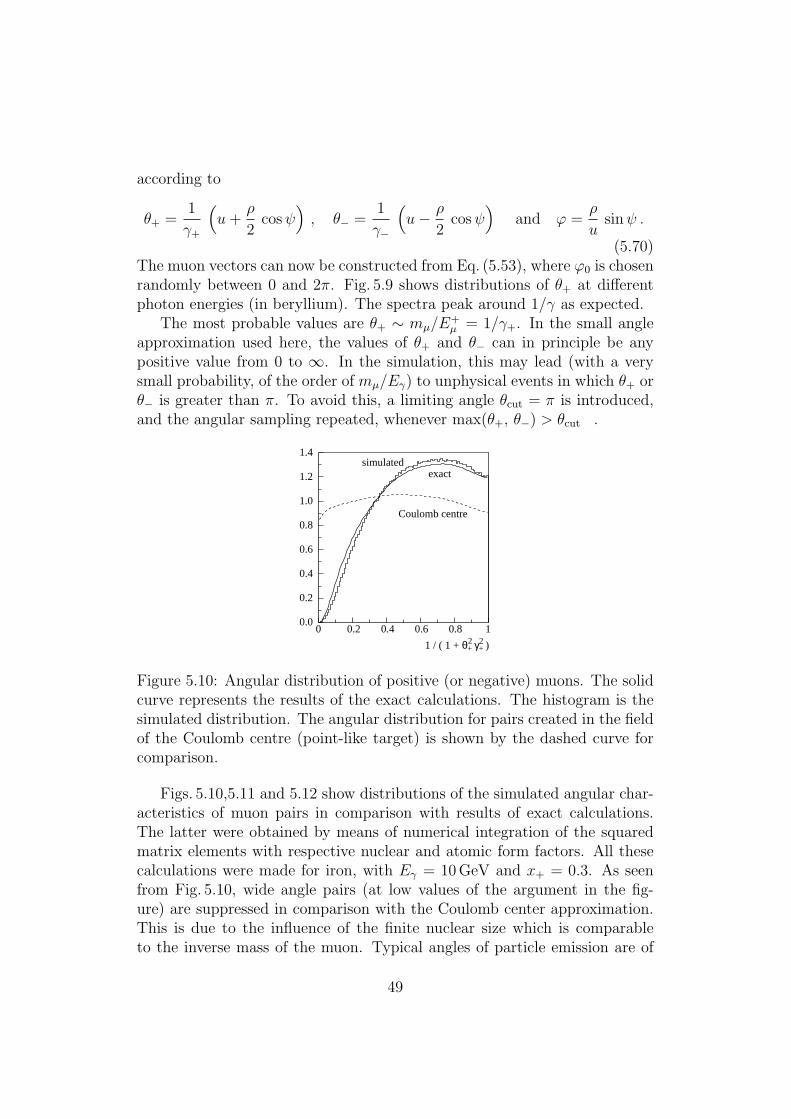
according to

θ+ =1

γ+

(

u+ρ

2cosψ

)

, θ− =1

γ−

(

u− ρ

2cosψ

)

and ϕ =ρ

usinψ .

(5.70)The muon vectors can now be constructed from Eq. (5.53), where ϕ0 is chosenrandomly between 0 and 2π. Fig. 5.9 shows distributions of θ+ at differentphoton energies (in beryllium). The spectra peak around 1/γ as expected.

The most probable values are θ+ ∼ mµ/E+µ = 1/γ+. In the small angle

approximation used here, the values of θ+ and θ− can in principle be anypositive value from 0 to ∞. In the simulation, this may lead (with a verysmall probability, of the order of mµ/Eγ) to unphysical events in which θ+ orθ− is greater than π. To avoid this, a limiting angle θcut = π is introduced,and the angular sampling repeated, whenever max(θ+, θ−) > θcut .

0.0

0.2

0.4

0.6

0.8

1.0

1.2

1.4

0 0.2 0.4 0.6 0.8 1

Coulomb centre

exactsimulated

1 / ( 1 + θ+ γ+ )2 2

Figure 5.10: Angular distribution of positive (or negative) muons. The solidcurve represents the results of the exact calculations. The histogram is thesimulated distribution. The angular distribution for pairs created in the fieldof the Coulomb centre (point-like target) is shown by the dashed curve forcomparison.

Figs. 5.10,5.11 and 5.12 show distributions of the simulated angular char-acteristics of muon pairs in comparison with results of exact calculations.The latter were obtained by means of numerical integration of the squaredmatrix elements with respective nuclear and atomic form factors. All thesecalculations were made for iron, with Eγ = 10GeV and x+ = 0.3. As seenfrom Fig. 5.10, wide angle pairs (at low values of the argument in the fig-ure) are suppressed in comparison with the Coulomb center approximation.This is due to the influence of the finite nuclear size which is comparableto the inverse mass of the muon. Typical angles of particle emission are of

49

0

1

2

3

4

5

6

7

10 -1 1

θ+ γ+

Figure 5.11: Angular distribution in logarithmic scale. The curve corre-sponds to the exact calculations and the histogram is the simulated distri-bution.

0

1

2

3

4

10-3

10-2

10-1

1| θ+ γ+ - θ- γ- |

Figure 5.12: Distribution of the difference of transverse momenta of positiveand negative muons (with logarithmic x-scale).

50

the order of 1/γ± = mµ/E±µ (Fig. 5.11). Fig. 5.12 illustrates the influence of

the momentum transferred to the target on the angular characteristics of theproduced pair. In the frame of the often used model which neglects targetrecoil, the pair particles would be symmetric in transverse momenta, andcoplanar with the initial photon.

Bibliography

[1] H. Burkhardt, S. Kelner, and R. Kokoulin, Monte Carlo Generator forMuon Pair Production. CERN-SL-2002-016 (AP) and CLIC Note 511,May 2002.

[2] S.R. Kelner, R.P. Kokoulin, and A.A. Petrukhin, About cross sectionfor high energy muon bremsstrahlung. Moscow Phys. Eng. Inst. 024-95,1995. 31pp.

51

Chapter 6

Elastic scattering

52

6.1 Multiple Scattering

Elastic scattering of electrons and other charged particles is an importantcomponent of any transport code. Elastic cross section is huge when particleenergy decreases, so multiple scattering (MSC) approach should be intro-duced in order to have acceptable CPU performance of the simulation. Auniversal interface G4VMultipleScattering is used by all Geant4 MSC pro-cesses [1]:

• G4eMultipleScattering;

• G4hMultipleScattering;

• G4MuMultipleScattering.

For concrete simulation the G4VMscModel interface is used, which is anextension of the base G4VEmModel interface. The following models areavailable:

• G4UrbanMscModel - since Geant4 10.0 only one Urban model is avail-able and it is applicable to all types of particles;

• G4GoudsmitSaundersonModel - for electrons and positrons [2];

• G4LowEWentzelVIModel - for all particles with low-energy limit 10 eV;

• G4WentzelVIModel - for muons and hadrons, for muons should be in-cluded in Physics List together with G4CoulombScattering process, forhadrons large angle scattering is simulated by hadron elastic process.

The discussion on Geant4 MSC models is available in Ref.[3]. Below we willdescribe models developed by L. Urban [4], because these models are usedin many Geant4 applications and have general components reused by othermodels.

6.1.1 Introduction

MSC simulation algorithms can be classified as either detailed or condensed.In the detailed algorithms, all the collisions/interactions experienced by theparticle are simulated. This simulation can be considered as exact, it givesthe same results as the solution of the transport equation. However, it canbe used only if the number of collisions is not too large, a condition fulfilledonly for special geometries (such as thin foils, or low density gas). In solid

53

or liquid media the average number of collisions is very large and the de-tailed simulation becomes very inefficient. High energy simulation codes usecondensed simulation algorithms, in which the global effects of the collisionsare simulated at the end of a track segment. The global effects generallycomputed in these codes are the net energy loss, displacement, and changeof direction of the charged particle. The last two quantities are computedfrom MSC theories used in the codes and the accuracy of the condensedsimulations is limited by accuracy of MSC approximation.

Most particle physics simulation codes use the multiple scattering theo-ries of Moliere [5], Goudsmit and Saunderson [6] and Lewis [7]. The theoriesof Moliere and Goudsmit-Saunderson give only the angular distribution aftera step, while the Lewis theory computes the moments of the spatial distribu-tion as well. None of these MSC theories gives the probability distributionof the spatial displacement. Each of the MSC simulation codes incorporatesits own algorithm to determine the angular deflection, true path length cor-rection, and spatial displacement of the charged particle after a given step.These algorithms are not exact, of course, and are responsible for most ofthe uncertainties of the transport codes. Also due to inaccuracy of MSC thesimulation results can depend on the value of the step length and generallyuser has to select the value of the step length carefully.

A new class of MSC simulation, the mixed simulation algorithms (seee.g.[8]), appeared in the literature recently. The mixed algorithm simulatesthe hard collisions one by one and uses a MSC theory to treat the effects ofthe soft collisions at the end of a given step. Such algorithms can preventthe number of steps from becoming too large and also reduce the dependenceon the step length. Geant4 original implementation of a similar approach isrealized in G4WentzelVIModel [3].

The Urban MSC models used in Geant4 belongs to the class of condensedsimulations. Urban uses model functions to determine the angular and spatialdistributions after a step. The functions have been chosen in such a way asto give the same moments of the (angular and spatial) distributions as aregiven by the Lewis theory [7].

6.1.2 Definition of Terms

In simulation, a particle is transported by steps through the detector ge-ometry. The shortest distance between the endpoints of a step is calledthe geometrical path length, z. In the absence of a magnetic field, this is astraight line. For non-zero fields, z is the length along a curved trajectory.Constraints on z are imposed when particle tracks cross volume boundaries.The path length of an actual particle, however, is usually longer than the ge-

54

ometrical path length, due to multiple scattering. This distance is called thetrue path length, t. Constraints on t are imposed by the physical processesacting on the particle.

The properties of the MSC process are determined by the transport meanfree paths, λk, which are functions of the energy in a given material. Thek-th transport mean free path is defined as

1

λk= 2πna

∫ 1

−1

[1− Pk(cosχ)]dσ(χ)

dΩd(cosχ) (6.1)

where dσ(χ)/dΩ is the differential cross section of the scattering, Pk(cosχ)is the k-th Legendre polynomial, and na is the number of atoms per volume.

Most of the mean properties of MSC computed in the simulation codesdepend only on the first and second transport mean free paths. The meanvalue of the geometrical path length (first moment) corresponding to a giventrue path length t is given by

〈z〉 = λ1

[

1− exp

(

− t

λ1

)]

(6.2)

Eq. 6.2 is an exact result for the mean value of z if the differential crosssection has axial symmetry and the energy loss can be neglected. The trans-formation between true and geometrical path lengths is called the path lengthcorrection. This formula and other expressions for the first moments of thespatial distribution were taken from either [8] or [9], but were originally cal-culated by Goudsmit and Saunderson [6] and Lewis [7].

At the end of the true step length, t, the scattering angle is θ. The meanvalue of cosθ is

〈cosθ〉 = exp

[

− t

λ1

]

(6.3)

The variance of cosθ can be written as

σ2 = 〈cos2θ〉 − 〈cosθ〉2 = 1 + 2e−2κτ

3− e−2τ (6.4)

where τ = t/λ1 and κ = λ1/λ2. The mean lateral displacement is givenby a more complicated formula [8], but this quantity can also be calculatedrelatively easily and accurately. The square of the mean lateral displacementis

〈x2 + y2〉 = 4λ213

[

τ − κ+ 1

κ+

κ

κ− 1e−τ − 1

κ(κ− 1)e−κτ

]

(6.5)

55

Here it is assumed that the initial particle direction is parallel to the the zaxis. The lateral correlation is determined by the equation

〈xvx + yvy〉 =2λ13

[

1− κ

κ− 1e−τ +

1

κ− 1e−κτ

]

(6.6)

where vx and vy are the x and y components of the direction unit vector. Thisequation gives the correlation strength between the final lateral position andfinal direction.

The transport mean free path values have been calculated in Refs.[10],[11]for electrons and positrons in the kinetic energy range 100 eV - 20 MeV in15 materials. The Urban MSC model in Geant4 uses these values for kineticenergies below 10 MeV. For high energy particles (above 10 MeV) the trans-port mean free path values have been taken from a paper of R. Mayol andF. Salvat [12]. When necessary, the model linearly interpolates or extrap-olates the transport cross section, σ1 = 1/λ1, in atomic number Z and inthe square of the particle velocity, β2. The ratio κ is a very slowly varyingfunction of the energy: κ > 2 for T > a few keV, and κ → 3 for very highenergies (see [9]). Hence, a constant value of 2.5 is used in the model.

Nuclear size effects are negligible for low energy particles and they areaccounted for in the Born approximation in [12], so there is no need for extracorrections of this kind in the Urban model.

6.1.3 Path Length Correction

As mentioned above, the path length correction refers to the transformationt −→ g and its inverse. The t −→ g transformation is given by Eq. 6.2 if thestep is small and the energy loss can be neglected. If the step is not smallthe energy dependence makes the transformation more complicated. For thiscase Eqs. 6.3,6.2 should be modified as

〈cosθ〉 = exp

[

−∫ t

0

du

λ1(u)

]

(6.7)

〈z〉 =∫ t

0

〈cosθ〉u du (6.8)

where θ is the scattering angle, t and z are the true and geometrical pathlengths, and λ1 is the transport mean free path.

In order to compute Eqs. 6.7,6.8 the t dependence of the transport meanfree path must be known. λ1 depends on the kinetic energy of the particle

56

which decreases along the step. All computations in the model use a linearapproximation for this t dependence:

λ1(t) = λ10(1− αt) (6.9)

Here λ10 denotes the value of λ1 at the start of the step, and α is a constant.It is worth noting that Eq. 6.9 is not a crude approximation. It is rathergood at low (< 1 MeV) energy. At higher energies the step is generally muchsmaller than the range of the particle, so the change in energy is small andso is the change in λ1. Using Eqs. 6.7 - 6.9 the explicit formula for 〈cosθ〉and 〈z〉 are:

〈cosθ〉 = (1− αt)1

αλ10 (6.10)

〈z〉 = 1

α(1 + 1αλ10

)

[

1− (1− αt)1+ 1

αλ10

]

(6.11)

The value of the constant α can be expressed using λ10 and λ11 where λ11 isthe value of the transport mean free path at the end of the step

α =λ10 − λ11tλ10

(6.12)

At low energies ( Tkin < M , M - particle mass) α has a simpler form:

α =1

r0(6.13)

where r0 denotes the range of the particle at the start of the step. It caneasily be seen that for a small step (i.e. for a step with small relative energyloss) the formula of 〈z〉 is

〈z〉 = λ10

[

1− exp

(

− t

λ10

)]

(6.14)

Eq. 6.11 or 6.14 gives the mean value of the geometrical step length for agiven true step length. The actual geometrical path length is sampled inthe model according to the simple probability density function defined forv = z/t ∈ [0, 1] :

f(v) = (k + 1)(k + 2)vk(1− v) (6.15)

The value of the exponent k is computed from the requirement that f(v)must give the same mean value for z = vt as Eq. 6.11 or 6.14. Hence

k =3〈z〉 − t

t− 〈z〉 (6.16)

57

The value of z = vt is sampled using f(v) if k > 0, otherwise z = 〈z〉 isused. The g −→ t transformation is performed using the mean values. Thetransformation can be written as

t(z) = 〈t〉 = −λ1 log(

1− z

λ1

)

(6.17)

if the geometrical step is small and

t(z) =1

α

[

1− (1− αwz)1w

]

(6.18)

where

w = 1 +1

αλ10if the step is not small, i.e. the energy loss should be taken into account.

6.1.4 Angular Distribution

The quantity u = cosθ is sampled according to a model function g(u). Theshape of this function has been chosen such that Eqs. 6.3 and 6.4 are satisfied.The functional form of g is

g(u) = q[pg1(u) + (1− p)g2(u)] + (1− q)g3(u) (6.19)

where 0 ≤ p, q ≤ 1, and the gi are simple functions of u = cosθ, normalizedover the range u ∈ [−1, 1]. The functions gi have been chosen as

g1(u) = C1 e−a(1−u) − 1 ≤ u0 ≤ u ≤ 1 (6.20)

g2(u) = C21

(b− u)d− 1 ≤ u ≤ u0 ≤ 1 (6.21)

g3(u) = C3 − 1 ≤ u ≤ 1 (6.22)

where a > 0, b > 0, d > 0 and u0 are model parameters, and the Ci arenormalization constants. It is worth noting that for small scattering angles,θ, g1(u) is nearly Gaussian (exp(−θ2/2θ20)) if θ20 ≈ 1/a, while g2(u) has aRutherford-like tail for large θ, if b ≈ 1 and d is not far from 2 .

6.1.5 Determination of the Model Parameters

The parameters a, b, d, u0 and p, q are not independent. The requirementthat the angular distribution function g(u) and its first derivative be contin-uous at u = u0 imposes two constraints on the parameters:

p g1(u0) = (1− p) g2(u0) (6.23)

58

p a g1(u0) = (1− p)d

b− u0g2(u0) (6.24)

A third constraint comes from Eq. 6.7 : g(u) must give the same mean valuefor u as the theory. It follows from Eqs. 6.10 and 6.19 that

qp〈u〉1 + (1− p)〈u〉2 = [1− α t]1

αλ10 (6.25)

where 〈u〉i denotes the mean value of u computed from the distribution gi(u).The parameter a was chosen according to a modified Highland-Lynch-Dahlformula for the width of the angular distribution [13], [14].

a =0.5

1− cos(θ0)(6.26)

where θ0 is

θ0 =13.6MeV

βcpzch

√

t

X0

[

1 + hc ln

(

t

X0

) ]

(6.27)

when the original Highland-Lynch-Dahl formula is used. Here θ0 = θrmsplane

is the width of the approximate Gaussian projected angle distribution, p,βc and zch are the momentum, velocity and charge number of the incidentparticle, and t/X0 is the true path length in radiation length unit. Thecorrection term hc = 0.038 in the formula. This value of θ0 is from a fit tothe Moliere distribution for singly charged particles with β = 1 for all Z,and is accurate to 11 % or better for 10−3 ≤ t/X0 ≤ 100 (see e.g. Rev. ofParticle Properties, section 23.3).

The model uses a slightly modified Highland-Lynch-Dahl formula to com-pute θ0. For electrons/positrons the modified θ0 formula is

θ0 =13.6MeV

βcpzch

√yc (6.28)

where

y = ln

(

t

X0

)

(6.29)

The correction term c and coeffitients ci are

c = c0(c1 + c2y), (6.30)

c0 = 0.990395− 0.168386Z1/6 + 0.093286Z1/3, (6.31)

c1 = 1− 0.08778

Z, (6.32)

59

c2 = 0.04078 + 0.00017315Z. (6.33)

This formula gives a much smaller step dependence in the angular dis-tribution than the Highland form. The value of the parameter u0 has beenchosen as

u0 = 1− ξ

a(6.34)

whereξ = d1 + d2v + d3v

2 + d4v3 (6.35)

with

v = ln

(

t

λ1

)

(6.36)

The parameters di-s have the form

di = di0 + di1Z13 + di2Z

23 (6.37)

The numerical values of the dij constants can be found in the code.The tail parameter d is the same as the parameter ξ .This (empirical) expression is obtained comparing the simulation results

to the data of the MuScat experiment [16]. The remaining three parame-ters can be computed from Eqs. 6.23 - 6.25. The numerical value of theparameters can be found in the code.

In the case of heavy charged particles (µ, π, p, etc.) the mean transportfree path is calculated from the electron or positron λ1 values with a ’scaling’applied. This is possible because the transport mean free path λ1 dependsonly on the variable Pβc, where P is the momentum, and βc is the velocityof the particle.

In its present form the model samples the path length correction and an-gular distribution from model functions, while for the lateral displacementand the lateral correlation only the mean values are used and all the othercorrelations are neglected. However, the model is general enough to incorpo-rate other random quantities and correlations in the future.

6.1.6 Step Limitation Algorithm

In Geant4 the boundary crossing is treated by the transportation process.The transportation ensures that the particle does not penetrate in a newvolume without stopping at the boundary, it restricts the step size when theparticle leaves a volume. However, this step restriction can be rather weakin big volumes and this fact can result a not very good angular distributionafter the volume. At the same time, there is no similar step limitation when

60

a particle enters a volume and this fact does not allow a good backscatteringsimulation for low energy particles. Low energy particles penetrate too deeplyinto the volume in the first step and then - because of energy loss - they arenot able to reach again the boundary in backward direction.

MSC step limitation algorithm has been developed [4] in order to achieveoptimal balance between simulation precision and CPU performance of sim-ulation for different applications. At the start of a track or after entering ina new volume, the algorithm restricts the step size to a value

fr ·maxr, λ1 (6.38)

where r is the range of the particle, fr is a parameter ∈ [0, 1], taking the maxof r and λ1 is an empirical choice.The value of fr is constant for low energyparticles while for particles with λ1 > λlim an effective value is used given bythe scaling equation

freff = fr ·[

1− sc+ sc ∗ λ1λlim

]

(6.39)

( The numerical values sc = 0.25 and λlim = 1 mm are used in the equation.)In order not to use very small - unphysical - step sizes a lower limit is givenfor the step size as

tlimitmin = max

[

λ1nstepmax

, λelastic

]

(6.40)

with nstepmax = 25 and λelastic is the elastic mean free path of the particle(see later).

It can be easily seen that this kind of step limitation poses a real constraintonly for low energy particles. In order to prevent a particle from crossing avolume in just one step, an additional limitation is imposed: after enteringa volume the step size cannot be bigger than

dgeomfg

(6.41)

where dgeom is the distance to the next boundary (in the direction of theparticle) and fg is a constant parameter. A similar restriction at the start ofa track is

2dgeomfg

(6.42)

At this point the program also checks whether the particle has entered anew volume. If it has, the particle steps cannot be bigger than tlim =

61

fr max(r, λ). This step limitation is governed by the physics, because tlimdepends on the particle energy and the material.

The choice of the parameters fr and fg is also related to performance.By default fr = 0.02 and fg = 2.5 are used, but these may be set to anyother value in a simple way. One can get an approximate simulation ofthe backscattering with the default value, while if a better backscatteringsimulation is needed it is possible to get it using a smaller value for fr.However, this model is very simple and it can only approximately reproducethe backscattering data.

6.1.7 Boundary Crossing Algorithm

A special stepping algorithm has been implemented in order to improve thesimulation around interfaces. This algorithm does not allow ’big’ last stepsin a volume and ’big’ first steps in the next volume. The step length of thesesteps around a boundary crossing can not be bigger than the mean free pathof the elastic scattering of the particle in the given volume (material). Afterthese small steps the particle scattered according to a single scattering law(i.e. there is no multiple scattering very close to the boundary or at theboundary).

The key parameter of the algorithm is the variable called skin. Thealgorithm is not active for skin ≤ 0, while for skin > 0 it is active inlayers of thickness skin · λelastic before boundary crossing and of thickness(skin−1)·λelastic after boundary crossing (for skin = 1 there is only one smallstep just before the boundary). In this active area the particle performs stepsof length λelastic (or smaller if the particle reaches the boundary traversing asmaller distance than this value).

The scattering at the end of a small step is single or plural and for thesesmall steps there are no path length correction and lateral displacement com-putation. In other words the program works in this thin layer in ’microscopicmode’. The elastic mean free path can be estimated as

λelastic = λ1 · rat (Tkin) (6.43)

where rat(Tkin) a simple empirical function computed from the elastic andfirst transport cross section values of Mayol and Salvat [12]

rat (Tkin) =0.001(MeV )2

Tkin (Tkin + 10MeV )(6.44)

Tkin is the kinetic energy of the particle.At the end of a small step the number of scatterings is sampled according

to the Poisson’s distribution with a mean value t/λelastic and in the case of

62

plural scattering the final scattering angle is computed by summing the con-tributions of the individual scatterings. The single scattering is determinedby the distribution

g(u) = C1

(2a+ 1− u)2(6.45)

where u = cos(θ) , a is the screening parameter, C is a normalization con-stant. The form of the screening parameter is the same as in the singlescattering (see there).

6.1.8 Implementation Details

The step length of a particles is determined by the physics processes or thegeometry of the detectors. The tracking/stepping algorithm checks all thestep lengths demanded by the (continuous or discrete) physics processes anddetermines the minimum of these step lengths (see 3.1). The MSC modelshould be called to compute step limit after all processes except the trans-portation process. The following sequence of computations are performed tomake the step:

• the minimum of all processes true step length limit t including one ofthe MSC process is selected;

• The conversion t −→ g (geometrical step limit) is performed;

• the minimum of obtained value g and the transportation step limit isselected;

• The final conversion g −→ t is performed.

The reason for this ordering is that the physics processes ’feel’ the true pathlength t traveled by the particle, while the transportation process (geometry)uses the z step length.

A new optional mechanis was recently introduced allowing sample dis-placemnt in vicinity of geometry boundary. If it is enabled and the trans-portation limit the step due to geometry boundary then after initial samplingof the displacenet an additional ’push’ of track is applied forcing end point beat the boundary. Corresponding correction to the true step length is appliedaccording to the value of the ’push’.

After the actual step of the particle is done, the MSC model is responsiblefor sampling of scattering angle and relocation of the end-point of the step.The scattering angle θ of the particle after the step of length ’t’ is sampledaccording to the model function given in Eq. 6.19 . The azimuthal angle φis generated uniformly in the range [0, 2π].

63

After the simulation of the scattering angle, the lateral displacement iscomputed using Eq. 6.5. Then the correlation given by Eq. 6.6 is used todetermine the direction of the lateral displacement. Before ’moving’ theparticle according to the displacement a check is performed to ensure thatthe relocation of the particle with the lateral displacement does not take theparticle beyond the volume boundary.

Default MSC parameter values optimized per particle type are shown inTable 6.1. Note, that there is three types of step limitation by multiplescattering process:

• Minimal - only fr parameter and range are used;

• UseSafety - fr parameter, range and geometrical safety are used;

• UseSafetyPlus - fr parameter, range and geometrical safety are used;

• UseDistanceToBoundary - uses particle range, geometrical safety andlinear distance to geometrical boundary.

particle e+, e− muons, hadrons ionsStepLimitType fUseSafety fMinimal fMinimal

skin 0 0 0fr 0.04 0.2 0.2fg 2.5 0.1 0.1

LateralDisplacement true true false

Table 6.1: The default values of parameters for different particle type.

The parameters of the model can be changed via public functions of the baseclass G4VMultipleSacttering. They can be changed for all multiple scatteringprocesses simultaneously via G4EmParameters class, G4EmProcessOptionsclass, or via Geant4 UI commands. The following commands are available:

/process/msc/StepLimit UseDistanceToBoundary/process/msc/LateralDisplacement false/process/msc/MuHadLateralDisplacement false/process/msc/DisplacementBeyondSafety true/process/msc/RangeFactor 0.02/process/msc/GeomFactor 2.5/process/msc/Skin 2

64

Bibliography


[2] O. Kadri, V. Ivanchenko, F. Gharbi, A. Trabelsi, Incorporation of theGoudsmit-Saunderson electron transport theory in the Geant4 MonteCarlo code, Nucl. Instrum. and Meth. B 267 (2009) 3624.

[3] V.N. Ivanchenko et al., Geant4 models for simulation of multiple scat-tering, J. Phys.: Conf. Ser. 219 (2010) 032045.

[4] L. Urban, A multiple scattering model, CERN-OPEN-2006-077, Dec2006. 18 pp.

[5] G.Z. Moliere Z. Naturforsch. 3a (1948) 78.

[6] S. Goudsmit and J.L. Saunderson. Phys. Rev. 57 (1940) 24.

[7] H.W. Lewis. Phys. Rev. 78 (1950) 526.

[8] J.M. Fernandez-Varea et al. NIM B73 (1993) 447.

[9] I. Kawrakow and A.F. Bielajew NIM B 142 (1998) 253.

[10] D. Liljequist and M. Ismail. J.Appl.Phys. 62 (1987) 342.

[11] D. Liljequist et al. J.Appl.Phys. 68 (1990) 3061.

[12] R. Mayol and F. Salvat At.Data and Nucl.Data Tables 65 (1997) 55..

[13] V.L. Highland NIM 129 (1975) 497.

[14] G.R. Lynch and O.I. Dahl NIM B58 (1991) 6.

[15] G. Shen et al. Phys. Rev. D 20 (1979) 1584.

[16] D. Attwood et al. NIM B 251 (2006) 41.

65

6.2 Discrete Processes for Charged Particles

Some processes for charged particles following the same interfaceG4V EmProcessas gamma processes described in section 5.1:

• G4CoulombScattering;

• G4eplusAnnihilation (with additional AtRest methods);

• G4eplusPolarizedAnnihilation (with additional AtRest methods);

• G4eeToHadrons;

• G4NuclearStopping;

• G4MicroElecElastic;

• G4MicroElecInelastic.

Corresponding model classes follow the G4V EmModel interface:

• G4DummyModel (zero cross section, no secondaries);

• G4eCoulombScatteringModel;

• G4eSingleCoulombScatteringModel;

• G4IonCoulombScatteringModel;

• G4eeToHadronsModel;

• G4PenelopeAnnihilationModel;

• G4PolarizedAnnihilationModel;

• G4ICRU49NuclearStoppingModel;

• G4MicroElecElasticModel;

• G4MicroElecInelasticModel.

Some processes from do not follow described EM interfaces but provide directimplementations of the basic G4V DiscreteProcess process:

• G4AnnihiToMuPair;

• G4ScreenedNuclearRecoil;

66

• G4Cerenkov;

• G4Scintillation;

• G4SynchrotronRadiation;

67

6.3 Single Scattering

Single elastic scattering process is an alternative to the multiple scatteringprocess. The advantage of the single scattering process is in possibility ofusage of theory based cross sections, in contrary to the Geant4 multiple scat-tering model [1], which uses a number of phenomenological approximationson top of Lewis theory. The process G4CoulombScattering was created forsimulation of single scattering of muons, it also applicable with some physicallimitations to electrons, muons and ions. Because each of elastic collisions aresimulated the number of steps of charged particles significantly increasing incomparison with the multiple scattering approach, correspondingly its CPUperformance is pure. However, in low-density media (vacuum, low-densitygas) multiple scattering may provide wrong results and single scattering pro-cesses is more adequate.

6.3.1 Coulomb Scattering

The single scattering model of Wentzel [2] is used in many of multiple scat-tering models including Penelope code [4]. The Wentzel for describing elasticscattering of particles with charge ze (z = −1 for electron) by atomic nucleuswith atomic number Z based on simplified scattering potential

V (r) =zZe2

rexp(−r/R), (6.46)

where the exponential factor tries to reproduce the effect of screening. Theparameter R is a screening radius [3]

R = 0.885Z−1/3rB, (6.47)

where rB is the Bohr radius. In the first Born approximation the elasticscattering cross section σ(W ) can be obtained as

dσ(W )(θ)

dΩ=

(ze2)2

(pβc)2Z(Z + 1)

(2A+ 1− cosθ)2, (6.48)

where p is the momentum and β is the velocity of the projectile particle. Thescreening parameter A according to Moliere and Bethe [3]

A =

(

ℏ

2pR

)2

(1.13 + 3.76(αZ/β)2), (6.49)

where α is a fine structure constant and the factor in brackets is used to takeinto account second order corrections to the first Born approximation.

68

The total elastic cross section σ can be expressed via Wentzel cross section(6.48)

dσ(θ)

dΩ=dσ(W )(θ)

dΩ

(

Z

(1 + (qRN )2

12)2

+ 1

)

1

Z + 1, (6.50)

where q is momentum transfer to the nucleus, RN is nuclear radius. Thisterm takes into account nuclear size effect [5], the second term takes intoaccount scattering off electrons. The results of simulation with the singlescattering model (Fig.6.1) are competitive with the results of the multiplescattering.

Figure 6.1: Scattering of muons off 1.5 mm aluminum foil: data [6] - blacksquares; simulation - colored markers corresponding different options of mul-tiple scattering and single scattering model; in the bottom plot - relativedifference between the simulation and the data in percents; hashed areademonstrates one standard deviation of the data.


The total cross section of the process is obtained as a result of integrationof the differential cross section (6.50). The first term of this cross sectionis integrated in the interval (0, π). The second term in the smaller interval(0, θm), where θm is the maximum scattering angle off electrons, which isdetermined using the cut value for the delta electron production. Before

69

sampling of angular distribution the random choice is performed betweenscattering off the nucleus and off electrons.

Bibliography

[1] L. Urban, A multiple scattering model, CERN-OPEN-2006-077, Dec2006. 18 pp.

[2] G. Wentzel, Z. Phys. 40 (1927) 590.

[3] H.A. Bethe, Phys. Rev. 89 (1953) 1256.

[4] J.M. Fernandez-Varea et al. NIM B 73 (1993) 447.

[5] A.V. Butkevich et al., NIM A 488 (2002) 282.

[6] D. Attwood et al. NIM B 251 (2006) 41.

70

6.4 Ion Scattering

The necessity of accurately computing the characteristics of interatomic scat-tering arises in many disciplines in which energetic ions pass through mate-rials. Traditionally, solutions to this problem not involving hadronic inter-actions have been dominated by the multiple scattering, which is reasonablysuccessful, but not very flexible. In particular, it is relatively difficult to in-troduce into such a system a particular screening function which has beenmeasured for a specific atomic pair, rather than the universal functions whichare applied. In many problems of current interest, such as the behavior ofsemiconductor device physics in a space environment, nuclear reactions, par-ticle showers, and other effects are critically important in modeling the fulldetails of ion transport. The process G4ScreenedNuclearRecoil provides sim-ulation of ion elastic scattering [1]. This process is available with extendedelectromagnetic example TestEm7.

6.4.1 Method

The method used in this computation is a variant of a subset of the methoddescribed in Ref.[2]. A very short recap of the basic material is included here.The scattering of two atoms from each other is assumed to be a completelyclassical process, subject to an interatomic potential described by a potentialfunction

V (r) =Z1Z2e

2

rφ(r

a

)

(6.51)

where Z1 and Z2 are the nuclear proton numbers, e2 is the electromagneticcoupling constant (q2e/4πǫ0 in SI units), r is the inter-nuclear separation, φis the screening function describing the effect of electronic screening of thebare nuclear charges, and a is a characteristic length scale for this screening.In most cases, φ is a universal function used for all ion pairs, and the value ofa is an appropriately adjusted length to give reasonably accurate scatteringbehavior. In the method described here, there is no particular need fora universal function φ, since the method is capable of directly solving theproblem for most physically plausible screening functions. It is still usefulto define a typical screening length a in the calculation described below, tokeep the equations in a form directly comparable with our previous work eventhough, in the end, the actual value is irrelevant as long as the final functionφ(r) is correct. From this potential V (r) one can then compute the classicalscattering angle from the reduced center-of-mass energy ε ≡ Eca/Z1Z2e

2

(where Ec is the kinetic energy in the center-of-mass frame) and reduced

71

impact parameter β ≡ b/a

θc = π − 2β

∫ ∞

x0

f(z) dz/z2 (6.52)

where

f(z) =

(

1− φ(z)

z ε− β2

z2

)−1/2

(6.53)

and x0 is the reduced classical turning radius for the given ε and β.The problem, then, is reduced to the efficient computation of this scat-

tering integral. In our previous work, a great deal of analytical effort wasincluded to proceed from the scattering integral to a full differential crosssection calculation, but for application in a Monte-Carlo code, the scatteringintegral θc(Z1, Z2, Ec, b) and an estimated total cross section σ0(Z1, Z2, Ec)are all that is needed. Thus, we can skip algorithmically forward in the orig-inal paper to equations 15-18 and the surrounding discussion to compute thereduced distance of closest approach x0. This computation follows that inthe previous work exactly, and will not be reintroduced here.

For the sake of ultimate accuracy in this algorithm, and due to the rela-tively low computational cost of so doing, we compute the actual scatteringintegral (as described in equations 19-21 of [2]) using a Lobatto quadratureof order 6, instead of the 4th order method previously described. This re-sults in the integration accuracy exceeding that of any available interatomicpotentials in the range of energies above those at which molecular structureeffects dominate, and should allow for future improvements in that area. Theintegral α then becomes (following the notation of the previous paper)

α ≈ 1 + λ0

30+

4∑

i=1

w′i f

(

x0

qi

)

(6.54)

where

λ0 =

(

1

2+

β2

2x20− φ′(x0)

2 ε

)−1/2

(6.55)

w′i ∈[0.03472124, 0.1476903, 0.23485003, 0.1860249]

qi ∈[0.9830235, 0.8465224, 0.5323531, 0.18347974]Then

θc = π − πβα

x0

(6.56)

The other quantity required to implement a scattering process is the totalscattering cross section σ0 for a given incident ion and a material through

72

which the ion is propagating. This value requires special consideration for aprocess such as screened scattering. In the limiting case that the screeningfunction is unity, which corresponds to Rutherford scattering, the total crosssection is infinite. For various screening functions, the total cross sectionmay or may not be finite. However, one must ask what the intent of defininga total cross section is, and determine from that how to define it.

In Geant4, the total cross section is used to determine a mean-free-pathlµ which is used in turn to generate random transport distances betweendiscrete scattering events for a particle. In reality, where an ion is propagatingthrough, for example, a solid material, scattering is not a discrete processbut is continuous. However, it is a useful, and highly accurate, simplificationto reduce such scattering to a series of discrete events, by defining someminimum energy transfer of interest, and setting the mean free path to bethe path over which statistically one such minimal transfer has occurred. Thisapproach is identical to the approach developed for the original TRIM code[3]. As long as the minimal interesting energy transfer is set small enoughthat the cumulative effect of all transfers smaller than that is negligible,the approximation is valid. As long as the impact parameter selection isadjusted to be consistent with the selected value of lµ, the physical resultisn’t particularly sensitive to the value chosen.

Noting, then, that the actual physical result isn’t very sensitive to theselection of lµ, one can be relatively free about defining the cross section σ0

from which lµ is computed. The choice used for this implementation is fairlysimple. Define a physical cutoff energy Emin which is the smallest energytransfer to be included in the calculation. Then, for a given incident particlewith atomic number Z1, mass m1, and lab energy Einc, and a target atomwith atomic number Z2 and mass m2, compute the scattering angle θc whichwill transfer this much energy to the target from the solution of

Emin = Einc4m1m2

(m1 +m2)2sin2 θc

2(6.57)

. Then, noting that α from eq. 6.54 is a number very close to unity, onecan solve for an approximate impact parameter b with a single root-findingoperation to find the classical turning point. Then, define the total crosssection to be σ0 = πb2, the area of the disk inside of which the passage of anion will cause at least the minimum interesting energy transfer. Because thisprocess is relatively expensive, and the result is needed extremely frequently,the values of σ0(Einc) are precomputed for each pairing of incident ion andtarget atom, and the results cached in a cubic-spline interpolation table.However, since the actual result isn’t very critical, the cached results can bestored in a very coarsely sampled table without degrading the calculation at

73

all, as long as the values of the lµ used in the impact parameter selection arerigorously consistent with this table.

The final necessary piece of the scattering integral calculation is the sta-tistical selection of the impact parameter b to be used in each scatteringevent. This selection is done following the original algorithm from TRIM,where the cumulative probability distribution for impact parameters is

P (b) = 1− exp

(−π b2σ0

)

(6.58)

where N σ0 ≡ 1/lµ where N is the total number density of scattering centersin the target material and lµ is the mean free path computed in the conven-tional way. To produce this distribution from a uniform random variate r on(0,1], the necessary function is

b =

√

− log r

π N lµ(6.59)

This choice of sampling function does have the one peculiarity that it canproduce values of the impact parameter which are larger than the impactparameter which results in the cutoff energy transfer, as discussed abovein the section on the total cross section, with probability 1/e. When thisoccurs, the scattering event is not processed further, since the energy transferis below threshold. For this reason, impact parameter selection is carried outvery early in the algorithm, so the effort spent on uninteresting events isminimized.

The above choice of impact sampling is modified when the mean-free-path

is very short. If σ0 > π(

l2

)2where l is the approximate lattice constant of

the material, as defined by l = N−1/3, the sampling is replaced by uniformsampling on a disk of radius l/2, so that

b =l

2

√r (6.60)

This takes into account that impact parameters larger than half the latticespacing do not occur, since then one is closer to the adjacent atom. This alsoderives from TRIM.

One extra feature is included in our model, to accelerate the produc-tion of relatively rare events such as high-angle scattering. This feature is across-section scaling algorithm, which allows the user access to an unphys-ical control of the algorithm which arbitrarily scales the cross-sections fora selected fraction of interactions. This is implemented as a two-parameter

74

adjustment to the central algorithm. The first parameter is a selection fre-quency fh which sets what fraction of the interactions will be modified. Thesecond parameter is the scaling factor for the cross-section. This is imple-mented by, for a fraction fh of interactions, scaling the impact parameter byb′ = b/

√scale. This feature, if used with care so that it does not provide

excess multiple-scattering, can provide between 10 and 100-fold improve-ments to event rates. If used without checking the validity by comparing toun-adjusted scattering computations, it can also provide utter nonsense.


The coefficients for the summation to approximate the integral for α ineq.(6.54) are derived from the values in Abramowitz & Stegun [4], altered tomake the change-of-variable used for this integral. There are two basic stepsto the transformation. First, since the provided abscissas xi and weights wi

are for integration on [-1,1], with only one half of the values provided, andin this work the integration is being carried out on [0,1], the abscissas aretransformed as:

yi ∈

1∓ xi2

(6.61)

Then, the primary change-of-variable is applied resulting in:

qi = cosπ yi2

(6.62)

w′i =

wi

2sin

π yi2

(6.63)

except for the first coefficient w′1where the sin() part of the weight is taken

into the limit of λ0 as described in eq.(6.55). This value is just w′1 = w1/2.

Bibliography

[1] M.H. Mendenhall, R.A. Weller, An algorithm for computing screenedCoulomb scattering in Geant4, Nucl. Instr. Meth. B 227 (2005) 420.

[2] M.H. Mendenhall, R.A. Weller, Algorithms for the rapid computationof classical cross sections for screened coulomb collisions, Nucl. Instr.Meth. in Physics Res. B58 (1991) 11.

[3] J.P. Biersack, L.G. Haggmark, A Monte Carlo computer program forthe transport of energetic ions in amorphous targets, Nucl. Instr. Meth.in Physics Res. 174 (1980) 257.

75

[4] M. Abramowitz, I. Stegun (Eds.), Handbook of Mathematical Functions,Dover, New York, 1965, pp. 888, 920.

76

6.5 Single Scattering, Screened Coulomb Po-

tential and NIEL

Alternative model of Coulomb scattering of ions have been developed basedon [1] and references therein. The advantage of this model is the wide appli-cability range in energy from 50 keV to 100 TeV per nucleon.

6.5.1 Nucleus–Nucleus Interactions

As discussed in Ref. [1], at small distances from the nucleus, the potentialenergy is a Coulomb potential, while - at distances larger than the Bohrradius - the nuclear field is screened by the fields of atomic electrons. Theinteraction between two nuclei is usually described in terms of an interatomicCoulomb potential (e.g., see Section 2.1.4.1 of Ref. [2] and Section 4.1 ofRef. [3]), which is a function of the radial distance r between the two nuclei

V (r) =zZe2

rΨI(rr), (6.64)

where ez (projectile) and eZ (target) are the charges of the bare nuclei andΨI is the interatomic screening function and rr is given by

rr =r

aI, (6.65)

with aI the so-called screening length (also termed screening radius). In theframework of the Thomas–Fermi model of the atom (e.g., see Ref. [1] andreferences therein) - thus, following the approach of ICRU Report 49 (1993)-, a commonly used screening length for z = 1 incoming particles is that fromThomas–Fermi

aTF =CTF a0Z1/3

, (6.66)

and - for incoming particles with z ≥ 2 - that introduced by Ziegler, Biersackand Littmark (1985) (and termed universal screening length):

aU =CTF a0

z0.23 + Z0.23, (6.67)

where

a0 =~2

me2

is the Bohr radius, m is the electron rest mass and

CTF =1

2

(

3 π

4

)2/3

≃ 0.88534

77

is a constant introduced in the Thomas–Fermi model.The simple scattering model due to Wentzel [5] - with a single exponen-

tial screening-function ΨI(rr) e.g., see Ref. [1] and references therein - wasrepeatedly employed in treating single and multiple Coulomb-scattering withscreened potentials. The resulting elastic differential cross section differs fromthe Rutherford differential cross section by an additional term - the so-calledscreening parameter - which prevents the divergence of the cross section whenthe angle θ of scattered particles approaches 0. The screening parameter As

[e.g., see Equation (21) of Bethe (1953)] - as derived by Moliere (1947, 1948)for the single Coulomb scattering using a Thomas–Fermi potential - is ex-pressed as

As =

(

~

2 p aI

)2[

1.13 + 3.76×(

αzZ

β

)2]

(6.68)

where aI is the screening length - from Eqs. (6.66, 6.67) for particles withz = 1 and z ≥ 2, respectively; α is the fine-structure constant; p (βc) isthe momentum (velocity) of the incoming particle undergoing the scatteringonto a target supposed to be initially at rest; c and ~ are the speed of lightand the reduced Planck constant, respectively. When the (relativistic) mass- with corresponding rest mass m - of the incoming particle is much lowerthan the rest mass (M) of the target nucleus, the differential cross section -obtained from the Wentzel–Moliere treatment of the single scattering - is:

dσWM(θ)

dΩ=

(

zZe2

2 p βc

)21

[

As + sin2(θ/2)]2 . (6.69)

Equation (6.69) differs from Rutherford’s formula - as already mentioned -for the additional term As to sin2(θ/2). As discussed in Ref. [1], for β ≃ 1(i.e., at very large p) and with As ≪ 1, one finds that the cross sectionapproaches a constant:

σWMc ≃

(

2 zZe2aI~c

)2π

1.13 + 3.76× (αzZ)2. (6.70)

As discussed in Ref. [1] and references therein, for a scattering under theaction of a central potential (for instance that due to a screened Coulombfield), when the rest mass of the target particle is no longer much larger thanthe relativistic mass of the incoming particle, the expression of the differentialcross section must properly be re-written - in the center of mass system - interms of an “effective particle” with momentum equal to that of the incomingparticle (p′in) and rest mass equal to the relativistic reduced mass

µrel =mM

M1,2

, (6.71)

78

whereM1,2 is the invariant mass;m andM are the rest masses of the incomingand target particles, respectively. The “effective particle” velocity is given by:

βrc = c

√

√

√

√

[

1 +

(

µrelc

p′in

)2]−1

.

Thus, one finds (e.g, see Ref. [1]):

dσWM(θ′)

dΩ′ =

(

zZe2

2 p′in βrc

)21

[

As + sin2(θ′/2)]2 , (6.72)

with

As =

(

~

2 p′in aI

)2[

1.13 + 3.76×(

αzZ

βr

)2]

(6.73)

and θ′ the scattering angle in the center of mass system.The energy T transferred to the recoil target is related to the scattering

angle as T = Tmax sin2 (θ′/2) - where Tmax is the maximum energy which

can be transferred in the scattering (e.g., see Section 1.5 of Ref. [2]) -, thus,assuming an isotropic azimuthal distribution one can re-write Eq. (6.72) interms of the kinetic recoil energy T of the target

dσWM(T )

dT= π

(

zZe2

p′in βrc

)2Tmax

[TmaxAs + T ]2. (6.74)

Furthermore, one can demonstrates that Eq. (6.74) can be re-written as(e.g, see Ref. [1]);

dσWM(T )

dT= 2 π

(

zZe2)2 E2

p2Mc41

[TmaxAs + T ]2(6.75)

with p and E the momentum and total energy of the incoming particle in thelaboratory. Equation (6.75) expresses - as already mentioned - the differentialcross section as a function of the (kinetic) energy T achieved by the recoiltarget.

6.5.2 Nuclear Stopping Power

Using Eq. (6.75) the nuclear stopping power - in MeV cm−1 - is obtained as

−(

dE

dx

)

nucl

= 2nAπ(

zZe2)2 E2

p2Mc4

[

As

As + 1− 1 + ln

(

As + 1

As

)]

(6.76)

79

10-1 100 101 102 103 104 105 106 107 10810-4

10-3

10-2

10-1

100

101

102

103

104

proton

208Pb115In56Fe28Si

12C11B

Stop

ping

pow

er

[MeV

cm

2 g-1

]

Kinetic Energy [MeV/nucleon]

alpha

in silicon

Figure 6.2: Nuclear stopping power from Ref. [1] - in MeV cm2 g−1 - calcu-lated using Eq. (6.76) in silicon is shown as a function of the kinetic energy pernucleon - from 50 keV/nucleon up 100TeV/nucleon - for protons, α-particleand 11B-, 12C-, 28Si-, 56Fe-, 115In-, 208Pb-nuclei.

with nA the number of nuclei (atoms) per unit of volume and, finally, thenegative sign indicates that the energy is lost by the incoming particle (thus,achieved by recoil targets). As discussed in Ref. [1], a slight increase of thenuclear stopping power with energy is expected because of the decrease ofthe screening parameter with energy.

For instance, in Fig. 6.2 the nuclear stopping power in silicon - in MeV cm2 g−1

- is shown as a function of the kinetic energy per nucleon - from 50 keV/nucleonup 100TeV/nucleon - for protons, α-particles and 11B-, 12C-, 28Si-, 56Fe-,115In-, 208Pb-nuclei.

A comparison of the present treatment with that obtained from Ziegler,Biersack and Littmark (1985) - available in SRIM (2008) [8] - using the so-called universal screening potential (see also Ref. [9]) is discussed in Ref. [1]:a good agreement is achieved down to about 150 keV/nucleon. At large en-ergies, the non-relativistic approach due to Ziegler, Biersack and Littmark(1985) becomes less appropriate and deviations from stopping powers cal-culated by means of the universal screening potential are expected and ob-served.

The non-relativistic approach - based on the universal screening potential- of Ziegler, Biersack and Littmark (1985) was also used by ICRU (1993) tocalculate nuclear stopping powers due to protons and α-particles in materi-als. ICRU (1993) used as screening lengths those from Eqs. (6.66, 6.67) forprotons and α-particles, respectively. As discussed in Ref. [1], the stoppingpowers for protons (α-particles) from Eq. (6.76) are less than ≈ 5% larger

80

10-1 100 101 102 103 104 105 106 107 108

10-4

10-3

10-2

10-1

100

101

102

103

proton

208Pb115In56Fe28Si

12C11B

NIE

L [M

eV c

m2 g-1

]

Kinetic Energy [MeV/nucleon]

alpha

in silicon

Figure 6.3: Non-ionizing stopping power from Ref. [1] - in MeV cm2 g−1 -calculated using Eq. (6.79) in silicon is shown as a function of the kineticenergy per nucleon - from 50 keV/nucleon up 100TeV/nucleon - for protons,α-particles and 11B-, 12C-, 28Si-, 56Fe-, 115In-, 208Pb-nuclei. The thresholdenergy for displacement is 21 eV in silicon.

than those reported by ICRU (1993) from 50 keV/nucleon up to ≈ 8MeV(19MeV/nucleon). At larger energies the stopping powers from Eq. (6.76)differ from those from ICRU - as expected - due to the complete relativistictreatment of the present approach (see Ref. [1]).

The simple screening parameter used so far [Eq. (6.73)] - derived byMoliere (1947) - can be modified by means of a practical correction, i.e.,

A′s =

(

~

2 p′in aI

)2[

1.13 + 3.76× C

(

αzZ

βr

)2]

, (6.77)

to achieve a better agreement with low energy calculations of Ziegler, Biersackand Littmark (1985). For instance - as discussed in Ref. [1] -, for α-particlesand heavier ions, with

C = (10πzZα)0.12 (6.78)

the stopping powers obtained from Eq. (6.76) - in which A′s replaces As - differ

from the values of SRIM (2008) by less than≈ 4.7 (3.6)% for α-particles (leadions) in silicon down to about 50 keV/nucleon. With respect to the tabulatedvalues of ICRU (1993), the agreement for α-particles is usually better than4% at low energy down to 50 keV/nucleon - a 5% agreement is achieved atabout 50 keV/nucleon in case of a lead medium. At very high energy, thestopping power is slightly affected when A′

s replaces As (a further disvussionis found in Ref. [1]).

81

6.5.3 Non-Ionizing Energy Loss due to Coulomb Scat-tering

A relevant process - which causes permanent damage to the silicon bulk struc-ture - is the so-called displacement damage (e.g., see Chapter 4 of Ref. [2],Ref. [10] and references therein). Displacement damage may be inflicted whena primary knocked-on atom (PKA) is generated. The interstitial atom andrelative vacancy are termed Frenkel-pair (FP). In turn, the displaced atommay have sufficient energy to migrate inside the lattice and - by further col-lisions - can displace other atoms as in a collision cascade. This displacementprocess modifies the bulk characteristics of the device and causes its degra-dation. The total number of FPs can be estimated calculating the energydensity deposited from displacement processes. In turn, this energy densityis related to the Non-Ionizing Energy Loss (NIEL), i.e., the energy per unitpath lost by the incident particle due to displacement processes.

In case of Coulomb scattering on nuclei, the non-ionizing energy-loss canbe calculated using the Wentzel–Moliere differential cross section [Eq. (6.75)]discussed in Sect. 6.5.1, i.e.,

−(

dE

dx

)NIEL

nucl

= nA

∫ Tmax

Td

T L(T )dσWM(T )

dTdT , (6.79)

where E is the kinetic energy of the incoming particle, T is the kinetic energytransferred to the target atom, L(T ) is the fraction of T deposited by meansof displacement processes. The expression of L(T ) - the so-called Lindhardpartition function - can be found, for instance, in Equations (4.94, 4.96) ofSection 4.2.1.1 in Ref. [2] (see also references therein). Tde = T L(T ) is theso-called damage energy, i.e., the energy deposited by a recoil nucleus withkinetic energy T via displacement damages inside the medium. The integral inEq. (6.79) is computed from the minimum energy Td - the so-called thresholdenergy for displacement, i.e., that energy necessary to displace the atom fromits lattice position - up to the maximum energy Tmax that can be transferredduring a single collision process. Td is about 21 eV in silicon. For instance, inFig. 6.3 the non-ionizing energy loss - in MeV cm2 g−1 - in silicon is shownas a function of the kinetic energy per nucleon - from 50 keV/nucleon up100TeV/nucleon - for protons, α-particles and 11B-, 12C-, 28Si-, 56Fe-, 115In-,208Pb-nuclei.

A further discussion on the agreement with the results obtained by Junand collaborators (2003) - using a relativistic treatment of Coulomb scat-tering of protons with kinetic energies above 50MeV and up to 1GeV uponsilicon - can be found in Ref. [1].

82

6.5.4 G4IonCoulombScatteringModel

As discussed sofar, high energetic particles may inflict permanent damage tothe electronic devices employed in a radiation environment. In particular thenuclear energy loss is important for the formation of defects in semiconductordevices. Nuclear energy loss is also responsible for the displacement damagewhich is the typical cause of degradation for silicon devices. The electromag-netic model G4IonCoulombScatteringModel was created in order to simulatethe single scattering of protons, alpha particles and all heavier nuclei inci-dent on all target materials in the energy range from 50–100 keV/nucleon to10 TeV.

6.5.5 The Method

The differential cross section previously described is calculated by meansof the class G4IonCoulombCrossSection where a modified version of theWentzel’s cross section is used. To solve the scattering problem of heavyions it is necessary to introduce an effective particle whose mass is equal tothe relativistic reduced mass of the system defined as

µr ≡m1m2c

2

Ecm

. (6.80)

where m1 and m2 are incident and target rest masses respectively and Ecm

(in Eq. (6.71) M1,2 = Ecm/c2) is the total center of mass energy of the

two particles system. The effective particle interacts with a fixed scatteringcenter with interacting potential expressed by Eq. (6.64) . The momentumof the effective particle is equal to the momentum of the incoming particlecalculated in the center of mass system (pr ≡ p1cm). Since the target particleis inside the material it can be considered at rest in the laboratory as aconsequence the magnitude of pr is calculated as

pr ≡ p1cm = p1labm2c

2

Ecm

, (6.81)

with Ecm given by

Ecm =√

(m1c2)2 + (m2c2)2 + 2E1labm2c2, (6.82)

where p1lab and E1lab are the momentum and the total energy of the incom-ing particle in the laboratory system respectively. The velocity (βr) of theeffective particle is obtained by the relation

1

β2r

= 1 +

(

µrc2

prc

)2

. (6.83)

83

The modified Wentzel’s cross section is then equal to:

dσ(θr)

dΩ=

(

Z1Z2e2

prc βr

)21

(2As + 1− cos θr)2(6.84)

(in Eq. (6.72) p′in ≡ pr) where Z1 and Z2 are the nuclear proton numbersof projectile and of target respectively; As is the screening coefficient [seeEq. (6.73)] and θr is the scattering angle of the effective particle which isequal the one in the center of mass system (θr ≡ θ1cm). Knowing the scat-tering angle the recoil kinetic energy of the target particle after scattering iscalculated by

T = m2c2

(

p1labc

Ecm

)2

(1− cos θr). (6.85)

The momentum and the total energy of the incident particle after scatteringin the laboratory system are obtained by the usual Lorentz’s transformations.


In the G4IonCoulombScatteringModel the scattering off electrons is not con-sidered: only scattering off nuclei is simulated. Secondary particles are gen-erated when T [Eq. (6.85)] is greater then a given threshold for displacementTd; it is not cut in range. The user can set this energy threshold Td by themethod SetRecoilThreshold(G4double Td). The default screening coefficientAs is given by Eq. (6.73). If the user wants to use the one given by Eq. (6.77)the condition SetHeavyIonCorr(1) must be set. When Z1 = 1 the Thomas-Fermi screening length [aTF see Eq. (6.66)] is used in the calculation of As.For Z1 ≥ 2 the screening length is the universal one [aU see Eq. (6.67)].In the G4IonCoulombCrossSection the total differential cross section is ob-tained by the method NuclearCrossSection() where the Eq. (6.84) is inte-grated in the interval (0, π):

σ = π

(

Z1Z2e2

prc βr

)21

As(As + 1)(6.86)

The cosine of the scattering angle is chosen randomly in the interval (-1, 1)according to the distribution of the total cross section and it is given by themethod SampleCosineTheta() which returns (1− cos θr).

Bibliography

[1] M. Boschini et al., Nuclear and Non-Ionizing Energy-Loss for CoulombScattered Particles from Low Energy up to Relativistic Regime in

84

Space Radiation Environment, Proc. of the ICATPP Conference onCosmic Rays for Particle and Astroparticle Physics, October 7–82010, Villa Olmo, Como, Italy, World Scientific, Singapore (2011);arXiv:1011.4822v3 [physics.space-ph], available at the web site:http://arxiv.org/abs/1011.4822

[2] C. Leroy and P.G. Rancoita, Principles of Radiation Interaction in Mat-ter and Detection, 2nd Edition, World Scientific (Singapore) 2009.

[3] ICRU, Stopping Powers and Ranges for Protons and Alpha Particles.ICRU Report 49, 1993.

[4] J.F. Ziegler, J.P. Biersack, U. Littmark, The Stopping Range of Ions inSolids, Vol. 1, Pergamon Press (New York) 1985.

[5] G. Wentzel, Z. Phys. 40 (1926), 590–593.

[6] von G. Moliere, Z. Naturforsh. A2 (1947), 133–145; A3 (1948), 78.

[7] H.A. Bethe, Phys. Rev. 98 (1953), 1256–1266.

[8] J.F. Ziegler, M.D. Ziegler, J.P. Biersack, The Stopping and Rangeof Ions in Matter, SRIM version 2008.03 (2008), available at:http://www.srim.org/

[9] J.F. Ziegler, M.D. Ziegler, J.P. Biersack, The Stopping and Range ofIons in Matter, SRIM Co. (Chester.) 2008.

[10] C. Leroy and P.G. Rancoita, Reports on Progress in Physics 70, 4 (2007)493–625.

[11] S.R. Messenger et al., IEEE Trans. on Nucl. Sci. 50 (2003), 1919–1923.

[12] I. Jun et al., IEEE Trans. on Nucl. Sci. 50 (2003) 1924–1928.

85

6.6 Electron Screened Single Scattering and

NIEL

The present treatment[1] of electron–nucleus interaction is based on numer-ical and analytical approximations of the Mott differential cross section. Itaccounts for effects due to screened Coulomb potentials, finite sizes and finiterest masses of nuclei for electron with kinetic energies above 200 keV and upto ultra high. This treatment allows one to determine both the total anddifferential cross sections, thus, to calculate the resulting nuclear and non-ionizing stopping powers (NIEL). Above a few hundreds of MeV, neglectingthe effects of finite sizes and rest masses of recoil nuclei the stopping powerand NIEL result to be largely underestimated, while, above a few tens ofMeV prevents a further large increase, thus, resulting in approaching almostconstant values at high energies.

The non-ionizing energy-loss (NIEL) is the energy lost from a particletraversing a unit length of a medium through physical process resulting inpermanent displacement damages (e.g. see Ref.[2]). The nuclear stoppingpower and NIEL deposition - due to elastic Coulomb scatterings - from pro-tons, light- and heavy-ions traversing an absorber were previously dealt[3]and is available in Geant4 (6.5) (see also Sections 1.6, 1.6.1, 2.1.4–2.1.4.2,4.2.1.6 of Ref.[4]). In the present model included in GEANT4, the nuclearstopping power and NIEL deposition due to elastic Coulomb scatterings ofelectrons are treated up to ultra relativistic energies.

6.6.1 Scattering Cross Section of Electrons on Nuclei

The scattering of electrons by unscreened atomic nuclei was treated by Mottextending a method - dealing with incident and scattered waves on point-likenuclei - of Wentzel and including effects related to the spin of electrons. Thedifferential cross section (DCS) - the so-called Mott differential cross section(MDCS) - was expressed by Mott as two conditionally convergent infiniteseries in terms of Legendre expansions. In Mott–Wentzel treatment, thescattering occurs on a field of force generating a radially dependent Coulomb- unscreened (screened) in Mott (Wentzel) - potential. Furthermore, theMDCS was derived in the laboratory reference system for infinitely heavynuclei initially at rest with negligible spin effects and must be numericallyevaluated for any specific nuclear target. Effects related to the recoil andfinite rest mass of the target nucleus (M) were neglected. Thus, in thisframework the total energy of electrons has to be smaller or much smallerthan Mc2.

86

The MDCS is usually expressed as:

dσMott(θ)

dΩ=dσRut

dΩRMott, (6.87)

whereRMott is the ratio between the MDCS and Rutherford’s formula [RDCS,see Equation (1) of Ref.[1]]. For electrons with kinetic energies from severalkeV up to 900MeV and target nuclei with 1 6 Z 6 90, Lijian, Quing andZhengming[5] provided a practical interpolated expression [Eq. (6.99)] forRMott with an average error less than 1%; in the present treatment, that ex-pression - discussed in Sect. 6.6.1 - is the one assumed for RMott in Eq. (6.87)hereafter. The analytical expression derived by McKinley and Feshbach[6]for the ratio with respect to Rutherford’s formula [Equation (7) of Ref.[6]] isgiven by:

RMcF = 1− β2 sin2(θ/2) + Z αβπ sin(θ/2) [1− sin(θ/2)] (6.88)

with the corresponding differential cross section (McFDCS)

dσMcF

dΩ=dσRut

dΩRMcF. (6.89)

Furthermore, forMc2 much larger than the total energy of incoming electronenergies the distinction between laboratory (i.e., the system in which the tar-get particle is initially at rest) and center-of-mass (CoM) systems disappears(e.g., see discussion in Section 1.6.1 of Ref.[4]). Furthermore, in the CoM ofthe reaction the energy transferred from an electron to a nucleus initially atrest in the laboratory system (i.e., its recoil kinetic energy T ) is related withthe maximum energy transferable Tmax as

T = Tmax sin2(θ′/2) (6.90)

[e.g., see Equations (1.27, 1.95) at page 11 and 31, respectively, of Ref.[4]],where θ′ is the scattering angle in the CoM system. In addition, one obtains

dT =Tmax

4πdΩ′. (6.91)

Since for Mc2 much larger than the electron energy θ is ≈ θ′, one finds thatEq. (6.90) can be approximated as

T ≃ Tmax sin2(θ/2) , (6.92)

=⇒ sin2(θ/2) =T

Tmax

(6.93)

87

and

dT ≃ Tmax

4πdΩ. (6.94)

Using Eqs. (6.88, 6.93, 6.94), Rutherford’s formula and Eq. (6.89) can berespectively rewritten as:

=⇒ dσRut

dT=

(

Ze2

pβc

)2πTmax

T 2, (6.95)

=⇒ dσMcF

T=

(

Ze2

pβc

)2πTmax

T 2

[

1−β T

Tmax

(β+Zαπ)+Zαβπ

√

T

Tmax

]

(6.96)

=

(

Ze2

pβc

)2πTmax

T 2RMcF(T )

with

RMcF(T ) =

[

1−β T

Tmax

(β+Zαπ)+Zαβπ

√

T

Tmax

]

. (6.97)

Finally, in a similar way the MDCS [Eq. (6.87)] is

dσMott(T )

dT=

dσRut

dTRMott(T )

=

(

Ze2

pβc

)2πTmax

T 2RMott(T ) (6.98)

with RMott(T ) from Eq. (6.101).

Interpolated Expression for RMott

Recently, Lijian, Quing and Zhengming[5] provided a practical interpolatedexpression [Eq. (6.99)] which is a function of both θ and β for electron energiesfrom several keV up to 900MeV, i.e.,

RMott =4∑

j=0

aj(Z, β)(1− cos θ)j/2, (6.99)

where

aj(Z, β) =6∑

k=1

bk,j(Z)(β − β)k−1, (6.100)

and β c = 0.7181287 c is the mean velocity of electrons within the above men-tioned energy range. The coefficients bk,j(Z) are listed in Table 1 of Ref.[5]

88

0 20 40 60 80 100 120 140 160 1800.0

0.2

0.4

0.6

0.8

1.0

1.2

1.4

1.6

1.8

2.0

2.2

Li

Si

FeRMott

Scattering Angle [degree]

Pb

Figure 6.4: RMott obtained from Eq. (6.99) at 100MeV for Li, Si, Fe and Pbnuclei as a function of scattering angle.

for 1 6 Z 6 90. M.Boschini et al. (2013) [7] provided an extended numericalsolution for the Mott differential cross section on nuclei up to Z = 118 forboth electrons and positrons. RMott obtained from Eq. (6.99) at 100MeV isshown in Fig. 6.4 for Li, Si, Fe and Pb nuclei as a function of scattering an-gle. Furthermore, it has to be remarked that the energy dependence of RMott

from Eq. (6.99) was studied and observed to be negligible above ≈ 10MeV[for instance, see Eq. (6.100)].

Finally, from Eqs.(6.90, 6.99) [e.g., see also Equation (1.93) at page 31of Ref.[4]], one finds that RMott can be expressed in terms of the transferredenergy T as

RMott(T ) =4∑

j=0

aj(Z, β)

(

2T

Tmax

)j/2

. (6.101)

Screened Coulomb Potentials

The simple scattering model due to Wentzel - with a single exponentialscreening function [e.g., see Equation (2.71) at page 95 of Ref.[4]] - was re-peatedly employed in treating single and multiple Coulomb scattering withscreened potentials. Neglecting effects like those related to spin and finitesize of nuclei, for proton and nucleus interactions on nuclei it was shownthat the resulting elastic differential cross section of a projectile with barenuclear-charge ez on a target with bare nuclear-charge eZ differs from theRutherford differential cross section (RDCS) by an additional term - theso-called screening parameter - which prevents the divergence of the cross

89

section when the angle θ of scattered particles approaches 0 [e.g., see Sec-tion 1.6.1 of Ref.[4]]. For z = 1 particles the screening parameter As,M isexpressed as

As,M =

(

~

2 p aTF

)2[

1.13 + 3.76×(

αZ

β

)2]

(6.102)

where α, c and ~ are the fine-structure constant, speed of light and reducedPlanck constant, respectively; p (βc) is the momentum (velocity) of the in-coming particle undergoing the scattering onto a target supposed to be ini-tially at rest - i.e., in the laboratory system -; aTF is the screening lengthsuggested by Thomas–Fermi

aTF =CTF a0Z1/3

(6.103)

with

a0 =~2

me2

the Bohr radius, m the electron rest mass and

CTF =1

2

(

3 π

4

)2/3

≃ 0.88534

a constant introduced in the Thomas–Fermi model [e.g., see Ref.[3] , Equa-tions (2.73, 2,82) - at page 95 and 99, respectively - of Ref.[4], see alsoreferences therein]. The modified Rutherford’s formula [dσWM(θ)/dΩ], i.e.,the differential cross section - obtained from the Wentzel–Moliere treatmentof the single scattering on screened nuclear potential - is given by [e.g., seeEquation (2.84) of Ref.[4] and Ref.[3], see also references therein]:

dσWM(θ)

dΩ=

(

zZe2

2 p βc

)21

[

As,M + sin2(θ/2)]2 (6.104)

=dσRut

dΩF2(θ). (6.105)

with

F(θ) =sin2(θ/2)

As,M + sin2(θ/2). (6.106)

F(θ) - the so-called screening factor - depends on the scattering angle θ andthe screening parameter As,M. As discussed in Sect. 6.6.1, the term As,M

(the screening parameter) cannot be neglected in the DCS [Eq. (6.105)] for

90

scattering angles (θ) within a forward (with respect to the electron direction)angular region narrowing with increasing energy from several degrees (forhigh-Z material) at 200 keV down to less than or much less than a mradabove 200MeV.

An approximated description of elastic interactions of electrons with screenedCoulomb fields of nuclei can be obtained by the factorization of the MDCS,i.e., involving Rutherford’s formula [dσRut/dΩ] for particle with z = 1, thescreening factor [F(θ)] and the ratio RMott between the RDCS and MDCS:

dσMottsc (θ)

dΩ≃ dσRut

dΩF2(θ) RMott. (6.107)

Thus, the corresponding screened differential cross section derived using theanalytical expression from McKinley and Feshbach[6] can be approximatedwith

dσMcFsc (θ)

dΩ≃ dσRut

dΩF2(θ) RMcF. (6.108)

Zeitler and Olsen[8] suggested that for electron energies above 200 keV theoverlap of spin and screening effects is small for all elements and for allenergies; for lower energies the overlapping of the spin and screening effectsmay be appreciable for heavy elements and large angles.

Finite Nuclear Size

The ratio between the actual measured and that expected from the point-like differential cross section expresses the square of nuclear form factor (|F |)which, in turn, depends on the momentum transfer q, i.e., that acquired bythe target initially at rest:

q =

√

T (T + 2Mc2)

c, (6.109)

with T from Eq. (6.90) or for Mc2 larger or much larger than the electronenergy from its approximate expression Eq. (6.92).

The approximated (factorized) differential cross section for elastic inter-actions of electrons with screened Coulomb fields of nuclei [Eq. (6.107)] ac-counting for the effects due to the finite nuclear size is given by:

dσMottsc,F (θ)

dΩ≃ dσRut

dΩF2(θ) RMott |F (q)|2 . (6.110)

Thus, using the analytical expression derived by McKinley and Feshbach[6][Eq. (6.88)] one obtains that the corresponding screened differential cross

91

section [Eq. (6.108)] accounting for the finite nuclear size effects

dσMcFsc,F (θ)

dΩ≃ dσRut

dΩF2(θ) RMcF |F (q)|2 (6.111)

=dσRut

dΩF2(θ) |F (q)|2

×

1−β2 sin2(θ/2) + Z αβπ sin(θ/2) [1− sin(θ/2)]

.(6.112)

In terms of kinetic energy, one can respectively rewrite Eqs. (6.110, 6.111) as

dσMottsc,F (T )

dT=

dσRut

dTF2(T ) RMott(T ) |F (q)|2 (6.113)

dσMcFsc,F (T )

dT≃ dσRut(T )

dTF2(T ) RMcF(T ) |F (q)|2 (6.114)

with dσRut/dT from Eq. (6.95), RMott(T ) from Eq. (6.101), RMcF(T ) fromEq. (6.97) and, using Eqs. (6.90, 6.92, 6.106),

F(T ) =T

TmaxAs,M + T.

For instance, the form factor Fexp is

Fexp(q) =

[

1 +1

12

(qrn~

)2]−2

, (6.115)

where rn is the nuclear radius, rn can be parameterized by

rn = 1.27A0.27 fm (6.116)

with A the atomic weight. Equation (6.116) provides values of rn in agreementup to heavy nuclei (like Pb and U) with those available, for instance, inTable 1 of Ref.[9] .

Finite Rest Mass of Target Nucleus

The DCS treated in Sects. 6.6.1–6.6.1 is based on the extension of MDCS toinclude effects due to interactions on screened Coulomb potentials of nucleiand their finite size. However, the electron energies were considered small (ormuch smaller) with respect to that (Mc2) corresponding to rest mass (M)target nuclei.

The Rutherford scattering on screened Coulomb fields - i.e., under theaction of a central forces - by massive charged particles at energies large or

92

much larger than Mc2 was treated by Boschini et al.[3] in the CoM system(e.g., see also Sections 1.6, 1.6.1, 2.1.4.2 of Ref.[4] and references therein).It was shown that the differential cross section [dσWM(θ′)/dΩ′ with θ′ thescattering angle in the CoM system] is that one derived for describing the in-teraction on a fixed scattering center of a particle with i) momentum p′r equalto the momentum of the incoming particle (i.e., the electron in the presenttreatment) in the CoM system and ii) rest mass equal to the relativistic re-duced mass µrel [e.g., see Equations (1.80, 1.81) at page 28 of Ref.[4]]. µrel isgiven by

µrel =mM

M1,2

(6.117)

=mMc

√

m2c2 +M2c2 + 2M√

m2c4 + p2c2, (6.118)

where p is the momentum of the incoming particle (the electron in the presenttreatment) in the laboratory system: m is the rest mass of the incomingparticle (i.e., the electron rest mass); finally, M1,2 is the invariant mass - e.g.,Section 1.3.2 of Ref.[4] - of the two-particle system. Thus, the velocity of theinteracting particle is [e.g., see Equation (1.82) at page 29 of Ref.[4]]

β′rc = c

√

√

√

√

[

1 +

(

µrelc

p′r

)2]−1

. (6.119)

For an incoming particle with z = 1, dσWM(θ′)/dΩ′ is given by

dσWM′(θ′)

dΩ′ =

(

Ze2

2 p′r β′rc

)21

[

As + sin2(θ′/2)]2 , (6.120)

with

As =

(

~

2 p′r aTF

)2[

1.13 + 3.76×(

αZ

β′r

)2]

(6.121)

the screening factor [e.g., see Equations (2.87, 2.88) at page 103 of Ref.[4]].Equation (6.120) can be rewritten as

dσWM′(θ′)

dΩ′ =dσRut′(θ′)

dΩ′ F2CoM(θ

′) (6.122)

withdσRut′(θ′)

dΩ′ =

(

Ze2

2p′rβ′rc

)21

sin4(θ′/2)(6.123)

93

the corresponding RDCS for the reaction in the CoM system [e.g., see Equa-tion (1.79) at page 28 of Ref.[4]] and

FCoM(θ′) =

sin2(θ′/2)

As + sin2(θ′/2)(6.124)

the screening factor. Using, Eqs. (6.90, 6.91), one can respectively rewriteEqs. (6.123, 6.124, 6.122, 6.120) as

dσRut′

dT= π

(

Ze2

p′rβ′rc

)2Tmax

T 2(6.125)

FCoM(T ) =T

TmaxAs + T(6.126)

dσWM′(T )

dT=

dσRut′

dTFCoM(T ) (6.127)

dσWM′(T )

dT= π

(

Ze2

p′rβ′rc

)2Tmax

(TmaxAs + T )2. (6.128)

[e.g., see Equation (2.90) at page 103 of Ref.[4] or Equation (13) of Ref.[3]].To account for the finite rest mass of target nucleus the factorized MDCS

[Eq. (6.110)] has to be re-expressed in the CoM system using as:

dσMottsc,F,CoM(θ

′)

dΩ′ ≃dσRut′(θ′)

dΩ′ F2CoM(θ

′) RMottCoM(θ′) |F (q)|2, (6.129)

where F (q) is the nuclear form factor (Sect. 6.6.1) with q the momentumtransfer to the recoil nucleus [Eq. (6.109)]; finally, as discussed in Sect. 6.6.1,RMott exhibits almost no dependence on electron energy above ≈ 10MeV,thus, since at low energies θ ⋍ θ′ and β ⋍ β′

r, RMottCoM(θ′) is obtained replacing

θ and β′r with θ

′ and β′r, respectively, in Eq. (6.99).

Using the analytical expression derived by McKinley and Feshbach[6] , onefinds that the corresponding screened differential cross section accounting forthe finite nuclear size effects [Eqs. (6.111, 6.112)] can be re-expressed as

dσMcFsc,F,CoM(θ

′)

dΩ′ ≃ dσRut′(θ′)

dΩ′ F2CoM(θ

′) RMcFCoM(θ

′) |F (q)|2 (6.130)

with

RMcFCoM(θ

′) =

1−β2r sin

2(θ′/2)+Z αβ′rπ sin(θ

′/2) [1−sin(θ′/2)]

. (6.131)

94

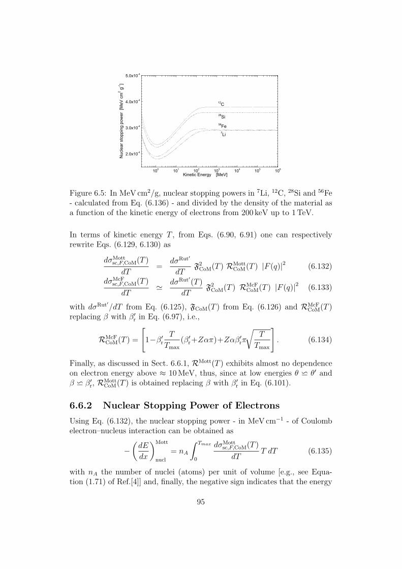
100 101 102 103 104 105 106

2.0x10-4

3.0x10-4

4.0x10-4

5.0x10-4

56Fe7Li

28Si

12C

Nuc

lear

sto

ppin

g po

wer

[M

eV c

m2 g

-1]

Kinetic Energy [MeV]

Figure 6.5: In MeV cm2/g, nuclear stopping powers in 7Li, 12C, 28Si and 56Fe- calculated from Eq. (6.136) - and divided by the density of the material asa function of the kinetic energy of electrons from 200 keV up to 1TeV.

In terms of kinetic energy T , from Eqs. (6.90, 6.91) one can respectivelyrewrite Eqs. (6.129, 6.130) as

dσMottsc,F,CoM(T )

dT=

dσRut′

dTF2CoM(T ) RMott

CoM(T ) |F (q)|2 (6.132)

dσMcFsc,F,CoM(T )

dT≃ dσRut′(T )

dTF2CoM(T ) RMcF

CoM(T ) |F (q)|2 (6.133)

with dσRut′/dT from Eq. (6.125), FCoM(T ) from Eq. (6.126) and RMcFCoM(T )

replacing β with β′r in Eq. (6.97), i.e.,

RMcFCoM(T ) =

[

1−β′r

T

Tmax

(β′r+Zαπ)+Zαβ

′rπ

√

T

Tmax

]

. (6.134)

Finally, as discussed in Sect. 6.6.1, RMott(T ) exhibits almost no dependenceon electron energy above ≈ 10MeV, thus, since at low energies θ ⋍ θ′ andβ ⋍ β′

r, RMottCoM(T ) is obtained replacing β with β′

r in Eq. (6.101).

6.6.2 Nuclear Stopping Power of Electrons

Using Eq. (6.132), the nuclear stopping power - in MeV cm−1 - of Coulombelectron–nucleus interaction can be obtained as

−(

dE

dx

)Mott

nucl

= nA

∫ Tmax

0

dσMottsc,F,CoM(T )

dTT dT (6.135)

with nA the number of nuclei (atoms) per unit of volume [e.g., see Equa-tion (1.71) of Ref.[4]] and, finally, the negative sign indicates that the energy

95

is lost by the electron (thus, achieved by recoil targets). Using the analyticalapproximation derived by McKinley and Feshbach[6], i.e., Eq. (6.133), forthe nuclear stopping power one finds

−(

dE

dx

)McF

nucl

= nA

∫ Tmax

0

dσMcFsc,F,CoM(T )

dTT dT. (6.136)

As already mentioned in Sect. 6.6.1, the large momentum transfers -corresponding to large scattering angles - are disfavored by effects due tothe finite nuclear size accounted for by means of the nuclear form factor(Sect.6.6.1). For instance, the ratios of nuclear stopping powers of electronsin silicon are shown in Ref.[1] as a function of the kinetic energies of electronsfrom 200 keV up to 1TeV. These ratios are the nuclear stopping powerscalculated neglecting i) nuclear size effects (i.e., for |Fexp|2 = 1) and ii) effectsdue to the finite rest mass of the target nucleus [i.e., in Eq. (6.136) replacingdσMcF

sc,F,CoM(T )/dT with dσMcFsc,F (T )/dT from Eq. (6.114)] both divided by that

one obtained using Eq. (6.136). Above a few tens of MeV, a larger stoppingpower is found assuming |Fexp|2 = 1 and, in addition, above a few hundredsof MeV the stopping power largely decreases when the effects of nuclear restmass are not accounted for.

In Fig. 6.5 , the nuclear stopping powers in 7Li, 12C, 28Si and 56Fe areshown as a function of the kinetic energy of electrons from 200 keV up to1TeV. These nuclear stopping powers in MeV cm2/g are calculated fromEq. (6.136) and divided by the density of the medium.

6.6.3 Non-Ionizing Energy-Loss of Electrons

In case of Coulomb scattering of electrons on nuclei, the non-ionizing energy-loss can be calculated using (as discussed in Sect. 6.6.1–6.6.2) the MDCRS orits approximate expression McFDCS [e.g., Eqs. (6.132, 6.133), respectively],once the screened Coulomb fields, finite sizes and rest masses of nuclei areaccounted for, i.e., in Mev/cm

−(

dE

dx

)NIEL

n,Mott

= nA

∫ Tmax

Td

T L(T )dσMott

sc,F,CoM(T )

dTdT (6.137)

or

−(

dE

dx

)NIEL

n,McF

= nA

∫ Tmax

Td

T L(T )dσMcF

sc,F,CoM(T )

dTdT (6.138)

[e.g., see Equation (4.113) at page 402 and, in addition, Sections 4.2.1–4.2.1.2of Ref.[4]], where T is the kinetic energy transferred to the target nucleus,

96

L(T ) is the fraction of T deposited by means of displacement processes. TheLindhard partition function, L(T ), can be approximated using the so-calledNorgett–Robintson–Torrens expression [e.g., see Equations (4.121, 4.123) atpages 404 and 405, respectively, of Ref.[4] (see also references therein)]. Tde =T L(T ) is the so-called damage energy, i.e., the energy deposited by a recoilnucleus with kinetic energy T via displacement damages inside the medium. InEqs. (6.137, 6.138) the integral is computed from the minimum energy Td -the so-called threshold energy for displacement, i.e., that energy necessaryto displace the atom from its lattice position - up to the maximum energyTmax that can be transferred during a single collision process. For instance,Td is about 21 eV in silicon requiring electrons with kinetic energies above≈ 220 kev.

As already discussed with respect to nuclear stopping powers in Sect. 6.6.2,the large momentum transfers (corresponding to large scattering angles) aredisfavored by effects due to the finite nuclear size accounted for by the nu-clear form factor. For instance, the ratios of NIELs for electrons in silicon areshown in Ref.[1] as a function of the kinetic energy of electrons from 220 keVup to 1TeV. These ratios are the NIELs calculated neglecting i) nuclear sizeeffects (i.e., for |Fexp|2 = 1) and ii) effects due to the finite rest mass of the tar-get nucleus [i.e., in Eq. (6.138) replacing dσMcF

sc,F,CoM(T )/dT with dσMcFsc,F (T )/dT

from Eq. (6.114)] both divided by that one obtained using Eq. (6.138). Above≈ 10MeV, the NIEL is ≈ 20% larger assuming |Fexp|2 = 1 and, in addition,above (100–200)MeV the calculated NIEL largely decreases when the effectsof nuclear rest mass are not accounted for.

6.7 G4eSingleScatteringModel

The G4eSingleScatteringModel performs the single scattering interaction ofelectrons on nuclei. The differential cross section (DCS) for the energy trans-ferred is define in the G4ScreeningMottCrossSection class. In this class theM.Boschini’s et al. [7] Mott differential cross Section approximation is im-plemented. This CDS is modified by the introduction of the Moliere’s [10]screening coefficient. In addition the exponential charge distribution NuclearForm Factor is applied [11]. This treatment is fully performed in the center ofmass system and the usual Lorentz transformations are applied to obtainedthe energy and momentum quantities in the laboratory system after scat-tering. This model well simulates the interacting process for low scatteringangles and it is suitable for high energy electrons (from 200 keV) incident onmedium light target nuclei. The nuclear energy loss (i.e. nuclear stoppingpower) is calculated for every single interaction. In addition the production

97

of secondary scattered nuclei is simulated from a threshold kinetic energywhich can be decided by the user (threshold energy for displacement).

6.7.1 The method

In theG4eSingleScatteringModel the method ComputeCrossSectionPerAtom()performs the total cross section computation. The SetupParticle() and theDefineMaterial() methods are called to defined the incident and target par-ticles. Before the total cross section computation, the SetupKinematic()method of the G4ScreeningMottCrossSection class calculates all the physi-cal quantities in the center of mass system (CM). The scattering in the CMsystem is equivalent to the one of an effective particle which interacts witha fixed scattering center. The effective particle rest mass is equal to therelativistic reduced mass of the system µ whose expression is calculated by:

µ = mMc2

Ecm

(6.139)

where m and M are rest masses of the electron and of the target nucleirespectively. Ecm is the total center of mass energy and, since the target isat rest before scattering, its expression is calculated by:

Ecm =√

(mc2)2 + (Mc2)2 + 2E ′Mc2 (6.140)

where E = γ′mc2 is the total energy of the electron before scattering in thelaboratory system. The momentum and the scattering angle of the effectiveparticle are equal to the corresponding quantities calculated in the center ofmass system (p ≡ pcm, θ ≡ θcm) of the incident electron:

pc = p′cMc2

Ecm

(6.141)

where p′ is the momentum of the incident electron calculated in the labora-tory system. The velocity of the effective particle is related with its momen-tum by the following expression:

1

β2= 1 +

(µc2

pc

)2

(6.142)

The integration of the DCS is performed by theNuclearCrossSection() methodof the G4ScreeningMottCrossSection:

σtot = 2π

∫ θmax

θmin

dσ(θ)

dΩsin θdθ (6.143)

98

The integration is performed in the scattering range [0 ;π] but the user candecide to vary the minimum (θmin) and the maximum (θmax) scattering an-gles. The DCS is then given by:

dσ(θ)

dΩ=

(

Ze2

µc2 β2γ

)2RMcF |FN(q)|2

(

2As + 2 sin2(θ/2))2 (6.144)

where Z is the atomic number of the nucleus, As is the screening coefficientwhose expression has been given by Moliere[10] :

As =

(

~

2p aTF

)2[

1.13 + 3.76

(

αZ

β

)2]

(6.145)

where aTF is the Thomas-Fermi screening length given by:

aTF =0.88534 a0

Z1/3(6.146)

and a0 is the Bhor radius. RMcF is the ratio of the Mott to the RutherforDCS given by McKinley and Feshbach approximation [6]:

RMcF =

[

1− β2 sin2(θ/2) + Zαβπ sin(θ/2)(

1− sin(θ/2))

]

(6.147)

The nuclear form factor for the exponential charge distribution is given by[11]:

FN(q) =

[

1 +(qRN)

2

12~2

]−2

(6.148)

where RN is the nuclear radius that is parameterized by:

RN = 1.27A0.27 fm. (6.149)

q is the momentum transferred to the nucleus and it is calculated as:

qc =√

T (T + 2Mc2) (6.150)

where T is the kinetic energy transferred to the nucleus. This kinetic energyis calculated in the GetNewDirection() method as:

T =2Mc2(p′c)2

E2cm

sin2 θ/2. (6.151)

The scattering angle θ calculation is performed in the GetScatteringAngle()method of G4ScreeningMottCrossSection class. By means of AngleDistribu-tion() function the scattering angle is chosen randomly according to the total

99

cross section distribution (p.d.f. probability density function) by means ofthe inverse transform method.

In the SampleSecondary() method of G4eSingleScatteringModel the ki-netic energy of the incident particle after scattering is then calculated asE ′

new = E ′ − T where E ′ is the electron incident kinetic energy (in lab.); inaddition the new particle direction and momentum are obtained from thescattering angle information.


The scattering angle probability density function f(θ) (p.d.f.) is performedby the AngleDistribution() of G4ScreeningMottCrossSection class where theinverse transform method is applied. The normalized cumulative function ofthe cross section is calculated as a function of the scattering angle in thisway:

σn(θ) ≡∫

f(θ)dθ =2π

σtot

∫ θ

0

dσ(t)

dΩsin tdt (6.152)

The normalized cumulative function σn(θ) depends on the DCS and its val-ues range in the interval [0;1]. After this calculation a random number r,uniformly distributed in the same interval [0;1], is chosen in order to fix thecumulative function value (i.e. r ≡ σn(θ)). This number is the probabilityto find the scattering angle in the interval [θ; θ + dθ]. The scattering angleθ is then given by the inverse function of σn(θ).

The threshold energy for displacement Th can by set by the user in her/hisown Physic class by adding the electromagnetic model:G4eSingleCoulombScatteringModel* mod=

new G4eSingleCoulombScatteringModel();

mod->SetRecoilThreshold(Th);

If the energy lost by the incident particle is grater then this threshold valuea new secondary particle is created for transportation processes. The energylost is added to ProposeNonIonizingEnergyDeposit().

NIEL calculation is available in test58.

Bibliography

[1] M. Boschini et al., Nuclear and Non-Ionizing Energy-Loss of Electronswith Low and Relativistic Energies in Materials and Space Environ-

100

ment,Proc. of the ICATPP Conference on Cosmic Rays for Particle andAstroparticle Physics, October 3–7 (2011), Villa Olmo, Como, Italy, S.Giani, C. Leroy, L. Price, P.G. Rancoita and R. Ruchri, Editors, WorldScientific, Singapore (2012); arXiv 1111.4042.

[2] C. Leroy and P.G. Rancoita, Particle Interaction and DisplacementDamage in Silicon Devices operated in Radiation Environments,Rep. Prog. in Phys. 70 (no. 4)(2007), 403–625, doi: 10.1088/0034-4885/70/4/R01.

[3] M. Boschini et al., Nuclear and Non-Ionizing Energy-Loss for CoulombScattered Particles from Low Energy up to Relativistic Regime in SpaceRadiation Environment, Proc. of the ICATPP Conference on Cos-mic Rays for Particle and Astroparticle Physics, October 7–8 (2010),Villa Olmo, Como, Italy, S. Giani, C. Leroy and P.G. Rancoita, Edi-tors, World Scientific, Singapore (2011), 9–23, IBSN: 978-981-4329-02-6;arXiv 1011.4822.

[4] C. Leroy and P.G. Rancoita, Principles of Radiation Interaction in Mat-ter and Detection, 3rd Edition, World Scientific (Singapore) 2011.

[5] T. Lijian, H. Quing and L. Zhengming, Radiat. Phys. Chem. 45 (1995),235–245.

[6] A.J. McKinley and H. Feshbach, Phys. Rev. 74 (1948), 1759–1763.

[7] M. Boschini et al., Rad. Phys. Chem. 90 (2013), 39–66.

[8] E. Zeitler and A. Olsen, Phys. Rev. 136 (1956), A1546-A1552.

[9] H. De Vries, C.W. De Jager, and C. De Vries, Atomic Data and NuclearData Tables 36 (1987), 495.

[10] von G. Moliere, Z. Naturforsh A2 (1947), 133-145; A3 (1948), 78.

[11] A.V. Butkevich et al. Nucl. Instr. and Meth. in Phys. Res. A 488 (2002),282–294.

101

Chapter 7

Energy loss of ChargedParticles

102

7.1 Mean Energy Loss

Energy loss processes are very similar for e + /e− , µ + /µ− and chargedhadrons, so a common description for them was a natural choice in Geant4[1], [2]. Any energy loss process must calculate the continuous and discreteenergy loss in a material. Below a given energy threshold the energy loss iscontinuous and above it the energy loss is simulated by the explicit produc-tion of secondary particles - gammas, electrons, and positrons.

7.1.1 Method

Letdσ(Z,E, T )

dT

be the differential cross-section per atom (atomic number Z) for the ejectionof a secondary particle with kinetic energy T by an incident particle of totalenergy E moving in a material of density ρ. The value of the kinetic energycut-off or production threshold is denoted by Tcut. Below this threshold thesoft secondaries ejected are simulated as continuous energy loss by the inci-dent particle, and above it they are explicitly generated. The mean rate ofenergy loss is given by:

dEsoft(E, Tcut)

dx= nat ·

∫ Tcut

0

dσ(Z,E, T )

dTT dT (7.1)

where nat is the number of atoms per volume in the material. The total crosssection per atom for the ejection of a secondary of energyT > Tcut is

σ(Z,E, Tcut) =

∫ Tmax

Tcut

dσ(Z,E, T )

dTdT (7.2)

where Tmax is the maximum energy transferable to the secondary particle.If there are several processes providing energy loss for a given particle, thenthe total continuous part of the energy loss is the sum:

dEtotsoft(E, Tcut)

dx=∑

i

dEsoft,i(E, Tcut)

dx. (7.3)

These values are pre-calculated during the initialization phase of Geant4

and stored in the dE/dx table. Using this table the ranges of the particlein given materials are calculated and stored in the Range table. The Rangetable is then inverted to provide the InverseRange table. At run time, valuesof the particle’s continuous energy loss and range are obtained using these

103

tables. Concrete processes contributing to the energy loss are not involved inthe calculation at that moment. In contrast, the production of secondarieswith kinetic energies above the production threshold is sampled by eachconcrete energy loss process.

The default energy interval for these tables extends from 100eV to 10TeVand the default number of bins is 77. For muons and for heavy particles en-ergy loss processes models are valid for higher energies and can be extended.For muons uppper limit may be set to 1000PeV .

7.1.2 General Interfaces

There are a number of similar functions for discrete electromagnetic pro-cesses and for electromagnetic (EM) packages an additional base classes weredesigned to provide common computations [2]. Common calculations for dis-crete EM processes are performed in the class G4V EnergyLossProcess. De-rived classes (7.1) are concrete processes providing initialisation. The physicsmodels are implemented using the G4V EmModel interface. Each processmay have one or many models defined to be active over a given energy rangeand set of G4Regions. Models are implementing computation of energy loss,cross section and sampling of final state. The list of EM processes and modelsfor gamma incident is shown in Table 7.1.

7.1.3 Step-size Limit

Continuous energy loss imposes a limit on the step-size because of the energydependence of the cross sections. It is generally assumed in MC programs(for example, Geant3) that the cross sections are approximately constantalong a step, i.e. the step size should be small enough, so that the changein cross section along the step is also small. In principle one must use verysmall steps in order to insure an accurate simulation, however the computingtime increases as the step-size decreases.

For EM processes the exact solution is available (see 7.3) but is is notimplemented yet for all physics processes including hadronics. A good com-promise is to limit the step-size by not allowing the stopping range of theparticle to decrease by more than ∼ 20 % during the step. This conditionworks well for particles with kinetic energies > 1 MeV, but for lower energiesit gives too short step-sizes, so must be relaxed. To solve this problem alower limit on the step-size was introduced. A smooth StepFunction, with2 parameters, controls the step size. At high energy the maximum stepsize is defined by Step/Range ∼ αR (parameter dRoverRange). By defaultαR = 0.2. As the particle travels the maximum step size decreases gradually

104

Table 7.1: List of process and model classes for charged particles.

EM process EM model Ref.G4eIonisation G4MollerBhabhaModel 8.1

G4LivermoreIonisationModel 9.9G4PenelopeIonisationModel 10.1.7G4PAIModel 7.5G4PAIPhotModel 7.5

G4ePolarizedIonisation G4PolarizedMollerBhabhaModel 17.1G4MuIonisation G4MuBetheBlochModel 13.1

G4PAIModel 7.5G4PAIPhotModel 7.5

G4hIonisation G4BetheBlochModel 12.1G4BraggModel 12.1G4ICRU73QOModel 12.2.1G4PAIModel 7.5G4PAIPhotModel 7.5

G4ionIonisation G4BetheBlochModel 12.1G4BetheBlochIonGasModel 12.1G4BraggIonModel 12.1G4BraggIonGasModel 12.1G4IonParametrisedLossModel 12.2.4

G4NuclearStopping G4ICRU49NuclearStoppingModel 12.1.3G4mplIonisation G4mplIonisationWithDeltaModelG4eBremsstrahlung G4SeltzerBergerModel 8.2.1

G4eBremsstrahlungRelModel 8.2.2G4LivermoreBremsstrahlungModel 9.10G4PenelopeBremsstrahlungModel 10.1.6

G4ePolarizedBremsstrahlung G4PolarizedBremsstrahlungModel 17.1G4MuBremsstrahlung G4MuBremsstrahlungModel 13.2G4hBremsstrahlung G4hBremsstrahlungModelG4MuPairProduction G4MuPairProductionModel 13.3G4hPairProduction G4hPairProductionModel

105

until the range becomes lower than ρR (parameter finalRange). Default final-Range ρR = 1mm. For the case of a particle range R > ρR the StepFunctionprovides limit for the step size ∆Slim by the following formula:

∆Slim = αRR + ρR(1− αR)(

2− ρRR

)

. (7.4)

In the opposite case of a small range ∆Slim = R. The figure below shows theratio step/range as a function of range if step limitation is determined onlyby the expression (7.4).

step−−−−−−range

range

finalRange

1

dRoverRange

The parameters of StepFunction can be overwritten using an UI command:

/process/eLoss/StepFunction 0.2 1 mmTo provide more accurate simulation of particle ranges in physics constructorsG4EmStandardPhysics option3 andG4EmStandardPhysics option4more strictstep limitation is chosen for different particle types.

7.1.4 Run Time Energy Loss Computation

The computation of the mean energy loss after a given step is done by usingthe dE/dx, Range, and InverseRange tables. The dE/dx table is used ifthe energy deposition (∆T ) is less than allowed limit ∆T < ξT0, where ξ is

106

linearLossLimit parameter (by default ξ = 0.01), T0 is the kinetic energyof the particle. In that case

∆T =dE

dx∆s, (7.5)

where ∆T is the energy loss, ∆s is the true step length. When a largerpercentage of energy is lost, the mean loss can be written as

∆T = T0 − fT (r0 −∆s) (7.6)

where r0 the range at the beginning of the step, the function fT (r) is theinverse of the Range table (i.e. it gives the kinetic energy of the particle fora range value of r). By default spline approximation is used to retrieve avalue from dE/dx, Range, and InverseRange tables. The spline flag can bechanged using an UI command:

/process/em/spline falseAfter the mean energy loss has been calculated, the process computes theactual energy loss, i.e. the loss with fluctuations. The fluctuation models aredescribed in Section 7.2.

If deexcitation module (see 14.1) is enabled then simulation of atomic de-excitation is performed using information on step length and ionisation crosssection. Fluorescence gamma and Auger electrons are produced above thesame threshold energy as δ-electrons and bremsstrahlung gammas. FollowingUI commands can be used to enable atomic relaxation:/process/em/deexcitation myregion true true true/process/em/fluo true/process/em/auger true/process/em/pixe true/process/em/deexcitationIgnoreCut true

The last command means that production threshold for electrons and gam-mas are not checked, so full atomic de-excitation decay chain is simulated.

7.1.5 Energy Loss by Heavy Charged Particles

To save memory in the case of positively charged hadrons and ions energyloss, dE/dx, Range and InverseRange tables are constructed only for pro-ton, antiproton, muons, pions, kaons, and Generic Ion. The energy loss forother particles is computed from these tables at the scaled kinetic energyTscaled :

Tscaled = TMbase

Mparticle

, (7.7)

107

where T is the kinetic energy of the particle,Mbase andMparticle are the massesof the base particle (proton or kaon) and particle. For positively changedhadrons with non-zero spin proton is used as a based particle, for negativelycharged hadrons with non-zero spin - antiproton, for charged particles withzero spin - K+ or K− correspondingly. The virtual particle Generic Ion isused as a base particle for for all ions with Z > 2. It has mass, change andother quantum numbers of the proton. The energy loss can be defined viascaling relation:

dE

dx(T ) = q2eff (F1(T )

dE

dx base(Tscaled) + F2(T, qeff )), (7.8)

where qeff is particle effective change in units of positron charge, F1 andF2 are correction function taking into account Birks effect, Block correction,low-energy corrections based on data from evaluated data bases [5]. For ahadron qeff is equal to the hadron charge, for a slow ion effective charge isdifferent from the charge of the ion’s nucleus, because of electron exchangebetween transporting ion and the media. The effective charge approach isused to describe this effect [3]. The scaling relation (7.7) is valid for anycombination of two heavy charged particles with accuracy corresponding tohigh order mass, charge and spin corrections [4].

Bibliography

[1] S. Agostinelli et al., Geant4 – a simulation toolkit Nucl. Instr. Meth.A506 (2003) 250.


[3] J.F. Ziegler and J.M. Manoyan, Nucl. Instr. and Meth. B35 (1988) 215.

[4] ICRU (A. Allisy et al), Stopping Powers and Ranges for Protons andAlpha Particles, ICRU Report 49, 1993.

[5] ICRU (R. Bimbot et al), Stopping of Ions Heavier than Helium, Journalof the ICRU Vol5 No1 (2005) Report 73.

108

7.2 Energy Loss Fluctuations

The total continuous energy loss of charged particles is a stochastic quan-tity with a distribution described in terms of a straggling function. Thestraggling is partially taken into account in the simulation of energy lossby the production of δ-electrons with energy T > Tcut (Eq.7.2). However,continuous energy loss (Eq.7.1) also has fluctuations. Hence in the currentGEANT4 implementation different models of fluctuations implementing theG4V EmFluctuationModel interface:

• G4BohrFluctuations;

• G4IonFluctuations;

• G4PAIModel;

• G4PAIPhotModel;

• G4UniversalFluctuation.

The last model is the default one used in main Physics List and will be de-scribed below. Other models have limited applicability and will be describedin chapters for ion ionisation and PAI models.

7.2.1 Fluctuations in Thick Absorbers

The total continuous energy loss of charged particles is a stochastic quantitywith a distribution described in terms of a straggling function. The strag-gling is partially taken into account in the simulation of energy loss by theproduction of δ-electrons with energy T > Tc. However, continuous energyloss also has fluctuations. Hence in the current GEANT4 implementationtwo different models of fluctuations are applied depending on the value ofthe parameter κ which is the lower limit of the number of interactions of theparticle in a step. The default value chosen is κ = 10. In the case of a highrange cut (i.e. energy loss without delta ray production) for thick absorbersthe following condition should be fulfilled:

∆E > κ Tmax (7.9)

where ∆E is the mean continuous energy loss in a track segment of length s,and Tmax is the maximum kinetic energy that can be transferred to the atomicelectron. If this condition holds the fluctuation of the total (unrestricted)energy loss follows a Gaussian distribution. It is worth noting that this

109

condition can be true only for heavy particles, because for electrons, Tmax =T/2, and for positrons, Tmax = T , where T is the kinetic energy of theparticle. In order to simulate the fluctuation of the continuous (restricted)energy loss, the condition should be modified. After a study, the followingconditions have been chosen:

∆E > κ Tc (7.10)

Tmax <= 2 Tc (7.11)

where Tc is the cut kinetic energy of δ-electrons. For thick absorbers thestraggling function approaches the Gaussian distribution with Bohr’s vari-ance [4]:

Ω2 = 2πr2emec2Nel

Z2h

β2Tcs

(

1− β2

2

)

, (7.12)

where re is the classical electron radius, Nel is the electron density of themedium, Zh is the charge of the incident particle in units of positron charge,and β is the relativistic velocity.

7.2.2 Fluctuations in Thin Absorbers

If the conditions 7.10 and 7.11 are not satisfied the model of energy fluctua-tions in thin absorbers is applied. The formulas used to compute the energyloss fluctuation (straggling) are based on a very simple physics model of theatom. It is assumed that the atoms have only two energy levels with bindingenergies E1 and E2. The particle-atom interaction can be an excitation withenergy loss E1 or E2, or ionisation with energy loss distributed according toa function g(E) ∼ 1/E2 :

∫ Tup

E0

g(E) dE = 1 =⇒ g(E) =E0TupTup − E0

1

E2. (7.13)

The macroscopic cross section for excitation (i = 1, 2) is

Σi = CfiEi

ln[2mc2 (βγ)2/Ei]− β2

ln[2mc2 (βγ)2/I]− β2(1− r) (7.14)

and the ionisation cross section is

Σ3 = CTup − E0

E0Tup ln(Tup

E0)r (7.15)

where E0 denotes the ionisation energy of the atom, I is the mean ionisationenergy, Tup is the production threshold for delta ray production (or the max-imum energy transfer if this value smaller than the production threshold),

110

Ei and fi are the energy levels and corresponding oscillator strengths of theatom, and C and r are model parameters.

The oscillator strengths fi and energy levels Ei should satisfy the con-straints

f1 + f2 = 1 (7.16)

f1· lnE1 + f2· lnE2 = lnI. (7.17)

The cross section formulas 7.14,7.15 and the sum rule equations 7.16,7.17can be found e.g. in Ref. [1]. The model parameter C can be defined in thefollowing way. The numbers of collisions (ni, i = 1, 2 for excitation and 3 forionisation) follow the Poisson distribution with a mean value 〈ni〉. In a stepof length ∆x the mean number of collisions is given by

〈ni〉 = ∆x Σi (7.18)

The mean energy loss in a step is the sum of the excitation and ionisationcontributions and can be written as

dE

dx·∆x =

Σ1E1 + Σ2E2 +

∫ Tup

E0

Eg(E)dE

∆x. (7.19)

From this, using Eq. 7.14 - 7.17, one can see that

C = dE/dx. (7.20)

The other parameters in the fluctuation model have been chosen in the follow-ing way. Z· f1 and Z· f2 represent in the model the number of loosely/tightlybound electrons

f2 = 0 for Z = 1 (7.21)

f2 = 2/Z for Z ≥ 2 (7.22)

E2 = 10 eV Z2 (7.23)

E0 = 10 eV . (7.24)

Using these parameter values, E2 corresponds approximately to the K-shellenergy of the atoms ( and Zf2 = 2 is the number of K-shell electrons).The parameters f1 and E1 can be obtained from Eqs. 7.16 and 7.17. Theparameter r is the only variable in the model which can be tuned. Thisparameter determines the relative contribution of ionisation and excitation tothe energy loss. Based on comparisons of simulated energy loss distributionsto experimental data, its value has been fixed as

r = 0.55 (7.25)

111

7.2.3 Width Correction Algorithm

This simple parametrization and sampling in the model give good values forthe most probable energy loss in thin layers. The width of the energy lossdistribution (Full Width at Half Maximum, FWHM) in most of the casesis too small. In order to get good FWHM values a relatively simple widthcorrection algorithm has been applied. This algorithm rescales the energylevels E1, E2 and the number of excitations n1, n2 in such a way that themean energy loss remains the same. Using this width correction scheme themodel gives not only good most probable energy loss, but good FWHM valuetoo.

Width correction algorithm is in the model since version 9.2. The updatedversion in the model (in version 9.4) causes an important change in thebehaviour of the model: the results become much more stable, i.e. the resultsdo not change practically when the cuts and/or the stepsizes are changing.Another important change: the (unphysical) second peak or shoulder in theenergy loss distribution which can be seen in some cases (energy loss in thingas layers) in older versions of the model disappeared. Limit of validityof the model for thin targets: the model gives good (reliable) energy lossdistribution if the mean energy loss in the target is ≥ (few times) ∗ Iexc,where Iexc is the mean excitation energy of the target material.

This simple model of energy loss fluctuations is rather fast and can beused for any thickness of material. This has been verified by performingmany simulations and comparing the results with experimental data, such asthose in Ref.[2]. As the limit of validity of Landau’s theory is approached,the loss distribution approaches the Landau form smoothly.

7.2.4 Sampling of Energy Loss

If the mean energy loss and step are in the range of validity of the Gaussianapproximation of the fluctuation (7.10 and 7.11), the Gaussian sampling isused to compute the actual energy loss (7.12). For smaller steps the energyloss is computed in the model under the assumption that the step length (orrelative energy loss) is small and, in consequence, the cross section can beconsidered constant along the step. The loss due to the excitation is

∆Eexc = n1E1 + n2E2 (7.26)

where n1 and n2 are sampled from a Poisson distribution. The energy lossdue to ionisation can be generated from the distribution g(E) by the inverse

112

transformation method :

u = F (E) =

∫ E

E0

g(x)dx (7.27)

E = F−1(u) =E0

1− uTup−E0

Tup

(7.28)

where u is a uniformly distributed random number ∈ [0, 1]. The contributioncoming from the ionisation will then be

∆Eion =n3∑

j=1

E0

1− ujTup−E0

Tup

(7.29)

where n3 is the number of ionisations sampled from the Poisson distribution.The total energy loss in a step will be ∆E = ∆Eexc +∆Eion and the energyloss fluctuation comes from fluctuations in the number of collisions ni andfrom the sampling of the ionisation loss.

Bibliography

[1] H. Bichsel Rev.Mod.Phys. 60 (1988) 663.

[2] K. Lassila-Perini, L. Urban Nucl.Inst.Meth. A362(1995) 416.

[3] geant3 manual Cern Program Library Long Writeup W5013 (1994)

[4] ICRU (A. Allisy et al), Stopping Powers and Ranges for Protons andAlpha Particles, ICRU Report 49 (1993).

113

7.3 Correcting the Cross Section for Energy

Variation

As described in Sections 7.1 and 3.1.2 the step size limitation is providedby energy loss processes in order to insure the precise calculation of theprobability of particle interaction. It is generally assumed in Monte Carloprograms that the particle cross sections are approximately constant during astep, hence the reaction probability p at the end of the step can be expressedas

p = 1− exp (−nsσ(Ei)) , (7.30)

where n is the density of atoms in the medium, s is the step length, Ei is theenergy of the incident particle at the beginning of the step, and σ(Ei) is thereaction cross section at the beginning of the step.

However, it is possible to sample the reaction probability from the exactexpression

p = 1− exp

(

−∫ Ef

Ei

nσ(E)ds

)

, (7.31)

where Ef is the energy of the incident particle at the end of the step, by usingthe integral approach to particle transport. This approach is available for pro-cesses implemented via the G4V EnergyLossProcess and G4V EmProcessinterfaces.

The Monte Carlo method of integration is used for sampling the reactionprobability [1]. It is assumed that during the step the reaction cross sectionsmaller, than some value σ(E) < σm. The mean free path for the given stepis computed using σm. If the process is chosen as the process happens at thestep, the sampling of the final state is performed only with the probability p =σ(Ef )/σm, alternatively no interaction happen and tracking of the particleis continued. To estimate the maximum value σm for the given tracking stepat Geant4 initialisation the energy Em of absoluted maximum σmax of thecross section for given material is determined and stored. If at the trackingtime particle energy E < Em, then σm = σ(E). For higher initial energiesif ξE > Em then σm = min(σ(E), σ(ξE)). In the opposit case σm = σmax.Here ξ is a parameter of the algorithm. Its optimal value is connected withthe value of the dRoverRange parameter (see sub-chapter 7.1), by defaultξ = 1−αR = 0.8. Note, that described method is precise if the cross sectionhas only one maximum, which is a typical case for electromagnetic processes.

The integral variant of step limitation is the default for theG4eIonisation,G4eBremsstrahlung and some otehr process but is not automatically acti-vated for others. To do so the boolean UI command can be used:

114

/process/eLoss/integral true

The integral variant of the energy loss sampling process is less dependenton values of the production cuts [2] and allows to have less step limitation,however it should be applied on a case-by-case basis because may requireextra CPU.

Bibliography

[1] V.N.Ivanchenko et al., Proc. of Int. Conf. MC91: Detector and eventsimulation in high energy physics, Amsterdam 1991, pp. 79-85. (HEPINDEX 30 (1992) No. 3237).


115

7.4 Conversion from Cut in Range to Energy

Threshold

In Geant4 charged particles are tracked to the end of their range. The dif-ferential cross section of δ-electron productions and bremsstrahlung growrapidly when secondary energy decrease. If all secondary particles will betracked the CPU performance of any Monte Carlo code will be pure. Thetraditional solution is to use cuts. The specific of Geant4 [1] is that userprovides value of cut in term of cut in range, which is unique for definedG4Region or for the complete geometry [2].

Range is used, rather than energy, as a more natural concept for designinga coherent policy for different particles and materials. Definition of the cer-tain value of the cut in range means the requirement for precision of spatialradioactive dose deposition. This conception is more strict for a simulationcode and provides less handles for user to modify final results. At the sametime, it ensures that simulation validated in one geometry is valid also forthe other geometries.

The value of cut is defined for electrons, positrons, gamma and protons.At the beginning of initialization of Geant4 physics the conversion is per-formed from unique cut in range to cuts (production thresholds) in kineticenergy for each G4MaterialCutsCouple [2]. At that moment no energy lossor range table is created, so computation should be performed using originalformulas. For electrons and positrons ionization above 10keV a simplifiedBerger-Seltzer energy loss formula (8.2) is used, in which the density correc-tion term is omitted. The contribution of the bremsstrahlung is added usingempirical parameterized formula. For T < 10keV the linear dependence ofionization losses on electron velocity is assumed, bremsstrahlung contributionis neglected. The stopping range is defined as

R(T ) =

∫ T

0

1

(dE/dx)dE. (7.32)

The integration has been done analytically for the low energy part and numer-ically above an energy limit 1 keV . For each cut in range the correspondingkinetic energy can be found out. If obtained production threshold in kineticenergy cannot be below the parameter lowlimit (default 1 keV ) and abovehighlimit (default 10 GeV ). If in specific application lower threshold is re-quired, then the allowed energy cut needs to be extended:

G4ProductionCutsTable::GetProductionCutsTable()→SetEnergyRange(lowlimit,highlimit);

or via UI commands

116

/cuts/setMinCutEnergy 100 eV/cuts/setMaxCutEnergy 100 TeV

In contrary to electrons, gammas has no range, so some approximation shouldbe used for range to energy conversion. An approximate empirical formula isused to compute the absorption cross section of a photon in an element σabs.Here, the absorption cross section means the sum of the cross sections ofthe gamma conversion, Compton scattering and photoelectric effect. Theseprocesses are the “destructive” processes for photons: they destroy the pho-ton or decrease its energy. The coherent or Rayleigh scattering changes thedirection of the gamma only; its cross section is not included in the absorp-tion cross section. The AbsorptionLength Labs vector is calculated for everymaterial as

Labs = 5/σabs. (7.33)

The factor 5 comes from the requirement that the probability of having no’destructive’ interaction should be small, hence

exp(−Labsσabs) = exp(−5) = 6.7× 10−3. (7.34)

The photon cross section for a material has a minimum at a certain energyEmin. Correspondingly Labs has a maximum at E = Emin, the value of themaximal Labs is the biggest ”meaningful” cut in absorption length. If the cutgiven by the user is bigger than this maximum, a warning is printed and thecut in kinetic energy is set to the highlimit.

The cut for proton is introduced with Geant4 v9.3. The main goal ofthis cut is to limit production of all recoil ions including protons in elasticscattering processes. A simple linear conversion formula is used to computeenergy threshold from the value of cut in range, in particular, the cut inrange 1 mm corresponds to the production threshold 100keV .

The conversion from range to energy can be studied usingG4EmCalculatorclass. This class allows access or recalculation of energy loss, ranges and othervalues. It can be instantiated and at any place of user code and can be usedafter initialisation of Physics Lists:

G4EmCalculator calc;calc.ComputeEnergyCutFromRangeCut(range, particle, material);

here particle and material may be string names or corresponding const point-ers to G4ParticleDefinition and G4Material.

117

Bibliography

[1] Geant4 Collaboration (S. Agostinelli et al.), Nucl. Instr. Meth. A506(2003) 250.

[2] J. Allison et al., IEEE Trans. Nucl. Sci., 53 (2006) 270.

118

7.5 Photoabsorption Ionization Model

7.5.1 Cross Section for Ionizing Collisions

The Photoabsorption Ionization (PAI) model describes the ionization energyloss of a relativistic charged particle in matter. For such a particle, thedifferential cross section dσi/dω for ionizing collisions with energy transfer ωcan be expressed most generally by the following equations [1]:

dσidω

=2πZe4

mv2

f(ω)

ω |ε(ω)|2[

ln2mv2

ω |1− β2ε|−

−ε1 − β2 |ε|2ε2

arg(1− β2ε∗)

]

+F (ω)

ω2

, (7.35)

F (ω) =

∫ ω

0

f(ω′)

|ε(ω′)|2dω′,

f(ω) =mωε2(ω)

2π2ZN~2.

Here m and e are the electron mass and charge, ~ is Planck’s constant,β = v/c is the ratio of the particle’s velocity v to the speed of light c, Zis the effective atomic number, N is the number of atoms (or molecules)per unit volume, and ε = ε1 + iε2 is the complex dielectric constant of themedium. In an isotropic non-magnetic medium the dielectric constant canbe expressed in terms of a complex index of refraction, n(ω) = n1 + in2,ε(ω) = n2(ω). In the energy range above the first ionization potential I1for all cases of practical interest, and in particular for all gases, n1 ∼ 1.Therefore the imaginary part of the dielectric constant can be expressed interms of the photoabsorption cross section σγ(ω):

ε2(ω) = 2n1n2 ∼ 2n2 =N~c

ωσγ(ω).

The real part of the dielectric constant is calculated in turn from the disper-sion relation

ε1(ω)− 1 =2N~c

πV.p.

∫ ∞

0

σγ(ω′)

ω′2 − ω2dω′,

where the integral of the pole expression is considered in terms of the princi-pal value. In practice it is convenient to calculate the contribution from thecontinuous part of the spectrum only. In this case the normalized photoab-sorption cross section

119

σγ(ω) =2π2

~e2Z

mcσγ(ω)

[∫ ωmax

I1

σγ(ω′)dω′

]−1

, ωmax ∼ 100 keV

is used, which satisfies the quantum mechanical sum rule [2]:

∫ ωmax

I1

σγ(ω′)dω′ =

2π2~e2Z

mc.

The differential cross section for ionizing collisions is expressed by the pho-toabsorption cross section in the continuous spectrum region:

dσidω

=α

πβ2

σγ(ω)

ω |ε(ω)|2[

ln2mv2

ω |1− β2ε|−

−ε1 − β2 |ε|2ε2

arg(1− β2ε∗)

]

+1

ω2

∫ ω

I1

σγ(ω′)

|ε(ω′)|2dω′

, (7.36)

ε2(ω) =N~c

ωσγ(ω),

ε1(ω)− 1 =2N~c

πV.p.

∫ ωmax

I1

σγ(ω′)

ω′2 − ω2dω′.

For practical calculations using Eq. 7.35 it is convenient to represent thephotoabsorption cross section as a polynomial in ω−1 as was proposed in [3]:

σγ(ω) =4∑

k=1

a(i)k ω

−k,

where the coefficients, a(i)k result from a separate least-squares fit to experi-

mental data in each energy interval i. As a rule the interval borders are equalto the corresponding photoabsorption edges. The dielectric constant can nowbe calculated analytically with elementary functions for all ω, except nearthe photoabsorption edges where there are breaks in the photoabsorptioncross section and the integral for the real part is not defined in the sense ofthe principal value.

The third term in Eq. (7.35), which can only be integrated numerically,results in a complex calculation of dσi/dω. However, this term is dominant

120

for energy transfers ω > 10 keV , where the function |ε(ω)|2 ∼ 1. This is clearfrom physical reasons, because the third term represents the Rutherford crosssection on atomic electrons which can be considered as quasifree for a givenenergy transfer [4]. In addition, for high energy transfers, ε(ω) = 1−ω2

p/ω2 ∼

1, where ωp is the plasma energy of the material. Therefore the factor |ε(ω)|−2

can be removed from under the integral and the differential cross section ofionizing collisions can be expressed as:

dσidω

=α

πβ2 |ε(ω)|2

σγ(ω)

ω

[

ln2mv2

ω |1− β2ε|−

−ε1 − β2 |ε|2ε2

arg(1− β2ε∗)

]

+1

ω2

∫ ω

I1

σγ(ω′)dω′

. (7.37)

This is especially simple in gases when |ε(ω)|−2 ∼ 1 for all ω > I1 [4].

7.5.2 Energy Loss Simulation

For a given track length the number of ionizing collisions is simulated by aPoisson distribution whose mean is proportional to the total cross section ofionizing collisions:

σi =

∫ ωmax

I1

dσ(ω′)

dω′ dω′.

The energy transfer in each collision is simulated according to a distributionproportional to

σi(> ω) =

∫ ωmax

ω

dσ(ω′)

dω′ dω′.

The sum of the energy transfers is equal to the energy loss. PAI ionisation isimplemented according to the model approach (class G4PAIModel) allowinga user to select specific models in different regions. Here is an example physicslist:

const G4RegionStore* theRegionStore = G4RegionStore::GetInstance();

G4Region* gas = theRegionStore->GetRegion("VertexDetector");

...

if (particleName == "e-")

...

G4eIonisation* eion = new G4eIonisation();

121

G4PAIModel* pai = new G4PAIModel(particle,"PAIModel");

// here 0 is the highest priority in region ’gas’

eion->AddEmModel(0,pai,pai,gas);

...

...

It shows how to select the G4PAIModel to be the preferred ionisation modelfor electrons in a G4Region named VertexDetector. The first argument inAddEmModel is 0 which means highest priority.

The class G4PAIPhotonModel generates both δ-electrons and photons assecondaries and can be used for more detailed descriptions of ionisation spacedistribution around the particle trajectory.

7.5.3 Photoabsorption Cross Section at Low Energies

The photoabsorption cross section, σγ(ω), where ω is the photon energy, isused in Geant4 for the description of the photo-electric effect, X-ray trans-portation and ionization effects in very thin absorbers. As mentioned in thediscussion of photoabsorption ionization (see section 7.5), it is convenient torepresent the cross section as a polynomial in ω−1 [5] :

σγ(ω) =4∑

k=1

a(i)k ω

−k. (7.38)

Using cross sections from the original Sandia data tables, calculations of pri-mary ionization and energy loss distributions produced by relativistic chargedparticles in gaseous detectors show clear disagreement with experimentaldata, especially for gas mixtures which include xenon.

Therefore a special investigation was performed [6] by fitting the coefficients

a(i)k to modern data from synchrotron radiation experiments in the energy

range of 10 − 50 eV . The fits were performed for elements typically usedin detector gas mixtures: hydrogen, fluorine, carbon, nitrogen and oxygen.Parameters for these elements were extracted from data on molecular gasessuch as N2, O2, CO2, CH4, and CF4 [7, 8]. Parameters for the noble gaseswere found using data given in the tables [9, 10].

122

7.5.4 Status of this document

01.12.05 expanded discussion by V. Grichine08.05.02 re-written by D.H. Wright16.11.98 created by V. Grichine20.11.12 updated by V. Ivanchenko

Bibliography

[1] Asoskov V.S., Chechin V.A., Grichine V.M. at el, Lebedev Instituteannual report, v. 140, p. 3 (1982)

[2] Fano U., and Cooper J.W. Rev.Mod.Phys., v. 40, p. 441 (1968)


[4] AllisonW.W.M., and Cobb J. Ann.Rev.Nucl.Part.Sci., v.30,p.253 (1980)


[6] Grichine V.M., Kostin A.P., Kotelnikov S.K. et al., Bulletin of the Lebe-dev Institute no. 2-3, 34 (1994).

[7] Lee L.C. et al., J.Q.S.R.T., v. 13, p. 1023 (1973).

[8] Lee L.C. et al., Journ. of Chem. Phys., v. 67, p. 1237 (1977).

[9] G.V. Marr and J.B. West, Atom. Data Nucl. Data Tabl., v. 18, p. 497(1976).

[10] J.B. West and J. Morton, Atom. Data Nucl. Data Tabl., v. 30, p. 253(1980).

123

Chapter 8

Electron and Positron Incident

124

8.1 Ionization

8.1.1 Method

The G4eIonisation class provides the continuous and discrete energy lossesof electrons and positrons due to ionization in a material according to theapproach described in Section 7.1. The value of the maximum energy trans-ferable to a free electron Tmax is given by the following relation:

Tmax =

E −mc2 for e+

(E −mc2)/2 for e−(8.1)

where mc2 is the electron mass. Above a given threshold energy the energyloss is simulated by the explicit production of delta rays by Moller scattering(e−e−), or Bhabha scattering (e+e−). Below the threshold the soft electronsejected are simulated as continuous energy loss by the incident e±.

8.1.2 Continuous Energy Loss

The integration of 7.1 leads to the Berger-Seltzer formula [1]:

dE

dx

]

T<Tcut

= 2πr2emc2nel

1

β2

[

ln2(γ + 1)

(I/mc2)2+ F±(τ, τup)− δ

]

(8.2)

withre classical electron radius: e2/(4πǫ0mc

2)mc2 mass energy of the electronnel electron density in the materialI mean excitation energy in the materialγ E/mc2

β2 1− (1/γ2)τ γ − 1Tcut minimum energy cut for δ -ray productionτc Tcut/mc

2

τmax maximum energy transfer: τ for e+, τ/2 for e−

τup min(τc, τmax)δ density effect function.

In an elemental material the electron density is

nel = Z nat = ZNavρ

A.

125

Nav is Avogadro’s number, ρ is the material density, and A is the mass of amole. In a compound material

nel =∑

i

Zi nati =∑

i

ZiNavwiρ

Ai

,

where wi is the proportion by mass of the ith element, with molar mass Ai .The mean excitation energies I for all elements are taken from [2].The functions F± are given by :

F+(τ, τup) = ln(ττup) (8.3)

−τ2up

τ

[

τ + 2τup −3τ 2upy

2−(

τup −τ 3up3

)

y2 −(

τ 2up2

− ττ 3up3

+τ 4up4

)

y3]

F−(τ, τup) = −1− β2 (8.4)

+ ln [(τ − τup)τup] +τ

τ − τup+

1

γ2

[

τ 2up2

+ (2τ + 1) ln(

1− τupτ

)

]

where y = 1/(γ + 1).The density effect correction is calculated according to the formalism of

Sternheimer [3]:x is a kinetic variable of the particle : x = log10(γβ) = ln(γ2β2)/4.606,and δ(x) is defined by

for x < x0 : δ(x) = 0for x ∈ [x0, x1] : δ(x) = 4.606x− C + a(x1 − x)m

for x > x1 : δ(x) = 4.606x− C(8.5)

where the matter-dependent constants are calculated as follows:

hνp = plasma energy of the medium =√

4πnelr3emc2/α =

√4πnelre~c

C = 1 + 2 ln(I/hνp)xa = C/4.606a = 4.606(xa − x0)/(x1 − x0)

m

m = 3.(8.6)

For condensed media

I < 100 eV

for C ≤ 3.681 x0 = 0.2 x1 = 2for C > 3.681 x0 = 0.326C − 1.0 x1 = 2

I ≥ 100 eV

for C ≤ 5.215 x0 = 0.2 x1 = 3for C > 5.215 x0 = 0.326C − 1.5 x1 = 3

126

and for gaseous media

for C < 10. x0 = 1.6 x1 = 4for C ∈ [10.0, 10.5[ x0 = 1.7 x1 = 4for C ∈ [10.5, 11.0[ x0 = 1.8 x1 = 4for C ∈ [11.0, 11.5[ x0 = 1.9 x1 = 4for C ∈ [11.5, 12.25[ x0 = 2. x1 = 4for C ∈ [12.25, 13.804[ x0 = 2. x1 = 5for C ≥ 13.804 x0 = 0.326C − 2.5 x1 = 5.

8.1.3 Total Cross Section per Atom and Mean FreePath

The total cross section per atom for Moller scattering (e−e−) and Bhabhascattering (e+e−) is obtained by integrating Eq. 7.2. In Geant4 Tcut isalways 1 keV or larger. For delta ray energies much larger than the excitationenergy of the material (T ≫ I), the total cross section becomes [1] for Mollerscattering,

σ(Z,E, Tcut) =2πr2eZ

β2(γ − 1)× (8.7)

[

(γ − 1)2

γ2

(

1

2− x

)

+1

x− 1

1− x− 2γ − 1

γ2ln

1− x

x

]

,

and for Bhabha scattering (e+e−),

σ(Z,E, Tcut) =2πr2eZ

(γ − 1)× (8.8)

[

1

β2

(

1

x− 1

)

+ B1 ln x+ B2(1− x)− B3

2(1− x2) +

B4

3(1− x3)

]

.

Hereγ = E/mc2 B1 = 2− y2

β2 = 1− (1/γ2) B2 = (1− 2y)(3 + y2)x = Tcut/(E −mc2) B3 = (1− 2y)2 + (1− 2y)3

y = 1/(γ + 1) B4 = (1− 2y)3.

The above formulas give the total cross section for scattering above thethreshold energies

T thrMoller = 2Tcut and T thr

Bhabha = Tcut. (8.9)

In a given material the mean free path is then

λ = (nat · σ)−1 or λ = (∑

i nati · σi)−1 . (8.10)

127

8.1.4 Simulation of Delta-ray Production

Differential Cross Section

For T ≫ I the differential cross section per atom becomes [1] for Mollerscattering,

dσ

dǫ=

2πr2eZ

β2(γ − 1)× (8.11)

[

(γ − 1)2

γ2+

1

ǫ

(

1

ǫ− 2γ − 1

γ2

)

+1

1− ǫ

(

1

1− ǫ− 2γ − 1

γ2

)]

and for Bhabha scattering,

dσ

dǫ=

2πr2eZ

(γ − 1)

[

1

β2ǫ2− B1

ǫ+ B2 −B3ǫ+ B4ǫ

2

]

. (8.12)

Here ǫ = T/(E −mc2). The kinematical limits of ǫ are

ǫ0 =Tcut

E −mc2≤ ǫ ≤ 1

2for e−e− ǫ0 =

TcutE −mc2

≤ ǫ ≤ 1 for e+e−.

Sampling

The delta ray energy is sampled according to methods discussed in Chapter2. Apart from normalization, the cross section can be factorized as

dσ

dǫ= f(ǫ)g(ǫ). (8.13)

For e−e− scattering

f(ǫ) =1

ǫ2ǫ0

1− 2ǫ0(8.14)

g(ǫ) =4

9γ2 − 10γ + 5

[

(γ − 1)2ǫ2 − (2γ2 + 2γ − 1)ǫ

1− ǫ+

γ2

(1− ǫ)2

]

(8.15)

and for e+e− scattering

f(ǫ) =1

ǫ2ǫ0

1− ǫ0(8.16)

g(ǫ) =B0 −B1ǫ+B2ǫ

2 −B3ǫ3 + B4ǫ

4

B0 −B1ǫ0 +B2ǫ20 − B3ǫ30 + B4ǫ40. (8.17)

Here B0 = γ2/(γ2 − 1) and all other quantities have been defined above.To choose ǫ, and hence the delta ray energy,

128

1. ǫ is sampled from f(ǫ)

2. the rejection function g(ǫ) is calculated using the sampled value of ǫ

3. ǫ is accepted with probability g(ǫ).

After the successful sampling of ǫ, the direction of the ejected electron isgenerated with respect to the direction of the incident particle. The az-imuthal angle φ is generated isotropically and the polar angle θ is calculatedfrom energy-momentum conservation. This information is used to calculatethe energy and momentum of both the scattered incident particle and theejected electron, and to transform them to the global coordinate system.

Bibliography

[1] H. Messel and D.F. Crawford, Pergamon Press, Oxford (1970).

[2] ICRU (A. Allisy et al), Stopping Powers for Electrons and Positrons,ICRU Report No.37 (1984).

[3] R.M. Sternheimer. Phys.Rev. B3 (1971) 3681.

129

8.2 Bremsstrahlung

The class G4eBremsstrahlung provides the energy loss of electrons andpositrons due to the radiation of photons in the field of a nucleus accord-ing to the approach described in Section 7.1. Above a given threshold energythe energy loss is simulated by the explicit production of photons. Below thethreshold the emission of soft photons is treated as a continuous energy loss.

Below electron/positron energies of 1 GeV, the cross section evaluationis based on a dedicated parameterization, above this limit an analytic crosssection is used. In GEANT4 the Landau-Pomeranchuk-Migdal effect has alsobeen implemented.

8.2.1 Seltzer-Berger bremsstrahlung model

In order to iprove accuracy of the model described above a new modelG4SeltzerBergerModel have been design which implementing cross sectionbased on interpolation of published tables [5, 15]. Single-differential crosssection can be written as a sum of a contribution of bremsstrahlung producedin the field of the screened atomic nucleus dσn/dk, and the part Z dσe/dkcorresponding to bremsstrahlung produced in the field of the Z atomic elec-trons,

dσ

dk=dσndk

+ Zdσedk

. (8.18)

The differential cross section depends on the energy k of the emitted photon,the kinetic energy T1 of the incident electron and the atomic number Z ofthe target atom.

Seltzer and Berger have published extensive tables for the differentialcross section dσn/dk and dσe/dk [5, 15], covering electron energies from 1 keVup to 10GeV, substantially extending previous publications [16]. The resultsare in good agreement with experimental data, and provided also the basis ofbremsstrahlung implementations in many Monte Carlo programs (e.g. Pene-lope, EGS). The estimated uncertainties for dσ/dk are:

• 3% to 5% in the high energy region (T1 ≥ 50MeV),

• 5% to 10% in the intermediate energy region (2 ≥ T1 ≤ 50MeV),

• and 10% at low energies region compared with Pratt results. (T1 ≤2MeV).

The restricted cross section (7.2) and the energy loss (7.3) are obtainedby numerical integration performed at initialisation stage of Geant4. This

130

(E/MeV)10

log-3 -2 -1 0 1 2 3 4

[mb]

tot

σ

0

0.1

0.2

0.3

0.4

0.5

0.6

0.7

0.8

Parametrized Model

Relativistic ModelBremsstrahlung Model

SB Model

Figure 8.1: Total cross section comparison between models for Z = 29:Parametrized Bremsstrahlung Model, Relativistic Model, BremsstrahlungModel (Geant4 9.4) and Seltzer-Berger Model. The discontinuities in theParametized Model and the Relativistic Model at 1 Mev and 1 GeV, respec-tively, mark the validity range of these models.

method guarantees consistent description independent of the energy cutoff.The current version uses an interpolation in tables for 52 available electronenergy points versus 31 photon energy points, and for atomic number Zranging from 1 to 99. It is the default bremsstrahlung model in Geant4 sinceversion 9.5. Figure 8.1 shows a comparison of the total bremsstrahlung crosssections with the previous implementation, and with the relativistic model.After the successful sampling of ǫ, the polar angles of the radiated photon aregenerated with respect to the parent electron’s momentum. It is difficult tofind simple formulae for this angle in the literature. For example the double

131

differential cross section reported by Tsai [12, 13] is

dσ

dkdΩ=

2α2e2

πkm4

[

2ǫ− 2

(1 + u2)2+

12u2(1− ǫ)

(1 + u2)4

]

Z(Z + 1)

+

[

2− 2ǫ− ǫ2

(1 + u2)2− 4u2(1− ǫ)

(1 + u2)4

]

[

X − 2Z2fc((αZ)2)]

u =Eθ

m

X =

∫ m2(1+u2)2

tmin

[

GelZ(t) +Gin

Z (t)] t− tmin

t2dt

Gel,inZ (t) atomic form factors

tmin =

[

km2(1 + u2)

2E(E − k)

]2

=

[

ǫm2(1 + u2)

2E(1− ǫ)

]2

.

The sampling of this distribution is complicated. It is also only an approxi-mation to within a few percent, due at least to the presence of the atomic formfactors. The angular dependence is contained in the variable u = Eθm−1.For a given value of u the dependence of the shape of the function on Z, Eand ǫ = k/E is very weak. Thus, the distribution can be approximated by afunction

f(u) = C(

ue−au + due−3au)

(8.19)

where

C =9a2

9 + da = 0.625 d = 27

where E is in GeV. While this approximation is good at high energies, it be-comes less accurate around a few MeV. However in that region the ionizationlosses dominate over the radiative losses.

The sampling of the function f(u) can be done with three random numbersri, uniformly distributed on the interval [0,1]:

1. choose between ue−au and due−3au:

b =

a if r1 < 9/(9 + d)3a if r1 ≥ 9/(9 + d)

2. sample ue−bu:

u = − log(r2r3)

b

132

P =

∫ ∞

umax

f(u) du

E (MeV) P(%)0.511 3.40.6 2.20.8 1.21.0 0.72.0 < 0.1

Table 8.1: Angular sampling efficiency

3. check that:

u ≤ umax =Eπ

motherwise go back to 1.

The probability of failing the last test is reported in table 8.1.

The function f(u) can also be used to describe the angular distribution ofthe photon in µ bremsstrahlung and to describe the angular distribution inphoton pair production.

The azimuthal angle φ is generated isotropically. Along with θ, this infor-mation is used to calculate the momentum vectors of the radiated photonand parent recoiled electron, and to transform them to the global coordinatesystem. The momentum transfer to the atomic nucleus is neglected.

8.2.2 Bremsstrahlung of high-energy electrons

Above an electron energy of 1 GeV an analytic differential cross sectionrepresentation is used [17], which was modified to account for the densityeffect and the Landau-Pomeranchuk-Migdal (LPM) effect [18, 19].

Relativistic Bremsstrahlung cross section

The basis of the implementation is the well known high energy limit of theBremsstrahlung process [17],

dσ

dk=

4αr2e3k

[

y2 + 2[1 + (1− y)2][Z2(Fel − f) + ZFinel]

+ (1− y)Z2 + Z

3

]

(8.20)

133

The elastic from factor Fel and inelastic form factor Finel, describe the scat-tering on the nucleus and on the shell electrons, respectively, and for Z > 4are given by [14]

Fel = log

(

184.15

Z13

)

and Finel = log

(

1194.

Z23

)

.

This corresponds to the complete screening approximation. The Coulombcorrection is defined as [14]

f = α2Z2

∞∑

n=1

1

n(n2 + α2Z2)

This approach provides an analytic differential cross section for an efficientevaluation in a Monte Carlo computer code. Note that in this approximationthe differential cross section dσ/dk is independent of the energy of the initialelectron and is also valid for positrons.

The total integrated cross section∫

dσ/dk dk is divergent, but the energyloss integral

∫

kdσ/dk dk is finite. This allows the usual separation intocontinuous enery loss, and discrete photon production according to Eqs. (7.3)and (7.2).

Landau Pomeranchuk Migdal (LPM) effect

At higher energies matter effects become more and more important. InGEANT4 the two leading matter effects, the LPM effect and the dielec-tric suppresion (or Ter-Mikaelian effect), are considered. The analytic crosssection representation, eq. (8.20), provides the basis for the incorporation ofthese matter effects.

The LPM effect (see for example [3, 4, 20] ) is the suppression of photonproduction due to the multiple scattering of the electron. If an electron un-dergoes multiple scattering while traversing the so called “formation zone”,the bremsstrahlung amplitudes from before and after the scattering can inter-fere, reducing the probability of bremsstrahlung photon emission (a similarsuppression occurs for pair production). The suppression becomes significantfor photon energies below a certain value, given by

k

E<

E

ELPM

, (8.21)

where

k photon energyE electron energyELPM characteristic energy for LPM effect (depend on the medium).

134

The value of the LPM characteristic energy can be written as

ELPM =αm2X0

4hc, (8.22)

whereα fine structure constantm electron massX0 radiation length in the materialh Planck constantc velocity of light in vacuum.

At high energies (approximately above 1 GeV) the differential cross sectionincluding the Landau-Pomeranchuk-Migdal effect, can be expressed using anevaluation based on [8, 19, 18]

dσ

dk=

4αr2e3k

[

ξ(s)y2G(s) + 2[1 + (1− y)2]φ(s)

× [Z2(Fel − f) + ZFinel] + (1− y)Z2 + Z

3

]

(8.23)

where LPM suppression functions are defined by [8]

G(s) = 24s2(

π

2−∫ ∞

0

e−st sin(st)

sinh( t2)dt

)

(8.24)

and

φ(s) = 12s2

(

−π2+

∫ ∞

0

e−st sin(st) sinh( t

2

)

dt

)

(8.25)

They can be piecewise approximated with simple analytic functions, see e.g.[19]. The suppression function ξ(s) is recursively defined via

s =

√

k ELPM

8E(E − k)ξ(s)

but can be well approximated using an algorithm introduced by [19]. Thematerial dependent characteristic energy ELPM is defined in Eq. (8.22) ac-cording to [4]. Note that this definition differs from other definition (e.g.[18]) by a factor 1

2.

An additional multiplicative factor governs the dielectric suppression ef-fect (Ter-Mikaelian effect) [21].

S(k) =k2

k2 + k2p

135

The characteristic photon energy scale kp is given by the plasma frequencyof the media, defined as

kp = ~ωpEe

mec2=

~Ee

mec2·√

nee2

ǫ0me

.

Both suppression effects, dielectric suppresion and LPM effect, reduce theeffective formation length of the photon, so the suppressions do not simplymultiply.

A consistent treatment of the overlap region, where both suppressionmechanism, was suggested by [22]. The algorithm garanties that the LPMsuppression is turned off as the density effect becomes important. This isachieved by defining a modified suppression variable s via

s = s ·(

1 +k2pk2

)

and using s in the LPM suppression functions G(s) and φ(s) instead of s inEq. (8.23).

Bibliography

[1] S.T.Perkins, D.E.Cullen, S.M.Seltzer, UCRL-50400 Vol.31

[2] GEANT3 manual ,CERN Program Library Long Writeup W5013 (Oc-tober 1994).

[3] V.M. Galitsky and I.I. Gurevich, Nuovo Cimento 32 (1964) 1820.

[4] P.L. Anthony et al., Phys. Rev. D 56 (1997) 1373, SLAC-PUB-7413/LBNL-40054 (February 1997).

[5] S.M.Seltzer and M.J.Berger, Nucl. Inst. Meth. B12 (1985) 95.

[6] W.R. Nelson et al.:The EGS4 Code System. SLAC-Report-265 , Decem-ber 1985

[7] H.Messel and D.F.Crawford. Pergamon Press,Oxford,1970.

[8] A.B. Migdal, Phys. Rev. 103 (1956) 1811.

[9] L. Kim et al., Phys. Rev. A33 (1986) 3002.

136

[10] R.W. Williams, Fundamental Formulas of Physics, vol.2., Dover Pubs.(1960).

[11] J.C. Butcher and H. Messel., Nucl. Phys. 20 (1960) 15.

[12] Y-S. Tsai, Rev. Mod. Phys 46 (1974) 815.

[13] Y-S. Tsai, Rev. Mod. Phys 49 (1977) 421.

[14] C. Amsler et al., Phys. Lett. B67 (2008) 1.

[15] S.M. Seltzer and M.J. Berger, Atomic Data and Nuclear Data 35 (1986)345.

[16] R.H. Pratt et al, Atomic Data and Nuclear Data Tables 20 (1977) 175.

[17] M.L. Perl, in Procede Les Rencontres de physique de la Valle D’Aoste,SLAC-PUB-6514.

[18] S. Klein, Rev. Mod. Phys. 71 (1999) 1501-1538.

[19] T. Stanev et.al., Phys. Rev. D25 (1982) 1291.

[20] H.D. Hansen et al., Phys. Rev. D 69 (2004) 032001.

[21] M.L. Ter-Mikaelian, Dokl. Akad. Nauk SSSR 94 (1954) 1033.

[22] M.L. Ter-Mikaelian, High-energy Electromagnetic Processes in Con-densed Media, Wiley, (1972).

137

8.3 Positron - Electron Annihilation

8.3.1 Introduction

The process G4eplusAnnihilation simulates the in-flight annihilation of apositron with an atomic electron. As is usually done in shower programs [1],it is assumed here that the atomic electron is initially free and at rest. Also,annihilation processes producing one, or three or more, photons are ignoredbecause these processes are negligible compared to the annihilation into twophotons [1, 2].

8.3.2 Cross Section

The annihilation in flight of a positron and electron is described by the crosssection formula of Heitler [3, 1]:

σ(Z,E) =Zπr2eγ + 1

[

γ2 + 4γ + 1

γ2 − 1ln(

γ +√

γ2 − 1)

− γ + 3√

γ2 − 1

]

(8.26)

where

E = total energy of the incident positron

γ = E/mc2

re = classical electron radius

8.3.3 Sampling the final state

The final state of the e+ e− annihilation process

e+ e− → γa γb

is simulated by first determining the kinematic limits of the photon energyand then sampling the photon energy within those limits using the differentialcross section. Conservation of energy-momentum is then used to determinethe directions of the final state photons.

If the incident e+ has a kinetic energy T , then the total energy is Ee =T + mc2 and the momentum is Pc =

√

T (T + 2mc2). The total availableenergy is Etot = Ee +mc2 = Ea + Eb and momentum conservation requires~P = ~Pγa + ~Pγb . The fraction of the total energy transferred to one photon(say γa) is

ǫ =Ea

Etot

≡ Ea

T + 2mc2. (8.27)

138

The energy transfered to γa is largest when γa is emitted in the direction ofthe incident e+. In that case Eamax = (Etot + Pc)/2 . The energy transferedto γa is smallest when γa is emitted in the opposite direction of the incidente+. Then Eamin = (Etot − Pc)/2 . Hence,

ǫmax =Eamax

Etot

=1

2

[

1 +

√

γ − 1

γ + 1

]

(8.28)

ǫmin =Eamin

Etot

=1

2

[

1−√

γ − 1

γ + 1

]

(8.29)

where γ = (T +mc2)/mc2 . Therefore the range of ǫ is [ǫmin ; ǫmax](≡ [ǫmin ; 1− ǫmin]).

8.3.4 Sampling the Gamma Energy

A short overview of the sampling method is given in Chapter 2. The differ-ential cross section of the two-photon positron-electron annihilation can bewritten as [3, 1]:

dσ(Z, ǫ)

dǫ=Zπr2eγ − 1

1

ǫ

[

1 +2γ

(γ + 1)2− ǫ− 1

(γ + 1)21

ǫ

]

(8.30)

where Z is the atomic number of the material, re the classical electron radius,and ǫ ∈ [ǫmin ; ǫmax] . The differential cross section can be decomposed as

dσ(Z, ǫ)

dǫ=Zπr2eγ − 1

αf(ǫ)g(ǫ) (8.31)

where

α = ln(ǫmax/ǫmin)

f(ǫ) =1

αǫ(8.32)

g(ǫ) =

[

1 +2γ

(γ + 1)2− ǫ− 1

(γ + 1)21

ǫ

]

≡ 1− ǫ+2γǫ− 1

ǫ(γ + 1)2(8.33)

Given two random numbers r, r′ ∈ [0, 1], the photon energies are chosen asfollows:

1. sample ǫ from f(ǫ) : ǫ = ǫmin

(

ǫmax

ǫmin

)r

2. test the rejection function: if g(ǫ) ≥ r′ accept ǫ, otherwise return tostep 1.

Then the photon energies are Ea = ǫEtot Eb = (1− ǫ)Etot.

139

Computing the Final State Kinematics

If θ is the angle between the incident e+ and γa, then from energy-momentumconservation,

cos θ =1

Pc

[

T +mc22ǫ− 1

ǫ

]

=ǫ(γ + 1)− 1

ǫ√

γ2 − 1. (8.34)

The azimuthal angle, φ, is generated isotropically and the photon momentumvectors, ~Pγa and ~Pγb , are computed from energy-momentum conservation andtransformed into the lab coordinate system.

Annihilation at Rest

The method AtRestDoIt treats the special case when a positron comes torest before annihilating. It generates two photons, each with energy k = mc2

and an isotropic angular distribution.

Bibliography



[3] W. Heitler. The Quantum Theory of Radiation, Clarendon Press, Oxford(1954)

140

8.4 Positron Annihilation into µ+µ− Pair in

Media

The class G4AnnihiToMuPair simulates the electromagnetic production ofmuon pairs by the annihilation of high-energy positrons with atomic electrons[1]. Details of the implementation are given below and can also be found inRef.[2].

8.4.1 Total Cross Section

The annihilation of positrons and target electrons producing muon pairs inthe final state (e+e− → µ+µ−) may give an appreciable contribution to thetotal number of muons produced in high-energy electromagnetic cascades.The threshold positron energy in the laboratory system for this process withthe target electron at rest is

Eth = 2m2µ/me −me ≈ 43.69 GeV , (8.35)

where mµ and me are the muon and electron masses, respectively. The totalcross section for the process on the electron is

σ =π r2µ3

ξ

(

1 +ξ

2

)

√

1− ξ , (8.36)

where rµ = reme/mµ is the classical muon radius, ξ = Eth/E, and E is thetotal positron energy in the laboratory frame. In Eq. 8.36, approximationsare made that utilize the inequality m2

e ≪ m2µ.

The cross section as a function of the positron energy E is shown in Fig.8.2.It has a maximum at E = 1.396Eth and the value at the maximum is σmax =0.5426 r2µ = 1.008µb.

8.4.2 Sampling of Energies and Angles

It is convenient to simulate the muon kinematic parameters in the center-of-mass (c.m.) system, and then to convert into the laboratory frame.

The energies of all particles are the same in the c.m. frame and equal to

Ecm =

√

1

2me(E +me) . (8.37)

The muon momenta in the c.m. frame are Pcm =√

E2cm −m2

µ. In whatfollows, let the cosine of the angle between the c.m. momenta of the µ+ ande+ be denoted as x = cos θcm .

141

0

0.2

0.4

0.6

0.8

1

50 60 70 80 100 200 300 400 500E in GeV

σ in

µb

Figure 8.2: Total cross section for the process e+e− → µ+µ− as a function ofthe positron energy E in the laboratory system.

142

From the differential cross section it is easy to derive that, apart fromnormalization, the distribution in x is described by

f(x) dx = (1 + ξ + x2 (1− ξ)) dx , −1 ≤ x ≤ 1 . (8.38)

The value of this function is contained in the interval (1+ ξ) ≤ f(x) ≤ 2 andthe generation of x is straightforward using the rejection technique. Fig. 8.3shows both generated and analytic distributions.

0

0.25

0.5

0.75

1

1.25

1.5

1.75

2

-1 -0.8 -0.6 -0.4 -0.2 0 0.2 0.4 0.6 0.8 1

E= 500 GeV, ξ = .0874

E = 50 GeV, ξ =.874

1 + cos θcm2

cos θcm

Ent

ries

per

bin

Figure 8.3: Generated histograms with 106 entries each and the expectedcos θcm distributions (dashed lines) at E = 50 and 500GeV positron energyin the lab frame. The asymptotic 1 + cos θ2cm distribution valid for E → ∞is shown as dotted line.

The transverse momenta of the µ+ and µ− particles are the same, bothin the c.m. and the lab frame, and their absolute values are equal to

P⊥ = Pcm sin θcm = Pcm

√1− x2 . (8.39)

The energies and longitudinal components of the muon momenta in the labsystem may be obtained by means of a Lorentz transformation. The velocityand Lorentz factor of the center-of-mass in the lab frame may be written as

β =

√

E −me

E +me

, γ ≡ 1√

1− β2=

√

E +me

2me

=Ecm

me

. (8.40)

143

The laboratory energies and longitudinal components of the momenta of thepositive and negative muons may then be obtained:

E+ = γ (Ecm + x β Pcm) , P+‖ = γ (βEcm + xPcm) , (8.41)

E− = γ (Ecm − x β Pcm) , P−‖ = γ (βEcm − xPcm) . (8.42)

Finally, for the vectors of the muon momenta one obtains:

P+ = (+P⊥ cosϕ,+P⊥ sinϕ, P+‖) , (8.43)

P− = (−P⊥ cosϕ,−P⊥ sinϕ, P−‖) , (8.44)

where ϕ is a random azimuthal angle chosen between 0 and 2 π. The z-axisis directed along the momentum of the initial positron in the lab frame.

The maximum and minimum energies of the muons are given by

Emax ≈1

2E(

1 +√

1− ξ)

, (8.45)

Emin ≈ 1

2E(

1−√

1− ξ)

=Eth

2(

1 +√

1− ξ) . (8.46)

The fly-out polar angles of the muons are approximately

θ+ ≈ P⊥/P+‖ , θ− ≈ P⊥/P−‖ ; (8.47)

the maximal angle θmax ≈me

mµ

√

1− ξ is always small compared to 1.

Validity

The process described is assumed to be purely electromagnetic. It is basedon virtual γ exchange, and the Z-boson exchange and γ − Z interferenceprocesses are neglected. The Z-pole corresponds to a positron energy ofE = M2

Z/2me = 8136TeV. The validity of the current implementation istherefore restricted to initial positron energies of less than about 1000TeV.

Bibliography

[1] A.G. Bogdanov et al., Geant4 simulation of production and interactionof muons, IEEE Trans. Nucl. Sci. 53 (2006) 513.

[2] H. Burkhardt, S. Kelner, and R. Kokoulin, “Production of muon pairsin annihilation of high-energy positrons with resting electrons,” CERN-AB-2003-002 (ABP) and CLIC Note 554, January 2003.

144

8.5 Positron Annihilation into Hadrons in Me-

dia

8.5.1 Introduction

The process G4eeToHadrons simulates the in-flight annihilation of a positronwith an atomic electron into hadrons [1]. It is assumed here that the atomicelectron is initially free and at rest. Currently accurate cross section is avail-able with a validity range up to 1 TeV.

8.5.2 Cross Section

The annihilation of positrons and target electrons producing pion pairs in thefinal state (e+e− → π+π−) may give an appreciable contribution to electron-jet conversion at the LHC, and for the increasing total number of muonsproduced in the beam pipe of the linear collider [1]. The threshold positronenergy in the laboratory system for this process with the target electron atrest is

Eth = 2m2π/me −me ≈ 70.35 GeV , (8.48)

where mπ and me are the pion and electron masses, respectively. The totalcross section is dominated by the reaction

e+e− → ργ → π+π−γ, (8.49)

where γ is a radiative photon and ρ(770) is a well known vector meson. Thisradiative correction is essential, because it significantly modifies the shape ofthe resonance. Details of the theory are described in [2], in which the mainterm and the leading α2 corrections are taken into account.

Additional contribution to the hadron production cross section come fromω(783) and φ(1020) resonanses with π+π−π0, K+K−, KLKS, ηγ, and π0γfinal states.


The final state of the e+e− annihilation process is simulated by first samplingof radiative gamma using a sum of all hadronic cross sections in the center ofmass system. Photon energy is used to define new differential cross section.After that, hadronic channel is randomly selected according to it partialcross section. Final state is sampled and final particles transformed to thelaboratory system.

145

Bibliography

[1] A.G. Bogdanov et al., Geant4 simulation of production and interactionof muons, IEEE Trans. Nucl. Sci. 53 (2006) 513.

[2] M. Benayoun et al., Mod. Phys. Lett. A14, 2605 (1999).

146

Chapter 9

Low Energy Livermore

147

9.1 Introduction

Additional electromagnetic physics processes for photons, electrons, hadronsand ions have been implemented in Geant4 in order to extend the validityrange of particle interactions to lower energies than those available in thestandard Geant4 electromagnetic processes [1] Because atomic shell structureis more important in most cases at low energies than it is at higher energies,the low energy processes make direct use of shell cross section data. Thestandard processes, which are optimized for high energy physics applications,rely on parameterizations of these data.

The low energy processes include the photo-electric effect, Compton scat-tering, Rayleigh scattering, gamma conversion, bremsstrahlung and ioniza-tion. Fluorescence and Auger electron emission of excited atoms is alsoconsidered.

Some features common to all low energy processes currently implementedin Geant4 are summarized in this section. Subsequent sections provide moredetailed information for each process.

9.1.1 Physics

The low energy processes of Geant4 represent electromagnetic interactionsat lower energies than those covered by the equivalent Geant4 standard elec-tromagnetic processes.

The current implementation of low energy processes is valid for energiesdown to 10eV and can be used up to approximately 100GeV for gammaprocesses. For electron processes upper limit is significantly below. It coverselements with atomic number between 1 and 99.

All processes involve two distinct phases:

• the calculation and use of total cross sections, and

• the generation of the final state.

Both phases are based on the theoretical models and on exploitation of eval-uated data.

9.1.2 Data Sources

The data used for the determination of cross-sections and for sampling ofthe final state are extracted from a set of publicly distributed evaluated datalibraries:

• EPDL97 (Evaluated Photons Data Library) [2];

148

• EEDL (Evaluated Electrons Data Library) [3];

• EADL (Evaluated Atomic Data Library) [4];

• binding energy values based on data of Scofield [5].

Evaluated data sets are produced through the process of critical compar-ison, selection, renormalization and averaging of the available experimentaldata, normally complemented by model calculations. These libraries providethe following data relevant for the simulation of Geant4 low energy processes:

• total cross-sections for photoelectric effect, Compton scattering, Rayleighscattering, pair production and bremsstrahlung;

• subshell integrated cross sections for photo-electric effect and ioniza-tion;

• energy spectra of the secondaries for electron processes;

• scattering functions for the Compton effect;

• binding energies for electrons for all subshells;

• transition probabilities between subshells for fluorescence and the Augereffect.

The energy range covered by the data libraries extends from 100 GeVdown to 1 eV for Rayleigh and Compton effects, down to the lowest bindingenergy for each element for photo-electric effect and ionization, and down to10 eV for bremsstrahlung.

9.1.3 Distribution of the Data Sets

The author of EPDL97 [2], who is also responsible for the EEDL [3] andEADL [4] data libraries, Dr. Red Cullen, has kindly permitted the librariesand their related documentation to be distributed with the Geant4 toolkit.The data are reformatted for Geant4 input. They can be downloaded fromthe source code section of the Geant4 page: http://cern.ch/geant4/geant4.html.

The EADL, EEDL and EPDL97 data-sets are also available from sev-eral public distribution centres in a format different from the one used byGeant4 [6].

149

9.1.4 Calculation of Total Cross Sections

The energy dependence of the total cross section is derived for each processfrom the evaluated data libraries. For ionisation, bremsstrahlung and Comp-ton scattering the total cross is obtained by interpolation according to theformula [7]:

log(σ(E)) =log(σ1)log(E2/E) + log(σ2)log(E/E1)

log(E2/E1)(9.1)

where E is actial energy, E1 and E2 are respectively the closest lower andhigher energy points for which data (σ1 and σ2) are available. For otherprocesses interpolation method is chosen depending on cross section shape.

Bibliography

[1] “Geant4 Low Energy Electromagnetic Models for Electrons and Pho-tons”, J.Apostolakis et al., CERN-OPEN-99-034(1999), INFN/AE-99/18(1999)

[2] “EPDL97: the Evaluated Photon Data Library, ’97 version”, D.Cullen,J.H.Hubbell, L.Kissel, UCRL–50400, Vol.6, Rev.5

[3] “Tables and Graphs of Electron-Interaction Cross-Sections from 10 eVto 100 GeV Derived from the LLNL Evaluated Electron Data Library(EEDL), Z=1-100” S.T.Perkins, D.E.Cullen, S.M.Seltzer, UCRL-50400Vol.31

[4] “Tables and Graphs of Atomic Subshell and Relaxation Data De-rived from the LLNL Evaluated Atomic Data Library (EADL), Z=1-100” S.T.Perkins, D.E.Cullen, M.H.Chen, J.H.Hubbell, J.Rathkopf,J.Scofield, UCRL-50400 Vol.30

[5] J.H. Scofield, “Radiative Transitions”, in “Atomic Inner-Shell Pro-cesses”, B.Crasemann ed. (Academic Press, New York, 1975),pp.265-292.

[6] http://www.nea.fr/html/dbdata/nds evaluated.htm

[7] “New Photon, Positron and Electron Interaction Data for Geant in En-ergy Range from 1 eV to 10 TeV”, J. Stepanek, Draft to be submittedfor publication

150

9.2 Compton Scattering


The total cross section for the Compton scattering process is determinedfrom the data as described in section 9.1.4. To avoid sampling problems inthe Compton process the cross section is set to zero at low-energy limit ofcross section table, which is 100eV in majority of EM Phyiscs Lists.

9.2.2 Sampling of the Final State

For low energy incident photons, the simulation of the Compton scatteringprocess is performed according to the same procedure used for the “standard”Compton scattering simulation, with the addition that Hubbel’s atomic formfactor [1] or scattering function, SF , is taken into account. The angular andenergy distribution of the incoherently scattered photon is then given bythe product of the Klein-Nishina formula Φ(ǫ) and the scattering function,SF (q) [2]

P (ǫ, q) = Φ(ǫ)× SF (q). (9.2)

ǫ is the ratio of the scattered photon energy E ′, and the incident photonenergy E. The momentum transfer is given by q = E × sin2(θ/2), where θ isthe polar angle of the scattered photon with respect to the direction of theparent photon. Φ(ǫ) is given by

Φ(ǫ) ∼= [1

ǫ+ ǫ][1− ǫ

1 + ǫ2sin2θ]. (9.3)

The effect of the scattering function becomes significant at low energies,especially in suppressing forward scattering [2].

The sampling method of the final state is based on composition and re-jection Monte Carlo methods [3, 4, 5], with the SF function included in therejection function

g(ǫ) =

[

1− ǫ

1 + ǫ2sin2 θ

]

× SF (q), (9.4)

with 0 < g(ǫ) < Z. Values of the scattering functions at each momentumtransfer, q, are obtained by interpolating the evaluated data for the corre-sponding atomic number, Z.

The polar angle θ is deduced from the sampled ǫ value. In the azimuthaldirection, the angular distributions of both the scattered photon and therecoil electron are considered to be isotropic [6].

151

Since the incoherent scattering occurs mainly on the outermost electronicsubshells, the binding energies can be neglected, as stated in reference [6].

The momentum vector of the scattered photon,−→P ′γ, is transformed into the

World coordinate system. The kinetic energy and momentum of the recoilelectron are then

Tel = E − E ′

−→Pel =

−→Pγ −

−→P ′γ .

Bibliography

[1] “Summary of Existing Information on the Incoherent Scattering of Pho-tons particularly on the Validity of the Use of the Incoherent ScatteringFunction”, Radiat. Phys. Chem. Vol. 50, No 1, pp 113-124 (1997)

[2] “A simple model of photon transport”, D.E. Cullen, Nucl. Instr. Meth.in Phys. Res. B 101(1995)499-510




[6] “New Photon, Positron and Electron Interaction Data for Geant in En-ergy Range from 1 eV to 10 TeV”, J. Stepanek, Draft to be submittedfor publication

152

9.3 Compton Scattering by Linearly Polar-

ized Gamma Rays

9.3.1 The Cross Section

The quantum mechanical Klein - Nishina differential cross section for polar-ized photons is [1]:

dσ

dΩ=

1

4r20hν2

hν2o

hν2ohν2

[

hνohν

+hν

hνo− 2 + 4cos2Θ

]

where Θ is the angle between the two polarization vectors. In terms of thepolar and azimuthal angles (θ, φ) this cross section can be written as

dσ

dΩ=

1

2r20hν2

hν2o

hν2ohν2

[

hνohν

+hν

hνo− 2cos2φsin2θ

]

.

9.3.2 Angular Distribution

The integration of this cross section over the azimuthal angle produces thestandard cross section. The angular and energy distribution are then ob-tained in the same way as for the standard process. Using these values forthe polar angle and the energy, the azimuthal angle is sampled from thefollowing distribution[2]:

P (φ) = 1− a

bcos2φ

where a = sin2θ and b = ǫ+1/ǫ. ǫ is the ratio between the scattered photonenergy and the incident photon energy.

9.3.3 Polarization Vector

The components of the vector polarization of the scattered photon are cal-culated from ( [2]):

~ǫ′⊥ =1

N

(

jcosθ − ksinθsinφ)

sinβ

~ǫ′‖ =

[

Ni− 1

Njsin2θsinφcosφ− 1

Nksinθcosθcosφ

]

cosβ

whereN =

√

1− sin2θcos2φ.

153

cosβ is calculated from cosΘ = Ncosβ, while cosΘ is sampled from the Klein- Nishina distribution.

The binding effects and the Compton profile are neglected. The kineticenergy and momentum of the recoil electron are then

Tel = E − E ′

~Pel = ~Pγ − ~P ′γ .

The momentum vector of the scattered photon ~Pγ and its polarizationvector are transformed into the World coordinate system. The polarizationand the direction of the scattered gamma in the final state are calculated inthe reference frame in which the incoming photon is along the z-axis and hasits polarization vector along the x-axis. The transformation to the World

coordinate system performs a linear combination of the initial direction, theinitial poalrization and the cross product between them, using the projectionsof the calculated quantities along these axes.

9.3.4 Unpolarized Photons

A special treatment is devoted to unpolarized photons. In this case a randompolarization in the plane perpendicular to the incident photon is selected.

Bibliography

[1] W. Heitler The Quantum Theory of Radiation, Oxford Clarendom Press(1954)

[2] G.O.Depaola New Monte Carlo method for Compton and Rayleigh scat-tering by polarized gamma rays, Nuclear Instruments and Methods A512, (2003) 619

154

9.4 Rayleigh Scattering


The total cross section for the Rayleigh scattering process is determined fromthe data as described in section 9.1.4.

9.4.2 Sampling of the Final State

The coherent scattered photon angle θ is sampled according to the distribu-tion obtained from the product of the Rayleigh formula (1+ cos2 θ) sin θ andthe square of Hubbel’s form factor FF 2(q) [1] [2]

Φ(E, θ) = [1 + cos2 θ] sin θ × FF 2(q), (9.5)

where q = 2E sin(θ/2) is the momentum transfer.Form factors introduce a dependency on the initial energy E of the photon

that is not taken into account in the Rayleigh formula. At low energies,form factors are isotropic and do not affect angular distribution, while athigh energies they are forward peaked. For effective sampling of final state amethod proposed by D.E. Cullen [2] has been implemented: form factor datawere fitted and fitted parameters included in the G4LivermoreRayleighModel.

The sampling procedure is following:

1. atom is selected randomly according to cross section;

2. cosθ is sampled as proposed in [2];

3. azimuthal angle is sampled uniformly.

Bibliography

[1] ”Relativistic Atom Form Factors and Photon Coherent Scattering CrossSections”, J.H. Hubbell et al., J.Phys.Chem.Ref.Data, 8 (1979) 69.

[2] ”A simple model of photon transport”, D.E. Cullen, Nucl. Instr. Meth.in Phys. Res. B101 (1995) 499-510.

155

9.5 Gamma Conversion

9.5.1 Total cross-section

The total cross-section of the Gamma Conversion process is determined fromthe data as described in section 9.1.4.

9.5.2 Sampling of the final state

For low energy incident photons, the simulation of the Gamma Conversionfinal state is performed according to [1].

The secondary e± energies are sampled using the Bethe-Heitler cross-sections with Coulomb correction.

The Bethe-Heitler differential cross-section with the Coulomb correctionfor a photon of energy E to produce a pair with one of the particles havingenergy ǫE (ǫ is the fraction of the photon energy carried by one particle ofthe pair) is given by [2]:

dσ(Z,E, ǫ)

dǫ=

r20αZ(Z + ξ(Z))

E2

[

(ǫ2 + (1− ǫ)2)

(

Φ1(δ)−F (Z)

2

)

+

+2

3ǫ(1− ǫ)

(

Φ2(δ)−F (Z)

2

)]

where Φi(δ) are the screening functions depending on the screening vari-able δ [1].

The value of ǫ is sampled using composition and rejection Monte Carlomethods [1, 3, 4].

After the successful sampling of ǫ, the process generates the polar angles ofthe electron with respect to an axis defined along the direction of the parentphoton. The electron and the positron are assumed to have a symmetricangular distribution. The energy-angle distribution is given by[5]:

dσ

dpdΩ=

2α2e2

πkm4

[(

2x(1− x)

(1 + l)

2

− 12lx(1− x)

(1 + l)4

)

(Z2 + Z)+

+

(

2x2 − 2x+ 1

(1 + l)2+

4lx(1− x)

(1 + l)4

)

(X − 2Z2f((αZ)2))

]

where k is the photon energy, p the momentum and E the energy of theelectron of the e± pair x = E/k and l = E2θ2/m2. The sampling of thiscross-section is obtained according to [1].

156

The azimuthal angle φ is generated isotropically.This information together with the momentum conservation is used to

calculate the momentum vectors of both decay products and to transformthem to the GEANT coordinate system. The choice of which particle in thepair is the electron/positron is made randomly.

Bibliography

[1] Urban L., in Brun R. et al. (1993), Geant. Detector Description andSimulation Tool, CERN Program Library, section Phys/211

[2] R. Ford and W. Nelson., SLAC-210, UC-32 (1978)



[5] Y. S. Tsai, Rev. Mod. Phys. 46 815 (1974), Y. S. Tsai, Rev. Mod. Phys.49 421 (1977)

157

9.6 Pair production by Linearly Polarized Gamma

Rays

A method to study the pair production interaction of linearly polarizedgamma rays at energies > 50 MeV was discussed in [1]. The study of thedifferential cross section for pair production shows that the polarization in-formation is coded in the azimuthal distribution of the electron - positronpair created by polarized photons (Fig.9.1).

z

y

x

k

p-

p+

Ψ

φ

θ- θ+

Figure 9.1: Angles occurring in the pair creation

9.6.1 Relativistic cross section for linearly polarizedgamma ray

The cross section for pair production by linearly polarized gamma rays inthe high energy limit using natural units with h/2π = c = 1 is

158

dσ =−2αZ2r0m

2

(2π)2ω3dEdΩ+dΩ−

E(ω − E)

|~q|4

4

[

Esin θ− cosΨ

1− cos θ−+ (ω − E)

sin θ+ cos (Ψ + φ)

1− cos θ+

]2

−|~q|2[

sin θ− cosΨ

1− cos θ−− sin θ+ cos (Ψ + φ)

1− cos θ+

]2

−ω2 sin θ− sin θ+(1− cos θ−)(1− cos θ+)

[

E sin θ+(ωE) sin θ−

+(ω − E) sin θ−

E sin θ++ 2 cosφ

]

, (9.6)

with

|~q|2 = −2 [E(ω − E)(1− sin θ+ sin θ− cosφ− cos θ+ cos θ−)

+ωE(cos θ+ − 1) + ω(ω − E)(cosθ− − 1) +m2]

. (9.7)

E is the positron energy and we have assumed that the polarization di-rection is along the x axis (see Fig.9.1).

9.6.2 Spatial azimuthal distribution

Integrating this cross section over energy and polar angles yields the spa-tial azimuthal distribution, that was calculated in [1] using a Monte Carloprocedure.

Fig. 9.2 shows an example of this distribution for 100 MeV gamma - ray.In this figure the range of the φ axis is restricted between 3.0 and π since itgives the most interesting part of the distribution. For angles smaller than3.0 this distribution monotonically decreases to zero.

In Geant4 the azimuthal distribution surface is parametrized in terms ofsmooth functions of (φ, ψ) .

f(φ, ψ) = fπ/2(φ) sin2 ψ + f0(φ) cos

2 ψ . (9.8)

Since both f0(φ) and fπ/2(φ) are functions that rapidly vary when φapproaches π, it was necessary to adjust the functions in two ranges of φ:(I) 0 ≤ φ ≤ 3.05 rad. (II) 3.06 rad ≤ φ ≤ π , whereas in the small range3.05 ≤ φ ≤ 3.06 we extrapolate the two fitting functions until the intersectionpoint is reached.

In region II we used Lorentzian functions of the form

f(φ) = y0 +2Aω

π[ω2 + 4(φ− xc)2], (9.9)

159

0.000.52

1.051.57

2.092.62

3.14 3.003.02

3.043.06

3.083.10

3.123.144

6

8

10

12

14

16

1 dσ

α(Zr0)2 dφ dψ

φ [rad]ψ [rad]

Figure 9.2: Spatial azimuthal distribution of a pair created by 100 MeVphoton

whereas for region I the best fitting function was found to adopt the form:

f(φ) = a+ d tan (bφ+ c) . (9.10)

The paper [1] reports the coefficients obtained in different energy regionsto fit the angular distribution and their function form as function of gamma-ray as energy reported in the tables9.1 and 9.2 below.

9.6.3 Unpolarized Photons

A special treatment is devoted to unpolarized photons. In this case a randompolarization in the plane perpendicular to the incident photon is selected.

Bibliography

[1] G.O.Depaola, C.N.Kozameh and M.H.Tiglio A method to determine thepolarization of high energy gamma rays, Astroparticle Physics 10 (1999)175

160

Table 9.1: Fit for the parameter of f0(φ) function.

Parameter Function a b cy0 a lnE − b 2.98± 0.06 7.7± 0.4 -A a lnE − b 1.41± 0.08 5.6± 0.5 -ω a+ b/E + c/E3 0.015± 0.001 9.5± 0.6 (−2.2± 0.1)104

xc a+ b/E + c/E3 3.143± 0.001 −2.7± 0.2 (2± 1)103

Table 9.2: Fit for the parameter of fπ/2(φ) function.

Parameter Function a b cy0 a lnE − b 1.85± 0.07 5.1± 0.4 -A a lnE − b 1.3± 0.1 (6.6± 0.2)10−3 -ω a+ b/E + c/E3 0.008± 0.002 12.1± 0.9 (−2.8± 0.8)104

xc 3.149 - - -

161

9.7 Triple Gamma Conversion

The class G4BoldyshevTripletModel was developed to simulate the pair pro-duction by linearly polarized gamma rays on electrons For the angular distri-bution of electron recoil we used the cross section by Vinokurov and Kuraev[1] using the Borsellino diagrams in the high energy For energy distributionfor the pair, we used Boldyshev [2] formula that differs only in the normaliza-tion from Wheeler-Lamb. The cross sections include a cut off for momentumdetections[3].

9.7.1 Method

The first step is sample the probability to have an electron recoil with mo-mentum greater than a threshold define by the user (by default, this value isp0 = 1 in units of mc). This probability is

σ(p ≥ p0) = αr20

(

82

27− 14

9lnX0 +

4

15X0 − 0.0348X2

0 + 0.008X30 − ...

)

(9.11)

X0 = 2

(

√

p20+− 1

)

. (9.12)

Since that total cross section is σ = αr20(

284ln2Eγ − 218

27

)

, if a random numberis ξ ≥ σ(p ≥ p0)/σ we create the electron recoil, otherwise we deposited theenergy in the local point.

9.7.2 Azimuthal Distribution for Electron Recoil

The expression for the differential cross section is composed of two termswhich express the azimuthal dependence as follows:

dσ = dσ(t) − Pdσ(l)cos(2ϕ) (9.13)

Where, both dσ(t) and dσ(l), are independent of the azimuthal angle, ϕ,

referred to an origin chosen in the direction of the polarization vector ~P ofthe incoming photons.

9.7.3 Monte Carlo Simulation of the Asymptotic Ex-pression

In this section we present an algorithm for Monte Carlo simulation of theasymptotic expressions calculate by Vinokurov et.al. [1].

162

We must generate random values of θ and ϕ distributed with probabilityproportional to the following function f(θ, ϕ), for θ restricted inside of itsallowed interval value [2] (0, or θmax(p0)):

f (θ, ϕ) =sin θ

cos3 θ(F1 (θ)− P cos (2ϕ)FP (θ)) (9.14)

F1 (θ) = 1− 1− 5 cos2 θ

cos θln (cot (θ/2)) (9.15)

FP (θ) = 1− sin2 θ

cos θln (cot (θ/2)) (9.16)

As we will see, for θ < π/2, F1 is several times greater than FP , and sinceboth are positive, it follows that f is positive for any possible value of P(0 ≤ P ≤ 1).

Since F1 is the dominant term in expression , it is more convenient tobegin developing the algorithm of this term, belonging to the unpolarizedradiation.

9.7.4 Algorithm for Non Polarized Radiation

The algorithm was described in Ref.[4]. We must generate random values of

θ between 0 and θmax = arccos(

E1−mc2

p0+mc2E1+mc2

Eγp0

)

, E1 =√

p20 + (mc2)2

distributed with probability proportional to the following function f1(θ):

f1(θ) = sin(θ)cos3(θ)

(

1− 1−5 cos2(θ)cos(θ)

ln(cot(θ/2)))

= sin(θ)cos3(θ)

× F1 (θ)(9.17)

By substitution cos(θ/2) =√

1+cosθ2

and sin(θ/2) =√

1−cosθ2

, We can

write:

ln (cot (θ/2)) =1

2ln

(

1 + cos θ

1− cos θ

)

(9.18)

In order to simulate the f1 function, it may be decomposed in two factors:the first, sin(θ)/cos3(θ), easy to integrate, and the other, F1(θ), which mayconstitute a reject function, on despite of its θ = 0 divergence. This ispossible because they have very low probability. On other hand, θ valuesnear to zero are not useful to measure polarization because for those anglesit is very difficult to determine the azimuthal distribution (due to multiplescattering).

163

Then, it is possible to choose some value of θ0, small enough that it is notimportant that the sample is fitted rigorously for θ < θ0, and at the sametime F1(θ0) is not too big.

Modifying F1 so that it is constant for θ ≤ θ0, we may obtain an adequatereject function. Doing this, we introduce only a very few missed points, allof which lie totally outside of the interesting region.

Expanding F1 for great values of θ, we see it is proportional to cos2θ:

F1 (θ) →14

3cos2 θ

(

1 +33

35cos2 θ + . . .

)

, if θ → π/2

Thus, it is evident that F1 divided by cos2(θ) will be a better reject function,because it tends softly to a some constant value (14/3 = 4, 6666...) for largeθs, whereas its behavior is not affected in the region of small θs, wherecos(θ) → 1.

It seems adequate to choose θ0 near 50, and, after some manipulationlooking for round numbers we obtain:

F1 (4.470)

cos2 (4.470)∼= 14.00

Finally we define a reject function:

r(θ) = 114

F1(θ)cos2(θ)

= 114 cos2(θ)

(

1− 1−5 cos2(θ)2 cos(θ)

ln(

1+cos θ1−cos θ

)

)

; for θ ≥ 4.470

r (θ) = 1 ; forθ ≤ 4.470

(9.19)

Now we have a probability distribution function (PDF) for θ, p(θ) = Cf1(θ),expressed as a product of another PDF, π(θ), by the reject function:

p (θ) = Cf1 (θ) ∼= C′π (θ) r (θ) (9.20)

where C is the normalization constant belonging to the function p(θ).One must note that the equality between C ∼ f1(θ) and C

′π(θ)r(θ) is

not exact for small values of θ, where we have truncated the infinity of F1(θ);but this can not affect appreciably the distribution because f1 → 0 there.Now the PDF π(θ) is:

π(θ) = Cπ14sin(θ)

cos(θ)(9.21)

From the normalization, the constant Cπ results:

164

Cπ =1

14∫ θmax

0sin(θ)cos(θ)

dθ=

−1

14 ln (cos(θmax))=

1

7ln( ω

4m

)

(9.22)

And the relation with C is given by:

C =1

∫ θmax

0f1(θ)dθ

∼= C ′Cπ (9.23)

Then we obtain the cumulative probability by integrating the PDF π(θ):

Pπ =

∫ θ

0

π(θ′)dθ′ =−14 ln(cos(θ))

7 ln(

ω4m

) =2 ln(cos(θ))

ln (4m/ω)(9.24)

Finally for the Monte Carlo method we sample a random number ξ1 (between0 and 1), which is defined as equal to Pπ , and obtain the corresponding θvalue:

ξ1 =2 ln(cos θ)

ln (4m/ω)=

ln(cos θ)

ln (cos(θmax))

Then,

θ = arccos

(

(

4m

ω

)

ξ12

)

(9.25)

Another random number ξ2 is sampled for the reject process: the θ value isaccepted if ξ2 ≤ r(θ), and reject in the contrary.

For θ ≤ 4, 470 all values are accepted. It happens automatically withoutany modification in the algorithm previously defined (it is not necessary todefine the truncated reject function for θ < θ0).

9.7.5 Algorithm for Polarized Radiation

The algorithm was also described in Ref.[4]. As we have seen, the azimuthaldependence of the differential cross section is given by the expressions and :

f (θ, ϕ) =sin θ

cos3 θ(F1 (θ)− P cos (2ϕ)FP (θ)) (9.26)

FP (θ) = 1− sin2 θ

cos θln (cot (θ/2)) (9.27)

165

We see that FP tends to 1 at θ = 0, decreases monotonically to 0 as θ goesto π/2.

Furthermore, the expansion of FP for θ near π/2 shows that it is propor-tional to cos2(θ), in virtue of which FP/cos

2(θ) tends to a non null value,2/3. This value is exactly 7 times the value of F1/cos

2(θ).This suggests applying the combination method, rearranging the whole

function as follows:

f(θ, ϕ) = tan(θ)F1(θ)

cos2(θ)

(

1− cos(2ϕ)PFP (θ)

F1(θ)

)

(9.28)

and the normalized PDF p(θ, ϕ):

p(θ, ϕ) = Cf(θ, ϕ) (9.29)

where is C the normalization constant

1

C=

∫ θmax

0

∫ 2π

0

f(θ, ϕ) dϕdθ (9.30)

Taking account that∫ 2π

0cos(2ϕ) dϕ = 0, then:

1

C= 2π

∫ θmax

0

tan(θ)F1(θ)

cos2(θ)dθ (9.31)

On the other hand the integration over the azimuthal angle is straightforwardand gives:

q(θ) =

∫ 2π

0

p(θ, ϕ)dϕ = 2πC tan(θ)F1(θ)

cos2(θ)(9.32)

and p(ϕ/θ) is the conditional probability of ϕ given θ:

p(ϕ/θ) = p(θ,ϕ)q(θ)

= 1

2πC tan(θ)F1(θ)

cos2(θ)

C sin(θ)cos3(θ)

F1(θ)(

1− cos(2ϕ)P FP (θ)F1(θ)

)

= 12π

(

1− cos(2ϕ)P FP (θ)F1(θ)

)

(9.33)Now the procedure consists of sampling θ according the PDF q(θ); then, foreach value of θ we must sample ϕ according to the conditional PDF p(ϕ/θ).

Knowing that F1 is several times greater than FP , we can see that PF1/FP << 1, and thus p(ϕ/θ) maintains a nearly constant value slightlydiminished in some regions of ϕ. Consequently the ϕ sample can be donedirectly by the rejecting method with high efficiency.

On the other hand, q(θ) is the same function p(θ) given by , that is thePDF for unpolarized radiation, q(θ) ∼= C ′π(θ)r(θ), so we can sample θ with

166

exactly the same procedure, specified as follows:1.- We begin sampling a random number ξ1 and obtain θ from :

θ = arccos

(

(

4m

ω

)

ξ12

)

2.- Then we sample a second random number ξ2 and accept the valuesof θ if ξ2 ≤ r(θ), where r(θ) is the same expression defined before:

r (θ) =1

14 cos2θ

(

1− 1− 5cos2θ

2 cos θln

(

1 + cos θ

1− cos θ

))

For θ ≥ 4, 470 and for θ ≤ 4, 470 all values are accepted.3.- Now we sample ϕ. According to the reject method, we sample a

third random number ξ3 (which is defined as ϕ/2π) and evaluate the rejectfunction (which is essentially):

rθ(ξ3) =1

2π

(

1− cos (4πξ3)PFP (θ)

F1 (θ)

)

(9.34)

=1

2π

(

1− cos(4πξ3)Pcos θ − sin2 θ ln

(

cot(

θ2

))

cosθ − (1− 5cos2θ) ln(

cot(

θ2

))

)

(9.35)

4.- Finally, with a fourth random number ξ4 , we accept the values ofϕ = 2πξ4 if ξ4 ≤ rθ(ξ3).

9.7.6 Sampling of Energy

For the electron recoil we calculate the energy from the maximum momentumthat can take according with the θ angle

Er = mc2(S + (mc2)2)

D2(9.36)

WhereS = mc2 (2Egamma +mc2)

D2 = 4Smc2 + (S − (mc2)2)2sin2(θ)

The remnant energy is distributed to the pair according to the Boldyshevformula [2](x is the fraction of the positron energy):

2πd2σ

dxdφ= 2αr20 [1− 2x (1− x)] J1(p0) + 2x (1− x) [1− P cos(φ)] J2(p0)

(9.37)

167

J1(p0) = 2

(

tcosh(t)

sinh(t)− ln(2 sinh(t))

)

J2(p0) = −2

3ln(2 sinh(t))+t

cosh(t)

sinh(t)+sinh(t)− t cosh3(t)

3 sinh3(t), sinh(2t) = p0

This distribution can by write like a PDF for x:

P (x) = N (1− Jx(1− x)) (9.38)

where N is a normalization constant and J = (J1 − J2)/J1.Solving for x (ξ is a random number):

x =c1/31

2J+J − 4

2c1/31

+1

2(9.39)

c1 = (−6 + 12rn + J + 2a) J2

a =(

16−3J−36rn+36Jr2n+6rnJ2

J

)

rn = ξ(

1− J6

)

Bibliography

[1] E.A. Vinokurov and E.A. Kuraev, Zh. Eksp. Teor. Fiz. 63 (1972) 1142,in Russian; Sov. Phys. JETP 36, 602 (1973).

[2] V.F. Boldyshev, E.A. Vinokurov, N.P. Merenkov, Yu.P. Peresunko,Phys. Part. Nucl. 25 (1994) 292.

[3] M.L. Iparraguirre, G.O. Depaola, The European Physical Journal C 71(2011) 1778.

[4] G.O. Depaola, M.L. Iparraguirre, Nucl. Instr. Meth. A611 (2009) 84.

168

9.8 Photoelectric effect

Three model classes are available G4LivermorePhotoElectricModelG4LivermorePolarizedPhotoElectricModel, andG4LivermorePolarizedPhotelectricGDModel.

9.8.1 Cross sections

The total photoelectric and single shell cross-sections are tabulated fromthreshold to 600keV . Above 600keV EPDL97 cross sections [1] are parame-terized as following:

σ(E) =a1E

+a2E2

+a3E3

+a4E4

+a5E5

. (9.40)

The accuracy of such parameterisation is better than 1%. To avoid trackingproblems for very low-energy gamma the photoelectric cross section is notzero below first ionisation potential but stay constant, so all types of mediaare not transparant for gamma.

9.8.2 Sampling of the final state

The incident photon is absorbed and an electron is emitted.The electron kinetic energy is the difference between the incident photon

energy and the binding energy of the electron before the interaction. Thesub-shell, from which the electron is emitted, is randomly selected accordingto the relative cross-sections of all subshells, determined at the given energy.The interaction leaves the atom in an excited state. The deexcitation of theatom is simulated as described in section 14.1.

9.8.3 Angular distribution of the emitted photoelec-tron

For sampling of the direction of the emitted photoelectron by default the an-gular generator G4SauterGavrilaAngularDistribution is used. The algorithmis described in 5.2.

For polarized models alternative angular generators are applied.G4LivermorePolarizedPhotoElectricModel uses the

G4PhotoElectricAngularGeneratorPolarized angular generator.This model models the double differential cross section (for angles θ and

φ) and thus it is capable of account for polarization of the incident photon.The developed generator was based in the research of Sauter in 1931[2]. TheSauter’s formula was recalculated by Gavrila in 1959 for the K-shell [3] and

169

in 1961 for the L-shells [4]. These new double differential formulas have somelimitations, αZ<<1 and have a range between 0.1< β <0.99 c.

The double differential photoeffect for K–shell can be written as [3]:

dσ

dω(θ, φ) =

4

m2α6Z5 β3(1− β2)3

[1− (1− β2)1/2]

(

F

(

1− παZ

β

)

+ παZG

)

(9.41)

where

F =sin2 θ cos2 φ

(1− β cos θ)4− 1− (1− β2)1/2

2(1− β2)

sin2 θ cos2 φ

(1− β cos θ)3

+

[

1− (1− β2)1/2]2

4(1− β2)3/2sin2 θ

(1− β cos θ)3

G =[1− (1− β2)1/2]1/2

27/2β2(1− β cos θ)5/2

[

4β2

(1− β2)1/2sin2 θ cos2 φ

1− β cos θ+

4β

1− β2cos θ cos2 φ−

− 41− (1− β2)1/2

1− β2(1− cos2 φ)− β2 1− (1− β2)1/2

1− β2

sin2 θ

1− β cos θ−

+ 4β21− (1− β2)1/2

(1− β2)3/2− 4β

[

1− (1− β2)1/2]2

(1− β2)3/2

]

+1− (1− β2)1/2

4β2(1− β cos θ)2

[

β

1− β2− 2

1− β2cos θ cos2 φ+

1− (1− β2)1/2

(1− β2)3/2cos θ

− β1− (1− β2)1/2

(1− β2)3/2

]

where β is the electron velocity, α is the fine–structure constant, Z is theatomic number of the material and θ, φ are the emission angles with respectto the electron initial direction.

The double differential photoeffect distribution for L1–shell is the sameas for K–shell despising a constant [4]:

B = ξ1

8(9.42)

where ξ is equal to 1 when working with unscreened Coulomb wave functionsas it is done in this development.

Since the polarized Gavrila cross–section is a 2–dimensional non–factorizeddistribution an acceptance–rejection technique was the adopted [5]. For theGravrila distribution, two functions were defined g1(φ) and g2(θ):

g1(φ) = a (9.43)

g2(θ) =θ

1 + cθ2(9.44)

170

such that:

Ag1(φ)g2(θ) ≥d2σ

dφdθ(9.45)

where A is a global constant. The method used to calculate the distributionis the same as the one used in Low Energy 2BN Bremsstrahlung Generator,being the difference g1(φ) = a.

G4LivermorePolarizedPhotoElectricGDModel uses its own methods to pro-duce the angular distribution of the photoelectron. The method to samplethe azimuthal angle φ is described in [6].

Bibliography

[1] “EPDL97: the Evaluated Photon Data Library, ’97 version”, D.Cullen,J.H.Hubbell, L.Kissel, UCRL–50400, Vol.6, Rev.5

[2] “K–Shell Photoelectric Cross Sections from 200 keV to 2 MeV”, R HPratt, R D Levee, R L Pexton and W Aron, Phys. Rev. 134 (1964) 4A

[3] “Relativistic K–Shell Photoeffect”, M. Gavrila, Phys. Rev. 113 (1959) 2

[4] “Relativistic L–Shell Photoeffect”, M. Gavrila, Phys. Rev. 124 (1961) 4

[5] “Monte Carlo Generation of 2BNBremsstrahlung Distribution”, L. Per-alta, P. Rodrigues, A. Trindade CERN EXT–2004–039 (July, 2003)

[6] “Measuring polarization in the X-ray range: New simulation method forgaseous detectors”, G.O. Depaola and F. Longo, NIMA 566 (2006) 590

171

9.9 Electron ionisation

The class G4LivermoreIonisationModel calculates the continuous energy lossdue to electron ionisation and simulates δ-ray production by electrons. Thedelta-electron production threshold for a given material, Tc, is used to sep-arate the continuous and the discrete parts of the process. The energy lossof an electron with the incident energy, T , is expressed via the sum over allatomic shells, s, and the integral over the energy, t, of delta-electrons:

dE

dx=∑

s

(

σs(T )

∫ Tc

0.1eVtdσdtdt

∫ Tmax

0.1eVdσdtdt

)

, (9.46)

where Tmax = 0.5T is the maximum energy transfered to a δ-electron, σs(T )is the total cross-section for the shell, s, at a given incident kinetic energy,T , and 0.1eV is the low energy limit of the EEDL data. The δ-electronproduction cross-section is a complimentary function:

σ(T ) =∑

s

(

σs(T )

∫ Tmax

Tc

dσdtdt

∫ Tmax

0.1eVdσdtdt

)

. (9.47)

The partial sub-shell cross-sections, σs, are obtained from an interpolationof the evaluated cross-section data in the EEDL library [1], according to theformula (9.1) in Section 9.1.4.

The probability of emission of a δ-electron with kinetic energy, t, froma sub-shell, s, of binding energy, Bs, as the result of the interaction of anincoming electron with kinetic energy, T , is described by:

dσ

dt=P (x)

x2, withx =

t+ Bs

T + Bs

, (9.48)

where the parameter x is varied from xmin = (0.1eV + Bs)/(T + Bs) to 0.5.The function, P (x), is parametrised differently in 3 regions of x: from xmin

to x1 the linear interpolation with linear scale of 4 points is used; from x1 tox2 the linear interpolation with logarithmic scale of 16 points is used; fromx2 to 0.5 the following interpolation is applied:

P (x) = 1− gx+ (1− g)x2 +x2

1− x(

1

1− x− g) + A ∗ (0.5− x)/x, (9.49)

where A is a fit coefficient, g is expressed via the gamma factor of the in-coming electron:

g = (2γ − 1)/γ2. (9.50)

172

For the high energy case (x >> 1) the formula (9.49) is transformed to theMoller electron-electron scattering formula [2, 3].

The value of the coefficient, A, for each element is obtained as a resultof the fit on the spectrum from the EEDL data for those energies whichare available in the database. The values of x1 and x2 are chosen for eachatomic shell according to the spectrum of δ-electrons in this shell. Note thatx1 corresponds to the maximum of the spectrum, if the maximum does notcoincide with xmin. The dependence of all 24 parameters on the incidentenergy, T , is evaluated from a logarithmic interpolation (9.1).

The sampling of the final state proceeds in three steps. First a shell israndomly selected, then the energy of the delta-electron is sampled, finallythe angle of emission of the scattered electron and of the δ-ray is determinedby energy-momentum conservation taken into account electron motion onthe atomic orbit.

The interaction leaves the atom in an excited state. The deexcitation ofthe atom is simulated as described in section 14.1. Sampling of the excitationsis carried out for both the continuous and the discrete parts of the process.

Bibliography


[2] Geant3 manual ,CERN Program Library Long Writeup W5013 (Octo-ber 1994).

[3] H.Messel and D.F.Crawford. Pergamon Press,Oxford,1970.

173

9.10 Bremsstrahlung

The class G4LivermoreBremsstrahlungModel calculates the continuous en-ergy loss due to low energy gamma emission and simulates the gamma pro-duction by electrons. The gamma production threshold for a given materialωc is used to separate the continuous and the discrete parts of the process.The energy loss of an electron with the incident energy T are expressed viathe integrand over energy of the gammas:

dE

dx= σ(T )

∫ ωc

0.1eVt dσdωdω

∫ T

0.1eVdσdωdω

, (9.51)

where σ(T ) is the total cross-section at a given incident kinetic energy, T ,0.1eV is the low energy limit of the EEDL data. The production cross-sectionis a complimentary function:

σ = σ(T )

∫ T

ωc

dσdωdω

∫ T

0.1eVdσdωdω. (9.52)

The total cross-section, σs, is obtained from an interpolation of the eval-uated cross-section data in the EEDL library [1], according to the formula(9.1) in Section 9.1.4.

The EEDL data [1] of total cross-sections are parametrised [2] accordingto (9.1). The probability of the emission of a photon with energy, ω, consid-ering an electron of incident kinetic energy, T , is generated according to theformula:

dσ

dω=F (x)

x, withx =

ω

T. (9.53)

The function, F (x), describing energy spectra of the outcoming photonsis taken from the EEDL library. For each element 15 points in x from 0.01to 1 are used for the linear interpolation of this function. The function Fis normalised by the condition F (0.01) = 1. The energy distributions of theemitted photons available in the EEDL library are for only a few incidentelectron energies (about 10 energy points between 10 eV and 100 GeV). Forother energies a logarithmic interpolation formula (9.1) is used to obtainvalues for the function, F (x). For high energies, the spectral function is veryclose to:

F (x) = 1− x+ 0.75x2. (9.54)

174

9.10.1 Bremsstrahlung angular distributions

The angular distribution of the emitted photons with respect to the inci-dent electron can be sampled according to three alternative generators de-scribed below. The direction of the outcoming electron is determined fromthe energy-momentum balance. This generators are currently implementedin G4ModifiedTsai, G4Generator2BS and G4Generator2BN classes.

G4ModifiedTsai

The angular distribution of the emitted photons is obtained from a simplified[3] formula based on the Tsai cross-section [4], which is expected to becomeisotropic in the low energy limit.

G4Generator2BS

In G4Generator2BS generator, the angular distribution of the emitted pho-tons is obtained from the 2BS Koch and Motz bremsstrahlung double differ-ential cross-section [5]:

dσk,θ =4Z2r20137

dk

kydy

16y2E

(y2 + 1)4E0

−

(E0 + E)2

(y2 + 1)2E20

+

[

E20 + E2

(y2 + 1)2E20

− 4y2E

(y2 + 1)4E0

]

lnM(y)

where k the photon energy, θ the emission angle, E0 and E are the initialand final electron energy in units of mec

2, r0 is the classical electron radiusand Z the atomic number of the material. y and M(y) are defined as:

y = E0θ

1

M(y)=

(

k

2E0E

)2

+

(

Z1/3

111(y2 + 1)

)2

The adopted sampling algorithm is based on the sampling scheme devel-oped by A. F. Bielajew et al. [6], and latter implemented in EGS4. In thissampling algorithm only the angular part of 2BS is used, with the emittedphoton energy, k, determined by GEANT4

(

dσdk

)

differential cross-section.

G4Generator2BN

The angular distribution of the emitted photons is obtained from the 2BNKoch and Motz bremsstrahlung double differential cross-section [5] that canbe written as:

175

dσk,θ =Z2r208π137

dk

k

p

p0dΩk

8 sin2 θ(2E20 + 1)

p20∆40

−

2(5E20 + 2EE0 + 3)

p20∆20

− 2(p20 − k2)

Q2∆0

+4E

p22∆0

+L

pp0[

4E0 sin2 θ(3k − p20E)

p20∆4

+4E2

0(E20 + E2)

p20∆20

+

2− 2(7E20 − 3EE0 + E2)

p20∆20

+2k(E2

0 + EE0 − 1)

p20∆0

]

−(

4ǫ

p∆0

)

+

(

ǫQ

pQ

)[

4

∆20

− 6k

∆0

− 2k(p20 − k2)

Q2∆0

]

in which:

L = ln

[

EE0 − 1 + pp0EE0 − 1− pp0

]

∆0 = E0 − p0 cos θ

Q2 = p20 + k2 − 2p0k cos θ

ǫ = ln

[

E + p

E − p

]

ǫQ = ln

[

Q+ p

Q− p

]

where k is the photon energy, θ the emission angle and (E0, p0) and (E, p) arethe total (energy, momentum) of the electron before and after the radiativeemission, all in units of mec

2.Since the 2BN cross–section is a 2-dimensional non-factorized distribution anacceptance-rejection technique was the adopted. For the 2BN distribution,two functions g1(k) and g2(θ) were defined:

g1(k) = k−b g2(θ) =θ

1 + cθ2(9.55)

such that:

Ag1(k)g2(θ) ≥dσ

dkdθ(9.56)

where A is a global constant to be completed. Both functions have an analyt-ical integral G and an analytical inverse G−1. The b parameter of g1(k) wasempirically tuned and set to 1.2. For positive θ values, g2(θ) has a maximumat 1√

(c). c parameter controls the function global shape and it was used to

tune g2(θ) according to the electron kinetic energy.

176

To generate photon energy k according to g1 and θ according to g2 the inverse-transform method was used. The integration of these functions gives

G1 = C1

∫ kmax

kmin

k′−bdk′ = C1k1−b − k1−b

min

1− b(9.57)

G2 = C2

∫ θ

0

θ′

1 + cθ′2dθ′ = C2

log(1 + cθ2)

2c(9.58)

where C1 and C2 are two global constants chosen to normalize the integralin the overall range to the unit. The photon momentum k will range froma minimum cut value kmin (required to avoid infrared divergence) to a max-imum value equal to the electron kinetic energy Ek, while the polar angleranges from 0 to π, resulting for C1 and C2:

C1 =1− b

E1−bk

C2 =2c

log(1 + cπ2)(9.59)

k and θ are then sampled according to:

k =

[

1− b

C1

ξ1 + k1−bmin

]

θ =

√

√

√

√

exp(

2cξ2C1

)

2c(9.60)

where ξ1 and ξ2 are uniformly sampled in the interval (0,1). The event isaccepted if:

uAg1(k)g2(θ) ≤dσ

dkdθ(9.61)

where u is a random number with uniform distribution in (0,1). The A andc parameters were computed in a logarithmic grid, ranging from 1 keV to 1.5MeV with 100 points per decade. Since the g2(θ) function has a maximumat θ = 1√

c, the c parameter was computed using the relation c = 1

θmax. At the

point (kmin, θmax) where kmin is the k cut value, the double differential cross-section has its maximum value, since it is monotonically decreasing in k andthus the global normalization parameter A is estimated from the relation:

Ag1(kmin)g2(θmax) =

(

d2σ

dkdθ

)

max

(9.62)

where g1(kmin)g2(θmax) =k−bmin

2√c. Since A and c can only be retrieved for

a fixed number of electron kinetic energies there exists the possibility that

Ag1(kmin)g2(θmax) ≤(

d2σdkdθ

)

maxfor a given Ek. This is a small violation that

177

can be corrected introducing an additional multiplicative factor to the A pa-rameter, which was empirically determined to be 1.04 for the entire energyrange.

Comparisons between Tsai, 2BS and 2BN generators

The currently available generators can be used according to the user requiredprecision and timing requirements. Regarding the energy range, validationresults indicate that for lower energies (≤ 100 keV) there is a significantdeviation on the most probable emission angle between Tsai/2BS generatorsand the 2BN generator - Figure 9.3. The 2BN generator maintains howevera good agreement with Kissel data [7], derived from the work of Tseng andco-workers [8], and it should be used for energies between 1 keV and 100 keV[9]. As the electron kinetic energy increases, the different distributions tendto overlap and all generators present a good agreement with Kissel data.

Figure 9.3: Comparison of polar angle distribution of bremsstrahlung pho-tons (k/T = 0.5) for 10 keV (left) and 100 keV (middle) and 500 keV (right)electrons in silver, obtained with Tsai, 2BS and 2BN generator

In figure 9.4 the sampling efficiency for the different generators are presented.The sampling generation efficiency was defined as the ratio between the num-ber of generated events and the total number of trials. As energies increasesthe sampling efficiency of the 2BN algorithm decreases from 0.65 at 1 keVelectron kinetic energy down to almost 0.35 at 1 MeV. For energies up to10 keV the 2BN sampling efficiency is superior or equivalent to the one ofthe 2BS generator. These results are an indication that precision simula-tion of low energy bremsstrahlung can be obtained with little performancedegradation. For energies above 500 keV, Tsai generator can be used, retain-

178

ing a good physics accuracy and a sampling efficiency superior to the 2BSgenerator.

Figure 9.4: Sampling efficiency for Tsai generator, 2BS and 2BN Koch andMotz generators.

Bibliography

[1] “Geant4 Low Energy Electromagnetic Models for Electrons and Pho-tons”, J.Apostolakis et al., CERN-OPEN-99-034(1999), INFN/AE-99/18(1999)


[3] “GEANT, Detector Description and Simulation Tool”, CERN Applica-tion Software Group, CERN Program Library Long Writeup W5013

[4] “Pair production and bremsstrahlung of charged leptons”, Y. Tsai, Rev.Mod. Phys., Vol.46, 815(1974), Vol.49, 421(1977)

179

[5] “Bremsstrahlung Cross-Section Formulas and Related Data”, H. W.Koch and J. W. Motz, Rev. Mod. Phys., Vol.31, 920(1959)

[6] “Improved bremsstrahlung photon angular sampling in the EGS4code system”, A. F. Bielajew, R. Mohan and C.-S. Chui, ReportNRCC/PIRS-0203 (1989)

[7] “Bremsstrahlung from electron collisions with neutral atoms”, L. Kissel,C. A. Quarls and R. H. Pratt, At. Data Nucl. Data Tables, Vol. 28,382(1983)

[8] “Electron bremsstrahlung angular distributions in the 1-500 keV energyrange”, H. K. Tseng, R. H. Pratt and C. M. Lee , Phys. Rev. A, Vol.19, 187(1979)

[9] “GEANT4 Applications and Developments for Medical Physics Exper-iments”, P. Rodrigues et al. IEEE 2003 NSS/MIC Conference Record

180

Chapter 10

Low Energy Penelope

181

10.1 Penelope physics

10.1.1 Introduction

A new set of physics processes for photons, electrons and positrons is im-plemented in Geant4: it includes Compton scattering, photoelectric effect,Rayleigh scattering, gamma conversion, bremsstrahlung, ionization (to bereleased) and positron annihilation (to be released). These processes are theGeant4 implementation of the physics models developed for the PENELOPEcode (PENetration and Energy LOss of Positrons and Electrons), version2001, that are described in detail in Ref. [1]. The Penelope models havebeen specifically developed for Monte Carlo simulation and great care wasgiven to the low energy description (i.e. atomic effects, etc.). Hence, theseimplementations provide reliable results for energies down to a few hundredeV and can be used up to ∼1 GeV [1, 2]. For this reason, they may beused in Geant4 as an alternative to the Low Energy processes. For the samephysics processes, the user now has more alternative descriptions from whichto choose, including the cross section calculation and the final state sampling.

10.1.2 Compton scattering

Total cross section

The total cross section of the Compton scattering process is determined froman analytical parameterization. For γ energy E greater than 5 MeV, the usualKlein-Nishina formula is used for σ(E). For E < 5 MeV a more accurateparameterization is used, which takes into account atomic binding effectsand Doppler broadening [3]:

σ(E) = 2π

∫ 1

−1

r2e2

E2C

E2(EC

E+

E

EC

− sin2 θ) ·∑

shells

fiΘ(E − Ui)ni(pmaxz ) d(cos θ) (10.1)

where:re = classical radius of the electron;me = mass of the electron;θ = scattering angle;EC = Compton energy

=E

1 + Emec2

(1− cos θ)

182

fi = number of electrons in the i-th atomic shell;Ui = ionisation energy of the i-th atomic shell;Θ = Heaviside step function;pmaxz = highest possible value of pz (projection of the initial momentum ofthe electron in the direction of the scattering angle)

=E(E − Ui)(1− cos θ)−mec

2Ui

c√

2E(E − Ui)(1− cos θ) + U2i

.

Finally,ni(x) =

12e[

12−( 1

2−√2Ji0x)

2] if x < 0

1− 12e[

12−( 1

2+√2Ji0x)

2] if x > 0

(10.2)

where Ji0 is the value of the pz-distribution profile Ji(pz) for the i-th atomicshell calculated in pz = 0. The values of Ji0 for the different shells of thedifferent elements are tabulated from the Hartree-Fock atomic orbitals ofRef. [4].The integration of Eq.(10.1) is performed numerically using the 20-pointGaussian method. For this reason, the initialization of the Penelope Comptonprocess is somewhat slower than the Low Energy process.

Sampling of the final state

The polar deflection cos θ is sampled from the probability density function

P (cos θ) =r2e2

E2C

E2

(EC

E+

E

EC

− sin2 θ)

∑

shells

fiΘ(E − Ui)ni(pmaxz ) (10.3)

(see Ref. [1] for details on the sampling algorithm). Once the direction ofthe emerging photon has been set, the active electron shell i is selected withrelative probability equal to ZiΘ(E − Ui)ni[p

maxz (E, θ)]. A random value of

pz is generated from the analytical Compton profile [4]. The energy of theemerging photon is

E ′ =Eτ

1− τt

[

(1− τt cos θ) +pz|pz|√

(1− τt cos θ)2 − (1− tτ 2)(1− t)]

,

(10.4)where

t =( pzmec

)2

and τ =EC

E. (10.5)

The azimuthal scattering angle φ of the photon is sampled uniformly inthe interval (0,2π). It is assumed that the Compton electron is emitted with

183

energy Ee = E−E ′−Ui, with polar angle θe and azimuthal angle φe = φ+π,relative to the direction of the incident photon. In this case cos θe is given by

cos θe =E − E ′ cos θ√

E2 + E ′2 − 2EE ′ cos θ. (10.6)

Since the active electron shell is known, characteristic x-rays and electronsemitted in the de-excitation of the ionized atom can also be followed. The de-excitation is simulated as described in section 14.1. For further details see [1].

10.1.3 Rayleigh scattering

Total cross section

The total cross section of the Rayleigh scattering process is determined froman analytical parameterization. The atomic cross section for coherent scat-tering is given approximately by [5]

σ(E) = πr2e

∫ 1

−1

1 + cos2 θ

2[F (q, Z)]2 d cos θ, (10.7)

where F (q, Z) is the atomic form factor, Z is the atomic number and q is themagnitude of the momentum transfer, i.e.

q = 2E

csin(θ

2

)

. (10.8)

In the numerical calculation the following analytical approximations are usedfor the form factor:

F (q, Z) = f(x, Z) =

Z 1+a1x2+a2x3+a3x4

(1+a4x2+a5x4)2or

max[f(x, Z), FK(x, Z)] if Z > 10 and f(x, Z) < 2(10.9)

where

FK(x, Z) =sin(2b arctanQ)

bQ(1 +Q2)b, (10.10)

with

x = 20.6074q

mec, Q =

q

2meca, b =

√1− a2, a = α

(

Z − 5

16

)

, (10.11)

where α is the fine-structure constant. The function FK(x, Z) is the contri-bution to the atomic form factor due to the two K-shell electrons (see [6]).

184

The parameters of expression f(x, Z) have been determined in Ref. [6] forZ=1 to 92 by numerically fitting the atomic form factors tabulated in Ref.[7]. The integration of Eq.(10.7) is performed numerically using the 20-pointGaussian method. For this reason the initialization of the Penelope Rayleighprocess is somewhat slower than the Low Energy process.


The angular deflection cos θ of the scattered photon is sampled from theprobability distribution function

P (cos θ) =1 + cos2 θ

2[F (q, Z)]2. (10.12)

For details on the sampling algorithm (which is quite heavy from the com-putational point of view) see Ref. [1]. The azimuthal scattering angle φ ofthe photon is sampled uniformly in the interval (0,2π).

10.1.4 Gamma conversion

Total cross section

The total cross section of the γ conversion process is determined from thedata [8], as described in section 9.1.4.


The energies E− and E+ of the secondary electron and positron are sampledusing the Bethe-Heitler cross section with the Coulomb correction, using thesemiempirical model of Ref. [6]. If

ǫ =E− +mec

2

E(10.13)

is the fraction of the γ energy E which is taken away from the electron,

κ =E

mec2and a = αZ, (10.14)

the differential cross section, which includes a low-energy correction and ahigh-energy radiative correction, is

dσ

dǫ= r2ea(Z + η)Cr

2

3

[

2(1

2− ǫ)2

φ1(ǫ) + φ2(ǫ)]

, (10.15)

185

where:

φ1(ǫ) =7

3− 2 ln(1 + b2)− 6b arctan(b−1)

−b2[4− 4b arctan(b−1)− 3 ln(1 + b−2)]

+4 ln(Rmec/~)− 4fC(Z) + F0(κ, Z) (10.16)

and

φ2(ǫ) =11

6− 2 ln(1 + b2)− 3b arctan(b−1)

+1

2b2[4− 4b arctan(b−1)− 3 ln(1 + b−2)]

+4 ln(Rmec/~)− 4fC(Z) + F0(κ, Z), (10.17)

with

b =Rmec

~

1

2κ

1

ǫ(1− ǫ). (10.18)

In this case R is the screening radius for the atom Z (tabulated in [10] forZ=1 to 92) and η is the contribution of pair production in the electron field(rather than in the nuclear field). The parameter η is approximated as

η = η∞(1− e−v), (10.19)

where

v = (0.2840− 0.1909a) ln(4/κ) + (0.1095 + 0.2206a) ln2(4/κ)

+(0.02888− 0.04269a) ln3(4/κ)

+(0.002527 + 0.002623) ln4(4/κ) (10.20)

and η∞ is the contribution for the atom Z in the high-energy limit and istabulated for Z=1 to 92 in Ref. [10]. In the Eq.(10.15), the function fC(Z)is the high-energy Coulomb correction of Ref. [9], given by

fC(Z) = a2[(1 + a2)−1 + 0.202059− 0.03693a2 + 0.00835a4

−0.00201a6 + 0.00049a8 − 0.00012a10 + 0.00003a12]; (10.21)

Cr = 1.0093 is the high-energy limit of Mork and Olsen’s radiative correction(see Ref. [10]); F0(κ, Z) is a Coulomb-like correction function, which has beenanalytically approximated as [1]

F0(κ, Z) = (−0.1774− 12.10a+ 11.18a2)(2/κ)1/2

+(8.523 + 73.26a− 44.41a2)(2/κ)

−(13.52 + 121.1a− 96.41a2)(2/κ)3/2

+(8.946 + 62.05a− 63.41a2)(2/κ)2. (10.22)

186

The kinetic energy E+ of the secondary positron is obtained as

E+ = E − E− − 2mec2. (10.23)

The polar angles θ− and θ+ of the directions of movement of the electron andthe positron, relative to the direction of the incident photon, are sampledfrom the leading term of the expression obtained from high-energy theory(see Ref. [11])

p(cos θ±) = a(1− β± cos θ±)−2, (10.24)

where a is the a normalization constant and β± is the particle velocity inunits of the speed of light. As the directions of the produced particles andof the incident photon are not necessarily coplanar, the azimuthal angles φ−and φ+ of the electron and of the positron are sampled independently anduniformly in the interval (0,2π).

10.1.5 Photoelectric effect

Total cross section

The total photoelectric cross section at a given photon energy E is calculatedfrom the data [12], as described in section 9.1.4.


The incident photon is absorbed and one electron is emitted. The direction ofthe electron is sampled according to the Sauter distribution [13]. Introducingthe variable ν = 1− cos θe, the angular distribution can be expressed as

p(ν) = (2− ν)[ 1

A+ ν+

1

2βγ(γ − 1)(γ − 2)

] ν

(A+ ν)3, (10.25)

where

γ = 1 +Ee

mec2, A =

1

β− 1, (10.26)

Ee is the electron energy, me its rest mass and β its velocity in units of thespeed of light c. Though the Sauter distribution, strictly speaking, is ad-equate only for ionisation of the K-shell by high-energy photons, in manypractical simulations it does not introduce appreciable errors in the descrip-tion of any photoionisation event, irrespective of the atomic shell or of thephoton energy.The subshell from which the electron is emitted is randomly selected accord-ing to the relative cross sections of subshells, determined at the energy E

187

by interpolation of the data of Ref. [11]. The electron kinetic energy is thedifference between the incident photon energy and the binding energy of theelectron before the interaction in the sampled shell. The interaction leavesthe atom in an excited state; the subsequent de-excitation is simulated asdescribed in section 14.1.

10.1.6 Bremsstrahlung

Introduction

The class G4PenelopeBremsstrahlung calculates the continuous energy lossdue to soft γ emission and simulates the photon production by electrons andpositrons. As usual, the gamma production threshold Tc for a given materialis used to separate the continuous and the discrete parts of the process.

Electrons

The total cross sections are calculated from the data [15], as described insections 9.1.4 and 9.10.The energy distribution dσ

dW(E), i.e. the probability of the emission of a

photon with energy W given an incident electron of kinetic energy E, isgenerated according to the formula

dσ

dW(E) =

F (κ)

κ, κ =

W

E. (10.27)

The functions F (κ) describing the energy spectra of the outgoing photons aretaken from Ref. [14]. For each element Z from 1 to 92, 32 points in κ, rangingfrom 10−12 to 1, are used for the linear interpolation of this function. F (κ)is normalized using the condition F (10−12) = 1. The energy distributionof the emitted photons is available in the library [14] for 57 energies of theincident electron between 1 keV and 100 GeV. For other primary energies,logarithmic interpolation is used to obtain the values of the function F (κ).The direction of the emitted bremsstrahlung photon is determined by thepolar angle θ and the azimuthal angle φ. For isotropic media, with randomlyoriented atoms, the bremsstrahlung differential cross section is independentof φ and can be expressed as

d2σ

dWd cos θ=

dσ

dWp(Z,E, κ; cos θ). (10.28)

Numerical values of the “shape function” p(Z,E, κ; cos θ), calculated bypartial-wave methods, have been published in Ref. [16] for the following

188

benchmark cases: Z= 2, 8, 13, 47, 79 and 92; E= 1, 5, 10, 50, 100 and 500keV; κ= 0, 0.6, 0.8 and 0.95. It was found in Ref. [1] that the benchmarkpartial-wave shape function of Ref. [16] can be closely approximated by theanalytical form (obtained in the Lorentz-dipole approximation)

p(cos θ) = A3

8

[

1 +( cos θ − β′

1− β′ cos θ

)2] 1− β′2

(1− β′ cos θ)2

+(1− A)3

4

[

1−( cos θ − β′

1− β′ cos θm)2] 1− β

′2

(1− β′ cos θ)2, (10.29)

with β′ = β(1+B), if one considers A and B as adjustable parameters. Theparameters A and B have been determined, by least squares fitting, for the144 combinations of atomic numbers, electron energies and reduced photonenergies corresponding to the benchmark shape functions tabulated in [16].The quantities ln(AZβ) and Bβ vary smoothly with Z, β and κ and canbe obtained by cubic spline interpolation of their values for the benchmarkcases. This permits the fast evaluation of the shape function p(Z,E, κ; cos θ)for any combination of Z, β and κ.The stopping power dE

dxdue to soft bremsstrahlung is calculated by interpo-

lating in E and κ the numerical data of scaled cross sections of Ref. [17]. Theenergy and the direction of the outgoing electron are determined by usingenergy-momentum balance.

Positrons

The radiative differential cross section dσ+

dW(E) for positrons reduces to that

for electrons in the high-energy limit, but is smaller for intermediate and lowenergies. Owing to the lack of more accurate calculations, the differentialcross section for positrons is obtained by multiplying the electron differentialcross section dσ−

dW(E) by a κ−indendent factor, i.e.

dσ+

dW= Fp(Z,E)

dσ−

dW. (10.30)

The factor Fp(Z,E) is set equal to the ratio of the radiative stopping powersfor positrons and electrons, which has been calculated in Ref. [18]. For theactual calculation, the following analytical approximation is used:

Fp(Z,E) = 1− exp(−1.2359 · 10−1t+ 6.1274 · 10−2t2 − 3.1516 · 10−2t3

+7.7446 · 10−3t4 − 1.0595 · 10−3t5 + 7.0568 · 10−5t6

−1.8080 · 10−6t7),(10.31)

189

where

t = ln(

1 +106

Z2

E

mec2

)

. (10.32)

Because the factor Fp(Z,E) is independent on κ, the energy distribution ofthe secondary γ’s has the same shape as electron bremsstrahlung. Similarly,owing to the lack of numerical data for positrons, it is assumed that the shapeof the angular distribution p(Z,E, κ; cos θ) of the bremsstrahlung photons forpositrons is the same as for the electrons.The energy and direction of the outgoing positron are determined fromenergy-momentum balance.

10.1.7 Ionisation

The G4PenelopeIonisation class calculates the continuous energy loss dueto electron and positron ionisation and simulates the δ-ray production byelectrons and positrons. The electron production threshold Tc for a givenmaterial is used to separate the continuous and the discrete parts of theprocess.The simulation of inelastic collisions of electrons and positrons is performedon the basis of a Generalized Oscillation Strength (GOS) model (see Ref. [1]for a complete description). It is assumed that GOS splits into contributionsfrom the different atomic electron shells.

Electrons

The total cross section σ−(E) for the inelastic collision of electrons of energyE is calculated analytically. It can be split into contributions from distantlongitudinal, distant transverse and close interactions,

σ−(E) = σdis,l + σdis,t + σ−clo. (10.33)

The contributions from distant longitudinal and transverse interactions are

σdis,l =2πe4

mev2

∑

shells

fk1

Wk

ln( Wk

Qmink

Qmink + 2mec

2

Wk + 2mec2

)

Θ(E −Wk) (10.34)

and

σdis,t =2πe4

mev2

∑

shells

fk1

Wk

[

ln( 1

1− β2

)

− β2 − δF

]

Θ(E −Wk) (10.35)

respectively, where:me = mass of the electron;

190

v = velocity of the electron;β = velocity of the electron in units of c;fk = number of electrons in the k-th atomic shell;Θ = Heaviside step function;Wk = resonance energy of the k-th atomic shell oscillator;Qmin

k = minimum kinematically allowed recoil energy for energy transfer Wk

=

√

[

√

E(E + 2mec2)−√

(E −Wk)(E −Wk + 2mec2)]2

+m2ec

4 −mec2;

δF = Fermi density effect correction, computed as described in Ref. [19].The value of Wk is calculated from the ionisation energy Uk of the k-th

shell as Wk = 1.65 Uk. This relation is derived from the hydrogenic model,which is valid for the innermost shells. In this model, the shell ionisationcross sections are only roughly approximated; nevertheless the ionisation ofinner shells is a low-probability process and the approximation has a weakeffect on the global transport properties1.The integrated cross section for close collisions is the Møller cross section

σ−clo =

2πe4

mev2

∑

shells

fk

∫ E2

Wk

1

W 2F−(E,W )dW, (10.36)

where

F−(E,W ) = 1 +( W

E −W

)2

− W

E −W+( E

E +mec2

)2( W

E −W+W 2

E2

)

.

(10.37)The integral of Eq.(10.36) can be evaluated analytically. In the final statethere are two indistinguishable free electrons and the fastest one is consideredas the “primary”; accordingly, the maximum allowed energy transfer in closecollisions is E

2.

The GOS model also allows evaluation of the spectrum dσ−

dWof the energy

W lost by the primary electron as the sum of distant longitudinal, distanttransverse and close interaction contributions,

dσ−

dW=

dσ−clo

dW+dσdis,ldW

+dσdis,tdW

. (10.38)

1In cases where inner-shell ionisation is directly observed, a more accurate descriptionof the process should be used.

191

In particular,

dσdis,ldW

=2πe4

mev2

∑

shells

fk1

Wk

ln(Wk

Q−

Q− + 2mec2

Wk + 2mec2

)

δ(W −Wk)Θ(E −Wk),

(10.39)where

Q− =

√

[

√

E(E + 2mec2)−√

(E −W )(E −W + 2mec2)]2

+m2ec

4−mec2,

(10.40)

dσdis,tdW

=2πe4

mev2

∑

shells

fk1

Wk

[

ln( 1

1− β2

)

− β2 − δF

]

Θ(E −Wk)δ(W −Wk) (10.41)

anddσ−

clo

dW=

2πe4

mev2

∑

shells

fk1

W 2F−(E,W )Θ(W −Wk). (10.42)

Eqs. (10.34), (10.35) and (10.36) derive respectively from the integrationin dW of Eqs. (10.39), (10.41) and (10.42) in the interval [0,Wmax], whereWmax = E for distant interactions and Wmax = E

2for close. The analytical

GOS model provides an accurate average description of inelastic collisions.However, the continuous energy loss spectrum associated with single distantexcitations of a given atomic shell is approximated as a single resonance (aδ distribution). As a consequence, the simulated energy loss spectra showunphysical narrow peaks at energy losses that are multiples of the resonanceenergies. These spurious peaks are automatically smoothed out after multipleinelastic collisions.The explicit expression of dσ−

dW, Eq. (10.38), allows the analytic calculation

of the partial cross sections for soft and hard ionisation events, i.e.

σ−soft =

∫ Tc

0

dσ−

dWdW and σ−

hard =

∫ Wmax

Tc

dσ−

dWdW. (10.43)

The first stage of the simulation is the selection of the active oscillator kand the oscillator branch (distant or close).In distant interactions with the k-th oscillator, the energy loss W of theprimary electron corresponds to the excitation energyWk, i.e. W=Wk. If theinteraction is transverse, the angular deflection of the projectile is neglected,i.e. cos θ=1. For longitudinal collisions, the distribution of the recoil energy

192

Q is given by

Pk(Q) =1

Q[1+Q/(2mec2)]if Q− < Q < Wmax

0 otherwise(10.44)

Once the energy loss W and the recoil energy Q have been sampled, thepolar scattering angle is determined as

cos θ =E(E + 2mec

2) + (E −W )(E −W + 2mec2)−Q(Q+ 2mec

2)

2√

E(E + 2mec2)(E −W )(E −W + 2mec2).

(10.45)The azimuthal scattering angle φ is sampled uniformly in the interval (0,2π).For close interactions, the distributions for the reduced energy loss κ ≡ W/Efor electrons are

P−k (κ) =

[ 1

κ2+

1

(1− κ)2− 1

κ(1− κ)+( E

E +mec2

)2(

1 +1

κ(1− κ)

)]

Θ(κ− κc)Θ(1

2− κ)(10.46)

with κc = max(Wk, Tc)/E. The maximum allowed value of κ is 1/2, consis-tent with the indistinguishability of the electrons in the final state. After thesampling of the energy loss W = κE, the polar scattering angle θ is obtainedas

cos2 θ =E −W

E

E + 2mec2

E −W + 2mec2. (10.47)

The azimuthal scattering angle φ is sampled uniformly in the interval (0,2π).According to the GOS model, each oscillator Wk corresponds to an atomicshell with fk electrons and ionisation energy Uk. In the case of ionisationof an inner shell i (K or L), a secondary electron (δ-ray) is emitted withenergy Es = W − Ui and the residual ion is left with a vacancy in the shell(which is then filled with the emission of fluorescence x-rays and/or Augerelectrons). In the case of ionisation of outer shells, the simulated δ-ray isemitted with kinetic energy Es = W and the target atom is assumed toremain in its ground state. The polar angle of emission of the secondaryelectron is calculated as

cos2 θs =W 2/β2

Q(Q+ 2mec2)

[

1 +Q(Q+ 2mec

2)−W 2

2W (E +mec2)

]2

(10.48)

(for close collisions Q = W ), while the azimuthal angle is φs = φ + π. Inthis model, the Doppler effects on the angular distribution of the δ rays are

193

neglected.The stopping power due to soft interactions of electrons, which is used for thecomputation of the continuous part of the process, is analytically calculatedas

S−in = N

∫ Tc

0

Wdσ−

dWdW (10.49)

from the expression (10.38), where N is the number of scattering centers(atoms or molecules) per unit volume.

Positrons

The total cross section σ+(E) for the inelastic collision of positrons of energyE is calculated analytically. As in the case of electrons, it can be split intocontributions from distant longitudinal, distant transverse and close interac-tions,

σ+(E) = σdis,l + σdis,t + σ+clo. (10.50)

The contributions from distant longitudinal and transverse interactions arethe same as for electrons, Eq. (10.34) and (10.35), while the integrated crosssection for close collisions is the Bhabha cross section

σ+clo =

2πe4

mev2

∑

shells

fk

∫ E

Wk

1

W 2F+(E,W )dW, (10.51)

where

F+(E,W ) = 1− b1W

E+ b2

W 2

E2− b3

W 3

E3+ b4

W 4

E4; (10.52)

the Bhabha factors are

b1 =(γ − 1

γ

)2 2(γ + 1)2 − 1

γ2 − 1b2 =

(γ − 1

γ

)2 3(γ + 1)2 + 1

(γ + 1)2,

b3 =(γ − 1

γ

)2 2(γ − 1)γ

(γ + 1)2, b4 =

(γ − 1

γ

)2 (γ − 1)2

(γ + 1)2, (10.53)

(10.54)

and γ is the Lorentz factor of the positron. The integral of Eq. (10.51) canbe evaluated analytically. The particles in the final state are not undistin-guishable so the maximum energy transfer Wmax in close collisions is E.As for electrons, the GOS model allows the evaluation of the spectrum dσ+

dWof

194

the energyW lost by the primary positron as the sum of distant longitudinal,distant transverse and close interaction contributions,

dσ+

dW=

dσ+clo

dW+dσdis,ldW

+dσdis,tdW

, (10.55)

where the distant termsdσdis,l

dWand

dσdis,t

dWare those from Eqs. (10.39) and

(10.41), while the close contribution is

dσ+clo

dW=

2πe4

mev2

∑

shells

fk1

W 2F+(E,W )Θ(W −Wk). (10.56)

Also in this case, the explicit expression of dσ+

dW, Eq. (10.55), allows an

analytic calculation of the partial cross sections for soft and hard ionisationevents, i.e.

σ+soft =

∫ Tc

0

dσ+

dWdW and σ+

hard =

∫ E

Tc

dσ+

dWdW. (10.57)

The sampling of the final state in the case of distant interactions (transverseor longitudinal) is performed in the same way as for primary electrons, seesection 10.1.7. For close positron interactions with the k-th oscillator, thedistribution for the reduced energy loss κ ≡ W/E is

P+k (κ) =

[ 1

κ2− b1κ

+ b2 − b3κ+ b4κ2]

Θ(κ− κc)Θ(1− κ) (10.58)

with κc = max(Wk, Tc)/E. In this case, the maximum allowed reducedenergy loss κ is 1. After sampling the energy loss W = κE, the polar angleθ and the azimuthal angle φ are obtained using the equations introduced forelectrons in section 10.1.7. Similarly, the generation of δ rays is performedin the same way as for electrons.Finally, the stopping power due to soft interactions of positrons, which isused for the computation of the continuous part of the process, is analyticallycalculated as

S+in = N

∫ Tc

0

Wdσ+

dWdW (10.59)

from the expression (10.55), where N is the number of scattering centers perunit volume.

195

10.1.8 Positron Annihilation

Total Cross Section

The total cross section (per target electron) for the annihilation of a positronof energy E into two photons is evaluated from the analytical formula [20, 21]

σ(E) =πr2e

(γ + 1)(γ2 − 1)×

(γ2 + 4γ + 1) ln[

γ +√

γ2 − 1]

− (3 + γ)√

γ2 − 1

. (10.60)

wherere = classical radius of the electron, andγ = Lorentz factor of the positron.

Sampling of the Final State

The target electrons are assumed to be free and at rest: binding effects, thatenable one-photon annihilation [20], are neglected. When the annihilationoccurs in flight, the two photons may have different energies, say E− andE+ (the photon with lower energy is denoted by the superscript “−”), whosesum is E + 2mec

2. Each annihilation event is completely characterized bythe quantity

ζ =E−

E + 2mec2, (10.61)

which is in the interval ζmin ≤ ζ ≤ 12, with

ζmin =1

γ + 1 +√

γ2 − 1. (10.62)

The parameter ζ is sampled from the differential distribution

P (ζ) =πr2e

(γ + 1)(γ2 − 1)[S(ζ) + S(1− ζ)], (10.63)

where γ is the Lorentz factor and

S(ζ) = −(γ + 1)2 + (γ2 + 4γ + 1)1

ζ− 1

ζ2. (10.64)

From conservation of energy and momentum, it follows that the two photonsare emitted in directions with polar angles

cos θ− =1

√

γ2 − 1

(

γ + 1− 1

ζ

)

(10.65)

196

and

cos θ+ =1

√

γ2 − 1

(

γ + 1− 1

1− ζ

)

(10.66)

that are completely determined by ζ; in particuar, when ζ = ζmin, cos θ− =−1. The azimuthal angles are φ− and φ+ = φ− + π; owing to the axialsymmetry of the process, the angle φ− is uniformly distributed in (0, 2π).

Bibliography

[1] Penelope - A Code System for Monte Carlo Simulation of Electron andPhoton Transport, Workshop Proceedings Issy-les-Moulineaux, France,5−7 November 2001, AEN-NEA;

[2] J.Sempau et al., Experimental benchmarks of the Monte Carlo codePENELOPE, submitted to NIM B (2002);

[3] D.Brusa et al., Fast sampling algorithm for the simulation of photonCompton scattering, NIM A379,167 (1996);

[4] F.Biggs et al., Hartree-Fock Compton profiles for the elements, At.DataNucl.Data Tables 16,201 (1975);

[5] M.Born, Atomic physics, Ed. Blackie and Sons (1969);

[6] J.Baro et al., Analytical cross sections for Monte Carlo simulation ofphoton transport, Radiat.Phys.Chem. 44,531 (1994);

[7] J.H.Hubbel et al., Atomic form factors, incoherent scattering func-tions and photon scattering cross sections, J. Phys.Chem.Ref.Data 4,471(1975). Erratum: ibid. 6,615 (1977);

[8] M.J.Berger and J.H.Hubbel, XCOM: photom cross sections on a per-sonal computer, Report NBSIR 87-3597 (National Bureau of Standards)(1987);

[9] H.Davies et al., Theory of bremsstrahlung and pair production. II.Integralcross section for pair production, Phys.Rev. 93,788 (1954);

[10] J.H.Hubbel et al., Pair, triplet and total atomic cross sections (and massattenuation coefficients) for 1 MeV − 100 GeV photons in element Z=1to 100, J.Phys.Chem.Ref.Data 9,1023 (1980);

[11] J.W.Motz et al., Pair production by photons, Rev.Mod.Phys 41,581(1969);

197

[12] D.E.Cullen et al., Tables and graphs of photon-interaction cross sec-tions from 10 eV to 100 GeV derived from the LLNL evaluated photondata library (EPDL), Report UCRL-50400 (Lawrence Livermore Na-tional Laboratory) (1989);

[13] , F. Sauter, Ann. Phys. 11 (1931) 454

[14] S.M.Seltzer and M.J.Berger, Bremsstrahlung energy spectra from elec-trons with kinetic energy 1 keV - 100 GeV incident on screened nucleiand orbital electrons of neutral atoms with Z=1-100, At.Data Nucl.DataTables 35,345 (1986);

[15] D.E.Cullen et al., Tables and graphs of electron-interaction cross sec-tions from 10 eV to 100 GeV derived from the LLNL evaluated photondata library (EEDL), Report UCRL-50400 (Lawrence Livermore Na-tional Laboratory) (1989);

[16] L.Kissel et al., Shape functions for atomic-field bremsstrahlung from elec-tron of kinetic energy 1−500 keV on selected neutral atoms 1 ≤ Z ≤ 92,At.Data Nucl.Data.Tab. 28,381 (1983);

[17] M.J.Berger and S.M.Seltzer, Stopping power of electrons and positrons,Report NBSIR 82-2550 (National Bureau of Standards) (1982);

[18] L.Kim et al., Ratio of positron to electron bremsstrahlung energy loss:an approximate scaling law, Phys.Rev.A 33,3002 (1986);

[19] U.Fano, Penetration of protons, alpha particles and mesons,Ann.Rev.Nucl.Sci. 13,1 (1963);

[20] W.Heitler, The quantum theory of radiation, Oxford University Press,London (1954);

[21] W.R.Nelson et al., The EGS4 code system, Report SLAC-265 (1985).

198

Chapter 11

Monash University low energyphoton processes

199

11.1 Monash Low Energy Photon Processes

11.1.1 Introduction

The Monash Compton Scattering models, for polarised (G4LowEPPolarizedComptonModel)and non-polarised (G4LowEPComptonModel) photons, are an alternative setof Compton scattering models to those of Livermore and Penelope that wereconstructed using Ribberfors’ theoretical framework [1, 2, 3]. The limitationof the Livermore and Penelope models is that only the components of thepre-collision momentum of the target electron contained within the photonplane, two-dimensional plane defined by the incident and scattered photon, isincorporated into their scattering frameworks [4]. Both models are forced toconstrain the ejected direction of the Compton electron into the photon planeas a result. The Monash Compton scattering models avoid this limitationthrough the use of a two-body fully relativistic three-dimensional scatter-ing framework to ensure the conservation of energy and momentum in theRelativistic Impulse Approximation (RIA) [5, 6].

11.1.2 Physics and Simulation

Total Cross Section

The Monash Compton scattering models were built using the Livermore andPolarised Livermore Compton scattering models as templates. As a resultthe total cross section for the Compton scattering process and handling ofpolarisation effects mimic those outlined in Section 9.

Sampling of the Final State

The scattering diagram seen in Figure 11.1 outlines the basic principles ofCompton scattering with an electron of non-zero pre-collision momentum inthe RIA.

The process of sampling the target atom, atomic shell and target electronpre-collision momentum mimic that outlined in Section 9. After the samplingof these parameters the following four equations are utilised to model thescattered photon energy E ′, recoil electron energy Tel and recoil electronpolar and azimuthal angles (φ and ψ) with respect to the incident photondirection and out-going plane of polarisation:

E ′ =γmc (c− u cosα)

1− cos θ + γmc(c−u cos θ cosα−u sin θ sinα cosβ)E

, (11.1)

200

Figure 11.1: Scattering diagram of atomic bound electron Compton scat-tering. P is the incident photon momentum, Q the electron pre-collisionmomentum, P′ the scattered photon momentum and Q′ the recoil electronmomentum.

Tel = E − E ′ − EB, (11.2)

cosφ =−Y ±

√Y 2 − 4WZ

2W, (11.3)

cosψ =C − B cosφ

A sinφ, (11.4)

where:

A = E ′u′ sin θ, (11.5)

B = E ′u′ cos θ − Eu′, (11.6)

C = c (E ′ − E)− EE ′

γ′mc(1− cos θ) , (11.7)

D =γmE ′

c(c− u cos θ cosα− u sin θ cos β sinα) +m2c2 (γγ′ − 1)− γ′mE ′,

(11.8)

F = (γγ′m2uu′ cos β sinα− γ′mE ′u′

csin θ), (11.9)

G = γγ′m2uu′ sin β sinα, (11.10)

201

H = (γγ′m2uu′ cosα− γ′mE ′

cu′ cos θ), (11.11)

W = (FB −HA)2 +G2A2 +G2B2, (11.12)

Y = 2(

(AD − FC) (FB −HA)−G2BC)

, (11.13)

Z = (AD − FC)2 +G2(

C2 − A2)

, (11.14)

and c is the speed of light, m is the rest mass of an electron, u is the speed of

the target electron, u′ is the speed of the recoil electron, γ = (1− (u2/c2))−1/2

and γ′ = (1− (u′2/c2))−1/2

. Further information regarding the MonashCompton scattering models can be found in [6].

Bibliography

[1] Ribberfors R., Phys. Rev. B. 12 2067-2074, 1975.

[2] Brusa D. et al., Nucl. Instrum. Methods Phys. Res. A 379 167-175, 1996.

[3] Kippen, R. M., New Astro. Reviews 48, 221-225, 2004.

[4] Salvat F. et al., PENELOPE, A Code System for Monte Carlo Sim-ulation of Electron and Photon Transport, Proceedings of a Work-shop/Training Course, OECD/NEA 5-7 November 2001.

[5] Du Mond J. W. M., Phys. Rev. 33 643-658, 1929.

[6] Brown J. M. C. et al., Nucl. Instrum. Methods Phys. Res. B 338, 77-88,2014.

202

Chapter 12

Charged Hadron Incident

203

12.1 Hadron and Ion Ionization

12.1.1 Method

The class G4hIonisation provides the continuous energy loss due to ionizationand simulates the ’discrete’ part of the ionization, that is, delta rays producedby charged hadrons. The class G4ionIonisation is intended for the simulationof energy loss by positive ions with change greater than unit. Inside theseclasses the following models are used:

• G4BetherBlochModel (valid for protons with T > 2MeV )

• G4BraggModel (valid for protons with T < 2MeV )

• G4BraggIonModel (valid for protons with T < 2MeV )

• G4ICRU73QOModel (valid for anti-protons with T < 2MeV )

The scaling relation (7.7) is a basic conception for the description of ionizationof heavy charged particles. It is used both in energy loss calculation and indetermination of the validity range of models. Namely the Tp = 2MeV limitfor protons is scaled for a particle with mass Mi by the ratio of the particlemass to the proton mass Ti = TpMp/Mi.

For all ionization models the value of the maximum energy transferableto a free electron Tmax is given by the following relation [1]:

Tmax =2mec

2(γ2 − 1)

1 + 2γ(me/M) + (me/M)2, (12.1)

where me is the electron mass and M is the mass of the incident particle.The method of calculation of the continuous energy loss and the total cross-section are explained below.


The integration of 7.1 leads to the Bethe-Bloch restricted energy loss (T <Tcut formula [1], which is modified taken into account various corrections [2]:

dE

dx= 2πr2emc

2nelz2

β2

[

ln

(

2mc2β2γ2TupI2

)

− β2

(

1 +TupTmax

)

− δ − 2Ce

Z+ F

]

(12.2)

204

where

re classical electron radius: e2/(4πǫ0mc2)

mc2 mass-energy of the electronnel electrons density in the materialI mean excitation energy in the materialZ atomic number of the materialz charge of the hadron in units of the electron changeγ E/mc2

β2 1− (1/γ2)Tup min(Tcut, Tmax)δ density effect functionCe shell correction functionF high order corrections

In a single element the electron density is

nel = Z nat = ZNavρ

A

(Nav: Avogadro number, ρ: density of the material, A: mass of a mole). Ina compound material

nel =∑

i

Zi nati =∑

i

ZiNavwiρ

Ai

.

wi is the proportion by mass of the ith element, with molar mass Ai.The mean excitation energy I for all elements is tabulated according to

the ICRU recommended values [3].

Shell Correction

2Ce/Z is the so-called shell correction term which accounts for the fact ofinteraction of atomic electrons with atomic nucleus. This term more visibleat low energies and for heavy atoms. The classical expression for the term[4] is used

C =∑

Cν(θν , ην), ν = K,L,M, ..., θ =Jνǫν, ην =

β2

α2Z2ν

, (12.3)

where α is the fine structure constant, β is the hadron velocity, Jν is theionisation energy of the shell ν, ǫν is Bohr ionisation energy of the shellν, Zν is the effective charge of the shell ν. First terms CK and CL can

205

be analytically computed in using an assumption non-relativistic hydrogenicwave functions [5, 6]. The results [7] of tabulation of these computations inthe interval of parameters ην = 0.005 ÷ 10 and θν = 0.25 ÷ 0.95 are useddirectly. For higher values of ην the parameterization [7] is applied:

Cν =K1

η+K2

η2+K3

η3, (12.4)

where coefficients Ki provide smooth shape of the function. The effective nu-clear charge for the L-shell can be reproduced as ZL = Z−d, d is a parametershown in Table 12.24. For outer shells the calculations are not available, so

Z 3 4 5 6 7 8 9 >9d 1.72 2.09 2.48 2.82 3.16 3.53 3.84 4.15

Table 12.1: Effective nuclear charge for the L-shell [4].

L-shell parameterization is used and the following scaling relation [4, 8] isapplied:

Cν = VνCL(θL, HνηL), Vν =nν

nL

, Hν =JνJL, (12.5)

where Vν is a vertical scaling factor proportional to number of electrons atthe shell nν . The contribution of the shell correction term is about 10% forprotons at T = 2MeV .

Density Correction

δ is a correction term which takes into account the reduction in energy lossdue to the so-called density effect. This becomes important at high energiesbecause media have a tendency to become polarized as the incident particlevelocity increases. As a consequence, the atoms in a medium can no longerbe considered as isolated. To correct for this effect the formulation of Stern-heimer [9] is used:x is a kinetic variable of the particle : x = log10(γβ) = ln(γ2β2)/4.606,and δ(x) is defined by

for x < x0 : δ(x) = 0for x ∈ [x0, x1] : δ(x) = 4.606x− C + a(x1 − x)m

for x > x1 : δ(x) = 4.606x− C(12.6)

206

where the matter-dependent constants are calculated as follows:

hνp = plasma energy of the medium =√

4πnelr3emc2/α =

√4πnelre~c

C = 1 + 2 ln(I/hνp)xa = C/4.606a = 4.606(xa − x0)/(x1 − x0)

m

m = 3.(12.7)

For condensed media

I < 100 eV

for C ≤ 3.681 x0 = 0.2 x1 = 2for C > 3.681 x0 = 0.326C − 1.0 x1 = 2

I ≥ 100 eV

for C ≤ 5.215 x0 = 0.2 x1 = 3for C > 5.215 x0 = 0.326C − 1.5 x1 = 3

and for gaseous media

for C < 10. x0 = 1.6 x1 = 4for C ∈ [10.0, 10.5[ x0 = 1.7 x1 = 4for C ∈ [10.5, 11.0[ x0 = 1.8 x1 = 4for C ∈ [11.0, 11.5[ x0 = 1.9 x1 = 4for C ∈ [11.5, 12.25[ x0 = 2. x1 = 4for C ∈ [12.25, 13.804[ x0 = 2. x1 = 5for C ≥ 13.804 x0 = 0.326C − 2.5 x1 = 5.

High Order Corrections

High order corrections term to Bethe-Bloch formula (12.2) can be expressedas

F = G− S + 2(zL1 + z2L2), (12.8)

where G is the Mott correction term, S is the finite size correction term,L1 is the Barkas correction, L2 is the Bloch correction. The Mott term [2]describes the close-collision corrections tend to become more important atlarge velocities and higher charge of projectile. The Fermi result is used:

G = παzβ. (12.9)

The Barkas correction term describes distant collisions. The parameteriza-tion of Ref. is expressed in the form:

L1 =1.29FA(b/x

1/2)

Z1/2x3/2, x =

β2

Zα2, (12.10)

207

Z 1 (H2 gas) 1 2 3 - 10 11 - 17 18 19 - 25 26 - 50 > 50d 0.6 1.8 0.6 1.8 1.4 1.8 1.4 1.35 1.3

Table 12.2: Scaled minimum impact parameter b [4].

where FA is tabulated function [10], b is scaled minimum impact parame-ter shown in Table 12.2. This and other corrections depending on atomicproperties are assumed to be additive for mixtures and compounds. For theBloch correction term the classical expression [4] is following:

z2L2 = −y2∞∑

n=1

1

n(n2 + y2), y =

zα

β. (12.11)

The finite size correction term takes into account the space distribution ofcharge of the projectile particle. For muon it is zero, for hadrons this termbecome visible at energies above few hundred GeV and the following param-eterization [2] is used:

S = ln(1 + q), q =2meTmax

ε2, (12.12)

where Tmax is given in relation (12.1), ε is proportional to the inverse ef-fective radius of the projectile (Table 12.3). All these terms break scaling

mesons, spin = 0 (π±, K±) 0.736 GeVbaryons, spin = 1/2 0.843 GeV

ions 0.843 A1/3 GeV

Table 12.3: The values of the ε parameter for different particle types.

relation (7.7) if the projectile particle charge differs from ±1. To take thiscircumstance into account in G4ionIonisation process at initialisation timethe term F is ignored for the computation of the dE/dx table. At run timethis term is taken into account by adding to the mean energy loss a value

∆T ′ = 2πr2emc2nel

z2

β2F∆s, (12.13)

where ∆s is the true step length and F is the high order correction term(12.8).

Parameterizations at Low Energies

For scaled energies below Tlim = 2 MeV shell correction becomes very largeand precision of the Bethe-Bloch formula degrades, so parameterisation of

208

evaluated data for stopping powers at low energies is required. These pa-rameterisations for all atoms is available from ICRU’49 report [4]. Theproton parametrisation is used in G4BraggModel, which is included by de-fault in the process G4hIonisation. The alpha particle parameterisation isused in the G4BraggIonModel, which is included by default in the processG4ionIonisation. To provide a smooth transition between low-energy andhigh-energy models the modified energy loss expression is used for high en-ergy

S(T ) = SH(T ) + (SL(Tlim)− SH(Tlim))TlimT

, T > Tlim, (12.14)

where S is smoothed stopping power, SH is stopping power from formula(12.2) and SL is the low-energy parameterisation.

The precision of Bethe-Bloch formula for T > 10MeV is within 2%, belowthe precision degrades and at 1keV only 20% may be garanteed. In the energyinterval 1 − 10MeV the quality of description of the stopping power variedfrom atom to atom. To provide more stable and precise parameterisationthe data from the NIST databases are included inside the standard package.These data are provided for 74 materials of the NIST material database [11].The data from the PSTAR database are included into G4BraggModel. Thedata from the ASTAR database are included into G4BraggIonModel. So, ifGeant4 material is defined as a NIST material, than NIST data are used forlow-energy parameterisation of stopping power. If material is not from theNIST database, then the ICRU’49 parameterisation is used.

12.1.3 Nuclear Stopping

Nuclear stopping due to elastic ion-ion scattering since Geant4 v9.3 can besimulated with the continuous process G4NuclearStopping. By default thiscorrection is active and the ICRU’49 parameterisation [4] is used, which isimplemented in the model class G4ICRU49NuclearStoppingModel.

12.1.4 Total Cross Section per Atom

For T ≫ I the differential cross section can be written as

dσ

dT= 2πr2emc

2Zz2pβ2

1

T 2

[

1− β2 T

Tmax

+T 2

2E2

]

(12.15)

209

[1]. In Geant4 Tcut ≥ 1 keV. Integrating from Tcut to Tmax gives the totalcross section per atom :

σ(Z,E, Tcut) =2πr2eZz

2p

β2mc2 × (12.16)

[(

1

Tcut− 1

Tmax

)

− β2

Tmax

lnTmax

Tcut+Tmax − Tcut

2E2

]

The last term is for spin 1/2 only. In a given material the mean free path is:

λ = (nat · σ)−1 or λ = (∑

i nati · σi)−1 (12.17)

The mean free path is tabulated during initialization as a function of thematerial and of the energy for all kinds of charged particles.

12.1.5 Simulating Delta-ray Production

A short overview of the sampling method is given in Chapter 2. Apart fromthe normalization, the cross section 12.15 can be factorized :

dσ

dT= f(T )g(T ) with T ∈ [Tcut, Tmax] (12.18)

where

f(T ) =

(

1

Tcut− 1

Tmax

)

1

T 2(12.19)

g(T ) = 1− β2 T

Tmax

+T 2

2E2. (12.20)

The last term in g(T ) is for spin 1/2 only. The energy T is chosen by

1. sampling T from f(T )

2. calculating the rejection function g(T ) and accepting the sampled Twith a probability of g(T ).

After the successful sampling of the energy, the direction of the scattered elec-tron is generated with respect to the direction of the incident particle. Theazimuthal angle φ is generated isotropically. The polar angle θ is calculatedfrom energy-momentum conservation. This information is used to calculatethe energy and momentum of both scattered particles and to transform theminto the global coordinate system.

210

12.1.6 Ion Effective Charge

As ions penetrate matter they exchange electrons with the medium. In theimplementation of G4ionIonisation the effective charge approach is used [12].A state of equilibrium between the ion and the medium is assumed, so thatthe ion’s effective charge can be calculated as a function of its kinetic energyin a given material. Before and after each step the dynamic charge of the ionis recalculated and saved in G4DynamicParticle, where it can be used notonly for energy loss calculations but also for the sampling of transportationin an electromagnetic field.

The ion effective charge is expressed via the ion charge zi and the frac-tional effective charge of ion γi:

zeff = γizi. (12.21)

For helium ions fractional effective charge is parameterized for all elements

(γHe)2 =

(

1− exp

[

−5∑

j=0

CjQj

])

(

1 +7 + 0.05Z

1000exp(−(7.6−Q)2)

)2

,

Q = max(0, lnT ), (12.22)

where the coefficients Cj are the same for all elements, and the helium ionkinetic energy T is in keV/amu.

The following expression is used for heavy ions [13]:

γi =

(

q +1− q

2

(

v0vF

)2

ln(

1 + Λ2)

)

(

1 +(0.18 + 0.0015Z) exp(−(7.6−Q)2)

Z2i

)

,

(12.23)where q is the fractional average charge of the ion, v0 is the Bohr velocity,vF is the Fermi velocity of the electrons in the target medium, and Λ is theterm taking into account the screening effect:

Λ = 10vFv0

(1− q)2/3

Z1/3i (6 + q)

. (12.24)

The Fermi velocity of the medium is of the same order as the Bohr veloc-ity, and its exact value depends on the detailed electronic structure of themedium. The expression for the fractional average charge of the ion is thefollowing:

q = [1− exp(0.803y0.3 − 1.3167y0.6 − 0.38157y − 0.008983y2)], (12.25)

211

where y is a parameter that depends on the ion velocity vi

y =vi

v0Z2/3

(

1 +v2F5v2i

)

. (12.26)

The parametrisation of the effective charge of the ion applied if the kineticenergy is below limit value

T < 10ziMi

Mp

MeV, (12.27)

where Mi is the ion mass and Mp is the proton mass.

Bibliography

[1] W.-M. Yao et al., Jour. of Phys. G33 (2006) 1.

[2] S.P. Ahlen, Rev. Mod. Phys. 52 (1980) 121.

[3] ICRU (A. Allisy et al), Stopping Powers for Electrons and Positrons,ICRU Report 37, 1984.


[5] M.C. Walske, Phys. Rev. 88 (1952) 1283.

[6] M.C. Walske, Phys. Rev. 181 (1956) 940.

[7] G.S. Khandelwal, Nucl. Phys. A116 (1968) 97.

[8] H. Bichsel, Phys. Rev. A46 (1992) 5761.

[9] R.M. Sternheimer. Phys.Rev. B3 (1971) 3681.

[10] J.C. Ashley, R.H. Ritchie and W. Brandt, Phys. Rev. A8 (1973) 2402.

[11] http://physics.nist.gov/PhysRevData/contents-radi.html

[12] J.F. Ziegler, J.P. Biersack, U. Littmark, The Stopping and Ranges ofIons in Solids. Vol.1, Pergamon Press, 1985.

[13] W. Brandt and M. Kitagawa, Phys. Rev. B25 (1982) 5631.

212

12.2 Low energy extentions

12.2.1 Energy losses of slow negative particles

At low energies, e.g. below a few MeV for protons/antiprotons, the Bethe-Bloch formula is no longer accurate in describing the energy loss of chargedhadrons and higher Z terms should be taken in account. Odd terms in Zlead to a significant difference between energy loss of positively and nega-tively charged particles. The energy loss of negative hadrons is scaled fromthat of antiprotons. The antiproton energy loss is calculated according tothe quantum harmonic oscillator model is used, as described in [1] and ref-erences therein. The lower limit of applicability of the model is chosen forall materials at 10 keV . Below this value stopping power is set to constantequal to the dE/dx at 10 keV .

12.2.2 Energy losses of hadrons in compounds

To obtain energy losses in a mixture or compound, the absorber can bethought of as made up of thin layers of pure elements with weights propor-tional to the electron density of the element in the absorber (Bragg’s rule):

dE

dx=∑

i

(

dE

dx

)

i

, (12.28)

where the sum is taken over all elements of the absorber, i is the number ofthe element, (dE

dx)i is energy loss in the pure i-th element.

Bragg’s rule is very accurate for relativistic particles when the interactionof electrons with a nucleus is negligible. But at low energies the accuracy ofBragg’s rule is limited because the energy loss to the electrons in any materialdepends on the detailed orbital and excitation structure of the material. Inthe description of Geant4 materials there is a special attribute: the chemicalformula. It is used in the following way:

• if the data on the stopping power for a compound as a function ofthe proton kinetic energy is available (Table 12.4), then the directparametrisation of the data for this material is performed;

• if the data on the stopping power for a compound is available for onlyone incident energy (Table 12.5), then the computation is performedbased on Bragg’s rule and the chemical factor for the compound istaken into account;

213

Table 12.4: The list of chemical formulae of compounds for which parametri-sation of stopping power as a function of kinetic energy is in Ref.[3].

Number Chemical formula1. AlO2. C 2O3. CH 44. (C 2H 4) N-Polyethylene5. (C 2H 4) N-Polypropylene6. (C 8H 8) N7. C 3H 88. SiO 29. H 2O10. H 2O-Gas11. Graphite

• if there are no data for the compound, the computation is performedbased on Bragg’s rule.

In the review [2] the parametrisation stopping power data are presented as

Se(Tp) = SBragg(Tp)

[

1 +f(Tp)

f(125 keV )

(

Sexp(125 keV )

SBragg(125 keV )− 1

)]

, (12.29)

where Sexp(125 keV ) is the experimental value of the energy loss for thecompound for 125 keV protons or the reduced experimental value for Heions, SBragg(Tp) is a value of energy loss calculated according to Bragg’srule, and f(Tp) is a universal function, which describes the disappearance ofdeviations from Bragg’s rule for higher kinetic energies according to:

f(Tp) =1

1 + exp[

1.48( β(Tp)

β(25 keV )− 7.0)

] , (12.30)

where β(Tp) is the relative velocity of the proton with kinetic energy Tp.

12.2.3 Fluctuations of energy losses of hadrons

The total continuous energy loss of charged particles is a stochastic quantitywith a distribution described in terms of a straggling function. The strag-gling is partially taken into account by the simulation of energy loss by the

214

Table 12.5: The list of chemical formulae of compounds for which the chem-ical factor is calculated from the data of Ref.[2].

Number Chemical formula Number Chemical formula1. H 2O 28. C 2H 62. C 2H 4O 29. C 2F 63. C 3H 6O 30. C 2H 6O4. C 2H 2 31. C 3H 6O5. C H 3OH 32. C 4H 10O6. C 2H 5OH 33. C 2H 47. C 3H 7OH 34. C 2H 4O8. C 3H 4 35. C 2H 4S9. NH 3 36. SH 210. C 14H 10 37. CH 411. C 6H 6 38. CCLF 312. C 4H 10 39. CCl 2F 213. C 4H 6 40. CHCl 2F14. C 4H 8O 41. (CH 3) 2S15. CCl 4 42. N 2O16. CF 4 43. C 5H 10O17. C 6H 8 44. C 8H 618. C 6H 12 45. (CH 2) N19. C 6H 10O 46. (C 3H 6) N20. C 6H 10 47. (C 8H 8) N21. C 8H 16 48. C 3H 822. C 5H 10 49. C 3H 6-Propylene23. C 5H 8 50. C 3H 6O24. C 3H 6-Cyclopropane 51. C 3H 6S25. C 2H 4F 2 52. C 4H 4S26. C 2H 2F 2 53. C 7H 827. C 4H 8O 2

215

production of δ-electrons with energy T > Tc. However, continuous energyloss also has fluctuations. Hence in the current GEANT4 implementationtwo different models of fluctuations are applied depending on the value ofthe parameter κ which is the lower limit of the number of interactions of theparticle in the step. The default value chosen is κ = 10. To select a modelfor thick absorbers the following boundary conditions are used:

∆E > Tcκ) or Tc < Iκ, (12.31)

where ∆E is the mean continuous energy loss in a track segment of lengths, Tc is the cut kinetic energy of δ-electrons, and I is the average ionisationpotential of the atom.

For long path lengths the straggling function approaches the Gaussiandistribution with Bohr’s variance [3]:

Ω2 = KNelZ2

h

β2Tcsf

(

1− β2

2

)

, (12.32)

where f is a screening factor, which is equal to unity for fast particles, whereasfor slow positively charged ions with β2 < 3Z(v0/c)

2 f = a + b/Z2eff , where

parameters a and b are parametrised for all atoms [4, 5].For short path lengths, when the condition 12.31 is not satisfied, the

model described in the charter 7.2 is applied.

12.2.4 ICRU 73-based energy loss model

The ICRU 73 [1] report contains stopping power tables for ions with atomicnumbers 3–18 and 26, covering a range of different elemental and compoundtarget materials. The stopping powers derive from calculations with thePASS code [6], which implements the binary stopping theory described in[6, 7]. Tables in ICRU 73 extend over an energy range up to 1 GeV/nucleon.All stopping powers were incorporated into Geant4 and are available througha parameterisation model (G4IonParametrisedLossModel). For a few mate-rials revised stopping powers were included (water, water vapor, nylon type6 and 6/6 from P. Sigmund et al [8] and copper from P. Sigmund [9]), whichreplace the corresponding tables of the original ICRU 73 report.

To account for secondary electron production above Tc, the continuousenergy loss per unit path length is calculated according to

dE

dx

∣

∣

∣

∣

T<TC

=

(

dE

dx

)

ICRU73

−(

dE

dx

)

δ

(12.33)

216

where (dE/dx)ICRU73 refers to stopping powers obtained by interpolatingICRU 73 tables and (dE/dx)δ is the mean energy transferred to δ-electronsper path length given by

(

dE

dx

)

δ

=∑

i

nat,i

∫ Tmax

Tc

dσi(T )

dTTdT (12.34)

where the index i runs over all elements composing the material, nat,i isthe number of atoms of the element i per volume, Tmax is the maximumenergy transferable to an electron according to formula and dσi/dT specifiesthe differential cross section per atom for producing an δ-electron followingequation

For compound targets not considered in the ICRU 73 report, the firstterm on the rightern side in equation (12.33) is computed by applying Bragg’sadditivity rule [3] if tables for all elemental components are available in ICRU73.

Bibliography

[1] Stopping of Ions Heavier Than Helium, ICRU Report 73, Oxford Uni-versity Press (2005).

[2] J.F. Ziegler and J.M. Manoyan, Nucl. Instr. and Meth. B35 (1988) 215.


[4] Q. Yang, D.J. O’Connor, Z. Wang, Nucl. Instr. and Meth. B61 (1991)149.

[5] W.K. Chu, in: Ion Beam Handbook for Material Analysis, edt.J.W. Mayer and E. Rimini, Academic Press, NY, 1977.

[6] P. Sigmund and A. Schinner, Nucl. Instr. Meth. in Phys. Res. B 195(2002) 64.

[7] P. Sigmund and A. Schinner, Eur. Phys. J. D 12 (2000) 425.

[8] P. Sigmund, A. Schinner and H. Paul, Errata and Addenda for ICRUReport 73, Stopping of Ions Heavier than Helium (2009).

[9] Personal communication with P. Sigmund (2009).

217

Chapter 13

Muon Incident

218

13.1 Muon Ionization

The class G4MuIonisation provides the continuous energy loss due to ion-ization and simulates the ’discrete’ part of the ionization, that is, delta raysproduced by muons. Inside this class the following models are used:

• G4BraggModel (valid for protons with T < 0.2MeV )

• G4BetherBlochModel (valid for protons with 0.2MeV < T < 1 GeV )

• G4MuBetherBlochModel (valid for protons with T > 1 GeV )

The limit energy 0.2 MeV is equivalent to the proton limit energy 2MeVbecause of scaling relation (7.7), which allows simulation for muons withenergy below 1 GeV in the same way as for point-like hadrons with spin 1/2described in the section 7.1.

For higher energies the G4MuBetherBlochModel is applied, in which lead-ing radiative corrections are taken into account [1]. Simple analytical formulafor the cross section, derived with the logarithmic are used. Calculation re-sults appreciably differ from usual elastic µ − e scattering in the region ofhigh energy transfers me << T < Tmax and give non-negligible correction tothe total average energy loss of high-energy muons. The total cross sectionis written as following:

σ(E, ǫ) = σBB(E, ǫ)

[

1 +α

2πln

(

1 +2ǫ

me

)

ln

(

4meE(E − ǫ)

m2µ(2ǫ+me)

)]

, (13.1)

here σ(E, ǫ) is the differential cross sections, σ(E, ǫ)BB is the Bethe-Blochcross section (12.15), me is the electron mass, mµ is the muon mass, E is themuon energy, ǫ is the energy transfer, ǫ = ω + T , where T is the electronkinetic energy and ω is the energy of radiative gamma.

For computation of the truncated mean energy loss (7.1) the partial in-tegration of the expression (13.1) is performed

S(E, ǫup) = SBB(E, ǫup) + SRC(E, ǫup), ǫup = min(ǫmax, ǫcut), (13.2)

where term SBB is the Bethe-Bloch truncated energy loss (12.2) for the inter-val of energy transfer (0− ǫup) and term SRC is a correction due to radiativeeffects. The function become smooth after log-substitution and is computedby numerical integration

SRC(E, ǫup) =

∫ ln ǫup

ln ǫ1

ǫ2(σ(E, ǫ)− σBB(E, ǫ))d(ln ǫ), (13.3)

219

where lower limit ǫ1 does not effect result of integration in first order and inthe class G4MuBetheBlochModel the default value ǫ1 = 100keV is used.

For computation of the discrete cross section (7.2) another substitutionis used in order to perform numerical integration of a smooth function

σ(E) =

∫ 1/ǫup

1/ǫmax

ǫ2σ(E, ǫ)d(1/ǫ). (13.4)

The sampling of energy transfer is performed between 1/ǫup and 1/ǫmax usingrejection constant for the function ǫ2σ(E, ǫ). After the successful samplingof the energy transfer, the direction of the scattered electron is generatedwith respect to the direction of the incident particle. The energy of radiativegamma is neglected. The azimuthal electron angle φ is generated isotropi-cally. The polar angle θ is calculated from energy-momentum conservation.This information is used to calculate the energy and momentum of bothscattered particles and to transform them into the global coordinate system.

Bibliography

[1] S.R. Kelner, R.P. Kokoulin, A.A. Petrukhin, Phys. Atomic Nuclei 60(1997) 576.

220

13.2 Bremsstrahlung

Bremsstrahlung dominates other muon interaction processes in the regionof catastrophic collisions (v ≥ 0.1 ), that is at ”moderate” muon energiesabove the kinematic limit for knock–on electron production. At high energies(E ≥ 1 TeV) this process contributes about 40% of the average muon energyloss.

13.2.1 Differential Cross Section

The differential cross section for muon bremsstrahlung (in units of cm2/(g GeV))can be written as

dσ(E, ǫ, Z,A)

dǫ=

16

3αNA(

m

µre)

2 1

ǫAZ(ZΦn + Φe)(1− v +

3

4v2)

= 0 if ǫ ≥ ǫmax = E − µ, (13.5)

where µ and m are the muon and electron masses, Z and A are the atomicnumber and atomic weight of the material, and NA is Avogadro’s number.If E and T are the initial total and kinetic energy of the muon, and ǫ isthe emitted photon energy, then ǫ = E −E ′ and the relative energy transferv = ǫ/E.

Φn represents the contribution of the nucleus and can be expressed as

Φn = lnBZ−1/3(µ+ δ(D′

n

√e− 2))

D′n(m+ δ

√eBZ−1/3)

;

= 0 if negative.

Φe represents the contribution of the electrons and can be expressed as

Φe = lnB′Z−2/3µ

(

1 +δµ

m2√e

)

(m+ δ√eB′Z−2/3)

;

= 0 if ǫ ≥ ǫ′max = E/(1 + µ2/2mE);

= 0 if negative.

In Φn and Φe, for all nuclei except hydrogen,

δ = µ2ǫ/2EE ′ = µ2v/2(E − ǫ);

D′n = D(1−1/Z)

n , Dn = 1.54A0.27;

B = 183, B′ = 1429,√e = 1.648(721271).

221

For hydrogen (Z=1) B = 202.4, B′ = 446, D′n = Dn.

These formulae are taken mostly from Refs. [1] and [2]. They includeimproved nuclear size corrections in comparison with Ref. [3] in the regionv ∼ 1 and low Z. Bremsstrahlung on atomic electrons (taking into accounttarget recoil and atomic binding) is introduced instead of a rough substitutionZ(Z +1). A correction for processes with nucleus excitation is also included[4].

Applicability and Restrictions of the Method

The above formulae assume that:1. E ≫ µ, hence the ultrarelativistic approximation is used;2. E ≤ 1020 eV; above this energy, LPM suppression can be expected;3. v ≥ 10−6 ; below 10−6 Ter-Mikaelyan suppression takes place. However, inthe latter region the cross section of muon bremsstrahlung is several ordersof magnitude less than that of other processes.The Coulomb correction (for high Z) is not included. However, existingcalculations [5] show that for muon bremsstrahlung this correction is small.


The restricted energy loss for muon bremsstrahlung (dE/dx)rest with relativetransfers v = ǫ/(T + µ) ≤ vcut can be calculated as follows :

(

dE

dx

)

rest

=

∫ ǫcut

0

ǫ σ(E, ǫ) dǫ = (T + µ)

∫ vcut

0

ǫ σ(E, ǫ) dv .

If the user cut vcut ≥ vmax = T/(T + µ), the total average energy loss iscalculated. Integration is done using Gaussian quadratures, and binningprovides an accuracy better than about 0.03% for T = 1 GeV, Z = 1. Thisrapidly improves with increasing T and Z.


The integration of the differential cross section over dǫ gives the total crosssection for muon bremsstrahlung:

σtot(E, ǫcut) =

∫ ǫmax

ǫcut

σ(E, ǫ)dǫ =

∫ ln vmax

ln vcut

ǫσ(E, ǫ)d(ln v), (13.6)

where vmax = T/(T + µ). If vcut ≥ vmax , σtot = 0.

222

13.2.4 Sampling

The photon energy ǫp is found by numerically solving the equation :

P =

∫ ǫmax

ǫp

σ(E, ǫ, Z,A) dǫ

/∫ ǫmax

ǫcut

σ(E, ǫ, Z,A) dǫ .

Here P is the random uniform probability, ǫmax = T , and ǫcut = (T + µ) ·vcut. vmin.cut = 10−5 is the minimal relative energy transfer adopted in thealgorithm.

For fast sampling, the solution of the above equation is tabulated atinitialization time for selected Z, T and P . During simulation, this table isinterpolated in order to find the value of ǫp corresponding to the probabilityP .

The tabulation routine uses accurate functions for the differential crosssection. The table contains values of

xp = ln(vp/vmax)/ ln(vmax/vcut), (13.7)

where vp = ǫp/(T + µ) and vmax = T/(T + µ). Tabulation is performedin the range 1 ≤ Z ≤ 128, 1 ≤ T ≤ 1000 PeV, 10−5 ≤ P ≤ 1 with con-stant logarithmic steps. Atomic weight (which is a required parameter in thecross section) is estimated here with an iterative solution of the approximaterelation:

A = Z (2 + 0.015A2/3).

For Z = 1, A = 1 is used.To find xp (and thus ǫp) corresponding to a given probability P , the

sampling method performs a linear interpolation in lnZ and lnT , and acubic, 4 point Lagrangian interpolation in lnP . For P ≤ Pmin, a linearinterpolation in (P, x) coordinates is used, with x = 0 at P = 0. Then theenergy ǫp is obtained from the inverse transformation of 13.7 :

ǫp = (T + µ)vmax(vmax/vcut)xp

The algorithm with the parameters described above has been tested for var-ious Z and T . It reproduces the differential cross section to within 0.2 –0.7 % for T ≥ 10 GeV. The average total energy loss is accurate to within0.5%. While accuracy improves with increasing T , satisfactory results arealso obtained for 1 ≤ T ≤ 10 GeV.

It is important to note that this sampling scheme allows the generationof ǫp for different user cuts on v which are above vmin.cut. To perform such asimulation, it is sufficient to define a new probability variable

P ′ = P σtot (vuser.cut)/σtot(vmin.cut)

223

and use it in the sampling method. Time consuming re-calculation of the3-dimensional table is therefore not required because only the tabulation ofσtot(vuser.cut) is needed.

The small-angle, ultrarelativistic approximation is used for the simulation(with about 20% accuracy at θ ≤ θ∗ ≈ 1) of the angular distribution of thefinal state muon and photon. Since the target recoil is small, the muonand photon are directed symmetrically (with equal transverse momenta andcoplanar with the initial muon):

p⊥µ = p⊥γ, where p⊥µ = E ′θµ, p⊥γ = ǫθγ . (13.8)

θµ and θγ are muon and photon emission angles. The distribution in thevariable r = Eθγ/µ is given by

f(r)dr ∼ rdr/(1 + r2)2. (13.9)

Random angles are sampled as follows:

θγ =µ

Er θµ =

ǫ

E ′ θγ, (13.10)

where

r =

√

a

1− a, a = ξ

r2max

1 + r2max

, rmax = min(1, E ′/ǫ) · E θ∗/µ ,

and ξ is a random number uniformly distributed between 0 and 1.

Bibliography

[1] S.R.Kelner, R.P.Kokoulin, A.A.Petrukhin. Preprint MEPhI 024-95,Moscow, 1995; CERN SCAN-9510048.

[2] S.R.Kelner, R.P.Kokoulin, A.A.Petrukhin. Phys. Atomic Nuclei, 60(1997) 576.

[3] A.A.Petrukhin, V.V.Shestakov. Canad.J.Phys., 46 (1968) S377.

[4] Yu.M.Andreyev, L.B.Bezrukov, E.V.Bugaev. Phys. Atomic Nuclei, 57(1994) 2066.

[5] Yu.M.Andreev, E.V.Bugaev, Phys. Rev. D, 55 (1997) 1233.

224

13.3 Positron - Electron Pair Production by

Muons

Direct electron pair production is one of the most important muon inter-action processes. At TeV muon energies, the pair production cross sectionexceeds those of other muon interaction processes over a range of energytransfers between 100 MeV and 0.1Eµ. The average energy loss for pairproduction increases linearly with muon energy, and in the TeV region thisprocess contributes more than half the total energy loss rate.

To adequately describe the number of pairs produced, the average energyloss and the stochastic energy loss distribution, the differential cross sectionbehavior over an energy transfer range of 5 MeV ≤ ǫ ≤ 0.1 ·Eµ must beaccurately reproduced. This is is because the main contribution to the totalcross section is given by transferred energies 5 MeV ≤ ǫ ≤ 0.01 ·Eµ, and be-cause the contribution to the average muon energy loss is determined mostlyin the region 0.001 · Eµ ≤ ǫ ≤ 0.1 ·Eµ .

For a theoretical description of the cross section, the formulae of Ref. [1]are used, along with a correction for finite nuclear size [2]. To take intoaccount electron pair production in the field of atomic electrons, the inelasticatomic form factor contribution of Ref. [3] is also applied.


Definitions and Applicability

In the following discussion, these definitions are used:

• m and µ are the electron and muon masses, respectively

• E ≡ Eµ is the total muon energy, E = T + µ

• Z and A are the atomic number and weight of the material

• ǫ is the total pair energy or, approximately, the muon energy loss (E−E ′)

• v = ǫ/E

• e = 2.718 . . .

• A⋆ = 183.

The formula for the differential cross section applies when:

225

• Eµ ≫ µ (E ≥ 2 – 5 GeV) and Eµ ≤ 1015 – 1017 eV. If muon energiesexceed this limit, the LPM (Landau Pomeranchuk Migdal) effect maybecome important, depending on the material

• the muon energy transfer ǫ lies between ǫmin = 4m and ǫmax = Eµ −3√e

4µZ1/3, although the formal lower limit is ǫ ≫ 2m, and the formal

upper limit requires E ′µ ≫ µ.

• Z ≤ 40 – 50. For higher Z, the Coulomb correction is important buthas not been sufficiently studied theoretically.

Formulae

The differential cross section for electron pair production by muons σ(Z,A,E, ǫ)can be written as :

σ(Z,A,E, ǫ) =4

3π

Z(Z + ζ)

ANA (αr0)

2 1− v

ǫ

∫ ρmax

0

G(Z,E, v, ρ) dρ,

(13.11)where

G(Z,E, v, ρ) = Φe + (m/µ)2Φµ,

Φe,µ = Be,µL′e,µ

andΦe,µ = 0 whenever Φe,µ < 0.

Be and Bµ do not depend on Z,A, and are given by

Be = [(2 + ρ2)(1 + β) + ξ(3 + ρ2)] ln

(

1 +1

ξ

)

+1− ρ2 − β

1 + ξ− (3 + ρ2);

Be ≈1

2ξ[(3− ρ2) + 2β(1 + ρ2)] for ξ ≥ 103;

Bµ =

[

(1 + ρ2)

(

1 +3β

2

)

− 1

ξ(1 + 2β)(1− ρ2)

]

ln(1 + ξ)

+ξ(1− ρ2 − β)

1 + ξ+ (1 + 2β)(1− ρ2);

Bµ ≈ ξ

2[(5− ρ2) + β(3 + ρ2)] for ξ ≤ 10−3;

Also,

226

ξ =µ2v2

4m2

(1− ρ2)

(1− v); β =

v2

2(1− v);

L′e = ln

A∗Z−1/3√

(1 + ξ)(1 + Ye)

1 +2m

√eA∗Z−1/3(1 + ξ)(1 + Ye)

Ev(1− ρ2)

−1

2ln

[

1 +

(

3mZ1/3

2µ

)2

(1 + ξ)(1 + Ye)

]

;

L′µ = ln

(µ/m)A∗Z−1/3√

(1 + 1/ξ)(1 + Yµ)

1 +2m

√eA∗Z−1/3(1 + ξ)(1 + Yµ)

Ev(1− ρ2)

− ln

[

3

2Z1/3

√

(1 + 1/ξ)(1 + Yµ)

]

.

For faster computing, the expressions for L′e,µ are further algebraically trans-

formed. The functions L′e,µ include the nuclear size correction [2] in compar-

ison with parameterization [1] :

Ye =5− ρ2 + 4 β (1 + ρ2)

2(1 + 3β) ln(3 + 1/ξ)− ρ2 − 2β(2− ρ2);

Yµ =4 + ρ2 + 3 β (1 + ρ2)

(1 + ρ2)(32+ 2β) ln(3 + ξ) + 1− 3

2ρ2

;

ρmax = [1− 6µ2/E2(1− v)]√

1− 4m/Ev.

Comment on the Calculation of the Integral∫

dρ in Eq. 13.11

The integralρmax∫

0

G(Z,E, v, ρ) dρ is computed with the substitutions:

t = ln(1− ρ),

1− ρ = exp(t),

1 + ρ = 2− exp(t),

1− ρ2 = et (2− et).

After that,

∫ ρmax

0

G(Z,E, v, ρ) dρ =

∫ 0

tmin

G(Z,E, v, ρ) et dt, (13.12)

227

where

tmin = ln

4m

ǫ+

12µ2

EE ′

(

1− 4m

ǫ

)

1 +

(

1− 6µ2

EE ′

)

√

1− 4m

ǫ

.

To compute the integral of Eq. 13.12 with an accuracy better than 0.5%,Gaussian quadrature with N = 8 points is sufficient.

The function ζ(E,Z) in Eq. 13.11 serves to take into account the processon atomic electrons (inelastic atomic form factor contribution). To treatthe energy loss balance correctly, the following approximation, which is analgebraic transformation of the expression in Ref. [3], is used:

ζ(E,Z) =

0.073 lnE/µ

1 + γ1Z2/3E/µ− 0.26

0.058 lnE/µ

1 + γ2Z1/3E/µ− 0.14

;

ζ(E,Z) = 0 if the numerator is negative.

For E ≤ 35µ, ζ(E,Z) = 0. Also γ1 = 1.95 · 10−5 and γ2 = 5.30 · 10−5.The above formulae make use of the Thomas-Fermi model which is not

good enough for light elements. For hydrogen (Z = 1) the following param-eters must be changed:A∗ = 183 ⇒ 202.4;γ1 = 1.95 · 10−5 ⇒ 4.4 · 10−5;γ2 = 5.30 · 10−5 ⇒ 4.8 · 10−5.

13.3.2 Total Cross Section and Restricted Energy Loss

If the user’s cut for the energy transfer ǫcut is greater than ǫmin, the process isrepresented by continuous restricted energy loss for interactions with ǫ ≤ ǫcut,and discrete collisions with ǫ > ǫcut. Respective values of the total crosssection and restricted energy loss rate are defined as:

σtot =

∫ ǫmax

ǫcut

σ(E, ǫ) dǫ; (dE/dx)restr =

∫ ǫcut

ǫmin

ǫ σ(E, ǫ) dǫ.

For faster computing, ln ǫ substitution and Gaussian quadratures are used.

228

13.3.3 Sampling of Positron - Electron Pair Produc-tion

The e+e− pair energy ǫP , is found numerically by solving the equation

P =

∫ ǫmax

ǫP

σ(Z,A, T, ǫ)dǫ /

∫ ǫmax

cut

σ(Z,A, T, ǫ)dǫ (13.13)

or

1− P =

∫ ǫP

cut

σ(Z,A, T, ǫ)dǫ /

∫ ǫmax

cut

σ(Z,A, T, ǫ)dǫ (13.14)

To reach high sampling speed, solutions of Eqs. 13.13, 13.14 are tabulatedat initialization time. Two 3-dimensional tables (referred to here as A andB) of ǫP (P, T, Z) are created, and then interpolation is used to sample ǫP .The number and spacing of entries in the table are chosen as follows:

• a constant increment in lnT is chosen such that there are four pointsper decade in the range Tmin−Tmax. The default range of muon kineticenergies in Geant4 is T = 1 GeV − 1000 PeV.

• a constant increment in lnZ is chosen. The shape of the sampling dis-tribution does depend on Z, but very weakly, so that eight points in therange 1 ≤ Z ≤ 128 are sufficient. There is practically no dependenceon the atomic weight A.

• for probabilities P ≤ 0.5, Eq. 13.13 is used and Table A is computedwith a constant increment in lnP in the range 10−7 ≤ P ≤ 0.5. Thenumber of points in lnP for Table A is about 100.

• for P ≥ 0.5, Eq. 13.14 is used and Table B is computed with a constantincrement in ln(1− P ) in the range 10−5 ≤ (1− P ) ≤ 0.5. In this case50 points are sufficient.

The values of ln(ǫP − cut) are stored in both Table A and Table B.To create the “probability tables” for each (T, Z) pair, the following pro-

cedure is used:

• a temporary table of ∼ 2000 values of ǫ · σ(Z,A, T, ǫ) is constructedwith a constant increment (∼ 0.02) in ln ǫ in the range (cut, ǫmax). ǫ istaken in the middle of the corresponding bin in ln ǫ.

• the accumulated cross sections

σ1 =

∫ ln ǫmax

ln ǫ

ǫ σ(Z,A, T, ǫ) d(ln ǫ)

229

and

σ2 =

∫ ln ǫ

ln(cut)

ǫ σ(Z,A, T, ǫ) d(ln ǫ)

are calculated by summing the temporary table over the values aboveln ǫ (for σ1) and below ln ǫ (for σ2) and then normalizing to obtain theaccumulated probability functions.

• finally, values of ln(ǫP − cut) for corresponding values of lnP andln(1 − P ) are calculated by linear interpolation of the above accumu-lated probabilities to form Tables A and B. The monotonic behavior ofthe accumulated cross sections is very useful in speeding up the inter-polation procedure.

The random transferred energy corresponding to a probability P , is thenfound by linear interpolation in lnZ and lnT , and a cubic interpolation inlnP for Table A or in ln(1−P ) for Table B. For P ≤ 10−7 and (1−P ) ≤ 10−5,linear extrapolation using the entries at the edges of the tables may be safelyused. Electron pair energy is related to the auxiliary variable x = ln(ǫP−cut)found by the trivial interpolation ǫP = ex + cut.

Similar to muon bremsstrahlung (section 13.2), this sampling algorithmdoes not re-initialize the tables for user cuts greater than cutmin. Instead,the probability variable is redefined as

P ′ = Pσtot(cutuser)/σtot(cutmin),

and P ′ is used for sampling.In the simulation of the final state, the muon deflection angle (which is

of the order of m/E) is neglected. The procedure for sampling the energypartition between e+ and e− and their emission angles is similar to that usedfor the γ → e+ e− conversion.

Bibliography

[1] R.P.Kokoulin and A.A.Petrukhin, Proc. 11th Intern. Conf. on CosmicRays, Budapest, 1969 [Acta Phys. Acad. Sci. Hung.,29, Suppl.4, p.277,1970].

[2] R.P.Kokoulin and A.A.Petrukhin, Proc. 12th Int. Conf. on Cosmic Rays,Hobart, 1971, vol.6, p.2436.

[3] S.R.Kelner, Phys. Atomic Nuclei, 61 (1998) 448.

230

13.4 Muon Photonuclear Interaction

The inelastic interaction of muons with nuclei is important at high muon en-ergies (E ≥ 10 GeV), and at relatively high energy transfers ν (ν/E ≥ 10−2).It is especially important for light materials and for the study of detector re-sponse to high energy muons, muon propagation and muon-induced hadronicbackground. The average energy loss for this process increases almost linearywith energy, and at TeV muon energies constitutes about 10% of the energyloss rate.

The main contribution to the cross section σ(E, ν) and energy loss comesfrom the low Q2–region ( Q2 ≪ 1 GeV2). In this domain, many simplifi-cations can be made in the theoretical consideration of the process in orderto obtain convenient and simple formulae for the cross section. Most widelyused are the expressions given by Borog and Petrukhin [1], and Bezrukov andBugaev [2]. Results from these authors agree within 10% for the differentialcross section and within about 5% for the average energy loss, provided thesame photonuclear cross section, σγN , is used in the calculations.


The Borog and Petrukhin formula for the cross section is based on:

• Hand’s formalism [3] for inelastic muon scattering,

• a semi-phenomenological inelastic form factor, which is a Vector Dom-inance Model with parameters estimated from experimental data, and

• nuclear shadowing effects with a reasonable theoretical parameteriza-tion [4].

For E ≥ 10 GeV, the Borog and Petrukhin cross section (cm2/g GeV), dif-ferential in transferred energy, is

σ(E, ν) = Ψ(ν)Φ(E, v), (13.15)

Ψ(ν) =α

π

AeffNAV

AσγN(ν)

1

ν, (13.16)

Φ(E, v) = v − 1 +

[

1− v +v2

2

(

1 +2µ2

Λ2

)]

ln

E2(1− v)

µ2

(

1 +µ2v2

Λ2(1− v)

)

1 +Ev

Λ

(

1 +Λ

2M+Ev

Λ

) ,

(13.17)

231

where ν is the energy lost by the muon, v = ν/E, and µ and M arethe muon and nucleon (proton) masses, respectively. Λ is a Vector Dom-inance Model parameter in the inelastic form factor which is estimated to beΛ2 = 0.4 GeV2.

For Aeff , which includes the effect of nuclear shadowing, the parameterization[4]

Aeff = 0.22A+ 0.78A0.89 (13.18)

is chosen.

A reasonable choice for the photonuclear cross section, σγN , is the parame-terization obtained by Caldwell et al. [5] based on the experimental data onphotoproduction by real photons:

σγN = (49.2 + 11.1 lnK + 151.8/√K) · 10−30cm2 K in GeV. (13.19)

The upper limit of the transferred energy is taken to be νmax = E−M/2. Thechoice of the lower limit νmin is less certain since the formula 13.15, 13.16,13.17 is not valid in this domain. Fortunately, νmin influences the total crosssection only logarithmically and has no practical effect on the average energyloss for high energy muons. Hence, a reasonable choice for νmin is 0.2 GeV.

In Eq. 13.16, Aeff and σγN appear as factors. A more rigorous theoreticalapproach may lead to some dependence of the shadowing effect on ν and E;therefore in the differential cross section and in the sampling procedure, thispossibility is forseen and the atomic weight A of the element is kept as anexplicit parameter.

The total cross section is obtained by integration of Eq. 13.15 between νmin

and νmax; to facilitate the computation, a ln(ν)–substitution is used.

13.4.2 Sampling

Sampling the Transferred Energy

The muon photonuclear interaction is always treated as a discrete processwith its mean free path determined by the total cross section. The totalcross section is obtained by the numerical integration of Eq. 13.15 within thelimits νmin and νmax. The process is considered for muon energies 1GeV ≤T ≤ 1000PeV, though it should be noted that above 100 TeV the extrapola-tion (Eq. 13.19) of σγN may be too crude.

232

The random transferred energy, νp, is found from the numerical solution ofthe equation :

P =

∫ νmax

νp

σ(E, ν)dν

/∫ νmax

νmin

σ(E, ν)dν . (13.20)

Here P is the random uniform probability, with νmax = E − M/2 andνmin = 0.2 GeV.

For fast sampling, the solution of Eq. 13.20 is tabulated at initialization time.During simulation, the sampling method returns a value of νp correspondingto the probability P , by interpolating the table. The tabulation routine usesEq. 13.15 for the differential cross section. The table contains values of

xp = ln(νp/νmax)/ ln(νmax/νmin), (13.21)

calculated at each point on a three-dimensional grid with constant spacings inln(T ), ln(A) and ln(P ) . The sampling uses linear interpolations in ln(T ) andln(A), and a cubic interpolation in ln(P ). Then the transferred energy is cal-culated from the inverse transformation of Eq. 13.21, νp = νmax(νmax/νmin)

xp .Tabulated parameters reproduce the theoretical dependence to better than2% for T > 1 GeV and better than 1% for T > 10 GeV.

Sampling the Muon Scattering Angle

According to Refs. [1, 6], in the region where the four-momentum transfer isnot very large (Q2 ≤ 3GeV2), the t – dependence of the cross section maybe described as:

dσ

dt∼ (1− t/tmax)

t(1 + t/ν2)(1 + t/m20)[(1− y)(1− tmin/t) + y2/2], (13.22)

where t is the square of the four-momentum transfer, Q2 = 2(EE ′−PP ′ cos θ−µ2). Also, tmin = (µy)2/(1 − y), y = ν/E and tmax = 2Mν. ν = E − E ′ isthe energy lost by the muon and E is the total initial muon energy. M isthe nucleon (proton) mass and m2

0 ≡ Λ2 ≃ 0.4 GeV2 is a phenomenologicalparameter determing the behavior of the inelastic form factor. Factors whichdepend weakly, or not at all, on t are omitted.

To simulate random t and hence the random muon deflection angle, it isconvenient to represent Eq. 13.22 in the form :

σ(t) ∼ f(t)g(t), (13.23)

233

where

f(t) =1

t(1 + t/t1), (13.24)

g(t) =1− t/tmax

1 + t/t2· (1− y)(1− tmin/t) + y2/2

(1− y) + y2/2,

andt1 = min(ν2,m2

0) t2 = max(ν2,m20). (13.25)

tP is found analytically from Eq. 13.24 :

tP =tmaxt1

(tmax + t1)

[

tmax(tmin + t1)

tmin(tmax + t1)

]P

− tmax

,

where P is a random uniform number between 0 and 1, which is acceptedwith probability g(t). The conditions of Eq. 13.25 make use of the symmetrybetween ν2 andm2

0 in Eq. 13.22 and allow increased selection efficiency, whichis typically ≥ 0.7. The polar muon deflection angle θ can easily be foundfrom 1

sin2(θ/2) =tP − tmin

4 (EE ′ − µ2)− 2 tmin

.

The hadronic vertex is generated by the hadronic processes taking into ac-count the four-momentum transfer.

Bibliography

[1] V.V.Borog and A.A.Petrukhin, Proc. 14th Int.Conf. on Cosmic Rays,Munich,1975, vol.6, p.1949.

[2] L.B.Bezrukov and E.V.Bugaev, Sov. J. Nucl. Phys., 33, 1981, p.635.

[3] L.N.Hand. Phys. Rev., 129, 1834 (1963).

[4] S.J.Brodsky, F.E.Close and J.F.Gunion, Phys. Rev. D6, 177 (1972).

[5] D.O. Caldwell et al., Phys. Rev. Lett., 42, 553 (1979).

[6] V.V.Borog, V.G.Kirillov-Ugryumov, A.A.Petrukhin, Sov. J. Nucl.Phys., 25, 1977, p.46.

1This convenient formula has been shown to the authors by D.A. Timashkov.

234

Chapter 14

Atomic Relaxation

235

14.1 Atomic relaxation

Atomic relaxation processes can be induced by any ionisation process thatleaves the interested atom in an excited state (i.e. with a vacancy in itselectronic structure). Processes inducing atomic relaxation in Geant4 arephotoelectric effect, Compton and ionization (both Standard and Lowen-ergy).

Geant4 uses the Livermore Evaluation Atomic Data Library EADL [1],that contains data to describe the relaxation of atoms back to neutrality afterthey are ionised.

It is assumed that the binding energy of all subshells (from now on shellsare the same for neutral ground state atoms as for ionised atoms [1]).

Data in EADL includes the radiative and non-radiative transition prob-abilities for each sub-shell of each element, for Z=1 to 100. The atom hasbeen ionised by a process that has caused an electron to be ejected from anatom, leaving a vacancy or “hole” in a given subshell. The EADL data arethen used to calculate the complete radiative and non-radiative spectrum ofX-rays and electrons emitted as the atom relaxes back to neutrality.

Non-radiative de-excitation can occur via the Auger effect (the initial andsecondary vacancies are in different shells) or Coster-Kronig effect (transi-tions within the same shell).

14.1.1 Fluorescence

The simulation procedure for the fluorescence process is the following:

1. If the vacancy shell is not included in the data, energy equal to thebinding energy of the shell is deposited locally

2. If the vacancy subshell is included in the data, an outer subshell is ran-domly selected taking into account the relative transition probabilitiesfor all possible outer subshells.

3. In the case where the energy corresponding to the selected transition islarger than a user defined cut value (equal to zero by default), a photonparticle is created and emitted in a random direction in 4π, with anenergy equal to the transition energy, provided by EADL.

4. the procedure is repeated from step 1, for the new vacancy subshell.

The final local energy deposit is the difference between the binding energyof the initial vacancy subshell and the sum of all transition energies which

236

were taken by fluorescence photons. The atom is assumed to be initiallyionised with an electric charge of +1e.

Sub-shell data are provided in the EADL data bank [1] for Z=1 through100. However, transition probabilities are only explicitly included for Z=6through 100, from the subshells of the K, L, M, N shells and some O sub-shells. For subshells O,P,Q: transition probabilities are negligible (of theorder of 0.1%) and smaller than the precision with which they are known.Therefore, for the time being, for Z=1 through 5, only a local energy depositcorresponding to the binding energy B of an electron in the ionised subshellis simulated. For subshells of the O, P, and Q shells, a photon is emittedwith that energy B.

14.1.2 Auger process

The Auger effect is complimentary to fluorescence, hence the simulation pro-cess is the same as for the fluorescence, with the exception that two randomshells are selected, one for the transition electron that fills the original va-cancy, and the other for selecting the shell generating the Auger electron.

Subshell data are provided in the EADL data bank [1] for Z = 6 through100. Since in EADL no data for elements with Z < 5 are provided, Augereffects are only considered for 5 < Z < 100 and always due to the EADL datatables, only for those transitions which have a probabiliy to occur > 0.1% ofthe total non-radiative transition probability. EADL probability data usedare, however, normalized to one for Fluorescence + Auger.

14.1.3 PIXE

PIXE (Particle Induced X-Ray Emission) can be simulated for ionisationcontinuous processes perfomed by ions. Ionised shells are selected randomlyaccording the ionisation cross section of each shell once known the (continu-ous) energy loss along the step 7.1.

Different shell ionisation cross sections models are available in differentenergy ranges:

• ECPSSR[2],[3] internal Geant4 calculation for K and L shells.

• ECPSSR calculations from Factor Form according to Reis[4] for K andL shells from 0.1 to 100 MeV and for M shells from 0.1 to 10 MeV.

• empirical “reference” K-shell values from Paul for protons[5] and forfor alphas[6]. Energies ranges are 0.1 - 10 MeV/amu circa, dependingon the atomic number that varies between 4 and 32.

237

• empirical Li-shell values from Orlic[7]. Energy Range 0.1-10 MeV forZ between 41 and 92.

Otside Z and energy of limited shell ionisation cross sections, the ECPSSRinternal calculation method is applied.

Please refer to ref.[8] and original papers to have detailed information ofevery model.

Bibliography

[1] ”Tables and Graphs of Atomic Subshell and Relaxation Data De-rived from the LLNL Evaluated Atomic Data Library (EADL), Z=1-100” S.T.Perkins, D.E.Cullen, M.H.Chen, J.H.Hubbell, J.Rathkopf,J.Scofield, UCRL-50400 Vol.30

[2] W.Brandt and G.Lapicki, Phys.Rev.A23(1981)

[3] W. Brandt and G. Lapicki, Phys.Rev.A20 N2 (1979)

[4] A. Taborda et al., X-Ray Spec. 40 (2011) 127-134

[5] H. Paul, J.Sacher, Atom.Dat. and Nucl. Dat. Tabl. Volume 42, Issue 1,May 1989, Pages 105-156

[6] H. Paul, O. Bolik, Atom. Dat. and Nucl. Dat. Tabl. Volume 54, Issue 1,May 1993, Pages 75-131

[7] I. Orlic et al., International Journal of PIXE.Vol.4(1994) 217-230

[8] A. Mantero et al., X-Ray Spec. 40 (2011) 135-140

238

Chapter 15

Geant4-DNA

239

15.1 Geant4-DNA processes and models

The Geant4-DNA processes and models (theoretical, semi-empirical) areadapted for track structure simulations in liquid water down to the eV scale.They are described on a dedicated web site: http://geant4-dna.org, whichincludes a full list of publications.

Any report or published results obtained using the Geant4-DNA softwareshall cite the following publication : Comparison of Geant4 very low energycross section models with experimental data in water, S. Incerti et al., Med.Phys. 37 (2010) 4692-4708

240

Chapter 16

Microelectronics

241

16.1 The MicroElec1 extension for microelec-

tronics applications

The Geant4-MicroElec extension [1], developed by CEA, aims at modelingthe effect of ionizing radiation in highly integrated microelectronic compo-nents. It describes the transport and generation of very low energy electronsby incident electrons, protons and heavy ions in silicon.

All Geant4-MicroElec physics processes and models simulate step-by-stepinteractions of particles in silicon down to the eV scale; they are pure discreteprocesses. Table 16.1 summarizes the list of physical interactions per particletype that can be modeled using the Geant4-MicroElec extension, along withthe corresponding process classes, model classes, low energy limit applica-bility of models, high energy applicability of models and energy thresholdbelow which the incident particle is killed (stopped and the kinetic energy islocally deposited). All models are interpolated. For now, they are valid forsilicon only (use the G4 Si Geant4-NIST material).

Particle Interaction Process, Model, Range Kill

Electron Elastic scattering G4MicroElastic 16.7 eV (*)G4MicroElecElasticModel

5 eV < E < 100 MeVElectron Ionisation G4MicroElecInelastic —

G4MicroElecInelasticModel

16.7 eV < E < 100 MeVProtons, ions Ionisation G4MicroElecInelastic —

G4MicroElecInelasticModel

50 keV/u < E < 23 MeV/u(*) because of the low energy limit applicability of the inelastic model.

Table 16.1: List of G4MicroElec physical interactions

All details regarding the physics and formula used for these processesand models and available in [2] for incident electrons and in [3] for incidentprotons and heavy ions.

1Previously called MuElec.

242

Bibliography

[1] Geant4-MicroElec online available at: https://twiki.cern.ch/twiki/bin/-view/Geant4LoweMuElec

[2] A. Valentin, M. Raine, J.-E. Sauvestre, M. Gaillardin and P. Paillet,“Geant4 physics processes for microdosimetry simulation: very low en-ergy electromagnetic models for electrons in silicon”, Nuclear Instru-ments and Methods in Physics Research B, vol. 288, pp. 66 - 73, 2012.

[3] A. Valentin, M. Raine, M. Gaillardin and P. Paillet, “Geant4 physicsprocesses for microdosimetry simulation: very low energy electromag-netic models for protons and heavy ions in silicon”, Nuclear Instrumentsand Methods in Physics Research B, vol. 287, pp. 124 - 129, 2012.

243

Chapter 17

PolarizedElectron/Positron/GammaIncident

244

17.1 Introduction

With the EM polarization extension it is possible to track polarized par-ticles (leptons and photons). Special emphasis will be put in the propertreatment of polarized matter and its interaction with longitudinal polarizedelectrons/positrons or circularly polarized photons, which is for instance es-sential for the simulation of positron polarimetry. The implementation isbase on Stokes vectors [1]. Further details can be found in [2].

In its current state, the following polarization dependent processes areconsidered

• Bhabha/Møller scattering,

• Positron Annihilation,

• Compton scattering,

• Pair creation,

• Bremsstrahlung.

Several simulation packages for the realistic description of the develop-ment of electromagnetic showers in matter have been developed. A prominentexample of such codes is EGS (Electron Gamma Shower)[3]. For this simu-lation framework extensions with the treatment of polarized particles exist[4, 5, 6]; the most complete has been developed by K. Flottmann [4]. It isbased on the matrix formalism [1], which enables a very general treatment ofpolarization. However, the Flottmann extension concentrates on evaluationof polarization transfer, i.e. the effects of polarization induced asymmetriesare neglected, and interactions with polarized media are not considered.

Another important simulation tool for detector studies is Geant3 [7].Here also some effort has been made to include polarization [8, 9], but theseextensions are not publicly available.

In general the implementation of polarization in this EM polarizationlibrary follows very closely the approach by K. Flottmann [4]. The basicprinciple is to associate a Stokes vector to each particle and track the meanpolarization from one interaction to another. The basics for this approach isthe matrix formalism as introduced in [1].

17.1.1 Stokes vector

The Stokes vector [10, 1] is a rather simple object (in comparison to e.g. thespin density matrix), three real numbers are sufficient for the characterization

245

of the polarization state of any single electron, positron or photon. UsingStokes vectors all possible polarization states can be described, i.e. circularand linear polarized photons can be handled with the same formalism aslongitudinal and transverse polarized electron/positrons.

The Stokes vector can be used also for beams, in the sense that it definesa mean polarization.

In the EM polarization library the Stokes vector is defined as follows:

Photons Electrons

ξ1 linear polarization polarization in x direction

ξ2 linear polarization but π/4 to right polarization in y direction

ξ3 circular polarization polarization in z direction

This definition is assumed in the particle reference frame, i.e. with the mo-mentum of the particle pointing to the z direction, cf. also next section aboutcoordinate transformations. Correspondingly a 100% longitudinally polar-ized electron or positron is characterized by

ξ =

00±1

, (17.1)

where ±1 corresponds to spin parallel (anti parallel) to particle’s momentum.Note that this definition is similar, but not identical to the definition usedin McMaster [1].

Many scattering cross sections of polarized processes using Stokes vectorsfor the characterization of initial and final states are available in [1]. Ingeneral a differential cross section has the form

dσ(ζ(1), ζ(2), ξ(1), ξ(2))

dΩ, (17.2)

i.e. it is a function of the polarization states of the initial particles ζ(1) andζ(2), as well as of the polarization states of the final state particles ξ(1) andξ(2) (in addition to the kinematic variables E, θ, and φ).

Consequently, in a simulation we have to account for

• Asymmetries:

Polarization of beam (ζ(1)) and target (ζ(2)) can induce azimuthal andpolar asymmetries, and may also influence on the total cross section(Geant4: GetMeanFreePath()).

246

• Polarization transfer / depolarization effects

The dependence on the final state polarizations defines a possible trans-fer from initial polarization to final state particles.

17.1.2 Transfer matrix

Using the formalism of McMaster, differential cross section and polarizationtransfer from the initial state (ζ(1)) to one final state particle (ξ(1)) are com-bined in an interaction matrix T :

(

O

ξ(1)

)

= T

(

I

ζ(1)

)

, (17.3)

where I and O are the incoming and outgoing currents, respectively. Ingeneral the 4 × 4 matrix T depends on the target polarization ζ(2) (and ofcourse on the kinematic variables E, θ, φ). Similarly one can define a matrixdefining the polarization transfer to second final state particle like

(

O

ξ(2)

)

= T ′(

I

ζ(1)

)

. (17.4)

In this framework the transfer matrix T is of the form

T =

S A1 A2 A3

P1 M11 M21 M31

P2 M12 M22 M32

P3 M13 M23 M33

. (17.5)

The matrix elements Tij can be identified as (unpolarized) differential crosssection (S), polarized differential cross section (Aj), polarization transfer(Mij), and (de)polarization (Pi). In the Flottmann extension the elementsAj and Pi have been neglected, thus concentrating on polarization transferonly. Using the full matrix takes now all polarization effects into account.

The transformation matrix, i.e. the dependence of the mean polarizationof final state particles, can be derived from the asymmetry of the differentialcross section w.r.t. this particular polarization. Where the asymmetry isdefined as usual by

A =σ(+1)− σ(−1)

σ(+1) + σ(−1). (17.6)

The mean final state polarizations can be determined coefficient by coeffi-cient.

247

In general, the differential cross section is a linear function of the polar-izations, i.e.

dσ(ζ(1), ζ(2), ξ(1), ξ(2))

dΩ= Φ(ζ(1),ζ(2)) +A(ζ(1),ζ(2)) · ξ(1) +B(ζ(1),ζ(2)) · ξ(2)

+ ξ(1)TM(ζ(1),ζ(2)) ξ

(2) (17.7)

In this form, the mean polarization of the final state can be read off easily,and one obtains

〈ξ(1)〉 =1

Φ(ζ(1),ζ(2))

A(ζ(1),ζ(2)) and (17.8)

〈ξ(2)〉 =1

Φ(ζ(1),ζ(2))

B(ζ(1),ζ(2)) . (17.9)

Note, that the mean polarization states do not depend on the correlationmatrix M(ζ(1),ζ(2)). In order to account for correlation one has to generatesingle particle Stokes vector explicitly, i.e. on an event by event basis. How-ever, this implementation generates mean polarization states, and neglectscorrelation effects.

17.1.3 Coordinate transformations

Three different coordinate systems are used in the evaluation of polarizationstates:

• World frame

The geometry of the target, and the momenta of all particles in Geant4are noted in the world frameX, Y , Z (the global reference frame, GRF).It is the basis of the calculation of any other coordinate system.

• Particle frame

Each particle is carrying its own coordinate system. In this systemthe direction of motion coincides with the z-direction. Geant4 providesa transformation from any particle frame to the World frame by themethod G4ThreeMomemtum::rotateUz(). Thus, the y-axis of the par-ticle reference frame (PRF) lies in the X-Y -plane of the world frame.

The Stokes vector of any moving particle is defined w.r.t. the corre-sponding particle frame. Particles at rest (e.g. electrons of a media)use the world frame as particle frame.

248

X

Y

z

x

y

z

photon

electron

photon

z

y

y

x

Z

x

Figure 17.1: The interaction frame and the particle frames for the exam-ple of Compton scattering. The momenta of all participating particle lie inthe x-z-plane, the scattering plane. The incoming photon gives the z direc-tion. The outgoing photon is defined as particle 1 and gives the x-direction,perpendicular to the z-axis. The y-axis is then perpendicular to the scatter-ing plane and completes the definition of a right handed coordinate systemcalled interaction frame. The particle frame is defined by the Geant4 routineG4ThreeMomemtum::rotateUz().

• Interaction frame

For the evaluation of the polarization transfer another coordinate sys-tem is used, defined by the scattering plane, cf. fig. 17.1. There thez-axis is defined by the direction of motion of the incoming particle.The scattering plane is spanned by the z-axis and the x-axis, in a way,that the direction of particle 1 has a positive x component. The def-inition of particle 1 depends on the process, for instance in Comptonscattering, the outgoing photon is referred as particle 11.

All frames are right handed.

17.1.4 Polarized beam and material

Polarization of beam particles is well established. It can be used for simulat-ing low-energy Compton scattering of linear polarized photons. The inter-pretation as Stokes vector allows now the usage in a more general framework.The polarization state of a (initial) beam particle can be fixed using standard

1Note, for an incoming particle travelling on the Z-axis (of GRF), the y-axis of thePRF of both outgoing particles is parallel to the y-axis of the interaction frame.

249

the ParticleGunMessenger class. For example, the class G4ParticleGun pro-vides the method SetParticlePolarization(), which is usually accessablevia

/gun/polarization <Sx> <Sy> <Sz>

in a macro file.In addition for the simulation of polarized media, a possibility to assign

Stokes vectors to physical volumes is provided by a new class, the so-calledG4PolarizationManager. The procedure to assign a polarization vector to amedia, is done during the detector construction. There the logical volumeswith certain polarization are made known to polarization manager. Oneexample DetectorConstruction might look like follows:

G4double Targetthickness = .010*mm;

G4double Targetradius = 2.5*mm;

G4Tubs *solidTarget =

new G4Tubs("solidTarget",

0.0,

Targetradius,

Targetthickness/2,

0.0*deg,

360.0*deg );

G4LogicalVolume * logicalTarget =

new G4LogicalVolume(solidTarget,

iron,

"logicalTarget",

0,0,0);

G4VPhysicalVolume * physicalTarget =

new G4PVPlacement(0,G4ThreeVector(0.*mm, 0.*mm, 0.*mm),

logicalTarget,

"physicalTarget",

worldLogical,

false,

0);

G4PolarizationManager * polMgr = G4PolarizationManager::GetInstance();

polMgr->SetVolumePolarization(logicalTarget,G4ThreeVector(0.,0.,0.08));

250

Once a logical volume is known to the G4PolarizationManager, its polariza-tion vector can be accessed from a macro file by its name, e.g. the polarizationof the logical volume called “logicalTarget” can be changed via

/polarization/volume/set logicalTarget 0. 0. -0.08

Note, the polarization of a material is stated in the world frame.

Bibliography

[1] W. H. McMaster, Rev. Mod. Phys. 33 (1961) 8; and references therein.

[2] K. Laihem, PhD thesis, Measurement of the positron polarization atan helical undulator based positron source for the International LinearCollider ILC, Humboldt University Berlin, Germany, (2008).

[3] W. R. Nelson, H. Hirayama, D. W. O. Rogers, SLAC-R-0265.

[4] K. Flottmann, PhD thesis, DESY Hamburg (1993); DESY-93-161.

[5] Y. Namito, S. Ban, H. Hirayama, Nucl. Instrum. Meth. A 332 (1993)277.

[6] J. C. Liu, T. Kotseroglou, W. R. Nelson, D. C. Schultz, SLAC-PUB-8477.

[7] R. Brun, M. Caillat, M. Maire, G. N. Patrick, L. Urban, CERN-DD/85/1.

[8] G. Alexander et al., SLAC-TN-04-018, SLAC-PROPOSAL-E-166.

[9] J. Hoogduin, PhD thesis, Rijksuniversiteit Groningen (1997).

[10] G. Stokes, Trans. Cambridge Phil. Soc. 9 (1852) 399.

251

17.2 Ionization

17.2.1 Method

The class G4ePolarizedIonization provides continuous and discrete energylosses of polarized electrons and positrons in a material. It evaluates po-larization transfer and – if the material is polarized – asymmetries in theexplicit delta rays production. The implementation baseline follows the ap-proach derived for the class G4eIonization described in sections 7.1 and 8.1.For continuous energy losses the effects of a polarized beam or target arenegligible provided the separation cut Tcut is small, and are therefore notconsidered separately. On the other hand, in the explicit production of deltarays by Møller or Bhabha scattering, the effects of polarization on total crosssection and mean free path, on distribution of final state particles and theaverage polarization of final state particles are taken into account.

17.2.2 Total cross section and mean free path

Kinematics of Bhabha and Møller scattering is fixed by initial energy

γ =Ek1

mc2(17.10)

and variable

ǫ =Ep2 −mc2

Ek1 −mc2, (17.11)

which is the part of kinetic energy of initial particle carried out by scatter.Lower kinematic limit for ǫ is 0, but in order to avoid divergencies in bothtotal and differential cross sections one sets

ǫmin = x =Tmin

Ek1 −mc2, (17.12)

where Tmin has meaning of minimal kinetic energy of secondary electron.And, ǫmax = 1(1/2) for Bhabha(Møller) scatterings.

Total Møller cross section

The total cross section of the polarized Møller scattering can be expressedas follows

σMpol =

2πγ2r2e(γ − 1)2(γ + 1)

[

σM0 + ζ

(1)3 ζ

(2)3 σM

L +(

ζ(1)1 ζ

(2)1 + ζ

(1)2 ζ

(2)2

)

σMT

]

,

(17.13)

252

where the re is classical electron radius, and

σM0 = − 1

1− x+

1

x− (γ − 1)2

γ2

(

1

2− x

)

+2− 4 γ

2 γ2ln

(

1− x

x

)

σML =

(−3 + 2 γ + γ2) (1− 2x)

2 γ2+

2 γ (−1 + 2 γ)

2 γ2ln

(

1− x

x

)

σMT =

2 (γ − 1) (2x− 1)

2 γ2+

(1− 3 γ)

2 γ2ln

(

1− x

x

)

(17.14)

Total Bhabha cross section

The total cross section of the polarized Bhabha scattering can be expressedas follows

σBpol =

2πr2eγ − 1

[

σB0 + ζ

(1)3 ζ

(2)3 σB

L +(

ζ(1)1 ζ

(2)1 + ζ

(1)2 ζ

(2)2

)

σBT

]

, (17.15)

where

σB0 =

1− x

2 (γ − 1) x+

2 (−1 + 3x− 6x2 + 4x3)

3 (1 + γ)3

+−1− 5x+ 12x2 − 10x3 + 4x4

2 (1 + γ) x+

−3− x+ 8x2 − 4x3 − ln(x)

(1 + γ)2

+3 + 4x− 9x2 + 3x3 − x4 + 6x ln(x)

3x

σBL =

2 (1− 3x+ 6x2 − 4x3)

3 (1 + γ)3+

−14 + 15x− 3x2 + 2x3 − 9 ln(x)

3 (1 + γ)

+5 + 3x− 12x2 + 4x3 + 3 ln(x)

3 (1 + γ)2+

7− 9x+ 3x2 − x3 + 6 ln(x)

3

σBT =

2 (−1 + 3x− 6x2 + 4x3)

3 (1 + γ)3+

−7− 3x+ 18x2 − 8x3 − 3 ln(x)

3 (1 + γ)2

+5 + 3x− 12x2 + 4x3 + 9 ln(x)

6 (1 + γ)(17.16)

Mean free path

With the help of the total polarized Møller cross section one can define alongitudinal asymmetry AM

L and the transverse asymmetry AMT , by

AML =

σML

σM0

and AMT =

σMT

σM0

.

253

Similarly, using the polarized Bhabha cross section one can introduce alongitudinal asymmetry AB

L and the transverse asymmetry ABT via

ABL =

σBL

σB0

and ABT =

σBT

σB0

.

These asymmetries are depicted in figures 17.2 and 17.3 respectively.If both beam and target are polarized the mean free path as defined

in section 8.1 has to be modified. In the class G4ePolarizedIonization thepolarized mean free path λpol is derived from the unpolarized mean free pathλunpol via

λpol =λunpol

1 + ζ(1)3 ζ

(2)3 AL +

(

ζ(1)1 ζ

(2)1 + ζ

(1)2 ζ

(2)2

)

AT

(17.17)


Differential cross section

The polarized differential cross section is rather complicated, the full resultcan be found in [1, 2, 3]. In G4PolarizedMollerCrossSection the completeresult is available taking all mass effects into account, only binding effectsare neglected. Here we state only the ultra-relativistic approximation (URA),to show the general dependencies.

dσMURA

dǫdϕ=

rǫ2

γ + 1×

[

(1− ǫ+ ǫ2)2

4 (ǫ− 1)2 ǫ2+ ζ

(1)3 ζ

(2)3

2− ǫ+ ǫ2

−4 ǫ(1− ǫ)+(

ζ(1)2 ζ

(2)2 − ζ

(1)1 ζ

(2)1

) 1

4

+(

ξ(1)3 ζ

(1)3 − ξ

(2)3 ζ

(2)3

) 1− ǫ+ 2 ǫ2

4 (1− ǫ) ǫ2+(

ξ(2)3 ζ

(1)3 − ξ

(1)3 ζ

(2)3

) 2− 3 ǫ+ 2 ǫ2

4 (1− ǫ)2 ǫ

]

(17.18)

The corresponding cross section for Bhabha cross section is implemented inG4PolarizedBhabhaCrossSection. In the ultra-relativistic approximation it

254

0.6 0.8 1.2 1.4 1.6 1.8 2Ein,MeV

-5

-4

-3

-2

-1

AL,T,% (a)

5 10 15 20Ein,MeV

-0.5

-0.4

-0.3

-0.2

-0.1

AL,T,% (b)

Figure 17.2: Møller total cross section asymmetries depending on the totalenergy of the incoming electron, with a cut-off Tcut = 1keV. Transverseasymmetry is plotted in blue, longitudinal asymmetry in red. Left part,between 0.5 MeV and 2 MeV, right part up to 10 MeV.

0.6 0.8 1.2 1.4 1.6 1.8 2Ein,MeV

-1

-0.8

-0.6

-0.4

-0.2

AL,T,% (a)

4 6 8 10 12Ein,MeV

-0.5

-0.4

-0.3

-0.2

-0.1

AL,T,% (b)

Figure 17.3: Bhabha total cross section asymmetries depending on the totalenergy of the incoming positron, with a cut-off Tcut = 1keV. Transverseasymmetry is plotted in blue, longitudinal asymmetry in red. Left part,between 0.5 MeV and 2 MeV, right part up to 10 MeV.

reads

dσBURA

dǫdϕ=

rǫ2

γ − 1×

[

(1− ǫ+ ǫ2)2

4 ǫ2+ ζ

(1)3 ζ

(2)3

(ǫ− 1) (2− ǫ+ ǫ2)

4 ǫ+(

ζ(1)2 ζ

(2)2 − ζ

(1)1 ζ

(2)1

) (1− ǫ)2

4

+(

ξ(1)3 ζ

(1)3 − ξ

(2)3 ζ

(2)3

) 1− 2 ǫ+ 3 ǫ2 − 2 ǫ3

4 ǫ2+(

ξ(2)3 ζ

(1)3 − ξ

(1)3 ζ

(2)3

) 2− 3 ǫ+ 2 ǫ2

4ǫ

]

(17.19)

255

where re = classical electron radiusγ = Ek1/mec

2

ǫ = (Ep1 −mec2)/(Ek1 −mec

2)Ek1 = energy of the incident electron/positronEp1 = energy of the scattered electron/positronmec

2 = electron mass

ζ(1) = Stokes vector of the incoming electron/positron

ζ(2) = Stokes vector of the target electron

ξ(1) = Stokes vector of the outgoing electron/positron

ξ(2) = Stokes vector of the outgoing (2nd) electron .

Sampling

The delta ray is sampled according to methods discussed in Chapter 2. Afterexploitation of the symmetry in the Møller cross section under exchanging ǫversus (1− ǫ), the differential cross section can be approximated by a simplefunction fM(ǫ):

fM(ǫ) =1

ǫ2ǫ0

1− 2ǫ0(17.20)

with the kinematic limits given by

ǫ0 =Tcut

Ek1 −mec2≤ ǫ ≤ 1

2(17.21)

A similar function fB(ǫ) can be found for Bhabha scattering:

fB(ǫ) =1

ǫ2ǫ0

1− ǫ0(17.22)


ǫ0 =Tcut

Ek1 −mec2≤ ǫ ≤ 1 (17.23)

The kinematic of the delta ray production is constructed by the followingsteps:


2. calculate the differential cross section, depending on the initial polar-izations ζ(1) and ζ(2).

3. ǫ is accepted with the probability defined by ratio of the differentialcross section over the approximation function.

256

4. The ϕ is diced uniformly.

5. ϕ is determined from the differential cross section, depending on theinitial polarizations ζ(1) and ζ(2)

Note, for initial states without transverse polarization components, the ϕdistribution is always uniform. In figure 17.4 the asymmetries indicate theinfluence of polarization. In general the effect is largest around ǫ = 1

2.

0.2 0.4 0.6 0.8 1Ε

-80

-60

-40

-20

A,% Moller asymmetries

0.2 0.4 0.6 0.8 1Ε

-80

-60

-40

-20

A,% Bhabha asymmetries

Figure 17.4: Differential cross section asymmetries in% for Møller (left) andBhabha (right) scattering ( red - AZZ(ǫ), green - AXX(ǫ), blue - AY Y (ǫ),lightblue - AZX(ǫ))

After both φ and ǫ are known, the kinematic can be constructed fully.Using momentum conservation the momenta of the scattered incident particleand the ejected electron are constructed in global coordinate system.

Polarization transfer

After the kinematics is fixed the polarization properties of the outgoing par-ticles are determined. Using the dependence of the differential cross sectionon the final state polarization a mean polarization is calculated according tomethod described in section 17.1.

The resulting polarization transfer functions ξ(1,2)3 (ǫ) are depicted in fig-

ures 17.5 and 17.6.

Bibliography

[1] P. Starovoitov et.al., in preparation.

[2] G. W. Ford, C. J. Mullin, Phys. Rev. 108 (1957) 477.

[3] P. Stehle, Phys. Rev. 110 (1958) 1458.

257

0.2 0.4 0.6 0.8 1Ε

-0.75

-0.5

-0.25

0.25

0.5

0.75

1

T Beam P=1 <> Target P=1

0.2 0.4 0.6 0.8 1Ε

0.4

0.5

0.6

0.7

0.8

0.9

T Beam P=1 <> Target P=-1

Figure 17.5: Polarization transfer functions in Møller scattering. Longitu-dinal polarization ξ

(2)3 of electron with energy Ep2 in blue; longitudinal po-

larization ξ(1)3 of second electron in red. Kinetic energy of incoming electron

Tk1 = 10MeV.

0.2 0.4 0.6 0.8 1Ε

-0.75

-0.5

-0.25

0.25

0.5

0.75

1

T Beam P = 1 <> Target P = 1

0.2 0.4 0.6 0.8 1Ε

0.2

0.4

0.6

0.8

1

T Beam P = 1 <> Target P = -1

Figure 17.6: Polarization Transfer in Bhabha scattering. Longitudinal po-larization ξ

(2)3 of electron with energy Ep2 in blue; longitudinal polarization

ξ(1)3 of scattered positron. Kinetic energy of incoming positron Tk1 = 10MeV.

258

17.3 Positron - Electron Annihilation

17.3.1 Method

The class G4eplusPolarizedAnnihilation simulates annihilation of polarizedpositrons with electrons in a material. The implementation baseline followsthe approach derived for the class G4eplusAnnihilation described in section8.3. It evaluates polarization transfer and – if the material is polarized –asymmetries in the produced photons. Thus, it takes the effects of polar-ization on total cross section and mean free path, on distribution of finalstate photons into account. And calculates the average polarization of thesegenerated photons. The material electrons are assumed to be free and atrest.


Kinematics of annihilation process is fixed by initial energy

γ =Ek1

mc2(17.24)

and variable

ǫ =Ep1

Ek1 +mc2, (17.25)

which is the part of total energy available in initial state carried out by firstphoton. This variable has the following kinematical limits

1

2

(

1−√

γ − 1

γ + 1

)

< ǫ <1

2

(

1 +

√

γ − 1

γ + 1

)

. (17.26)

Total Cross Section

The total cross section of the annihilation of a polarized e+e− pair into twophotons could be expressed as follows

σApol =

πr2eγ + 1

[

σA0 + ζ

(1)3 ζ

(2)3 σA

L +(

ζ(1)1 ζ

(2)1 + ζ

(1)2 ζ

(2)2

)

σAT

]

, (17.27)

where

σA0 =

− (3 + γ)√

−1 + γ2 + (1 + γ (4 + γ)) ln(γ +√

−1 + γ2)

4 (γ2 − 1)(17.28)

259

σAL =

−√

−1 + γ2 (5 + γ (4 + 3 γ)) + (3 + γ (7 + γ + γ2)) ln(γ +√

γ2 − 1)

4 (γ − 1)2 (1 + γ)(17.29)

σAT =

(5 + γ)√

−1 + γ2 − (1 + 5 γ) ln(γ +√

−1 + γ2)

4 (−1 + γ)2 (1 + γ)(17.30)

Mean free path

With the help of the total polarized annihilation cross section one can definea longitudinal asymmetry AA

L and the transverse asymmetry AAT , by

AAL =

σAL

σA0

and AAT =

σAT

σA0

.

These asymmetries are depicted in figure 17.7.If both incident positron and target electron are polarized the mean free

path as defined in section 8.3 has to be modified. The polarized mean freepath λpol is derived from the unpolarized mean free path λunpol via

λpol =λunpol

1 + ζ(1)3 ζ

(2)3 AL +

(

ζ(1)1 ζ

(2)1 + ζ

(1)2 ζ

(2)2

)

AT

(17.31)

2 3 4 5 6Γ

-100

-80

-60

-40

-20

AL,T,% (a)

10 15 20 25 30 35 40Γ

-10

10

20

30

AL,T,% (b)

Figure 17.7: Annihilation total cross section asymmetries depending on thetotal energy of the incoming positron Ek1 . The transverse asymmetry isshown in blue, the longitudinal asymmetry in red.

260


Differential Cross Section

The fully polarized differential cross section is implemented in the classG4PolarizedAnnihilationCrossSection, which takes all mass effects into ac-count, but binding effects are neglected [1, 2]. In the ultra-relativistic ap-proximation (URA) and concentrating on longitudinal polarization statesonly the cross section is rather simple:

dσAURA

dǫdϕ=

re2

γ − 1×(

1− 2 ǫ+ 2 ǫ2

8 ǫ− 8 ǫ2

(

1 + ζ(1)3 ζ

(2)3

)

+(1− 2 ǫ)

(

ζ(1)3 + ζ

(2)3

) (

ξ(1)3 − ξ

(2)3

)

8 (ǫ− 1) ǫ

)

(17.32)

where re = classical electron radiusγ = Ek1/mec

2

Ek1 = energy of the incident positronmec

2 = electron mass

ζ(1) = Stokes vector of the incoming positron

ζ(2) = Stokes vector of the target electron

ξ(1) = Stokes vector of the 1st photon

ξ(2) = Stokes vector of the 2nd photon .

Sampling

The photon energy is sampled according to methods discussed in Chapter 2.After exploitation of the symmetry in the Annihilation cross section underexchanging ǫ versus (1−ǫ), the differential cross section can be approximatedby a simple function f(ǫ):

f(ǫ) =1

ǫln−1

(

ǫmax

ǫmin

)

(17.33)


ǫmin =1

2

(

1−√

γ − 1

γ + 1

)

,

ǫmax =1

2

(

1 +

√

γ − 1

γ + 1

)

. (17.34)

The kinematic of the two photon final state is constructed by the followingsteps:

261

0.1 0.2 0.3 0.4 0.5Ε

1

2

3

4

d2 Σ A

dΕdΦ Annihilation cross section

Figure 17.8: Annihilation differential cross section in arbitrary units. Blackline corresponds to unpolarized cross section; red line – to the antiparallelspins of initial particles, and blue line – to the parallel spins. Kinetic energyof the incoming positron Tk1 = 10MeV.


2. calculate the differential cross section, depending on the initial polar-izations ζ(1) and ζ(2).

3. ǫ is accepted with the probability defined by the ratio of the differentialcross section over the approximation function f(ǫ).


5. ϕ is determined from the differential cross section, depending on theinitial polarizations ζ(1) and ζ(2).

A short overview over the sampling method is given in Chapter 2. In figure17.9 the asymmetries indicate the influence of polarization for an 10MeVincoming positron. The actual behavior is very sensitive to the energy of theincoming positron.


After the kinematics is fixed the polarization of the outgoing photon is de-termined. Using the dependence of the differential cross section on the finalstate polarizations a mean polarization is calculated for each photon accord-ing to method described in section 17.1.

262

0.2 0.4 0.6 0.8Ε

-100

-75

-50

-25

25

50

75

A,% Annihilation asymmetries

Figure 17.9: Annihilation differential cross section asymmetries in%. Redline corrsponds to AZZ(ǫ), green line – AXX(ǫ), blue line – AY Y (ǫ), lightblueline – AZX(ǫ)). Kinetic energy of the incoming positron Tk1 = 10MeV.

The resulting polarization transfer functions ξ(1,2)(ǫ) are depicted in figure17.10.

0.2 0.4 0.6 0.8Ε

-1

-0.5

0.5

1

T Beam P = 1 <> Target P = 1

0.2 0.4 0.6 0.8Ε

0.7

0.75

0.8

0.85

0.9

0.95

T Beam P = 1 <> Target P = -1

Figure 17.10: Polarization Transfer in annihilation process. Blue line corre-sponds to the circular polarization ξ

(1)3 of the photon with energy m(γ +1)ǫ;

red line – circular polarization ξ(2)3 of the photon photon with energy

m(γ + 1)(1− ǫ).

17.3.4 Annihilation at Rest

The method AtRestDoIt treats the special case where a positron comes torest before annihilating. It generates two photons, each with energy Ep1/2 =

mc2 and an isotropic angular distribution. Starting with the differential crosssection for annihilation with positron and electron spins opposed and parallel,

263

respectively,[2]

dσ1 = ∼ (1− β2) + β2(1− β2)(1− cos2 θ)2

(1− β2 cos2 θ)2d cos θ (17.35)

dσ2 = ∼ β2(1− cos4 θ)

(1− β2 cos2 θ)2d cos θ (17.36)

In the limit β → 0 the cross section dσ1 becomes one, and the cross sectiondσ2 vanishes. For the opposed spin state, the total angular momentum iszero and we have a uniform photon distribution. For the parallel case thetotal angular momentum is 1. Here the two photon final state is forbiddenby angular momentum conservation, and it can be assumed that higher orderprocesses (e.g. three photon final state) play a dominant role. However, inreality 100% polarized electron targets do not exist, consequently there arealways electrons with opposite spin, where the positron can annihilate with.Final state polarization does not play a role for the decay products of a spinzero state, and can be safely neglected. (Is set to zero)

Bibliography


[2] L. A. Page, Phys. Rev. 106 (1957) 394-398.

264

17.4 Polarized Compton scattering

17.4.1 Method

The class G4PolarizedCompton simulates Compton scattering of polarizedphotons with (possibly polarized) electrons in a material. The implementa-tion follows the approach described for the class G4ComptonScattering in-troduced in section 5.3. Here the explicit production of a Compton scatteredphoton and the ejected electron is considered taking the effects of polariza-tion on total cross section and mean free path as well as on the distributionof final state particles into account. Further the average polarizations ofthe scattered photon and electron are calculated. The material electrons areassumed to be free and at rest.


Kinematics of the Compton process is fixed by the initial energy

X =Ek1

mc2(17.37)

and the variable

ǫ =Ep1

Ek1

, (17.38)

which is the part of total energy avaible in initial state carried out by scat-tered photon, and the scattering angle

cos θ = 1− 1

X

(

1

ǫ− 1

)

(17.39)

The variable ǫ has the following limits:

1

1 + 2X< ǫ < 1 (17.40)

Total Cross Section

The total cross section of Compton scattering reads

σCpol =

π re2

X2 (1 + 2X)2

[

σC0 + ζ

(1)3 ζ

(2)3 σC

L

]

(17.41)

where

σC0 =

2X (2 +X (1 +X) (8 +X))− (1 + 2X)2 (2 + (2−X) X) ln(1 + 2X)

X(17.42)

265

and

σCL = 2X (1 +X (4 + 5X))− (1 +X) (1 + 2X)2 ln(1 + 2X) (17.43)

0.5 1 1.5 2X

-4

-2

2

4

6

AC, % (a)

5 10 15 20X

-35

-30

-25

-20

-15

-10

-5

AC, % (b)

Figure 17.11: Compton total cross section asymmetry depending on the en-ergy of incoming photon. Left part, between 0 and ∼ 1 MeV, right part –up to 10MeV.

Mean free path

When simulating the Compton scattering of a photon with an atomic elec-tron, an empirical cross section formula is used, which reproduces the crosssection data down to 10 keV (see section 5.3). If both, beam and target, arepolarized this mean free path has to be corrected.

In the class G4ComptonScattering the polarized mean free path λpol isdefined on the basis of the the unpolarized mean free path λunpol via

λpol =λunpol

1 + ζ(1)3 ζ

(2)3 AC

L

(17.44)

where

ACL =

σAL

σA0

(17.45)

is the expected asymmetry from the the total polarized Compton cross sec-tion given above. This asymmetry is depicted in figure 17.11.


Differential Compton Cross Section

In the ultra-relativistic approximation the dependence of the differential crosssection on the longitudinal/circular degree of polarization is very simple. It

266

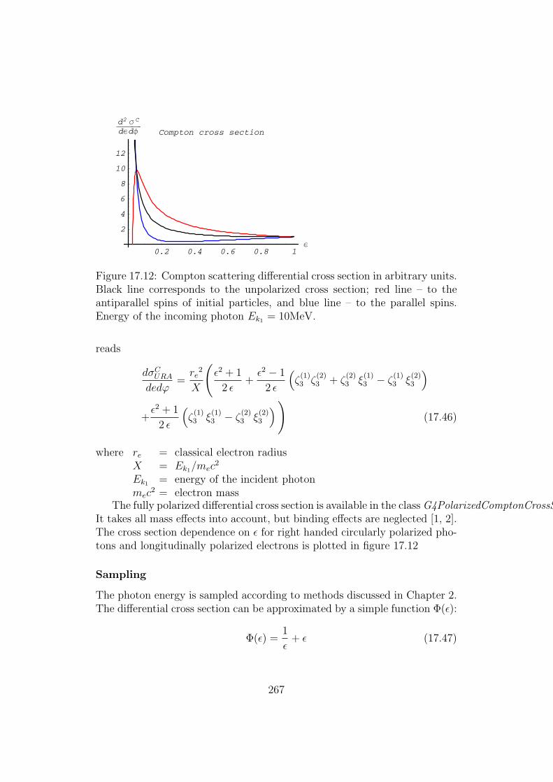
0.2 0.4 0.6 0.8 1Ε

2

4

6

8

10

12

d2 Σ C

dΕdΦ Compton cross section

Figure 17.12: Compton scattering differential cross section in arbitrary units.Black line corresponds to the unpolarized cross section; red line – to theantiparallel spins of initial particles, and blue line – to the parallel spins.Energy of the incoming photon Ek1 = 10MeV.

reads

dσCURA

dedϕ=re

2

X

(

ǫ2 + 1

2 ǫ+ǫ2 − 1

2 ǫ

(

ζ(1)3 ζ

(2)3 + ζ

(2)3 ξ

(1)3 − ζ

(1)3 ξ

(2)3

)

+ǫ2 + 1

2 ǫ

(

ζ(1)3 ξ

(1)3 − ζ

(2)3 ξ

(2)3

)

)

(17.46)

where re = classical electron radiusX = Ek1/mec

2

Ek1 = energy of the incident photonmec

2 = electron massThe fully polarized differential cross section is available in the classG4PolarizedComptonCrossSe

It takes all mass effects into account, but binding effects are neglected [1, 2].The cross section dependence on ǫ for right handed circularly polarized pho-tons and longitudinally polarized electrons is plotted in figure 17.12

Sampling

The photon energy is sampled according to methods discussed in Chapter 2.The differential cross section can be approximated by a simple function Φ(ǫ):

Φ(ǫ) =1

ǫ+ ǫ (17.47)

267

0.2 0.4 0.6 0.8 1Ε

-75

-50

-25

25

50

75

100

A, % Compton asymmetries

Figure 17.13: Compton scattering differential cross section asymmetries in%.Red line corresponds to the asymmetry due to circular photon and longitudi-nal electron initial state polarization, green line – due to circular photon andtransverse electron initial state polarization, blue line – due to linear photonand transverse electron initial state polarization.


ǫmin =1

1 + 2X(17.48)

ǫmax = 1 (17.49)

The kinematic of the scattered photon is constructed by the followingsteps:

1. ǫ is sampled from Φ(ǫ)

2. calculate the differential cross section, depending on the initial polar-izations ζ(1) and ζ(2), which the correct normalization.

3. ǫ is accepted with the probability defined by ratio of the differentialcross section over the approximation function.


5. ϕ is determined from the differential cross section, depending on theinitial polarizations ζ(1) and ζ(2).

In figure 17.13 the asymmetries indicate the influence of polarization for an10MeV incoming positron. The actual behavior is very sensitive to energy ofthe incoming positron.

268


After the kinematics is fixed the polarization of the outgoing photon is de-termined. Using the dependence of the differential cross section on the finalstate polarizations a mean polarization is calculated for each photon accord-ing to the method described in section 17.1.

The resulting polarization transfer functions ξ(1,2)(ǫ) are depicted in figure17.14.

0.2 0.4 0.6 0.8 1Ε

-1

-0.5

0.5

1

Γ: Circ=1, e-: POL=1

0.2 0.4 0.6 0.8 1Ε

-1

-0.5

0.5

1

Γ: Circ=-1, e-: POL=0

Figure 17.14: Polarization Transfer in Compton scattering. Blue line corre-sponds to the longitudinal polarization ξ

(2)3 of the electron, red line – circular

polarization ξ(1)3 of the photon.

Bibliography


[2] F.W. Lipps, H.A. Tolhoek, Physica 20 (1954) 85; F.W. Lipps, H.A. Tol-hoek, Physica 20 (1954) 395.

269

17.5 Polarized Bremsstrahlung for electron

and positron

17.5.1 Method

The polarized version of Bremsstrahlung is based on the unpolarized crosssection. Energy loss, mean free path, and distribution of explicitly generatedfinal state particles are treated by the unpolarized versionG4eBremsstrahlung.For details consult section 8.2.

The remaining task is to attribute polarization vectors to the generatedfinal state particles, which is discussed in the following.

17.5.2 Polarization in gamma conversion and brems-strahlung

Gamma conversion and bremsstrahlung are cross-symmetric processes (i.e.the Feynman diagram for electron bremsstrahlung can be obtained from thegamma conversion diagram by flipping the incoming photon and outgoingpositron lines) and their cross sections closely related. For both processes,the interaction occurs in the field of the nucleus and the total and differentialcross section are polarization independent. Therefore, only the polarizationtransfer from the polarized incoming particle to the outgoing particles istaken into account.

e−

N1 N2

q

ke− P−

P’−

N1 N2

k

q

P+

P−

e+

e−

Gamma conversion Bremsstrahlung

Figure 17.15: Feynman diagrams of Gamma conversion and bremsstrahlungprocesses.

For both processes, the scattering can be formulated by:

K1(k1, ζ(1)) +N1(kN1 , ζ

(N1)) −→ P1(p1, ξ(1)) + P2(p2, ξ

(2)) +N2(pN2 , ξ(N2))

(17.50)Where N1(kN1 , ζ

(N1)) and N2(pN2 , ξ(N2)) are the initial and final state of

the field of the nucleus respectively assumed to be unchanged, at rest andunpolarized. This leads to kN1 = kN2 = 0 and ζ(N1) = ξ(N2) = 0

270

In the case of gamma conversion process:K1(k1, ζ

(1)) is the incoming photon initial state with momentum k1 and po-larization state ζ(1).P1(p1, ξ

(1)) and P2(p2, ξ(2)) are the two photons final states with momenta

p1 and p2 and polarization states ξ(1) and ξ(2).In the case of bremsstrahlung process:

K1(k1, ζ(1)) is the incoming lepton e−(e+) initial state with momentum k1

and polarization state ζ(1).P1(p1, ξ

(1)) is the lepton e−(e+) final state with momentum p1 and polariza-tion state ξ(1).P2(p2, ξ

(2)) is the bremsstrahlung photon in final state with momentum p2and polarization state ξ(2).

17.5.3 Polarization transfer from the lepton e−(e+) toa photon

The polarization transfer from an electron (positron) to a photon in a brems-strahlung process was first calculated by Olsen and Maximon [1] taking intoaccount both Coulomb and screening effects. In the Stokes vector formalism,the e−(e+) polarization state can be transformed to a photon polarizationfinale state by means of interaction matrix T b

γ . It defined via

(

O

ξ(2)

)

= T bγ

(

1

ζ(1)

)

, (17.51)

and

T bγ ≈

1 0 0 0D 0 0 00 0 0 00 T 0 L

, (17.52)

where

I = (ǫ21 + ǫ22)(3 + 2Γ)− 2ǫ1ǫ2(1 + 4u2ξ2Γ) (17.53)

D =

8ǫ1ǫ2u2ξ2Γ

/I (17.54)

T =

−4kǫ2ξ(1− 2ξ)uΓ

/I (17.55)

L = k(ǫ1 + ǫ2)(3 + 2Γ)− 2ǫ2(1 + 4u2ξ2Γ)/I (17.56)

and

271

ǫ1 Total energy of the incoming lepton e+(e−) in units mc2

ǫ2 Total energy of the outgoing lepton e+(e−) in units mc2

k = (ǫ1 − ǫ2), the energy of the bremsstrahlung photon in units of mc2

p Electron (positron) initial momentum in units mck Bremsstrahlung photon momentum in units mcu Component of p perpendicular to k in units mc and u = |u|ξ = 1/(1 + u2)

Coulomb and screening effects are contained in Γ, defined as follows

Γ = ln

(

1

δ

)

− 2− f(Z) + F(

ξ

δ

)

for ∆ ≤ 120 (17.57)

Γ = ln

(

111

ξZ13

)

− 2− f(z) for ∆ ≥ 120 (17.58)

with

∆ =12Z

13 ǫ1ǫ2ξ

121kwith Z the atomic number and δ =

k

2ǫ1ǫ2(17.59)

f(Z) is the coulomb correction term derived by Davies, Bethe and Maxi-mon [6]. F(ξ/δ) contains the screening effects and is zero for ∆ ≤ 0.5 (Noscreening effects). For 0.5 ≤ ∆ ≤ 120 (intermediate screening) it is a slowlydecreasing function. The F(ξ/δ) values versus ∆ are given in table 17.1 andused with a linear interpolation in between.

The polarization vector of the incoming e−(e+) must be rotated into theframe defined by the scattering plane (x-z-plane) and the direction of the out-going photon (z-axis). The resulting polarization vector of the bremsstrahlungphoton is also given in this frame. Using Eq. (17.51) and the transfer matrixgiven by Eq. (17.52) the bremsstrahlung photon polarization state in theStokes formalism [2, 3] is given by

ξ(2) =

ξ(2)1

ξ(2)2

ξ(2)3

≈

D0

ζ(1)1 L+ ζ

(1)2 T

(17.60)

17.5.4 Remaining polarization of the lepton after emit-ting a bremsstrahlung photon

The e−(e+) polarization final state after emitting a bremsstrahlung photoncan be calculated using the interaction matrix T b

l which describes the lepton

272

Table 17.1: F(ξ/δ) for intermediate values of the screening factor [7].

∆ −F(

ξ/δ)

∆ −F(

ξ/δ)

0.5 0.0145 40.0 2.001.0 0.0490 45.0 2.1142.0 0.1400 50.0 2.2164.0 0.3312 60.0 2.3938.0 0.6758 70.0 2.54515.0 1.126 80.0 2.67620.0 1.367 90.0 2.79325.0 1.564 100.0 2.89730.0 1.731 120.0 3.07835.0 1.875

depolarization. The polarization vector for the outgoing e−(e+) is not givenby Olsen and Maximon. However, their results can be used to calculate thefollowing transfer matrix [4, 5].

(

O

ξ(1)

)

= T bl

(

1

ζ(1)

)

(17.61)

T bl ≈

1 0 0 0D M 0 E0 0 M 00 F 0 M + P

(17.62)

where

I = (ǫ21 + ǫ22)(3 + 2Γ)− 2ǫ1ǫ2(1 + 4u2ξ2Γ) (17.63)

F = ǫ2

4kξu(1− 2ξ)Γ

/I (17.64)

E = ǫ1

4kξu(2ξ − 1)Γ

/I (17.65)

M =

4kǫ1ǫ2(1 + Γ− 2u2ξ2Γ)

/I (17.66)

P =

k2(1 + 8Γ(ξ − 0.5)2

/I (17.67)

and

273

ǫ1 Total energy of the incoming e+/e− in units mc2

ǫ2 Total energy of the outgoing e+/e− in units mc2

k = (ǫ1 − ǫ2), energy of the photon in units of mc2

p Electron (positron) initial momentum in units mck Photon momentum in units mcu Component of p perpendicular to k in units mc and u = |u|

Using Eq. (17.61) and the transfer matrix given by Eq. (17.62) the e−(e+)polarization state after emitting a bremsstrahlung photon is given in theStokes formalism by

ξ(1) =

ξ(1)1

ξ(1)2

ξ(1)3

≈

ζ(1)1 M + ζ

(1)3 E

ζ(1)2 M

ζ(1)3 (M + P ) + ζ

(1)1 F

. (17.68)

Bibliography

[1] H. Olsen and L.C. Maximon. Photon and electron polarization in high-energy bremsstrahlung and pair production with screening. Physical Re-view, 114:887-904, 1959.

[2] W.H. McMaster. Polarization and the Stokes parameters. American Jour-nal of Physics, 22(6):351-362, 1954.

[3] W.H. McMaster. Matrix representation of polarization. Reviews of Mod-ern Physics, 33(1):8-29, 1961.

[4] K. Flottmann. Investigations toward the development of polarized andunpolarized high intensity positron sources for linear colliders. PhD the-sis, Universitat Hamburg, 1993.

[5] Hoogduin, Johannes Marinus, Electron, positron and photon polarimetry.PhD thesis, Rijksuniversiteit Groningen 1997.

[6] H. Davies, H.A. Bethe and L.C. Maximon, Theory of Bremsstrahlung andPair Production. II. Integral Cross Section for Pair Production, PhysicalReview, 93(4):788-795, 1954.

[7] H.W. Koch and J.W. Motz, Bremsstrahlung cross-section formulas andrelated data. Review Mod. Phys., 31(4):920-955, 1959.

[8] K. Laihem, PhD thesis, Measurement of the positron polarization at anhelical undulator based positron source for the International Linear Col-lider ILC, Humboldt University Berlin, Germany, (2008).

274

17.6 Polarized Gamma conversion into an electron–

positron pair

17.6.1 Method

The polarized version of gamma conversion is based on the EM standard pro-cess G4GammaConversion. Mean free path and the distribution of explicitlygenerated final state particles are treated by this version. For details consultsection 5.4.

The remaining task is to attribute polarization vectors to the generatedfinal state leptons, which is discussed in the following.

17.6.2 Polarization transfer from the photon to thetwo leptons

Gamma conversion process is essentially the inverse process of Bremsstrahlungand the interaction matrix is obtained by inverting the rows and columns ofthe bremsstrahlung matrix and changing the sign of ǫ2, cf. section 17.5. Itfollows from the work by Olsen and Maximon [1] that the polarization stateξ(1) of an electron or positron after pair production is obtained by

(

O

ξ(1)

)

= T pl

(

1

ζ(1)

)

(17.69)

and

T pl ≈

1 D 0 00 0 0 T0 0 0 00 0 0 L

, (17.70)

where

I = (ǫ21 + ǫ22)(3 + 2Γ) + 2ǫ1ǫ2(1 + 4u2ξ2Γ) (17.71)

D =

−8ǫ1ǫ2u2ξ2Γ

/I (17.72)

T =

−4kǫ2ξ(1− 2ξ)uΓ

/I (17.73)

L = k(ǫ1 − ǫ2)(3 + 2Γ) + 2ǫ2(1 + 4u2ξ2Γ)/I (17.74)

and

275

ǫ1 total energy of the first lepton e+(e−) in units mc2

ǫ2 total energy of the second lepton e−(e+) in units mc2

k = (ǫ1 + ǫ2) energy of the incoming photon in units of mc2

p electron=positron initial momentum in units mck photon momentum in units mcu electron/positron initial momentum in units mcu = |u|

Coulomb and screening effects are contained in Γ, defined in section 17.5.Using Eq. (17.69) and the transfer matrix given by Eq. (17.70) the polar-

ization state of the produced e−(e+) is given in the Stokes formalism by:

ξ(1) =

ξ(1)1

ξ(1)2

ξ(1)3

≈

ζ(1)3 T0

ζ(1)3 L

(17.75)

Bibliography

[1] H. Olsen and L.C. Maximon. Photon and electron polarization in high-energy bremsstrahlung and pair production with screening. Physical Re-view, 114:887-904, 1959.


276

17.7 Polarized Photoelectric Effect

17.7.1 Method

This section describes the basic formulas of polarization transfer in the pho-toelectric effect class (G4PolarizedPhotoElectricEffect). The photoelectriceffect is the emission of electrons from matter upon the absorption of elec-tromagnetic radiation, such as ultraviolet radiation or x-rays. The energyof the photon is completely absorbed by the electron and, if sufficient, theelectron can escape from the material with a finite kinetic energy. A singlephoton can only eject a single electron, as the energy of one photon is onlyabsorbed by one electron. The electrons that are emitted are often calledphotoelectrons. If the photon energy is higher than the binding energy theremaining energy is transferred to the electron as a kinetic energy

Ee−kin = k −Bshell (17.76)

In Geant4 the photoelectric effect process is taken into account if:

k > Bshell (17.77)

Where k is the incoming photon energy and Bshell the electron binding energyprovided by the class G4AtomicShells.

The polarized version of the photoelectric effect is based on the EM stan-dard process G4PhotoElectricEffect. Mean free path and the distributionof explicitly generated final state particles are treated by this version. Fordetails consult section 5.2.

The remaining task is to attribute polarization vectors to the generatedfinal state electron, which is discussed in the following.

17.7.2 Polarization transfer

The polarization state of an incoming polarized photon is described by theStokes vector ~ζ(1). The polarization transfer to the photoelectron can be de-scribed in the Stokes formalism using the same approach as for the Bremsstrahlungand gamma conversion processes, cf. 17.5 and 17.6. The relation between thephotoelectron’s Stokes parameters and the incoming photon’s Stokes param-eters is described by the interaction matrix T p

l derived from H. Olsen [1] andreviewed by H.W McMaster [2]:

(

I ′

~ξ(1)

)

= T pl

(

I0~ζ(1)

)

(17.78)

277

In general, for the photoelectric effect as a two-body scattering, the crosssection should be correlated with the spin states of the incoming photonand the target electron. In our implementation the target electron is notpolarized and only the polarization transfer from the photon to the pho-toelectron is taken into account. In this case the cross section of the pro-cess remains polarization independent. To compute the matrix elements wetake advantage of the available kinematic variables provided by the genericG4PhotoelectricEffect class. To compute the photoelectron spin state (Stokesparameters), four main parameters are needed:

• The incoming photon Stokes vector ~ζ(1)

• The incoming photon’s energy k.

• the photoelectron’s kinetic energy Ee−kin or the Lorentz factors β and γ.

• The photoelectron’s polar angle θ or cos θ.

The interaction matrix derived by H. Olsen [1] is given by:

T Pl =

1 +D −D 0 00 0 0 B0 0 0 00 0 0 A

(17.79)

Where

D =1

k

[

2

kǫ(1− β cos θ)− 1

]

(17.80)

A =ǫ

ǫ+ 1

[

2

kǫ+ β cos θ +

2

kǫ2(1− β cos θ)

]

(17.81)

B =ǫ

ǫ+ 1β sin θ

[

2

kǫ(1− β cos θ)− 1

]

(17.82)

Using Eq. (17.78) and the transfer matrix given by Eq. (17.79) the polar-ization state of the produced e− is given in the Stokes formalism by:

~ξ(1) =

ξ(1)1

ξ(1)2

ξ(1)3

=

ζ(1)3 B0

ζ(1)3 A

(17.83)

From equation (17.83) one can see that a longitudinally (transversally)polarized photoelectron can only be produced if the incoming photon is cir-cularly polarized.

278

Bibliography

[1] H. Olsen, Kgl. N. Videnskab. Selskabs Forh. 31, Nos 11, 11a (1958).

[2] W.H. McMaster. Matrix representation of polarization. Reviews of Mod-ern Physics, 33(1):8-29, 1961.


279

Chapter 18

X-Ray Production

280

18.1 Transition radiation

18.1.1 The Relationship of Transition Radiation to X-ray Cherenkov Radiation

X-ray transition radiation (XTR ) occurs when a relativistic charged particlepasses from one medium to another of a different dielectric permittivity. Inorder to describe this process it is useful to begin with an explanation ofX-ray Cherenkov radiation, which is closely related.

The mean number of X-ray Cherenkov radiation (XCR) photons of fre-quency ω emitted into an angle θ per unit distance along a particle trajectoryis [1]

d3Nxcr

~dω dx dθ2=

α

π~c

ω

cθ2Im Z . (18.1)

Here the quantity Z is introduced as the complex formation zone of XCR inthe medium:

Z =L

1− iL

l

, L =c

ω

[

γ−2 +ω2p

ω2+ θ2

]−1

, γ−2 = 1− β2. (18.2)

with l and ωp the photon absorption length and the plasma frequency, re-spectively, in the medium. For the case of a transparent medium, l → ∞and the complex formation zone reduces to the coherence length L of XCR.The coherence length roughly corresponds to that part of the trajectory inwhich an XCR photon can be created.

Introducing a complex quantity Z with its imaginary part proportionalto the absorption cross-section (∼ l−1) is required in order to account forabsorption in the medium. Usually, ω2

p/ω2 ≫ c/ωl. Then it can be seen from

Eqs. 18.1 and 18.2 that the number of emitted XCR photons is considerablysuppressed and disappears in the limit of a transparent medium. This iscaused by the destructive interference between the photons emitted fromdifferent parts of the particle trajectory.

The destructive interference of X-ray Cherenkov radiation is removed ifthe particle crosses a boundary between two media with different dielectricpermittivities, ǫ, where

ǫ = 1− ω2p

ω2+ i

c

ωl. (18.3)

Here the standard high-frequency approximation for the dielectric permittiv-ity has been used. This is valid for energy transfers larger than the K-shellexcitation potential.

281

If layers of media are alternated with spacings of order L, the X-rayradiation yield from a trajectory of unit length can be increased by roughlyl/L times. The radiation produced in this case is called X-ray transitionradiation (XTR).

18.1.2 Calculating the X-ray Transition Radiation Yield

Using the methods developed in Ref. [2] one can derive the relation describingthe mean number of XTR photons generated per unit photon frequency andθ2 inside the radiator for a general XTR radiator consisting of n differentabsorbing media with fluctuating thicknesses:

d2Nin

~dω dθ2=

α

π~c2ωθ2Re

n−1∑

i=1

(Zi − Zi+1)2+ (18.4)

+ 2n−1∑

k=1

k−1∑

i=1

(Zi − Zi+1)

[

k∏

j=i+1

Fj

]

(Zk − Zk+1)

, Fj = exp

[

− tj2Zj

]

.

In the case of gamma distributed gap thicknesses (foam or fiber radiators)the values Fj, (j = 1, 2) can be estimated as:

Fj =

∫ ∞

0

dtj

(

νjtj

)νj tνj−1j

Γ(νj)exp

[

−νjtjtj

− itj2Zj

]

=

[

1 + itj

2Zjνj

]−νj

,

(18.5)where Zj is the complex formation zone of XTR (similar to relation 18.2for XCR) in the j-th medium [2, 6]. Γ is the Euler gamma function, tj isthe mean thickness of the j-th medium in the radiator and νj > 0 is theparameter roughly describing the relative fluctuations of tj. In fact, therelative fluctuation is δtj/tj ∼ 1/

√νj.

In the particular case of n foils of the first medium (Z1, F1) interspersedwith gas gaps of the second medium (Z2, F2), one obtains:

d2Nin

~dω dθ2=

2α

π~c2ωθ2Re

〈R(n)〉

, F = F1F2, (18.6)

〈R(n)〉 = (Z1 − Z2)2

n(1− F1)(1− F2)

1− F+

(1− F1)2F2[1− F n]

(1− F )2

. (18.7)

Here 〈R(n)〉 is the stack factor reflecting the radiator geometry. The integra-tion of (18.6) with respect to θ2 can be simplified for the case of a regularradiator (ν1,2 → ∞), transparent in terms of XTR generation media, and

282

n≫ 1 [3]. The frequency spectrum of emitted XTR photons is given by:

dNin

~dω=

∫ ∼10γ−2

0

dθ2d2Nin

~dω dθ2=

4αn

π~ω(C1 + C2)

2

·kmax∑

k=kmin

(k − Cmin)

(k − C1)2(k + C2)2sin2

[

πt1t1 + t2

(k + C2)

]

,

(18.8)

C1,2 =t1,2(ω

21 − ω2

2)

4πcω, Cmin =

1

4πc

[

ω(t1 + t2)

γ2+t1ω

21 + t2ω

22

ω

]

.

The sum in (18.8) is defined by terms with k ≥ kmin corresponding to theregion of θ ≥ 0. Therefore kmin should be the nearest to Cmin integer kmin ≥Cmin. The value of kmax is defined by the maximum emission angle θ2max ∼10γ−2. It can be evaluated as the integer part of

Cmax = Cmin +ω(t1 + t2)

4πc

10

γ2, kmax − kmin ∼ 102 ÷ 103 ≫ 1.

Numerically, however, only a few tens of terms contribute substantially to thesum, that is, one can choose kmax ∼ kmin + 20. Equation (18.8) correspondsto the spectrum of the total number of photons emitted inside a regulartransparent radiator. Therefore the mean interaction length, λXTR, of theXTR process in this kind of radiator can be introduced as:

λXTR = n(t1 + t2)

[∫

~ωmax

~ωmin

~dωdNin

~dω

]−1

,

where ~ωmin ∼ 1 keV, and ~ωmax ∼ 100 keV for the majority of high energyphysics experiments. Its value is constant along the particle trajectory inthe approximation of a transparent regular radiator. The spectrum of thetotal number of XTR photons after regular transparent radiator is definedby (18.8) with:

n→ neff =n−1∑

k=0

exp[−k(σ1t1 + σ2t2)] =1− exp[−n(σ1t1 + σ2t2)]

1− exp[−(σ1t1 + σ2t2)],

where σ1 and σ2 are the photo-absorption cross-sections corresponding to thephoton frequency ω in the first and the second medium, respectively. Withthis correction taken into account the XTR absorption in the radiator (18.8)corresponds to the results of [4]. In the more general case of the flux of XTR

283

photons after a radiator, the XTR absorption can be taken into account witha calculation based on the stack factor derived in [5]:

〈R(n)flux〉 = (L1 − L2)

2

1−Qn

1−Q

(1 +Q1)(1 + F )− 2F1 − 2Q1F2

2(1− F )

+(1− F1)(Q1 − F1)F2(Q

n − F n)

(1− F )(Q− F )

, (18.9)

Q = Q1 ·Q2, Qj = exp [−tj/lj ] = exp [−σjtj] , j = 1, 2.

Both XTR energy loss (18.7) and flux (18.9) models can be implemented asa discrete electromagnetic process (see below).

18.1.3 Simulating X-ray Transition Radiation Produc-tion

A typical XTR radiator consits of many (∼ 100) boundaries between differentmaterials. To improve the tracking performance in such a volume one canintroduce an artificial material [6], which is the geometrical mixture of foiland gas contents. Here is an example:

// In DetectorConstruction of an application

// Preparation of mixed radiator material

foilGasRatio = fRadThickness/(fRadThickness+fGasGap);

foilDensity = 1.39*g/cm3; // Mylar

gasDensity = 1.2928*mg/cm3 ; // Air

totDensity = foilDensity*foilGasRatio +

gasDensity*(1.0-foilGasRatio);

fractionFoil = foilDensity*foilGasRatio/totDensity;

fractionGas = gasDensity*(1.0-foilGasRatio)/totDensity;

G4Material* radiatorMat = new G4Material("radiatorMat",

totDensity,

ncomponents = 2 );

radiatorMat->AddMaterial( Mylar, fractionFoil );

radiatorMat->AddMaterial( Air, fractionGas );

G4cout << *(G4Material::GetMaterialTable()) << G4endl;

// materials of the TR radiator

fRadiatorMat = radiatorMat; // artificial for geometry

fFoilMat = Mylar;

fGasMat = Air;

This artificial material will be assigned to the logical volume in whichXTR will be generated:

284

solidRadiator = new G4Box("Radiator",

1.1*AbsorberRadius ,

1.1*AbsorberRadius,

0.5*radThick );

logicRadiator = new G4LogicalVolume( solidRadiator,

fRadiatorMat, // !!!

"Radiator");

physiRadiator = new G4PVPlacement(0,

G4ThreeVector(0,0,zRad),

"Radiator", logicRadiator,

physiWorld, false, 0 );

XTR photons generated by a relativistic charged particle intersecting aradiator with 2n interfaces between different media can be simulated by usingthe following algorithm. First the total number of XTR photons is estimatedusing a Poisson distribution about the mean number of photons given by thefollowing expression:

N (n) =

∫ ω2

ω1

dω

∫ θ2max

0

dθ2d2N (n)

dω dθ2=

2α

πc2

∫ ω2

ω1

ωdω

∫ θ2max

0

θ2dθ2Re

〈R(n)〉

.

Here θ2max ∼ 10γ−2, ~ω1 ∼ 1 keV, ~ω2 ∼ 100 keV, and 〈R(n)〉 correspond tothe geometry of the experiment. For events in which the number of XTRphotons is not equal to zero, the energy and angle of each XTR quantum issampled from the integral distributions obtained by the numerical integrationof expression (18.6). For example, the integral energy spectrum of emitted

XTR photons, N(n)>ω , is defined from the following integral distribution:

N(n)>ω =

2α

πc2

∫ ω2

ω

ωdω

∫ θ2max

0

θ2dθ2Re

〈R(n)〉

.

In Geant4 XTR generation inside or after radiators is described as a dis-crete electromagnetic process. It is convenient for the description of tracks inmagnetic fields and can be used for the cases when the radiating charge ex-periences a scattering inside the radiator. The base class G4VXTRenergyLossis responsible for the creation of tables with integral energy and angulardistributions of XTR photons. It also contains the PostDoIt function pro-viding XTR photon generation and motion (if fExitFlux=true) through aXTR radiator to its boundary. Particular models like G4RegularXTRadiatorimplement the pure virtual function GetStackFactor, which calculates theresponse of the XTR radiator reflecting its geometry. Included below aresome comments for the declaration of XTR in a user application.

285

In the physics list one should pass to the XTR process additional detailsof the XTR radiator involved:

// In PhysicsList of an application

else if (particleName == "e-") // Construct processes for electron with XTR

pmanager->AddProcess(new G4MultipleScattering, -1, 1,1 );

pmanager->AddProcess(new G4eBremsstrahlung(), -1,-1,1 );

pmanager->AddProcess(new Em10StepCut(), -1,-1,1 );

// in regular radiators:

pmanager->AddDiscreteProcess(

new G4RegularXTRadiator // XTR dEdx in general regular radiator

// new G4XTRRegularRadModel - XTR flux after general regular radiator

// new G4TransparentRegXTRadiator - XTR dEdx in transparent

// regular radiator

// new G4XTRTransparentRegRadModel - XTR flux after transparent

// regular radiator

(pDet->GetLogicalRadiator(), // XTR radiator

pDet->GetFoilMaterial(), // real foil

pDet->GetGasMaterial(), // real gas

pDet->GetFoilThick(), // real geometry

pDet->GetGasThick(),

pDet->GetFoilNumber(),

"RegularXTRadiator"));

// or for foam/fiber radiators:

pmanager->AddDiscreteProcess(

new G4GammaXTRadiator - XTR dEdx in general foam/fiber radiator

// new G4XTRGammaRadModel - XTR flux after general foam/fiber radiator

( pDet->GetLogicalRadiator(),

1000.,

100.,

pDet->GetFoilMaterial(),

pDet->GetGasMaterial(),

pDet->GetFoilThick(),

pDet->GetGasThick(),

pDet->GetFoilNumber(),

"GammaXTRadiator"));

Here for the foam/fiber radiators the values 1000 and 100 are the ν parame-ters (which can be varied) of the Gamma distribution for the foil and gas gaps,

286

respectively. Classes G4TransparentRegXTRadiator and G4XTRTransparentRegRadModelcorrespond (18.8) to n and neff , respectively.

Bibliography

[1] V.M. Grichine, Nucl. Instr. and Meth., A482 (2002) 629.

[2] V.M. Grichine, Physics Letters, B525 (2002) 225-239

[3] G.M. Garibyan, Sov. Phys. JETP 32 (1971) 23.

[4] C.W. Fabian and W. Struczinski Physics Letters, B57 (1975) 483.

[5] G.M. Garibian, L.A. Gevorgian, and C. Yang, Sov. Phys.- JETP, 39(1975) 265.

[6] J. Apostolakis, S. Giani, V. Grichine et al., Comput. Phys. Commun.132 (2000) 241.

287

18.2 Scintillation

Every scintillating material has a characteristic light yield, Y (photons/MeV ),and an intrinsic resolution which generally broadens the statistical distribu-tion, σi/σs > 1, due to impurities which are typical for doped crystals likeNaI(Tl) and CsI(Tl). The average yield can have a non-linear dependenceon the local energy deposition. Scintillators also have a time distributionspectrum with one or more exponential decay time constants, τi, with eachdecay component having its intrinsic photon emission spectrum. These areempirical parameters typical for each material.

The generation of scintillation light can be simulated by sampling the numberof photons from a Poisson distribution. This distribution is based on theenergy lost during a step in a material and on the scintillation properties ofthat material. The frequency of each photon is sampled from the empiricalspectra. The photons are generated evenly along the track segment and areemitted uniformly into 4π with a random linear polarization.

288

18.3 Cerenkov Effect

The radiation of Cerenkov light occurs when a charged particle moves througha dispersive medium faster than the speed of light in that medium. A dis-persive medium is one whose index of refraction is an increasing function ofphoton energy. Two things happen when such a particle slows down:

1. a cone of Cerenkov photons is emitted, with the cone angle (measuredwith respect to the particle momentum) decreasing as the particle losesenergy;

2. the momentum of the photons produced increases, while the numberof photons produced decreases.

When the particle velocity drops below the local speed of light, photons areno longer emitted. At that point, the Cerenkov cone collapses to zero.

In order to simulate Cerenkov radiation the number of photons per tracklength must be calculated. The formulae used for this calculation can befound below and in [1, 2]. Let n be the refractive index of the dielectricmaterial acting as a radiator. Here n = c/c′ where c′ is the group velocity oflight in the material, hence 1 ≤ n. In a dispersive material n is an increasingfunction of the photon energy ǫ (dn/dǫ ≥ 0). A particle traveling with speedβ = v/c will emit photons at an angle θ with respect to its direction, whereθ is given by

cos θ =1

βn.

From this follows the limitation for the momentum of the emitted photons:

n(ǫmin) =1

β.

Photons emitted with an energy beyond a certain value are immediatelyre-absorbed by the material; this is the window of transparency of the radi-ator. As a consequence, all photons are contained in a cone of opening anglecos θmax = 1/(βn(ǫmax)).

The average number of photons produced is given by the relations :

dN =αz2

~csin2 θdǫdx =

αz2

~c(1− 1

n2β2)dǫdx

≈ 370z2photons

eV cm(1− 1

n2β2)dǫdx

289

and the number of photons generated per track length is

dN

dx≈ 370z2

∫ ǫmax

ǫmin

dǫ

(

1− 1

n2β2

)

= 370z2[

ǫmax − ǫmin −1

β2

∫ ǫmax

ǫmin

dǫ

n2(ǫ)

]

.

The number of photons produced is calculated from a Poisson distributionwith a mean of 〈n〉 = StepLength dN/dx. The energy distribution of thephoton is then sampled from the density function

f(ǫ) =

[

1− 1

n2(ǫ)β2

]

.

Bibliography

[1] J.D.Jackson, Classical Electrodynamics, John Wiley and Sons (1998)

[2] D.E. Groom et al. Particle Data Group . Rev. of Particle Properties.Eur. Phys. J. C15,1 (2000) http://pdg.lbl.gov/

290

18.4 Synchrotron Radiation

18.4.1 Photon spectrum

Synchrotron radiation photons are emitted by relativistic charged particlestraveling in magnetic fields. The properties of synchrotron radiation are wellunderstood and described in textbooks [1, 2, 3].

In the simplest case, we have an electron of momentum p moving perpen-dicular to a homogeneous magnetic field B. The magnetic field will keep theparticle on a circular path, with radius

ρ =p

eB=mγβc

eB. Numerically we have ρ[m] = p[GeV/c]

3.336m

B[T].

(18.10)In general, there will be an arbitrary angle θ between the local magneticfield B and momentum vector p of the particle. The motion has a circularcomponent in the plane perpendicular to the magnetic field, and in addition aconstant momentum component parallel to the magnetic field. For a constanthomogeneous field, the resulting trajectory is a helix.

The critical energy of the synchrotron radiation can be calculated usingthe radius ρ of Eq.18.10 and angle θ or the magnetic field perpendicular tothe particle direction B⊥ = B sin θ according to

Ec =3

2~cγ3 sin θ

ρ=

3 ~

2mγ2 eB⊥ . (18.11)

Half of the synchrotron radiation power is radiated by photons above thecritical energy.

With x we denote the photon energy Eγ, expressed in units of the criticalenergy Ec

x =Eγ

Ec

. (18.12)

The photon spectrum (number of photons emitted per path length s andrelative energy x) can be written as

d2N

ds dx=

√3α

2π

eB⊥mc

∫ ∞

x

K5/3(ξ) dξ (18.13)

where α = e2/ 4πǫ0~c is the dimensionless electromagnetic coupling (or finestructure) constant andK5/3 is the modified Bessel function of the third kind.

The number of photons emitted per unit length and the mean free pathλ between two photon emissions is obtained by integration over all photon

291

energies. Using∫ ∞

0

dx

∫ ∞

x

K5/3(ξ) dξ =5π

3(18.14)

we find thatdN

ds=

5α

2√3

eB⊥mβc

=1

λ. (18.15)

Here we are only interested in ultra-relativistic (β ≈ 1) particles, forwhich λ only depends on the field B and not on the particle energy. Wedefine a constant λB such that

λ =λBB⊥

where λB =2√3

5

mc

α e= 0.16183Tm . (18.16)

As an example, consider a 10GeV electron, travelling perpendicular toa 1T field. It moves along a circular path of radius ρ = 33.356m. For theLorentz factor we have γ = 19569.5 and β = 1−1.4×10−9. The critical energyis Ec = 66.5 keV and the mean free path between two photon emissions isλ = 0.16183m.

18.4.2 Validity

The spectrum given in Eq. 18.13 can generally be expected to provide a veryaccurate description for the synchrotron radiation spectrum generated byGeV electrons in magnetic fields.

Here we discuss some known limitations and possible extensions.For particles traveling on a circular path, the spectrum observed in one

location will in fact not be a continuous spectrum, but a discrete spectrum,consisting only of harmonics or modes n of the revolution frequency. Inpractice, the mode numbers will generally be too high to make this a visibleeffect. The critical mode number corresponding to the critical energy isnc = 3/2 γ3. 10GeV electrons for example have nc ≈ 1013.

Synchrotron radiation can be neglected for slower particles and only be-comes relevant for ultra-relativistic particles with γ > 103. Using β = 1introduces an uncertainty of about 1/2γ2 or less than 5× 10−7.

It is rather straightforward to extend the formulas presented here to par-ticles other than electrons, with arbitrary charge q and mass m, see [4]. Thenumber of photons and the power scales with the square of the charge.

The standard synchrotron spectrum of Eq. 18.13 is only valid as long asthe photon energy remains small compared to the particle energy [5, 6]. Thisis a very safe assumption for GeV electrons and standard magnets with fieldsof order of Tesla.

292

An extension of synchrotron radiation to fields exceeding several hundredTesla, such as those present in the beam-beam interaction in linear-colliders,is also known as beamstrahlung. For an introduction see [7].

The standard photon spectrum applies to homogeneous fields and re-mains a good approximation for magnetic fields which remain approximatelyconstant over a the length ρ/γ, also known as the formation length for syn-chrotron radiation. Short magnets and edge fields will result instead in moreenergetic photons than predicted by the standard spectrum.

We also note that short bunches of many particles will start to radiatecoherently like a single particle of the equivalent charge at wavelengths whichare longer than the bunch dimensions.

Low energy, long-wavelength synchrotron radiation may destructively in-terfere with conducting surfaces [8].

The soft part of the synchrotron radiation spectrum emitted by chargedparticles travelling through a medium will be modified for frequencies closeto and lower than the plasma frequency [9].

18.4.3 Direct inversion and generation of the photonenergy spectrum

The task is to find an algorithm that effectively transforms the flat distri-bution given by standard pseudo-random generators into the desired distri-bution proportional to the expressions given in Eqs. 18.13, 18.17. The trans-formation is obtained from the inverse F−1 of the cumulative distributionfunction F (x) =

∫ x

0f(t)dt.

Leaving aside constant factors, the probability density function relevantfor the photon energy spectrum is

SynRad(x) =

∫ ∞

x

K5/3(t)dt . (18.17)

Numerical methods to evaluate K5/3 are discussed in [10]. An efficient al-gorithm to evaluate the integral SynRad using Chebyshev polynomials isdescribed in [11]. This has been used in an earlier version of the Monte Carlogenerator for synchrotron radiation using approximate transformations andthe rejection method [12].

The cumulative distribution function is the integral of the probabilitydensity function. Here we have

SynRadInt(z) =

∫ ∞

z

SynRad(x) dx , (18.18)

293

10- 7 0.00001 0.001 0.1 10.0.

0.2

0.4

0.6

0.8

1.

x

y

0. 0.2 0.4 0.6 0.8 1.10-7

10-5

0.001

0.1

10.x

y

Figure 18.1: SynFracInt (left) and its inverse InvSynFracInt (right), on alog x scale. The functions x1/3, y3 and 1 − e−x, − log(1 − y) are shown asdashed lines.

with normalization

SynRadInt(0) =

∫ ∞

0

SynRad(x) dx =5π

3, (18.19)

such that 35πSynRadInt(x) gives the fraction of photons above x.

It is possible to directly obtain the desired distribution with a fast andaccurate algorithm using an analytical description based on simple transfor-mations and Chebyshev polynomials. This approach is used here.

We now describe in some detail how the analytical description was ob-tained. For more details see [13].

It turned out to be convenient to start from the normalized complementrather then Eq. 18.18 directly, that is

SynFracInt(x) =3

5π

∫ x

0

∫ ∞

x

K5/3(t)dt dx = 1− 3

5πSynRadInt(x) , (18.20)

which gives the fraction of photons below x.Figure 18.1 shows on the left hand side y = SynFracInt(x) and on the

right hand side the inverse x = InvSynFracInt(y) together with simple ap-proximate functions. We can see, that SynFracInt can be approximated byx1/3 for small arguments, and by 1− e−x for large x. Consequently, we havefor the inverse, InvSynFracInt(y), which can be approximated for small y byy3 and for large y by − log(1− y).

Good convergence for InvSynFracInt(y) was obtained using Chebyshevpolynomials combined with the approximate expressions for small and largearguments. For intermediate values, a Chebyshev polynomial can be useddirectly. Table 18.1 summarizes the expressions used in the different intervals.

294

Table 18.1: InvSynFracInt.

y x = InvSynFracInt(y)y < 0.7 y3 PCh(y)

0.7 ≤ y ≤ 0.9999 PCh(y)y > 0.9999 − log(1− y)PCh(− log(1− y))

10 3

10 4

10 5

10 6

10 7

0 1 2 3 4 5

x = Eγ / Ec

phot

on s

pect

rum

dN

/dx

10 4

10 5

10 6

0 1 2 3 4 5

x = Eγ / Ec

pow

er s

pect

rum

x d

N/d

x

Figure 18.2: Comparison of the exact (smooth curve) and generated (his-togram) spectra for 2 × 107 events. The photon spectrum is shown on theleft and the power spectrum on the right side.

The procedure for Monte Carlo simulation is to generate y at random uni-formly distributed between 0 at 1, as provided by standard random gen-erators, and then to calculate the energy x in units of the critical energyaccording to x = InvSynFracInt(y).

The numerical accuracy of the energy spectrum presented here is about 14decimal places, close to the machine precision. Fig. 18.2 shows a comparisonof generated and expected spectra. A Geant4 display of an electron movingin a magnetic field radiating synchrotron photons is presented in Fig. 18.3

295

e+

-250 250

250

x [m]

y [m

]

-250

x

y

zB

Synchrotron radiation photons

Figure 18.3: Geant4 display. 10 GeV e+ moving initially in x-direction, bendsdownwards on a circular path by a 0.1T magnetic field in z-direction.

18.4.4 Properties of the Power Spectra

The normalised probability function describing the photon energy spectrumis

nγ(x) =3

5π

∫ ∞

x

K5/3(t)dt . (18.21)

nγ(x) gives the fraction of photons in the interval x to x + dx, where x isthe photon energy in units of the critical energy. The first moment or meanvalue is

µ =

∫ ∞

0

xnγ(x) dx =8

15√3. (18.22)

implying that the mean photon energy is 815

√3= 0.30792 of the critical en-

ergy.

The second moment about the mean, or variance, is

σ2 =

∫ ∞

0

(x− µ)2 nγ(x) dx =211

675, (18.23)

and the r.m.s. value of the photon energy spectrum is σ =√

211675

= 0.5591.

296

The normalised power spectrum is

Pγ(x) =9√3

8πx

∫ ∞

x

K5/3(t)dt . (18.24)

Pγ(x) gives the fraction of the power which is radiated in the interval x tox+ dx.

Half of the power is radiated below the critical energy

∫ 1

0

Pγ(x) dx = 0.5000 (18.25)

The mean value of the power spectrum is

µ =

∫ ∞

0

xPγ(x) dx =55

24√3= 1.32309 . (18.26)

The variance is

σ2 =

∫ ∞

0

(x− µ)2 Pγ(x) dx =2351

1728, (18.27)

and the r.m.s. width is σ =√

23511728

= 1.16642.

Bibliography

[1] A.A.Sokolov and I.M.Ternov, Radiation from Relativistic Electrons,Amer. Inst of Physics, 1986.

[2] J. Jackson, Classical Electrodynamics. John Wiley & Sons, third ed.,1998.

[3] A. Hofmann, The Physics of Synchrotron Radiation. Cambridge Uni-versity Press, 2004.

[4] H. Burkhardt, “Reminder of the Edge Effect in Synchrotron Radiation”,LHC Project Note 172, CERN Geneva 1998.

[5] F. Herlach, R. McBroom, T. Erber, J. .Murray, and R. Gearhart, “Ex-periments with Megagauss targets at SLAC”, IEEE Trans Nucl Sci, NS18, 3 (1971) 809-814.

[6] T. Erber, G. B. Baumgartner, D. White, and H. G. Latal, “MegagaussBremsstrahlung and Radiation Reaction”, in *Batavia 1983, proceed-ings, High Energy Accelerators*, 372-374.

297

[7] P. Chen, “An Introduction to Beamstrahlung and Disruption”, in Fron-tiers of Particle Beams, M. Month and S. Turner, eds., Lecture Notesin Physics 296, pp. 481–494. Springer-Verlag, 1986.

[8] J. B. Murphy, S. Krinsky, and R. L. Gluckstern, “Longitudinal wakefieldfor an electron moving on a circular orbit”, Part. Acc. 57 (1997) 9.

[9] V. M. Grichine, “Radiation of accelerated charge in absorbing medium”,CERN-OPEN-2002-056.

[10] Y. Luke, “The special functions and their approximations”, New York,NY: Academic Press, 1975.- 585 p.

[11] H.H.Umstatter. CERN/PS/SM/81-13, CERN Geneva 1981.

[12] H. Burkhardt, “Monte Carlo Generator for Synchrotron Radiation”,LEP Note 632, CERN, December, 1990.

[13] H. Burkhardt, “Monte Carlo Generation of the Energy Spectrum ofSynchrotron Radiation”, to be published as CERN-AB and EuroTeVreport.

298

Chapter 19

Optical Photons

299

19.1 Interactions of optical photons

Optical photons are produced when a charged particle traverses:

1. a dielectric material with velocity above the Cerenkov threshold;

2. a scintillating material.

19.1.1 Physics processes for optical photons

A photon is called optical when its wavelength is much greater than thetypical atomic spacing, for instance when λ ≥ 10nm which corresponds toan energy E ≤ 100eV . Production of an optical photon in a HEP detectoris primarily due to:

1. Cerenkov effect;

2. Scintillation.

Optical photons undergo three kinds of interactions:

1. Elastic (Rayleigh) scattering;

2. Absorption;

3. Medium boundary interactions.

Rayleigh scattering

For optical photons Rayleigh scattering is usually unimportant. For λ =.2µm we have σRayleigh ≈ .2b for N2 or O2 which gives a mean free path of≈ 1.7km in air and ≈ 1m in quartz. Two important exceptions are aerogel,which is used as a Cerenkov radiator for some special applications and largewater Cerenkov detectors for neutrino detection.

The differential cross section in Rayleigh scattering, dσ/dΩ, is propor-tional to 1 + cos2 θ, where θ is the polar angle of the new polarization withrespect to the old polarization.

Absorption

Absorption is important for optical photons because it determines the lowerλ limit in the window of transparency of the radiator. Absorption competeswith photo-ionization in producing the signal in the detector, so it must betreated properly in the tracking of optical photons.

300

Medium boundary effects

When a photon arrives at the boundary of a dielectric medium, its behaviourdepends on the nature of the two materials which join at that boundary:

• Case dielectric → dielectric.The photon can be transmitted (refracted ray) or reflected (reflectedray). In case where the photon can only be reflected, total internalreflection takes place.

• Case dielectric → metal.The photon can be absorbed by the metal or reflected back into thedielectric. If the photon is absorbed it can be detected according tothe photoelectron efficiency of the metal.

• Case dielectric → black material.A black material is a tracking medium for which the user has not definedany optical property. In this case the photon is immediately absorbedundetected.

19.1.2 Photon polarization

The photon polarization is defined as a two component vector normal to thedirection of the photon:

(

a1eiΦ1

a2eiΦ2

)

= eΦo

(

a1eiΦc

a2e−iΦc

)

where Φc = (Φ1−Φ2)/2 is called circularity and Φo = (Φ1+Φ2)/2 is calledoverall phase. Circularity gives the left- or right-polarization characteristicof the photon. RICH materials usually do not distinguish between the twopolarizations and photons produced by the Cerenkov effect and scintillationare linearly polarized, that is Φc = 0.

The overall phase is important in determining interference effects betweencoherent waves. These are important only in layers of thickness comparablewith the wavelength, such as interference filters on mirrors. The effects ofsuch coatings can be accounted for by the empirical reflectivity factor forthe surface, and do not require a microscopic simulation. GEANT4 does notkeep track of the overall phase.

Vector polarization is described by the polarization angle tanΨ = a2/a1.Reflection/transmission probabilities are sensitive to the state of linear po-larization, so this has to be taken into account. One parameter is sufficient to

301

describe vector polarization, but to avoid too many trigonometrical transfor-mations, a unit vector perpendicular to the direction of the photon is used inGEANT4. The polarization vector is a data member of G4DynamicParticle.

19.1.3 Tracking of the photons

Optical photons are subject to in flight absorption, Rayleigh scattering andboundary action. As explained above, the status of the photon is defined bytwo vectors, the photon momentum (~p = ~~k) and photon polarization (~e).By convention the direction of the polarization vector is that of the electricfield. Let also ~u be the normal to the material boundary at the point ofintersection, pointing out of the material which the photon is leaving andtoward the one which the photon is entering. The behaviour of a photon atthe surface boundary is determined by three quantities:

1. refraction or reflection angle, this represents the kinematics of the effect;

2. amplitude of the reflected and refracted waves, this is the dynamics ofthe effect;

3. probability of the photon to be refracted or reflected, this is the quan-tum mechanical effect which we have to take into account if we wantto describe the photon as a particle and not as a wave.

As said above, we distinguish three kinds of boundary action, dielectric→ black material, dielectric → metal, dielectric → dielectric. The first caseis trivial, in the sense that the photon is immediately absorbed and it goesundetected.

To determine the behaviour of the photon at the boundary, we will atfirst treat it as an homogeneous monochromatic plane wave:

~E = ~E0ei~k·~x−iωt

~B =√µǫ~k × ~E

k

Case dielectric → dielectric

In the classical description the incoming wave splits into a reflected wave(quantities with a double prime) and a refracted wave (quantities with asingle prime). Our problem is solved if we find the following quantities:

~E ′ = ~E ′0e

i~k′·~x−iωt

302

~E ′′ = ~E ′′0e

i~k′′·~x−iωt

For the wave numbers the following relations hold:

|~k| = |~k′′| = k =ω

c

√µǫ

|~k′| = k′ =ω

c

√

µ′ǫ′

Where the speed of the wave in the medium is v = c/√µǫ and the quantity

n = c/v =√µǫ is called refractive index of the medium. The condition that

the three waves, refracted, reflected and incident have the same phase at thesurface of the medium, gives us the well known Fresnel law:

(~k · ~x)surf = (~k′ · ~x)surf = (~k′′ · ~x)surf

k sin i = k′ sin r = k′′ sin r′

where i, r, r′ are, respectively, the angle of the incident, refracted andreflected ray with the normal to the surface. From this formula the wellknown condition emerges:

i = r′

sin i

sin r=

√

µ′ǫ′

µǫ=n′

n

The dynamic properties of the wave at the boundary are derived fromMaxwell’s equations which impose the continuity of the normal componentsof ~D and ~B and of the tangential components of ~E and ~H at the surfaceboundary. The resulting ratios between the amplitudes of the the generatedwaves with respect to the incoming one are expressed in the two followingcases:

1. a plane wave with the electric field (polarization vector) perpendicularto the plane defined by the photon direction and the normal to theboundary:

E ′0

E0

=2n cos i

n cos i = µµ′n′ cos r

=2n cos i

n cos i+ n′ cos r

E ′′0

E0

=n cos i− µ

µ′n′ cos r

n cos i+ µµ′n′ cos r

=n cos i− n′ cos r

n cos i+ n′ cos r

where we suppose, as it is legitimate for visible or near-visible light,that µ/µ′ ≈ 1;

303

2. a plane wave with the electric field parallel to the above surface:

E ′0

E0

=2n cos i

µµ′n′ cos i+ n cos r

=2n cos i

n′ cos i+ n cos r

E ′′0

E0

=

µµ′n

′ cos i− n cos rµµ′n′ cos i+ n cos r

=n′ cos i− n cos r

n′ cos i+ n cos r

with the same approximation as above.

We note that in case of photon perpendicular to the surface, the followingrelations hold:

E ′0

E0

=2n

n′ + n

E ′′0

E0

=n′ − n

n′ + n

where the sign convention for the parallel field has been adopted. Thismeans that if n′ > n there is a phase inversion for the reflected wave.

Any incoming wave can be separated into one piece polarized parallel tothe plane and one polarized perpendicular, and the two components treatedaccordingly.

To maintain the particle description of the photon, the probability tohave a refracted or reflected photon must be calculated. The constraint isthat the number of photons be conserved, and this can be imposed via theconservation of the energy flux at the boundary, as the number of photons isproportional to the energy. The energy current is given by the expression:

~S =1

2

c

4π

√µǫ ~E × ~H =

c

8π

√

ǫ

µE2

0 k

and the energy balance on a unit area of the boundary requires that:

~S · ~u = ~S ′ · ~u− ~S ′′ · ~uS cos i = S ′cosr + S ′′cosi

c

8π

1

µnE2

0 cos i =c

8π

1

µ′n′E ′2

0 cos r +c

8π

1

µnE ′′2

0 cos i

If we set again µ/µ′ ≈ 1, then the transmission probability for the photonwill be:

T = (E ′

0

E0

)2n′ cos r

n cos i

and the corresponding probability to be reflected will be R = 1− T .

304

In case of reflection, the relation between the incoming photon (~k,~e), the

refracted one (~k′, ~e′) and the reflected one (~k′′, ~e′′) is given by the followingrelations:

~q = ~k × ~u

~e⊥ = (~e · ~q|~q| )

~q

|~q|~e‖ = ~e− ~e⊥

e′‖ = e‖2n cos i

n′ cos i+ n cos r

e′⊥| = e⊥2n cos i

n cos i+ n′ cos r

e′′‖ =n′

ne′‖ − e‖

e′′⊥ = e′⊥ − e⊥

After transmission or reflection of the photon, the polarization vectoris re-normalized to 1. In the case where sin r = n sin i/n′ > 1 then therecannot be a refracted wave, and in this case we have a total internal reflectionaccording to the following formulas:

~k′′ = ~k − 2(~k · ~u)~u

~e′′ = −~e+ 2(~e · ~u)~u

Case dielectric → metal

In this case the photon cannot be transmitted. So the probability for thephoton to be absorbed by the metal is estimated according to the tableprovided by the user. If the photon is not absorbed, it is reflected.

19.1.4 Mie Scattering in Henyey-Greensterin Approx-imation

(Author: X. Qian, 2010-07-04)Mie Scattering (or Mie solution) is an analytical solution of Maxwell’s

equations for the scattering of optical photon by spherical particles. Thegeneral introduction of Mie scattering can be found in Ref. [2]. The ana-lytical express of Mie Scattering are very complicated since they are a series

305

sum of Bessel functions [3]. Therefore, the exact expression of Mie scatteringis not suitable to be included in the Monte Carlo simulation.

One common approximation made is called “Henyey-Greensterin” [5].It has been used by Vlasios Vasileiou in GEANT4 simulation of Milagroexperiment [6]. In the HG approximation,

dσ

dΩ∼ 1− g2

(1 + g2 − 2g cos(θ))3/2(19.1)

wheredΩ = d cos(θ)dφ (19.2)

and g =< cos(θ) > can be viewed as a free constant labeling the angulardistribution.

Therefore, the normalized density function of HG approximation can beexpressed as:

P (cos(θ0)) =

∫ cos(θ0)

−1dσdΩd cos(θ)

∫ 1

−1dσdΩd cos(θ)

=1− g2

2g(

1

(1 + g2 − 2g cos(θ0))− 1

1 + g)(19.3)

Therefore,

cos(θ) =1

2g·(1+g2−(

1− g2

1− g + 2g · p)2) = 2p

(1 + g)2(1− g + gp)

(1− g + 2gp)2−1 (19.4)

where p is a uniform random number between 0 and 1.Similarly, the backward angle where θb = π− θf can also be simulated by

replacing θf to θb. Therefore the final differential cross section can be viewedas:

dσ

dΩ= r

dσ

dΩ(θf , gf ) + (1− r)

dσ

dΩ(θb, gb) (19.5)

This is the exact approach used in Ref. [4]. Here r is the ratio factor betweenthe forward angle and backward angle.

In implementing the above MC method into GEANT4, the treatment ofpolarization and momentum are similar to that of Rayleigh scattering. Werequire the final polarization direction to be perpendicular to the momentumdirection. We also require the final momentum, initial polarization and finalpolarization to be in the same plane.

Bibliography

[1] J.D. Jackson, Classical Electrodynamics, J. Wiley & Sons Inc., NewYork, 1975.

306

[2] http://en.wikipedia.org/wiki/Mie theory

[3] http://farside.ph.utexas.edu/teaching/jk1/lectures/node103.html

[4] Vlasios Vasileiou private communication.

[5] G. Zhao and X. Sun Prog. in Elec. Res. Sym. Proc. Xi’an, China, 1449,(March 22nd 2010).

[6] http://umdgrb.umd.edu/cosmic/milagro.html

307

Chapter 20

Phonon-Lattice Interactions

308

20.1 Introduction

Phonons are quantized vibrations in solid-state lattices or amorphous solids,of interest to the low-temperature physics community. Phonons are typicallyproduced when a heat source excites lattice vibrations, or when energy fromradiation is deposited through elastic interactions with nuclei of lattice atoms.Below 1 K, thermal phonons are highly suppressed; this leaves only acousticand optical phonons to propagate.

There is significant interest from the condensed-matter community anddirect dark-matter searches to integrate phonon production and propaga-tion with the excellent nuclear and electromagnetic simulations available inGeant4. An effort in this area began in 2011 by the SuperCDMS Collaboration[1]and is continuing; initial developments in phonon propagation have been in-corporated into the Geant4 toolkit for Release 10.0.

As quasiparticles, phonons at low temparatures may be treated in theGeant4 particle-tracking framework, carrying well defined momenta, andpropagating in specific directions until they interact[1]. The present imple-mentation handles ballistic transport, scattering with mode-mixing, and an-harmonic downcoversion[2][3][4] of acoustic phonons. Optical phonon trans-port and interactions between propagating phonons and thermal backgroundphonons are not treated.

Production of phonons from charged particle energy loss or by photon-lattice interactions are in development, but are not yet included in the Geant4toolkit.

20.2 Phonon Propagation

The propagation of phonons is governed by the three-dimensional wave equation[5]:

ρω2ei = Cijlmkjkmel (20.1)

where ρ is the crystal mass density and Cijml is the elasticity tensor; the

phonon is described by its wave vector ~k, frequency ω and polarization ~e.For a given wave vector ~k, Eq. 20.1 has three eigenvalues ω and three

polarization eigenvectors ~e. The three polarization states are labelled FastTransverse (FT), Slow Transverse (ST) and Longitudinal (L). The directionand speed of propagation of the phonon are given by the group velocity ~vg =dω/dk, which may be computed from Eq. 20.1:

~vg =dω(~k)

d~k= ∇kω(~k) . (20.2)

309

Figure 20.1: Left: outline of phonon caustics in germanium as predictedby Nothrop and Wolfe [6]. Right: Phonon caustics as simulated using theGeant4 phonon transport code.

Since the lattice tensor Cijml is anisotropic in general, the phonon group

velocity ~vg is not parallel to the momentum vector ~~k. This anisotropictransport leads to a focussing effect, where phonons are driven to directionswhich correspond to the highest density of eigenvectors ~k. Experimentally,this is seen[6] as caustics in the energy distribution resulting from a point-like

phonon source isotropic in ~k-space, as shown in Figure 20.1.

20.3 Lattice Parameters

20.4 Scattering and Mode Mixing

In a pure crystal, isotope scattering occurs when a phonon interacts with anisotopic substitution site in the lattice. We treat it as an elastic scatteringprocess, where the phonon momentum direction (wave vector) and polariza-tion are both randomized. The scattering rate for a phonon of frequency ν(ω/2π) is given by[3]

Γscatter = Bν4 (20.3)

where Γscatter is the number of scattering events per unit time, and B is aconstant of proportionality derived from the elasticity tensor (see Eq. 11 andTable 1 in [4]). For germanium, B = 3.67× 10−41 s3. [4]

At each scattering event, the phonon polarziation may change between

310

any of the three states L, ST , FT . The branching ratios for the polarizationsare determined by the relative density of allowed states in the lattice. Thisprocess is often referred to as mode mixing.

20.5 Anharmonic Downconversion

An energetic phonon may interact in the crystal to produce two phonons ofreduced energy. This anharmonic downconversion conserves energy (~k = ~k′+~k′′), but not momentum, since momentum is exchanged with the bulk lattice.In principle, all three polarization states may decay through downconversion.In practice, however, the rate for L-phonons completely dominates the energyevolution of the system, with downconversion events from other polarizationstates being negligigible[3].

The total downconversion rate Γanh for an L-phonon of frequency ν isgiven by[3]

Γanh = Aν5 (20.4)

where (as in Eq. 20.3) A is a constant of proportionality derived from theelasticity tensor (see Eq. 11 and Table 1 in [4]). For germanium, A = 6.43×10−55 s4. [4]

Downconversion may produce either two transversely polarized phonons,or one transverse and one longitudinal. The relative rates are determined bydynamical constants derived from the elasticity tensor Cijkl.

As can be seen from Eqs. 20.3 and 20.4, phonon interactions dependstrongly on energy ~ν. High energy phonons (ν ∼ THz) start out in adiffusive regime with high isotope scattering and downconversion rates andmean free paths of order microns. After several such interactions, mean freepaths increase to several centimeters or more. This transition from a diffuseto a ballistic transport mode is commonly referred to as “quasi-diffuse” andit controls the time evolution of phonon heat pulses.

Simulation of heat pulse propagation using our Geant4 transport code hasbeen described previously[1] and shows good agreement with experiment.

20.6 References

Bibliography

[1] D. Brandt et al., Journal of Low Temperature Physics 167, 485–490,(2012)

311

[2] S. Tamura, J. Lo. T. Phys. 93, 433, (1993)

[3] S. Tamura, Phys. Rev. B. 48, 13502, (1993)

[4] S. Tamura, Phys. Rev. B. 31, (1985)

[5] J.P. Wolfe, Imaging Phonons, Chapter 2,42, Cambridge UniversityPress, United Kingdom (1998)

[6] G.A. Nothrop and J.P. Wolfe, Phys. Rev. Lett. 19, 1424, (1979)

312

Chapter 21

Precision multi-scale modeling

313

21.1 Overview

The physics simulation tools grouped in this domain reflect ongoing researchin key issues of particle transport:

• multi-scale simulation and its implications on condensed and discretetransport schemes [1], [2], [3], [4], [5],

• epistemic uncertainties in physics models and parameters [6],

• innovative software design techniques [7], [9], [8], [10], [11] in supportof physics modeling,

• the assessment of the accuracy of data libraries used by Monte Carlosimulation codes [12], [13], [14], [15], [16], [17],

• precision models of particle interactions with matter, quantitativelyassessed through comparison with experimental measurements of themodel constituents [1], [16], [17].

The main features of the simulation tools developed in this research con-text, which are so far released in Geant4, are summarized below. Theyconcern impact ionisation by protons and α particles, and the following par-ticle induced X-ray emission (PIXE), which are encompassed in the Geant4”electromagnetic/pii” package.

21.2 Impact ionisation by hadrons and PIXE

Despite the simplicity of its nature as a physical effect, PIXE represents aconceptual challenge for general-purpose Monte Carlo codes, since it involvesan intrinsically discrete effect (the atomic relaxation) intertwined with a pro-cess (ionisation) affected by infrared divergence, therefore usually treated inMonte Carlo codes by means of con The largely incomplete knowledge ofionisation cross sections by hadron impact, limited to the innermost atomicshells both as theoretical calculations and experimental measurements, fur-ther complicates the achievement of a conceptually consistent description ofthis process.

Early developments of proton and α particle impact ionisation cross sec-tions in Geant4 are reviewed in a detailed paper devoted to PIXE simulationwith Geant4 [1]. This article also presents new, extensive developments forPIXE simulation, their validation with respect to experimental data and thefirst Geant4-based simulation involving PIXE in a concrete experimental use

314

case: the optimization of the graded shielding of the X-ray detectors of theeROSITA [18] mission. The new developments described in [1] are releasedin Geant4 in the pii package (in source/processes/electromagnetic/pii).

The developments for PIXE simulation described in [1] provide a varietyof proton and α particle cross sections for the ionisation of K, L and M shells:

• theoretical calculations based on the ECPSSR [19] model and its vari-ants (with Hartree-Slater corrections [20], with the united atom ap-proximation [21] and specialized for high energies [22]),

• theoretical calculations based on plane wave Born approximation (PWBA),

• empirical models based on fits to experimental data collected by Pauland Sacher [23] (for protons, K shell), Paul and Bolik [24] (for α, Kshell), Kahoul et al. [25]) (for protons, K, shell), Miyagawa et al. [26],Orlic et al. [27] and Sow et al. [28] for L shell.

The cross section models available in Geant4 are listed in Table 21.1.The calculation of cross sections in the course of the simulation is based

on the interpolation of tabulated values, which are collected in a data li-brary. The tabulations corresponding to theoretical calculations span theenergy range between 10 keV and 10 GeV; empirical models are tabulatedconsistently with the energy range of validity documented by their authors,that corresponds to the range of the data used in the empirical fits and variesalong with the atomic number and sub-shell.

ECPSSR tabulations have been produced using the ISICS software [29,30], 2006 version; an extended version, kindly provided by ISICS author S.Cipolla [31], has been exploited to produce tabulations associated with recenthigh energy modelling developments [22].

An example of the characteristics of different cross section models is il-lustrated in Fig. 21.1. Fig. 21.2 shows various cross section models forthe ionisation of carbon K shell by proton, compared to experimental datareported in [23].

The implemented cross section models have been subject to rigorous sta-tistical analysis to evaluate their compatibility with experimental measure-ments reported in [23], [32], [33] and to compare the relative accuracy of thevarious modelling options.

The validation process involved two stages: first goodness-of-fit analysisbased on the χ2 test to evaluate the hypothesis of compatibility with ex-perimental data, then categorical analysis exploiting contingency tables todetermine whether the various modelling options differ significantly in accu-racy. Contingency tables were analyzed with the χ2 test and with Fishersexact test.

315

Table 21.1: Ionisation cross section models available for PIXE simulationwith Geant4

Protons, K shellModel Z rangeECPSSR 6-92ECPSSR High Energy 6-92ECPSSR Hartree-Slater 6-92ECPSSR United Atom 6-92ECPSSR reference [23] 6-92PWBA 6-92Paul and Sacher 6-92Kahoul et al. 6-92

Protons, L shellModel Z rangeECPSSR 6-92ECPSSR United Atom 6-92PWBA 6-92Miyagawa et al. 40-92Orlic et al. 43-92Sow et al. 43-92

Protons, M shellModel Z rangeECPSSR 6-92PWBA 6-92

α, K shellModel Z rangeECPSSR 6-92ECPSSR Hartree-Slater 6-92ECPSSR reference [24] 6-92PWBA 6-92Paul and Bolik 6-92

α, L and M shellModel Z rangeECPSSR 6-92PWBA 6-92

316

400

600

800

1000

1200

Cro

ss

se

cti

on

(b

arn

)

0

200

400

600

800

1000

1200

0.1 1 10 100 1000 10000

Cro

ss

se

cti

on

(b

arn

)

Energy (MeV)

ECPSSR ECPSSR-HS ECPSSR-UA ECPSSR-HE

PWBA Paul and Sacher Kahoul et al.

Figure 21.1: Cross section for the ionisation of copper K shell by protonimpact according to the various implemented modeling options: ECPSSRmodel, ECPSSR model with “united atom” (UA) approximation, Hartree-Slater (HS) corrections and specialized for high energies (HE); plane waveBorn approximation (PWBA); empirical models by Paul and Sacher andKahoul et al. The curves reproducing some of the model implementationscan be hardly distinguished in the plot due to their similarity.

The complete set of validation results is documented in [1]. Only themain ones are summarized here; Geant4 users interested in detailed results,like the accuracy of different cross section models for specific target elements,should should refer to [1] for detailed information.

Regarding the K shell, the statistical analysis identified the ECPSSRmodel with Hartree-Slater correction as the most accurate in the energyrange up to approximately 10 MeV; at higher energies the ECPSSR modelin its plain formulation or the empirical Paul and Sacher one (within its rangeof applicability) exhibit the best performance. The scarceness of high energydata prevents a definitive appraisal of the ECPSSR specialization for highenergies.

317

4.E+05

6.E+05

8.E+05

1.E+06

1.E+06

1.E+06

Cro

ss

se

cti

on

(b

arn

)

0.E+00

2.E+05

4.E+05

6.E+05

8.E+05

1.E+06

1.E+06

1.E+06

0.01 0.1 1 10 100 1000 10000

Cro

ss

se

cti

on

(b

arn

)

Energy (MeV)

ECPSSR ECPSSR-HS ECPSSR-UA ECPSSR-HE

PWBA Paul and Sacher Kahoul et al. experiment

Figure 21.2: Cross section for the ionisation of carbon K shell by proton im-pact according to the various implemented modeling options, and comparisonwith experimental data [23]: ECPSSR model, ECPSSR model with “unitedatom” (UA) approximation, Hartree-Slater (HS) corrections and specializedfor high energies (HE); plane wave Born approximation (PWBA); empiricalmodels by Paul and Sacher and Kahoul et al. The curves reproducing someof the model implementations can be hardly distinguished in the plot due totheir similarity.

Regarding the L shell, the ECPSSR model with “united atom” approx-imation exhibits the best accuracy among the various implemented models;its compatibility with experimental measurements at 95% confidence levelranges from approximately 90% of the test cases for the L3 sub-shell toapproximately 65% for the L1 sub-shell. According to the results of thecategorical analysis, the ECPSSR model in its original formulation can beconsidered an equivalently accurate alternative. The Orlic et al. model ex-hibits the worst accuracy with respect to experimental data; its accuracy issignificantly different from the one of the ECPSSR model in the united atomvariant.

318

In the current Geant4 release the implementation of the hadron im-pact ionisation process (G4ImpactIonisation) is largely based on the orig-inal G4hLowEnergyIonisation process [34],[35], [36]. Thanks to the adoptedcomponent-based software design, the simulation of PIXE currently exploitsthe existing Geant4 atomic relaxation [37] component to produce secondaryX-rays resulting from impact ionisation.

Bibliography

[1] M. G. Pia, G. Weidenspointner, M. Augelli, L. Quintieri, P. Saracco,M. Sudhakar, and A. Zoglauer, “PIXE simulation with Geant4”, IEEETrans. Nucl. Sci., vol. 56, no. 6, pp. 3614-3649, 2009.

[2] M. G. Pia et al., “R&D for co-working condensed and discrete transportmethods in Geant4 kernel”, in Proc. Int. Conf. on Mathematics, Com-putational Methods & Reactor Physics (M&C 2009), New York, 2009.

[3] M. Augelli et al., “Geant4-related R&D for new particle transport meth-ods”, in Proc. IEEE Nucl. Sci. Symp., 2009.

[4] M. Augelli et al., “Environmental Adaptability and Mutants: Explor-ing New Concepts in Particle Transport for Multi-Scale Simulation”, inProc. IEEE Nucl. Sci. Symp., 2010.

[5] M. Augelli et al., “Environmental adaptability and mutants: explor-ing new concepts in particle transport for multi-scale simulation”, inProc. Int. Conf. on Supercomp. in Nucl. Appl. and Monte Carlo (SNA+ MC2010), 2010.

[6] M. G. Pia, M. Begalli, A. Lechner, L. Quintieri, and P. Saracco,“Physics-related epistemic uncertainties of proton depth dose simula-tion”, IEEE Trans. Nucl. Sci., vol. 57, no. 5, pp. , 2010.

[7] M. G. Pia et al., “Design and performance evaluations of generic pro-gramming techniques in a R&D prototype of Geant4 physics”, J. Phys.:Conf. Ser., vol. 219, pp. 042019, 2009.

[8] M. Augelli et al., “Research in Geant4 electromagnetic physics design,and its effects on computational performance and quality assurance”, inProc. IEEE Nucl. Sci. Symp., 2009.

[9] M. G. Pia et al., “New techniques in Monte Carlo simulation: experiencewith a prototype of generic programming application to Geant4 physics

319

processes”, in Proc. Int. Conf. on Supercomp. in Nucl. Appl. and MonteCarlo (SNA + MC2010), 2010.

[10] M. Han, C. H. Kim, L. Moneta, M. G. Pia, and H. Seo, “Physics datamanagement tools: computational evolutions and benchmarks”, in Proc.Int. Conf. on Supercomp. in Nucl. Appl. and Monte Carlo (SNA +MC2010), 2010.

[11] M. Han, C. H. Kim, L. Moneta, M. G. Pia, and H. Seo, “Physics DataManagement Tools for Monte Carlo Transport: Computational Evolu-tions and Benchmarks”, in Proc. IEEE Nucl. Sci. Symp., 2010.

[12] M. G. Pia, P. Saracco, M. Sudhakar, “Validation of radiative transitionprobability calculations”, IEEE Trans. Nucl. Sci., vol. 56, no. 6, pp.3650-3661, 2009.

[13] H. Seo, M. G. Pia, M. Begalli, L. Quintieri, P. Saracco and C. H. Kim,“Atomic Parameters for Monte Carlo Transport Simulation: Survey,Validation and Induced Systematic Effects”, in Proc. IEEE Nucl. Sci.Symp., 2010.

[14] M. Augelli et al., “New Physics Data Libraries for Monte Carlo Trans-port”, in Proc. IEEE Nucl. Sci. Symp., 2010.

[15] M. Augelli et al., “Data libraries as a collaborative tool across MonteCarlo codes”, in Proc. Int. Conf. on Supercomp. in Nucl. Appl. andMonte Carlo (SNA + MC2010), 2010.

[16] H. Seo, M. G. Pia, P. Saracco and C. H. Kim, “Design, developmentand validation of electron ionisation models for nano-scale simulation”,in Proc. Int. Conf. on Supercomp. in Nucl. Appl. and Monte Carlo (SNA+ MC2010), 2010.

[17] H. Seo, M. G. Pia, P. Saracco and C. H. Kim, “Ionisation Models forNano-Scale Simulation”, in Proc. IEEE Nucl. Sci. Symp., 2010.

[18] P. Predehl et al., “eROSITA”, in Proc. of the SPIE, vol. 6686, pp.668617-668617-9, 2007.

[19] W. Brandt and G. Lapicki, “Energy-loss effect in inner-shell Coulombionization by heavy charged particles”, Phys. Rev.A, vol. 23, pp. 1717-1729, 1981.

[20] G. Lapicki, “The status of theoretical K-shell ionization cross sectionsby protons”, X-Ray Spectrom., vol. 34, pp. 269-278, 2005.

320

[21] S. J. Cipolla, “The united atom approximation option in the ISICSprogram to calculate K-, L-, and M-shell cross sections from PWBAand ECPSSR theory”, Nucl. Instrum. Meth. B, vol. 261, pp. 142-144,2007.

[22] G. Lapicki, “Scaling of analytical cross sections for K-shell ionizationby nonrelativistic protons to cross sections by protons at relativisticvelocities”, J. Phys. B, vol. 41, pp. 115201 (13pp), 2008.

[23] H. Paul and J. Sacher, “Fitted empirical reference cross sections forK-shell ionization by protons”, At. Data Nucl. Data Tab., vol. 42, pp.105-156, 1989.

[24] H. Paul and O. Bolik, “Fitted Empirical Reference Cross Sections forK-Shell Ionization by Alpha Particles”, At. Data Nucl. Data Tab., vol.54, pp. 75-131, 1993.

[25] A. Kahoul, M. Nekkab, and B. Deghfel, “Empirical K-shell ionizationcross-sections of elements from 4Be to 92U by proton impact”, Nucl.Instrum. Meth. B, vol. 266, pp. 4969-4975, 2008.

[26] Y. Miyagawa, S. Nakamura and S. Miyagawa, “Analytical Formulasfor Ionization Cross Sections and Coster-Kronig Corrected FluorescenceYields of the Ll, L2, and L3 Subshells”, Nucl. Instrum. Meth. B, vol.30, pp. 115-122, 1988.

[27] I. Orlic, C. H. Sow, and S. M. Tang, “Semiempirical Formulas for Cal-culation of L Subshell Ionization Cross Sections”, Int. J. PIXE, vol. 4,no. 4, pp. 217-230, 1994.

[28] C. H. Sow, I. Orlic, K. K. Lob and S. M. Tang, “New parameters forthe calculation of L subshell ionization cross sections”, Nucl. Instrum.Meth. B, vol. 75, pp. 58-62, 1993.

[29] Z. Liu and S. J. Cipolla, “ISICS: A program for calculating K-, L-, andM-shell cross sections from ECPSSR theory using a personal computer”,Comp. Phys. Comm., vol. 97, pp. 315-330, 1996.

[30] S. J. Cipolla, “An improved version of ISICS: a program for calculatingK-, L-, and M-shell cross sections from PWBA and ECPSSR theoryusing a personal computer”, Comp. Phys. Comm., vol. 176, pp. 157-159, 2007.

321

[31] S. Cipolla, ISICS, 2008 version. Private communication: S Cipolla,Creighton Univ., Omaha NE 68178.

[32] I. Orlic, J. Sow, and S. M. Tang, “Experimental L-shell X-ray productionand ionization cross sections for proton impact”, At. Data Nucl. DataTab., vol. 56, pp. 159-210, 1994.

[33] R. S. Sokhi and D. Crumpton, “Experimental L-Shell X-Ray Productionand Ionization Cross Sections for Proton Impact”, At. Data Nucl. DataTab., vol. 30, pp. 49-124, 1984.

[34] S. Chauvie et al., “Geant4 Low Energy Electromagnetic Physics”, inProc. Computing in High Energy and Nuclear Physics, Beijing, China,pp. 337-340, 2001.

[35] S. Chauvie et al., “Geant4 Low Energy Electromagnetic Physics”, inConf. Rec. IEEE Nucl. Sci. Symp., N33-165, 2004.

[36] S. Chauvie, P. Nieminen, M. G. Pia, “Geant4 model for the stoppingpower of low energy negatively charged hadrons”, IEEE Trans. Nucl.Sci., vol. 54, no. 3, pp. 578-584, 2007.

[37] S. Guatelli et al., “Geant4 Atomic Relaxation”, IEEE Trans. Nucl. Sci.,vol. 54, no. 3, pp. 585-593, 2007.

322

Chapter 22

Shower Parameterizations

323

22.1 Gflash Shower Parameterizations

The computing time needed for the simulation of high energy electromag-netic showers can become very large, since it increases approximately linearlywith the energy absorbed in the detector. Using parameterizations insteadof individual particle tracking for electromagnetic (sub)showers can speedup the simulations considerably without sacrificing much precision. TheGflash package allows the parameterization of electron and positron show-ers in homogeneous (for the time being) calorimeters and is based on theparameterization described in Ref. [1] .

22.1.1 Parameterization Ansatz

The spatial energy distribution of electromagnetic showers is given by threeprobability density functions (pdf),

dE(~r) = E f(t)dt f(r)dr f(φ)dφ, (22.1)

describing the longitudinal, radial, and azimuthal energy distributions. Heret denotes the longitudinal shower depth in units of radiation length, r mea-sures the radial distance from the shower axis in Moliere units, and φ is theazimuthal angle. The start of the shower is defined by the space point wherethe electron or positron enters the calorimeter, which is different from theoriginal Gflash. A gamma distribution is used for the parameterization of thelongitudinal shower profile, f(t). The radial distribution f(r), is describedby a two-component ansatz. In φ, it is assumed that the energy is distributeduniformly: f(φ) = 1/2π.

22.1.2 Longitudinal Shower Profiles

The average longitudinal shower profiles can be described by a gamma dis-tribution [2]:

⟨

1

E

dE(t)

dt

⟩

= f(t) =(βt)α−1β exp(−βt)

Γ(α). (22.2)

The center of gravity, 〈t〉, and the depth of the maximum, T , are calcu-lated from the shape parameter α and the scaling parameter β according to:

〈t〉 =α

β(22.3)

T =α− 1

β. (22.4)

324

In the parameterization all lengths are measured in units of radiation

length (X0), and energies in units of the critical energy (Ec = 2.66(

X0ZA

)1.1).

This allows material independence, since the longitudinal shower momentsare equal in different materials, according to Ref. [3]. The following equationsare used for the energy dependence of Thom and (αhom), with y = E/Ec andt = x/X0, x being the longitudinal shower depth:

Thom = ln y + t1 (22.5)

αhom = a1 + (a2 + a3/Z) ln y. (22.6)

The y-dependence of the fluctuations can be described by:

σ = (s1 + s2 ln y)−1. (22.7)

The correlation between lnThom and lnαhom is given by:

ρ(lnThom, lnαhom) ≡ ρ = r1 + r2 ln y. (22.8)

From these formulae, correlated and varying parameters αi and βi are gen-erated according to

(

lnTilnαi

)

=

(

〈lnT 〉〈lnα〉

)

+ C

(

z1z2

)

(22.9)

with

C =

(

σ(lnT ) 00 σ(lnα)

)

√

1+ρ2

√

1−ρ2

√

1+ρ2

−√

1−ρ2

σ(lnα) and σ(lnT ) are the fluctuations of Thom and (αhom. The values of thecoefficients can be found in Ref. [1].

22.1.3 Radial Shower Profiles

For the description of average radial energy profiles,

f(r) =1

dE(t)

dE(t, r)

dr, (22.10)

a variety of different functions can be found in the literature. In Gflash thefollowing two-component ansatz, an extension of that in Ref.[4], was used:

f(r) = pfC(r) + (1− p)fT (r) (22.11)

= p2rR2

C

(r2 +R2C)

2+ (1− p)

2rR2T

(r2 +R2T )

2

325

with0 ≤ p ≤ 1.

Here RC (RT ) is the median of the core (tail) component and p is a probabil-ity giving the relative weight of the core component. The variable τ = t/T ,which measures the shower depth in units of the depth of the shower max-imum, is used in order to generalize the radial profiles. This makes theparameterization more convenient and separates the energy and material de-pendence of various parameters. The median of the core distribution, RC ,increases linearly with τ . The weight of the core, p, is maximal around theshower maximum, and the width of the tail, RT , is minimal at τ ≈ 1.

The following formulae are used to parameterize the radial energy densitydistribution for a given energy and material:

RC,hom(τ) = z1 + z2τ (22.12)

RT,hom(τ) = k1exp(k3(τ − k2)) + exp(k4(τ − k2)) (22.13)

phom(τ) = p1 exp

p2 − τ

p3− exp

(

p2 − τ

p3

)

(22.14)

The parameters z1 · · · p3 are either constant or simple functions of lnE or Z.Radial shape fluctuations are also taken into account. A detailed expla-

nation of this procedure, as well as a list of all the parameters used in Gflash,can be found in Ref. [1].

22.1.4 Gflash Performance

The parameters used in this Gflash implementation were extracted from fullsimulation studies with Geant 3. They also give good results inside theGeant4 fast shower framework when compared with the full electromagneticshower simulation. However, if more precision or higher particle energies arerequired, retuning may be necessary. For the longitudinal profiles the dif-ference between full simulation and Gflash parameterization is at the levelof a few percent. Because the radial profiles are slightly broader in Geant3than in Geant4, the differences may reach > 10%. The gain in speed, on theother hand, is impressive. The simulation of a 1 TeV electron in a PbWO4

cube is 160 times faster with Gflash. Gflash can also be used to parameter-ize electromagnetic showers in sampling calorimeters. So far, however, onlyhomogeneous materials are supported.

326

Bibliography

[1] G. Grindhammer, S. Peters, The Parameterized Simulation of Electro-magnetic Showers in Homogeneous and Sampling Calorimeters, hep-ex/0001020 (1993).

[2] E. Longo and I. Sestili,Nucl. Instrum. Meth. 128, 283 (1975).

[3] Rossi rentice Hall, New York (1952).

[4] G. Grindhammer, M. Rudowicz, and S. Peters, Nucl. In-strum. Meth. A290, 469 (1990).

327

Part IV

Hadronic Interactions

328

Chapter 23

Total Reaction Cross Section inNucleus-nucleus Reactions

The transportation of heavy ions in matter is a subject of much interest inseveral fields of science. An important input for simulations of this processis the total reaction cross section, which is defined as the total (σT ) minusthe elastic (σel) cross section for nucleus-nucleus reactions:

σR = σT − σel.

The total reaction cross section has been studied both theoretically and ex-perimentally and several empirical parameterizations of it have been devel-oped. In Geant4 the total reaction cross sections are calculated using foursuch parameterizations: the Sihver[1], Kox[2], Shen[3] and Tripathi[4] formu-lae. Each of these is discussed in order below.

23.1 Sihver Formula

Of the four parameterizations, the Sihver formula has the simplest form:

σR = πr20[A1/3p + A

1/3t − b0[A

−1/3p + A

−1/3t ]]2 (23.1)

where Ap and At are the mass numbers of the projectile and target nuclei,and

b0 = 1.581− 0.876(A−1/3p + A

−1/3t ),

r0 = 1.36fm.

329

It consists of a nuclear geometrical term (A1/3p + A

1/3t ) and an overlap or

transparency parameter (b0) for nucleons in the nucleus. The cross sectionis independent of energy and can be used for incident energies greater than100 MeV/nucleon.

23.2 Kox and Shen Formulae

Both the Kox and Shen formulae are based on the strong absorption model.They express the total reaction cross section in terms of the interaction radiusR, the nucleus-nucleus interaction barrier B, and the center-of-mass energyof the colliding system ECM :

σR = πR2[1− B

ECM

]. (23.2)

Kox formula: Here B is the Coulomb barrier (Bc) of the projectile-targetsystem and is given by

Bc =ZtZpe

2

rC(A1/3t + A

1/3p )

,

where rC = 1.3 fm, e is the electron charge and Zt, Zp are the atomic numbersof the target and projectile nuclei. R is the interaction radius Rint which inthe Kox formula is divided into volume and surface terms:

Rint = Rvol +Rsurf .

Rvol and Rsurf correspond to the energy-independent and energy-dependentcomponents of the reactions, respectively. Collisions which have relativelysmall impact parameters are independent of both energy and mass number.These core collisions are parameterized by Rvol. Therefore Rvol can dependonly on the volume of the projectile and target nuclei:

Rvol = r0(A1/3t + A1/3

p ).

The second term of the interaction radius is a nuclear surface contributionand is parameterized by

Rsurf = r0[aA

1/3t A

1/3p

A1/3t + A

1/3p

− c] +D.

The first term in brackets is the mass asymmetry which is related tothe volume overlap of the projectile and target. The second term c is

330

an energy-dependent parameter which takes into account increasing surfacetransparency as the projectile energy increases. D is the neutron-excesswhich becomes important in collisions of heavy or neutron-rich targets. It isgiven by

D =5(At − Zt)Zp

ApAr

.

The surface component (Rsurf ) of the interaction radius is actually not partof the simple framework of the strong absorption model, but a better repro-duction of experimental results is possible when it is used.

The parameters r0, a and c are obtained using a χ2 minimizing procedurewith the experimental data. In this procedure the parameters r0 and a werefixed while c was allowed to vary only with the beam energy per nucleon. Thebest χ2 fit is provided by r0 = 1.1 fm and a = 1.85 with the correspondingvalues of c listed in Table III and shown in Fig. 12 of Ref. [2] as a functionof beam energy per nucleon. This reference presents the values of c only inchart and figure form, which is not suitable for Monte Carlo calculations.Therefore a simple analytical function is used to calculate c in Geant4. Thefunction is:

c = −10

x5+ 2.0 for x ≥ 1.5

c = (− 10

1.55+ 2.0)× (

x

1.5)3 for x < 1.5,

x = log(KE),

where KE is the projectile kinetic energy in units of MeV/nucleon in thelaboratory system.

Shen formula: as mentioned earlier, this formula is also based on the strongabsorption model, therefore it has a structure similar to the Kox formula:

σR = 10πR2[1− B

ECM

]. (23.3)

However, different parameterized forms for R and B are applied. The inter-action radius R is given by

R = r0[A1/3t + A1/3

p + 1.85A

1/3t A

1/3p

A1/3t + A

1/3p

− C ′(KE)]

+α5(At − Zt)Zp

ApAr

+ βE−1/3CM

A1/3t A

1/3p

A1/3t + A

1/3p

331

where α, β and r0 are

α = 1fm

β = 0.176MeV 1/3 · fm

r0 = 1.1fm

In Ref. [3] as well, no functional form for C ′(KE) is given. Hence the samesimple analytical function is used by Geant4 to derive c values.

The second term B is called the nuclear-nuclear interaction barrier in theShen formula and is given by

B =1.44ZtZp

r− b

RtRp

Rt +Rp

(MeV )

where r, b, Rt and Rp are given by

r = Rt +Rp + 3.2fm

b = 1MeV · fm−1

Ri = 1.12A1/3i − 0.94A

−1/3i (i = t, p)

The difference between the Kox and Shen formulae appears at energies below30 MeV/nucleon. In this region the Shen formula shows better agreementwith the experimental data in most cases.

23.3 Tripathi formula

Because the Tripathi formula is also based on the strong absorption modelits form is similar to the Kox and Shen formulae:

σR = πr20(A1/3p + A

1/3t + δE)

2[1− B

ECM

], (23.4)

where r0 = 1.1 fm. In the Tripathi formula B and R are given by

B =1.44ZtZp

R

332

R = rp + rt +1.2(A

1/3p + A

1/3t )

E1/3CM

where ri is the equivalent sphere radius and is related to the rrms,i radius by

ri = 1.29rrms,i (i = p, t).

δE represents the energy-dependent term of the reaction cross sectionwhich is due mainly to transparency and Pauli blocking effects. It is givenby

δE = 1.85S + (0.16S/E1/3CM)− CKE + [0.91(At − 2Zt)Zp/(ApAt)],

where S is the mass asymmetry term given by

S =A

1/3p A

1/3t

A1/3p + A

1/3t

.

This is related to the volume overlap of the colliding system. The last termaccounts for the isotope dependence of the reaction cross section and corre-sponds to the D term in the Kox formula and the second term of R in theShen formula.

The term CKE corresponds to c in Kox and C ′(KE) in Shen and is givenby

CE = DPauli[1− exp(−KE/40)]− 0.292 exp(−KE/792)× cos(0.229KE0.453).

Here DPauli is related to the density dependence of the colliding system,scaled with respect to the density of the 12C+12C colliding system:

DPauli = 1.75ρAp + ρAt

ρAC+ ρAC

.

The nuclear density is calculated in the hard sphere model. DPauli simulatesthe modifications of the reaction cross sections caused by Pauli blocking andis being introduced to the Tripathi formula for the first time. The modifica-tion of the reaction cross section due to Pauli blocking plays an importantrole at energies above 100 MeV/nucleon. Different forms of DPauli are usedin the Tripathi formula for alpha-nucleus and lithium-nucleus collisions. Foralpha-nucleus collisions,

DPauli = 2.77− (8.0× 10−3At) + (1.8× 10−5A2t )

−0.8/1 + exp[(250−KE)/75]

333

For lithium-nucleus collisions,

DPauli = DPauli/3.

Note that the Tripathi formula is not fully implemented in Geant4 and canonly be used for projectile energies less than 1 GeV/nucleon.

23.4 Representative Cross Sections

Representative cross section results from the Sihver, Kox, Shen and Tripathiformulae in Geant4 are displayed in Table I and compared to the experimentalmeasurements of Ref. [2].

23.5 Tripathi Formula for ”light” Systems

For nuclear-nuclear interactions in which the projectile and/or target arelight, Tripathi et al [6] propose an alternative algorithm for determining theinteraction cross section (implemented in the new class G4TripathiLightCrossSection).For such systems, Eq.23.4 becomes:

σR = πr20[A1/3p + A

1/3t + δE]

2(1−RCB

ECM

)Xm (23.5)

RC is a Coulomb multiplier, which is added since for light systems Eq. 23.4overestimates the interaction distance, causing B (in Eq. 23.4) to be under-estimated. Values for RC are given in Table 23.2.

Xm = 1−X1 exp

(

− E

X1SL

)

(23.6)

where:

X1 = 2.83−(

3.1× 10−2)

AT +(

1.7× 10−4)

A2T (23.7)

except for neutron interactions with 4He, for whichX1 is better approximatedto 5.2, and the function SL is given by:

SL = 1.2 + 1.6

[

1− exp

(

−E

15

)]

(23.8)

For light nuclear-nuclear collisions, a slightly more general expression for CE

is used:

334

CE = D

[

1− exp

(

−E

T1

)]

− 0.292 exp

(

− E

792

)

· cos(

0.229E0.453)

(23.9)

D and T1 are dependent on the interaction, and are defined in table 23.3.

Bibliography

[1] L. Sihver et al., Phys. Rev. C47, 1225 (1993).

[2] Kox et al. Phys. Rev. C35, 1678 (1987).

[3] Shen et al. Nucl. Phys. A491, 130 (1989).

[4] Tripathi et al, NASA Technical Paper 3621 (1997).

[5] Jaros et al, Phys. Rev. C 18 2273 (1978).

[6] R K Tripathi, F A Cucinotta, and J W Wilson, ”Universal parameter-ization of absorption cross-sections - Light systems,” NASA TechnicalPaper TP-1999-209726, 1999.

335

Table 23.1: Representative total reaction cross sections

Proj. Target Elab Exp. Results Sihver Kox Shen Tripathi[MeV/n] [mb]

12C 12C 30 1316±40 — 1295.04 1316.07 1269.2483 965±30 — 957.183 969.107 989.96200 864±45 868.571 885.502 893.854 864.56300 858±60 868.571 871.088 878.293 857.4148701 939±50 868.571 852.649 857.683 939.4121001 888±49 868.571 846.337 850.186 936.205

27Al 30 1748±85 — 1801.4 1777.75 1701.0383 1397±40 — 1407.64 1386.82 1405.61200 1270±70 1224.95 1323.46 1301.54 1264.26300 1220±85 1224.95 1306.54 1283.95 1257.62

89Y 30 2724±300 — 2898.61 2725.23 2567.6883 2124±140 — 2478.61 2344.26 2346.54200 1885±120 2156.47 2391.26 2263.77 2206.01300 1885±150 2156.47 2374.17 2247.55 2207.01

16O 27Al 30 1724±80 — 1965.85 1935.2 1872.2389Y 30 2707±330 — 3148.27 2957.06 2802.48

20Ne 27Al 30 2113±100 — 2097.86 2059.4 2016.32100 1446±120 1473.87 1684.01 1658.31 1667.17300 1328±120 1473.87 1611.88 1586.17 1559.16

108Ag 300 2407±2002 2730.69 3095.18 2939.86 2893.12

1. Data measured by Jaros et al. [5]2. Natural silver was used in this measurement.

336

Table 23.2: Coulomb multiplier for light systems [6].

System RC

p + d 13.5p + 3He 21p + 4He 27p + Li 2.2d + d 13.5

d + 4He 13.5d + C 6.0

4He + Ta 0.64He + Au 0.6

337

Table 23.3: Parameters D and T1 for light systems [6].

System T1 [MeV] D G [MeV](4He + X only)

p + X 23 1.85 + 0.16

1+exp( 500−E200 )

(Not applicable)

n + X 18 1.85 + 0.16

1+exp( 500−E200 )

(Not applicable)

d + X 23 1.65 + 0.1

1+exp( 500−E200 )

(Not applicable)

3He + X 40 1.55 (Not applicable)

4He + 4He 40

D = 2.77− 8.0× 10−3AT

+1.8× 10−5A2T

− 0.8

1+exp( 250−EG )

300

4He + Be 25 (as for 4He + 4He) 3004He + N 40 (as for 4He + 4He) 5004He + Al 25 (as for 4He + 4He) 3004He + Fe 40 (as for 4He + 4He) 300

4He + X (general) 40 (as for 4He + 4He) 75

338

Chapter 24

Coherent elastic scattering

24.1 Nucleon-Nucleon elastic Scattering

The classes G4LEpp and G4LEnp provide data-driven models for proton-proton (or neutron-neutron) and neutron-proton elastic scattering over therange 10-1200 MeV. Final states (primary and recoil particle) are derived bysampling from tables of the cumulative distribution function of the centre-of-mass scattering angle, tabulated for a discrete set of lab kinetic energiesfrom 10 MeV to 1200 MeV. The CDF’s are tabulated at 1 degree intervalsand sampling is done using bi-linear interpolation in energy and CDF values.The data are derived from differential cross sections obtained from the SAIDdatabase, R. Arndt, 1998.

In class G4LEpp there are two data sets: one including Coulomb ef-fects (for p-p scattering) and one with no Coulomb effects (for n-n scat-tering or p-p scattering with Coulomb effects suppressed). The methodG4LEpp::SetCoulombEffects can be used to select the desired data set:

• SetCoulombEffects(0): No Coulomb effects (the default)

• SetCoulombEffects(1): Include Coulomb effects

The recoil particle will be generated as a new secondary particle. In classG4LEnp, the possiblity of a charge-exchange reaction is included, in whichcase the incident track will be stopped and both the primary and recoilparticles will be generated as secondaries.

339

Chapter 25

Hadron-nucleus ElasticScattering at Medium and HighEnergy

25.1 Method of Calculation

The Glauber model [1] is used as an alternative method of calculating dif-ferential cross sections for elastic and quasi-elastic hadron-nucleus scatteringat high and intermediate energies.

For high energies this includes corrections for inelastic screening and forquasi-elastic scattering the exitation of a discrete level or a state in the con-tinuum is considered.

The usual expression for the Glauber model amplitude for multiple scat-tering was used

F (q) =ik

2π

∫

d2be~q·~bM(~b). (25.1)

Here M(~b) is the hadron-nucleus amplitude in the impact parameter repre-sentation

M(~b) = 1− [1− e−A∫d3rΓ(~b−~s)ρ(~r)]A, (25.2)

k is the incident particle momentum, ~q = ~k′ − ~k is the momentum transfer,and ~k′ is the scattered particle momentum. Note that |~q|2 = −t - invari-ant momentum transfer squared in the center of mass system. Γ(~b) is thehadron-nucleon amplitude of elastic scattering in the impact-parameter rep-resentation

340

Γ(~b) =1

2πikhN

∫

d~qe−~q·~bf(~q). (25.3)

The exponential parameterization of the hadron-nucleon amplitude isusually used:

f(~q) =ikhNσhN

2πe−0.5q2B. (25.4)

Here σhN = σhNtot (1 − iα), σhN

tot is the total cross section of a hadron-nucleonscattering, B is the slope of the diffraction cone and α is the ratio of the realto imaginary parts of the amplitude at q = 0. The value khN is the hadronmomentum in the hadron-nucleon coordinate system.

The important difference of these calculations from the usual ones is thatthe two-gaussian form of the nuclear density was used

ρ(r) = C(e−(r/R1)2 − pe−(r/R2)2), (25.5)

where R1, R2 and p are the fitting parameters and C is a normalizationconstant.

This density representation allows the expressions for amplitude and dif-ferential cross section to be put into analytical form. It was earlier used forlight [2, 3] and medium [4] nuclei. Described below is an extension of thismethod to heavy nuclei. The form 25.5 is not physical for a heavy nucleus,but nevertheless works rather well (see figures below). The reason is thatthe nucleus absorbs the hadrons very strongly, especially at small impactparameters where the absorption is full. As a result only the peripherial partof the nucleus participates in elastic scattering. Eq. 25.5 therefore describesonly the edge of a heavy nucleus.

Substituting Eqs. 25.5 and 25.4 into Eqs. 25.1, 25.2 and 25.3 yields thefollowing formula

F (q) =ikπ

2

A∑

k=1

(−1)k(

A

k

)

[σhN

2π(R31 − pR3

2)]k

k∑

m=0

(−1)m(

k

m

)[

R31

R21 + 2B

]k−m

×[

pR32

R22 + 2B

]m(m

R22 + 2B

+k −m

R21 + 2B

)−1

× exp

[

−−q24

(

m

R22 + 2B

+k −m

R21 + 2B

)−1]

. (25.6)

341

An analogous procedure can be used to get the inelastic screening cor-rections to the hadron-nucleus amplitude ∆M(~b) [5]. In this case an inter-mediate inelastic diffractive state is created which rescatters on the nucleonsof the nucleus and then returns into the initial hadron. Hence it is ness-esary to integrate the production cross section over the mass distribution ofthe exited system dσdiff

dtdM2x. The expressions for the corresponding amplitude

are quite long and so are not presented here. The corrections for the totalcross-sections can be found in [5].

The full amplitude is the sum M(~b) + ∆M(~b).The differential cross section is connected with the amplitude in the fol-

lowing way

dσ

dΩCM

= |F (q)|2 , dσ

|dt| =dσ

dq2CM

=π

k2CM

|F (q)|2 . (25.7)

The main energy dependence of the hadron-nucleus elastic scatteringcross section comes from the energy dependence of the parameters of hadron-nucleon scattering (σhN

tot α, B and dσdiff

dtdM2x). At interesting energies these param-

eters were fixed at their well-known values. The fitting of the nuclear densityparameters was performed over a wide range of atomic numbers (A = 4−208)using experimental data on proton-nuclei elastic scattering at a kinetic energyof Tp = 1GeV .

The fitting was perfomed both for individual nuclei and for the entire setof nuclei at once.

It is necessary to note that for every nucleus an optimal set of densityparameters exists and it differs slightly from the one derived for the full setof nuclei.

A comparision of the phenomenological cross sections [6] with experimentis presented in Figs. 25.1 - 25.9

In this comparison, the individual nuclei parameters were used. Theexperimental data were obtained in Gatchina (Russia) and in Saclay (France)[6]. The horizontal axis is the scattering angle in the center of mass system

ΘCM and the vertical axis is dσdΩCM

in mbSter .

Comparisions were also made for p4He elastic scatering at T=1GeV [7],45GeV and 301GeV [3]. The resulting cross sections dσ

d|t| are shown in theFigs. 25.10 - 25.12.

In order to generate events the distribution function F of a correspondingprocess must be known. The differential cross section is proportional to thedensity distribution. Therefore to get the distribution function it is sufficientto integrate the differential cross section and normalize it:

342

F(q2) =

q2∫

0

d(q2)dσ

d(q2)

q2max∫

0

d(q2)dσ

d(q2).

(25.8)

Expressions 25.6 and 25.7 allow analytic integration in Eq. 25.8 but theresult is too long to be given here.

For light and medium nuclei the analytic expression is more convenientfor calculations than the numerical integration of Eq. 25.8, but for heavynuclei the latter is preferred due to the large number of terms in the analyticexpression.

Bibliography

[1] R.J. Glauber, in ”High Energy Physics and Nuclear Structure”, editedby S. Devons (Plenum Press, NY 1970).

[2] R. H. Bassel, W. Wilkin, Phys. Rev., 174, p. 1179, 1968;T. T. Chou, Phys. Rev., 168, 1594, 1968;M. A. Nasser, M. M. Gazzaly, J. V. Geaga et al., Nucl. Phys., A312,pp. 209-216, 1978.

[3] Bujak, P. Devensky, A. Kuznetsov et al., Phys. Rev., D23, N 9, pp.1895-1910, 1981.

[4] V. L. Korotkikh, N. I. Starkov, Sov. Journ. of Nucl. Phys., v. 37, N 4,pp. 610-613, 1983;N. T. Ermekov, V. L. Korotkikh, N. I. Starkov, Sov. Journ. of Nucl.Phys., 33, N 6, pp. 775-777, 1981.

[5] R.A. Nam, S. I. Nikol’skii, N. I. Starkov et al., Sov. Journ. of Nucl.Phys., v. 26, N 5, pp. 550-555, 1977.

[6] G.D. Alkhazov et al., Phys. Rep., 1978, C42, N 2, pp. 89-144;

[7] J. V. Geaga, M. M. Gazzaly, G. J. Jgo et al., Phys. Rev. Lett. 38, N22, pp. 1265-1268;S. J. Wallace. Y. Alexander, Phys. Rev. Lett. 38, N 22, pp. 1269-1272.

343

Figure 25.1: Elastic proton scattering on 9Be at 1 GeV

344

Figure 25.2: Elastic proton scattering on 11B at 1 GeV

345

Figure 25.3: Elastic proton scattering on 12C at 1 GeV

346

Figure 25.4: Elastic proton scattering on 16O at 1 GeV

347

Figure 25.5: Elastic proton scattering on 28Si at 1 GeV

348

Figure 25.6: Elastic proton scattering on 40Ca at 1 GeV

349

Figure 25.7: Elastic proton scattering on 58Ni at 1 GeV

350

Figure 25.8: Elastic proton scattering on 90Zr at 1 GeV

351

Figure 25.9: Elastic proton scattering on 208Pb at 1 GeV

352

Figure 25.10: Elastic proton scattering on 4He at 1 GeV

353


354


355

Chapter 26

Interactions of StoppingParticles

26.1 Complementary parameterised and the-

oretical treatment

Absorption of negative pions and kaons at rest from a nucleus is describedin literature [1], [2], [3], [4] as consisting of two main components:

• a primary absorption process, involving the interaction of the incidentstopped hadron with one or more nucleons of the target nucleus;

• the deexcitation of the remnant nucleus, left in an excitated state as aresult of the occurrence of the primary absorption process.

This interpretation is supported by several experiments [5], [6], [7], [8], [9],[10], [11], that have measured various features characterizing these processes.In many cases the experimental measurements are capable to distinguish thefinal products originating from the primary absorption process and thoseresulting from the nuclear deexcitation component.

A set of stopped particle absorption processes is implemented in GEANT4,based on this two-component model (PiMinusAbsorptionAtRest and Kaon-MinusAbsorptionAtRest classes, for π− and K− respectively. Both imple-mentations adopt the same approach: the primary absorption componentof the process is parameterised, based on available experimental data; thenuclear deexcitation component is handled through the theoretical modelsdescribed elsewhere in this Manual.

356

26.1.1 Pion absorption at rest

The absorption of stopped negative pions in nuclei is interpreted [1], [2],[3], [4] as starting with the absorption of the pion by two or more correlatednucleons; the total energy of the pion is transferred to the absorbing nucleons,which then may leave the nucleus directly, or undergo final-state interactionswith the residual nucleus. The remaining nucleus de-excites by evaporationof low energetic particles.

G4PiMinusAbsorptionAtRest generates the primary absorption compo-nent of the process through the parameterisation of existing experimentaldata; the primary absorption component is handled by class G4PiMinusStopAbsorption.In the current implementation only absorption on a nucleon pair is consid-ered, while contributions from absorption on nucleon clusters are neglected;this approximation is supported by experimental results [1], [13] showing thatit is the dominating contribution.

Several features of stopped pion absorption are known from experimentalmeasurements on various materials [5], [6], [7], [8], [9], [10], [11], [12]:

• the average number of nucleons emitted, as resulting from the primaryabsorption process;

• the ratio of nn vs np as nucleon pairs involved in the absorption process;

• the energy spectrum of the resulting nucleons emitted and their openingangle distribution.

The corresponding final state products and related distributions are gener-ated according to a parameterisation of the available experimental measure-ments listed above. The dependence on the material is handled by a strategypattern: the features pertaining to material for which experimental data areavailable are treated in G4PiMinusStopX classes (where X represents an el-ement), inheriting from G4StopMaterial base class. In case of absorption onan element for which experimental data are not available, the experimentaldistributions for the elements closest in Z are used.

The excitation energy of the residual nucleus is calculated by differencebetween the initial energy and the energy of the final state products of theprimary absorption process.

Another strategy handles the nucleus deexcitation; the current defaultimplementation consists in handling the deexcitatoin component of the pro-cess through the evaporation model described elsewhere in this Manual.

357

Bibliography

[1] E. Gadioli and E. Gadioli Erba Phys. Rev. C 36 741 (1987)

[2] H.C. Chiang and J. Hufner Nucl. Phys. A352 442 (1981)

[3] D. Ashery and J. P. Schiffer Ann. Rev. Nucl. Part. Sci. 36 207 (1986)

[4] H. J. Weyer Phys. Rep. 195 295 (1990)

[5] R. Hartmann et al., Nucl. Phys. A300 345 (1978)

[6] R. Madley et al., Phys. Rev. C 25 3050 (1982)

[7] F. W. Schleputz et al., Phys. Rev. C 19 135 (1979)

[8] C.J. Orth et al., Phys. Rev. C 21 2524 (1980)

[9] H.S. Pruys et al., Nucl. Phys. A316 365 (1979)

[10] P. Heusi et al., Nucl. Phys. A407 429 (1983)

[11] H.P. Isaak et al., Nucl. Phys. A392 368 (1983)

[12] H.P. Isaak et al., Helvetica Physica Acta 55 477 (1982)

[13] H. Machner Nucl. Phys. A395 457 (1983)

358

Chapter 27

Parton string model.

27.1 Reaction initial state simulation.

27.1.1 Allowed projectiles and bombarding energy rangefor interaction with nucleon and nuclear targets

The GEANT4 parton string models are capable to predict final states (pro-duced hadrons which belong to the scalar and vector meson nonets and thebaryon (antibaryon) octet and decuplet) of reactions on nucleon and nucleartargets with nucleon, pion and kaon projectiles. The allowed bombardingenergy

√s > 5 GeV is recommended. Two approaches, based on diffractive

excitation or soft scattering with diffractive admixture according to cross-section, are considered. Hadron-nucleus collisions in the both approaches(diffractive and parton exchange) are considered as a set of the independenthadron-nucleon collisions. However, the string excitation procedures in theseapproaches are rather different.

27.1.2 MC initialization procedure for nucleus.

The initialization of each nucleus, consisting from A nucleons and Z pro-tons with coordinates ri and momenta pi, where i = 1, 2, ..., A is performed.We use the standard initialization Monte Carlo procedure, which is realizedin the most of the high energy nuclear interaction models:

• Nucleon radii ri are selected randomly in the rest of nucleus accordingto proton or neutron density ρ(ri). For heavy nuclei with A > 16 [1]nucleon density is

ρ(ri) =ρ0

1 + exp [(ri −R)/a](27.1)

359

where

ρ0 ≈3

4πR3(1 +

a2π2

R2)−1. (27.2)

Here R = r0A1/3 fm and r0 = 1.16(1 − 1.16A−2/3) fm and a ≈ 0.545

fm. For light nuclei with A < 17 nucleon density is given by a harmonicoscillator shell model [2], e. g.

ρ(ri) = (πR2)−3/2 exp (−r2i /R2), (27.3)

where R2 = 2/3 < r2 >= 0.8133A2/3 fm2. To take into accountnucleon repulsive core it is assumed that internucleon distance d > 0.8fm;

• The initial momenta of the nucleons are randomly choosen between0 and pmax

F , where the maximal momenta of nucleons (in the localThomas-Fermi approximation [3]) depends from the proton or neutrondensity ρ according to

pmaxF = ~c(3π2ρ)1/3 (27.4)

with ~c = 0.197327 GeV fm;

• To obtain coordinate and momentum components, it is assumed thatnucleons are distributed isotropicaly in configuration and momentumspaces;

• Then perform shifts of nucleon coordinates r′j = rj − 1/A∑

i ri andmomenta p′

j = pj − 1/A∑

i pi of nucleon momenta. The nucleus mustbe centered in configuration space around 0, i. e.

∑

i ri = 0 and thenucleus must be at rest, i. e.

∑

i pi = 0;

• We compute energy per nucleon e = E/A = mN + B(A,Z)/A, wheremN is nucleon mass and the nucleus binding energy B(A,Z) is givenby the Bethe-Weizsacker formula[4]:

B(A,Z) == −0.01587A+ 0.01834A2/3 + 0.09286(Z − A

2)2 + 0.00071Z2/A1/3,

(27.5)and find the effective mass of each nucleon meff

i =√

(E/A)2 − p2′i .

360

27.1.3 Random choice of the impact parameter.

The impact parameter 0 ≤ b ≤ Rt is randomly selected according to theprobability:

P (b)db = bdb, (27.6)

where Rt is the target radius, respectively. In the case of nuclear projectileor target the nuclear radius is determined from condition:

ρ(R)

ρ(0)= 0.01. (27.7)

27.2 Sample of collision participants in nu-

clear collisions.

27.2.1 MC procedure to define collision participants.

The inelastic hadron–nucleus interactions at ultra–relativistic energies areconsidered as independent hadron–nucleon collisions. It was shown long timeago [5] for the hadron–nucleus collision that such a picture can be obtainedstarting from the Regge–Gribov approach [6], when one assumes that thehadron-nucleus elastic scattering amplitude is a result of reggeon exchangesbetween the initial hadron and nucleons from target–nucleus. This resultleads to simple and efficient MC procedure [7] to define the interaction crosssections and the number of the nucleons participating in the inelastic hadron–nucleus collision:

• We should randomly distribute B nucleons from the target-nucleus onthe impact parameter plane according to the weight function T ([~bBj ]).This function represents probability density to find sets of the nucleonimpact parameters [~bBj ], where j = 1, 2, ..., B.

• For each pair of projectile hadron i and target nucleon j with choosenimpact parameters ~bi and ~bBj we should check whether they interact

inelastically or not using the probability pij(~bi − ~bBj , s), where sij =(pi + pj)

2 is the squared total c.m. energy of the given pair with the4–momenta pi and pj, respectively.

In the Regge–Gribov approach[6] the probability for an inelastic collisionof pair of i and j as a function at the squared impact parameter differenceb2ij = (~bi −~bBj )2 and s is given by

pij(~bi −~bBj , s) = c−1[1− exp −2u(b2ij , s)] =∞∑

n=1

p(n)ij (~bi −~bBj , s), (27.8)

361

where

p(n)ij (~bi −~bBj , s) = c−1 exp −2u(b2ij , s)

[2u(b2ij , s)]n

n!. (27.9)

is the probability to find the n cut Pomerons or the probability for 2n stringsproduced in an inelastic hadron-nucleon collision. These probabilities are de-fined in terms of the (eikonal) amplitude of hadron–nucleon elastic scatteringwith Pomeron exchange:

u(b2ij, s) =z(s)

2exp(−b2ij/4λ(s)). (27.10)

The quantities z(s) and λ(s) are expressed through the parameters of thePomeron trajectory, α

′P = 0.25 GeV −2 and αP (0) = 1.0808, and the param-

eters of the Pomeron-hadron vertex RP and γP :

z(s) =2cγPλ(s)

(s/s0)αP (0)−1 (27.11)

λ(s) = R2P + α

′P ln(s/s0), (27.12)

respectively, where s0 is a dimensional parameter.In Eqs. (27.8,27.9) the so–called shower enhancement coefficient c is intro-

duced to determine the contribution of diffractive dissociation[6]. Thus, theprobability for diffractive dissociation of a pair of nucleons can be computedas

pdij(~bi −~bBj , s) =

c− 1

c[ptotij (

~bi −~bBj , s)− pij(~bi −~bBj , s)], (27.13)

whereptotij (

~bi −~bBj , s) = (2/c)[1− exp−u(b2ij , s)]. (27.14)

The Pomeron parameters are found from a global fit of the total, elas-tic, differential elastic and diffractive cross sections of the hadron–nucleoninteraction at different energies.

For the nucleon-nucleon, pion-nucleon and kaon-nucleon collisions thePomeron vertex parameters and shower enhancement coefficients are found:R2N

P = 3.56 GeV −2, γNP = 3.96 GeV −2, sN0 = 3.0 GeV 2, cN = 1.4 andR2π

P = 2.36 GeV −2, γπP = 2.17 GeV −2, and R2KP = 1.96 GeV −2, γKP = 1.92

GeV −2, sK0 = 2.3 GeV 2, cπ = 1.8.

27.2.2 Separation of hadron diffraction excitation.

For each pair of target hadron i and projectile nucleon j with choosen im-pact parameters~bi and~b

Bj we should check whether they interact inelastically

or not using the probability

pinij (~bi −~bBj , s) = pij(~bi −~bBj , s) + pdij(

~bAi −~bBj , s). (27.15)

362

If interaction will be realized, then we have to consider it to be diffractive ornondiffractive with probabilities

pdij(~bi −~bBj , s)

pinij (~bAi −~bBj , s)

(27.16)

andpij(~bi −~bBj , s)pinij (

~bAi −~bBj , s). (27.17)

27.3 Longitudinal string excitation

27.3.1 Hadron–nucleon inelastic collision

Let us consider collision of two hadrons with their c. m. momenta P1 =E+

1 ,m21/E

+1 ,0 and P2 = E−

2 ,m22/E

−2 ,0, where the light-cone variables

E±1,2 = E1,2±Pz1,2 are defined through hadron energies E1,2 =

√

m21,2 + P 2

z1,2,

hadron longitudinal momenta Pz1,2 and hadron masses m1,2, respectively.Two hadrons collide by two partons with momenta p1 = x+E+

1 , 0,0 andp2 = 0, x−E−

2 ,0, respectively.

27.3.2 The diffractive string excitation

In the diffractive string excitation (the Fritiof approach [9]) only momentumcan be transferred:

P ′1 = P1 + q

P ′2 = P2 − q,

(27.18)

whereq = −q2t /(x−E−

2 ), q2t /(x

+E+1 ),qt (27.19)

is parton momentum transferred and qt is its transverse component. We usethe Fritiof approach to simulate the diffractive excitation of particles.

27.3.3 The string excitation by parton exchange

For this case the parton exchange (rearrangement) and the momentumexchange are allowed [10],[11],[7]:

P ′1 = P1 − p1 + p2 + q

P ′2 = P2 + p1 − p2 − q,

(27.20)

where q = 0, 0,qt is parton momentum transferred, i. e. only its transversecomponents qt = 0 is taken into account.

363

27.3.4 Transverse momentum sampling

The transverse component of the parton momentum transferred is gener-ated according to probability

P (qt)dqt =

√

a

πexp (−aq2t )dqt, (27.21)

where parameter a = 0.6 GeV−2.

27.3.5 Sampling x-plus and x-minus

Light cone parton quantities x+ and x− are generated independently andaccording to distribution:

u(x) ∼ xα(1− x)β, (27.22)

where x = x+ or x = x−. Parameters α = −1 and β = 0 are chosen forthe FRITIOF approach [9]. In the case of the QGSM approach [7] α = −0.5and β = 1.5 or β = 2.5. Masses of the excited strings should satisfy thekinematical constraints:

P ′+1 P ′−

1 ≥ m2h1 + q2t (27.23)

andP ′+2 P ′−

2 ≥ m2h2 + q2t , (27.24)

where hadronic massesmh1 andmh2 (model parameters) are defined by stringquark contents. Thus, the random selection of the values x+ and x− is limitedby above constraints.

27.3.6 The diffractive string excitation

In the diffractive string excitation (the FRITIOF approach [9]) for eachinelastic hadron–nucleon collision we have to select randomly the transversemomentum transferred qt (in accordance with the probability given by Eq.(27.21)) and select randomly the values of x± (in accordance with distributiondefined by Eq. (27.22)). Then we have to calculate the parton momentumtransferred q using Eq. (27.19) and update scattered hadron and nucleonor scatterred nucleon and nucleon momenta using Eq. (27.20). For eachcollision we have to check the constraints (27.23) and (27.24), which can bewritten more explicitly:

[E+1 − q2t

x−E−2

][m2

1

E+1

+q2t

x+E+1

] ≥ m2h1 + q2t (27.25)

364

and

[E−2 +

q2tx−E−

2

][m2

2

E−2

− q2tx+E+

1

] ≥ m2h1 + q2t . (27.26)

27.3.7 The string excitation by parton rearrangement

In this approach [7] strings (as result of parton rearrangement) shouldbe spanned not only between valence quarks of colliding hadrons, but alsobetween valence and sea quarks and between sea quarks. The each par-ticipant hadron or nucleon should be splitted into set of partons: valencequark and antiquark for meson or valence quark (antiquark) and diquark(antidiquark) for baryon (antibaryon) and additionaly the (n− 1) sea quark-antiquark pairs (their flavours are selected according to probability ratiosu : d : s = 1 : 1 : 0.35), if hadron or nucleon is participating in the n inelasticcollisions. Thus for each participant hadron or nucleon we have to generatea set of light cone variables x2n, where x2n = x+2n or x2n = x−2n according todistribution:

fh(x1, x2, ..., x2n) = f0

2n∏

i=1

uhqi(xi)δ(1−2n∑

i=1

xi), (27.27)

where f0 is the normalization constant. Here, the quark structure functionsuhqi(xi) for valence quark (antiquark) qv, sea quark and antiquark qs andvalence diquark (antidiquark) qq are:

uhqv(xv) = xαvv , u

hqs(xs) = xαs

s , uhqq(xqq) = xβqq

qq , (27.28)

where αv = −0.5 and αs = −0.5 [10] for the non-strange quarks (antiquarks)and αv = 0 and αs = 0 for strange quarks (antiquarks), βuu = 1.5 andβud = 2.5 for proton (antiproton) and βdd = 1.5 and βud = 2.5 for neutron(antineutron). Usualy xi are selected between xmin

i ≤ xi ≤ 1, where modelparameter xmin is a function of initial energy, to prevent from productionof strings with low masses (less than hadron masses), when whole selectionprocedure should be repeated. Then the transverse momenta of partonsqit are generated according to the Gaussian probability Eq. (27.21) witha = 1/4Λ(s) and under the constraint:

∑2ni=1 qit = 0. The partons are

considered as the off-shell partons, i. e. m2i 6= 0.

365

27.4 Longitudinal string decay.

27.4.1 Hadron production by string fragmentation.

A string is stretched between flying away constituents: quark and anti-quark or quark and diquark or diquark and antidiquark or antiquark andantidiquark. From knowledge of the constituents longitudinal p3i = pzi andtransversal p1i = pxi, p2i = pyi momenta as well as their energies p0i = Ei,where i = 1, 2, we can calculate string mass squared:

M2S = pµpµ = p20 − p21 − p22 − p23, (27.29)

where pµ = pµ1 + pµ2 is the string four momentum and µ = 0, 1, 2, 3.The fragmentation of a string follows an iterative scheme:

string ⇒ hadron+ new string, (27.30)

i. e. a quark-antiquark (or diquark-antidiquark) pair is created and placedbetween leading quark-antiquark (or diquark-quark or diquark-antidiquarkor antiquark-antidiquark) pair.

The values of the strangeness suppression and diquark suppression factorsare

u : d : s : qq = 1 : 1 : 0.35 : 0.1. (27.31)

A hadron is formed randomly on one of the end-points of the string. Thequark content of the hadrons determines its species and charge. In the chosenfragmentation scheme we can produce not only the groundstates of baryonsand mesons, but also their lowest excited states. If for baryons the quark-content does not determine whether the state belongs to the lowest octetor to the lowest decuplet, then octet or decuplet are choosen with equalprobabilities. In the case of mesons the multiplet must also be determinedbefore a type of hadron can be assigned. The probability of choosing a certainmultiplet depends on the spin of the multiplet.

The zero transverse momentum of created quark-antiquark (or diquark-antidiquark) pair is defined by the sum of an equal and opposite directedtransverse momenta of quark and antiquark.

The transverse momentum of created quark is randomly sampled accord-ing to probability (27.21) with the parameter a = 0.25 GeV−2. Then ahadron transverse momentum pt is determined by the sum of the transversemomenta of its constituents.

The fragmentation function fh(z, pt) represents the probability distribu-tion for hadrons with the transverse momenta pt to aquire the light conemomentum fraction z = z± = (Eh ± phz/(E

q ± pqz), where Eh and Eq

366

are the hadron and fragmented quark energies, respectively and phz and pqzare hadron and fragmented quark longitudinal momenta, respectively, andz±min ≤ z± ≤ z±max, from the fragmenting string. The values of z±min,max aredetermined by hadron mh and constituent transverse masses and the avail-able string mass. One of the most common fragmentation function is usedin the LUND model [12]:

fh(z, pt) ∼1

z(1− z)a exp [−b(m

2h + p2t )

z]. (27.32)

One can use this fragmentation function for the decay of the excited string.One can use also the fragmentation functions are derived in [13]:

fhq (z, pt) = [1 + αh

q (< pt >)](1− z)αhq (<pt>). (27.33)

The advantage of these functions as compared to the LUND fragmentationfunction is that they have correct three–reggeon behaviour at z → 1 [13].

27.4.2 The hadron formation time and coordinate.

To calculate produced hadron formation times and longitudinal coordi-nates we consider the (1 + 1)-string with mass MS and string tension κ,which decays into hadrons at string rest frame. The i-th produced hadronhas energy Ei and its longitudinal momentum pzi, respectively. Introduc-ing light cone variables p±i = Ei ± piz and numbering string breaking pointsconsecutively from right to left we obtain p+0 = MS, p

+i = κ(z+i−1 − z+i ) and

p−i = κx−i .We can identify the hadron formation point coordinate and time as the

point in space-time, where the quark lines of the quark-antiquark pair formingthe hadron meet for the first time (the so-called ’yo-yo’ formation point [12]):

ti =1

2κ[MS − 2

i−1∑

j=1

pzj + Ei − pzi] (27.34)

and coordinate

zi =1

2κ[MS − 2

i−1∑

j=1

Ej + pzi − Ei]. (27.35)

Bibliography

[1] Grypeos M. E., Lalazissis G. A., Massen S. E., Panos C. P., J. Phys.G17 1093 (1991).

367

[2] Elton L. R. B., Nuclear Sizes, Oxford University Press, Oxford, 1961.

[3] DeShalit A., Feshbach H., Theoretical Nuclear Physics, Vol. 1: NuclearStructure, Wyley, 1974.

[4] Bohr A., Mottelson B. R., Nuclear Structure, W. A. Benjamin, NewYork, Vol. 1, 1969.

[5] Capella A. and Krzywicki A., Phys. Rev. D18 (1978) 4120.

[6] Baker M. and Ter–Martirosyan K. A., Phys. Rep. 28C (1976) 1.

[7] Amelin N. S., Gudima K. K., Toneev V. D., Sov. J. Nucl. Phys. 51(1990) 327; Amelin N. S., JINR Report P2-86-56 (1986).

[8] Abramovskii V. A., Gribov V. N., Kancheli O. V., Sov. J. Nucl. Phys.18 (1974) 308.

[9] Andersson B., Gustafson G., Nielsson-Almquist, Nucl. Phys. 281 289(1987).

[10] Kaidalov A. B., Ter-Martirosyan K. A., Phys. Lett. B117 247 (1982).

[11] Capella A., Sukhatme U., Tan C. I., Tran Thanh Van. J., Phys. Rep.236 225 (1994).

[12] Andersson B., Gustafson G., Ingelman G., Sjostrand T., Phys. Rep.97 31 (1983).

[13] Kaidalov A. B., Sov. J. Nucl. Phys. 45 1452 (1987).

368

Chapter 28

Fritiof (FTF) Model

The Fritiof model, or FTF for short, is used in Geant4 for simulation ofthe following interactions: hadron-nucleus at Plab > 3–4 GeV/c, nucleus-nucleus at Plab > 2–3 GeV/c/nucleon, antibaryon-nucleus at all energies,and antinucleus-nucleus. Because the model does not include multi-jet pro-duction in hadron-nucleon interactions, the upper limit of its validity rangeis estimated to be 1000 GeV/c per hadron or nucleon.

The model assumes that one or two unstable objects (quark-gluon strings)are produced in elementary interactions. If only one object is created, theprocess is called diffraction dissociation. It is assumed also that the objectscan interact with other nucleons in hadron-nucleus and nucleus-nucleus col-lisions, and can produce other objects. The number of produced objects inthese non-diffractive interactions is proportional to the number of participat-ing nucleons. Thus, multiplicities in the hadron-nucleus and nucleus-nucleusinteractions are larger than those in elementary ones.

The modeling of hadron-nucleon interactions in the FTF model includessimulations of elastic scattering, binary reactions like NN → N∆, πN →π∆, single diffractive and non-diffractive events, and annihilation in antibaryon-nucleon interactions. It is assumed that the unstable objects created inhadron-nucleus and nucleus-nucleus collisions can have analogous reactions.

Parameterizations of the CHIPS Geant4 model are used for calculations ofelastic and inelastic hadron-nucleon cross sections. Data-driven parameteri-zations of the binary reaction cross sections and the diffraction dissociationcross sections in the elementary interactions are implemented in the FTFmodel. It is assumed in the model that the unstable object cross sections areequal to the cross sections of stable objects having the same quark content.

The LUND string fragmentation model is used for the simulation of un-stable object decays. The formation time of hadrons is considered also. Pa-rameters of the fragmentation model were tuned to experimental data. A

369

restriction of the available phase space is taken into account in low massstring fragmentation.

A simplified Glauber model is used for sampling the multiplicity of intra-nuclear collisions. Gribov inelastic screening is not considered. For mediumand heavy nuclei a Saxon-Woods parameterization of the one-particle nucleardensity is used, while for light nuclei a harmonic oscillator shape is used.Center-of-mass correlations and short range nucleon-nucleon correlations aretaken into account.

The reggeon theory inspired model (RTIM) of nuclear destruction is ap-plied for a description of secondary particle intra-nuclear cascading. A newalgorithm to simulate ”Fermi motion” in nuclear reactions is used.

Excitation energies of residual nuclei are estimated in the wounded nu-cleon approximation. This allows for a direct coupling of the FTF model tothe Precompound model of Geant4 and hence with the GEM nuclear frag-mentation model. The determination of the particle formation time allowsone to couple the FTF model with the Binary cascade model of Geant4.

28.1 Main assumptions of the FTF model

The Fritiof model[1, 2] assumes that all hadron-hadron interactions are bi-nary reactions, h1 + h2 → h′1 + h′2, where h

′1 and h′2 are excited states of the

hadrons with discrete or continuous mass spectra (see Fig. 28.1). If one ofthe final hadrons is in its ground state (h1 + h2 → h1 + h′2) the reaction iscalled ”single diffraction dissociation”, and if neither hadron is in its groundstate it is called a ”non-diffractive” interaction. (Notice that, in spite ofits name, this definition of ”non-diffractive” interaction includes the doublediffraction dissociation as well.)

Figure 28.1: Non-diffractive and diffractiveinteractions considered in the Fritiof model.

The excited hadrons are considered as QCD-strings, and the correspond-ing LUND-string fragmentation model is applied in order to simulate their

370

decays.The key ingredient of the Fritiof model is the sampling of the string

masses. In general, the set of final state of interactions can be representedby Fig. 28.2, where samples of possible string masses are shown. There isa point corresponding to elastic scattering, a group of points which repre-sents final states of binary hadron-hadron interactions, lines correspondingto the diffractive interactions, and various intermediate regions. The regionpopulated with the red points is responsible for the non-diffractive interac-tions. In the model, the mass sampling threshold is set equal to the groundstate hadron masses, but in principle the threshold can be lower than thesemasses. The string masses are sampled in the triangular region restricted bythe diagonal line corresponding to the kinematical limit M1 +M2 = Ecms

where M1 and M2 are the masses of the h′1 and h′2 hadrons, and also of thethreshold lines. If a point is below the string mass threshold, it is shifted tothe nearest diffraction line.

Figure 28.2: Diagram of the final states of hadron-hadron interactions.

Unlike the original Fritiof model, the final state diagram of the currentmodel is complicated, which leads to a mass sampling algorithm that is notsimple. This will be considered below. The original model had no pointscorresponding to elastic scattering or to the binary final states. As it was

371

known at the time, the mass of an object produced by diffraction dissociation,Mx, for example from the reaction p+p→ p+X, is distributed as dMx/Mx ∝dM2

x/M2x , so it was natural to assume that the object mass distributions in

all inelastic interactions obeyed the same law. This can be re-written usingthe light-cone momentum variables, P+ or P−,

P+ = E + pz, P− = E − pz (28.1)

where E is an energy of a particle, and pz is its longitudinal momentum alongthe collision axis. At large energy and positive pz, P

− ≃ (M2 + P 2T )/2pz.

At negative pz, P+ ≃ (M2 + P 2

T )/2|pz|. Usually, the transferred transversemomentum, PT , is small and can be neglected. Thus, it was assumed thatP− and P+ of a projectile, or target associated hadron, respectively, aredistributed as

dP−/P−, dP+/P+ (28.2)

A gaussian distribution was used to sample PT .In the case of hadron-nucleus or nucleus-nucleus interactions it was as-

sumed that the created objects can interact further with other nuclear nu-cleons and create new objects. Assuming equal masses of the objects, themultiplicity of particles produced in these interactions will be proportionalto the number of participating nuclear nucleons, or to the multiplicity ofintra-nuclear collisions. Due to this, the multiplicity of particles produced inhadron-nucleus or nucleus-nucleus interactions is larger than that in hadron-hadron ones. The probabilities of multiple intra-nuclear collisions were sam-pled with the help of a simplified Glauber model. Cascading of secondaryparticles was not considered.

Because the Fermi motion of nuclear nucleons was simulated in a simplemanner, the original Fritiof model could not work at Plab < 10–20 GeV/c.

It was assumed in the model that the created objects are quark-gluonstrings with constituent quarks at their ends originating from the primarycolliding hadrons. Thus, the LUND-string fragmentation model was appliedfor a simulation of the object decays. It was assumed also that the stringswith sufficiently large masses have ”kinks” – additional radiated gluons. Thiswas very important for a correct reproduction of particle multiplicities in theinteractions.

All of the above assumptions were reconsidered in the implementationof the Geant4 Fritiof model, and new features were added. These will bepresented below.

372

28.2 General properties of hadron–nucleon in-

teractions

Before going into details of the FTF model implementation it would be betterto consider briefly the general properties of hadron-nucleon interactions inorder to understand what needs to be simulated. These properties includetotal and elastic cross sections, and cross sections of various other reactions.There is so much data on inclusive spectra that not all of it can be addressedin this work. It is hoped that the remaining data will be the subject ofa future paper. Inclusive data present kinematical properties of producedparticles. Their description requires additional methods and parameters,which will be considered later.

28.2.1 π−p – interactions

Figure 28.3: General properties of π−p-interactions. Points are experi-mental data: data on total and elastic cross sections from PDG data-base[3], other data from [4].

Total, elastic and reaction cross sections of π−p-interactions are presentedin Fig. 28.3. As seen, there are peaks in the total cross section connected with∆-isobar production (∆(1232), ∆(1600), ∆(1700) and so on) in the s-channel,π−+p→ ∆0. The main channel of a ∆0-isobar decay is ∆0 → π−+p. Theseresonances are reflected in the elastic cross section. The other important de-

373

cay channel is ∆0 → π0 + n, which is the main inelastic reaction channel atPlab < 700 MeV/c. At higher energy two-meson production channels start todominate, and at Plab > 3 GeV/c there is practically no structure in the crosssections. Cross sections of final states with defined charged particle multi-plicity, so-called prong cross sections according to the old terminology, arepresented in the last figure. As seen, real multi-particle production processes(n ≥ 4) dominate at Plab > 5–7 GeV/c.

In the constituent quark model of hadrons, the creation of s-channel ∆-isobars is explained by quark–antiquark annihilation (see Fig. 28.4a). Theproduction of two mesons may result from quark exchange (see Fig. 28.4b,28.4c). A quark–diquark (q–qq) system created in the process can be ina resonance state (28.4b), or in a state with a continuous mass spectrum(28.4c). In the latter case, multi-meson production is possible. Amplitudesof these two channels are connected by crossing symmetry to annihilationin the t-channel, and with non-vacuum exchanges in the elastic scatteringaccording to the reggeon phenomenology. According to that phenomenology,pomeron exchange must dominate in elastic scattering at high energies. In asimple approach, this corresponds to two-gluon exchange between collidinghadrons. It reflects also one or many non-perturbative gluon exchanges in theinelastic reaction. Due to these exchanges, a state with subdivided colors iscreated (see Fig. 28.4d). The state can decay into two colorless objects. Thequark content of the objects coincides with the quark content of the primaryhadrons, according to the FTF model, or it is a mixture of the primaryhadron’s quarks, according to the Quark-Gluon-String model (QGSM).

Figure 28.4: Quark flow diagrams of πN -interactions.

The original Fritiof model contains only the pomeron exchange processshown in Fig. 28.4d. It would be useful to extend the model by adding theexchange processes shown in Figs. 28.4b and 28.4c, and the annihilation pro-cess of Fig. 28.4a . This could probably be done by introducing a restricted

374

set of mesonic and baryonic resonances and a corresponding set of parame-ters. This procedure was employed in the binary cascade model of Geant4(BIC) [5] and in the Ultra-Relativistic-Quantum-Molecular-Dynamic model(UrQMD) [6]. However, it is complicated to use this solution for a simulationof hadron-nucleus and nucleus-nucleus interactions. The problem is that onehas to consider resonance propagation in the nuclear medium and take intoaccount their possible decays which enormously increases computing time.Thus, in the current version of the FTF model only quark exchange processeshave been added to account for meson and baryon interactions with nucleons,without considering resonance propagation and decay. This is a reasonablehypothesis at sufficiently high energies.

28.2.2 π+p – interactions

Figure 28.5: General properties of π+p-interactions. Points are experi-mental data: data on total and elastic cross sections from PDG data-base[3], other data from [4].

Total, elastic and reaction cross sections of π+p-interactions are presentedin Fig. 28.5. As seen, there are fewer peaks in the total cross section than inπ−p-collisions. The creation of ∆++-isobars in the s-channel (π++p→ ∆++)is mainly seen in the elastic cross section because the main channel of ∆++-isobar decay is ∆++ → π+ + p. This process is due to quark–antiquark

375

annihilation. At Plab > 400 MeV/c two-meson production channels appear.They can be connected with quark exchange and with the formation of ∆++

and ∆+ isobars at the proton site. The corresponding cross sections of thereactions – π++p→ π0+∆++ → π0+π++p, π++p→ π++∆+ → π++π0+p,π+ + p → π+ + ∆+ → π+ + π+ + n have structures at Plab ≃ 1.5 and 2.8GeV/c. At higher energies there is no structure. The cross sections of otherreactions are rather smooth.

28.2.3 pp – interactions

Figure 28.6: General properties of pp-interactions. Points are experimen-tal data: data on total and elastic cross sections from PDG data-base.[3], other data from [7].

Total, elastic and reaction cross sections of pp-interactions are presentedin Fig. 28.6. The total cross section is seen to decrease with energy belowthe meson production threshold (Plab ≤ 800 MeV/c). Above the thresholdthe cross section starts to increase and becomes nearly constant. The mainreaction channel below 6–8 GeV/c is p + p → p + n + π+. Because therecannot be quark–antiquark annihilation in the interaction, the reaction mustbe connected to quark exchange. Intermediate states can be p+ p→ p+∆+

and p + p → n + ∆++. In the first case, quarks of the same flavor in theprojectile and the target are exchanged. In the second case quarks withdifferent flavors take part in the exchange. Because the cross section of the

376

p+p→ p+n+π+ reaction is larger than the that of p+p→ p+p+π0, one hasto assume that the exchange of quarks with the same flavors is suppressed.

All the reactions shown can also be caused by diffraction dissociation.Although there can be a contribution of the p + p → ∆0 + ∆++ reactioninto the cross section of the channel p + p → (p + π−) + (p + π+) at Plab ∼2–3 GeV/c, one can assume that diffraction plays an essential role in theseinteractions, because there are no defined structures in the cross sections.

Summing up the consideration of the interactions, one can conclude thatthe probability of quark exchanges can depend on quark flavors, and thatpp-collisions could be a source of information about diffraction.

28.2.4 K+p – and K−p – interactions

For completeness, the properties ofK+p- andK−p-interactions are presented.Total and elastic cross sections are shown in Fig. 28.7. As the s-antiquark inthe K+-mesons cannot annihilate in the K+p-interactions, the structure ofthe corresponding cross sections is rather simple, and is very like the structureof pp cross sections. The u-antiquark in the K−-mesons can annihilate, andthe structure of the cross sections is more complicated. Due to these features,inelastic reactions are very different even though all of them can be connectedwith various quark flow diagrams like that shown in Fig. 28.4

Figure 28.7: Total and elastic cross sections of Kp-interactions.Points are experimental data from PDG data-base [3].

The reactions K−+p→ Σ−+π+ and K−+p→ Σ0+π0 can be explainedby the annihilation of the u-antiquark of the K− and the formation of s-

377

channel resonances. The other reactions – K−+p→ Σ++π− and K−+p→Λ+ π0, are connected with quark exchange. As seen, the energy dependenceof the cross sections of the two types of processes are different. TheK−+p→n +K0 reaction must be caused by annihilation, but the dependence of itscross section on energy is closer to that of the quark exchange processes.The cross section of the reaction has a resonance structure only at Plab < 2GeV/c. Above that energy there is no structure. Because the cross sectionof the reaction is sufficiently small at high energies, one can omit its correctdescription.

Figure 28.8: Reaction cross sections of Kp-interactions. Points are ex-perimental data [8].

K− + p→ n+K− + π+ and K− + p→ p+K0 + π− reactions are mainlycaused by the diffraction dissociation of a projectile or a target hadron. Theenergy dependence of their cross sections are different from those of annihi-lation and quark exchange.

The same regularities can be seen in K+p reactions. The energy depen-dence of the cross sections of theK++p→ p+K0+π+, K++p→ p+K++π0

and K++p→ n+K++π+ reactions are quite different from those of K−+p.In summary, there are three types of energy dependence in the reaction

cross sections. The rapidly decreasing one is due to annihilation. The crosssections of the quark exchange processes decrease more slowly. Finally, thediffraction cross sections grow with energy and reach near-constant values.

378

28.2.5 pp – interactions

Proton–antiproton interactions provide the beautiful possibility of studyingannihilation processes in detail. The general properties of the interactionsare presented in Fig. 28.9. Almost no structure is seen in the cross sectionsand their energy dependence is very different from the previously describedreactions.

Figure 28.9: General properties of pp-interactions. Points are experimen-tal data: data on total and elastic cross sections from PDG data-base [3],other data from [7].

Cross sections of the reactions – p+ p→ π++π− and p+ p→ K++K−,decrease faster than other cross sections as a functions of energy. p + p →π++π−+π0 and p+p→ 2π++2π− cross sections decrease less rapidly, nearlyin the same manner as cross sections of the reactions – p + p → n + n and

379

p+ p→ Λ+ Λ. The cross sections of the reaction – p+ p→ 2π+ +2π− + π0,is a slowly decreasing function. The cross section of the process – p + p →3π+ + 3π− + π0 varies only a little over the studied energy range. Crosssections of other reactions (p+ p→ p+ π0 + p, p+ p→ p+ π+ + π− + p andso on) show behaviour typical of diffraction cross sections.

The main channel of pp interactions at Plab < 4 GeV/c is p + p →2π+ + 2π− + π0. At higher energies, there is a mixture of various channels.Such variety in the processes is indicative of complicated quark interactions.Possible quark flow diagrams are shown in Fig. 28.10.

Figure 28.10: Quark flow diagrams of pp-interactions.

As usual, quarks and antiquarks are shown by solid lines. Dashed linespresent so-called string junctions. It is assumed that the gluon field inbaryons has a non-trivial topology. This heterogeneity is called a ”string

380

junction”. Quark-gluon strings produced in the reaction are shown by wavylines.

The diagram of 28.10a represents a process with a string junction anni-hilation and the creation of three strings. Diagram 28.10b describes quark-antiquark annihilation and string creation between the diquark and anti-diquark. Quark-antiquark and string junction annihilation is shown in Fig.28.10c. Finally, one string is created in the process of 28.10e. Hadrons ap-pear at the fragmentation of the strings in the same way that they appearin e+e−-annihilation. One can assume that excited strings with complicatedgluonic field configurations are created in processes 28.10d and 28.10f. If thecollision energy is sufficiently small glueballs can be formed in the process28.10f. Mesons with constituent gluons or with hidden baryon number canbe created in process 28.10d. Of course the standard FTF processes shownin the bottom of the figure are also allowed.

In the simplest approach it is assumed that the energy dependence of thecross sections of these processes vary inversely with a power of s as depictedin Fig. 28.10 . Here s is center-of-mass energy squared. This is suggestedby the reggeon phenomenology (at the leading order). Calculating the crosssections of binary reactions (in the reggeon framework, including higher-order terms) is a rather complicated procedure (see [9]) because there can beinteractions in the initial and final states. Similar complications appear alsoin the computation of cross sections of other reactions [10].

28.3 Cross sections of hadron–nucleon pro-

cesses

28.3.1 Total, elastic and inelastic hadron–nucleon crosssections

Parameterizations of the cross sections implemented in the CHIPS model ofGeant4 (authors: M.V. Kossov and P.V. Degtyarenko) are used in the FTFmodel. The general form of the parameterization is:

σ = σLE + σAs (28.3)

where σLE is a low energy parameterization depending on the types of col-liding particles, and σAs is the asymptotic part of cross sections. The COM-PLETE Collaboration proposed a hypothesis [11] that σAs of total crosssections at very high energies does not depend on the types of colliding par-ticles:

σtotAs = Zh1h2 + B (log(s/s0))

2 (28.4)

381

B = 0.3152, s0 = 34.0 [(GeV/c)2] (COMPLETE, 2002) (28.5)

B = 0.308 , s0 = 28.9 [(GeV/c)2] (PDG, 2006) (28.6)

B = 0.304 , s0 = 33.1 [(GeV/c)2] (M.Ishida, K.Igi, 2009)(28.7)

while the pre-asymptotic part does depend on colliding particles (h1, h2).The CHIPS model σAs for total and elastic cross sections has the same

form:

σAs =

A [ln(Plab)− B]2 + C +D/P 0.5lab + E/Plab + F/P 2

lab

/

(1 +G/P 0.5lab +H/P 3

lab + I/P 4lab) [mb] (28.8)

where Plab is in [GeV/c], and the parameters A, B, etc. are given in thetables 28.1 and 28.2.

Table 28.1: CHIPS model parameters for total cross sectionsh1 h2 A B C D E F G H Iπ−p 0.3 3.5 22.3 12.0 0 0 0 0 0.4π+p 0.3 3.5 22.3 5.0 0 0 0 0 1.0pp 0.3 3.5 38.2 0 0 0 0 0 0.54np 0.3 3.5 38.2 0 0 52.7 0 0 2.72K+p 0.3 3.5 19.5 0 0 0 0.46 0 1.6K−p 0.3 3.5 19.5 0 0 0 -0.21 0 0.52pp 0.3 3.5 38.2 0 0 0 0 0 0

Table 28.2: CHIPS model parameters for elastic cross sectionsh1 h2 A B C D E F G H Iπ−p 0.0557 3.5 2.4 6.0 0 0 0 0 3.0π+p 0.0557 3.5 2.4 7.0 0 0 0 0 0.7pp 0.0557 3.5 6.72 0 30.0 0 0 0.49 0.np 0.0557 3.5 6.72 0 32.6 0 0 0 1.0K+p 0.0557 3.5 2.23 0 0 0 -0.7 0 0.1K−p 0.0557 3.5 2.23 0 0 0 -0.7 0 0.075

The low energy parts of the cross sections are very different for variousprojectiles, and they are not presented here. These can be found in thecorresponding classes of Geant4.

It is obvious that σin = σtot − σel.A comparison of the parameterizations with experimental data was pre-

sented in the previous figures.

382

28.3.2 Cross sections of quark exchange processes

Cross sections of quark exchange processes are parameterized as:

σqe = σin A e−B ylab (28.9)

where ylab is a projectile rapidity in a target rest frame. A and B are param-eters given in Tabl. 28.3

Table 28.3: Parameters of quark exchange cross sectionsh1 h2 A Bpp/pn 1.85 0.7πp/πn 240 2Kp/Kn 40 2.25

The parameters were determined from a description of reaction channelcross sections.

28.3.3 Cross sections of antiproton processes

The annihilation cross section is parameterized as:

σann = σa + B Xb + C Xc + D Xd (28.10)

where: Xi are the contributions of the diagrams of Fig. 28.10; all crosssections are given in [mb];

σa = 25√s/λ1/2(s,m2

p,m2N) (28.11)

λ(s,m2p,m

2N) = s2 +m4

p +m4N − 2sm2

p − 2sm2N − 2m2

pm2N (28.12)

Xb = 3.13 + 140 (sth − s)2.5, s < sth (28.13)

Xb = 6.8/√s, s > sth (28.14)

sth = (mp +mN + 2mπ + δ)2

Xc = 2

√s

λ1/2(s,m2p,m

2N)

(mp +mN)2

s(28.15)

Xd = 23.3/s (28.16)

The coefficients B, C and D are pure combinatorial coefficients calcu-lated on the assumption that the same conditions apply to all quarks andantiquarks. For example, in pp interactions there are five possibilities toannihilate a quark and an antiquark, and six possibilities to annihilate twoquarks and two antiquarks. Thus, B = C = 5 and D = 6.

383

Table 28.4: Coefficients B, C and Dpp pn np nn Λp Λn Σ−p Σ−n Σ0p Σ0n Σ+p Σ+n

B 5 4 4 5 3 3 2 4 3 3 4 2C 5 4 4 5 3 3 2 4 3 3 4 2D 6 4 4 6 3 3 2 2 2 2 2 0

Ξ−p Ξ−n Ξ0p Ξ0n Ω−p Ω−nB 1 2 2 1 0 0C 1 2 2 1 0 0D 0 0 0 0 0 0

Note that final state particles in the process of Fig. 28.10b can coincidewith initial state particles. Thus the true elastic cross section is not given bythe experimental cross section.

At Plab < 40 MeV/c antiproton-nucleon cross sections are:

σtot = 1512.9, σel = 473.2, σa = 625.1, σb = 0, σc = 49.99, σd = 6.61

All cross sections are given in [mb]. σb = 0 for pp-interactions because theprocess pp→ nn is impossible at these energies (Plab < 40 MeV/c).

28.3.4 Cross sections of diffractive and non-diffractiveprocesses

As mentioned above, three processes are considered in the FTF model athigh energies: projectile diffraction (pd), target diffraction (td) and non-diffractive interactions (nd). They are parameterized as:

σpdpp = σtd

pp = 6 + σin1.5

s(mb) (28.17)

σpdpp = σtd

pp = 6 + σin1.5

s(mb) (28.18)

σpdπp = 6.2 − e−

(√s−7)2

16 , σtdπp = 2 + 22/s (mb) (28.19)

σpdKp = 4.7, σtd

Kp = 1.5 (mb) (28.20)

For the determination of these cross sections, inclusive spectra of particlesin hadronic interactions were used. In Fig. 28.11 an inclusive spectrum ofprotons in the reaction p + p → p + X is shown in comparison with modelpredictions.

As it can be seen, all the models have difficulties in describing the data. Inthe FTF model this was overcome by tuning the single diffraction dissociation

384

Figure 28.11: Left: inclusive spectrum of proton in pp-interactions atPlab = 24 GeV/c. Points are experimental data [14], lines are modelcalculations. Right: single diffraction dissociation cross section in pp-interactions. Points are data gathered by K. Goulianos and J. Montanha[15]. Lines are FTF model calculations.

cross section. Tuning was possible by the fact that the height of the protonpeak at large rapidities depends on this cross section (see left Fig. 28.11).

The 2σpdpp (the factor of 2 is due to the fact that σpd

pp = σtdpp) predicted

by the expression (blue solid curve) is shown at the right of Fig. 28.11in a comparison with experimental data gathered by K. Goulianos and J.Montanha [15]. The values are larger than experimental data. Though takinginto account the restriction that the mass of a produced system, X, cannotbe very small or very large (M2/s < 0.05 and M > 1.5 GeV) brings thepredictions closer to the data. So, the accounting of this restriction is veryimportant for a correct reproduction of the data.

A more complicated situation arises with πp- and Kp-interactions. Theset of experimental data on diffraction cross sections is very restricted. Thus,a refined tuning was used. The FTF processes discussed above contributein various regions of particle spectra. The target diffraction dissociation,π+p→ π+X, gives its main contribution at large values of xF = 2pz/

√s for

π-mesons. The projectile diffraction dissociation contribution (π+p→ X+p)has a maximum at xF ∼ −1. Thus, using various experimental data andvarying the cross sections of the processes, the points presented in the lowerleft corner of Fig. 28.12 were obtained. They were parameterized by theexpressions 28.17–28.20. A correct reproduction of particle spectra in thecentral region, xF ∼ 0, was very important for these. As a result, we have agood description of π-meson spectra in the interactions at various energies.

In Kp-interactions the projectile diffraction cross sections were deter-

385

mined by tuning on proton spectra from the reactions K + p → p +X (seeFig. 28.13). There are no data on leading K-meson spectra in the reac-tions K + p → K + X. Thus, π−-meson spectra in the central region weretuned. At a given value of a projectile diffraction cross section, the centralspectrum depends on a target diffraction. This was used to determine thetarget diffraction cross sections. The estimated cross sections are shown inthe lower left corner of Fig. 28.13. As a result, a satisfactory description ofmeson spectra was obtained.

Figure 28.12: Upper figures: inclusive spectra of protons and π+-mesonsin π+p-interactions. Points are experimental data [16]. Lines representthe contributions of the various FTF processes calculated by assumingthat the probability of each process is 100 %. Bottom left figure: diffrac-tion dissociation cross sections obtained by tuning (points), and theirdescription (lines) by the expression 28.19. Bottom right figure: rapidityspectrum of π+-mesons in π+p-interactions at plab =100 GeV/c. Pointsare experimental data [17].

386

Figure 28.13: Upper figures: inclusive spectra of protons and π−-mesonsin Kp-interactions. Points are experimental data [18]. Lines are FTFcalculations. Bottom left figure: diffraction dissociation cross sections ob-tained by tuning (points), and their description (lines) by the expression28.20. Bottom right figure: xF spectrum of positive charged particles inKp-interactions at plab =250 GeV/c. Points are experimental data [17],lines are model calculations.

28.4 Simulation of hadron-nucleon interactions

28.4.1 Simulation of meson–nucleon and nucleon–nucleoninteractions

Colliding hadrons may either be on or off the mass shell when they are boundin nuclei. When they are off-shell the total mass of the hadrons is checked.If the sum of the masses is above the center-of-mass energy of the collision,the simulated event is rejected. If below, the event is accepted. It is assumedthat due to the interaction the hadrons go on-shell, and the center-of-massenergy of the collision is not changed.

The simulation of an inelastic hadron-nucleon interaction starts with achoice: should a quark exchange or a diffractive/non-diffractive excitation besimulated? The probability of a quark exchange is given by Wqe = σqe/σ

in.The combined probability of diffractive dissociation and non-diffractive exci-tation is then 1−Wqe. σqe depends on the energies and flavors of the colliding

387

hadron (see Eq.28.9).If a quark exchange is sampled, the quark contents of the projectile and

target are determined. After that the possibility of a quark exchange ischecked. A meson consists of a quark and an antiquark. Thus there is noalternative but to choose a quark. Let it be qM . A baryon has three quarks,q1, q2 and q3. The quark from the meson can be exchanged, in principle, withany of the baryon quarks, but the above description of the experimental dataindicates that an exchange of quarks with the same flavor must be suppressed.So, only the exchange of quarks with different flavors is allowed. After theexchange (qM ↔ qi), the new contents of the meson and the baryon aredetermined. The new meson may be either pseudo-scalar or pseudo-vectorwith a 50% probability. The new baryon may be in its ground state, or inan excited state. The probability of an excited baryon state is assumed (ascommon also in other codes) to be 0.5 for both πN -interactions and KN -interactions. Only ∆(1232)’s are considered as excited states. If all quarksof a baryon have the same flavor, the ∆(1232) is always created (∆(1232)++

or ∆(1232)−−).The same procedure is followed for a projectile baryon, but in this case

any quark of the projectile or target may participate in an exchange if theyhave different flavors. Only the ground state of the new baryon is considered.

In order to generate a transverse momentum between the two final-statehadrons, these final-state hadrons undergo to either an additional elastic scat-tering with probability Wel = 2.256 e−0.6 ylab (the parameters have been fit-ted from experimental data), or a diffractive/non-diffractive excitation withprobability 1 −Wel, where ylab is the rapidity of the projectile in the targetrest frame.

The above procedure is sufficient for a description of hadron-nucleon re-action cross sections at plab < 3 – 5 GeV/c. At higher energies, diffractivedissociations and non-diffractive excitations must be simulated.

As mentioned above, there can be a projectile diffraction, or a targetdiffraction, or a non-diffractive interaction. Probabilities of the correspond-ing processes at high energies are: σpd/σin, σtd/σin, and (σin−σpd−σtd)/σin.The processes are sampled randomly.

Having sampled a projectile diffraction or a target diffraction, the cor-responding light-cone momentum (P− or P+) is chosen according to thedistribution: dP−/P− or dP+/P+. Boundaries for a sampling have to bedetermined before.

Let us consider the kinematics of projectile diffraction, P+T → P ′+T , forthe definition of these boundaries. It is obvious that a mass of the diffractive

388

produced system, mP ′ , must satisfy the conditions:

mD ≤ mP ′ ≤ √s−mT (28.21)

where mD is the minimal mass of the system, s is the center-of-mass energysquared, mT is the mass of the target. If there is not a transverse momentumtransfer, and mP ′ reaches the lower boundary then

P−min =

√

m2D + p2z − pz, pz = λ1/2(s,m2

D,m2T )/2

√s (28.22)

(See 28.12 for the definition of λ().)When mP ′ reaches the upper boundary, the longitudinal momenta of the

particles are zeros. Thus,

P−max =

√s−mT (28.23)

Having sampled P−, then mP ′ and P+ can be found with the help of theenergy-momentum conservation law written is the center-of-mass system:

EP ′ + ET =√s

Pz,P ′ + Pz,T = 0

∣

∣

∣

∣

P−P ′ + P−

T =√s

P+P ′ + P+

T =√s

∣

∣

∣

∣

∣

∣

P−T =

√s− P−

P ′

P+T = m2

T/P−T

m2P ′ = P−

P ′ · (√s− P+

T )(28.24)

The transferred transverse momentum is sampled according to the distri-bution:

dW =1

π < P 2⊥ >

e−P 2⊥/<P 2

⊥>d2P⊥, < P 2⊥ >= 0.3 (GeV/c)2 (28.25)

To account for it, it is enough to replace the masses with the transversemasses, m⊥ =

√

m2 + P 2⊥.

The light-cone momenta transferred to the projectile are:

Q+ = P+T,0 − P+

T , Q− = P−T,0 − P−

T (28.26)

where P+T,0 and P−

T,0 are the light-cone momenta of the target in the initialstate.

In the case of non-diffractive excitation (P+T → P ′+T ′), P−P ′ is sampled

first of all as it was described above at mT = mT,nd, where mT,nd is theminimal mass of a target-originated particle produced in the non-diffractiveexcitation. After that, P+

T ′ is independently sampled at mP = mP,nd. Theminimal light-cone momenta, P−

P ′ and P+T ′ , are calculated at mP = mP,nd

and mT = mT,nd. At the last step it is checked that mP ′ ≥ mP,nd andmT ′ ≥ mT,nd. In the current version of the FTF model the same values forminimal masses are used in the diffractive and non-diffractive excitation.

389

Table 28.5: Minimal masses of diffractive produced stringsp/n π K

mD (MeV) 1160 500 600

28.4.2 Simulation of antibaryon–nucleon interactions

At the beginning of the simulation of an annihilation interaction, the crosssections of the processes (see Fig. 28.10) are calculated (see 28.10). Afterthat a sampling of the processes takes place.

In the cases of the processes 28.10b and 28.10e quarks for the annihilationare chosen randomly. In each of the processes only one string is created. Itsmass is equal to the center-of-mass energy of the interaction. After that thestring is fragmented. It is required that in the fragmentation of the process28.10b there must not be a baryon and an antibaryon in the final state.

At sufficiently high energies the standard FTF processes can be simulatedas it was described above.

In the process 28.10c only 2 strings will be created. If their masses aregiven, the kinematical properties of the strings can be determined with thehelp of the energy-momentum conservation law. The masses must be relatedto the momenta of the quarks and antiquarks.

We assume that in the process all quarks and antiquarks are in the sameconditions, thus, their transverse momenta are sampled independently ac-cording to the gaussian distribution with < P 2

⊥ >= 0.04 (GeV/c)2. Toguarantee that the sum of the transverse momenta is zero, the transversemomentum of each particle is re-defined as follows: ~P⊥i → ~P⊥i− 1

4

∑4j=1

~P⊥j.To find the longitudinal momenta of quarks we use the light-cone mo-

menta: total light-cone momenta of projectile-originated antiquarks andtarget-originated quarks,

P+ = P+q1+ P+

q2, P− = P−

q1+ P−

q2(28.27)

Let us introduce also the light-cone momentum fractions:

x+q1 = P+q1/P+, x+q2 = 1− x+q1 (28.28)

x−q1 = P−q1/P−, x−q2 = 1− x−q1 (28.29)

Using these variables, the energy-momentum conservation law in thecenter-of-mass system can be written as:

P+

2+

α

2 P++

P−

2+

β

2 P− =√s (28.30)

P+

2− α

2 P+− P−

2+

β

2 P− = 0 (28.31)

390

α =m2

⊥q1

x+q1+

m2⊥q2

1− x+q1(28.32)

β =m2

⊥q1

x−q1+

m2⊥q2

1− x−q1(28.33)

A solution of the equations at√α +

√β ≤ √

s is:

P+ =s+ α− β + λ1/2(s, α, β)

2√s

(28.34)

P− =s− α + β + λ1/2(s, α, β)

2√s

(28.35)

(See 28.12 for the definition of λ().)If√α+

√β >

√s, the transverse momenta and xs are re-sampled until

the inequality is broken.Because quarks are in the same conditions, the distribution on x can have

the form xa (1 − x)a. A recommended value of a can be zero or −0.5. Wechose a = −0.5. We assumed also that the quark masses are zero. Probably,other values could be used, but we have not yet found experimental datasensitive to these parameters.

For the simulation of the process 28.10a we follow the same approach, andintroduce light-cone momentum fractions – x+q1, x

+q2, x

+q3 and x−q1 , x

−q2, x−q3 .

The distribution on xs is chosen according to the form:

dW ∝ xaq1 xaq2xaq3δ(1− xq1 − xq2 − xq3)dxq1 dxq2 dxq3 , a = −0.5 (28.36)

It is obvious that in this case:

α =3∑

i=1

m2⊥qi

x+qi, β =

3∑

i=1

m2⊥qi

x−qi(28.37)

28.5 Flowchart of the FTF model

The simulation of hadron-nucleus or nucleus-nucleus interaction events startswith an initialization (done ”on-the-fly” just before simulating the interac-tion, not at the beginning of the program) of the model variables: calculationsof cross sections, setting up slopes, masses and so on. The next step is thedetermination of intra-nuclear collision multiplicity with the help of Glaubermodel. If the energy of collisions is sufficiently high, the simulation of sec-ondary particle cascading within the reggeon theory inspired model (RTIM[19]) is carried out. After that all involved nuclear nucleons are put on the

391

mass-shell. If the energy is not high enough these steps are skipped. Thereason for this will be explained later.

The main job of the FTF algorithm is done in the loop over intra-nuclearcollisions. At that moment, the time ordering of the collisions has been de-termined. For each collision, it is sampled what has to be simulated – elasticscattering, inelastic interaction or annihilation for projectile antibaryons. Foreach branch, an adjustment of the participating nuclear nucleon is performedat low energy, and the corresponding process is simulated. In the case of thesampling of the inelastic interaction at high energy there is an alternative –to reject the interaction or to process it.

Figure 28.14: Flowchart of the FTF model.

At the end of the loop, the properties of nuclear residuals (mass number,charge, excitation energy and 4-momentum) are transferred to a calling pro-gram. The program initiates the fragmentation of created strings and decays

392

the excited residuals.Simulations of elastic scattering, inelastic interactions and annihilation

were considered above. Other steps of the FTF model will be presentedbelow.

28.6 Simulation of nuclear interactions

28.6.1 Sampling of intra-nuclear collisions

Classical cascade-type sampling

As it is known, the intra-nuclear cascade models like the ones implemented inGeant4 – the Bertini model, the Binary cascade model, the Liege (INCLXX)model – work well for projectile energies below 5 – 10 GeV. The first step inthese models is the sampling of the impact parameter, b. The next step isthe sampling of a point where the projectile will interact with nuclear matter(see Fig. 28.15a).

Figure 28.15: Cascade-type sampling.

The following consideration is used here: the probability that the projec-tile reaches a point z going from minus infinity to the point z is

P = e−σtot∫ z−∞ ρA(~b,z′) dz′ (28.38)

where σtot is the total cross section of the projectile-nucleon interaction, ρAis the density of the nucleus considered as a continuous medium.

The probability that the projectile will have an interaction in the rangez – z + dz is equal to σtotρA(~b, z) dz. Thus, the total probability is:

P (~b, z) = σtotρA(~b, z) e−σtot

∫ z−∞ ρA(~b,z′) dz′ dz (28.39)

393

P (~b) =

∫ +∞

−∞P (~b, z) dz = 1− e−σtot

∫∞−∞ ρA(~b,z′) dz′ (28.40)

Having sampled the interaction point, the choice between an elastic scatteringand an inelastic interaction is then implemented.

In the case of the inelastic interaction, a multi-particle production processis simulated. After this, for each produced particle new interaction pointsare sampled, and so on.

In the case of the elastic scattering, the scattering is simulated, and thennew interaction points for the recoil nucleon and the projectile are sampled.

The prescription is changed a little bit by replacing the continuous mediumwith a collection of A nucleons located in the points ~si, zi, i = 1–A where~si are coordinates of the nucleons in the impact parameter plane. Theprojectile can interact with the nearest nuclear nucleon, whose ~si satisfiesthe condition: |~b− ~si| ≤

√

σtot/π (see Fig. 28.15b).In the first versions of the cascade models, only nucleons and pions were

considered. When it was recognized that most of inelastic reactions at inter-mediate energies are going through resonance productions, various baryonicand mesonic resonances were included, and the algorithm changed (see Fig.28.15c). As energy grows, more and more heavy resonances are produced.Because the properties of resonance-nucleon collisions were not known, theinterpretation of the Glauber approximation was very useful.

Short review of Glauber approximation

The Glauber approach [20] was proposed in the framework of the potentialtheory, before the creation of the intra-nuclear cascade models. Its main as-sumption is that at sufficiently high energies many partial waves contribute toa particle elastic scattering amplitude, f(~q). Thus, a summation on angularmomenta can be replaced by an integral:

f(~q) =iP

2π

∫

ei~q~b[

1− eiχ(~b)]

d2b ,dσ

dΩ= |f(~q)|2 (28.41)

γ(~b) =1

2πiP

∫

e−i~q~b f(~q) d2q (28.42)

where P is the projectile momentum, q is the transferred transverse momen-tum, ~b is the impact parameter, χ is the phase shift, and γ is the scatteringamplitude in the impact parameter representation.

Due to the additivity of potentials, it was natural to assume that theoverall phase shift for the projectile scattered on A centers located in the

394

points ~si, zi, i = 1–A is the sum of the corresponding shifts on each center:

χhA =A∑

i=1

χ(~b− ~si) (28.43)

γhA(~b) = 1−A∏

i=1

[

1− γ(~b− ~si)]

(28.44)

Because the positions of nucleons in nuclei are not fixed, the Eq. 28.44has to be averaged, and the hadron-nucleus scattering amplitude takes theform:

F hA0→f =

iP

2π

∫

d2b e−i~q~b

1−A∏

i=1

[

1− γ(~b− ~si)]

Ψ0(rA)Ψ∗f (rA)

A∏

i=1

d3ri

(28.45)where Ψ0 and Ψf are wave functions of the nucleus in initial and final states,respectively.

In the case of elastic scattering, Ψ0 = Ψf , we have:

F hAel =

iP

2π

∫

d2b e−i~q~b

1−A∏

i=1

[

1−∫

γ(~b− ~si)ρA(~si, z′)d2sidz

′]

≃

(28.46)

≃ iP

2π

∫

d2b e−i~q~b

1−[

1− 1

A

∫

γ(~b− ~s)TA(~s)d2s

]A

(28.47)

≃ iP

2π

∫

d2b e−i~q~b

1− e−∫γ(~b−~s)TA(~s)d2s

(28.48)

≃ iP

2π

∫

d2b e−i~q~b

1− e−σtothN (1−iα)TA(~b)/2

(28.49)

Some assumptions and simplifications have been used in the above deriva-tions. First of all, it was assumed that |Ψ0|2 ≃ ∏A

i=1 ρ(~si, zi) where ρ is theone-particle nuclear density. Because the nucleon coordinates must obeythe obvious condition:

∑Ai=1 ~ri = 0, it would be better to use |Ψ0|2 ≃

δ(∑A

i=1 ~ri)∏A

i=1 ρ(~si, zi). Considering this δ-function corresponds to take intoaccount the center-of-mass correlation.The second assumption is that A is sufficiently large, thus (1− x

A)AA→∞ = e−x

(optical limit).A thickness function of the nucleus was introduced:

T (~b) = A

∫ +∞

−∞ρ(~b, z) dz (28.50)

395

It was assumed also that the range of the γ-function is much less than therange of the nuclear density:

∫

γ(~b−~s)TA(~s)d2s ≃ σtothN(1−iα)TA(~b)/2, where

σtothN is the hadron-nucleon total cross section, and α = Re f(0)/Im f(0) is

the ratio of real and imaginary parts of hadron-nucleon elastic scatteringamplitude at zero momentum transfer.

There were many applications of the Glauber approach for calculations ofelastic scattering cross sections, cross sections of nuclear excitations, coherentparticle production and so on. We consider here only its application toinelastic reactions.

If the energy resolution of a scattered projectile is not too high, manynuclear excited states can contribute to the scattering amplitude: F hA =∑

f FhA0→f . To find the corresponding cross section, it is usually assumed

that a set of final-state wave functions satisfy the completeness relation:∑

f Ψf (~ri)Ψ∗f (~r′j) =

∏Ai=1 δ(~ri − ~r′i).

In the Glauber approach, it is possible to show that the cross section ofelastic and quasi-elastic scatterings has the following expression:

σhAel.+qel. =

∫

d2b

1− 2Re e−σtothN (1−iα)TA(~b)/2 + e−σin

hNTA(~b)

(28.51)

Subtracting from it the cross section of the elastic scattering, we have:

σhAqel. =

∫

d2b

e−σinhNTA(~b) − e−σtot

hNTA(~b)

=

∫

d2b e−σtothNTA(~b)

eσelhNTA(~b) − 1

=

∫

d2b e−σtothNTA(~b)

∞∑

n=1

[σelhNTA(

~b)]n

n!(28.52)

The last expression shows that the quasi-elastic cross section is a sum ofcross sections with various multiplicities of elastic scatterings. It coincideswith the prescription of the cascade model if only elastic scatterings of theprojectile are considered.

The cross section of multi-particle production processes in the Glauberapproach has the form:

σhAmpp = σhA

tot − σhAel.+qel. =

∫

d2b

1− e−σinhNTA(~b)

=

∫

d2b e−σinhNTA(~b)

∞∑

n=1

[σinhNTA(

~b)]n

n!(28.53)

This expression coincides with the analogous cascade expression in thecase of a projectile particle that can be distinguished from the producedparticles. Of course, it cannot be so in the case of projectile pions.

396

In the FTF model of Geant4 it is assumed that projectile- and target-originated strings are distinguished. Thus, the cascade-type algorithm of thesampling of the multiplicities and types of interactions in nuclei is used.

A generalization of the Glauber approach for the case of nucleus-nucleusinteractions was proposed by V. Franco [21]. In this approach, the crosssection of multi-particle production processes is given by the expression:

σABmpp =

∫

d2b

1−A∏

i=1

B∏

j=1

[

1− g(~b+ τj − ~si)]

·

·|ΨA0 (rA)|2|ΨB

0 (tB)|2[

A∏

i=1

d3ri

][

B∏

j=1

d3ti

]

(28.54)

where g(~b) = γ(~b) + γ∗(~b) − |γ(~b)|2, A and B are mass numbers of collidingnuclei, ~τj is a set of impact coordinates of projectile nucleons (~t = (~τ , z)).

Considering g(~b) as a probability that two nucleons separated by the im-

pact parameter ~b will have an inelastic interaction, a simple interpretation ofthe Eq. 28.54 can be given. The expression in the curly brackets of Eq. 28.54is the probability that there will be at least one or more inelastic nucleon-

nucleon interactions. |ΨA0 (rA)|2 |ΨB

0 (tB)|2[

∏Ai=1 d

3ri

] [

∏Bj=1 d

3ti

]

is

the probability to find nucleons with coordinates rA and tB. Thisinterpretation allows a simple implementation in a program code, as de-scribed in many papers [22], sometimes with the simplifying assumption

that g(~b) = θ(|~b| −√

σinNN/π). This is the so-called Glauber Monte Carlo

approach.Because there is no expression in the Glauber theory that combines elastic

and inelastic nucleon-nucleon collisions in nucleus-nucleus interactions, thesame cascade-type sampling is used in the FTF model also in the case ofthese interactions.

Correction of the number of interactions

The Glauber cross section of multi-particle production processes in hadron-nucleus interactions (Eq. 28.53) was obtained in the reggeon phenomenologyapproach [23], applying the asymptotical Abramovski-Gribov-Kancheli cut-ting rules [24] to the elastic scattering amplitude (Eq. 28.46). Thus, thesummation in Eq. 28.53 is going from one to infinity. But a large numberof intra-nuclear collisions cannot be reached in interactions with extra-heavynuclei (like neutron star), or at low energy. To restrict the number of colli-sions it is needed to introduce finite-energy corrections to the cutting rules.

397

Because there is no well-defined prescriptions for accounting these correc-tions, let us take a phenomenological approach, starting with the cascademodel.

As it was said above, a simple cascade model considers only pions andnucleons. Due to this it cannot work when resonance production is a domi-nating process in hadronic interactions. But if energy is sufficiently low theresonances can decay before a next possible collision, and the model can bevalid. Let p be the momentum of a produced resonance (∆). The averagelife-time of the resonance in its rest frame is 1/Γ. In the laboratory framethe time is E∆/Γ m∆. During the time, the resonance will fly a distancel = v E∆/Γ m∆ = p/Γ m∆. If the distance is less than the average distancebetween nucleons in nuclei (d ∼ 2 fm), the model can be applied. From thiscondition, we have:

p ≤ d Γm∆ ∼ 1.5 (GeV/c)

Direct ∆-resonance production takes place in πN interactions at low en-ergies. Thus the model cannot work quite well for momentum of pions above2 GeV/c. In nucleon-nucleon interactions, due to the momentum transfer toa target nucleon, the boundary can be higher.

Returning back to the FTF model, let us assume that the projectile-originated strings have average life-time 1/Γ, and an average mass m∗. Thestrings can interact on average with l/d = p/Γ m∗/d = p/p0 nucleons. Herep0 is a new parameter. According to our estimations p0 has value of about3–5 GeV/c. Thus, we can assume that at a given energy there is a maximumnumber of intra-nuclear collisions in the FTF model, given by: νmax = p/p0.

Let us introduce this number in the Glauber expression for the crosssection of multi-particle production processes.

σhAmpp =

∫

d2b

1−(

1− 1

AσinhNTA(

~b)

)A

=

∫

d2b

1−[

(

1− 1

AσinhNTA(

~b)

)A/νmax]νmax

=

∫

d2b

νmax∑

ν=1

νmax!

ν!(νmax − ν)!

[

1−(

1− 1

AσinhNTA(

~b)

)A/νmax]ν

·

·[

(

1− 1

AσinhNTA(

~b)

)A/νmax]νmax−ν

(28.55)

As seen from the expression above, the number of the intra-nuclear colli-sions is restricted to νmax.

398

The formula looks rather complicated, but a Monte Carlo algorithm forthe rejection of the interaction number is quite simple.For example, an algorithm implementing it could look like this: at the be-ginning, a projectile has the ”power”, Pw, to interact inelastically with νmax

nucleons (Pw = νmax; you can think about it as a likelihood, or unnormal-ized probability), thus the probability of an interaction with the first nucleon,Pw/νmax, is equal to 1. The power decreases after the first interaction. Thus,the probability of an inelastic interaction with a second nucleon is equal toPw/νmax, where Pw = νmax−1. If the second interaction happens, the poweris decreased once more; else it is left at the same level. This is applied foreach possible interaction.

The same algorithm is applied in the case of nucleus-nucleus interactions,but the power Pw is ascribed to each of the projectile or target nucleons.

28.6.2 Reggeon cascading

As known, the Glauber approximation used in the Fritiof model and in otherstring models does not provide enough amount of intra-nuclear collisions fora correct description of nuclear destruction. Additional cascading in nucleiis needed. The usage of a standard cascade for secondary particle interac-tions leads to a too large multiplicity of produced particles. Usually, it isassumed that the inclusion of secondary particle’s formation time can helpto solve this problem. Hadrons are not point-like particles: they have fi-nite space sizes. Thus, the production of a hadron cannot be considered asa process taking place in a point, but rather in a space region. To imple-ment this idea in Monte Carlo generators, it is assumed that particles do notappear in the nominal space-time point of production, but after some timeinterval called the formation time, and at some distance called the forma-tion length. Because these time and length depend on the reference frame,it is assumed that for them standard relativistic formulae can be applied:tF = τ0E/m, lF = τ0p/m, where E, p and m are, respectively, energy,momentum and mass of the particle in the final state; τ0 is a parameter. Theproblem is now: how can one determine the ”nominal” point of the produc-tion? There is no a well established and accepted solution to this problem.Moreover, reggeon theory experts criticized for long time the concept of theformation time and the ”standard” model of particle cascading in nuclei –the approaches do not consider the space-time structure of strong interac-tions. It was also assumed that the cascading could be correctly treated inthe reggeon theory by considering the of so-called enhanced diagrams.

399

Reggeon phenomenology of nuclear interactions

According to the phenomenology, an elastic hadron-hadron scattering am-plitude is the sum of contributions connected with various exchanges in thet-channel. Each contribution has the following form in the impact parameterrepresentation:

ARNN(

~b, ξ) = ηRg2Re

∆Rξ e− b2

4(R2+α′R

ξ)

(R2NN + α′

Rξ)(28.56)

Here |~b| is the impact parameter, ξ = ln(s), s is the squared center-of-massenergy, ηR is the signature factor: ηR = 1 + i cot(π(1 + ∆R)/2) for a polewith positive signature, and ηR = −1 + i cot(π(1 + ∆R)/2) for a pole withnegative signature. 1 + ∆R is the intercept of the reggeon trajectory, α′

R isits slope, and the vertex of reggeon-nucleon interaction is parameterized asg(t) = gR exp(R2

NN t/2), t is the transferred 4-momentum.

Figure 28.16: Nonenhanced diagrams of NN -scattering.

Taking into account the contributions of other diagrams, shown in Fig.28.16, one can find the NN -scattering amplitude:

γNN(~b, ξ) = 1− e−ARNN (~b,ξ) (28.57)

The calculation of amplitudes and cross sections for cascade interactionsrequires to consider the so-called enhanced diagrams, like those shown in Fig.28.17.

Figure 28.17: Simplest enhanced diagrams of NN -scattering.

400

The contribution of the diagram in Fig. 28.17a to the elastic scatteringamplitude is given by the expression:

GEa(~b, ξ) = −Gξ−ǫ∫

ǫ

dξ′∫

d2b′AR1Nπ(

~b−~b′, ξ−ξ′)AR2πN(

~b′, ξ′)AR3πN(

~b′, ξ′) (28.58)

where AπN is the amplitude of meson-nucleon scattering due to one-reggeonexchange, G is the three reggeon’s coupling constant, ǫ is the cutoff parameter(ǫ ∼ 1). Here we use the model of multi-reggeon vertices proposed in [25],where it was assumed that reggeons are coupled to one another via a createdvirtual meson (pion) pair.

The simplest enhanced diagrams for hadron-nucleus scattering were eval-uated in [26, 27]. An effective computational procedure was proposed inpapers [28, 29], but it was not applied to the analysis of experimental data.The structure of the enhanced diagrams and their analytical properties werestudied in [30].

Figure 28.18: Possible enhanced diagrams of hA-interactions.

In the reggeon approach the interaction of secondary particles with a nu-cleus is described by cuttings of enhanced diagrams. Here the Abramovski-Gribov-Kancheli (AGK) cutting rules [24] are frequently applied. The cor-rections to them were discussed in [30] for the problem of particle cascadinginto the nucleus. It was shown there that inelastic rescatterings occur for anysecondary particle, both slow and fast, and the contributions of enhanced di-agrams lead to the enrichment of the spectrum by slow particles in the targetfragmentation region.

As in [25] we shall assume that the reggeon interaction vertices are small.Therefore of the full set of enhanced diagrams the only important ones will

401

be those containing vertices where one of the reggeons split into several,which then interact with different nucleons of the nucleus (figure 28.18a). Instudying interactions with nuclei, however, it is convenient, in the spirit of theGlauber approach, to deal not with individual reggeons, but with sets of theminteracting with a given nucleon of the nucleus (figure 28.18b). Unfortunately,the reggeon method of calculating the sum of the contributions of enhanceddiagrams in the case of hA- and AA-interactions is not developed for practicaltasks. Hence we propose a simple model of estimating reggeon cascading inhA- and AA-interactions.

Let us consider the contribution of the first diagram of Fig. 28.18a:

Y = G

∫

dξ′d2b′FNπ(~b− ~b′, ξ − ξ′)× FπN(~b′ − ~s1, ξ′)FπN(~b′ − ~s2, ξ

′) (28.59)

where ~b is the impact parameter of a projectile hadron, ~s1 and ~s2 are im-pact coordinates of two nuclear nucleons, ~b′ is the position of the reggeoninteraction vertex in the impact parameter plane, ξ′ is its rapidity.

Using a gaussian parameterization for FNπ (FπN = exp(−|~b|2/R2πN)) and

neglecting its dependence on energy, we have

Y ≃ G(ξ0− 2ǫ)R2

πN

3exp(−(~b− (~s1+~s2)/2)

2/3R2πN)× exp(−(~s1−~s2)2/2R2

πN)

(28.60)where RπN is the pion-nucleon interaction radius. According to this expres-sion, the contribution reaches a maximum when the nucleon coordinates, ~s1and ~s2, coincide, and decreases very fast with increasing distance betweenthe nucleons.

Cutting the diagram, one can obtain that the probability, φ, to involve 2neighboring nucleons is

φ(| ~s1 − ~s2 |) ∼ exp(−| ~s1 − ~s2 |2R2

πN

) (28.61)

Schematically, the hadron-nucleus interaction process in the impact pa-rameter plane can be represented as in Fig. 28.19, where the position ofthe projectile hadron is marked by an open circle, the positions of nuclearnucleons by closed circles, reggeon exchanges by dashed lines and the smallpoints are the coordinates of the reggeon interaction vertices.

Let us consider the problem by using the quark-gluon approach. Therewere some successful attempts to describe the hadron-nucleon elastic scatter-ing at low and intermediate energies (below 1 – 2 GeV) within this approach(see [31]). In particular, in the paper [31] the theoretical calculations of the

402

Figure 28.19: Reggeon ”cas-cade” in hA-scattering.

amplitudes of ππ-, KK- and NN -scatterings were found in agreement withexperimental data, assuming that in the elastic hadron scattering one-gluonexchange with following quark interchange between hadrons takes place (seeFig. 28.20a). At high energies, two-gluon exchange approximation (Fig.28.20b) works quite well (see [32]). What kind of exchanges can dominate inhadron-nucleus and nucleus-nucleus interactions?

Figure 28.20: Diagrams of quark-gluon exchanges and correspondingreggeon diagrams for hadron-hadroninteractions.

Figure 28.21: Diagrams of quark-gluon exchanges and correspondingreggeon diagrams for hadron-nucleusinteractions.

The simplest possible diagrams of processes with three nucleons are givenin Fig. 28.21. A calculation of their amplitudes according to [31] is a seriousmathematical problem. It can be simplified if one takes into account ananalogy between quark-gluon diagrams and reggeon diagrams: the quark

403

diagram of Fig. 28.20a corresponds to a one-nonvacuum reggeon exchange;the diagram of Fig. 28.20b describes the pomeron exchange in the t-channel;the diagram of Fig. 28.21a is in correspondence with the enhanced reggeondiagram of the pomeron splitting into two non-vacuum reggeons. The threepomeron diagram (Fig. 28.21d) represents a more complicated process. It israther difficult to find a correspondence between reggeon diagrams and thediagrams of Fig. 28.21b, 28.21c.

It seems obvious that the processes like one in Fig. 28.21d cannot domi-nate in the elastic hadron-nucleus scattering because they are accompaniedby a production of high-mass diffractive particles in the intermediate state.Thus, their contributions are damped by a nuclear form-factor. For the samereason, the contributions of processes like the ones in Figs. 28.21a, 28.21bcan be small too. If this is not the case, then one can expect large correc-tions to Glauber cross sections. The practice shows that the corrections tohadron-nucleus cross sections must be lower than 5 – 7 %.

The diagram 28.21c can give a correction to the Glauber one-scatteringamplitude. Analogous corrections exist for the other terms of Glauber series.They can re-normalize the nuclear vertex constants. According to [31] thecontribution has the form:

Yc ∝ exp [−(~b− ~s1)/R2p] exp [−(~s1 − ~s2)/R

2c ] (28.62)

where Rp is the radius of high-energy nucleon-nucleon interactions, and Rc

is another low-energy radius. Let us note that Yc does not depend, as otherreggeon diagram contributions, on the longitudinal coordinates of nucleonsand the multiplicity of produced particles. This is the main difference be-tween ”reggeon cascading” and usual cascading.

As well known, the intra-nuclear cascade models assume that in a hadron-nucleus collision secondary particles are produced in the first inelastic inter-action of the projectile with a nuclear nucleon. The produced particles caninteract with other target nucleons. The distribution of the distance l be-tween the first interaction and the second one has the form:

W (l)dl ∝ n

< l >exp(− n

< l >l) (28.63)

where < l >= 1/σρA, σ is the hadron-nucleon cross section, n is the multi-plicity of the produced particles, and ρA ∼ 0.15 (fm)−3 is the nuclear density.At the same time, the amplitudes or cross sections of processes like Fig. 28.21have no dependence on l or n. Thus, one can expect that the ”cascade” inthe quark-gluon approach will be more restricted than in the cascade models.The difference between these approaches can lead to different predictions for

404

hadron interactions with heavy nuclei due to the large multiplicity of theproduced particles.

Because it is complicated to calculate the contributions of various di-agrams, and to take into account all possibilities, let us formulate a sim-pler phenomenological model that keeps the main features of the above ap-proaches.

The model formulation

1. As it was said above, the ”reggeon” cascade is developed in the im-pact parameter plane, and has features typical for branching processes.Thus, for its description it is needed to determine the probability toinvolve a nuclear nucleon into the ”cascade”. It is obvious that theprobability depends on the difference of the impact coordinates of thenew and previous involved nucleons. Looking at the contribution ofthe diagram 28.21c, the functional form of the probability is chosen as:

P (|~si − ~sj|) = Cnd exp[−(~si − ~sj)2/R2

c ] (28.64)

where ~si and ~sj are the projections of the radii of the ith and jth nucleons

on the impact parameter plane.

2. The ”cascade” is initiated by the primary involved nucleons. Thesenucleons are determined with the help of the Glauber approach.

3. All involved nucleons are ejected from the nucleus.

The ”cascade” looks like that: a projectile particle interacts with someintra-nuclear nucleons. These nucleons are called ”wounded” or ”participat-ing” nucleons. These nucleons initiate the ”cascade”. A wounded nucleoncan involve a ”spectator” nucleon into the ”cascade” with the probability(28.64). A spectator nucleon can involve another nucleon, which in turn caninvolve a third one and so on. This algorithm is implemented in the FTFmodel.

We have tuned Cnd using the HARP-CDP data on proton production inthe p+ Cu interactions [33]. According to our estimations,

Cnd = e4 (y−2.1)/[1 + e4 (y−2.1)], R2c = 1.5 (fm)2 (28.65)

where y is the projectile rapidity. The value of the exponent, 2.1, correspondsto Plab ∼ 4 GeV/c.

405

28.6.3 ”Fermi motion” of nuclear nucleons

In the ”standard” approach, a nucleus is considered as a potential well wherenucleons are freely moving. A particle falling on the nucleus changes its mo-mentum on the border of the well. Here a question appears: to whom therecoil momentum must be ascribed? If the particle is absorbed by the nu-cleus, probably, one has to imagine in the final state the potential well withits nucleons moving with a momentum of the particle. If some nucleonsare ejected from the nucleus, what conditions have to satisfy the nucleonmomenta, and how will the ”residual” well be moving to satisfy the energy-momentum conservation law? In the case of a 3-dimensional potential well,how will be changed the momentum components of a particle on the well sur-face? Will only the component transverse to the surface, or the one parallelto the surface, or both be changed? The list of questions can be extendedby considering nucleus-nucleus interactions.

Two approaches are frequently used in practice.According to the first one, the nucleus is considered as a continuous

medium, and nucleons appeared only in points of the projectile interactionswith the medium. It seems natural in this approach to sum the momenta ofall ejected particles. Then, subtracting it from the initial momentum, onecan find the momentum of the residual nucleus. It is unclear, however, whathas to be done in the case of nucleus-nucleus interactions.

In the second approach, space coordinates and momenta of the nucleonsare sampled according to some assumptions. In order to satisfy the energy-momentum conservation law, the projectile momentum does not changed,and to each nucleon is ascribed a new mass:

m =√

(m0 − ǫb)2 − p2 (28.66)

where m0 is the nucleon mass in the free state, ǫb is the nuclear binding en-ergy per nucleon, and p is the momentum of the nucleon.In this approach, the nucleus is a collection of off-mass-shell particles. Ap-parently, in the case of nucleus-nucleus interactions one has to consider twoof such collections.The energy-momentum conservation law is satisfied in this approach if it issatisfied in each collision of out-of-mass-shell nucleons. However, there is aproblem with the excitation energy of the nuclear residual: in most of thecases, it is too small.

All these questions are absent in the approach proposed in the paper [34].Let us consider it starting from a simple example of a hadron interaction

with a bound system of two nucleons, (1, 2). In this approach it is assumed

406

that the process has two stages. At the first one, the system is dissociated:

h+ (1, 2) → h+ 1 + 2 (28.67)

At the second stage a ”hard” collision of the projectile with the first orsecond nucleon takes place. Neglecting transverse momenta let us write theenergy-momentum conservation law in the form:

ph = p′h + p1 + p2Eh + E(1,2) = E ′

h + E1 + E2

In the above expressions, there are three variables and two equations. Thus,only one variable can be chosen as independent. It can be p′h – hadronmomentum in the final state, or p1 or p2 – nucleon momentum in the finalstate. We choose as the variable the light-cone momentum fraction of one ofthe final-state nucleons:

x1 = (E1 − p1)/(E1 + E2 − p1 − p2) (28.68)

This variable is invariant under the Lorentz transformation along the collisionaxis.

Using this variable and the energy-momentum conservation law, one canfind:

W− = E1 + E2 − p1 − p2 = [s−m2h + β2 − λ1/2(s,m2

h, β2)]/2 W+

0 (28.69)

where:

W+0 = Eh + E(1,2) + ph, W−

0 = Eh + E(1,2) − ph

s = W+0 W

−0 , β2 =

m21

x1+

m22

1− x1(28.70)

(See 28.12 for the definition of λ().)The other kinematical variables are:

p1 =m2

1

2x1W− − x1W−

2, E1 =

m21

2x1W− +x1W

−

2

p2 =m2

2

2(1− x1)W− − (1− x1)W−

2, E2 =

m22

2(1− x1)W− +(1− x1)W

−

2

p′h = ph − p1 − p2, E ′h = Eh + E(1,2) − E1 − E2 (28.71)

So, for the simulation of the interactions, one has to determine only onefunction: f(x1) – the distribution of x1. Distributions for p1 and p2 have

407

interesting properties: at ph → ∞ they become stable (i.e. the distribu-tions remain nearly unchanged when we vary ph, for large values of ph),thus reproducing the typical ”limiting fragmentation” (according to an oldterminology) of bound system; at ph → 0, Eh + E(1,2) > mh + m1 + m2

the distributions p1 and p2 become narrower and narrower (i.e. similar to aδ-Dirac distribution).

It is not complicated to introduce transverse momenta – p′⊥h, p⊥1 andp⊥2, such that p′⊥h+ p⊥1+ p⊥2 = 0. It is sufficient to replace the masses withthe the transverse ones: mi → m⊥i =

√

m2i + p2⊥i.

In the case of interactions of two composed systems, A and B, consistingof A and B constituents respectively (for brevity, we denote with the samesymbol both a composed system and the number of its constituents), let usdescribe the ith constituent of A by the variables:

x+i = (EAi + piz)/W+A and ~pi⊥ (28.72)

and the jth constituent of B by the variables:

y−j = (EBj − qjz)/W−B and ~qi⊥ (28.73)

Here EAi(EBi) and ~pi(~qi) are energy and momentum of the ith constituent ofthe system A (B).

W+A =

A∑

i=1

(EAi + piz), W−B =

B∑

i=1

(EBi − qiz) (28.74)

Using these variables, the energy-momentum conservation law takes theform:

W+A

2+

1

2W+A

A∑

i=1

m2i⊥x+i

+W−

B

2+

1

2W−B

B∑

i=1

µ2i⊥y−i

= E0A + E0

B

W+A

2− 1

2W+A

A∑

i=1

m2i⊥x+i

− W−B

2+

1

2W−B

B∑

i=1

µ2i⊥y−i

= P 0A + P 0

B (28.75)

A∑

i=1

~pi⊥ +B∑

i=1

~qi⊥ = 0

where m2i⊥ = m2

i + ~p2i⊥, µ2i⊥ = µ2

i + ~q2i⊥, and mi(µi) is the mass of ith

constituent of the system A (B).

408

The system of equations (28.75) allows one to find W+A , W−

B and allkinematical properties of the particles at given x+i , ~pi⊥, y−i , ~qi⊥.

W+A = (W−

0 W+0 + α− β +

√∆)/2W−

0 (28.76)

W−B = (W−

0 W+0 − α + β +

√∆)/2W+

0 (28.77)

W+0 = (E0

A + E0B) + (P 0

Az + P 0Bz) (28.78)

W−0 = (E0

A + E0B)− (P 0

Az + P 0Bz) (28.79)

α =A∑

i=1

m2i⊥x+i

, β =B∑

i=1

µ2i⊥y−i

(28.80)

∆ = (W−0 W

+0 )2 + α2 + β2 − 2W−

0 W+0 α− 2W−

0 W+0 β − 2αβ(28.81)

piz = (W+A x

+i − m2

i⊥x+i W

+A

)/2; qiz = −(W−B y

−i − µ2

i⊥y−i W

−B

)/2 (28.82)

Consequently, the problem of accounting for the binding energy and Fermimotion in the simulation of interacting composed systems comes to the defi-nition of the distributions for x+i , y

−i , ~pi⊥, ~qi⊥.

The transverse momentum of an ejected nucleon (~p⊥) is sampled accord-ing to the distribution:

dW ∝ exp(−~p2⊥/ < p2⊥ >)d2p⊥ (28.83)

< p2⊥ >= 0.035 + 0.04e4 (ylab−2.5)

1 + e4 (ylab−2.5)(GeV/c)2 (28.84)

where ylab is the projectile nucleus rapidity in the rest frame of the targetnucleus. The sum of the transverse momenta with minus sign is ascribed tothe residual of the target nucleus.

x+ (and similarly for y−) is sampled according to the distribution:

dW ∝ exp[−(x+ − 1/A)2/(d/A)2]dx+, d = 0.3 (28.85)

x+ of the nuclear residual is determined as 1−∑ x+i .

28.6.4 Excitation energy of nuclear residuals

According to the approach presented above, the excitation energy of a nuclearresidual has to be determined before the simulation of particle production.It seems natural to assume that this excitation energy is connected with themultiplicity of ejected nuclear nucleons, both the participating ones and thoseinvolved in the reggeon cascading. Without the involved nucleons, the exci-tation energy would be proportional to the multiplicity of the participating

409

nucleons as calculated in the Glauber approach. Such approach was followedin the paper [35], where proton-nucleus interactions at intermediate energieswere analyzed. There the multiplicity of the nucleons was calculated in theGlauber approach. It was also assumed that each recoil of the participatingnucleons contributes to the excitation energy with a value sampled from thefollowing distribution:

dW (E) =1

〈E〉e−E/〈E〉dE (28.86)

The sum of these contributions determines the residual excitation energy.The authors of the paper [35] considered both absorptions and ejections ofthe nucleons, and took into account the effect of decreasing projectile energyduring the interactions. They obtained a good agreement of their calculationswith experimental data on neutron production as a function of the residualexcitation energy.

Extending this approach, we assume, as a first step, that each partici-pating or involved nucleon adds 100 MeV to the nuclear residual excitationenergy. The excited residual is then fragmented by using the GeneralizedEvaporation Model (GEM) [36].

Bibliography

[1] B.Andersson et al. Nucl. Phys. B281 289 (1987).

[2] B.Nilsson-Almquist, E.Stenlund, Comp. Phys. Comm. 43 387 (1987).

[3] http://pdg.lbl.gov/2012/hadronic-xsections/hadron.html

[4] E. Bracci et al. CERN–HERA 72-1 (1972).

[5] G. Folger, V.N. Ivanchenko, J.P. Wellisch, Eur. Phys. J. A21 407(2004).

[6] S.A. Bass et al. Prog. Part. Nucl. Phys. 41 225 (1998); M. Bleicher etal. J. Phys. G25 1859 (1999).

[7] E. Bracci et al. CERN–HERA 73-1 (1973); V. Flaminio et al.CERN–HERA 84-01 (1984).

[8] V. Flaminio et al. CERN–HERA 79-02 (1979).

[9] A.B. Kaidalov and P.E. Volkovitsky, Zeit. fur Phys. C63 517 (1994).

410

[10] V.V. Uzhinsky and A.S. Galoyan, arXiv: hep-ph/0212369 (2002).

[11] J.R. Cudell et al. (COMPLETE collab.) Phys. Rev. D65 074024(2002).

[12] W.-M. Yao et al. (PDG), J. Phys. G33 337 (2006).

[13] M. Ishida and K. Igi, Phys. Rev. D79 096003 (2009).

[14] Bonn-Hamburg-Munich Collab. (V. Blobel et al.) Nucl. Phys. B69 454(1974).

[15] K.A. Goulianos and J. Montanha, Phys. Rev. D59 114017 (1999).

[16] P. Bosettii et al., Nucl. Phys. B54 141 (1973).

[17] J. Whitmore, Phys. Rep. 10 273 (1974).

[18] NA22 Collab. (M. Adamus et al.) Zeit. fur Phys. C32 475 (1986);BBCMS Collab. (I.V. Azhinenko et al.) Nucl. Phys. B123 493 (1977).

[19] Kh. Abdel-Waged and V.V. Uzhinsky, Phys. Atom. Nucl. 60 828 (1997)(Yad. Fiz. 60 925 (1997)).Kh. Abdel-Waged and V.V. Uzhinsky, J. Phys. G24 1723 (1997).

[20] R.J. Glauber, In: ”Lectures in Theoretical Physics”, Ed. W.E.Brittinet al., v. 1, Interscience Publishers, N.Y., 1959.; R.J. Glauber, Proc. ofthe 2nd Int. Conf. on High Energy Physics and Nuclear structure, (Re-hovoth, 1967) Ed. G.A.Alexander, North-Holland, Amsterdam, 1967.

[21] V. Franco, Phys. Rev. 175 1376 (1968).

[22] S.Yu. Shmakov, V.V. Uzhinski and A.M. Zadorojny, Comp. Phys. Com-mun. 54 125 (1989);B. Alver, M. Baker, C. Loizides, and P. Steinberg, arxiv:0805.4411[nucl-exp] (2005). M.L. Miller, K. Reygers, S.J. Sanders and P. Stein-berg, Ann. Rev. Nucl. Part. Sci., 57 205 (2007);W. Broniowski, M. Rybczynski, and P. Bozek, Comp. Phys. Commun.,180 69 (2009).

[23] Yu.M. Shabelski, Sov. J. Part. Nucl., 12 430 (1981).

[24] V.A. Abramovsky, V.N. Gribov and O.V. Kancheli, Sov. J. Nucl. Phys.18 308 (1974) (Yad. Fiz. 18 595 (1973)).

411

[25] A.B. Kaidalov, L.A. ponomarev and K.A. Ter-Martirosian, Sov. J.Nucl. Phys. 44 468 (1986) (Yad. Fiz. 44 722 (1986)).

[26] R. Jengo and D.Treliani, Nucl. Phys. 117B 433 (1976).

[27] R.E. Camboa Saravi, Phys. Rev. 21 2021 (1980).

[28] A. Schwimmer, Nucl. Phys. 94B 445 (1975).

[29] L. Caneschi, A. Schwimmer and R.Jenco, Nucl. Phys. 108B 82 ( 1976).

[30] K.G. Boreskov, A.B. Kaidalov, S.M. Kiselev and N.Ya. Smorodinskaya,Sov. J. Nucl. Phys. 53 356 (1991) (Yad. Fiz. 53 569 (1991)).

[31] T. Barnes and E.S.Swanson, Phys. Rev. D46 131 (1992);T.Barnes, E.S.Swanson and J.Weinstein, Phys. Rev. D46 4868 (1992);T.Barnes, S.Capstick, M.D.Kovarik and E.S. Swanson, Phys. Rev.C48539 (1993);T.Barnes and E.S.Swanson, Phys. Rev. C49 1166 (1992).

[32] F. Low, Phys. Rev. D12 163 (1975);S. Nussinov, Phys. Rev. D14 246 (1976);J. Gunion and D.Shoper, Phys. Rev. D15 2617 (1977);E.M. Levin and M.G. Ryskin, Yad. Fiz. 34 619 (1981).

[33] HARP-CDP Collab. (A. Bolshakova et al.) Eur. Phys. J. C64 181(2009).

[34] EMU-01 Collab. (M.I. Adamovich et al.) Zeit. fur Phys. A358 337(1997).

[35] A.Y. Abul-Magd, W.A.Friedman and J.Hufner, Phys. Rev. C34 113(1986).

[36] S. Furihata, NIM B171 251 (2000).

412

Chapter 29

Bertini Intranuclear CascadeModel in Geant4

29.1 Introduction

This cascade model is a re-engineered version of the INUCL code and includesthe Bertini intra-nuclear cascade model with excitons, a pre-equilibriummodel, a nucleus explosion model, a fission model, and an evaporation model.It treats nuclear reactions initiated by long-lived hadrons (p, n, π,K,Λ,Σ,Ξ,Ω)and γs with energies between 0 and 10 GeV. Presented here is an overview ofthe models and a review of results achieved from simulations and comparisonswith experimental data.

The intranuclear cascade model (INC) was was first proposed by Ser-ber in 1947 [19]. He noticed that in particle-nuclear collisions the deBrogliewavelength of the incident particle is comparable (or shorter) than the aver-age intra-nucleon distance. Hence, a description of interactions in terms ofparticle-particle collisions is justified.

The INC has been used succesfully in Monte Carlo simulations at interme-diate energies since Goldberger made the first hand-calculations in 1947 [9].The first computer simulations were done by Metropolis et al. in 1958 [16].Standard methods in INC implementations were developed when Bertini pub-lished his results in 1968 [3]. An important addition to INC was the excitonmodel introduced by Griffin in 1966 [10].

The current presentation describes the implementation of the Bertini INCmodel within the Geant4 hadronic physics framework [8]. This frameworkis flexible and allows for the modular implementation of various kinds ofhadronic interactions.

413

29.2 The Geant4 Cascade Model

Inelastic particle-nucleus collisions are characterized by both fast and slowcomponents. The fast (10−23 − 10−22s) intra-nuclear cascade results in ahighly excited nucleus which may decay by fission or pre-equilibrium emis-sion. The slower (10−18 − 10−16s) compound nucleus phase follows withevaporation. A Boltzmann equation must be solved to treat the collisionprocess in detail.

The intranuclear cascade (INC) model developed by Bertini [3, 4] solvesthe Boltzmann equation on average. This model has been implementedin several codes such as HETC [1]. Our model, which is based on a re-engineering of the INUCL code [20], includes the Bertini intranuclear cascademodel with excitons, a pre-equilibrium model, a simple nucleus explosionmodel, a fission model, and an evaporation model.

The target nucleus is modeled by up to six concentric shells of constantdensity as an approximation to the continuously changing density distribu-tion of nuclear matter within nuclei. The cascade begins when an incidentparticle strikes a nucleon in the target nucleus and produces secondaries. Thesecondaries may in turn interact with other nucleons or be absorbed. Thecascade ends when all particles, which are kinematically able to do so, es-cape the nucleus. At that point energy conservation is checked. Relativistickinematics is applied throughout the cascade.

29.2.1 Model Limits

The model is valid for incident p, n, π,K,Λ,Σ,Ξ,Ω and γs with energiesbetween 0 and 10 GeV. All types of nuclear targets are allowed.

The necessary condition of validity of the INC model is λB/v << τc <<∆t, where δB is the deBroglie wavelenth of the nucleons, v is the averagerelative velocity between two nucleons and ∆t is the time interval betweencollisions. At energies below 200MeV , this condition is no longer strictlyvalid, and a pre-quilibrium model must be invoked. At energies greater than≈ 10 GeV) the INC picture breaks down. This model has been tested againstexperimental data at incident kinetic energies between 100 MeV and 10 GeV.

29.2.2 Intranuclear Cascade Model

The basic steps of the INC model are summarized as follows:

1. the space point at which the incident particle enters the nucleus isselected uniformly over the projected area of the nucleus,

414

2. the total particle-particle cross sections and region-depenent nucleondensities are used to select a path length for the projectile,

3. the momentum of the struck nucleon, the type of reaction and thefour-momenta of the reaction products are determined, and

4. the exciton model is updated as the cascade proceeds.

5. If the Pauli exclusion principle allows and Eparticle > Ecutoff = 2 MeV,step (2) is performed to transport the products.

After the intra-nuclear cascade, the residual excitation energy of the re-sulting nucleus is used as input for non-equilibrium model.

29.2.3 Nuclear Model

Some of the basic features of the nuclear model are:

• the nucleons are assumed to have a Fermi gas momentum distribution.The Fermi energy is calculated in a local density approximation i.e. theFermi energy is made radius-dependent with Fermi momentum pF (r) =

(3π2ρ(r)2

)13 .

• Nucleon binding energies (BE) are calculated using the mass formula.A parameterization of the nuclear binding energy uses a combinationof the Kummel mass formula and experimental data. Also, the asymp-totic high temperature mass formula is used if it is impossible to useexperimental data.

Initialization

The initialization phase fixes the nuclear radius and momentum according tothe Fermi gas model.

If the target is hydrogen (A = 1) a direct particle-particle collision isperformed, and no nuclear modeling is required.

If 1 < A < 4, a nuclear model consisting of one layer with a radius of 8.0fm is created.

For 4 < A < 11, the nuclear model is composed of three concentricspheres i = 1, 2, 3 with radius

ri(αi) =

√

C21(1−

1

A) + 6.4

√

−log(αi)

.

415

Here αi = 0.01, 0.3, 0.7 and C1 = 3.3836A1/3.If A > 11, a nuclear model with three concentric spheres is also used.

The sphere radius is now defined as

ri(αi) = C2 log(1 + e

−C1C2

αi

− 1) + C1, (29.1)

where C2 = 1.7234.The potential energy V for nucleon N is

VN =p2F2mN

+ BEN(A,Z), (29.2)

where pf is the Fermi momentum and BE is the binding energy.The momentum distribution in each region follows the Fermi distribution

with zero temperature.

f(p) = cp2 (29.3)

where

∫ pF

0

f(p)dp = npornn (29.4)

where np and nn are the number of protons or neutrons in the region. Pf isthe momentum corresponding to the Fermi energy

Ef =p2F2mN

=~2

2mN

(3π2

v)23 , (29.5)

which depends on the density n/v of particles, and which is different for eachparticle and each region.

Pauli Exclusion Principle

The Pauli exclusion principle forbids interactions where the products wouldbe in occupied states. Following the assumption of a completely degenerateFermi gas, the levels are filled from the lowest level. The minimum energyallowed for the products of a collision correspond to the lowest unfilled levelof the system, which is the Fermi energy in the region. So in practice, thePauli exclusion principle is taken into account by accepting only secondarynucleons which have EN > Ef .

416

Cross Sections and Kinematics

Path lengths of nucleons in the nucleus are sampled according to the localdensity and the free N−N cross sections. Angles after the collision are sam-pled from experimental differential cross sections. Tabulated total reactioncross sections are calculated by Letaw’s formulation [14, 15, 17]. For N −Ncross sections the parameterizations are based on the experimental energyand isospin dependent data. The parameterization described in [2] is used.

For pions the intra-nuclear cross sections are provided to treat elasticcollisions and the following inelastic channels: π−p → π0n, π0p → π+n, π0n→ π−p, and π+n → π0p. Multiple particle production is also implemented.

The pion absorption channels are π+nn → pn, π+pn → pp, π0nn → nn,π0pn → pn, π0pp → pp, π−pn → nn , and π−pp → pn.

29.2.4 Pre-equilibrium Model

TheGeant4 cascade model implements the exciton model proposed by Grif-fin [10, 11]. In this model, nucleon states are characterized by the numberof excited particles and holes (the excitons). Intra-nuclear cascade collisionsgive rise to a sequence of states characterized by increasing exciton number,eventually leading to an equilibrated nucleus. For a practical implementationof the exciton model we use parameters from [18], (level densities) and [13](matrix elements).

In the exciton model the possible selection rules for particle-hole configu-rations in the source of the cascade are: ∆p = 0,±1 ∆h = 0,±1 ∆n = 0,±2,where p is the number of particles, h is number of holes and n = p+ h is thenumber of excitons.

The cascade pre-equilibrium model uses target excitation data and theexciton configurations for neutrons and protons to produce non-equilibriumevaporation. The angular distribution is isotropic in the rest frame of theexciton system.

Parameterizations of the level density are tabulated as functions of A andZ, and with high temperature behavior (the nuclear binding energy using thesmooth liquid high energy formula).

29.2.5 Break-up models

Fermi break-up is allowed only in some extreme cases, i.e. for light nuclei(A < 12 and 3(A − Z) < Z < 6 ) and Eexcitation > 3Ebinding. A simpleexplosion model decays the nucleus into neutrons and protons and decreasesexotic evaporation processes.

417

90 MeV/EkinE

0 0.2 0.4 0.6 0.8 1

/dE (mb/MeV)

σd

1

10

210

310

410

Secondary neutrons fromBi (p, X n) 90 MeV

Total

Evaporation

INC with exitons

Figure 29.1: Secondary neutrons generated by Bertini INC with exitons andevaporation model.

The fission model is phenomenological, using potential minimization. Abinding energy paramerization is used and some features of the fission sta-tistical model are incorporated [7].

29.2.6 Evaporation Model

A statistical theory for particle emission of the excited nucleus remainingafter the intra-nuclear cascade was originally developed by Weisskopf [21].This model assumes complete energy equilibration before particle emission,and re-equilibration of excitation energies between successive evaporations.As a result the angular distribution of emitted particles is isotropic.

The Geant4 evaporation model for the cascade implementation adaptsthe often-used computational method developed by Dostrowski [5, 6]. Theemission of particles is computed until the excitation energy falls below somespecific cutoff. If a light nucleus is highly excited, the Fermi break-up modelis executed. Also, fission is performed if that channel is open. The mainchain of evaporation is followed until Eexcitation falls below Ecutoff = 0.1 MeV.The evaporation model ends with an emission chain which is followed untilEexcitation < Eγ

cutoff = 10−15 MeV.An example of Bertini evaporation model in action is shown in Fig. 29.1.

29.3 Interfacing Bertini implementation

Typically Bertini models are used through physics lists, with ’BERT’ in theirname. User should consult these validated physics model collection to un-derstand the inclusion mechanisms before using directly the actual Bertinicascade interfaces:

G4CascadeInterface All the Bertini cascade submodels in integrated fash-ion, can be used collectively through this interface using method Apply-

418

Yourself. A Geant4 track (G4Track) and a nucleus (G4Nucleus) aregiven as parameters.

G4ElasticCascadeInterface provides an access to elastic hadronic scat-tering. Particle treated are the same as in case for G4CascadeInterfacebut only elastic scattering is modeled.

G4PreCompoundCascadeInterface provides an interface to INUCL in-tra nuclear cascade with exitons. Subsequent evaporation phase is notmodeled.

G4InuclEvaporation provides an interface to INUCL evaporation model.This interface with method BreakItUp inputs an exited nucleiG4Fragmentto model evaporation phase.

Bibliography

[1] R.G. Alsmiller and F.S. Alsmiller and O.W. Hermann, The high-energytransport code HETC88 and comparisons with experimental data, Nu-clear Instruments and Methods in Physics Research A 295, (1990), 337–343,

[2] V.S. Barashenkov and V.D. Toneev, High Energy interactions of parti-cles and nuclei with nuclei (In russian), (1972)

[3] M. P. Guthrie, R. G. Alsmiller and H. W. Bertini, Nucl. Instr. Meth,66, 1968, 29.

[4] H. W. Bertini and P. Guthrie, Results from Medium-EnergyIntranuclear-Cascade Calculation, Nucl. Phys.A169, (1971).

[5] I. Dostrovsky, Z. Zraenkel and G. Friedlander, Monte carlo calculationsof high-energy nuclear interactions. III. Application to low-lnergy calcu-lations, Physical Review, 1959, 116, 3, 683-702.

[6] I. Dostrovsky and Z. Fraenkel and P. Rabinowitz, Monte Carlo Calcula-tions of Nuclear Evaporation Processes. V. Emission of Particles HeavierThan 4He, Physical Review, 1960.

[7] P. Fong, Statistical Theory of Fission, 1969, Gordon and Breach, NewYork.

[8] Geant4 collaboration, Geant4 general paper (to be published), NuclearInstruments and Methods A, (2003).

419

[9] M. Goldberger, The Interaction of High Energy Neutrons and HevyNuclei, Phys. Rev. 74, (1948), 1269.

[10] J. J. Griffin, Statistical Model of Intermediate Structure, Physical Re-view Letters 17, (1966), 478-481.

[11] J. J. Griffin, Statistical Model of Intermediate Structure, Physics Letters24B, 1 (1967), 5-7.

[12] A. S. Iljonov et al., Intermediate-Energy Nuclear Physics, CRC Press1994.

[13] C. Kalbach, Exciton Number Dependence of the Griffin Model Two-Body Matrix Element, Z. Physik A 287, (1978), 319-322.

[14] J. R. Letaw et al., The Astrophysical Journal Supplements 51, (1983),271f.

[15] J. R. Letaw et al., The Astrophysical Journal 414, 1993, 601.

[16] N. Metropolis, R. Bibins, M. Storm, Monte Carlo Calculations onIntranuclear Cascades. I. Low-Energy Studies, Physical Review 110,(1958), 185ff.

[17] S. Pearlstein, Medium-energy nuclear data libraries: a case study,neutron- and proton-induced reactions in 56Fe, The Astrophysical Jour-nal 346, (1989), 1049-1060.

[18] I. Ribansky et al., Pre-equilibrium decay and the exciton model, Nucl.Phys. A 205, (1973), 545-560.

[19] R. Serber, Nuclear Reactions at High Energies, Phys. Rev. 72, (1947),1114.

[20] Experimental and Computer Simulations Study of Radionuclide Pro-duction in Heavy Materials Irradiated by Intermediate Energy Protons,Yu. E. Titarenko et al., nucl-ex/9908012, (1999).

[21] V. Weisskopf, Statistics and Nuclear Reactions, Physical Review 52,(1937), 295–302.

420

Chapter 30

The Geant4 Binary Cascade

30.1 Modeling overview

The Geant4 Binary Cascade is an intranuclear cascade propagating primaryand secondary particles in a nucleus. Interactions are between a primary orsecondary particle and an individual nucleon of the nucleus, leading to thename Binary Cascade. Cross section data are used to select collisions. Whereavailable, experimental cross sections are used by the simulation. Propagat-ing of particles is the nuclear field is done by numerically solving the equa-tion of motion. The cascade terminates when the average and maximumenergy of secondaries is below threshold. The remaining fragment is treatedby precompound and de-excitation models documented in the correspondingchapters.

30.1.1 The transport algorithm

For the primary particle an impact parameter is chosen random in a diskoutside the nucleus perpendicular to a vector passing through the center ofthe nucleus coordinate system an being parallel to the momentum direction.Using a straight line trajectory, the distance of closest approach dmin

i to eachtarget nucleon i and the corresponding time-of-flight tdi is calculated. Inthis calculation the momentum of the target nucleons is ignored, i.e. thetarget nucleons do not move. The interaction cross section σi with targetnucleons is calculated using total inclusive cross-sections described below.For calculation of the cross-section the momenta of the nucleons are takeninto account. The primary particle may interact with those target nucleonswhere the distance of closest approach dmin

i is smaller than dmini <

√

σi

π.

These candidate interactions are called collisions, and these collisions are

421

stored ordered by time-of-flight tdi . In the case no collision is found, a newimpact parameter is chosen.

The primary particle is tracked the time-step given by the time to thefirst collision. As long a particle is outside the nucleus, that is a radius of theoutermost nucleon plus 3fm, particles travel along straight line trajectories.Particles entering the nucleus have their energy corrected for Coulomb effects.Inside the nucleus particles are propagated in the scalar nuclear field. Theequation of motion in the field is solved for a given time-step using a Runge-Kutta integration method.

At the end of the step, the primary and the nucleon interact suing thescattering term. The resulting secondaries are checked for the Fermi exclusionprinciple. If any of the two particles has a momentum below Fermi momen-tum, the interaction is suppressed, and the original primary is tracked tothe next collision. In case interaction is allowed, the secondaries are treatedlike the primary, that is, all possible collisions are calculated like above, withthe addition that these new primary particles may be short-lived and maydecay. A decay is treated like others collisions, the collision time being thetime until the decay of the particle. All secondaries are tracked until theyleave the nucleus, or the until the cascade stops.

30.1.2 The description of the target nucleus and fermimotion

The nucleus is constructed from A nucleons and Z protons with nucleoncoordinates ri and momenta pi, with i = 1, 2, ..., A. We use a commoninitialization Monte Carlo procedure, which is realized in the most of thehigh energy nuclear interaction models:

• Nucleon radii ri are selected randomly in the nucleus rest frame accord-ing to nucleon density ρ(ri). For heavy nuclei with A > 16 [2] nucleondensity is

ρ(ri) =ρ0

1 + exp [(ri −R)/a](30.1)

where

ρ0 ≈3

4πR3(1 +

a2π2

R2)−1. (30.2)

Here R = r0A1/3 fm and r0 = 1.16(1 − 1.16A−2/3) fm and a ≈ 0.545

fm. For light nuclei with A < 17 nucleon density is given by a harmonicoscillator shell model [3], e. g.

ρ(ri) = (πR2)−3/2 exp (−r2i /R2), (30.3)

422

where R2 = 2/3 < r2 >= 0.8133A2/3 fm2. To take into accountnucleon repulsive core it is assumed that internucleon distance d > 0.8fm;

• The nucleus is assumed to be isotropic, i.e. we place each nucleon usinga random direction and the previously determined radius ri.

• The initial momenta of the nucleons pi are randomly choosen between0 and pmax

F (r), where the maximal momenta of nucleons (in the localThomas-Fermi approximation [4]) depends from the proton or neutrondensity ρ according to

pmaxF (r) = ~c(3π2ρ(r))1/3 (30.4)

• To obtain momentum components, it is assumed that nucleons aredistributed isotropic in momentum space; i.e. the momentum directionis chosen at random.

• The nucleus must be centered in momentum space around 0, i. e. thenucleus must be at rest, i. e.

∑

i pi = 0; To achieve this, we chooseone nucleon to compensate the sum the remaining nucleon momentaprest =

∑i=A−1i=1 . If this sum is larger than maximum momentum

pmaxF (r), we change the direction of the momentum of a few nucleons.If this does not lead to a possible momentum value, than we repeat theprocedure with a different nucleon having a larger maximum momen-tum pmax

F (r). In the rare case this fails as well, we choose new momentafor all nucleons.

This procedure gives special for hydrogen 1H, where the proton hasmomentum p = 0, and for deuterium 2H, where the momenta of protonand neutron are equal, and in opposite direction.

• We compute energy per nucleon e = E/A = mN + B(A,Z)/A, wheremN is nucleon mass and the nucleus binding energy B(A,Z) is givenby the tabulation of [5]: and find the effective mass of each nucleonmeff

i =√

(E/A)2 − p2′i .

30.1.3 Optical and phenomenological potentials

The effect of collective nuclear elastic interaction upon primary and sec-ondary particles is approximated by a nuclear potential.

423

For projectile protons and neutrons this scalar potential is given by thelocal Fermi momentum pF (r)

V (r) =p2F (r)

2m(30.5)

where m is the mass of the neutron mn or the mass of proton mp.For pions the potential is given by the lowest order optical potential [6]

V (r) =−2π(~c)2A

mπ

(1 +mπ

M)b0ρ(r) (30.6)

where A is the nuclear mass number, mπ, M are the pion and nucleon mass,mπ is the reduced pion massmπ = (mπmN)/(mπ+mN), withmN is the massof the nucleus, and ρ(r) is the nucleon density distribution. The parameterb0 is the effective s−wave scattering length and is obtained from analysis topion atomic data to be about −0.042fm.

30.1.4 Pauli blocking simulation

The cross sections used in this model are cross sections for free particles.In the nucleus these cross sections are reduced to effective cross sections byPauli-blocking due to Fermi statistics.

For nucleons created by a collision, ie. an inelastic scattering or fromdecay, we check that all secondary nucleons occupy a state allowed by Fermistatistics. We assume that the nucleus in its ground state and all statesbelow Fermi energy are occupied. All secondary nucleons therefore musthave a momentum pi above local Fermi momentum pF (r), i.e.

pi > pmaxF (r). (30.7)

If any of the nucleons of the collision has a momentum below the localFermi momentum, then the collision is Pauli blocked. The reaction productsare discarded, and the original particles continue the cascade.

30.1.5 The scattering term

The basis of the description of the reactive part of the scattering amplitudeare two particle binary collisions (hence binary cascade), resonance produc-tion, and decay. Based on the cross-section described later in this paper,collisions will occur when the transverse distance dt of any projectile targetpair becomes smaller than the black disk radium corresponding to the totalcross-section σt

σtπ> d2t

424

In case of a collision, all particles will be propagated to the estimated timeof the collision, i.e. the time of closest approach, and the collision final stateis produced.

30.1.6 Total inclusive cross-sections

Experimental data are used in the calculation of the total, inelastic andelastic cross-section wherever available.

hadron-nucleon scattering

For the case of proton-proton(pp) and proton-neutron(pn) collisions, as wellas π= and π− nucleon collisions, experimental data are readily available ascollected by the Particle Data Group (PDG) for both elastic and inelasticcollisions. We use a tabulation based on a sub-set of these data for

√S

below 3 GeV. For higher energies, parametrizations from the CERN-HERAcollection are included.

30.1.7 Channel cross-sections

A large fraction of the cross-section in individual channels involving mesonnucleon scattering can be modeled as resonance excitation in the s-channel.This kind of interactions show a resonance structure in the energy depen-dency of the cross-section, and can be modeled using the Breit-Wigner func-tion

σres(√s) =

∑

FS

2J + 1

(2S1 + 1)(2S2 + 1)

π

k2ΓISΓFS

(√s−MR)2 + Γ/4

,

Where S1 and S2 are the spins of the two fusing particles, J is thespin of the resonance,

√

(s) the energy in the center of mass system, k themomentum of the fusing particles in the center of mass system, ΓIS and Γ)FSthe partial width of the resonance for the initial and final state respectively.MR is the nominal mass of the resonance.

The initial states included in the model are pion and kaon nucleon scatter-ing. The product resonances taken into account are the Delta resonances withmasses 1232, 1600, 1620, 1700, 1900, 1905, 1910, 1920, 1930, and 1950 MeV,the excited nucleons with masses of 1440, 1520, 1535, 1650, 1675, 1680, 1700,1710, 1720, 1900, 1990, 2090, 2190, 2220, and 2250 MeV, the Lambda, andits excited states at 1520, 1600, 1670, 1690, 1800, 1810, 1820, 1830, 1890,2100, and 2110 MeV, and the Sigma and its excited states at 1660, 1670,1750, 1775, 1915, 1940, and 2030 MeV.

425

30.1.8 Mass dependent resonance width and partialwidth

During the cascading, the resonances produced are assigned reall masses,with values distributed according to the production cross-section describedabove. The concrete (rather than nominal) masses of these resonances maybe small compared to the PDG value, and this implies that some channelsmay not be open for decay. In general it means, that the partial and totalwidth will depend on the concrete mass of the resonance. We are using theUrQMD[13][14] approach for calculating these actual width,

ΓR→12(M) = (1 + r)ΓR→12(MR)

p(MR)(2l+1)

MR

M

p(M)(2l+1)

1 + r(p(M)/p(MR))2l. (30.8)

Here MR is the nominal mass of the resonance, M the actual mass, p isthe momentum in the center of mass system of the particles, L the angularmomentum of the final state, and r=0.2.

30.1.9 Resonance production cross-section in the t-channel

In resonance production in the t-channel, single and double resonance exci-tation in nucleon-nucleon collisions are taken into account. The resonanceproduction cross-sections are as much as possible based on parametrizationsof experimental data[15] for proton proton scattering. The basic formulaused is motivated from the form of the exclusive production cross-section ofthe ∆1232 in proton proton collisions:

σAB = 2αABβAB

√s−√

s0(√s−√

s0)2 + β2AB

(√s0 + βAB√

s

)γAB

The parameters of the description for the various channels are given intable30.1. For all other channels, the parametrizations were derived fromthese by adjusting the threshold behavior.

The reminder of the cross-section are derived from these, applying de-tailed balance. Iso-spin invariance is assumed. The formalism used to applydetailed balance is

σ(cd→ ab) =∑

J,M

〈jcmcjdmd ‖ JM〉2

〈jamajbmb ‖ JM〉2(2Sa + 1)(2Sb + 1)

(2Sc + 1)(2Sd + 1)

〈p2ab〉〈p2cd〉

σ(ab→ cd)

(30.9)

426

Reaction α β γ

pp → p∆1232 25 mbarn 0.4 GeV 3pp → ∆1232∆1232 1.5 mbarn 1 GeV 1

pp → pp∗ 0.55 mbarn 1 GeV 1pp → p∆∗ 0.4 mbarn 1 GeV 1

pp → ∆1232∆∗ 0.35 mbarn 1 GeV 1

pp → ∆1232N∗ 0.55 mbarn 1 GeV 1

Table 30.1: Values of the parameters of the cross-section formula for theindividual channels.

30.1.10 Nucleon Nucleon elastic collisions

Angular distributions for elastic scattering of nucleons are taken as closely aspossible from experimental data, i.e. from the result of phase-shift analysis.They are derived from differential cross sections obtained from the SAIDdatabase, R. Arndt, 1998.

Final states are derived by sampling from tables of the cumulative distri-bution function of the centre-of-mass scattering angle, tabulated for a discreteset of lab kinetic energies from 10 MeV to 1200 MeV. The CDF’s are tabu-lated at 1 degree intervals and sampling is done using bi-linear interpolationin energy and CDF values. Coulomb effects are taken into consideration forpp scattering.

30.1.11 Generation of transverse momentum

Angular distributions for final states other than nucleon elastic scatteringare calculated analytically, derived from the collision term of the in-mediumrelativistic Boltzmann-Uehling-Uhlenbeck equation, absed on the nucleon nu-cleon elastic scattering cross-sections:

σNN→NN(s, t) =1

(2π)2s(D(s, t) + E(s, t) + (invertedt, u))

Here s, t, u are the Mandelstamm variables, D(s, t) is the direct term,and E(s, t) is the exchange term, with

D(s, t) =(gσNN )4(t−4m∗2)2

2(t−m2σ)

2 +(gωNN )4(2s2+2st+t2−8m∗2s+8m∗4)

(t−m2ω)

2 +

24(gπNN )4m∗2t2

(t−m2π)

2 − 4(gσNNgωNN )2(2s+t−4m∗2)m∗2

(t−m2σ)(t−m2

ω),

427

and

E(s, t) =(gσNN )4(t(t+s)+4m∗2(s−t))

8(t−m2σ)(u−m2

σ)+

(gωNN )4(s−2m∗2)(s−6m∗2))2(t−m2

ω)(u−m2ω)

−6(gπNN )4(4m∗2−s−t)m∗4t

(t−m2π)(u=mpi2)

+3(gσNNgπNN )2m∗2(4m∗2−s−t)(4m∗2−t)

(t−m2σ)(u−m2

π)+

3(gσNNgπNN )2t(t+s)m∗2

2(t−m2π)(u−m2

σ)+

(gσNNgωNN )2t2−4m∗2s−10m∗2t+24m∗4

4(t−m2σ)(u−m2

ω)+

(gσNNgωNN )2(t+s)2−2m∗2s+2m∗2t4(t−m2

ω)(u−m2σ)

+3(gωNNgπNN )2(t+s−4m∗2)(t+s−2m∗2)

(t−m2ω)(u−m2

π)+

3(gωNNgπNN )2m∗2(t2−2m∗2t)(t−m2

π)(u−m2ω)

. (30.10)

(30.11)

Here, in this first release, the in-medium mass was set to the free mass, andthe nucleon nucleon coupling constants used were 1.434 for the π, 7.54 for theω, and 6.9 for the σ. This formula was used for elementary hadron-nucleondifferential cross-sections by scaling teh center of mass energy squared ac-cordingly.

Finite size effects were taken into account at the meson nucleon vertex,using a phenomenological form factor (cut-off) at each vertex.

30.1.12 Decay

In the simulation of decay of strong resonances, we use the nominal decaybranching ratios from the particle data book. The stochastic mass of aindividual resonance created is sampled at creation time from the Breit-Wigner form, under the mass constraints posed by center of mass energy ofthe scattering, and the mass in the lightest decay channel. The decay widthfrom the particle data book are then adjusted according to equation 30.8, totake the stochastic mass value into account.

All decay channels with nominal branching ratios greater than 1% aresimulated.

30.1.13 The escaping particle and coherent effects

When a nucleon other than the incident particle leaves the nucleus, theground state of the nucleus changes. The energy of the outgoing particlecannot be such that the total mass of the new nucleus would be below itsground state mass. To avoid this, we reduce the energy of an outgoing nu-cleons by the mass-difference of old and new nucleus.

Furthermore, the momentum of the final exited nucleus derived fromenergy momentum balance may be such that its mass is below its ground

428

state mass. In this case, we arbitrarily scale the momenta of all outgoingparticles by a factor derived from the mass of the nucleus and the mass ofthe system of outgoing particles.

30.1.14 Light ion reactions

In simulating light ion reactions, the initial state of the cascade is preparedin the form of two nuclei, as described in the above section on the nuclearmodel.

The lighter of the collision partners is selected to be the projectile. Thenucleons in the projectile are then entered, with position and momenta, intothe initial state of the cascade. Note that before the first scattering of anindividual nucleon, a projectile nucleon’s Fermi-momentum is not taken intoaccount in the tracking inside the target nucleus. The nucleon distributioninside the projectile nucleus is taken to be a representative distribution ofits nucleons in configuration space, rather than an initial state in the senseof QMD. The Fermi momentum and the local field are taken into accountin the calculation of the collision probabilities and final states of the binarycollisions.

30.1.15 Transition to pre-compound modeling

Eventually, the cascade assumptions will break down at low energies, and thestate of affairs has to be treated by means of evaporation and pre-equilibriumdecay. This transition is not at present studied in depth, and an interestingapproach which uses the tracking time, as in the Liege cascade code, remainsto be studied in our context.

For this first release, the following algorithm is used to determine whencascading is stopped, and pre-equilibrium decay is called: As long as thereare still particles above the kinetic energy threshold (75 MeV), cascading willcontinue. Otherwise, when the mean kinetic energy of the participants hasdropped below a second threshold (15 MeV), the cascading is stopped.

The residual participants, and the nucleus in its current state are thenused to define the initial state, i.e. excitation energy, number of excitons,number of holes, and momentum of the exciton system, for pre-equilibriumdecay.

In the case of light ion reactions, the projectile excitation is determinedfrom the binary collision participants (P ) using the statistical approach to-wards excitation energy calculation in an adiabatic abrasion process, as de-

429

scribed in [12]:

Eex =∑

P

(EPfermi − EP )

Given this excitation energy, the projectile fragment is then treated bythe evaporation models described previously.

30.1.16 Calculation of excitation energies and residu-als

At the end of the cascade, we form a fragment for further treatment inprecompound and nuclear de-excitation models ([16]).

These models need information about the nuclear fragment created bythe cascade. The fragment is characterized by the number of nucleons in thefragment, the charge of the fragment, the number of holes, the number of allexcitons, and the number of charged excitons, and the four momentum ofthe fragment.

The number of holes is given by the difference of the number of nucleonsin the original nucleus and the number of non-excited nucleons left in thefragment. An exciton is a nucleon captured in the fragment at the end of thecascade.

The momentum of the fragment calculated by the difference between themomentum of the primary and the outgoing secondary particles must besplit in two components. The first is the momentum acquired by coherentelastic effects, and the second is the momentum of the excitons in the nu-cleus rest frame. Only the later part is passed to the de-excitation models.Secondaries arising from de-excitation models, including the final nucleus,are transformed back the frame of the moving fragment.

30.2 Comparison with experiments

We add here a set of preliminary results produced with this code, focusing onneutron and pion production. Given that we are still in the process of writingup the paper, we apologize for the at release time still less then publicationquality plots.

Bibliography

[1] J. Cugnon, C. Volant, S. Vuillier DAPNIA-SPHN-97-01, Dec 1996. 62pp.Submitted to Nucl.Phys.A,

430

Ekin (MeV)

cros

s se

ctio

n (m

b/sr

.MeV

)

113 MeV p + Al - 7.5 deg

- 30 deg

- 60 deg

- 150 deg

10-2

10-1

1

10

1 10 102

Figure 30.1: Double differential cross-section for neutrons produced in protonscattering off Aluminum. Proton incident energy was 113 MeV.

Ekin (MeV)

cros

s se

ctio

n (m

b/sr

.MeV

)

256 MeV p + Al - 7.5 deg

- 30 deg

- 60 deg

- 150 deg

10-2

10-1

1

10

1 10 102

Figure 30.2: Double differential cross-section for neutrons produced in protonscattering off Aluminum. Proton incident energy was 256 MeV. The pointsare data, the histogram is Binary Cascade prediction.

431

Ekin (MeV)

cros

s se

ctio

n (m

b/sr

.MeV

)

597 MeV p + Al - 30 deg

- 60 deg

- 150 deg

10-2

10-1

1

10

1 10 102


Ekin (MeV)

cros

s se

ctio

n (m

b/sr

.MeV

)

800 MeV p + Al - 30 deg

- 60 deg

- 150 deg

10-2

10-1

1

10

1 10 102


432

Ekin (MeV)

cros

s se

ctio

n (m

b/sr

.MeV

)

113 MeV p + Fe - 7.5 deg

- 30 deg

- 60 deg

- 150 deg

10-2

10-1

1

10

1 10 102

Figure 30.5: Double differential cross-section for neutrons produced in protonscattering off Iron. Proton incident energy was 113 MeV. The points are data,the histogram is Binary Cascade prediction.

Ekin (MeV)

cros

s se

ctio

n (m

b/sr

.MeV

)

256 MeV p + Fe - 7.5 deg

- 30 deg

- 60 deg

- 150 deg

10-2

10-1

1

10

1 10 102


433

Ekin (MeV)

cros

s se

ctio

n (m

b/sr

.MeV

)

597 MeV p + Fe - 30 deg

- 60 deg

- 150 deg

10-2

10-1

1

10

1 10 102


Ekin (MeV)

cros

s se

ctio

n (m

b/sr

.MeV

)

800 MeV p + Fe - 30 deg

- 60 deg

- 150 deg

10-2

10-1

1

10

1 10 102


434

Ekin (MeV)

cros

s se

ctio

n (m

b/sr

.MeV

)

113 MeV p + Pb - 7.5 deg

- 30 deg

- 60 deg

- 150 deg

10-2

10-1

1

10

10 2

10 3

1 10 102

Figure 30.9: Double differential cross-section for neutrons produced in protonscattering off Lead. Proton incident energy was 113 MeV. The points aredata, the histogram is Binary Cascade prediction.

Ekin (MeV)

cros

s se

ctio

n (m

b/sr

.MeV

)

256 MeV p + Pb - 7.5 deg

- 30 deg

- 60 deg

- 150 deg

10-2

10-1

1

10

10 2

10 3

1 10 102

Figure 30.10: Double differential cross-section for neutrons produced in pro-ton scattering off Lead. Proton incident energy was 256 MeV. The pointsare data, the histogram is Binary Cascade prediction.

435

Ekin (MeV)

cros

s se

ctio

n (m

b/sr

.MeV

)

597 MeV p + Pb - 30 deg

- 60 deg

- 150 deg

10-2

10-1

1

10

10 2

10 3

1 10 102


Ekin (MeV)

cros

s se

ctio

n (m

b/sr

.MeV

)

800 MeV p + Pb - 30 deg

- 60 deg

- 150 deg

10-2

10-1

1

10

10 2

10 3

1 10 102


436

Ekin (MeV)cros

s se

ctio

n (m

b/sr

.MeV

)

p + C 45 degrees

pi+

pi-

Ekin (MeV)cros

s se

ctio

n (m

b/sr

.MeV

)

p + Al 45 degrees

pi+

pi-

Ekin (MeV)cros

s se

ctio

n (m

b/sr

.MeV

)

p + Ni 45 degrees

pi+

pi-

Ekin (MeV)cros

s se

ctio

n (m

b/sr

.MeV

)

p + Pb 45 degrees

pi+

pi-

10-4

10-3

10-2

10-1

1

0 100 200 30010

-4

10-3

10-2

10-1

1

0 100 200 300

10-4

10-3

10-2

10-1

1

0 100 200 30010

-4

10-3

10-2

10-1

1

0 100 200 300

Figure 30.13: Double differential cross-section for pions produced at 45 inproton scattering off various materials. Proton incident energy was 597 MeVin each case. The points are data, the histogram is Binary Cascade predic-tion.

G. Peter, D. Behrens, C.C. Noack Phys.Rev. C49, 3253, (1994),Hai-Qiao Wang, Xu Cai, Yong Liu High Energy Phys.Nucl.Phys. 16, 101,(1992),A.S. Ilinov, A.B. Botvina, E.S. Golubeva, I.A. Pshenichnov, Sov. J. Nucl.Phys. 55, 734, (1992),and citations therein.

[2] Grypeos M. E., Lalazissis G. A., Massen S. E., Panos C. P., J. Phys. G171093 (1991).

[3] Elton L. R. B., Nuclear Sizes, Oxford University Press, Oxford, 1961.

[4] DeShalit A., Feshbach H., Theoretical Nuclear Physics, Vol. 1: NuclearStructure, Wyley, 1974.

[5] reference to be completed

[6] K. Stricker, H. McManus, J. A. Carr Nuclear scattering of low energypions, Phys. Rev. C 19, 929, (1979)

[7] M. M. Meier et al., Differential neutron production cross sections andneutron yields from stopping-length targets for 113-MeV protons, Nucl.Scien. Engin. 102, 310, (1989)

437

[8] M. M. Meier et al., Differential neutron production cross sections for256-MeV protons, Nucl. Scien. Engin. 110, 289, (1992)

[9] W. B. Amian et al., Differential neutron production cross sections for597-MeV protons, Nucl. Scien. Engin. 115, 1, (1993)

[10] W. B. Amian et al., Differential neutron production cross sections for800-MeV protons, Nucl. Scien. Engin. 112, 78, (1992)

[11] J. F. Crawford et al., Measurement of cross sections and asymmetryparameters for the production of charged pions from various nuclei by585-MeV protons, Phys. Rev. C 22, 1184, (1980)

[12] J. J. Gaimard and K. H. Schmidt, “A Reexamination of the abrasion -ablation model for the description of the nuclear fragmentation reaction,”Nucl. Phys. A 531 (1991) 709.

[13] reference to be completed.




438

Chapter 31

Quantum Molecular Dynamicsfor Heavy Ions

QMD is the quantum extension of the classical molecular dynamics modeland is widely used to analyze various aspects of heavy ion reactions, espe-cially for many-body processes, and in particular the formation of complexfragments. In the previous section, we mentioned several similar and dis-similar points between Binary Cascade and QMD. There are three majordifferences between them:

1. The definition of a participant particle,

2. The potential term in the Hamiltonian, and

3. Participant-participant interactions.

At first, we will explain how they are each treated in QMD. The entirenucleons in the target and projectile nucleus are considered as participantparticles in the QMD model. Therefore each nucleon has its own wave func-tion, however the total wave function of a system is still assumed as the directproduct of them. The potential terms of the Hamiltonian in QMD are calcu-lated from the entire relation of particles in the system, in other words, it canbe regarded as self-generating from the system configuration. On the con-trary to Binary Cascade which tracks the participant particles sequentially,all particles in the system are tracked simultaneously in QMD. Along withthe time evolution of the system, its potential is also dynamically changed.As there is no criterion between participant particle and others in QMD,participant-participant scatterings are naturally included. Therefore QMDaccomplishes more detailed treatments of the above three points, howeverwith a cost of computing performance.

439

31.1 Equations of Motion

The basic assumption of QMD is that each nucleon state is represented by aGaussian wave function of width L,

ϕi(r) ≡1

(2πL)3/4exp

(

−(r − ri)2

4L+i

~r · pi

)

(31.1)

where ri and pi represent the center values of position and momentum of theith particle. The total wave function is assumed to be a direct product ofthem,

Ψ(r1, r2, . . . , rN ) ≡∏

i

ϕi(ri) . (31.2)

Equations of the motion of particle derived on the basis of the time de-pendent variation principle as

ri =∂H

∂pi, pi = −∂H

∂ri(31.3)

where H is the Hamiltonian which consists particle energy including massenergy and the energy of the two-body interaction.

However, further details in the prescription of QMD differ from authorto author and JAERI QMD (JQMD)[1] is selected as a basis for our model.In this model, the Hamiltonian is

H =∑

i

√

m2i + p2i + V (31.4)

A Skyrme type interaction, a Coulomb interaction, and a symmetry termare included in the effective Potential (V ). The relativistic form of the en-ergy expression is introduced in the Hamiltonian. The interaction term is afunction of the squared spatial distance:

Rij = (Ri −Rj)2 (31.5)

This is not a Lorentz scalar. In Relativistic QMD (RQMD)[2], they arereplaced by the squared transverse four-dimensional distance,

−q2T ij = −q2ij +(qij · pij)2

p2ij(31.6)

where qij is the four-dimensional distance and pij is the sum of the fourmomentum. In JQMD they change the argument by the squared distance incenter of mass system of the two particles,

440

R = R2ij + γ2ij(Rij · βij)2 (31.7)

with

βij =pi + pjEi + Ej

, γij =1

√

1− βij(31.8)

As a result of this, the interaction term in (31.4) also depends on momentum.Recently R-JQMD, the Lorentz covariant version of JQMD, has been

proposed[3]. The covariant version of Hamiltonian (31.4) is

HC =∑

i

√

p2i +m2i + 2miVi (31.9)

where Vi is the effective potential felt by the ith particle.With on-mass-shell constraints and a simple form of the “time fixations”

constraint, the entire particle has the same time coordinate. They justifiedthe latter assumption with the following argument “In high-energy reactions,two-body collisions are dominant; the purpose of the Lorentz-covariant for-malism is only to describe relatively low energy phenomena between particlesin a fast-moving medium”[3].

From this assumption, they get following equation of motion togetherwith a big improvement in CPU performance.

ri =pi2p0i

+∑

j

2mj

2p0j

Vj∂pi

=∂

∂pi

∑

j

√

p2j +m2j + 2mjV (31.10)

pi = −∑

j

2mj

2p0j

Vj∂ri

=∂

∂ri

∑

j

√

p2j +m2j + 2mjV (31.11)

The ith particle has an effective mass of

m∗i =

√

m2i + 2miVi . (31.12)

We follow their prescription and also use the same parameter values, suchas the width of the Gaussian L = 2.0 fm2 and so on.

441

31.2 Ion-ion Implementation

For the case of two body collisions and resonance decay, we used the samecodes which the Binary Cascade uses in Geant4. However for the relativisticcovariant kinematic case, the effective mass of ith particle (31.12) depends onthe one-particle effective potential, Vi, which also depends on the momentumof the entire particle system. Therefore, in R-JQMD, all the effective massesare calculated iteratively for keeping energy conservation of the whole system.We track their treatment for this.

As already mentioned, the Binary cascade model creates detailed 3r+3pdimensional nucleus at the beginning of each reaction. However, we couldnot use them in our QMD code, because they are not stable enough in timeevolution. Also, a real ground state as an energy minimum state of the nu-cleus is not available in the framework of QMD, because it does not havefermionic properties. However, a reasonably stable “ground state” nucleus isrequired for the initial phase space distribution of nucleons in the QMD cal-culation. JQMD succeeded to create such a “ground state” nucleus. We alsofollow their prescription of generating the ground state nucleus. And “groundstate” nuclei for target and projectile will be Lorentz-boosted (construct) tothe center-of-mass system between them. By this Lorentz transformation,additional instabilities are introduced into both nuclei in the case of thenon-covariant version.

The time evolution of the QMD system will be calculated until a certaintime, typically 100 fm/c. The δT of the evolution is 1 fm/c. The user canmodify both values from the Physics List of Geant4. After the terminationof the time evolution, cluster identification is carried out in the phase spacedistribution of nucleons in the system. Each identified cluster is consideredas a fragmented nucleus from the reaction and it usually has more energythan the ground state. Therefore, excitation energy of the nucleus is calcu-lated and then the nucleus is passed on to other Geant4 models like BinaryCascade. However, unlike Binary Cascade which passes them to Precom-pound model and Excitation models by calling them inside of the model, theQMD model uses Excitation models directly. There are multiple choices ofexcitation model and one of them is the GEM model[4] which JQMD andRJQMD use. The default excitation model is currently this GEM model.

Figure 31.1 shows an example of time evolution of the reaction of 290 MeV/n56Fe ions bombarding a 208Pb target. Because of the small Lorentz factor(∼ 1.3), the Lorentz contractions of both nuclei are not seen clearly.

442

Figure 31.1: Time evolution of reaction of 290 MeV/n Fe on Pb in positionspace. Red and Blue circle represents neutron and proton respectively. Fullscale of each panel is 50 fm.

31.3 Cross Sections

Nucleus-Nucleus (NN) cross section is not a fundamental component of ei-ther QMD or Binary Light Ions Cascade model. However without the crosssection, no meaningful simulation beyond the study of the NN reaction itselfcan be done. In other words, Geant4 needs the cross section to decide wherean NN reaction will happen in simulation geometry.

Many cross section formulae for NN collisions are included in Geant4, suchas Tripathi[5] and Tripathi Light System[6], Shen[7], Kox[8] and Sihver[9].These are empirical and parameterized formulae with theoretical insights andgive total reaction cross section of wide variety of combination of projectileand target nucleus in fast. These cross sections are also used in the samplingof impact parameter in the QMD model.

Bibliography

[1] K. Niita et al., “Analysis of the (N, xN’) reaction by quantum molecu-lar dynamics plus statistical decay model” Phys. Rev. C 52, 2620-2635(1995); K. Niita et al., Development of JQMD (Jaeri Quantum Molec-

443

ular Dynamics) Code JAERI-Data/Code 99-042, Japan Atomic EnergyResearch Institute (JAERI) (1999).

[2] H. Sorge, H. Stocker, W. Greiner, “Poincare invariant Hamiltonian dy-namics: Modelling multi-hadronic interactions in a phase space ap-proach” Ann. Phys. (N.Y.) 192, 266-306 (1989).

[3] D. Mancusi, K. Niita, T. Maryuyama and L. Sihver, “Stability of nucleiin peripheral collisions in the JAERI quantum molecular dynamics,”Phys. Rev. C 52, 014614 (2009).

[4] S. Furihata, “Statistical analysis of light fragment production frommedium energy proton-induced reactions,” Nucl. Instrum. Meth. Phys.Res. B 171, 251-258 (2000).

[5] R. K. Tripathi, F. A. Cucinotta and J. W. Wilson, Universal Parameter-ization of Absorption Cross Sections, NASA Technical Paper TP-3621(1997).

[6] R. K. Tripathi, F. A. Cucinotta and J. W. Wilson, Universal Parameter-ization of Absorption Cross Sections, NASA Technical Paper TP-209726(1999).

[7] W.-q. Shen, B. Wang, J. Feng, W.-l. Zhan, Y.-t. Zhu and E.-p. Feng,“Total reaction cross section for heavy-ion collisions and its relation tothe neutron excess degree of freedom”, Nuclear Physics A 491 130-146(1989).

[8] S. Kox et al., “Trends of total reaction cross sections for heavy ioncollisions in the intermediate energy range,” Phys. Rev. C 35 1678-1691(1987).

[9] L. Sihver, C. H. Tsao, R. Silberberg, T. Kanai, and A. F. Barghouty,“Total reaction and partial cross section calculations in proton-nucleus(Zt ≤ 26) and nucleus-nucleus reactions (Zp and Zt ≤ 26),” Phys. Rev.C 47 1225-1236 (1993).

444

Chapter 32

Abrasion-ablation Model

32.1 Introduction

The abrasion model is a simplified macroscopic model for nuclear-nuclearinteractions based largely on geometric arguments rather than detailed con-sideration of nucleon-nucleon collisions. As such the speed of the simulationis found to be faster than models such as G4BinaryCascade, but at the costof accuracy. The version of the model implemented is interpreted from theso-called abrasion-ablation model described by Wilson et al [1],[2] togetherwith an algorithm from Cucinotta to approximate the secondary nucleon en-ergy spectrum [3]. By default, instead of performing an ablation process tosimulate the de-excitation of the nuclear pre-fragments, the Geant4 imple-mentation of the abrasion model makes use of existing and more detailed nu-clear de-excitation models within Geant4 (G4Evaporation, G4FermiBreakup,G4StatMF) to perform this function (see section 32.5). However, in somecases cross sections for the production of fragments with large ∆A from thepre-abrasion nucleus are more accurately determined using a Geant4 imple-mentation of the ablation model (see section 32.6).The abrasion interaction is the initial fast process in which the overlap regionbetween the projectile and target nuclei is sheered-off (see figure 32.1) Thespectator nucleons in the projectile are assumed to undergo little change inmomentum, and likewise for the spectators in the target nucleus. Some ofthe nucleons in the overlap region do suffer a change in momentum, andare assumed to be part of the original nucleus which then undergoes de-excitation.Less central impacts give rise to an overlap region in which the nucleons cansuffer significant momentum change, and zones in the projectile and targetoutside of the overlap where the nucleons are considered as spectators to the

445

initial energetic interaction.The initial description of the interaction must, however, take into consid-eration changes in the direction of the projectile and target nuclei due toCoulomb effects, which can then modify the distance of closest approachcompared with the initial impact parameter. Such effects can be importantfor low-energy collisions.

32.2 Initial nuclear dynamics and impact pa-

rameter

For low-energy collisions, we must consider the deflection of the nuclei as aresult of the Coulomb force (see figure 32.2). Since the dynamics are non-relativistic, the motion is governed by the conservation of energy equation:

Etot =1

2µr2 +

l2

2µr2+ZPZT e

2

r(32.1)

where:Etot = total energy in the centre of mass frame;r,r = distance between nuclei, and rate of change of distance;l = angular momentum;µ = reduced mass of system i.e. m1m2/(m1 +m2);e = electric charge (units dependent upon the units for Etot and r);ZP , ZT = charge numbers for the projectile and target nuclei.

The angular momentum is based on the impact parameter between the nucleiwhen their separation is large, i.e.

Etot =1

2

l2

µb2⇒ l2 = 2Etotµb

2 (32.2)

At the point of closest approach, r=0, therefore:

Etot =Etotb2

r2+ ZPZT e2

r

r2 = b2 + ZPZT e2

Etotr

(32.3)

Rearranging this equation results in the expression:

b2 = r(r − rm) (32.4)

where:

rm =ZPZT e

2

Etot

(32.5)

446

In the implementation of the abrasion process in Geant4, the square of thefar-field impact parameter, b, is sampled uniformly subject to the distance ofclosest approach, r, being no greater than rP + rT (the sum of the projectileand target nuclear radii).

32.3 Abrasion process

In the abrasion process, as implemented by Wilson et al [1] it is assumedthat the nuclear density for the projectile is constant up to the radius of theprojectile (rP ) and zero outside. This is also assumed to be the case for thetarget nucleus. The amount of nuclear material abraded from the projectileis given by the expression:

∆abr = FAP

[

1− exp

(

−CT

λ

)]

(32.6)

where F is the fraction of the projectile in the interaction zone, λ is thenuclear mean-free-path, assumed to be:

λ =16.6

E0.26(32.7)

E is the energy of the projectile in MeV/nucleon and CT is the chord-lengthat the position in the target nucleus for which the interaction probability ismaximum. For cases where the radius of the target nucleus is greater thanthat of the projectile (i.e. rT > rP ):

CT =

2√

r2T − x2 : x > 0

2√

r2T − r2 : x ≤ 0(32.8)

where:

x =r2P + r2 − r2T

2r(32.9)

In the event that rP > rT then CT is:

CT =

2√

r2T − x2 : x > 02rT : x ≤ 0

(32.10)

where:

x =r2T + r2 − r2P

2r(32.11)

The projectile and target nuclear radii are given by the expression:

447

rP ≈ 1.29√

r2RMS,P − 0.842

rT ≈ 1.29√

r2RMS,T − 0.842(32.12)

The excitation energy of the nuclear fragment formed by the spectators inthe projectile is assumed to be determined by the excess surface area, givenby:

∆S = 4πr2P

[

1 + P − (1− F )2/3]

(32.13)

where the functions P and F are given in section 32.7. Wilson et al equatethis surface area to the excitation to:

ES = 0.95∆S (32.14)

if the collision is peripheral and there is no significant distortion of the nu-cleus, or

ES = 0.95 1 + 5F + ΩF 3∆S

Ω =

0 : AP > 161500 : AP < 12

1500− 320 (AP − 12) : 12 ≤ AP ≤ 16

(32.15)

if the impact separation is such that r << rP+rT . ES is in MeV provided∆S is in fm2.For the abraded region, Wilson et al assume that fragments with a nucleonnumber of five are unbounded, 90% of fragments with a nucleon number ofeight are unbound, and 50% of fragments with a nucleon number of nineare unbound. This was not implemented within the Geant4 version of theabrasion model, and disintegration of the pre-fragment was only simulated bythe subsequent de-excitation physics models in the G4DeexcitationHandler(evaporation, etc. or G4WilsonAblationModel) since the yields of lighterfragments were already underestimated compared with experiment.In addition to energy as a result of the distortion of the fragment, some energyis assumed to be gained from transfer of kinetic energy across the boundariesof the nuclei. This is approximated to the average energy transferred to anucleon per unit intersection pathlength (assumed to be 13 MeV/fm) andthe longest chord-length, Cl, and for half of the nucleon-nucleon collisions itis assumed that the excitation energy is:

E∗X =

13 ·[

1 + Ct−1.53

]

Cl : Ct > 1.5fm13 · Cl : Ct ≤ 1.5fm

(32.16)

448

where:

Cl =

2√

r2P + 2rrT − r2 − r2T r > rT2rP r ≤ rT

(32.17)

Ct = 2

√

r2P − (r2P + r2 − r2T )2

4r2(32.18)

For the remaining events, the projectile energy is assumed to be unchanged.Wilson et al assume that the energy required to remove a nucleon is 10MeV,therefore the number of nucleons removed from the projectile by ablation is:

∆abl =ES + EX

10+ ∆spc (32.19)

where ∆spc is the number of loosely-bound spectators in the interaction re-gion, given by:

∆spc = APF exp

(

−CT

λ

)

(32.20)

Wilson et al appear to assume that for half of the events the excitationenergy is transferred into one of the nuclei (projectile or target), otherwisethe energy is transferred in to the other (target or projectile respectively).The abrasion process is assumed to occur without preference for the nucleontype, i.e. the probability of a proton being abraded from the projectile isproportional to the fraction of protons in the original projectile, therefore:

∆Zabr = ∆abrZP

AP

(32.21)

In order to calculate the charge distribution of the final fragment, Wilson et alassume that the products of the interaction lie near to nuclear stability andtherefore can be sampled according to the Rudstam equation (see section32.6). The other obvious condition is that the total charge must remainunchanged.

32.4 Abraded nucleon spectrum

Cucinotta has examined different formulae to represent the secondary protonsspectrum from heavy ion collisions [3]. One of the models (which has beenimplemented to define the final state of the abrasion process) represents themomentum distribution of the secondaries as:

449

ψ(p) ∝3∑

i=1

Ci exp

(

− p2

2p2i

)

+ d0γp

sinh (γp)(32.22)

where:ψ(p) = number of secondary protons with momentum p per unit of

momentum phase space [c3/MeV3];p = magnitude of the proton momentum in the rest frame of the

nucleus from which the particle is projected [MeV/c];C1, C2, C3 = 1.0, 0.03, and 0.0002;

p1, p2, p3 =√

25pF ,

√

65pF , 500 [MeV/c]

pF =Momentum of nucleons in the nuclei at the Fermi surface [MeV/c]d0 = 0.11γ

= 90 [MeV/c];G4WilsonAbrasionModel approximates the momentum distribution for theneutrons to that of the protons, and as mentioned above, the nucleon typesampled is proportional to the fraction of protons or neutrons in the originalnucleus.The angular distribution of the abraded nucleons is assumed to be isotropicin the frame of reference of the nucleus, and therefore those particles from theprojectile are Lorentz-boosted according to the initial projectile momentum.

32.5 De-excitation of the projectile and tar-

get nuclear pre-fragments by standard

Geant4 de-excitation physics

Unless specified otherwise, G4WilsonAbrasionModel will instantiate the fol-lowing de-excitation models to treat subsequent particle emission of the ex-cited nuclear pre-fragments (from both the projectile and the target):

1 G4Evaporation, which will perform nuclear evaporation of (α-particles,3He, 3H, 2H, protons and neutrons, in competition with photo-evaporationand nuclear fission (if the nucleus has sufficiently high A).

2 G4FermiBreakUp, for nuclei with A ≤ 12 and Z ≤ 6.

3 G4StatMF, for multi-fragmentation of the nucleus (minimum energy forthis process set to 5 MeV).

As an alternative to using this de-excitation scheme, the user may provideto the G4WilsonAbrasionModel a pointer to her own de-excitation handler,or invoke instantiation of the ablation model (G4WilsonAblationModel).

450

32.6 De-excitation of the projectile and tar-

get nuclear pre-fragments by nuclear ab-

lation

A nuclear ablation model, based largely on the description provided by Wil-son et al [1], has been developed to provide a better approximation for thefinal nuclear fragment from an abrasion interaction. The algorithm imple-mented in G4WilsonAblationModel uses the same approach for selecting thefinal-state nucleus as NUCFRG2 and determining the particles evaporatedfrom the pre-fragment in order to achieve that state. However, use is alsomade of classes in Geant4’s evaporation physics to determine the energies ofthe nuclear fragments produced.The number of nucleons ablated from the nuclear pre-fragment (whetheras nucleons or light nuclear fragments) is determined based on the averagebinding energy, assumed by Wilson et al to be 10 MeV, i.e.:

Aabl =

Int(

Ex

10MeV

)

: APF > Int(

Ex

10MeV

)

APF : otherwise(32.23)

Obviously, the nucleon number of the final fragment, AF , is then determinedby the number of remaining nucleons. The proton number of the final nuclearfragment (ZF ) is sampled stochastically using the Rudstam equation:

σ(AF , ZF ) ∝ exp

(

−R∣

∣ZF − SAF − TA2F

∣

∣

3/2)

(32.24)

Here R=11.8/AF 0.45, S=0.486, and T=3.8·10−4. Once ZF and AF have beencalculated, the species of the ablated (evaporated) particles are determinedagain using Wilson’s algorithm. The number of α-particles is determinedfirst, on the basis that these have the greatest binding energy:

Nα =

Int(

Zabl

2

)

: Int(

Zabl

2

)

< Int(

Aabl

4

)

Int(

Aabl

4

)

: Int(

Zabl

2

)

≥ Int(

Aabl

4

) (32.25)

Calculation of the other ablated nuclear/nucleon species is determined ina similar fashion in order of decreasing binding energy per nucleon of theablated fragment, and subject to conservation of charge and nucleon number.Once the ablated particle species are determined, use is made of the Geant4evaporation classes to sample the order in which the particles are ejected(from G4AlphaEvaporationProbability, G4He3EvaporationProbability, G4TritonEvaporationProbabilitG4DeuteronEvaporationProbability, G4ProtonEvaporationProbability and G4NeutronEvaporationProbabilit

451

and the energies and momenta of the evaporated particle and the resid-ual nucleus at each two-body decay (using G4AlphaEvaporationChannel,G4He3EvaporationChannel, G4TritonEvaporationChannel, G4DeuteronEvaporationChannel,G4ProtonEvaporationChannel and G4NeutronEvaporationChannel). If atany stage the probability for evaporation of any of the particles selected bythe ablation process is zero, the evaporation is forced, but no significantmomentum is imparted to the particle/nucleus. Note, however, that anyparticles ejected from the projectile will be Lorentz boosted depending uponthe initial energy per nucleon of the projectile.

32.7 Definition of the functions P and F used

in the abrasion model

In the first instance, the form of the functions P and F used in the abrasionmodel are dependent upon the relative radii of the projectile and target andthe distance of closest approach of the nuclear centres. Four radius condtionsare treated.rT > rP and rT − rP ≤ r ≤ rT + rP :

P = 0.125√µν

(

1

µ− 2

)(

1− β

ν

)2

−0.125

[

0.5√µν

(

1

µ− 2

)

+ 1

](

1− β

ν

)3

(32.26)

F = 0.75√µν

(

1− β

ν

)2

− 0.125 [3√µν − 1]

(

1− β

ν

)3

(32.27)

where:

ν =rP

rP + rT(32.28)

β =r

rP + rT(32.29)

µ =rTrP

(32.30)

rT > rP and r < rT − rP :

P = −1 (32.31)

452

F = 1 (32.32)

rP > rT and rP − rT ≤ r ≤ rP + rT :

P = 0.125√µν

(

1

µ− 2

)(

1− β

ν

)2

(32.33)

−0.125

0.5

√

ν

µ

(

1

µ− 2

)

−[

√

1− µ2

ν− 1

]

√

2− µ

µ5

(

1− β

ν

)3

F = 0.75√µν

(

1− β

ν

)2

(32.34)

−0.125

3

√

ν

µ−

[

1− (1− µ2)3/2]

√

1− (1− µ)2

µ3

(

1− β

ν

)3

rP > rT and r < rT − rP :

P =

[

√

1− µ2

ν− 1

]

√

1−(

β

ν

)2

(32.35)

F =

[

1−(

1− µ2)3/2]

√

1−(

β

ν

)2

(32.36)

Bibliography

[1] J W Wilson, R K Tripathi, F A Cucinotta, J K Shinn, F F Ba-davi, S Y Chun, J W Norbury, C J Zeitlin, L Heilbronn, and J Miller,”NUCFRG2: An evaluation of the semiempirical nuclear fragmentationdatabase,” NASA Technical Paper 3533, 1995.

[2] Lawrence W Townsend, John W Wilson, Ram K Tripathi, John WNorbury, Francis F Badavi, and Ferdou Khan, ”HZEFRG1, An energy-dependent semiempirical nuclear fragmentation model,” NASA TechnicalPaper 3310, 1993.

[3] Francis A Cucinotta, ”Multiple-scattering model for inclusive proton pro-duction in heavy ion collisions,” NASA Technical Paper 3470, 1994.

453

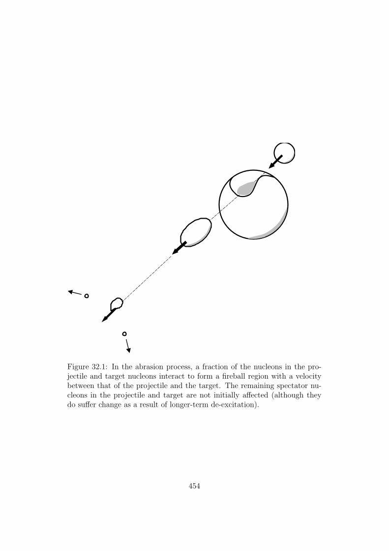
Figure 32.1: In the abrasion process, a fraction of the nucleons in the pro-jectile and target nucleons interact to form a fireball region with a velocitybetween that of the projectile and the target. The remaining spectator nu-cleons in the projectile and target are not initially affected (although theydo suffer change as a result of longer-term de-excitation).

454

Figure 32.2: Illustration clarifying impact parameter in the far-field (b) andactual impact parameter (r).

455

Chapter 33

Electromagnetic DissociationModel

33.1 The Model

The relative motion of a projectile nucleus travelling at relativistic speedswith respect to another nucleus can give rise to an increasingly hard spec-trum of virtual photons. The excitation energy associated with this en-ergy exchange can result in the liberation of nucleons or heavier nuclei (i.e.deuterons, α-particles, etc.). The contribution of this source to the totalinelastic cross section can be important, especially where the proton numberof the nucleus is large. The electromagnetic dissociation (ED) model is im-plemented in the classes G4EMDissociation, G4EMDissociationCrossSectionand G4EMDissociationSpectrum, with the theory taken from Wilson et al[1], and Bertulani and Baur [2].The number of virtual photons N(Eγ, b) per unit area and energy intervalexperienced by the projectile due to the dipole field of the target is given bythe expression [2]:

N (Eγ, b) =αZ2

T

π2β2b2Eγ

x2k21(x) +

(

x2

γ2

)

k20(x)

(33.1)

where x is a dimensionless quantity defined as:

x =bEγ

γβhc(33.2)

and:α = fine structure constantβ = ratio of the velocity of the projectile in the laboratory frame to

the velocity of light

456

γ = Lorentz factor for the projectile in the laboratory frameb = impact parameterc = speed of lighth = quantum constantEγ = energy of virtual photonk0 and k1 = zeroth and first order modified Bessel functions of the

second kindZT = atomic number of the target nucleus

Integrating Eq. 33.1 over the impact parameter from bmin to ∞ producesthe virtual photon spectrum for the dipole field of:

NE1 (Eγ) =2αZ2

T

πβ2Eγ

ξk0(ξ)k1(ξ)−ξ2β2

2

(

k21(ξ)− k20(ξ))

(33.3)

where, according to the algorithm implemented by Wilson et al in NUCFRG2[1]:

ξ = Eγbmin

γβhc

bmin = (1 + xd)bc +πα0

2γ

α0 =ZPZT e2

µβ2c2

bc = 1.34

[

A1/3P + A

1/3T − 0.75

(

A−1/3P + A

−1/3T

)]

(33.4)

and µ is the reduced mass of the projectile/target system, xd = 0.25, and AP

and AT are the projectile and target nucleon numbers. For the last equation,the units of bc are fm. Wilson et al state that there is an equivalent virtualphoton spectrum as a result of the quadrupole field:

NE2 (Eγ) =2αZ2

T

πβ4Eγ

2(

1− β2)

k21(ξ) + ξ(

2− β2)2k0(ξ)k1(ξ)−

ξ2β4

2

(

k21(ξ)− k20(ξ))

(33.5)The cross section for the interaction of the dipole and quadrupole fields isgiven by:

σED =

∫

NE1 (Eγ) σE1 (Eγ) dEγ +

∫

NE2 (Eγ) σE2 (Eγ) dEγ (33.6)

457

Wilson et al assume that σE1(Eγ) and σE2(Eγ) are sharply peaked at thegiant dipole and quadrupole resonance energies:

EGDR = hc[

m∗c2R20

8J

(

1 + u− 1+ε+3u1+ε+u

ε)

]− 12

EGQR = 63

A1/3

P

(33.7)

so that the terms for NE1 and NE2 can be taken out of the integrals in Eq.33.6 and evaluated at the resonances.In Eq. 33.7:

u = 3JQ′A

−1/3P

R0 = r0A1/3P

(33.8)

ǫ = 0.0768, Q′ = 17MeV, J = 36.8MeV, r0 = 1.18fm, and m∗ is 7/10 ofthe nucleon mass (taken as 938.95 MeV/c2). (The dipole and quadrupoleenergies are expressed in units of MeV.)The photonuclear cross sections for the dipole and quadrupole resonances areassumed to be given by:

∫

σE1 (Eγ) dEγ = 60NPZP

AP

(33.9)

in units of MeV-mb (NP being the number of neutrons in the projectile) and:

∫

σE2 (Eγ)dEγ

E2γ

= 0.22fZPA2/3P (33.10)

in units of µb/MeV. In the latter expression, f is given by:

f =

0.9 AP > 1000.6 40 < AP ≤ 1000.3 40 ≤ AP

(33.11)

The total cross section for electromagnetic dissociation is therefore given byEq. 33.6 with the virtual photon spectra for the dipole and quadrupole fieldscalculated at the resonances:

458

σED = NE1 (EGDR)

∫

σE1 (Eγ) dEγ +NE2 (EGQR)E2GQR

∫

σE2 (Eγ)

E2γ

dEγ

(33.12)where the resonance energies are given by Eq. 33.7 and the integrals for thephotonuclear cross sections given by Eq. 33.9 and Eq. 33.10.The selection of proton or neutron emission is made according to the followingprescription from Wilson et al.

σED,p = σED ×

0.5 ZP < 60.6 6 ≤ ZP ≤ 80.7 8 < ZP < 14

min[

ZP

AP, 1.95 exp(−0.075ZP )

]

ZP ≥ 14

σED,n = σED − σED,p

(33.13)Note that this implementation of ED interactions only treats the ejection

of single nucleons from the nucleus, and currently does not allow emission ofother light nuclear fragments.

Bibliography

[1] J. W. Wilson, R. K. Tripathi, F. A. Cucinotta, J. K. Shinn, F. F. Badavi,S. Y. Chun, J. W. Norbury, C. J. Zeitlin, L. Heilbronn, and J. Miller,”NUCFRG2: An evaluation of the semiempirical nuclear fragmentationdatabase,” NASA Technical Paper 3533, 1995.

[2] C. A. Bertulani, and G. Baur, Electromagnetic processes in relativisticheavy ion collisions, Nucl Phys, A458, 725-744, 1986.

459

Chapter 34

Precompound model.

34.1 Reaction initial state.

The GEANT4 precompound model is considered as an extension of thehadron kinetic model. It gives a possibility to extend the low energy rangeof the hadron kinetic model for nucleon-nucleus inelastic collision and it pro-vides a ”smooth” transition from kinetic stage of reaction described by thehadron kinetic model to the equilibrium stage of reaction described by theequilibrium deexcitation models.

The initial information for calculation of pre-compound nuclear stageconsists from the atomic mass number A, charge Z of residual nucleus, itsfour momentum P0, excitation energy U and number of excitons n equalsthe sum of number of particles p (from them pZ are charged) and number ofholes h.

At the preequilibrium stage of reaction, we following the [1] approach,take into account all possible nuclear transition the number of excitons nwith ∆n = +2,−2, 0 [1], which defined by transition probabilities. Onlyemmision of neutrons, protons, deutrons, thritium and helium nuclei aretaken into account.

34.2 Simulation of pre-compound reaction

The precompound stage of nuclear reaction is considered until nuclearsystem is not an equilibrium state. Further emission of nuclear fragments orphotons from excited nucleus is simulated using an equilibrium model (seeChapter 35.6).

460

34.2.1 Statistical equilibrium condition

In the state of statistical equilibrium, which is characterized by an eqilib-rium number of excitons neq, all three type of transitions are equiprobable.Thus neq is fixed by ω+2(neq, U) = ω−2(neq, U). From this condition we canget

neq =√

2gU. (34.1)

34.2.2 Level density of excited (n-exciton) states

To obtain Eq. (34.1) it was assumed an equidistant scheme of single-particle levels with the density g ≈ 0.595aA, where a is the level densityparameter, when we have the level density of the n-exciton state as

ρn(U) =g(gU)n−1

p!h!(n− 1)!. (34.2)

34.2.3 Transition probabilities

The partial transition probabilities changing the exciton number by ∆n isdetermined by the squared matrix element averaged over allowed transitions< |M |2 > and the density of final states ρ∆n(n, U), which are really accessiblein this transition. It can be defined as following:

ω∆n(n, U) =2π

h< |M |2 > ρ∆n(n, U). (34.3)

The density of final states ρ∆n(n, U) were derived in paper [2] using the Eq.(34.2) for the level density of the n-exciton state and later corrected for thePauli principle and indistinguishability of identical excitons in paper [3]:

ρ∆n=+2(n, U) =1

2g[gU − F (p+ 1, h+ 1)]2

n+ 1[gU − F (p+ 1, h+ 1)

gU − F (p, h)]n−1,

(34.4)

ρ∆n=0(n, U) =1

2g[gU − F (p, h)]

n[p(p− 1) + 4ph+ h(h− 1)] (34.5)

and

ρ∆n=−2(n, U) =1

2gph(n− 2), (34.6)

where F (p, h) = (p2 + h2 + p− h)/4− h/2 and it was taken to be equal zero.To avoid calculation of the averaged squared matrix element < |M |2 > itwas assumed [1] that transition probability ω∆n=+2(n, U) is the same as the

461

probability for quasi-free scattering of a nucleon above the Fermi level on anucleon of the target nucleus, i. e.

ω∆n=+2(n, U) =< σ(vrel)vrel >

Vint. (34.7)

In Eq. (34.7) the interaction volume is estimated as Vint =43π(2rc + λ/2π)3,

with the De Broglie wave length λ/2π corresponding to the relative velocity< vrel >=

√

2Trel/m, where m is nucleon mass and rc = 0.6 fm.The averaging in < σ(vrel)vrel > is further simplified by

< σ(vrel)vrel >=< σ(vrel) >< vrel > . (34.8)

For σ(vrel) we take approximation:

σ(vrel) = 0.5[σpp(vrel) + σpn(vrel]P (TF/Trel), (34.9)

where factor P (TF/Trel) was introduced to take into account the Pauli prin-ciple. It is given by

P (TF/Trel) = 1− 7

5

TFTrel

(34.10)

for TF

Trel≤ 0.5 and

P (TF/Trel) = 1− 7

5

TFTrel

+2

5

TFTrel

(2− TrelTF

)5/2 (34.11)

for TF

Trel> 0.5.

The free-particle proton-proton σpp(vrel) and proton-neutron σpn(vrel) in-teraction cross sections are estimated using the equations [4]:

σpp(vrel) =10.63

v2rel− 29.93

vrel+ 42.9 (34.12)

and

σpn(vrel) =34.10

v2rel− 82.2

vrel+ 82.2, (34.13)

where cross sections are given in mbarn.The mean relative kinetic energy Trel is needed to calculate < vrel >

and the factor P (TF/Trel) was computed as Trel = Tp + Tn, where meankinetic energies of projectile nucleons Tp = TF + U/n and target nucleonsTN = 3TF/5, respecively.

462

Combining Eqs. (34.3) - (34.7) and assuming that < |M |2 > are the samefor transitions with ∆n = 0 and ∆n = ±2 we obtain for another transitionprobabilities:

ω∆n=0(n, U) =

= <σ(vrel)vrel>Vint

n+1n[ gU−F (p,h)gU−F (p+1,h+1)

]n+1 p(p−1)+4ph+h(h−1)gU−F (p,h)

(34.14)

andω∆n=−2(n, U) =

= <σ(vrel)vrel>Vint

[ gU−F (p,h)gU−F (p+1,h+1)

]n+1 ph(n+1)(n−2)[gU−F (p,h)]2

.(34.15)

34.2.4 Emission probabilities for nucleons

Emission process probability has been choosen similar as in the classicalequilibrium Weisskopf-Ewing model [5]. Probability to emit nucleon b in theenergy interval (Tb, Tb + dTb) is given

Wb(n, U, Tb) = σb(Tb)(2sb + 1)µb

π2h3Rb(p, h)

ρn−b(E∗)

ρn(U)Tb, (34.16)

where σb(Tb) is the inverse (absorption of nucleon b) reaction cross section,sb and mb are nucleon spin and reduced mass, the factor Rb(p, h) takes intoaccount the condition for the exciton to be a proton or neutron, ρn−b(E

∗)and ρn(U) are level densities of nucleus after and before nucleon emission aredefined in the evaporation model, respectively and E∗ = U −Qb − Tb is theexcitation energy of nucleus after fragment emission.

34.2.5 Emission probabilities for complex fragments

It was assumed [1] that nucleons inside excited nucleus are able to ”con-dense” forming complex fragment. The ”condensation” probability to createfragment consisting from Nb nucleons inside nucleus with A nucleons is givenby

γNb= N3

b (Vb/V )Nb−1 = N3b (Nb/A)

Nb−1, (34.17)

where Vb and V are fragment b and nucleus volumes, respectively. The lastequation was estimated [1] as the overlap integral of (constant inside a vol-ume) wave function of independent nucleons with that of the fragment.

During the prequilibrium stage a ”condense” fragment can be emitted.The probability to emit a fragment can be written as [1]

Wb(n, U, Tb) = γNbRb(p, h)

ρ(Nb, 0, Tb +Qb)

gb(Tb)σb(Tb)

(2sb + 1)µb

π2h3ρn−b(E

∗)

ρn(U)Tb,

(34.18)

463

where

gb(Tb) =Vb(2sb + 1)(2µb)

3/2

4π2h3(Tb +Qb)

1/2 (34.19)

is the single-particle density for complex fragment b, which is obtained byassuming that complex fragment moves inside volume Vb in the uniform po-tential well whose depth is equal to be Qb, and the factor Rb(p, h) garanteescorrect isotopic composition of a fragment b.

34.2.6 The total probability

This probability is defined as

Wtot(n, U) =∑

∆n=+2,0,−2

ω∆n(n, U) +6∑

b=1

Wb(n, U), (34.20)

where total emission Wb(n, U) probabilities to emit fragment b can be ob-tained from Eqs. (34.16) and (34.18) by integration over Tb:

Wb(n, U) =

∫ U−Qb

Vb

Wb(n, U, Tb)dTb. (34.21)

34.2.7 Calculation of kinetic energies for emitted par-ticle

The equations (34.16) and (34.18) are used to sample kinetic energies ofemitted fragment.

34.2.8 Parameters of residual nucleus.

After fragment emission we update parameter of decaying nucleus:

Af = A− Ab;Zf = Z − Zb;Pf = P0 − pb;

E∗f =

√

E2f − ~P 2

f −M(Af , Zf ).(34.22)

Here pb is the evaporated fragment four momentum.

Bibliography

[1] K.K. Gudima, S.G. Mashnik, V.D. Toneev, Nucl. Phys. A401 329(1983).

464

[2] F. C. Williams, Phys. Lett. B31 180 (1970).

[3] I. Ribansky, P. Oblozinsky, E. Betak, Nucl. Phys. A205 545 (1973).

[4] N. Metropolis et al., Phys. Rev. 100 185 (1958).

[5] V.E. Weisskopf, D.H. Ewing, Phys. Rev. 57 472 (1940).

465

Chapter 35

Evaporation Model

35.1 Introduction

At the end of the pre-equilibrium stage, or a thermalizing process, theresidual nucleus is supposed to be left in an equilibrium state, in which theexcitation energy E∗ is shared by a large number of nucleons. Such an equili-brated compound nucleus is characterized by its mass, charge and excitationenergy with no further memory of the steps which led to its formation. If theexcitation energy is higher than the separation energy, it can still eject nu-cleons and fragments (d, t, 3He, α, others). These constitute the low energyand most abundant part of the emitted particles in the rest system of theresidual nucleus. The emission of particles by an excited compound nucleushas been successfully described by comparing the nucleus with the evapora-tion of molecules from a fluid [1]. The first statistical theory of compoundnuclear decay is due to Weisskopf and Ewing[2].

35.2 Evaporation model

The Weisskopf treatment is an application of the detailed balance principlethat relates the probabilities to go from a state i to another d and viceversathrough the density of states in the two systems:

Pi→dρ(i) = Pd→iρ(d) (35.1)

where Pd→i is the probability per unit of time of a nucleus d captures a particlej and form a compound nucleus i which is proportional to the compoundnucleus cross section σinv. Thus, the probability that a parent nucleus i withan excitation energy E∗ emits a particle j in its ground state with kinetic

466

energy ε is

Pj(ε)dε = gjσinv(ε)ρd(Emax − ε)

ρi(E∗)εdε (35.2)

where ρi(E∗) is the level density of the evaporating nucleus, ρd(Emax−ε) that

of the daugther (residual) nucleus after emission of a fragment j and Emax isthe maximum energy that can be carried by the ejectile. With the spin sj andthe mass mj of the emitted particle, gj is expressed as gj = (2sj+1)mj/π

2~2.

This formula must be implemented with a suitable form for the level den-sity and inverse reaction cross section. We have followed, like many otherimplementations, the original work of Dostrovsky et al. [3] (which representsthe first Monte Carlo code for the evaporation process) with slight modifi-cations. The advantage of the Dostrovsky model is that it leds to a simpleexpression for equation 35.2 that can be analytically integrated and used forMonte Carlo sampling.

35.2.1 Cross sections for inverse reactions

The cross section for inverse reaction is expressed by means of empiricalequation [3]

σinv(ε) = σgα

(

1 +β

ε

)

(35.3)

where σg = πR2 is the geometric cross section.

In the case of neutrons, α = 0.76+ 2.2A− 13 and β = (2.12A− 2

3 − 0.050)/αMeV. This equation gives a good agreement to those calculated from con-tinuum theory [4] for intermediate nuclei down to ε ∼ 0.05 MeV. For lowerenergies σinv,n(ε) tends toward infinity, but this causes no difficulty becauseonly the product σinv,n(ε)ε enters in equation 35.2. It should be noted, thatthe inverse cross section needed in 35.2 is that between a neutron of kineticenergy ε and a nucleus in an excited state.

For charged particles (p, d, t, 3He and α), α = (1 + cj) and β = −Vj ,where cj is a set of parameters calculated by Shapiro [5] in order to providea good fit to the continuum theory [4] cross sections and Vj is the Coulombbarrier.

35.2.2 Coulomb barriers

Coulomb repulsion, as calculated from elementary electrostatics are notdirectly applicable to the computation of reaction barriers but must be cor-rected in several ways. The first correction is for the quantum mechanical

467

phenomenoon of barrier penetration. The proper quantum mechanical ex-pressions for barrier penetration are far too complex to be used if one wishesto retain equation 35.2 in an integrable form. This can be approximatelytaken into account by multiplying the electrostatic Coulomb barrier by acoefficient kj designed to reproduce the barrier penetration approximatelywhose values are tabulated [5].

Vj = kjZjZde

2

Rc

(35.4)

The second correction is for the separation of the centers of the nuclei atcontact, Rc. We have computed this separation as Rc = Rj + Rd where

Rj,d = rcA1/3j,d and rc is given [6] by

rc = 2.1731 + 0.006103ZjZd

1 + 0.009443ZjZd

(35.5)

35.2.3 Level densities

The simplest and most widely used level density based on the Fermigas model are those of Weisskopf [7] for a completely degenerate Fermi gas.We use this approach with the corrections for nucleon pairing proposed byHurwitz and Bethe [8] which takes into account the displacements of theground state:

ρ(E) = C exp(

2√

a(E − δ))

(35.6)

where C is considered as constant and does not need to be specified sinceonly ratios of level densities enter in equation 35.2. δ is the pairing energycorrection of the daughter nucleus evaluated by Cook et al. [9] and Gilbertand Cameron [10] for those values not evaluated by Cook et al.. The leveldensity parameter is calculated according to:

a(E,A, Z) = a(A)

1 +δ

E[1− exp(−γE)]

(35.7)

and the parameters calculated by Iljinov et al. [11] and shell corrections ofTruran, Cameron and Hilf [12].

35.2.4 Maximum energy available for evaporation

The maximum energy avilable for the evaporation process (i.e. themaximum kinetic energy of the outgoing fragment) is usually computedlike E∗ − δ − Qj where is the separation energy of the fragment j: Qj =

468

Mi −Md −Mj and Mi, Md and Mj are the nclear masses of the compound,residual and evporated nuclei respectively. However, that expression doesnot consider the recoil energy of the residual nucleus. In order to take intoaccount the recoil energy we use the expression

εmaxj =

(Mi + E∗ − δ)2 +M2j −M2

d

2(Mi + E∗ − δ)−Mj (35.8)

35.2.5 Total decay width

The total decay width for evaporation of a fragment j can be obtained byintegrating equation 35.2 over kinetic energy

Γj = ~

∫ εmaxj

Vj

P (εj)dεj (35.9)

This integration can be performed analiticaly if we use equation 35.6 for leveldensities and equation 35.3 for inverse reaction cross section. Thus, the totalwidth is given by

Γj =gjmjR

2d

2π~2α

a2d×

(

βad −3

2

)

+ ad(εmaxj − Vj)

exp

−√

ai(E∗ − δi)

+

(2βad − 3)√

ad(εmaxj − Vj) + 2ad(ε

maxj − Vj)

×

exp

2[√

ad(εmaxj − Vj)−

√

ai(E∗ − δi)]

(35.10)

where ad = a(Ad, Zd, εmaxj ) and ai = a(Ai, Zi, E

∗).

35.3 GEM model

As an alternative model we have implemented the generalized evaporationmodel (GEM) by Furihata [13]. This model considers emission of fragmentsheavier than α particles and uses a more accurate level density function fortotal decay width instead of the approximation used by Dostrovsky. We usethe same set of parameters but for heavy ejectiles the parameters determinedby Matsuse et al. [14] are used.

Based on the Fermi gas model, the level density function is expressed as

ρ(E) =

√π

12e2√

a(E−δ)

a1/4(E−δ)5/4for E ≥ Ex

1Te(E−E0)/T for E < Ex

(35.11)

469

where Ex = Ux + δ and Ux = 150/Md + 2.5 (Md is the mass of the daughternucleus). Nuclear temperature T is given as 1/T =

√

a/Ux − 1.5Ux, and E0

is defined as E0 = Ex − T (log T − log a/4− (5/4) logUx + 2√aUx).

By substituting equation 35.11 into equation 35.2 and integrating overkinetic energy can be obtained the following expression

Γj =

√πgjπR

2dα

12ρ(E∗)×

I1(t, t) + (β + V )I0(t) for εmaxj − Vj < Ex

I1(t, tx) + I3(s, sx)es+

(β + V )(I0(tx) + I2(s, sx)es) for εmax

j − Vj ≥ Ex.(35.12)

I0(t), I1(t, tx), I2(s, sx), and I3(s, sx) are expressed as:

I0(t) = e−E0/T (et − 1) (35.13)

I1(t, tx) = e−E0/TT(t− tx + 1)etx − t− 1 (35.14)

I2(s, sx) = 2√2

s−3/2 + 1.5s−5/2 + 3.75s−7/2 −

(s−3/2x + 1.5s−5/2

x + 3.75s−7/2x )

(35.15)

I3(s, sx) =1

2√2

[

2s−1/2 + 4s−3/2 + 13.5s−5/2 + 60.0s−7/2 +

325.125s−9/2 −

(s2 − s2x)s−3/2x + (1.5s2 + 0.5s2x)s

−5/2x +

(3.75s2 + 0.25s2x)s−7/2x + (12.875s2 + 0.625s2x)s

−9/2x +

(59.0625s2 + 0.9375s2x)s−11/2x +

(324.8s2 + 3.28s2x)s−13/2x +

]

(35.16)

where t = (εmaxj − Vj)/T , tx = Ex/T , s = 2

√

a(εmaxj − Vj − δj) and sx =

2√

a(Ex − δ).Besides light fragments, 60 nuclides up to 28Mg are considered, not only in

their ground states but also in their exited states, are considered. The excitedstate is assumed to survive if its lifetime T1/2 is longer than the decay time,i. e., T1/2/ ln 2 > ~/Γ∗

j , where Γ∗j is the emission width of the resonance

calculated in the same manner as for ground state particle emission. Thetotal emission width of an ejectile j is summed over its ground state and allits excited states which satisfy the above condition.

470

35.4 Nuclear fission

The fission decay channel (only for nuclei with A > 65) is taken intoaccount as a competitor for fragment and photon evaporation channels.

35.4.1 The fission total probability

The fission probability (per unit time)Wfis in the Bohr andWheeler theoryof fission [15] is proportional to the level density ρfis(T ) ( approximation Eq.(35.6) is used) at the saddle point, i.e.

Wfis =1

2π~ρfis(E∗)

∫ E∗−Bfis

0ρfis(E

∗ − Bfis − T )dT =

=1+(Cf−1) exp (Cf )

4πafis exp (2√aE∗)

,(35.17)

where Bfis is the fission barrier height. The value of Cf = 2√

afis(E∗ − Bfis)and a, afis are the level density parameters of the compound and of the fissionsaddle point nuclei, respectively.

The value of the level density parameter is large at the saddle point, whenexcitation energy is given by initial excitation energy minus the fission barrierheight, than in the ground state, i. e. afis > a. afis = 1.08a for Z < 85,afis = 1.04a for Z ≥ 89 and af = a[1.04 + 0.01(89.− Z)] for 85 ≤ Z < 89 isused.

35.4.2 The fission barrier

The fission barrier is determined as difference between the saddle-pointand ground state masses.

We use simple semiphenomenological approach was suggested by Barashenkovand Gereghi [16]. In their approach fission barrier Bfis(A,Z) is approximatedby

Bfis = B0fis +∆g +∆p. (35.18)

The fission barrier height B0fis(x) varies with the fissility parameter x =

Z2/A. B0fis(x) is given by

B0fis(x) = 12.5 + 4.7(33.5− x)0.75 (35.19)

for x ≤ 33.5 andB0

fis(x) = 12.5− 2.7(x− 33.5)2/3 (35.20)

for x > 33.5. The ∆g = ∆M(N) +∆M(Z), where ∆M(N) and ∆M(Z) areshell corrections for Cameron’s liquid drop mass formula [17] and the pairingenergy corrections: ∆p = 1 for odd-odd nuclei, ∆p = 0 for odd-even nuclei,∆p = 0.5 for even-odd nuclei and ∆p = −0.5 for even-even nuclei.

471

35.5 Photon evaporation

Photon evaporation main be simulated as a continium gamma transition us-ing dipole approximation and via discrete gamma transition using evaluateddatabase on nuclear gamma transitions.

35.5.1 Computation of probability

As the first approximation we assume that dipole E1–transitions is themain source of γ–quanta from highly–excited nuclei [11]. The probability toevaporate γ in the energy interval (ǫγ, ǫγ + dǫγ) per unit of time is given

Wγ(ǫγ) =1

π2(~c)3σγ(ǫγ)

ρ(E∗ − ǫγ)

ρ(E∗)ǫ2γ , (35.21)

where σγ(ǫγ) is the inverse (absorption of γ) reaction cross section, ρ is anucleus level density is defined by Eq. (35.6).

The photoabsorption reaction cross section is given by the expression

σγ(ǫγ) =σ0ǫ

2γΓ

2R

(ǫ2γ − E2GDP )

2 + Γ2Rǫ

2γ

, (35.22)

where σ0 = 2.5A mb, ΓR = 0.3EGDP and EGDP = 40.3A−1/5 MeV areempirical parameters of the giant dipole resonance [11]. The total radiationprobability is

Wγ =1

π2(~c)3

∫ E∗

0

σγ(ǫγ)ρ(E∗ − ǫγ)

ρ(E∗)ǫ2γdǫγ . (35.23)

The integration is performed numericaly. The energy of γ-quantum is sam-pled according to the Eq. (35.21) distribution.

35.5.2 Discrete photon evaporation

The last step of evaporation cascade consists of evaporation of photonswith discrete energies. The competition between photons and fragments aswell as giant resonance photons is neglected at this step. We consider thediscrete E1, M1 and E2 photon transitions from tabulated isotopes. Thereare large number of isotopes [18] with the experimentally measured exitedlevel energies, spins, parities and relative transitions probabilities. This in-formation is uploaded for each excited state in run time when correspondingexcited state first created.

The list of isotopes included in the photon evaporation data base has beenextended from A <= 240 to A <= 250. The highest atomic number includedis Z = 98 (this ensures that Americium sources can now be simulated).

472

35.5.3 Internal conversion electron emission

An important conpetitive channel to photon emission is internal con-version. To take this into account, the photon evaporation data-base wasentended to include internal conversion coeffficients.

The above constitute the first six columns of data in the photon evap-oration files. The new version of the data base adds eleven new columnscorresponding to:

7. ratio of internal conversion to gamma-ray emmission probability

8. - 17. internal conversion coefficients for shells K, L1, L2, L3, M1, M2,M3, M4, M5 and N+ respectively. These coefficients are normalised to1.0

The calculation of the Internal Conversion Coefficients (ICCs) is done by acubic spline interpolation of tabulalted data for the corresponding transitionenergy. These ICC tables, which we shall label Band [19], Rosel [20] andHager-Seltzer [21], are widely used and were provided in electronic formatby staff at LBNL. The reliability of these tabulated data has been reviewedin Ref. [22]. From tests carried out on these data we find that the ICCscalculated from all three tables are comparable within a 10% uncertainty,which is better than what experimetal measurements are reported to be ableto achive.

The range in atomic number covered by these tables is Band: 1 <= Z <=80; Rosel: 30 <= Z <= 104 and Hager-Seltzer: 3, 6, 10, 14 <= Z <= 103.For simplicity and taking into account the completeness of the tables, wehave used the Band table for Z <= 80 and Rosel for 81 <= Z <= 98.

The Band table provides a higher resolution of the ICC curves used in theinterpolation and covers ten multipolarities for all elements up to Z = 80,but it only includes ICCs for shells up to M5. In order to calculate theICC of the N+ shell, the ICCs of all available M shells are added togetherand the total divided by 3. This is the scheme adopted in the LBNL ICCcalculation code when using the Band table. The Rosel table includes ICCsfor all shells in every atom and for Z > 80 the N+ shell ICC is calculatedby adding together the ICCs of all shells above M5. In this table only eightmultipolarities have ICCs calculated for.

For the production of an internal conversion electron, the energy of thetransition must be at least the binding energy of the shell the electron isbeing released from. The binding energy corresponding to the various shellsin all isotopes used in the ICC calculation has been taken from the Geant4file G4AtomicShells.hh.

473

The ENSDF data provides information on the multipolarity of the tran-sition. The ICCs included in the photon evaporation data base refer to themultipolarity indicated in the ENSDF file for that transition. Only one typeof mixed mulltipolarity is considered (M1+E2) and whenever the mixing ratiois provided in the ENSDF file, it is used to calculate the ICCs correspondingto the mixed multipolarity according the the formula:

- fraction in M1 = 1/(1 + δ2)- fraction in E2 = δ2/(1 + δ2)

where δ is the mixing ratio.

35.6 Sampling procedure

The evaporation model algorithm consists from repeating steps on decaychannels. The stack of excited nuclear fragments is created and initial excitedfragent is stored there. For the each fragment from the stack decay chain issampled via loop of actions:

1. switch to the next excited fragment in the stack;

2. check if Fermi break-up model 37.1 is applicable and apply this modelif it is the case;

3. sort out decay products between store of excited fragments and the listof final products;

4. if Fermi break up is not applicable compute probabilities of all evapo-ration channels;

5. randomly select of a break-up channel and sample final state for theselected channel;

6. sort out decay products between store of excited fragments and the listof final products;

7. check if the residual fragment is stable, stop the loop if it is the caseand store residual fragment to the list of final products;

8. if the fragment is not stable check if Fermi break-up is applicable, if yesthen store this residual into the stack of excited fragments, else repeatfrom (4).

474

Bibliography

[1] I. Frenkel. Sov. Phys. 9 533 (1936).

[2] V. E. Weisskopf and D. H. Ewing. Phys. Rev. 57 472 (1940).

[3] I. Dostrovsky, Z. Fraenkel, G. Friedlander. Phys. Rev. 116 683 (1959).

[4] J. Blatt and V. F. Weisskopf, Theoretical Nuclear Physics (John Wiley& Sons, Inc., New York, 1952)

[5] M. M. Shapiro. Phys. Rev. 90, 171 (1953).

[6] A. S. Iljinov, M. V. Kazarnovsky and E. Ya. Paryev. Intermediate–Energy Nuclear Physics (CRC Press, 1994).

[7] V. F. Weisskopf. Phys. Rev. 52, 295 (1937)

[8] H. Hurwitz and H. A. Bethe. Phys. Rev. 81, (1951)

[9] J.L. Cook, H. Ferguson and A. R. L. Musgrove. Aust. J. Phys., 20, 477(1967)

[10] A. Gilbert and A.G.W. Cameron, Can. J. Phys., 43, 1446 (1965)

[11] A. S. Iljinov, M. V. Mevel et al.. Nucl. Phys. A543, 517 (1992).

[12] J. W. Truran, A. G. W. Cameron, and E. Hilf. Proc. Int. Conf. on theProperties of Nuclei Far From the Beta-Stability Leysin, Switzerland,August 31 - September 4, 1970, Vol.1, p. 275

[13] S. Furihata. Nucl. Instr. and Meth. in Phys. Res. B171, 251 (2000)

[14] T. Matsuse, A. Arima, and S. M. Lee. Phys. Rev. C 26, 2338 (1982)

[15] Bohr N., Wheeler J. W., Phys. Rev., 56 426 (1939).

[16] Barashenkov V. S., Iljinov A. S., Toneev V. D., Gereghi F. G, Nucl.Phys. A206 131 (1973).

[17] Cameron A. G. W. Canad. J. Phys., 35 1021 (1957), 36 1040 (1958).

[18] Evaluated Nuclear Structure Data File (ENSDF) - a computer fileof evaluated experimental nuclear structure data maintained by theNational Nuclear Data Center, Brookhaven National Laboratory(http://www.nndc.bnl.gov/nndc/nudat/).

475

[19] I.M. Band and M.B. Trzhaskovskaya, Tables of the Gamma-ray InternalConversion Coefficients for the K, L, M Shells, for 1 <= Z <= 80,Leningrad: Nuclear Physics Institute (1978).

[20] F. Rosel, H.M. Fries, K. Alder and H.C. Pauli, At. Data Nucl. DataTables 21 (1978).

[21] R.S. Hager and E.C. Seltzer, Nucl. Data A4 (1968).

[22] M. Rysavy and O. Dragoun, On the Reliability of the Theoretical Inter-nal Conversion Coefficients, J. Phys. G: Nucl. Part. Phys., 2000, v.26,N. 12, pp 1859-72.

476

Chapter 36

Fission model.

36.1 Reaction initial state.

The GEANT4 fission model is capable to predict final excited fragmentsas result of an excited nucleus symmetric or asymmetric fission. The fissionprocess (only for nuclei with atomic number A ≥ 65) is considered as a com-petitor for evaporation process, when nucleus transits from an excited stateto the ground state. Here we describe the final state generation. The cal-culation of the relative probability of fission with respect to the evaporationchannels are described in the chapter concerning evaporation.

The initial information for calculation of fission decay consists from theatomic mass number A, charge Z of excited nucleus, its four momentum P0

and excitation energy U .

36.2 Fission process simulation.

36.2.1 Atomic number distribution of fission products.

As follows from experimental data [1] mass distribution of fission productsconsists of the symmetric and the asymmetric components:

F (Af ) = Fsym(Af ) + ωFasym(Af ), (36.1)

where ω(U,A, Z) defines relative contribution of each component and it de-pends from excitation energy U and A,Z of fissioning nucleus. It was foundin [2] that experimental data can be approximated with a good accuracy, ifone take

Fsym(Af ) = exp [−(Af − Asym)2

2σ2sym

] (36.2)

477

andFasym(Af ) = exp [− (Af−A2)2

2σ22

] + exp [−Af−(A−A2)2

2σ22

]+

+Casymexp [− (Af−A1)2

2σ21

] + exp [−Af−(A−A1)2

2σ22

],(36.3)

where Asym = A/2, A1 and A2 are the mean values and σ2sim, σ

21 and σ2

2 aredispertions of the Gaussians respectively. From an analysis of experimentaldata [2] the parameter Casym ≈ 0.5 was defined and the next values fordispersions:

σ2sym = exp (0.00553U + 2.1386), (36.4)

where U in MeV,2σ1 = σ2 = 5.6 MeV (36.5)

for A ≤ 235 and

2σ1 = σ2 = 5.6 + 0.096(A− 235) MeV (36.6)

for A > 235 were found.The weight ω(U,A, Z) was approximated as follows

ω =ωa − Fasym(Asym)

1− ωaFsym((A1 + A2)/2). (36.7)

The values of ωa for nuclei with 96 ≥ Z ≥ 90 were approximated by

ωa(U) = exp (0.538U − 9.9564) (36.8)

for U ≤ 16.25 MeV,

ωa(U) = exp (0.09197U − 2.7003) (36.9)

for U > 16.25 MeV and

ωa(U) = exp (0.09197U − 1.08808) (36.10)

for z = 89. For nuclei with Z ≤ 88 the authors of [2] constracted the followingapproximation:

ωa(U) = exp [0.3(227− a)] exp 0.09197[U − (Bfis − 7.5)]− 1.08808,(36.11)

where for A > 227 and U < Bfis − 7.5 the corresponding factors occuring inexponential functions vanish.

478

36.2.2 Charge distribution of fission products.

At given mass of fragment Af the experimental data [1] on the charge Zf

distribution of fragments are well approximated by Gaussian with dispertionσ2z = 0.36 and the average < Zf > is described by expression:

< Zf >=Af

AZ +∆Z, (36.12)

when parameter ∆Z = −0.45 for Af ≥ 134, ∆Z = −0.45(Af −A/2)/(134−A/2) for A− 134 < Af < 134 and ∆Z = 0.45 for A ≤ A− 134.

After sampling of fragment atomic masses numbers and fragment charges,we have to check that fragment ground state masses do not exceed initialenergy and calculate the maximal fragment kinetic energy

Tmax < U +M(A,Z)−M1(Af1, Zf1)−M2(Af2, Zf2), (36.13)

where U and M(A,Z) are the excitation energy and mass of initial nucleus,M1(Af1, Zf1), and M2(Af2, Zf2) are masses of the first and second fragment,respectively.

36.2.3 Kinetic energy distribution of fission products.

We use the empiricaly defined [3] dependence of the average kinetic energy< Tkin > (in MeV) of fission fragments on the mass and the charge of afissioning nucleus:

< Tkin >= 0.1178Z2/A1/3 + 5.8. (36.14)

This energy is distributed differently in cases of symmetric and asymmetricmodes of fission. It follows from the analysis of data [2] that in the asym-metric mode, the average kinetic energy of fragments is higher than that inthe symmetric one by approximately 12.5 MeV. To approximate the averagenumbers of kinetic energies < T sym

kin and < T asymkin > for the symmetric and

asymmetric modes of fission the authors of [2] suggested empirical expres-sions:

< T symkin >=< Tkin > −12.5Wasim, (36.15)

< T asymkin >=< Tkin > +12.5Wsim, (36.16)

where

Wsim = ω

∫

Fsim(A)dA/

∫

F (A)dA (36.17)

and

Wasim =

∫

Fasim(A)dA/

∫

F (A)dA, (36.18)

479

respectively. In the symmetric fission the experimental data for the ratio ofthe average kinetic energy of fission fragments < Tkin(Af ) > to this maximumenergy < Tmax

kin > as a function of the mass of a larger fragment Amax can beapproximated by expressions

< Tkin(Af ) > / < Tmaxkin >= 1− k[(Af − Amax)/A]

2 (36.19)

for Asim ≤ Af ≤ Amax + 10 and

< Tkin(Af ) > / < Tmaxkin >= 1− k(10/A)2 − 2(10/A)k(Af − Amax − 10)/A

(36.20)for Af > Amax + 10, where Amax = Asim and k = 5.32 and Amax = 134 andk = 23.5 for symmetric and asymmetric fission respectively. For both modesof fission the distribution over the kinetic energy of fragments Tkin is choosenGaussian with their own average values < Tkin(Af ) >=< T sym

kin (Af ) > or< Tkin(Af ) >=< T asym

kin (Af ) > and dispersions σ2kin equal 82 MeV or 102

MeV2 for symmetrical and asymmetrical modes, respectively.

36.2.4 Calculation of the excitation energy of fissionproducts.

The total excitation energy of fragments Ufrag can be defined according toequation:

Ufrag = U +M(A,Z)−M1(Af1, Zf1)−M2(Af2, Zf2)− Tkin, (36.21)

where U and M(A,Z) are the excitation energy and mass of initial nucleus,Tkin is the fragments kinetic energy, M1(Af1, Zf1), and M2(Af2, Zf2) aremasses of the first and second fragment, respectively.

The value of excitation energy of fragment Uf determines the fragmenttemperature (T =

√

Uf/af , where af ∼ Af is the parameter of fragmentlevel density). Assuming that after disintegration fragments have the sametemperature as initial nucleus than the total excitation energy will be dis-tributed between fragments in proportion to their mass numbers one obtains

Uf = UfragAf

A. (36.22)

36.2.5 Excited fragment momenta.

Assuming that fragment kinetic energy Tf = P 2f /(2(M(Af , Zf + Uf ) we

are able to calculate the absolute value of fragment c.m. momentum

Pf =(M1(Af1, Zf1 + Uf1)(M2(Af2, Zf2 + Uf2)

M1(Af1, Zf1) + Uf1 +M2(Af2, Zf2) + Uf2

Tkin. (36.23)

480

and its components, assuming fragment isotropical distribution.

Bibliography

[1] Vandenbosch R., Huizenga J. R., Nuclear Fission, Academic Press,New York, 1973.

[2] Adeev G. D. et al. Preprint INR 816/93, Moscow, 1993.

[3] Viola V. E., Kwiatkowski K. and Walker M, Phys. Rev. C31 1550(1985).

481

Chapter 37

Fermi break-up model.

37.1 Fermi break-up simulation for light nu-

clei

For light nuclei the values of excitation energy per nucleon are oftencomparable with nucleon binding energy. Thus a light excited nucleus breaksinto two or more fragments with branching given by available phase space.To describe a process of nuclear disassembling the so-called Fermi break-up model is formulated [1], [2], [3], [4]. This statistical approach was firstused by Fermi [1] to describe the multiple production in high energy nucleoncollision. The GEANT4 Fermi break-up model is capable to predict finalstates as result of an excited nucleus with Z < 9 and A < 17 statisticalbreak-up.

37.1.1 Allowed channels

The channel will be allowed for decay, if the total kinetic energy Ekin of allfragments of the given channel at the moment of break-up is positive. Thisenergy can be calculated according to equation:

Ekin = U +M(A,Z)− ECoulomb −n∑

b=1

(mb + ǫb), (37.1)

U is primary fragment excitation, mb and ǫb are masses and excitation en-ergies of fragments, respectively, ECoulomb is the Coulomb barrier for a givenchannel. It is approximated by

ECoulomb =3

5

e2

r0(1 +

V

V0)−1/3(

Z2

A1/3−

n∑

b=1

Z2

A1/3b

), (37.2)

482

where V0 is the volume of the system corresponding to the normal nuclearmatter density

V0 = 4πR3/3 = 4πr30A/3, (37.3)

where r0 = 1.3fm is used. Free parameter of the model is the ratio of theeffective volume V to the normal volume, currently

κ =V

V0= 6. (37.4)

37.1.2 Break-up probability

The total probability for nucleus to break-up into n componets (nucleons,deutrons, tritons, alphas etc) in the final state is given by

W (E, n) = (V/Ω)n−1ρn(E), (37.5)

where ρn(E) is the density of a number of final states, Ω = (2π~)3 is thenormalization volume. The density ρn(E) can be defined as a product ofthree factors:

ρn(E) =Mn(E)SnGn. (37.6)

The first one is the phase space factor defined as

Mn =

∫ +∞

−∞...

∫ +∞

−∞δ(

n∑

b=1

pb)δ(E −n∑

b=1

√

p2 +m2b)

n∏

b=1

d3pb, (37.7)

where pb is fragment b momentum. The second one is the spin factor

Sn =n∏

b=1

(2sb + 1), (37.8)

which gives the number of states with different spin orientations. The lastone is the permutation factor

Gn =k∏

j=1

1

nj!, (37.9)

which takes into account identity of components in final state. nj is a number

of components of j- type particles and k is defined by n =∑k

j=1 nj).In non-relativistic case (Eq. (37.11) the integration in Eq. (37.7) can be

evaluated analiticaly (see e. g. [6]). The probability for a nucleus with energy

483

E disassembling into n fragments with masses mb, where b = 1, 2, 3, ..., nequals

W (Ekin, n) = SnGn(V

Ω)n−1(

1∑n

b=1mb

n∏

b=1

mb)3/2 (2π)3(n−1)/2

Γ(3(n− 1)/2)E

3n/2−5/2kin ,

(37.10)where Γ(x) is the gamma function.

37.1.3 Fragment characteristics

We take into account the formation of fragments in their ground and low-lying excited states, which are stable for nucleon emission. However, severalunstable fragments with large lifetimes: 5He, 5Li, 8Be, 9B etc are also consid-ered. Fragment characteristics Ab, Zb, sb and ǫb are taken from [7]. Recentlynuclear level energies were changed to be identical with nuclear levels in thegamma evaporation database (see Chapter 35.5.2).

37.1.4 Sampling procedure

The nucleus break-up is described by the Monte Carlo (MC) procedure.We randomly (according to probability Eq. (37.10) and condition Eq. (37.1))select decay channel. Then for given channel we calculate kinematical quan-tities of each fragment according to n-body phase space distribution:

Mn =

∫ +∞

−∞...

∫ +∞

−∞δ(

n∑

b=1

pb)δ(n∑

b=1

p2b2mb

− Ekin)n∏

b=1

d3pb. (37.11)

The Kopylov’s sampling procedure [8] is applied. The angular distributionsfor emitted fragments are considered to be isotropical.

Bibliography

[1] Fermi E., Prog. Theor. Phys. 5 1570 (1950).

[2] Kretschmar M. Annual Rev. Nucl. Sci. 11 1 (1961).

[3] Epherre M., Gradsztajn E., J. Physique 18 48 (1967).

[4] Bonorf J. P., Botvina A. S., Iljinov A. S., Mishustin I. N., Sneppen K.,Phys. Rep. 257 133 (1995).

[5] Cameron A. G. W. Canad. J. Phys., 35 1021 (1957), 36 1040 (1958).

484

[6] Barashenkov V. S., Barbashov B. M., Bubelev E. G. Nuovo Cimento,7 117 (1958).

[7] Ajzenberg-Selone F., Nucl. Phys. 1 360 (1981); A375 (1982); 392(1983); A413 (1984); A433 (1985).

[8] Kopylov G. I., Principles of resonance kinematics, Moscow, Nauka,1970 (in Russian).

485

Chapter 38

Multifragmentation model.

38.1 Multifragmentation process simulation.

The GEANT4 multifragmentation model is capable to predict final statesas result of an highly excited nucleus statistical break-up.

The initial information for calculation of multifragmentation stage con-sists from the atomic mass number A, charge Z of excited nucleus and itsexcitation energy U . At high excitation energies U/A > 3 MeV the multi-fragmentation mechanism, when nuclear system can eventually breaks downinto fragments, becomes the dominant. Later on the excited primary frag-ments propagate independently in the mutual Coulomb field and undergode-excitation. Detailed description of multifragmentation mechanism andmodel can be found in review [1].

38.1.1 Multifragmentation probability.

The probability of a breakup channel b is given by the expression (in theso-called microcanonical approach [1], [2]):

Wb(U,A, Z) =1

∑

b exp[Sb(U,A, Z)]exp[Sb(U,A, Z)], (38.1)

where Sb(U,A, Z) is the entropy of a multifragment state corresponding to thebreakup channel b. The channels b can be parametrized by set of fragmentmultiplicities NAf ,Zf

for fragment with atomic number Af and charge Zf .All partitions b should satisfy constraints on the total mass and charge:

∑

f

NAf ,ZfAf = A (38.2)

486

and∑

f

NAf ,ZfZf = Z. (38.3)

It is assumed [2] that thermodynamic equilibrium is established in everychannel, which can be characterized by the channel temperature Tb.

The channel temperature Tb is determined by the equation constrainingthe average energy Eb(Tb, V ) associated with partition b:

Eb(Tb, V ) = U + Eground = U +M(A,Z), (38.4)

where V is the system volume, Eground is the ground state (at Tb = 0) energyof system and M(A,Z) is the mass of nucleus.

According to the conventional thermodynamical formulae the average en-ergy of a partitition b is expressed through the system free energy Fb asfollows

Eb(Tb, V ) = Fb(Tb, V ) + TbSb(Tb, V ). (38.5)

Thus, if free energy Fb of a partition b is known, we can find the channeltemperature Tb from Eqs. (38.4) and (38.5), then the entropy Sb = −dFb/dTband hence, decay probability Wb defined by Eq. (38.1) can be calculated.

Calculation of the free energy is based on the use of the liquid-drop de-scription of individual fragments [2]. The free energy of a partition b can besplitted into several terms:

Fb(Tb, V ) =∑

f

Ff (Tb, V ) + EC(V ), (38.6)

where Ff (Tb, V ) is the average energy of an individual fragment includingthe volume

F Vf = [−E0 − T 2

b /ǫ(Af )]Af , (38.7)

surfaceF Surf = β0[(T

2c − T 2

b )/(T2c + T 2

b )]5/4A

2/3f = β(Tb)A

2/3f , (38.8)

symmetryF Simf = γ(Af − 2Zf )

2/Af , (38.9)

Coulomb

FCf =

3

5

Z2fe

2

r0A1/3f

[1− (1 + κC)−1/3] (38.10)

and translational

F tf = −Tb ln (gfVf/λ3Tb

) + Tb ln (NAf ,Zf!)/NAf ,Zf

(38.11)

487

terms and the last term

EC(V ) =3

5

Z2e2

R(38.12)

is the Coulomb energy of the uniformly charged sphere with charge Ze andthe radius R = (3V/4π)1/3 = r0A

1/3(1 + κC)1/3, where κC = 2 [2].

Parameters E0 = 16 MeV, β0 = 18 MeV, γ = 25 MeV are the coefficientsof the Bethe-Weizsacker mass formula at Tb = 0. gf = (2Sf + 1)(2If + 1)is a spin Sf and isospin If degeneracy factor for fragment ( fragments withAf > 1 are treated as the Boltzmann particles), λTb

= (2πh2/mNTb)1/2 is

the thermal wavelength, mN is the nucleon mass, r0 = 1.17 fm, Tc = 18MeV is the critical temperature, which corresponds to the liquid-gas phasetransition. ǫ(Af ) = ǫ0[1 + 3/(Af − 1)] is the inverse level density of themass Af fragment and ǫ0 = 16 MeV is considered as a variable modelparameter, whose value depends on the fraction of energy transferred to theinternal degrees of freedom of fragments [2]. The free volume Vf = κV =κ43πr40A available to the translational motion of fragment, where κ ≈ 1 and

its dependence on the multiplicity of fragments was taken from [2]:

κ = [1 +1.44

r0A1/3(M1/3 − 1)]3 − 1. (38.13)

For M = 1 κ = 0.The light fragments with Af < 4, which have no excited states, are con-

sidered as elementary particles characterized by the empirical masses Mf ,radii Rf , binding energies Bf , spin degeneracy factors gf of ground states.They contribute to the translation free energy and Coulomb energy.

38.1.2 Direct simulation of the low multiplicity multi-fragment disintegration

At comparatively low excitation energy (temperature) system will disin-tegrate into a small number of fragments M ≤ 4 and number of channel isnot huge. For such situation a direct (microcanonical) sorting of all decaychannels can be performed. Then, using Eq. (38.1), the average multiplicityvalue < M > can be found. To check that we really have the situation withthe low excitation energy, the obtained value of < M > is examined to obeythe inequality < M >≤ M0, where M0 = 3.3 and M0 = 2.6 for A ∼ 100and for A ∼ 200, respectively [2]. If the discussed inequality is fulfilled, thenthe set of channels under consideration is belived to be able for a correctdescription of the break up. Then using calculated according Eq. (38.1)probabilities we can randomly select a specific channel with given values ofAf and Zf .

488

38.1.3 Fragment multiplicity distribution.

The individual fragment multiplicities NAf ,Zfin the so-called macrocanon-

ical ensemble [1] are distributed according to the Poisson distribution:

P (NAf ,Zf) = exp (−ωAf ,Zf

)ωNAf ,Zf

Af ,Zf

NAf ,Zf!

(38.14)

with mean value < NAf ,Zf>= ωAf ,Zf

defined as

< NAf ,Zf>= gfA

3/2f

Vfλ3Tb

exp [1

Tb(Ff (Tb, V )− F t

f (Tb, V )− µAf − νZf )],

(38.15)where µ and ν are chemical potentials. The chemical potential are found bysubstituting Eq. (38.15) into the system of constraints:

∑

f

< NAf ,Zf> Af = A (38.16)

and∑

f

< NAf ,Zf> Zf = Z (38.17)

and solving it by iteration.

38.1.4 Atomic number distribution of fragments.

Fragment atomic numbers Af > 1 are also distributed according to thePoisson distribution [1] (see Eq. (38.14)) with mean value < NAf

> definedas

< NAf>= A

3/2f

Vfλ3Tb

exp [1

Tb(Ff (Tb, V )− F t

f (Tf , V )− µAf − ν < Zf >)],

(38.18)where calculating the internal free energy Ff (Tb, V ) − F t

f (Tb, V ) one has tosubstitute Zf →< Zf >. The average charge < Zf > for fragment havingatomic number Af is given by

< Zf (Af ) >=(4γ + ν)Af

8γ + 2[1− (1 + κ)−1/3]A2/3f

. (38.19)

489

38.1.5 Charge distribution of fragments.

At given mass of fragment Af > 1 the charge Zf distribution of fragmentsare described by Gaussian

P (Zf (Af )) ∼ exp [−(Zf (Af )− < Zf (Af ) >)2

2(σZf(Af ))2

] (38.20)

with dispertion

σZf (Af ) =

√

AfTb

8γ + 2[1− (1 + κ)−1/3]A2/3f

≈√

AfTb8γ

. (38.21)

and the average charge < Zf (Af ) > defined by Eq. (38.17).

38.1.6 Kinetic energy distribution of fragments.

It is assumed [2] that at the instant of the nucleus break-up the kineticenergy of the fragment T f

kin in the rest of nucleus obeys the Boltzmann dis-tribution at given temperature Tb:

dP (T fkin)

dT fkin

∼√

T fkin exp (−T f

kin/Tb). (38.22)

Under assumption of thermodynamic equilibrium the fragment have isotropicvelocities distribution in the rest frame of nucleus. The total kinetic energyof fragments should be equal 3

2MTb, where M is fragment multiplicity, and

the total fragment momentum should be equal zero. These conditions arefullfilled by choosing properly the momenta of two last fragments.

The initial conditions for the divergence of the fragment system are de-termined by random selection of fragment coordinates distributed with equalprobabilities over the break-up volume Vf = κV . It can be a sphere or pro-longated ellipsoid. Then Newton’s equations of motion are solved for allfragments in the self-consistent time-dependent Coulomb field [2]. Thus theasymptotic energies of fragments determined as result of this procedure differfrom the initial values by the Coulomb repulsion energy.

38.1.7 Calculation of the fragment excitation energies.

The temparature Tb determines the average excitation energy of each frag-ment:

Uf (Tb) = Ef (Tb)− Ef (0) =T 2b

ǫ0Af + [β(Tb)− Tb

dβ(Tb)

dTb− β0]A

2/3f , (38.23)

490

where Ef (Tb) is the average fragment energy at given temperature Tb andβ(Tb) is defined in Eq. (38.8). There is no excitation for fragment withAf < 4, for 4He excitation energy was taken as U4He = 4T 2

b /ǫo.

Bibliography

[1] Bondorf J. P., Botvina A. S., Iljinov A. S., Mishustin I. N., SneppenK., Phys. Rep. 257 133 (1995).

[2] Botvina A. S. et al., Nucl. Phys. A475 663 (1987).

491

Chapter 39

INCL++: the Liege IntranuclearCascade model

39.1 Introduction

There is a renewed interest in the study of spallation reactions. This is largelydue to new technological applications, such as Accelerator-Driven Systems,consisting of sub-critical nuclear reactor coupled to a particle accelerator.These applications require optimized targets as spallation sources. This typeof problem typically involves a large number of parameters and thus it cannotbe solved by trial and error. One has to rely on simulations, which impliesthat very accurate tools need to be developed and their validity and accuracyneed to be assessed.

Above ∼200 MeV incident energy it is necessary to use reliable mod-els due to the prohibitive number of open channels. The most appropriatemodeling technique in this energy region is intranuclear cascade (INC) com-bined with evaporation model. One such pair of models is the Liege cascademodel INCL++ [1, 2] coupled with the G4ExcitationHandler statistical de-excitation model. The strategy adopted by the INCL++ cascade is to improvethe quasi-classical treatment of physics without relying on too many freeparameters.

This chapter introduces the physics provided by INCL++ as implementedin Geant4. Table 39.1 summarizes the key features and provides referencesto detailed descriptions of the physics.

The INCL++ model is available through dedicated physics lists (see Ta-ble 39.1). The * HP variants of the physics lists use the NeutronHP model(Chapter 41) for neutron interactions at low energy; the QGSP * and FTFP *

variants respectively use the QGSP and FTFPmodel at high energy. Figure 39.1

492

1.5 AMeV

3 AGeV

10 AGeV

20 AMeV

Figure 39.1: Model map for the INCL++-based physics lists. The first twocolumns represent nucleon- and pion-induced reactions. The third columnrepresents nucleus-nucleus reactions where at least one of the partners isbelow A = 18. The fourth column represents other nucleus-nucleus reactions.

shows a schematic model map of the INCL++-based physics lists.Finally, the INCL++ model is directly accessible through its interface

(G4INCLXXInterface).The reference paper for the INCL++ model is Ref. [2]. Please make sure

you cite it appropriately if you publish any work based on this model.

39.1.1 Suitable application fields

The INCL++-dedicated physics lists are suitable for the simulation of anysystem where spallation reactions or light-ion-induced reactions play a dom-inant role. As examples, we include here a non-exhaustive list of possibleapplication fields:

• Accelerator-Driven Systems (ADS);

• spallation targets;

• radioprotection close to high-energy accelerators;

493

• radioprotection in space;

• proton or carbon therapy;

• production of beams of exotic nuclei.

39.2 Generalities of the INCL++ cascade

INCL++ is a Monte-Carlo simulation incorporating the aforementioned cas-cade physics principles. The INCL++ algorithm consists of an initializationstage and the actual data processing stage.

The INCL++ cascade can be used to simulate the collisions between bulletparticles and nuclei. The supported bullet particles and the interface classessupporting them are presented in table 39.1.

The momenta and positions of the nucleons inside the nuclei are deter-mined at the beginning of the simulation run by modeling the nucleus as afree Fermi gas in a static potential well with a realistic density. The cascadeis modeled by tracking the nucleons and their collisions.

The possible reactions inside the nucleus are

• NN → NN (elastic scattering)

• NN → N∆ and N∆ → NN

• ∆ → πN and πN → ∆

• NN → NN xπ (multiple pion production)

• πN → πN (elastic scattering and charge exchange)

• πN → N (x+ 1)π (multiple pion production)

39.2.1 Model limits

The INCL++ model has certain limitations with respect to the bullet particleenergy and type, and target-nucleus type. The supported energy range forincident nucleons and pions is 1 MeV–20 GeV. Any target nucleus fromdeuterium (2H) up is in principle acceptable, but not all areas of the nuclidechart have received equal attention during testing. Heavy nuclei (say aboveFe) close to the stability valley have been more thoroughly studied than lightor unstable nuclei. The model is anyway expected to accept any existingnucleus as a target.

494

Light nuclei (from A = 2 to A = 18 included) can also be used as pro-jectiles. The G4INCLXXInterface class can be used for collisions betweennuclei of any mass, but it will internally rely on the Binary Cascade model(see chapter 30) if both reaction partners have A > 18. A warning messagewill be displayed (once) if this happens.

39.3 Physics ingredients

The philosophy of the INCL++ model is to minimize the number of free pa-rameters, which guarantees the predictive power of the model. All INCL++parameters are either taken from known phenomenology (e.g. nuclear radii,elementary cross sections, nucleon potentials) or fixed once and for all (stop-ping time, cluster-coalescence parameters).

The nucleons are modeled as a free Fermi gas in a static potential well.The radius of the well depends on the nucleon momentum, the r-p correlationbeing determined by the desired spatial density distribution ρr(r) accordingto the following equation:

ρp(p)p2dp = −dρr(r)

dr

r3

3dr, (39.1)

where ρp(p) is the momentum-space density (a hard-sphere of radius equalto the Fermi momentum).

After the initialization a projectile particle, or bullet, is shot towards thetarget nucleus. In the following we assume that the projectile is a nucleonor a pion; the special case of composite projectiles will be described in moredetail in subsection 39.3.4.

The impact parameter, i.e. the distance between the projectile particleand the center point of the projected nucleus surface is chosen at random.The value of the impact parameter determines the point where the bulletparticle will enter the calculation volume. After this the algorithm tracksthe nucleons by determining the times at which an event will happen. Thepossible events are:

• collision

• decay of a delta resonance

• reflection from the nuclear potential well

• transmission through the nuclear potential well

495

The particles are assumed to propagate along straight-line trajectories.The algorithm calculates the time at which events will happen and propagatesthe particles directly to their positions at that particular point in time. Thismeans that the length of the time step in simulation is not constant, and thatwe do not need to perform expensive numerical integration of the particletrajectories.

Particles in the model are labeled either as participants (projectile parti-cles and particles that have undergone a collision with a projectile) or spec-tators (target particles that have not undergone any collision). Collisionsbetween spectator particles are neglected.

39.3.1 Emission of composite particles

INCL++ is able to simulate the emission of composite particles (up to A = 8)during the cascade stage. Clusters are formed by coalescence of nucleons;when a nucleon (the leading particle) reaches the surface and is about toleave the system, the coalescence algorithm looks for other nucleons that are“sufficiently close” in phase space; if any are found, a candidate cluster isformed. If several clusters are formed, the algorithm selects the least excitedone. Penetration of the Coulomb barrier is tested for the candidate cluster,which is emitted if the test is successful; otherwise, normal transmission ofthe leading nucleon is attempted.

There are at least two peculiarities of INCL++’s cluster-coalescence algo-rithm. First, it acts in phase space, while many existing algorithms act inmomentum space only. Second, it is dynamical, in the sense that it acts onthe instantaneous phase-space distribution of nucleons in the system, andnot on the distribution of the escaping nucleons.

39.3.2 Cascade stopping time

Stopping time is defined as the point in time when the cascade phase isfinished and the excited remnant is passed to evaporation model. In theINCL++ model the stopping time, tstop, is defined as:

tstop = t0(Atarget/208)0.16. (39.2)

Here Atarget is the target mass number and t0 = 70 fm/c. The intranuclearcascade also stops if no participants are left in the nucleus.

496

39.3.3 Conservation laws

The INCL++ model generally guarantees energy and momentum conservationat the keV level, which is compatible with the numerical accuracy of thecode. It uses G4ParticleTable and G4IonTable for the masses of particlesand ions, which means that the energy balance is guaranteed to be consistentwith radiation transport. However, INCL++ can occasionally generate anevent such that conservation laws cannot be exactly fulfilled; these cornercases typically happen for very light targets.

Baryon number and charge are always conserved.

39.3.4 Initialisation of composite projectiles

In the case of composite projectiles, the projectile nucleons are initialisedoff their mass shell, to account for their binding in the projectile. The sumof the four-momenta of the projectile nucleons is equal to the nominal four-momentum of the projectile nucleus.

Given a random impact parameter, projectile nucleons are separated ingeometrical spectators (those that do not enter the calculation volume) andgeometrical participants (those that do). Geometrical participant that tra-verse the nucleus without undergoing any collision are coalesced with any ex-isting geometrical spectators to form an excited projectile-like pre-fragment.The excitation energy of the pre-fragment is generated by a simple particle-hole model. At the end of the cascade stage, the projectile-like pre-fragmentis handed over to G4ExcitationHandler.

39.3.5 De-excitation phase

The INCL++ model simulates only the first part of the nuclear reaction; thede-excitation of the cascade remnant is simulated by default by G4Exci-

tationHandler. As an alternative, the ABLA V3 model (Chapter 40) canbe used instead, by employing the technique described in the ApplicationDeveloper Guide, section “hadronic interactions”.

39.4 Physics performance

INCL++ (coupled with G4ExcitationHandler) provides an accurate modelingtool for spallation studies in the tens of MeV–15 GeV energy range. TheINCL++-ABLA07 [3] model was recognized as one of the best on the marketby the IAEA Benchmark of Spallation Models [4] (note however that theABLA07 de-excitation model is presenty not available in Geant4).

497

pion energy [MeV]0 100 200 300 400 500

dE

[mb/

sr/M

eV]

Ω/dσ2 d

-1410

-1310

-1210

-1110

-1010

-910

-810

-710

-610

-510

-410

-310

-210

-110

+π →730-MeV p + Cu

INCL++

BIC

Cochran et al.

°15

)-2 10× (°30

)-4 10× (°60

)-6 10× (°90

)-8 10× (°120

)-10 10× (°150

neutron energy [MeV]0 100 200 300 400 500 600

dE

[mb/

sr/M

eV]

Ω/dσ2 d

-810

-710

-610

-510

-410

-310

-210

-110

1

10°5

)-2 10× (°20

)-4 10× (°40

)-6 10× (°80

C12C+12290 AMeV INCL++BICIwata et al.

Figure 39.2: Left: double-differential cross sections for the production ofcharged pions in 730-MeV p+Cu. Right: double-differential cross sectionsfor the production of neutrons in 290-AMeV 12C+12C. Predictions of theINCL++ and Binary-Cascade models are compared with experimental datafrom Refs. [5] and [6].

498

projectile energy [MeV]10 20 30 40 50 60 70 80 90 100

cros

s se

ctio

n [m

b]

0

200

400

600

800

1000

1200

1400 x=1x=2x=3x=4x=5x=6INCL++/G4EH

At213-xHe,xn)4Bi(209

Figure 39.3: Excitation functions for (α, xn) cross sections on 209Bi. Thepredictions of INCL++-G4ExcitationHandler are represented by the solidline and are compared to experimental data [7, 8, 9, 10, 11, 12, 13, 14, 15].

As a sample of the quality of the model predictions of INCL++-G4Exci-tationHandler for nucleon-induced reactions, the left panel of Figure 39.2presents a comparison of double-differential cross sections for pion productionin 730-MeV p+Cu, compared with the predictions of the Binary-Cascademodel (chapter 30) and with experimental data.

Reactions induced by light-ion projectiles up to A = 18 are also treated bythe model. The right panel of Figure 39.2 shows double-differential cross sec-tions for neutron production in 290-AMeV 12C+12C. Figure 39.3 shows exci-tation curves for 209Bi(α, xn) reactions at very low energy. We stress here thatintranuclear-cascade models are supposedly not valid below ∼ 150 AMeV.The very good agreement presented in Figure 39.3 is due to the complete-fusion model that smoothly replaces INCL++ at low energy.

INCL++ is continuously updated and validated against experimental data.

Bibliography

[1] A. Boudard et al., Phys. Rev. C87 (2013) 014606.

[2] D. Mancusi et al., Phys. Rev. C90 (2014) 054602.

499

[3] A. Kelic, M. V. Ricciardi and K.-H. Schmidt, Joint ICTP-IAEA Ad-vanced Workshop on Model Codes for Spallation Reactions, ReportINDC(NDC)-0530 (2008) 181.

[4] Benchmark of Spallation Models, organized by the IAEA. Web site:http://www-nds.iaea.org/spallations.

[5] D. R. F. Cochran et al., Phys. Rev. D6 (1972) 3085.

[6] Y. Iwata et al., Phys. Rev. C6 (2001) 054609.

[7] A. Hermanne et al., Conf. on Nucl. Data for Sci. and Techn., Santa Fe2004,

[8] A. R. Barnett et al., Phys. Rev. C9 (1974) 2010.

[9] E. L. Kelly and E. Segre, Phys. Rev. 75 (1949) 999.

[10] G. Deconninck and M. Longree, Ann. Soc. Sci. Brux. 88 (1974) 341.

[11] H. B. Patel, D. J. Shah and N. L. Singh, Riv. Nuovo Cimento A112(1999) 1439.

[12] I. A. Rizvi et al., Appl. Radiat. Isotopes 41 (1990) 215.

[13] J. D. Stickler and K. J. Hofstetter, Phys. Rev. C9 (1974) 1064.

[14] N. L. Singh, S. Mukherjee and D. R. S. Somayajulu, Riv. Nuovo CimentoA107 (1994) 1635.

[15] R. M. Lambrecht and S. Mirzadeh, Appl. Radiat. Isotopes 36 (1985)443.

500

Table 39.1: INCL++ feature summary.

usagephysics lists QGSP INCLXX

QGSP INCLXX HP

FTFP INCLXX

FTFP INCLXX HP

interfacesG4INCLXXInterface nucleon-, pion- and nucleus-nucleusprojectile particles proton, neutron

pions (π+, π0, π−)deuteron, triton3He, αlight ions (up to A = 18)

energy range 1 MeV - 20 GeVtarget nucleilightest applicable deuterium, 2Hheaviest no limit, tested up to uraniumfeatures no ad-hoc parameters

realistic nuclear densitiesCoulomb barriernon-uniform time-steppion and delta production cross sectionsdelta decayPauli blockingemission of composite particles (A ≤ 8)complete-fusion model at low energyconservation laws satisfied at the keV level

typical CPU time 0.5 . INCL++/Binary Cascade . 2code size 75 classes, 14k linesreferences Ref. [2]

501

Chapter 40

ABLA V3 evaporation/fissionmodel

The ABLA V3 evaporation model takes excited nucleus parameters, exci-tation energy, mass number, charge number and nucleus spin, as input. Itcalculates the probabilities for emitting proton, neutron or alpha particleand also probability for fission to occur. The summary of Geant4 ABLA V3implementation is represented in Table 40.1.

The probabilities for emission of particle type j are calculated using for-mula:

Wj(N,Z,E) =Γj(N,Z,E)

∑

k Γk(N,Z,E), (40.1)

where Γj is emission width for particle j, N is neutron number, Z chargenumber and E excitation energy. Possible emitted particles are protons,neutrons and alphas. Emission widths are calculated using the followingformula:

Γj =1

2πρc(E)

4mjR2

~2T 2j ρj(E − Sj − Bj), (40.2)

where ρc(E) and ρj(E − Sj − Bj) are the level densities of the compoundnucleus and the exit channel, respectively. Bj is the height of the Coulombbarrier, Sj the separation energy, R is the radius and Tj the temperature ofthe remnant nucleus after emission and mj the mass of the emitted particle.

The fission width is calculated from:

Γi =1

2πρc(E)Tfρf (E − Bf ), (40.3)

where ρf (E) is the level density of transition states in the fissioning nucleus,Bf the height of the fission barrier and Tf the temperature of the nucleus.

502

Table 40.1: ABLA V3 (located in the Geant4 directory source/processes/-hadronic/models/abla) feature summary.

RequirementsExternal data file G4ABLA3.0 available at Geant4 siteEnvironment variable G4ABLADATA

for external dataUsagePhysics list No default physics list,

see Section 40.4.InterfacesG4AblaInterface

Supported input Excited nucleiOutput particles proton, neutron

αfission productsresidual nuclei

Features evaporation of proton, neutron and αfission

References Key reference: [1], see also [2]

40.1 Level densities

Nuclear level densities are calculated using the following formula:

a = 0.073A[MeV −1] + 0.095BsA2/3[MeV −2], (40.4)

where A the nucleus mass number and Bs dimensionless surface area of thenucleus.

40.2 Fission

Fission barrier, used to calculate fission width 40.3, is calculated using a semi-empirical model fitting to data obtained from nuclear physics experiments.

503

40.3 External data file required

ABLA V3 needs specific data files. These files contain ABLA V3 shell correc-tions and nuclear masses. To enable this data set, the environment variableG4ABLADATA needs to be set, and the relevant data should be installed onyour machine. You can download them from the Geant4 web site or you canhave CMake download them for you during installation. For Geant4 10.0 weuse the G4ABLA3.0 data files.

40.4 How to use ABLA V3

None of the stock physics lists use the ABLA V3 model by default. It shouldalso be understood that ABLA V3 is a nuclear de-excitation model andmust be used as a secondary reaction stage; the first, dynamical reactionstage must be simulated using some other model, typically an intranuclear-cascade (INC) model. The coupling of the ABLA V3 to the INCL++ model(Chapter 39) has been somewhat tested and seems to work, but no extensivebenchmarking has been realized at the time of writing. Coupling to theBinary-Cascade model (Chapter 30) should in principle be possible, but hasnever been tested. The technique to realize the coupling is described in theApplication Developer Guide.

Finally, please note that the ABLA V3 model is in alpha status. Thecode may crash and be affected by bugs.

Bibliography

[1] A.R. Junghans et al Nuc. Phys. A629 (1998) 635

[2] J. Benlliure et al Nuc. Phys. A628 (1998) 458

[3] A. Heikkinen et al. J. Phys.: Conf. Series 119 (2008) 032024

504

Chapter 41

Low Energy NeutronInteractions

41.1 Introduction

The neutron transport class library described here simulates the interactionsof neutrons with kinetic energies from thermal energies up to O(20 MeV).The upper limit is set by the comprehensive evaluated neutron scatteringdata libraries that the simulation is based on. The result is a set of sec-ondary particles that can be passed on to the tracking sub-system for furthergeometric tracking within Geant4.

The interactions of neutrons at low energies are split into four parts inanalogy to the other hadronic processes in Geant4. We consider radiativecapture, elastic scattering, fission, and inelastic scattering as separate models.These models comply with the interface for use with the Geant4 hadronicprocesses which enables their transparent use within the Geant4 tool-kittogether with all other Geant4 compliant hadronic shower models.

41.2 Physics and Verification

41.2.1 Inclusive Cross-sections

All cross-section data are taken from the ENDF/B-VI[1] evaluated data li-brary.

All inclusive cross-sections are treated as point-wise cross-sections forreasons of performance. For this purpose, the data from the evaluated datalibrary have been processed, to explicitly include all neutron nuclear reso-nances in the form of point-like cross-sections rather than in the form of

505

parametrisations. The resulting data have been transformed into a linearlyinterpolable format, such that the error due to linear interpolation betweenadjacent data points is smaller than a few percent.

The inclusive cross-sections comply with the cross-sections data set in-terface of the Geant4 hadronic design. They are, when registered with thetool-kit at initialisation, used to select the basic process. In the case of fis-sion and inelastic scattering, point-wise semi-inclusive cross-sections are alsoused in order to decide on the active channel for an individual interaction.As an example, in the case of fission this could be first, second, third, orforth chance fission.

41.2.2 Elastic Scattering

The final state of elastic scattering is described by sampling the differen-tial scattering cross-sections dσ

dΩ. Two representations are supported for the

normalised differential cross-section for elastic scattering. The first is a tab-ulation of the differential cross-section, as a function of the cosine of thescattering angle θ and the kinetic energy E of the incoming neutron.

dσ

dΩ=

dσ

dΩ(cos θ, E)

The tabulations used are normalised by σ/(2π) so the integral of the differ-ential cross-sections over the scattering angle yields unity.

In the second representation, the normalised cross-section are representedas a series of legendre polynomials Pl(cos θ), and the legendre coefficients alare tabulated as a function of the incoming energy of the neutron.

2π

σ(E)

dσ

dΩ(cos θ, E) =

nl∑

l=0

2l + 1

2al(E)Pl(cos θ)

Describing the details of the sampling procedures is outside the scope ofthis paper.

An example of the result we show in figure 41.1 for the elastic scatteringof 15 MeV neutrons off Uranium a comparison of the simulated angulardistribution of the scattered neutrons with evaluated data. The points arethe evaluated data, the histogram is the Monte Carlo prediction.

In order to provide full test-coverage for the algorithms, similar testshave been performed for 72Ge, 126Sn, 238U, 4He, and 27Al for a set of neutronkinetic energies. The agreement is very good for all values of scattering angleand neutron energy investigated.

506

41.2.3 Radiative Capture

The final state of radiative capture is described by either photon multiplic-ities, or photon production cross-sections, and the discrete and continuous

Figure 41.1: Comparison of data and Monte Carlo for the angular distribu-tion of 15 MeV neutrons scattered elastically off Uranium (238U). The pointsare evaluated data, and the histogram is the Monte Carlo prediction. Thelower plot excludes the forward peak, to better show the Frenel structure ofthe angular distribution of the scattered neutron.

507

contributions to the photon energy spectra, along with the angular distribu-tions of the emitted photons.

For the description of the photon multiplicity there are two supporteddata representations. It can either be tabulated as a function of the energyof the incoming neutron for each discrete photon as well as the eventualcontinuum contribution, or the full transition probability array is known, andused to determine the photon yields. If photon production cross-sections areused, only a tabulated form is supported.

The photon energies Eγ are associated to the multiplicities or the cross-sections for all discrete photon emissions. For the continuum contribution,the normalised emission probability f is broken down into a weighted sumof normalised distributions g.

f (E → Eγ) =∑

i

pi(E)gi(E → Eγ)

The weights pi are tabulated as a function of the energy E of the incomingneutron. For each neutron energy, the distributions g are tabulated as afunction of the photon energy. As in the ENDF/B-VI data formats[1], severalinterpolation laws are used to minimise the amount of data, and optimise thedescriptive power. All data are derived from evaluated data libraries.

The techniques used to describe and sample the angular distributions areidentical to the case of elastic scattering, with the difference that there iseither a tabulation or a set of legendre coefficients for each photon energyand continuum distribution.

As an example of the results is shown in figure41.2 the energy distributionof the emitted photons for the radiative capture of 15 MeV neutrons onUranium (238U). Similar comparisons for photon yields, energy and angulardistributions have been performed for capture on 238U, 235U, 23Na, and 14Nfor a set of incoming neutron energies. In all cases investigated the agreementbetween evaluated data and Monte Carlo is very good.

41.2.4 Fission

For neutron induced fission, we take first chance, second chance, third chanceand forth chance fission into account.

Neutron yields are tabulated as a function of both the incoming and out-going neutron energy. The neutron angular distributions are either tabulated,or represented in terms of an expansion in legendre polynomials, similar tothe angular distributions for neutron elastic scattering. In case no data areavailable on the angular distribution, isotropic emission in the centre of masssystem of the collision is assumed.

508

There are six different possibilities implemented to represent the neu-tron energy distributions. The energy distribution of the fission neutronsf(E → E ′) can be tabulated as a normalised function of the incoming andoutgoing neutron energy, again using the ENDF/B-VI interpolation schemesto minimise data volume and maximise precision.

Figure 41.2: Comparison of data and Monte Carlo for photon energy distri-butions for radiative capture of 15 MeV neutrons on Uranium (238U). Thepoints are evaluated data, the histogram is the Monte Carlo prediction.

509

The energy distribution can also be represented as a general evaporationspectrum,

f(E → E ′) = f (E ′/Θ(E)) .

Here E is the energy of the incoming neutron, E ′ is the energy of a fissionneutron, and Θ(E) is effective temperature used to characterise the sec-ondary neutron energy distribution. Both the effective temperature and thefunctional behaviour of the energy distribution are taken from tabulations.

Alternatively energy distribution can be represented as a Maxwell spec-trum,

f(E → E ′) ∝√E ′eE

′/Θ(E),

or a evaporation spectrum

f(E → E ′) ∝ E ′eE′/Θ(E).

In both these cases, the temperature is tabulated as a function of the incom-ing neutron energy.

The last two options are the energy dependent Watt spectrum, and theMadland Nix spectrum. For the energy dependent Watt spectrum, the energydistribution is represented as

f(E → E ′) ∝ e−E′/a(E) sinh√

b(E)E ′.

Here both the parameters a, and b are used from tabulation as function ofthe incoming neutron energy. In the case of the Madland Nix spectrum, theenergy distribution is described as

f(E → E ′) =1

2[g(E ′, < Kl >) + g(E ′, < Kh >)] .

Here

g(E ′, < K >) =1

3√< K > Θ

[

u3/22 E1(u2)− u

3/21 E1(u1) + γ(3/2, u2)− γ(3/2, u1)

]

,

u1(E′, < K >) =

(√E ′ −

√< K >)2

Θ, and

u2(E′, < K >) =

(√E ′ +

√< K >)2

Θ.

Here Kl is the kinetic energy of light fragments and Kh the kinetic energy ofheavy fragments, E1(x) is the exponential integral, and γ(x) is the incompletegamma function. The mean kinetic energies for light and heavy fragments

510

are assumed to be energy independent. The temperature Θ is tabulated asa function of the kinetic energy of the incoming neutron.

Fission photons are describes in analogy to capture photons, where evalu-ated data are available. The measured nuclear excitation levels and transitionprobabilities are used otherwise, if available.

As an example of the results is shown in figure41.3 the energy distribu-tion of the fission neutrons in third chance fission of 15 MeV neutrons onUranium (238U). This distribution contains two evaporation spectra and oneWatt spectrum. Similar comparisons for neutron yields, energy and angulardistributions, and well as fission photon yields, energy and angular distri-butions have been performed for 238U, 235U, 234U, and 241Am for a set ofincoming neutron energies. In all cases the agreement between evaluateddata and Monte Carlo is very good.

Figure 41.3: Comparison of data and Monte Carlo for fission neutron energydistributions for induced fission by 15 MeV neutrons on Uranium (238U).The curve represents evaluated data and the histogram is the Monte Carloprediction.

511

41.2.5 Inelastic Scattering

For inelastic scattering, the currently supported final states are (nA→) nγs(discrete and continuum), np, nd, nt, n3He, nα, nd2α, nt2α, n2p, n2α, npα,n3α, 2n, 2np, 2nd, 2nα, 2n2α, nX, 3n, 3np, 3nα, 4n, p, pd, pα, 2p d, dα,d2α, dt, t, t2α, 3He, α, 2α, and 3α.

The photon distributions are again described as in the case of radiativecapture.

The possibility to describe the angular and energy distributions of the fi-nal state particles as in the case of fission is maintained, except that normallyonly the arbitrary tabulation of secondary energies is applicable.

In addition, we support the possibility to describe the energy angularcorrelations explicitly, in analogy with the ENDF/B-VI data formats. Inthis case, the production cross-section for reaction product n can be writtenas

σn(E,E′, cos(θ)) = σ(E)Yn(E)p(E,E

′, cos(θ)).

Here Yn(E) is the product multiplicity, σ(E) is the inelastic cross-section,and p(E,E ′, cos(θ)) is the distribution probability. Azimuthal symmetry isassumed.

The representations for the distribution probability supported are isotro-pic emission, discrete two-body kinematics, N-body phase-space distribution,continuum energy-angle distributions, and continuum angle-energy distribu-tions in the laboratory system.

The description of isotropic emission and discrete two-body kinematics ispossible without further information. In the case of N-body phase-space dis-tribution, tabulated values for the number of particles being treated by thelaw, and the total mass of these particles are used. For the continuum energy-angle distributions, several options for representing the angular dependenceare available. Apart from the already introduced methods of expansion interms of legendre polynomials, and tabulation (here in both the incomingneutron energy, and the secondary energy), the Kalbach-Mann systematic isavailable. In the case of the continuum angle-energy distributions in the lab-oratory system, only the tabulated form in incoming neutron energy, productenergy, and product angle is implemented.

First comparisons for product yields, energy and angular distributionshave been performed for a set of incoming neutron energies, but full test cov-erage is still to be achieved. In all cases currently investigated, the agreementbetween evaluated data and Monte Carlo is very good.

512

41.3 Neutron Data Library (G4NDL) Format

This document describes the format of G4NDL4.5. The previous version ofG4NDL does not have entries for data library identification and names oforiginal data libraries, but other formats are same, i.e., the first element ofthe old version is equivalent to the 3rd element of a new version.

Since G4NDL4.4, files in the data library are compressed by zlib[6]. Inthis section, we will explain the format of G4NDL in its pre-compressed form.

41.3.1 Cross Section

Each file in the cross section directories has the following entries:

• the first entry is identification of library (in this case G4NDL)

• the second entry original data library from which the file came

• the third entry is a dummy entry but the value usually corresponds tothe MT number of reaction in ENDF formats (2:Elastic, 102:Capture,18:Fission; files in the directory of inelastic cross section usually have0 for this entry).1

• the fourth entry is also a dummy

• the fifth entry represents the number of (energy, cross section) pairs (ineV, barn) to follow.

This is an example of cross section file format:

G4NDL (1st entry)

ENDF/B-VII.1 (2nd entry)

2 (3rd entry) \\MT

0 (4th entry)

682 (5th entry) \\number of E-XS pairs

1.000000e-05 2.043634e+01 1.062500e-05 2.043634e+01 ,,,,,

(1st pair of E and XS) (2nd pair of E and XS)

2.000000e+07 4.827462e-01

(682th pair of E and XS)

1MF and MT numbers are used in the ENDF format to indicate the type of data andthe type of reaction or products resulting from the reaction. For example, MF3 representscross section data and MF4 symbolizes angular distribution, also, MT2 represents elasticreaction and MT102 is radiative capture.

513

41.3.2 Final State

Unlike the format of the cross section files, the format of the final state filesis not straightforward and pretty complicated. Even though each of thesefiles follows the same format rules, the actual length and appearance of eachfile will depend on the specific data. The format rules of the final state filesare a subset of the ENDF-6 format and a deep understanding of the formatis required to correctly interpret the content of the files. Because of limitedresources, we do not plan to provide a complete documentation on this partin the near future.

41.3.3 Thermal Scattering Cross Section

The format of the thermal scattering cross section data is similar to that ofthe cross section data described above:

• the 1st and 2nd entries have the same meaning

• the 3rd and 4th entries are also dummies and not used in simulation.However the 3rd entry has the value of 3 that represents MF numberof ENDF-6 format and the 4th entry has the value of MT numbers ofENDF-6 format.

• the 5th entry is the temperature (in Kelvin)

• the 6th entry represents the number of (energy, cross section) pairsgiven for the temperature in entry 5.

• If there are multiple temperatures listed, which is typical, then for eachtemperature there is a corresponding data block which consists of MF,MT, temperature, number of pairs, and paired E and cross section data.

This is an example of thermal scattering cross section file format:

G4NDL (1st entry)


3 (3rd entry) \\MF

223 (4th entry) \\MT

296 (5th entry) \\temperature

2453 (6th entry) \\number of E-XS pairs

1.000000e-5 3.456415e+2 1.125000e-5 3.272908e+2 ,,,,,


4.000040e+0 0.000000e+0 2.000000e+7 0.000000e+0

514

(2452nd pair of E and XS)(2453rd pair of E and XS)

3 (MF)

223 (MT)

350 (temperature)

2789 (Number of E-XS pair)

1.000000e-5 4.457232e+2 1.125000e-5 4.220525e+2 ,,,,,,


41.3.4 Coherent Final State

The final state files have a similar format:

• the 1st and 2nd entries have the same meaning before

• the 3rd and 4th entries are also dummy entries and not used in simu-lation. However the 3rd entry has the value of 7 that represents MFnumber of ENDF-6 format and the 4th entry has the value 2 as MTnumber of the ENDF-6 format.

• the 5th entry represents temperature

• the 6th entry shows the number of Bragg edges given. This is followedby pairs of Bragg edge energies in eV and structure factors.

• If there are multiple temperatures listed, which is typical, then for eachtemperature there is a corresponding data block which consists of MF,MT, temperature, number of Bragg edges, and paired energy of Braggedge and structure factors. However the energies of the Bragg edgesonly appear in the first data block.

This is an example of thermal scattering coherent final state file:

G4NDL (1st entry)


7 (3rd entry) // MF

2 (4th entry) // MT

296 (5th entry) // temperature

248 (6th entry) // number of Bragg edges

4.555489e-4 0.000000e+0 1.822196e-3 1.347465e-2 ,,,,,,

(1st pair of E and S) (2nd pair of E and S)

1.791770e+0 6.259710e-1 5.000000e+0 6.259711e-1

(247th pair of E, S) (248th pair of E, S)

7 (MF)

515

2 (MT)

400 (temperature)

248 (# of Bragg edge structure factors without energies)

0.000000e+0 1.342127e-2 ,,,,,

(1st pair of E and S)

4.994888e-1 4.994889e-1

(247th pair of E and S)

41.3.5 Incoherent Final State

The incoherent final state files have a similar format:

• the 1st and 2nd entry has same meaning before

• the 3rd and 4th entries are dummy entries and not used in simulation.However the 3rd entry has the value of 6 that represents the MF numberof the ENDF-6 format and the 4th entry is the MT number of theENDF-6 format.

• the 5th entry is the temperature of this data block

• the 6th entry is the number of isoAngle data sets, described below.

• If there are multiple temperatures listed, which is typical, then for eachtemperature there is a corresponding data block which consists of MF,MT, temperature, number of isoAngle data sets and the isoAngle datasets.

The format of the isoAngle data set is following.

• Up to the 8th entry, only 2nd and 5th entry has real meaning in simu-lation and the 2nd entry has energy of incidence neutron and 5th entryis the number of equal probability bins (N) in mu.

• 9th to (9+N-2)th entries are the boundary values of the equal proba-bility bins. The lowest and highest boundary of -1 and 1 are obviousthus they are omitted from entries.

This is an example of isoAngle data set

0.000000e+0 1.000000e-5 0 0 10 10

(1st entry) (2nd entry)(3rd entry)(4th entry)(5th entry)(6th entry)

1.000000e-05 1.000000e+00 -8.749199e-01 -6.247887e-01 ,,,

(7th entry) (8th entry) (2nd boundary) (3rd boundary)

6.252111e-01 8.750801e-01

(9th boundary)(10th boundary)

516

This is an example of thermal scattering incoherent final state file

G4NDL (1st entry)


6 (3rd entry) \\MF


296 (5th entry) \\temperature

2452 (6th entry) \\number of isoAngle data sets

0.000000e+0 1.000000e-5 0 0 10 10

(1st isoAngle data set)

1.000000e-05 1.000000e+00 -8.749199e-01 -6.247887e-01 -3.747014e-01

-1.246577e-01 1.253423e-01 3.752985e-01 6.252111e-01 8.750801e-01

,,,,,,,,,,,,,,,,,,,

0.000000e+0 1.125000e-5 0 0 10 10

(2452st isoAngle data set)

4.000040e+00 1.000000e+00 9.889886e-01 9.939457e-01 9.958167e-01

9.970317e-01 9.979352e-01 9.986553e-01 9.992540e-01 9.997666e-01

6 (MF)

224 (MT)

350 (temperature)

2788 (sumber of isoAngle data sets)

0.000000e+0 1.000000e-5 0 0 10 10

1.000000e-05 1.000000e+00 -8.749076e-01 -6.247565e-01 -3.746559e-01

-1.246055e-01 1.253944e-01 3.753440e-01 6.252433e-01 8.750923e-01

,,,,,,,,,,,,,,,,,,,

41.3.6 Inelastic Final State

As before, the top six entries are similar:

• the 1st and 2nd entries have the same meaning.

• the 3rd and 4th entries are dummy entries and not used in simulation.However the 3rd entry has the value of 6 that represents the MF numberof ENDF-6 format and the 4th entry corresponding to MT number ofENDF-6 format.

• the 5th entry is the temperature [K] of this data block

• the 6th entry is number of E-(E-isoAngle) data sets, where E is theenergy of the incident neutron and E is energy of the scattered neutron.

517

• If there are multiple temperatures listed, which is typical, then foreach temperature there is a corresponding data block which consists ofMF, MT, temperature, number of E-(E-isoAngle) data set and E-(E-isoAngle) data.

The format of E-(E-isoAngle) is following.

• The 1st, 3rd and 4th entries are dummies and not be used in simulation.

• The 2nd entry is the energy of the incident neutron(E)

• the 5th entry is the number of entries to be found after the 6th entry.

• the 6th entry corresponds to the number of entries of each E-isoAngledata set. The first entry of E-isoAngle data set represents energy ofscattered neutron(E) and 2nd entry is probability of E-¿E scattering.Following entries correspond to boundaries of iso-probability bins inmu. The lowest and highest boundaries are also omitted. The first andlast E-isoAng set should always have all 0 values excepting for energyof scattering neutron.

This is an example of E-(E-isoAngle) data set

0.000000e+0 1.000000e-5 0 0 2080 10

(1st entry) (2nd entry)(3rd entry)(4th entry)(5th entry)(6th entry)

0.000000e+00 0.000000e+00 0.000000e+00 0.000000e+00 0.000000e+00

0.000000e+00 0.000000e+00 0.000000e+00 0.000000e+00 0.000000e+00

(1st E-isoAng data set)

6.103500e-10 3.127586e+00 -8.741139e-01 -6.226646e-01 -3.716976e-01

-1.212145e-01 1.287860e-01 3.783033e-01 6.273366e-01 8.758833e-01

(2nd E-isoAng data set)

,,,,,,,,,,,,,,,,,,,,,,

7.969600e-01 5.411300e-13 -8.750360e-01 -6.254547e-01 -3.755898e-01

-1.257686e-01 1.241790e-01 3.742614e-01 6.242919e-01 8.753607e-01

(207th E-isoAng data set)

8.199830e-01 0.000000e+00 0.000000e+00 0.000000e+00 0.000000e+00

0.000000e+00 0.000000e+00 0.000000e+00 0.000000e+00 0.000000e+00

(208th E-isoAng data set)

This is an example of thermal scattering inelastic final state file

518

G4NDL (1st entry)


6 (3rd entry) \\MF


293.6 (5th entry) \\temperature

107 (6th entry) \\number of E-(E-isoAngle) data sets

0.000000e+0 1.000000e-5 0 0 2080 10

0.000000e+00 0.000000e+00 0.000000e+00 0.000000e+00 0.000000e+00

0.000000e+00 0.000000e+00 0.000000e+00 0.000000e+00 0.000000e+00

6.103500e-10 3.127586e+00 -8.741139e-01 -6.226646e-01 -3.716976e-01

-1.212145e-01 1.287860e-01 3.783033e-01 6.273366e-01 8.758833e-01

1.220700e-09 4.423091e+00 -8.737468e-01 -6.216975e-01 -3.703295e-01

-1.196465e-01 1.303546e-01 3.796722e-01 6.283050e-01 8.762478e-01

41.4 High Precision Models and Low Energy

Parameterized Models

The high precision neutron models discussed in the previous section dependon an evaluated neutron data library (G4NDL) for cross sections, angulardistributions and final state information. However the library is not completebecause there are no data for several key elements. In order to use the highprecision models, users must develop their detectors using only elementswhich exist in the library. In order to avoid this difficulty, alternative modelswere developed which use the high precision models when data are found inthe library, but use the low energy parameterized neutron models when dataare missing.

The alternative models cover the same types of interaction as the orig-inals, that is elastic and inelastic scattering, capture and fission. Becausethe low energy parameterized part of the models is independent of G4NDL,results will not be as precise as they would be if the relevant data existed.

41.5 Summary and Important Remark

By the way of abstraction and code reuse we minimised the amount of codeto be written and maintained. The concept of container-sampling lead toabstraction and encapsulation of data representation and the correspondingrandom number generators. The Object Oriented design allows for easyextension of the cross-section base of the system, and the ENDF-B VI dataevaluations have already been supplemented with evaluated data on nuclear

519

excitation levels, thus improving the energy spectra of de-excitation photons.Other established data evaluations have been investigated, and extensionsbased on the JENDL[2], CENDL[4], and Brond[5] data libraries are foreseenfor next year.

Followings are important remark of the NeutornHP package. Correlationbetween final state particles is not included in tabulated data. The methoddescribed here does not included necessary correlation or phase space con-strains needed to conserver momentum and energy. Such conservation is notguarantee either in single event or averaged over many events.

Bibliography

[1] ENDF/B-VI: Cross Section Evaluation Working Group, ENDF/B-VI Summary Document, Report BNL-NCS-17541 (ENDF-201)(1991), edited by P.F. Rose, National Nuclear Data Center, BrookhaveNational Laboratory, Upton, NY, USA.

[2] JENDL-3: T. Nakagawa, et al., Japanese Evaluated Nuclear Data Li-brary, Version 3, Revision 2, J. Nucl. Sci. Technol. 32, 1259 (1995).

[3] Jef-2: C. Nordborg, M. Salvatores, Status of the JEF Evaluated DataLibrary, Nuclear Data for Science and Technology, edited by J.K. Dickens (American Nuclear Society, LaGrange, IL, 1994).

[4] CENDL-2: Chinese Nuclear Data Center, CENDL-2, The ChineseEvaluated Nuclear Data Library for Neutron Reaction Data, ReportIAEA-NDS-61, Rev. 3 (1996), International Atomic Energy Agency,Vienna, Austria.

[5] Brond-2.2: A.I Blokhin et al., Current status of Russian Nuclear DataLibraries, Nuclear Data for Science and Technology, Volume2,p.695. edited by J. K. Dickens (American Nuclear Society, LaGrange,IL, 1994)

[6] http://www.zlib.net.

520

Chapter 42

Low Energy Charged ParticleInteractions

42.1 Introduction

The low energy charged particle transport class library described here simu-lates the interactions of protons, deuterons, tritons, He-3 and alpha particlewith kinetic energies up to 200 MeV. The upper limit is set by the com-prehensive evaluated neutron scattering data libraries that the simulation isbased on. It reuses the code of the low energy neutron interactions package,with some small modifications to take into account the change of incidentparticle.

Only the inelastic interactions are included in this model, while the elas-tic interaction is treated approximately by other Geant4 models, and theinterference between Coulumb and nuclear elastic is neglected.

42.2 Physics and Verification

42.2.1 Inclusive Cross-sections

Cross-section data is taken from the ENDF/B-VII.r1[1] evaluated data li-brary for those few elements where data exists. As these isotopes are only afew, most of the isotopes data is taken from the TENDL data library, whichuses the TALYS nuclear model. The format is exactly the same as for the lowenergy neutron data libraries. While the energy of the TENDL files goes upto 200 MeV, in the case of ENDF it only reaches 150 MeV for most isotopesand for some is even less.

The treatment of this data is done with the same code as for the low

521

energy neutron package. It should be mentioned that for all except a few lowZ isotopes in the ENDF data library, there is no information about individualdecay channels, but only about the total cross section plus particle yields.Therefore the same remark as for the neutron package holds: there is noevent-by-event conservation of energy, nor of atomic or mass number.

The absence of treatment of the correlation between inelastic and elasticinteractions affects the emission of charged particles, while it does not forneutron and gamma emission. The effect is expected to increase with incidentenergy and modify the secondary particle spectra.

This package can also be used for neutrons. A detailed check that in thiscase it produces the same physics as the low energy neutron package hasbeen done. Nevertheless a systematic validation of the code has not yet beendone, so it must be used with care.

522

Chapter 43

Geant4 Low Energy NuclearData (LEND) Package

43.1 Low Energy Nuclear Data

Geant4 Low Energy Nuclear Data (LEND) Package G4LEND is a set of lowenergy nuclear interaction models in Geant4. The LEND package uses Gen-eralized Nuclear Data (GND) which is a modern format for storing nucleardata. To use the package, users must download data fromftp://gdo142.ucllnl.org/pub/GND after2013 and set the environmentvariable “G4LENDDATA” to point to the directory where the data is un-packed. GND v1.3.tar.gz is a tar ball which can be downloaded from theftp site and includes GND-formatted nuclear data for incident neutrons andgammas which are converted from the ENDF/B-VII.r1 library. A total of421 target nuclides from H to Es are available for the neutron- incident dataand 162 nuclides from H to Pt for the gamma-incident data. The cross sec-tions and final state products of the interactions are extracted from the datausing the General Interaction Data Interface (GIDI). G4LEND then allowthem to be used in Geant4 hadronic cross section and model. G4LEND is adata-driven model; therefore the data library quality is crucial for its physicsperformance. Energy range of the package is also a function of data library.In the case of the data which converted from ENDF/B-VII.r1, it can handleneutrons interaction from below thermal energy up to 20MeV for most targetnuclides. The upper limit of the energy enhances up to 150 MeV for sometarget nuclides. One important limitation of the model is that it does notguarantee conservation laws beyond the 2 body interaction.

523

Chapter 44

Radioactive Decay

44.1 The Radioactive Decay Module

G4RadioactiveDecay and associated classes are used to simulate the decay,either in-flight or at rest, of radioactive nuclei by α, β+, and β− emissionand by electron capture (EC). The simulation model depends on data takenfrom the Evaluated Nuclear Structure Data File (ENSDF) [1] which providesinformation on:

• nuclear half-lives,

• nuclear level structure for the parent or daughter nuclide,

• decay branching ratios, and

• the energy of the decay process.

If the daughter of a nuclear decay is an excited isomer, its prompt nuclearde-excitation is treated using the G4PhotoEvaporation class [2].

44.2 Alpha Decay

The final state of alpha decay consists of an α and a recoil nucleus with(Z − 2, A − 4). The two particles are emitted back-to-back in the center ofmass with the energy of the α taken from the ENSDF data entry for thedecaying isotope.

524

44.3 Beta Decay

Beta decay is modeled by the emission of a β− or β+, an anti-neutrino orneutrino, and a recoil nucleus of either Z+1 or Z−1. The energy of the β isobtained by sampling either from histogrammed data or from the theoreticalthree-body phase space spectral shapes. The latter include allowed, first, sec-ond and third unique forbidden, and first non-unique forbidden transitions.

The shape of the energy spectrum of the emitted lepton is given by

d2n

dEdpe= (E0 − Ee)

2EepeF (Z,Ee)S(Z,E0, Ee) (44.1)

where, in units of electron mass, E0 is the endpoint energy of the decaytaken from the ENSDF data, Ee and pe are the emitted electron energy andmomentum, Z is the atomic number, F is the Fermi function and S is theshape factor.

The Fermi function F accounts for the effect of the Coulomb barrier onthe probability of β± emission. Its relativistic form is

F (Z,Ee) = 2(1 + γ)(2peR)2γ−2e±παZEe/pe

|Γ(γ + iαZEe/pe)|2Γ(2γ + 1)2

(44.2)

where R is the nuclear radius, γ =√

1− (αZ)2, and α is the fine structureconstant. The squared modulus of Γ is computed using approximation B ofWilkinson [3].

The factor S determines whether or not additional corrections are appliedto the decay spectrum. When S = 1 the decay spectrum takes on the so-called allowed shape which is just the phase space shape modified by theFermi function. For this type of transition the emitted lepton carries noangular momentum and the nuclear spin and parity do not change. Whenthe emitted lepton carries angular momentum and nuclear size effects arenot negligible, the factor S is no longer unity and the transitions are called”forbidden”. Corrections are then made to the spectrum shape which takeinto account the energy dependence of the nuclear matrix element. The formof S used in the spectrum sampling is that of Konopinski [4].

44.4 Electron Capture

Electron capture from the atomic K, L and M shells is simulated by producinga recoil nucleus of (Z − 1, A) and an electron-neutrino back-to-back in thecenter of mass. Since this leaves a vacancy in the electron orbitals, the atomic

525

relaxation model (ARM) is triggered in order to produce the resulting x-raysand Auger electrons. More information on the ARM can be found in theElectromagnetic section of this manual.

In the electron capture decay mode, internal conversion is also enabledso that atomic electrons may be ejected when interacting with the nucleus.

44.5 Recoil Nucleus Correction

Due to the level of imprecision of the rest-mass energy of the nuclei generatedby G4IonTable::GetNucleusMass, the mass of the parent nucleus is modifiedto a minor extent just before performing the two- or three-body decay sothat the Q for the transition process equals that identified in the ENSDFdata.

44.6 Biasing Methods

By default, sampling of the times of radioactive decay and branching ratios isdone according to standard, analogue Monte Carlo modeling. The user mayswitch on one or more of the following variance reduction schemes, which canprovide significant improvement in the modelling efficiency:

1. The decays can be biased to occur more frequently at certain times,for example, corresponding to times when measurements are taken in a realexperiment. The statistical weights of the daughter nuclides are reducedaccording to the probability of survival to the time of the event, t, which isdetermined from the decay rate. The decay rate of the nth nuclide in a decaychain is given by the recursive formulae:

Rn(t) =n−1∑

i=1

An:if(t, τi) + An:nf(t, τn) (44.3)

where:

An:i =τi

τi − τnAn:i ∀i < n (44.4)

An:n = −n−1∑

i=1

τnτi − τn

An:i − yn (44.5)

f(t, τi) =e− t

τi

τi

t∫

− inf

F (t′)et′τi dt′. (44.6)

526

The values τi are the mean life-times for the nuclei, yi is the yield of theith nucleus, and F (t) is a function identifying the time profile of the source.The above expression for decay rate is simplified, since it assumes that theith nucleus undergoes 100% of the decays to the (i + 1)th nucleus. Similarexpressions which allow for branching and merging of different decay chainscan be found in Ref. [5].

A consequence of the form of equations 44.4 and 44.6 is that the user mayprovide a source time profile so that each decay produced as a result of asimulated source particle incident at time t = 0 is convolved over the sourcetime profile to derive the actual decay rate for that source function.

This form of variance reduction is only appropriate if the radionuclei canbe considered to be at rest with respect to the geometry when decay occurs.

2. For a given decay mode (α, β+ + EC, or β−) the branching ratios tothe daughter nuclide can be sampled with equal probability, so that somelow probability branches which may have a disproportionately greater effecton the measurement are sampled with increased probability.

3. Each parent nuclide can be split into a user-defined number of nuclides(of proportionally lower statistical weight) prior to treating decay in order toincrease the sampling of the effects of the daughter products.

Bibliography

[1] J. Tuli, ”Evaluated Nuclear Structure Data File,” BNL-NCS-51655-Rev87, 1987.

[2] Chapter 25, Geant4 Physics Reference Manual.

[3] D.H. Wilkinson, Nucl. Instr. & Meth. 82, 122 (1970).

[4] E. Konopinski, ”The Theory of Beta Radioactivity”, Oxford Press(1966).

[5] P.R. Truscott, PhD Thesis, University of London, 1996.

527

Part V

Gamma- and Lepto-NuclearInteractions

528

Chapter 45

Introduction

Gamma-nuclear and lepto-nuclear reactions are handled in Geant4 as hybridprocesses which typically require both electromagnetic and hadronic modelsfor their implementation. While neutrino-induced reactions are not currentlyprovided, the Geant4 hadronic framework is general enough to include theirfuture implementation as a hybrid of weak and hadronic models.

The general scheme followed is to factor the full interaction into an elec-tromagnetic (or weak) vertex, in which a virtual particle is generated, and ahadronic vertex in which the virtual particle interacts with a target nucleus.In most cases the hadronic vertex is implemented by an existing Geant4model which handles the intra-nuclear propagation.

The cross sections for these processes are parameterizations, either di-rectly of data or of theoretical distributions determined from the integrationof lepton-nucleon cross sections double differential in energy loss and mo-mentum transfer.

529

Chapter 46

Cross-sections in Photonuclearand Electronuclear Reactions

46.1 Approximation of Photonuclear Cross Sec-

tions.

The photonuclear cross sections parameterized in the G4PhotoNuclearCrossSectionclass cover all incident photon energies from the hadron production thresholdupward. The parameterization is subdivided into five energy regions, eachcorresponding to the physical process that dominates it.

• The Giant Dipole Resonance (GDR) region, depending on the nucleus,extends from 10 Mev up to 30 MeV. It usually consists of one largepeak, though for some nuclei several peaks appear.

• The “quasi-deuteron” region extends from around 30 MeV up to thepion threshold and is characterized by small cross sections and a broad,low peak.

• The ∆ region is characterized by the dominant peak in the cross sectionwhich extends from the pion threshold to 450 MeV.

• The Roper resonance region extends from roughly 450 MeV to 1.2 GeV.The cross section in this region is not strictly identified with the realRoper resonance because other processes also occur in this region.

• The Reggeon-Pomeron region extends upward from 1.2 GeV.

In the GEANT4 photonuclear data base there are about 50 nuclei for whichthe photonuclear absorption cross sections have been measured in the above

530

energy ranges. For low energies this number could be enlarged, because forheavy nuclei the neutron photoproduction cross section is close to the totalphoto-absorption cross section. Currently, however, 14 nuclei are used in theparameterization: 1H, 2H, 4He, 6Li, 7Li, 9Be, 12C, 16O, 27Al, 40Ca, Cu, Sn,Pb, and U. The resulting cross section is a function of A and e = log(Eγ),where Eγ is the energy of the incident photon. This function is the sum ofthe components which parameterize each energy region.

The cross section in the GDR region can be described as the sum of twopeaks,

GDR(e) = th(e, b1, s1) · exp(c1− p1 · e)+ th(e, b2, s2) · exp(c2− p2 · e). (46.1)

The exponential parameterizes the falling edge of the resonance which be-haves like a power law in Eγ. This behavior is expected from the CHIPSmodelling approach ([11]), which includes the nonrelativistic phase space ofnucleons to explain evaporation. The function

th(e, b, s) =1

1 + exp( b−es), (46.2)

describes the rising edge of the resonance. It is the nuclear-barrier-reflectionfunction and behaves like a threshold, cutting off the exponential. The ex-ponential powers p1 and p2 are

p1 = 1, p2 = 2 for A < 4

p1 = 2, p2 = 4 for 4 ≤ A < 8

p1 = 3, p2 = 6 for 8 ≤ A < 12

p1 = 4, p2 = 8 for A ≥ 12.

The A-dependent parameters bi, ci and si were found for each of the 14 nucleilisted above and interpolated for other nuclei.

The ∆ isobar region was parameterized as

∆(e, d, f, g, r, q) =d · th(e, f, g)1 + r · (e− q)2

, (46.3)

where d is an overall normalization factor. q can be interpreted as the energyof the ∆ isobar and r can be interpreted as the inverse of the ∆ width. Onceagain th is the threshold function. The A-dependence of these parameters isas follows:

531

• d = 0.41 · A (for 1H it is 0.55, for 2H it is 0.88), which means that the∆ yield is proportional to A;

• f = 5.13− .00075 ·A. exp(f) shows how the pion threshold depends onA. It is clear that the threshold becomes 140 MeV only for uranium;for lighter nuclei it is higher.

• g = 0.09 for A ≥ 7 and 0.04 for A < 7;

• q = 5.84− .091+.003·A2 , which means that the “mass” of the ∆ isobar moves

to lower energies;

• r = 11.9 − 1.24 · log(A). r is 18.0 for 1H. The inverse width becomessmaller with A, hence the width increases.

The A-dependence of the f , q and r parameters is due to the ∆+N → N+Nreaction, which can take place in the nuclear medium below the pion thresh-old.

The quasi-deuteron contribution was parameterized with the same form asthe ∆ contribution but without the threshold function:

QD(e, v, w, u) =v

1 + w · (e− u)2. (46.4)

For 1H and 2H the quasi-deuteron contribution is almost zero. For thesenuclei the third baryonic resonance was used instead, so the parameters forthese two nuclei are quite different, but trivial. The parameter values aregiven below.

• v = exp(−1.7+a·0.84)1+exp(7·(2.38−a))

, where a = log(A). This shows that theA-dependence

in the quasi-deuteron region is stronger than A0.84. It is clear from thedenominator that this contribution is very small for light nuclei (upto 6Li or 7Li). For 1H it is 0.078 and for 2H it is 0.08, so the deltacontribution does not appear to be growing. Its relative contributiondisappears with A.

• u = 3.7 and w = 0.4. The experimental information is not sufficientto determine an A-dependence for these parameters. For both 1H and2H u = 6.93 and w = 90, which may indicate contributions from the∆(1600) and ∆(1620).

532

The transition Roper contribution was parameterized using the same formas the quasi-deuteron contribution:

Tr(e, v, w, u) =v

1 + w · (e− u)2. (46.5)

Using a = log(A), the values of the parameters are

• v = exp(−2.+ a · 0.84). For 1H it is 0.22 and for 2H it is 0.34.

• u = 6.46 + a · 0.061 (for 1H and for 2H it is 6.57), so the “mass” of theRoper moves higher with A.

• w = 0.1 + a · 1.65. For 1H it is 20.0 and for 2H it is 15.0).

The Regge-Pomeron contribution was parametrized as follows:

RP (e, h) = h · th(7., 0.2) · (0.0116 · exp(e · 0.16) + 0.4 · exp(−e · 0.2)), (46.6)

where h = A · exp(−a · (0.885+ 0.0048 · a)) and, again, a = log(A). The firstexponential in Eq. 46.6 describes the Pomeron contribution while the seconddescribes the Regge contribution.

46.2 Electronuclear Cross Sections and Re-

actions

Electronuclear reactions are so closely connected with photonuclear reac-tions that they are sometimes called “photonuclear” because the one-photonexchange mechanism dominates in electronuclear reactions. In this senseelectrons can be replaced by a flux of equivalent photons. This is not com-pletely true, because at high energies the Vector Dominance Model (VDM) ordiffractive mechanisms are possible, but these types of reactions are beyondthe scope of this discussion.

46.3 Common Notation for Different Approaches

to Electronuclear Reactions

The Equivalent Photon Approximation (EPA) was proposed by E. Fermi [1]and developed by C. Weizsacker and E. Williams [2] and by L. Landau andE. Lifshitz [3]. The covariant form of the EPA method was developed in Refs.[4] and [5]. When using this method it is necessary to take into account that

533

real photons are always transversely polarized while virtual photons maybe longitudinally polarized. In general the differential cross section of theelectronuclear interaction can be written as

d2σ

dydQ2=

α

πQ2(STL · (σT + σL)− SL · σL), (46.7)

where

STL = y1− y + y2

2+ Q2

4E2 − m2e

Q2 (y2 + Q2

E2 )

y2 + Q2

E2

, (46.8)

SL =y

2(1− 2m2

e

Q2). (46.9)

The differential cross section of the electronuclear scattering can be rewrittenas

d2σeAdydQ2

=αy

πQ2

(

(1− y2)2

y2 + Q2

E2

+1

4− m2

e

Q2

)

σγ∗A, (46.10)

where σγ∗A = σγA(ν) for small Q2 and must be approximated as a function ofǫ, ν, and Q2 for large Q2. Interactions of longitudinal photons are includedin the effective σγ∗A cross section through the ǫ factor, but in the presentGEANT4 method, the cross section of virtual photons is considered to beǫ-independent. The electronuclear problem, with respect to the interactionof virtual photons with nuclei, can thus be split in two. At small Q2 it ispossible to use the σγ(ν) cross section. In the Q2 >> m2

e region it is neces-sary to calculate the effective σγ∗(ǫ, ν,Q2) cross section.

Following the EPA notation, the differential cross section of electronuclearscattering can be related to the number of equivalent photons dn = dσ

σγ∗. For

y << 1 and Q2 < 4m2e the canonical method [6] leads to the simple result

ydn(y)

dy= −2α

πln(y). (46.11)

In [7] the integration over Q2 for ν2 >> Q2max ≃ m2

e leads to

ydn(y)

dy= −α

π

(

1 + (1− y)2

2ln(

y2

1− y) + (1− y)

)

. (46.12)

In the y << 1 limit this formula converges to Eq.(46.11). But the correspon-dence with Eq.(46.11) can be made more explicit if the exact integral

ydn(y)

dy=α

π

(

1 + (1− y)2

2l1 − (1− y)l2 −

(2− y)2

4l3

)

, (46.13)

534

where l1 = ln(

Q2max

Q2min

)

, l2 = 1 − Q2max

Q2min

, l3 = ln(

y2+Q2max/E

2

y2+Q2min/E

2

)

, Q2min = m2

ey2

1−y, is

calculated for

Q2max(me) =

4m2e

1− y. (46.14)

The factor (1 − y) is used arbitrarily to keep Q2max(me)

> Q2min, which can

be considered as a boundary between the low and high Q2 regions. The fulltransverse photon flux can be calculated as an integral of Eq.(46.13) withthe maximum possible upper limit

Q2max(max) = 4E2(1− y). (46.15)

The full transverse photon flux can be approximated by

ydn(y)

dy= −2α

π

(

(2− y)2 + y2

2ln(γ)− 1

)

, (46.16)

where γ = Eme

. It must be pointed out that neither this approximation nor

Eq.(46.13) works at y ≃ 1; at this point Q2max(max) becomes smaller than

Q2min. The formal limit of the method is y < 1− 1

2γ.

In Fig. 46.1(a,b) the energy distribution for the equivalent photons is shown.The low-Q2 photon flux with the upper limit defined by Eq.(46.14)) is com-pared with the full photon flux. The low-Q2 photon flux is calculated usingEq.(46.11) (dashed lines) and using Eq.(46.13) (dotted lines). The full pho-ton flux is calculated using Eq.(46.16) (the solid lines) and using Eq.(46.13)with the upper limit defined by Eq.(46.15) (dash-dotted lines, which differfrom the solid lines only at ν ≈ Ee). The conclusion is that in order tocalculate either the number of low-Q2 equivalent photons or the total num-ber of equivalent photons one can use the simple approximations given byEq.(46.11) and Eq.(46.16), respectively, instead of using Eq.(46.13), whichcannot be integrated over y analytically. Comparing the low-Q2 photon fluxand the total photon flux it is possible to show that the low-Q2 photon flux isabout half of the the total. From the interaction point of view the decrease ofσγ∗ with increasing Q2 must be taken into account. The cross section reduc-tion for the virtual photons with large Q2 is governed by two factors. First,the cross section drops with Q2 as the squared dipole nucleonic form-factor

G2D(Q

2) ≈(

1 +Q2

(843 MeV )2

)−2

. (46.17)

Second, all the thresholds of the γA reactions are shifted to higher ν by afactor Q2

2M, which is the difference between the K and ν values. Following the

535

00.0050.01

0.0150.02

0.0250.03

0.0350.04

0.0450.05

a

n(ν) Ee=1 GeV

b

Ee=10 GeV

0

0.02

0.04

0.06

0.08

0.1

10 102

⟨nσγ*⟩ , mb

c

10 102

103

d

ν (MeV)

Figure 46.1: Relative contribution of equivalent photons with small Q2 tothe total “photon flux” for (a) 1 GeV electrons and (b) 10 GeV electrons. Infigures (c) and (d) the equivalent photon distribution dn(ν,Q2) is multipliedby the photonuclear cross section σγ∗(K,Q2) and integrated over Q2 in tworegions: the dashed lines are integrals over the low-Q2 equivalent photons(under the dashed line in the first two figures), and the solid lines are integralsover the high-Q2 equivalent photons (above the dashed lines in the first twofigures).

536

method proposed in [8] the σγ∗ at large Q2 can be approximated as

σγ∗ = (1− x)σγ(K)G2D(Q

2)eb(ǫ,K)·r+c(ǫ,K)·r3 , (46.18)

where r = 12ln(Q

2+ν2

K2 ). The ǫ-dependence of the a(ǫ,K) and b(ǫ,K) functionsis weak, so for simplicity the b(K) and c(K) functions are averaged over ǫ.They can be approximated as

b(K) ≈(

K

185 MeV

)0.85

, (46.19)

and

c(K) ≈ −(

K

1390 MeV

)3

. (46.20)

The result of the integration of the photon flux multiplied by the cross sec-tion approximated by Eq.(46.18) is shown in Fig. 46.1(c,d). The integratedcross sections are shown separately for the low-Q2 region (Q2 < Q2

max(me),

dashed lines) and for the high-Q2 region (Q2 > Q2max(me)

, solid lines). These

functions must be integrated over ln(ν), so it is clear that because of theGiant Dipole Resonance contribution, the low-Q2 part covers more than halfthe total eA → hadrons cross section. But at ν > 200 MeV , where thehadron multiplicity increases, the large Q2 part dominates. In this sense, fora better simulation of the production of hadrons by electrons, it is necessaryto simulate the high-Q2 part as well as the low-Q2 part.

Taking into account the contribution of high-Q2 photons it is possible to useEq.(46.16) with the over-estimated σγ∗A = σγA(ν) cross section. The slightlyover-estimated electronuclear cross section is

σ∗eA = (2ln(γ)− 1) · J1 −

ln(γ)

Ee

(

2J2 −J3Ee

)

. (46.21)

where

J1(Ee) =α

π

∫ Ee

σγA(ν)dln(ν) (46.22)

J2(Ee) =α

π

∫ Ee

νσγA(ν)dln(ν), (46.23)

and

J3(Ee) =α

π

∫ Ee

ν2σγA(ν)dln(ν). (46.24)

537

The equivalent photon energy ν = yE can be obtained for a particular ran-dom number R from the equation

R =(2ln(γ)− 1)J1(ν)− ln(γ)

Ee(2J2(ν)− J3(ν)

Ee)

(2ln(γ)− 1)J1(Ee)− ln(γ)Ee

(2J2(Ee)− J3(Ee)Ee

). (46.25)

Eq.(46.13) is too complicated for the randomization of Q2 but there is aneasily randomized formula which approximates Eq.(46.13) above the hadronicthreshold (E > 10 MeV ). It reads

π

αD(y)

∫ Q2

Q2min

ydn(y,Q2)

dydQ2dQ2 = −L(y,Q2)− U(y), (46.26)

where

D(y) = 1− y +y2

2, (46.27)

L(y,Q2) = ln

(

F (y) + (eP (y) − 1 +Q2

Q2min

)−1

)

, (46.28)

and

U(y) = P (y) ·(

1− Q2min

Q2max

)

, (46.29)

with

F (y) =(2− y)(2− 2y)

y2· Q

2min

Q2max

(46.30)

and

P (y) =1− y

D(y). (46.31)

The Q2 value can then be calculated as

Q2

Q2min

= 1− eP (y) +(

eR·L(y,Q2max)−(1−R)·U(y) − F (y)

)−1

, (46.32)

where R is a random number. In Fig. 46.2, Eq.(46.13) (solid curve) is com-pared to Eq.(46.26) (dashed curve). Because the two curves are almost in-distinguishable in the figure, this can be used as an illustration of the Q2

spectrum of virtual photons, which is the derivative of these curves. An al-ternative approach is to use Eq.(46.13) for the randomization with a threedimensional table ydn

dy(Q2, y, Ee).

After the ν and Q2 values have been found, the value of σγ∗A(ν,Q2) is cal-

culated using Eq.(46.18). If R · σγA(ν) > σγ∗A(ν,Q2), no interaction occurs

and the electron keeps going. This “do nothing” process has low probabilityand cannot shadow other processes.

538

0

2

4

6

E=10, y=0.001

πydn

/αdy

E=10, y=0.5 E=10, y=0.95

0

2

4

6

8 E=100, y=0.001 E=100, y=0.5 E=100, y=0.95

0

5

10

10-6

10-4

10-2

1 102

104

106

E=1000, y=0.001

1 10 102

103

104

105

106

E=1000, y=0.5

10 102

103

104

105

E=1000, y=0.95

Q2(MeV2)

Figure 46.2: Integrals of Q2 spectra of virtual photons for three energies10 MeV , 100 MeV , and 1 GeV at y = 0.001, y = 0.5, and y = 0.95.The solid line corresponds to Eq.(46.13) and the dashed line (which almosteverywhere coincides with the solid line) corresponds to Eq.(46.13).

539

Bibliography

[1] E. Fermi, Z. Physik 29, 315 (1924).

[2] K. F. von Weizsacker, Z. Physik 88, 612 (1934), E. J. Williams, Phys.Rev. 45, 729 (1934).

[3] L. D. Landau and E. M. Lifshitz, Soc. Phys. 6, 244 (1934).

[4] I. Ya. Pomeranchuk and I. M. Shmushkevich, Nucl. Phys. 23, 1295(1961).

[5] V. N. Gribov et al., ZhETF 41, 1834 (1961).

[6] L. D. Landau, E. M. Lifshitz, “Course of Theoretical Physics” v.4, part1, “Relativistic Quantum Theory”, Pergamon Press, p. 351, The methodof equivalent photons.

[7] V. M. Budnev et al., Phys. Rep. 15, 181 (1975).

[8] F. W. Brasse et al., Nucl. Phys. B 110, 413 (1976).

[9] P. V. Degtyarenko, M. V. Kossov, and H.P. Wellisch, Chiral invariantphase space event generator, I. Nucleon-antinucleon annihilation at rest,Eur. Phys. J. A 8 (2000) 217.

[10] P. V. Degtyarenko, M. V. Kossov, and H. P. Wellisch, Chiral invariantphase space event generator, II.Nuclear pion capture at rest, Eur. Phys.J. A 9 (2000) 411.

[11] P. V. Degtyarenko, M. V. Kossov, and H. P. Wellisch, Chiral invariantphase space event generator, III Photonuclear reactions below ∆(3,3)excitation, Eur. Phys. J. A 9, (2000) 421.

540

Chapter 47

Gamma-nuclear Interactions

47.1 Process and Cross Section

Gamma-nuclear reactions in Geant4 are handled by the classG4PhotoNuclearProcess.The default cross section class for this process isG4PhotoNuclearCrossSection,which was described in detail in the previous chapter.

47.2 Final State Generation

Final state generation proceeds by two different models, one for incidentgamma energies of a few GeV and below, and one for high energies. Forhigh energy gammas, the QGSP model is used. Indicent gammas are treatedas QCD strings which collide with nucleons in the nucleus, forming morestrings which later hadronize to produce secondaries. In this particular modelthe remnant nucleus is de-excited using the Geant4 precompound and de-excitation sub-models.

At lower incident energies, there are two models to choose from. TheBertini-style cascade (G4CascadeInterface interacts the incoming gammawith nucleons using measured partial cross sections to decide the final statemultiplicity and particle types. Secondaries produced in this initial interac-tion are then propagated through the nucleus so that they may react withother nucleons before exiting the nucleus. The remnant nucleus is then de-excited to produce low energy fragments. Details of this model are providedin another chapter in this manual.

An alternate handling of low energy gamma interactions is provided byG4GammaNuclearReaction, which is based upon the Chiral Invariant PhaseSpace model (CHIPS [9, 10, 11]). In Geant4 version 9.6 and earlier a sepa-rate CHIPS model was provided for gamma nuclear interactions. Here the

541

incoming gamma is absorbed into a nucleon or cluster of nucleons withinthe target nucleus. This forms an excited bag of partons which later fuse toform final state hadrons. Parton fusion continues until there are none left,at which point the final nuclear evaporation stage is invoked to bring thenucleus to its ground state.

542

Chapter 48

Electro-nuclear Interactions


Electro-nuclear reactions in Geant4 are handled by the classesG4ElectronNuclearProcessand G4PositronNuclearProcess. The default cross section class for both theseprocesses is G4ElectroNuclearCrossSection which was described in detail inan earlier chapter.


Final state generation proceeds in two steps. In the first step the electro-magnetic vertex of the electron/positron-nucleus reaction is calculated. Herethe virtual photon spectrum is generated by sampling parameterized Q2 andν distributions. The equivalent photon method is used to get a real photonfrom this distribution.

In the second step, the real photon is interacted with the target nucleusat the hadronic vertex, assuming the photon can be treated as a hadron.Photons with energies below 10 GeV can be interacted directly with nucleonsin the target nucleus using the measured (γ, p) partial cross sections to decidethe final state multiplicity and particle types. This is currently done by theBertini-style cascade (G4CascadeInterface). Photons with energies above10 GeV are converted to π0s and then allowed to interact with nucleonsusing the FTFP model. In this model the hadrons are treated as QCDstrings which collide with nucleons in the nucleus, forming more strings whichlater hadronize to produce secondaries. In this particular model the remnantnucleus is de-excited using the Geant4 precompound and de-excitation sub-models.

This two-step process is implemented in the G4ElectroVDNuclearModel.

543

An alternative model is the CHIPS-based G4ElectroNuclearReaction [11].This model also uses the equivalent photon approximation in which the in-coming electron or positron generates a virtual photon at the electromagneticvertex, and the virtual photon is converted to a real photon before it interactswith the nucleus. The real photon interacts with the hadrons in the targetusing the CHIPS model in which quasmons (generalized excited hadrons) areproduced and then decay into final state hadrons. Electrons and positronsof all energies can be handled by this single model.

544

Chapter 49

Muon-nuclear Interactions


Muon-nuclear reactions in Geant4 are handled by the classG4MuonNuclearProcess.The default cross section class for this process isG4KokoulinMuonNuclearXS,the details of which are discussed in section 13.4.


Just as for the electro-nuclear models, the final state generation for the muon-nuclear reactions proceeds in two steps. In the first step the electromagneticvertex of the muon-nucleus reaction is calculated. Here the virtual photonspectrum is generated by sampling parameterized momentum transfer (Q2)and energy transfer (ν) distributions. In this case the same equations usedto generate the process cross section are used to sample Q2 and ν. Theequivalent photon method is then used to get a real photon.

In the second step, the real photon is interacted with the target nucleusat the hadronic vertex, assuming the photon can be treated as a hadron.Photons with energies below 10 GeV can be interacted directly with nucleonsin the target nucleus using the measured (γ, p) partial cross sections to decidethe final state multiplicity and particle types. This is currently done by theBertini-style cascade (G4CascadeInterface). Photons with energies above10 GeV are converted to π0s and then allowed to interact with nucleonsusing the FTFP model. In this model the hadrons are treated as QCDstrings which collide with nucleons in the nucleus, forming more strings whichlater hadronize to produce secondaries. In this particular model the remnantnucleus is de-excited using the Geant4 precompound and de-excitation sub-models.

545

This two-step process is implemented in the G4MuonVDNuclearModel.

546

physicsreferencemanual€¦ · 9.7.5 algorithm for polarized radiation . . . . . . . . . . . . 165...

Documents