physics of quantum information - kit · physics of quantum information alexander shnirman and ingo...
TRANSCRIPT

Physics of Quantum Information
Alexander Shnirman and Ingo Kamleitner
Institute TKM, Karlsruhe Institute of Technology, Karlsruhe, Germany
(Dated: March 2, 2012)
1

Contents
I. General Information 6
II. Elements of classical computing 6
A. Turing machine 6
B. Circuit model 7
C. Computational complexity 8
D. Energy cost of irreversibility, Landauer’s argument 9
III. Short history of quantum computing 9
IV. Basic concepts of quantum computing 10
A. A qubit 10
B. A register 11
C. Gates 11
1. One-bit gates 12
2. Two-bit gates 12
3. Universal set of quantum gates 13
D. Idea of quantum parallelism 13
V. Simplest quantum algorithms 14
A. Deutsch algorithm 14
B. Quantum Fourier transform 15
C. Role of entanglement 16
VI. One-bit manipulations 17
A. Switching on the Hamiltonian for an interval of time 17
B. Rabi Oscillations 17
C. Simplest two-bit gates: iSWAP and√
iSWAP 19
VII. Adiabatic manipulations 20
A. Adiabatic ”theorem” 20
B. Transformation to the adiabatic (instantaneous) basis 21
C. Geometric Phase 22
2

1. Example: Spin 1/2 23
D. Geometric interpretation 25
E. Non-Abelian Berry Phase (Holonomy) 25
F. Non-adiabatic corrections: Transitions 26
1. Super-adiabatic bases 26
2. Perturbation theory 27
3. Landau-Zener transition: perturbative solution 28
4. Landau-Zener transition: quasi-classical solution in the adiabatic basis 30
5. Landau-Zener transition: quasi-classical solution in the diabatic basis 31
6. Landau-Zener transition: exact solution 32
VIII. Open quantum systems 33
A. Density operator 34
B. Time evolution super operator 36
C. Microscopic derivations of master equations 38
1. Relation to the correlation function 44
2. Lamb shift for a two-level system 45
D. Golden Rule calculation of the energy relaxation time T1 in a two-level system 46
E. Fluctuation Dissipation Theorem (FDT) 47
F. Longitudinal coupling, T ∗2 48
1. Classical derivation 48
2. Quantum derivation 49
G. 1/f noise, Echo 49
IX. Quantum measurement 51
1. Quantum Nondemolition Measurement (QND) 53
2. A free particle as a measuring device 54
3. A tunnel junction as a meter (will be continued as exercise) 54
4. Exercise 57
X. Josephson qubits 58
A. Elements of BCS theory (only main results shown in the lecture without
derivations) 58
3

1. BCS Hamiltonian 58
2. Variational procedure 59
3. Excitations 62
4. Mean field 63
5. Order parameter, phase 64
6. Flux quantization 65
B. Josephson effect 66
C. Macroscopic quantum phenomena 68
1. Resistively shunted Josephson junction (RSJ) circuit 68
2. Particle in a washboard potential 69
3. Quantization 71
4. Josephson energy dominated regime 72
5. Charging energy dominated regime 72
6. Caldeira-Leggett model 73
D. Various qubits 75
1. Charge qubit 75
2. Flux qubit 78
3. Phase qubit 78
XI. Optical Qubits and Cavity QED 78
A. Photons as Qubits 78
B. Quantum Cryptography 79
C. Cavity QED 82
1. Coupling of photons with Cavity QED 86
XII. Ion Traps QC 88
A. System 88
B. Quantum computation 90
C. Limitations 92
XIII. Liquid state NMR QC 92
A. System 93
B. Time evolution 94
4

C. Magnetization Readout 95
D. Initial state and “labeling” 96
XIV. Elements of quantum error correction 98
A. Classical error correction 98
B. Quantum error correction 99
XV. Topological ideas 103
A. Error correction: stabilizers formalism 103
1. Stabilizers of the Shor code 104
B. Toric code 104
C. Majorana bound states 105
References 106
5

I. GENERAL INFORMATION
Literature:
1) Michael A. Nielsen and Isaac L. Chuang, ”Quantum Computation and Quantum In-
formation”
2) Goong Chen et al., ”Quantum Computing Devices: Principles, Designs, and Analysis”
3) H.-P. Breuer and F. Petruccione, ”The theory of open quantum systems”
II. ELEMENTS OF CLASSICAL COMPUTING
Computing - performing an algorithm. Important question by David Hilbert: ”Does an
algorithm exist, which could be used, in principle, to solve all the problems in mathematics”.
Hilbert believed the answer would be ”yes”. It turned out to be ”no”. Works by Alonzo
Church and Alan Turing in the 1930s were devoted to proving this. They laid the foundations
of computer science. As a result one can identify a class of ”computable problems”. Turing
invented a simple model - Turing machine. It turned out to be very powerful.
Church-Turing thesis: The class of functions computable by a Turing machine corresponds
exactly to the class of functions which we would naturally regard as being computable by an
algorithm. Simply said: what can be computed in principle can be computed by a Turing
machine. The thesis has not been proven but no evidence against the thesis appeared since
its formulation more than 60 years ago.
A. Turing machine
Infinite tape with cells. In each cell an element of Alphabet can be written and erased.
Example of an Alphabet: 0, 1, B (B is for blank). Turing ”Head” moves along the tape
and can have N + 2 internal states qs, qh, q1, . . . , qN . Here qi is the initial or starting state,
and qh is the final or the halting state. The machine works according to instructions. Each
instruction has the form
(qi, Ai → qj, Aj, Right or Left) (1)
Here qi is the current internal state of the Head and Ai is the current content of the cell on
which the Head ”stands”. There must be apparently an instruction for each combination
6

FIG. 1: Turing machine.
(q, A) (alternatively, if an instruction is not found the machine stops and the Head goes to
qh). Finally, the Head moves right or left according to the instruction.
B. Circuit model
Although ”everything” can be computed using a Turing machine, the circuit model is
much more convenient and much closer to the modern computers. It also allows an easy
transition to quantum computing. The circuit model consists of gates and wires. Gates:
NOT, AND, OR, NAND, XOR etc. Examples: NOT: 0 → 1, 1 → 0. AND: (0, 0) → 0,
(0, 1) → 0, (1, 0) → 0, (1, 1) → 1 or (x, y) → x ∧ y = x · y. XOR: (x, y) → x ⊕ y =
(x+ y)[mod 2].
Consider an example: first we introduce the half-adder circuit (Fig. 2) and the full-adder
one (Fig. 3). Finally in Fig. 4 the addition circuit for 3-digit binary numbers (x3, x2, x1)
x
y
x⊕ y
c = x ∧ yAND
XOR
=HA
FIG. 2: Half-adder. Adds two binary numbers x and y. If both are 1, than 1 is put into the ”carry”
bit c, which will be used in the next step (for the next digit).
and (y3, y2, y1) is shown.
Important concept: universal set of gates. These is the set of gates which allows to
perform all possible algorithms.
7

=FA
x
HAy
cHA
OR
x⊕ y ⊕ c
c′
FIG. 3: Full-adder. Adds two binary numbers x and y and takes into account the ”carry” bit c
from the previous digit. Produces a new ”carry” bit c′.
y2
x1
y1
HA
FA
FA
x2
y3
x3
FIG. 4: Addition circuit for two 3-digits numbers.
C. Computational complexity
From all problems we consider only decision problems, i.e., such that the answer is ”yes”
or ”no”. Resources: time, space (memory), energy. Nowadays the most important seems to
be time.
We want to know the time needed to solve a problem as a function of the input size. The
later is measured in number of bits needed to encode the input. That is if number M is the
input, its ”size” is n ≈ log2M .
There are many complexity classes. The most important for us are:
P - solvable in polynomial time, i.e., the solution time scales as O(p(n)). One should just
take the highest power in the polynomial. That is, if the computation takes 2n4 + 2n3 + n
steps, one says it is O(n4).
NP - checkable in polynomial time. The best known example is factoring problem. As
a decision problem it is formulated like this: does M have a divisor smaller than M1 < M
8

but bigger than 1? It is not known if one can factor a number in polynomial time. The
simplest protocol is definitely exponential in time. Indeed trying to divide M by all possible
numbers (up to ≈√M) needs at least
√M ∼ 2[(1/2) log2 M ] ∼ en/2 steps, where n ∼ lnM
is the input size. However if one knows a divisor m (this is called a witness) it takes only
polynomial time to confirm that m is a divisor.
Big question - is NP equal to P? The answer is not known. There are many problems for
which a polynomial algorithm is not known but it is also not proven that it does not exist.
NPC - NP complete - the ”hardest” NP problems. One needs a concept of reduction
here. Reduction is when we can solve problem B by first reducing it to problem A. Example:
we can square a number if we know how to multiply numbers. A complete problem in a
class is one to which all other problems is a class can be reduced. The existence of complete
problems is a class is not guaranteed. Cook-Levin theorem: CSAT problem is complete in
NP. CSAT (circuit satisfiability) problem is formulated as follows: given a circuit of AND,
OR, and NOT gates is there an input which would give an output 1.
D. Energy cost of irreversibility, Landauer’s argument
Gates like AND are irreversible. One bit of information is lost. R. Landauer has argued in
1961 that erasing one bit increases the entropy by kB ln 2 and, thus, the heat kBT ln 2 must be
generated. Nowadays computers dissipate much more energy ( 500kBT ln 2) per operation.
The idea of Landauer was to make gates reversible and thus minimize the heating. Classical
gates can be reversible in principle, but in practice the irreversible are used. As we will see
below, in quantum computing the gates must be reversible.
III. SHORT HISTORY OF QUANTUM COMPUTING
Important ideas:
1) Around 1982 Richard Feynmann suggested to simulate physical systems using a com-
puter built on principles of quantum mechanics. This was motivated by the inherit difficulty
of simulating the many-body wave functions (especially those of fermions - sign problem)
on classical computers.
2) Around 1985 David Deutsch tried to prove a stronger version of Church-Turing thesis
9

(that everything computable can be computed on Turing machine) using laws of physics.
For that again a computer was needed which would be able to simulate any physical system.
Since physical systems are quantum, a quantum computer was needed. Deutsch asked if
quantum computers might be more efficient than classical ones and found simple examples
of this.
3) The real breakthrough came in 1994 when Peter Shor found a polynomial factoring
algorithm for a quantum computer. Factoring problem is in NP and all known classical
algorithms are exponential. This discovery has initiated huge efforts worldwide to build a
quantum computer. Partly this is so because factoring is the central element of the RSA
security protocol.
4) In 1995 Lov Grover found another application for quantum computers - data base
searching. The improvement is only logarithmical, but still this is good.
5) Starting from the 70s individual (microscopic and mesoscopic) systems were quantum
mechanically manipulated. In quantum optics, NMR, mesoscopic solid state circuits few
degrees of freedom were singled out and manipulated.
IV. BASIC CONCEPTS OF QUANTUM COMPUTING
Quantum computers are understood today to be able to solve exactly the same class
of problems as the Turing machine can. Some of the problems are solved more efficiently
(faster) on quantum computers. Example: Shor algorithm for factoring. Thus, mostly the
NP problems are considered, for which no classical polynomial algorithm is known (but it
is not proven that it does not exist either).
A. A qubit
Qubit is a quantum 2-level system. We will call these levels |0〉 and |1〉. A general pure
state is given by α |0〉+ β |1〉 with the normalization condition |α|2 + |β|2 = 1. Out of four
real numbers contained in the complex α and β only two characterize the state. One is
taken away by the normalization. Another by the fact that a pure state can be multiplied
by an arbitrary phase. This is how a Bloch sphere description appears
|ψ〉 = cosθ
2|0〉+ eiϕ sin
θ
2|1〉 . (2)
10

The Pauli matrices
σx =
0 1
1 0
σy =
0 −ii 0
σz =
1 0
0 −1
(3)
act on |0〉 =
1
0
and |1〉 =
0
1
We obtain 〈ψ|σz |ψ〉 = cos2 θ
2− sin2 θ
2= cos θ. Further 〈ψ|σx |ψ〉 = sin θ cosϕ and
〈ψ|σy |ψ〉 = sin θ sinϕ. Thus we see that 〈~σ〉 points on the sphere into the direction θ, ϕ.
If a qubit is in a mixed state, its density matrix can be written as
ρ =1
2(σ0 + xσx + yσy + zσz) , (4)
where x2 + y2 + z2 ≤ 1. If x2 + y2 + z2 = 1 we have ρ2 = ρ and the state is pure. The vector
x, y, z is then on the Bloch sphere. For a mixed state the Bloch vector is shorter than 1.
B. A register
A register is a string of N qubits. There are 2N binary numbers one can encode. These
are now quantum states of the form |x〉 = |01000101 . . .〉. They form an orthonormal basis.
Thus we can denote the basis with |x〉, where x = 0, 1, 2, 3, . . . , 2N − 1. A classical register
could also be in one of the 2N states. What is new in a quantum register is that it can be
in an arbitrary superposition of states:
|ψ〉 =2N−1∑x=0
cx |x〉 . (5)
Thus, a state of the register ”encodes” 2N complex numbers (probably 2N − 1 because of
normalization and the general phase). This is a huge amount of information and this is why
quantum computers should be efficient. Yet, all this information is not really accessible.
Performing a measurement of the state of the register we loos immediately most of this
information. Thus, quantum algorithms should be ”smart” in order not to loose this huge
amount before the useful information has been extracted.
C. Gates
All gates in quantum computers are reversible. Only at the end of computation a non-
reversible measurement is performed. In more complicated algorithms and models measure-
11

ments are performed also during the computation, but we will not consider this now.
Thus, gates are unitary transformations of the states of a register. We start with single-bit
gates.
1. One-bit gates
An analog of NOT gate is the quantum gate X defined by X |0〉 = |1〉 and X |1〉 = |0〉.This is actually nothing but the σx matrix
X =
0 1
1 0
. (6)
Analogously one defines Y = σy and Z = σz gates. Clearly Z gate is just a particular case
of a phase gate eiϕσz/2 for ϕ = π. Indeed eiπσz/2 = iσz. Analogously eiπσx/2 = iσx. This
means that gates can be achieved by applying a Hamiltonian for a certain time.
Hadamard gate is defined by
H |0〉 =|0〉+ |1〉√
2, H |1〉 =
|0〉 − |1〉√2
. (7)
or
H =1√2
1 1
1 −1
. (8)
or
H
FIG. 5: Circuit symbol for Hadamard gate.
2. Two-bit gates
One of the most used two-bit gates is the CNOT or controlled NOT gate. In the matrix
form it is given by
CNOT =
1 0 0 0
0 1 0 0
0 0 0 1
0 0 1 0
, (9)
12

where the 2-bit basis is ordered as follows |00〉 , |01〉 , |10〉 , |11〉. The first bit is called control
bit while the second is the target bit. If the control bit is in the state |1〉 the target bit is
flipped, otherwise nothing is done. The circuit diagram is shown in Fig. 6.
=
NOT
FIG. 6: Circuit diagram for CNOT gate. The solid vertex stands for the control bit.
Analogously one can define control-U gate, where U is any one-bit unitary gate. The
matrix representation of this gate reads
CU =
1 0
0 1
0 0
0 0
0 0
0 0U
. (10)
The circuit diagram is shown in Fig. 7.
U
FIG. 7: Circuit diagram for CU gate. The solid vertex stands for the control bit.
3. Universal set of quantum gates
A universal set is the set of gates which are sufficient to construct an arbitrary unitary
operation U on N bits, i.e., U ∈ U(N). It turns out that arbitrary one-bit gates plus CNOT
(or any other nontrivial two-bit gates) constitute an universal set.
D. Idea of quantum parallelism
Assume we have two registers |r1〉 |r2〉.
13
Assume we can program an algorithm Uf which calculates a function f(x) ∈ [0, 1, . . . , 2N−1]. That is
Uf |x〉 |0〉 = |x〉 |f(x)〉 . (11)
To define Uf fully we can assume
Uf |x〉 |y〉 = |x〉 |y ⊕ f(x)〉 , (12)
where ⊕ means addition mod(2N). This operator is definitely unitary.
Lets start with the state |0〉 |0〉. Apply H gates on all the qubits of the register 1.
H1H2 . . . HN |000 . . .〉 =1
2N/2(|0〉+ |1〉)(|0〉+ |1〉)(|0〉+ |1〉) . . . =
1
2N/2
2N−1∑x=0
|x〉 . (13)
Thus the two registers are now in the state 12N/2
∑2N−1x=0 |x〉 |0〉.
Now apply Uf
Uf1
2N/2
2N−1∑x=0
|x〉 |0〉 =1
2N/2
2N−1∑x=0
|x〉 |f(x)〉 . (14)
Thus, in one run of our computer we have calculated f(x) for all outputs!!! However it is
difficult to use this result. A simple projection on one concrete value of x would destroy all
the other results. The few known quantum algorithms manage to use the parallelism before
the information is lost.
V. SIMPLEST QUANTUM ALGORITHMS
A. Deutsch algorithm
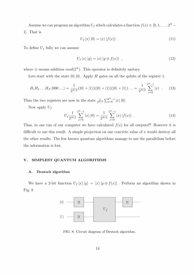
We have a 2-bit function Uf |x〉 |y〉 = |x〉 |y ⊕ f(x)〉. Perform an algorithm shown in
Fig. 8
H
H
H
Uf
|0〉
|1〉
FIG. 8: Circuit diagram of Deutsch algorithm.
14
1)
|ψ1〉 = H ⊗H |0〉 |1〉 =1
2(|0〉+ |1〉)(|0〉 − |1〉)
.
2)
|ψ2〉 = Uf |ψ1〉 =1
2[|0〉 (|f(0)〉 − |1⊕ f(0)〉) + |1〉 (|f(1)〉 − |1⊕ f(1)〉)]
|ψ2〉 =1
2
[(−1)f(0) |0〉+ (−1)f(1) |1〉
](|0〉 − |1〉)
3)
|ψ3〉 = H ⊗ 1 |ψ2〉 =1√2
± |0〉 ((|0〉 − |1〉)) if f(0) = f(1)
± |1〉 ((|0〉 − |1〉)) if f(0) 6= f(1)
Measuring the first qubit we can determine if f(0) = f(1) or f(0) 6= f(1). Note that Uf
was applied only once. Classically we would have to calculate f(x) twice in order to get the
same information.
A generalization to functions of arguments consisting of many qubits is called Deutsch-
Jozsa algorithm.
B. Quantum Fourier transform
A discrete Fourier transform a set of N complex numbers x0, x1, . . . , xN−1 into another
set y0, y1, . . . , yN−1 according
yk =1√N
N−1∑j=0
e2πijk/Nxj . (15)
This can be presented as unitary transformation UF . Indeed, assume we have a unitary
transformation on a register of n qubits defined as follows
UF |j〉 =1√2n
2n−1∑k=0
e2πijk/2n |k〉 . (16)
Then
UF2N−1∑j=0
xj |j〉 =1√2n
2n−1∑k=0
2N−1∑j=0
xje2πijk/2n |k〉 =
2n−1∑k=0
yk |k〉 . (17)
Quantum computer can implement UF efficiently. Introduce a phase shift gate
Rk =
1 0
0 e2πi/2k
. (18)
15

H
H R2 Rn−2 Rn−1
R2 Rn−1 Rn
H R2
H
jn−1
jn−2
jn−3
j1
j0 kn−1
kn−2
k1
k0
k2
FIG. 9: Quantum Fourier Transform. The input number is given by j =∑n−1m=0 jm2m.
The quantum Fourier transform is shown in Fig. 9. To understand this circuit we rewrite
(16) as
UF |jn−1, . . . , j0〉 =1√2n
∑k0,...,kn−1=0,1
exp
[2πi
n−1∑m=0
n−1∑l=0
jmkl2n−m−l
]|kn−1, . . . , k0〉 . (19)
We see that the number of gates needed for QFT is given by n+ (n−1) + (n−2) + . . .+ 1 =
n(n + 1)/2. The classical Fast Fourier Transform (FFT) needs O(n · 2n) gates. Thus the
quantum algorithm is much more efficient. As said above this efficiency in not so simple to
use.
C. Role of entanglement
Two qubits are called entangled if their state cannot be presented as a product state:
|ψprod〉 = (α1 |0〉 + β1 |1〉)(α2 |0〉 + β2 |1〉). For example the following state is entangled
(1/√
2)(|00〉+ |11〉).Consider a product state of all n qubits of a register.
|ψprod〉 =n−1∏m=0
(αm |0m〉+ βm |1m〉) . (20)
This state is parametrized by 2n real numbers (Bloch angles). Clearly a general state of
the register∑2n−1x=0 cx |x〉 is parametrized by many more numbers (2n− 2 complex numbers).
Thus the entanglement is behind the huge quantum capacity of the register.
16

VI. ONE-BIT MANIPULATIONS
A. Switching on the Hamiltonian for an interval of time
The simplest (in theory) way to perform a single-bit gate is to switch a Hamiltonian for
a finite interval of time ∆t. That is H(t) = g(t)V , where g(t < 0) = g(t > ∆t) = 0. The
gate operator is then given by
U = e−iθ2V , (21)
where hθ = 2∫dt g(t). For example if we chose V = σz we obtain
U = e−iθ2σz = cos
θ
2− i sin
θ
2σz (22)
Thus, choosing θ = π we obtain U = iσz. Since the total phase in not important we have
U = iZ ∼ Z. Analogously we can obtain gates X and Y .
Let us now choose θ = π/2 and V = σy. We then obtain
U =1√2
(1− i σy) =1√2
1 −1
1 1
. (23)
To obtain the Hadamard gate we have now to apply X = σx:
σx ·1√2
(1− i σy) =1√2
(σx + σz) = H . (24)
B. Rabi Oscillations
We consider a spin (qubit) in a constant magnetic field Bz and an oscillating field along
x axis:
H = −1
2Bz σz − ΩR cosωt σx . (25)
We use σx = σ+ + σ− and obtain
H = −1
2Bz σz −
1
2ΩR(eiωt + e−iωt)(σ+ + σ−) . (26)
We introduce the rotating frame. That is we introduce new wave functions like∣∣∣ψ⟩ =
R(t) |ψ〉. The Schrodinger equation for∣∣∣ψ⟩ reads
i∂t∣∣∣ψ⟩ = iR |ψ〉+RH |ψ〉 = iRR−1
∣∣∣ψ⟩+RHR−1∣∣∣ψ⟩ . (27)
17

Thus the rotating frame Hamiltonian reads
H = iRR† +RHR† . (28)
z
x y
FIG. 10: Rabi oscillations in the rotating frame.
FIG. 11: Rabi oscillations in the lab frame.
We chose a concrete R = exp(−iω σz
2t). Then
H = −1
2(Bz − ω) σz −
1
2ΩR(eiωt + e−iωt)(σ+e
−iωt + σ−eiωt) . (29)
H = −1
2(Bz − ω) σz −
1
2ΩRσx −
1
2ΩR(σ+e
−2iωt + σ−e2iωt) . (30)
The rotating wave approximation (RWA) gives
H = −1
2(Bz − ω) σz −
1
2ΩRσx . (31)
The simplest situation is at resonance ω = Bz. Then we have an effective magnetic field
ΩR in the x direction and the spin precesses around the x axis exactly as in the case of
Hamiltonian switching, but in the rotating frame (see Fig. 10 and Fig. 11). Note that the
18
Rabi frequency ΩR can be time-dependent. Then, the situation is exactly as in the previous
subsection and the angle of rotation θ is given by θ/2 =∫dtΩR(t). This is called the
”integral theorem”. A nice thing is that the rotation angle in only sensitive to the integral
of ΩR, thus higher fidelity of manipulations.
Consider now a phase shifted driving:
H = −1
2Bz σz − ΩR sinωt σx . (32)
This gives
H = −1
2Bz σz −
1
2iΩR(eiωt − e−iωt)(σ+ + σ−) . (33)
Further, in the rotating frame
H = −1
2(Bz − ω) σz −
1
2iΩR(eiωt − e−iωt)(σ+e
−iωt + σ−eiωt) . (34)
H = −1
2(Bz − ω) σz −
1
2ΩRσy −
1
2iΩR(σ+e
−2iωt − σ−e2iωt) . (35)
The rotating wave approximation (RWA) gives
H = −1
2(Bz − ω) σz −
1
2ΩRσy . (36)
Thus by choosing a different driving phase one can induce rotations around the y-axis in
the rotating frame. Usually both phases are used so that arbitrary manipulations can be
performed.
C. Simplest two-bit gates: iSWAP and√
iSWAP
We consider the following Hamiltonian:
H =J
4(σ(1)
x σ(2)x + σ(1)
y σ(2)y ) =
J
2(σ
(1)+ σ
(2)− + σ
(1)− σ
(2)+ ) , (37)
where σ± ≡ (σx ± iσy)/2. We have σ+ |1〉 = |0〉 and σ− |0〉 = |1〉. (This is somewhat
counterintuitive, because in spin physics we would call |0〉 = |↑〉 and |1〉 = |↓〉.)In the basis |00〉 , |01〉 , |10〉 , |11〉 this Hamiltonian reads
H =J
2
0 0 0 0
0 0 1 0
0 1 0 0
0 0 0 0
. (38)
19

It is clear that the operator e−iHt works as 1 in the subspace |00〉 , |11〉 and as e−iJ2σxt in the
subspace |01〉 , |10〉. Thus we obtain
e−iHt =
1 0 0 0
0 cos θ i sin θ 0
0 i sin θ cos θ 0
0 0 0 1
, (39)
where θ = −Jt/2. Choosing θ = π/2 we obtain iSWAP gate. If we disregard the multiplier
i this is a usual classical SWAP gate which swaps the two states of two qubits. However,
choosing θ = π/4 we obtain the purely quantum√
iSWAP gate. Clearly, this gate entangles
the two qubits.
VII. ADIABATIC MANIPULATIONS
A. Adiabatic ”theorem”
We consider the HamiltonianH = H0+V (t). Assume that the perturbation once switched
on remains forever (see Fig. 12).
t
V(t)
t 0
FIG. 12: Perturbation V (t) that does not disappear.
The evolution operator in the interaction representation reads
UI(t, t0) = T exp
− ih
t∫t0
dt′ VI(t′)
. (40)
Assume the initial state is the eigenstate |n〉 of H0. We obtain
|ΨI(t)〉 = UI(t, t0) |n〉 ≈1− i
h
t∫t0
dt′ VI(t′)
|n〉 , (41)
20
(Recall, |m〉 are the eigenstates of H0). The amplitude an→m in the expansion of the wave
function |ΨI(t)〉 is given by
an→m = − ih
t∫t0
dt′ Vmn(t′) eiωmnt′. (42)
We integrate by parts:
an→m = −Vmn(t′)
hωmneiωmnt
′∣∣∣tt0
+1
h
t∫t0
dt′(∂Vmn(t′)
∂t′
)eiωmnt
′
ωmn. (43)
At t0 there was no perturbation, V (t0) = 0, thus
an→m = −Vmn(t)
hωmneiωmnt +
1
h
t∫t0
dt′(∂Vmn(t′)
∂t′
)eiωmnt
′
ωmn. (44)
Let us try to understand the meaning of the first term of (44). Recall the time-
independent perturbation theory for Hamiltonian H = H0 + V . The corrected (up to
the first order) eigenstate |n〉 is given by
|n〉 ≈ |n〉 −∑m 6=n
VmnEm − En
|m〉 (45)
It is clear that the first term of (44) and the first order corrections in (45) have something
to do with each other (are the same). To compare we have to form in both cases the time-
dependent Schrodinger wave function. From (44) we obtain the interaction representation
wave function |ΨI〉 = |n〉+∑m6=n an→m(t) |m〉, which leads in the Schrodinger picture to
|Ψ(t)〉 = |n〉 e−iEnt/h −∑m6=n
VmnEm − En
|m〉 e−iEnt/h (46)
The same we get from (45) (upon neglecting corrections to the energy En).
Thus, the first term of (44) corresponds to the state ”adjusting” itself to the new Hamil-
tonian, i.e., remaining the eigenstate of the corrected Hamiltonian H = H0 +V . The ”real”
transitions an only be related to the second term of (44).
Idea of adiabatic approximation: if ∂Vmn(t)/∂t is small, than no real transition will
happen, and, the state will remain the eigenstate of a slowly changing Hamiltonian.
B. Transformation to the adiabatic (instantaneous) basis
New idea: follow the eigenstates of the changing Hamiltonian H(t). It is convenient to
introduce a vector of parameters ~χ upon which the Hamiltonian depends and which change
21

in time. H(t) = H(~χ(t)). We no longer consider a situation when only a small perturbation
is time-dependent. Diagonalize the Hamiltonian for each ~chi. Introduce instantaneous
eigenstates |n(~χ)〉, such that H(~χ) |n(~χ)〉 = En(~χ) |n(~χ)〉. Since H(~χ) changes continuously,
it is reasonable to assume that |n(~χ)〉 do so as well. Introduce a unitary transformation
R(t, t0) ≡∑n
|n(~χ(t0))〉 〈n(~χ(t))| =∑n
|n0〉 〈n(~χ(t))| . (47)
For brevity |n0〉 ≡ |n(~χ(t0))〉. Idea: if |Ψ(t)〉 ∝ |n(~χ(t))〉, i.e., follows adiabatically, the
new wave function: |Φ(t)〉 = R(t, t0) |Ψ(t)〉 ∝ |n0〉 does not change at all. Let’s find the
Hamiltonian governing time evolution of |Φ(t)〉:
ih∣∣∣Φ⟩ = ihR
∣∣∣Ψ⟩+ ihR |Ψ〉 = RH(t) |Ψ〉+ ihR |Ψ〉 =[RHR−1 + ihRR−1
]|Φ〉 (48)
Thus the new Hamiltonian is given by
H = RHR−1 + ihRR−1 (49)
The first term is diagonal. Indeed
R(t, t0)H(t)R(t0, t) =∑nm
|n0〉 〈n(~χ(t))|H(~χ(t)) |m(~χ(t))〉 〈m0|
=∑n
En(~χ(t)) |n0〉 〈n0| . (50)
Thus transitions can happen only due to the second term which is proportional to the time
derivative of R, i.e., it is small for slowly changing Hamiltonian.
C. Geometric Phase
The operator ihRR−1 may have diagonal and off-diagonal elements. The latter will be
responsible for transitions and will be discussed later. Here we discuss the role of the diagonal
elements, e.g.,
Vnn(t) = 〈n0| ihRR−1 |n0〉 = ih 〈n(~χ(t))|n(~χ(t))〉 = ih ~χ⟨~∇n(~χ)
∣∣∣n(~χ)〉 . (51)
This (real) quantity serves as an addition to energy En(~χ), i.e., δEn = Vnn. Thus, state
|n0〉 acquires an additional phase
δΦn = −∫dtδEn = −i
∫dt 〈n(~χ(t))|n(~χ(t))〉 . (52)
22

This phase is well defined only for closed path, i.e., when the Hamiltonian returns to
itself. Indeed the choice of the basis |n(~χ)〉 is arbitrary up to a phase. Instead of |n(~χ)〉 we
could have chosen e−iΛn(~χ) |n(~χ)〉. Instead of (51) we would then obtain
Vnn(t) = ih 〈n(~χ(t))|n(~χ(t))〉+ hΛn(~χ(t)) . (53)
Thus the extra phase is, in general, not gauge invariant. For closed path we must choose
the basis |n(~χ)〉 so that it returns to itself. That is |n(~χ)〉 depends only on the parameters
~χ and not on the path along which ~χ has been arrived. This means Λn(t0) = Λn(t0 + T ),
where T is the traverse time of the closed contour. In this case the integral of Λn vanishes
and we are left with
ΦBerry,n ≡ δΦn = −i∫dt 〈n(~χ(t))|n(~χ(t))〉 = −i
∫d~χ⟨~∇n
∣∣∣n〉 (54)
This is Berry’s phase. It is a geometric phase since it depends only on the path in the
parameter space and not on velocity along the path. Physical meaning (thus far) only for
superpositions of different eigenstates.
1. Example: Spin 1/2
FIG. 13: Time-dependent magnetic field.
We consider a spin-1/2 in a time-dependent magnetic field ~B(t): ~b = ~Ω × ~b, where
~b ≡ ~B/| ~B| and ~Ω is the angular velocity. The instantaneous position of ~B is determined by
the angles θ(t) and ϕ(t). The Hamiltonian reads
H(t) = −1
2~B(t) · ~σ (55)
23

We transform to the rotating frame with |Φ(t)〉 = R(t) |Ψ(t)〉 such that ~b is the z-axis in the
rotating frame. Here |Ψ〉 is the wave function in the laboratory frame while |Φ(t)〉 is the
wave function in the rotating frame. It is easy to find R−1 since it transforms a spin along
the z-axis (in the rotating frame) into a spin along ~B (in the lab frame), i.e., into the time
dependent eigenstate∣∣∣n( ~B(t))
⟩=∣∣∣↑ ( ~B(t))
⟩. Namely R−1 |↑z〉 =
∣∣∣↑ ( ~B(t))⟩. Thus
R−1(t) = e−iϕ(t)
2σz e−
iθ(θ)2
σy . (56)
This gives
RHR−1 = −1
2| ~B|σz (57)
and
iRR−1 = − θ2σy −
ϕ
2eiθ2σy σz e
−i θ2σy = − θ
2σy −
ϕ
2(cos θ σz − sin θ σx) . (58)
We can write
iRR−1 = −1
2~Ω · ~σ , (59)
where ~Ω = (−ϕ sin θ, θ, ϕ cos θ) is the angular velocity vector expressed in the rotating frame.
We obtain [iRR−1
]diag
= − ϕ2
cos θ σz (60)
For the Berry phase this would give
Φ↑/↓,Berry = ±1
2
∫ϕ cos θdt = ±1
2
∫Ω‖dt , (61)
where Ω‖ is the projection of the angular velocity on the direction of ~B (see Fig. 13). This
is however a wrong answer. What we forgot to check is wether the basis vectors return to
themselves after a full rotation θ(t0 +T ) = θ(t0), ϕ(t0 +T ) = ϕ(t0) + 2π. The operator that
transforms the eigenvector at t = t0 to the eigenvector at t = t0 + T is given by
R−1(t0 + T )R(t0) = e−iϕ+2π
2σz e−
iθ2σy e
iθ2σy ei
ϕ2σz = e−iπσz . (62)
Thus the states |↑ / ↓〉 get an extra phase ∓π. The correct, gauge invariant Berry’s phase
reads
Φ↑/↓,Berry = ±1
2
∫ϕ(cos θ − 1)dt = ±1
2
∫dϕ (cos θ − 1) . (63)
It is given by the solid angle (see Fig. 14).
24

FIG. 14: Solid angle.
D. Geometric interpretation
Once again we have a Hamiltonian, which depends on time via a vector of parameters
~χ(t), i.e., H(t) = H(~χ(t)). The Berry’s phase of the eigenvector |Ψn〉 is given by
Φn,Berry = i
t∫t0
〈Ψn|∂tΨn〉dt′ = i
t∫t0
〈Ψn|~∇~χΨn〉~χdt′ = i
t∫t0
〈Ψn|~∇~χΨn〉d~χ . (64)
We introduce a ”vector potential” in the parameter space
~An(~χ) ≡ 〈Ψn|i~∇~χ|Ψn〉 , (65)
which gives
Φn,Berry =∮C
~An(~χ)d~χ . (66)
Further
Φn,Berry =∫ (
~∇~χ × ~An)· d~S =
∫~Bn · d~S . (67)
Thus the Berry’s phase is given by the flux of an effective ”magnetic field” ~Bn ≡ ~∇~χ × ~An.
Clearly, one needs at least two-dimensional parameter space to be able to traverse a contour
with a flux through it (see Fig. 15).
E. Non-Abelian Berry Phase (Holonomy)
Imagine we have a degenerate subspace of N instantaneous eigenvectors. The rotating
frame Hamiltonian H = RHR−1 + ihRR−1, restricted to this subspace has the form
Hs,kl = const+ 〈k| ihRR−1 |l〉 . (68)
25

FIG. 15: Contour in the parameter space.
This matrix is not necessarily diagonal. Thus nontrivial evolution can happen in the sub-
space. We generalize the vector potential to a matrix
~Akl(~χ) ≡ 〈Ψk|i~∇~χ|Ψl〉 , (69)
The evolution operator in the subspace is a path ordered exponent
Us = Pei∮C~Akl(~χ)d~χ . (70)
Thus it is no longer ”only” a phase.
F. Non-adiabatic corrections: Transitions
1. Super-adiabatic bases
The Hamiltonian (49) in the adiabatic basis reads H = RHR1 + iRR−1. Lets call it H1 =
H. If the case is adiabatic , i.e., R(t) is slow, the new Hamiltonian H1(t) is also slow. We
can again find its instantaneous eigen-basis |n1(t)〉, such that H(t)1 |n1(t)〉 = E1(t) |n1(t)〉.We introduce the transformation R1 =
∑n |n(t)〉 〈n1(t)|. Transforming to the superadiabatic
basis |n1〉 we obtain the Hamiltonian
H2 = R1H1R−11 + iR1R
−11 . (71)
These iterations can be continued as suggested by Berry [1]. It seems that the rotation
R1 and further rotations R2, R3, . . . are closer and closer to 1. Indeed, since we have an
adiabatic case, R is small. Then, iRR−1 is also small and, since its the only term that is
non-diagonal in H1, the diaginalization R1 must be a very small rotation. Thus, |n1〉 is a
better approximation to the state of the system assuming it started in the eigenstate |n〉.
26

Berry showed that this logic works for a certain number of iterations and one can improve
the precision of adiabatic calculations. However at some point a problem arises: the series
H,H1, H2, . . . stops converging. It turns out to be an asymptotic series.
Let’s first understand what would happen if the superadiabatic iteration scheme would
always converge. Then the adiabatic theorem would be exact. Indeed, if we stated in a state
|n〉, during the evolution with the time-dependent H(t) we would be in the state |n∞〉 (since
the superadiabatic iteration converge). After the Hamiltonian stops changing in time, we
have H = H1 = H2 = . . . and the system is again in the state |n〉. Thus real transitions
never happen.
In reality transitions do happen. However, the slower is H(t) the better works the supera-
diabatic scheme and the transitions appear only after very many iterations. The transition
probability is thus very small. Below we investigate the transition probability.
2. Perturbation theory
We can treat the Hamiltonian (49) perturbatively. H(t) = H0(t) + V (t), where
H0(t) =∑n
En(~χ(t)) |n0〉 〈n0| , (72)
and
V (t) = ihRR−1 = ih∑n,m
|n0〉 〈n(~χ(t))|m(~χ(t))〉 〈m0| . (73)
H0 is diagonal, but time dependent. Interaction representation is simple to generalize:
|Φ(t)〉 ≡ e−(i/h)
t∫t0
dt′H0(t′)
|ΦI(t)〉 (74)
and
ihd
dt|ΦI〉 = VI(t) |ΦI〉 , (75)
where
VI(t) ≡ eit∫t0
dt′H0(t′)/h
V (t)e−i
t∫t0
dt′H0(t′)/h
(76)
(H0(t) commutes with itself at different times).
27

For the transition probability (of the first order) this gives
Pn→m ≈1
h2
∣∣∣∣∣∣∣∣∣iht∫
t0
dt′ 〈m(~χ(t′))|n(~χ(t′))〉 e−i
t′∫t0
dt′′[En(~χ(t′′))−Em(~χ(t′′))]/h
∣∣∣∣∣∣∣∣∣2
=
∣∣∣∣∣∣∣∣∣t∫
t0
dt′ 〈m(~χ(t′))|n(~χ(t′))〉 e−i
t′∫t0
dt′′[En(~χ(t′′))−Em(~χ(t′′))]/h
∣∣∣∣∣∣∣∣∣2
. (77)
3. Landau-Zener transition: perturbative solution
H(t) = −1
2(ε(t)σz + ∆σx) (78)
Parameter χ(t) = ε(t) = αt.
The eigenstates (dependent on χ)
|0(χ = ε)〉 = cos(η/2) |↑〉+ sin(η/2) |↓〉
|1(χ = ε)〉 = − sin(η/2) |↑〉+ cos(η/2) |↓〉 , (79)
where tan η ≡ ∆/ε. We find also the eigenenergies (dependent on χ = ε) E0/1 =
∓(1/2)√ε2 + ∆2.
ε
E0
E1
FIG. 16: Energy levels E0(ε) and E1(ε).
We obtain⟨1∣∣∣ 0〉 = −(1/2)η. From cot η = (αt/∆) we obtain η = − sin2 η(α/∆) =
− ∆α∆2+α2t2
. In the adiabatic basis the Schrodinger equation for the wave function |ψ〉 =
a(t) |0(ε)〉+ b(t) |1(ε)〉 reads
ihd
dt
a
b
= −1
2
√
∆2 + ε(t)2 −2ih⟨0∣∣∣ 1⟩
−2ih⟨1∣∣∣ 0⟩ −√∆2 + ε(t)2
a
b
. (80)
28

We obtain
ihd
dt
a
b
= −1
2
√
∆2 + α2t2 ih∆α∆2+α2t2
− ih∆α∆2+α2t2
−√
∆2 + α2t2
a
b
. (81)
There is a pair of special points in the complex t-plain t = ±t0 = ±i∆/α.
Assume that at t → −∞ the system was in the state |0(χ = ε = −∞)〉. What is the
probability that at t → ∞ a transition will happen to the state |1(χ = ε =∞)〉? From
Eq. (77) we obtain
P0→1 ≈
∣∣∣∣∣∣∣∣∞∫−∞
dt′⟨1∣∣∣ 0⟩ e(i/h)
t′∫0
dt′′√
∆2+α2t′′2
∣∣∣∣∣∣∣∣2
. (82)
(The lower limit of integration in the exponent was changed to 0, this just adds a constant
phase which does not change the probability).
For the transition probability this gives
P0→1 ≈
∣∣∣∣∣∣∣∣1
2
∞∫−∞
dt′∆α
∆2 + α2t′2e
(i/h)t′∫0
dt′′√
∆2+α2t′′2
∣∣∣∣∣∣∣∣2
. (83)
Introducing a new (dimensionless) time τ ≡ αt/∆ we obtain
P0→1 ≈
∣∣∣∣∣∣∣∣1
2
∞∫−∞
dτ ′1
1 + τ ′2eiγ
τ ′∫0
dτ ′′√
1+τ ′′2
∣∣∣∣∣∣∣∣2
, (84)
where γ ≡ ∆2/(hα). We see that the result depends only on γ.
Smart people (M. Berry) have calculated this integral and got
P0→1 ≈∣∣∣(π/3) e−
πγ4
∣∣∣2 = (π2/9) e−πγ2 . (85)
Problem: the result is non-analytic in α which characterizes the slowness of the change of
the Hamiltonian. Thus the logic of our perturbative expansion does not work. The result is
actually exponentially small for small enough α and not only small because it is proportional
to α. It cannot be excluded that higher order contributions will give also exponentially small
results.
29

4. Landau-Zener transition: quasi-classical solution in the adiabatic basis
Once again the Schrodinger equation in the adiabatic basis reads
ihd
dt
a
b
= −1
2
√
∆2 + α2t2 ih∆α∆2+α2t2
− ih∆α∆2+α2t2
−√
∆2 + α2t2
a
b
. (86)
We observe that the Hamiltonian has two special points in the complex plain: t = ±t0 = ± i∆α
(Fig. 17). For t → −∞ the system is in the state |0〉 = |↓〉. The asymptotic solution at
t→ −∞ reads
a ≈ exp
i
2h
t∫0
dτ√
∆2 + α2τ 2
. (87)
and b ≈ 0. Instead of solving the Schrodinger equation (86) on the real t-axis we ”go
Re t
Im t
t0
1
2
3
FIG. 17: Three contours.
around” in the complex plane. Let us investigate how the asymptotic Eq. (87) behaves if
we go along the contours 1, 2, 3 of Fig. 17. Since in (86)√
∆2 + α2τ 2 is assumed positive,
for τ → −∞ we obtain√
∆2 + α2τ 2 ≈ −ατ and a ≈ e−iαt2
4 . Along contour 3 (along the real
axis)√
∆2 + α2τ 2 remains positive. Thus, for τ → +∞ we have√
∆2 + α2τ 2 ≈ ατ . Thus,
along the real axis we obtain a ≈ eiαt2
4 for τ → +∞. This exponent corresponds to state
|0〉 = |↑〉. Thus contour 3 corresponds to the adiabatic evolution. On the other hand, along
contours 1 and 2 the solution a ≈ e−iαt2
4 remains the same at τ → −∞ and at τ → +∞. At
τ → +∞ this corresponds to the state |1〉 = |↑〉. These contours describe the Landau-Zener
transition. However we should have gotten the non-zero b. Let’s leave this task and go
further to the calculation in the diabatic basis.
30

5. Landau-Zener transition: quasi-classical solution in the diabatic basis
In the diabatic basis |↑ / ↓〉 the Schrodinger equation reads
ihd
dt
A
B
= −1
2
αt ∆
∆ −αt
A
B
. (88)
For t→ −∞ the system is in the state |↓〉, i.e. |A(−∞)| = 0 and |B(−∞)| = 1.
We obtain (h = 1) (id
dt+
1
2αt
)A = −∆
2B(
id
dt− 1
2αt
)B = −∆
2A . (89)
This gives (id
dt+
1
2αt
)(id
dt− 1
2αt
)B =
∆2
4B . (90)
Further (− d2
dt2− α2t2
4− iα
2
)B =
∆2
4B . (91)
We attempt a semiclassical solution A = eiS and obtain
S2 − iS =α2t2 + ∆2
4+iα
2. (92)
We again ”go around” the point t = 0 along a contour such that everywhere α2|t|2 ∆2.
Then we can perform an expansion in ∆/(αt). We write S = S0 +S1 and obtain S0 = −αt2
4.
For S1 we obtain
2S0S1 + S21 − iS1 =
∆2
4. (93)
Leaving only the first term in the RHS we obtain
S1 = −∆2
4αt= − γ
4t. (94)
This gives
S1 = −γ4
ln t+ const. (95)
(the constant should be chosen so that S1 is real for t → −∞). Upon the traversal of the
contour (in the upper half-plane) the function S1 acquires an imaginary part
Im[S1] =πγ
4. (96)
31

Re t
Im t1
2
3
4
FIG. 18: Stokes lines. In complex analysis a Stokes line, named after Sir George Gabriel Stokes,
is a line in the complex plane which ’turns on’ different kinds of behaviour when one ’passes over’
this line. Somewhat confusingly, this definition is sometimes used for anti-Stokes lines.
The question is whether we choose a contour in the lower or in the upper half-plane. The
asymptotic solution for t→ −∞ reads ei S0 = e−iαt2
2 . In Fig. 18 the so called Stokes lines are
shown on which e−iαt2
2 is real. On Stokes lines 1 and 3 the function e−iαt2
2 is exponentially
small (decreases with increasing |t|). On Stokes lines 2 and 4 the function e−iαt2
2 is expo-
nentially large(increases with increasing |t|). We start from the negative real axis on which
B ≈ e−iαt2
2 . If we would continue in the lower half-plane this solution would first become
exponentially large at line 4. There another solution eiαt2
2 would be exponentially small.
This another solution would become large on line 3 where the original solution is small and
we should ”drop”. On the other hand, if we continue in the upper half-plain the solution
e−iαt2
2 first becomes small at line 1. However we do not have there the big solution eiαt2
2
since it was not there on the real negative axis. This we continue with the solution e−iαt2
2
all the way to the positive real axis.
The transition probability, thus, reads
P0→1 =|B(+∞)|2|B(−∞)|2 = e−2Im[S1] = e−
πγ2 . (97)
6. Landau-Zener transition: exact solution
The exact result is known (Landau 1932, Zener 1932, Stuckelberg 1932, Majorana 1932).
It reads: P0→1 = e−πγ2 for arbitrary γ.
32

VIII. OPEN QUANTUM SYSTEMS
In the undergraduate course it is mostly assumed that the quantum system of interest
is completely isolated from its surroundings. The state of the system is described by a
vector |ψ(t)〉, and its time evolution is given by the unitary operator e−iHt where H is the
Hamiltonian of the system. If the system is controlled coherently, e.g. by a laser field, or
by an external magnetic field, it is strictly speaking not a closed system any more, because
of its interaction with the external field. However, in many cases this interaction can be
accounted for by a modification of the Hamiltonian (which might now be time-dependent),
and we can still treat the system like a closed system. In such cases, we say the system
interacts with a “classical” field.
However, there are many situations in which this is not the case. As a simple example
consider qubit A as the system of interest, which interacts with another qubit B which is
initially in the state |0〉. We use the interaction Hamiltonian Eq. (38) and choose t = −π/Jto obtain an iSWAP gate, which essentially swaps the states of the two states. The evolution
of qubit A is:
|ψ(0)〉 = |0〉 → |ψ(t)〉 = |0〉
|ψ(0)〉 = |1〉 → |ψ(t)〉 = |0〉 (98)
No unitary evolution operator acting on the Hilbert space HA of qubit A results in such a
transformation!!! Of course, this transformation can be described by a unitary operator in
the larger Hilbert space HA ⊗HB.
In real experiments, the system of interest often interacts with an environment E (e.g. a
bath in its thermal equilibrium) with infinitely degrees of freedom. It is a hopeless task to
find the total evolution operator in HA⊗HE, and often the state and / or the Hamiltonian
of E is not known. We have to find other methods, and that is the aim of the theory of open
quantum systems. We follow in part the book of Breuer and Petruccione (see literature list).
An environment generally has the following effects on a quantum systems
• Decoherence: Superpositions of macroscopically distinct states are strongly sup-
pressed.
• Dephasing: Off-diagonals of the density matrix in the basis of the energy eigenstates
33

get reduced. This can have two causes: Phase averaging if the energy is not known
exactly (sometimes reversible by spin echo), and decoherence (non-reversible)
• Dissipation: Exchange of energy between system and environment. This changes
the populations of the density matrix and eventually leads to the equilibrium state
ρS(t→∞) = 1Ze−H/kBT at the temperature of the environment.
A. Density operator
We can formulate quantum mechanics using either state vectors |ψ〉, or state operators
ρ (usually referred to as density operator). The table I shows a brief comparison:
State vector Density operator
State |ψ〉 ρ = |ψ〉〈ψ|
Time evolution ddt |ψ〉 = −iH |ψ〉 d
dtρ = −i[H, ρ]
Expectation value of O 〈ψ|O |ψ〉 Tr(ρO)
Probability of measuring m |〈m |ψ〉 |2 〈m| ρ |m〉
TABLE I: State vectors and density operators for pure states
The density operator formalism has two big advantages:
• Statistical mixtures: We do not know the state with certainty, but we know that
with probability pj we are in the state |ψj〉. In the state vector formalism, we have to
evolve all states |ψj〉, calculate each expectation value 〈O〉j = 〈ψj|O |ψj〉 and take the
average 〈O〉 =∑j〈O〉j (same for probabilities). In the density operator formalism we
just use ρ =∑j pj |ψj〉〈ψj|, and continue as with a pure state.
• Subsystems: If the state vector of a composite system AB is |ψAB〉, we can generally
not assign a state vector to the subsystems A and B (→ entanglement). However, we
can always describe the subsystems by a density operator which is obtained by the
partial trace of the density operator of the composite system, e.g. ρA = TrBρAB.
The first property is very useful in statistical mechanics, while the second is very valuable
for open quantum systems, where the system S of interest is part of a much larger composite
system SE.
34

A density operator has the following properties:
• Tr(ρ)=1 (→ sum of all probabilities)
• Tr(ρ2) ≤ 1, “=” if and only if the system is in a pure state.
• ρ† = ρ
• ρ ≥ 0: Eigenvalues between zero and one (→ probabilities)
Different physical situations can lead to the same density matrix. Consider the Bell states
|φ±〉 = (|00〉 ± |11〉)/√
2. Both result in reduced density operators ρA = ρB = 1l/2, as do
the other two Bell states, or an equal mixture of all pure states (this describes the situation
in which we have no information about the state). This imposes the question whether the
density operator formalism is sufficient to describe all physical situations. The answer is a
definite yes if one is interested in the prediction of probabilities of measurement outcomes
only, as is usually the case in any physical theory. More precisely, it can be shown that
no measurement on system A can distinguish between two physical situations which are
described by the same density operator ρA.
Just like an operator defines a linear transformation in Hilbert space, a linear transfor-
mation in operator space (called Liouville space) is called a super operator. We denote these
with calligraphic fonts. For a super operatorM to define a valid transformation of a density
operator, it has to preserve the above properties. Therefore M has to be trace preserving
and positive. The latter means thatMρ ≥ 0 if ρ ≥ 0. Actually, to demand positivity is not
sufficient, alsoM⊗ 1l has to be positive for the identity operator in any dimension. This is
called completely positive, and reflects the fact that transforming the system with M and
doing nothing to another system on the moon still results in a positive density operator.
Every trace preserving, completely positive transformation (called a quantum map) can
be written with Kraus operators Kj
Mρ =∑j
KjρK†j , with
∑j
K†j Kj = 1l. (99)
This representation theorem for quantum operations is due to Kraus. A unitary transfor-
mation is a special case of a quantum map. An example for a non-unitary transformation
is Eq. (98), which is achieved with K0 = |0〉〈0| and K1 = |0〉〈1|.
35
unitär
Schrödinger Gl.
nicht unitär
master Gleichung
TrE Tr
E
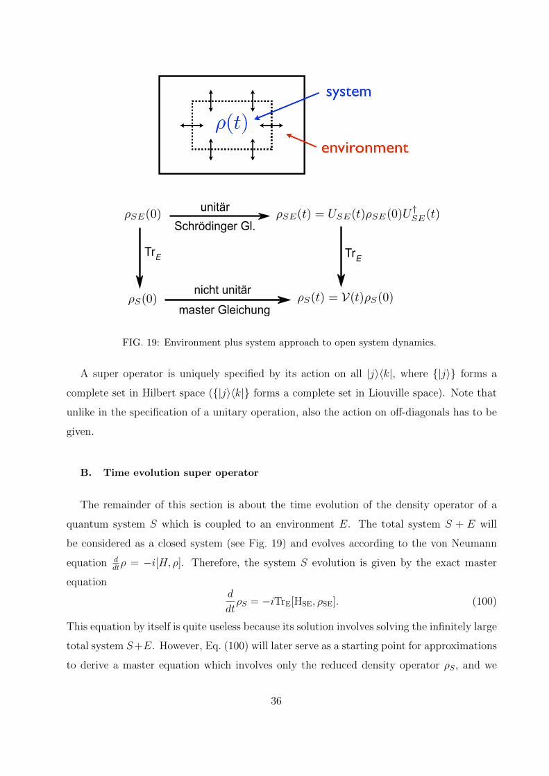
FIG. 19: Environment plus system approach to open system dynamics.
A super operator is uniquely specified by its action on all |j〉〈k|, where |j〉 forms a
complete set in Hilbert space (|j〉〈k| forms a complete set in Liouville space). Note that
unlike in the specification of a unitary operation, also the action on off-diagonals has to be
given.
B. Time evolution super operator
The remainder of this section is about the time evolution of the density operator of a
quantum system S which is coupled to an environment E. The total system S + E will
be considered as a closed system (see Fig. 19) and evolves according to the von Neumann
equation ddtρ = −i[H, ρ]. Therefore, the system S evolution is given by the exact master
equationd
dtρS = −iTrE[HSE, ρSE]. (100)
This equation by itself is quite useless because its solution involves solving the infinitely large
total system S+E. However, Eq. (100) will later serve as a starting point for approximations
to derive a master equation which involves only the reduced density operator ρS, and we
36

will go this path in the following subsection.
The formally define the time evolution super operator
ρS(t) = VS(t)ρS(0), (101)
which, of course, has to be trace preserving and completely positive[11], but might not be
invertible. Along the lines of the diagram in Fig. 19 we can easily see that VS(t) has a Kraus
operator representation if we use ρSE(0) = ρS(0)⊗ ρE(0) and ρE =∑α λα |ϕα〉〈ϕα|
VS(t)ρS(0) = TrE[USE(t)ρS(0)⊗ ρE(0)U †SE(t)
]=∑αβ
〈ϕβ|USE(t) |ϕα〉√λαρS(0)
√λα 〈ϕα|USE(t) |ϕβ〉
=∑αβ
KαβρS(0)K†αβ. (102)
Note that Wαβ are operators in the HS. This equation shows that the dynamics which are
obtained by the coupling to an environment are trace preserving and completely positive.
But for further calculations, it is not very useful because we do not know USE(t).
Instead we pursue another path. If we assume that
VS(t1 + t2) = VS(t1)VS(t2), (103)
then the set VS(t) forms a semi group and therefore has a generator
VS(t) = exp(Lt). (104)
This immediately yield a first-order differential equation for the reduced density matrix
d
dtρS(t) = LρS(t) (105)
where L is called the Liouville super operator or Liouvillian. For a closed system, the Liou-
villian is given by the commutator with the Hamiltonian, i.e. LρS = −i[HS, ρS]. A master
equation of the form Eq. (105) is called a Markovian master equation, i.e. the evolution at
time t only depends on the state of the system at this time.
A general master equation is not Markovian and can not be brought into the form
Eq. (105). The reason is that the system S continuously changes the state of the envi-
ronment. As a result, the system at time t interacts with an environmental state which
37

depends on the systems state at all times 0 < t′ < t and the assumption Eq. (102) is not
justified. The most general master equation can be written as
d
dtρS(t) =
∫ t
0dt′K(t− t′)ρS(t′), (106)
where K(t−t′) is called the memory kernel. If the memory time is short, we can approximate
K(t− t′) ≈ δ(t− t′)L to get a Markovian master equation.
Lindblad [2] as well as Gorini, Kossakowski, and Sudarshan [3] showed that the most
general form of a Markovian master equation which preserves the trace and positivity is
d
dtρS = −i[H, ρS] +
N2−1∑k=1
γk
(LkρSL
†k −
1
2L†kLkρS −
1
2L†kLk
). (107)
This master equation is said to be in Lindblad form. The Hamiltonian H is generally not
HS but might also include coherent corrections due to the environment like the Lamb shift.
The incoherent evolution is represented by at most N2 − 1 Lindblad operators Lk where
N is the dimension of the Hilbert space HS. The γk are the rates for the quantum jumps
ρS → LkρSL†k and can be absorbed into the Lindblad operators.
C. Microscopic derivations of master equations
In this subsection we derive a Markovian master equation for ρS from the underlying
physics of S + E. In doing so, we will perform a number of approximation which we will
discuss at the end. The Hamiltonian of S + E is
HSE = HS +HE +HI , (108)
where HI =∑j Aj ⊗Bj is the interaction Hamiltonian and A acts on HS and B on HE. As
before, we will assume that initially the system and the environment are not correlated, i.e.
ρSE(0) = ρS(0)⊗ρE, and also that the environment is at equilibrium at temperature T such
that eiHEtρEe−iHEt = ρE. We proceed by going into the interaction picture by transforming
the von Neumann equation with ei(HS+HE)t to find
d
dtρSE(t) = −i[HI(t), ρSE(t)] (109)
ρSE(t) = ρSE(0)− i∫ t
0ds [HI(s), ρSE(s)], (110)
38

where HI(t) = A(t)⊗B(t) = eiHStAe−iHSt ⊗ eiHEtBe−iHEt (for simplicity we do not use the
most general interaction Hamiltonian). We now substitute the integral version Eq. (110)
into Eq. (109), then take the trace over E :
d
dtρS(t) = −iTrE[HI(t), ρSE(0)]− TrE
∫ t
0ds [HI(t), [HI(s), ρSE(s)]]
(111)
Our first assumption is that
TrE[HI(t), ρSE(0)] = 0 (112)
which will by mathematically motivated later. Physically it means that the dynamics at
time t should not depend on the state ρS(0) at time t = 0.
d
dtρS(t) = −
∫ t
0dsTrE[HI(t), [HI(s), ρSE(s)]] (113)
This is still not a closed equation for ρS because ρSE still appears on the right hand side.
We substitute the Born approximation
ρSE(s) = ρS(s)⊗ ρE (114)
which states that the environment does not get disturbed by the system, and get a closed
equation for ρS:
d
dtρS(t) = −
∫ t
0dsTrE[HI(t), [HI(t− s), ρS(t− s)⊗ ρE]] (115)
We also substituted s by t − s. This equation is not Markovian because ρS is not only
needed at time t, but at all times between zero and t. We therefore perform the Markov
approximation
ρS(t− s) = ρS(t) (116)
which is valid if the integrand vanishes for large s.
d
dtρS(t) = −
∫ t
0dsTrE[HI(t), [HI(t− s), ρS(t)⊗ ρE]]. (117)
This so called Redfield equation still does not describe a semi group because the generator
explicitly depends on time t through the integration range. But because the integrand is
assumed to vanish for larch s, we can extend the integration to infinity to arrive at the
Markovian master equation
d
dtρS(t) = −
∫ ∞0
dsTrE[HI(t), [HI(t− s), ρS(t)⊗ ρE]]. (118)
39

By substituting HI(t) = A(t)⊗B(t) and some simple algebra we finally find
d
dtρS(t) =
∫ ∞0
dsΓ(s)[A(t− s)ρS(t)A(t)† − A†(t)A(t− s)ρS(t)
]+ h.c., (119)
where h.c. stands for hermitian conjugate and where we defined the bath correlation function
Γ(s) = TrE[B(s)BρE]. (120)
It is interesting to see that no details of the environment are needed, only the bath correlation
function is important.
Let us review the approximations we have done so far:
• Eq. (112): This requires TrE[B(t)ρE] = 0. Imagine that this trace is not zero, then it
is still a constant c because ρE is stationary. We can write HI = A⊗(B−c1l)+cA. If we
absorb bA into the system Hamiltonian then the new HI fulfills Eq. (112). Therefore
this is not an approximation but can always be fulfilled exactly.
• Born appr.: This means that the coupling HI is weak and the environment is large
such that the system can not change the state of the environment. Typically the
system can excite the environment, but as long as the excitation decays rapidly the
system will still see the environment in a thermal equilibrium (time average of ρE).
• Markov appr.: The integrand vanishes if the bath correlation function vanishes.
When the bath correlation function vanishes on a time τB, then this approximation is
satisfied if HI does not change the state appreciably during τB.
• t→∞: The extension of the integrand requires a fast decay of Γ(s).
Everything therefore depends on a fast decay of the bath correlation function. For this
to be valid we have to know that E has many degrees α of freedom and the system couples
to many of them B =∑α bα, and therefore 〈B(s)B〉 =
∑α〈bα(s)bα〉. Each 〈bα(s)bα〉 has
its specific time behavior, often oscillating with some transition frequency of the degree α.
The average of all these oscillations typically is zero unless at time s = 0 because for each
degree of freedom 〈b2α〉 > 0. To ensure that there is no beating one need an infinite number
of degrees of freedom. See also Fig. 20.
The master equation Eq. (119) can not be written in Lindblad form. Therefore it can
result in negative probabilities, which we will discuss later. We will now cast the ME into
40

5 10 15 20 25 30
2
1
1
2
3
4
t
FIG. 20: The sum of the oscillations has a pronounced initial peak, and decays over a time τB. The
more frequencies, the better the decay. If the number of frequencies is finite, the bath correlation
will reoccur at some time. Therefore, the bath needs to have an infinite number of degrees of
freedom for our approximations to be valid.
Lindblad form by performing the so called secular approximation. For simplicity we consider
only a two-level system, but the generalization is straight forward.
We first decompose A into eigen operators of the Hamiltonian
A =∑
jk=e,g
〈j|A |k〉 |j〉〈k| = A0 + A1 + A−1
A0 = 〈g|A |g〉 |g〉〈g|+ 〈e|A |e〉 |e〉〈e|
A1 = 〈e|A |g〉 |e〉〈g|
A−1 = 〈g|A |e〉 |g〉〈e| . (121)
This has that advantage the Aj can be transformed into the interaction picture by multipli-
cation with a phase factor
Aj(t) = e−iωjtAj (122)
with
ω−1 = Ee − Egω0 = 0
ω1 = Eg − Ee. (123)
41

From Eq. (119) we obtain
d
dtρS(t) =
1∑jk=−1
∫ ∞0
dsΓ(s)e−iωj(t−s)eiωkt[AjρS(t)A†k − A†kAjρS(t)
]+ h.c.,
=1∑
jk=−1
Γ(ωj)ei(ωk−ωj)t
[AjρS(t)A†k − A†kAjρS(t)
]+ h.c., (124)
where we have defined the Laplace transform of the bath correlation functions
Γ(ω) =∫ ∞
0dsΓ(s)eiωs (125)
If the interaction to the environment is small compared to (ωk − ωj), the we can use the
RWA, which in this context is called the secular approximation, and only keep terms with
ωk = ωj (see Exercise 1):
d
dtρS(t) =
1∑j=−1
Γ(ωj)[AjρS(t)A†j − A†jAjρS(t)
]+ h.c.. (126)
If Γ(ωj) were positive, then this equation would be in Lindblad form. We now separate the
imaginary part from the real part
Γ(ω) =1
2γ(ω) + i ImΓ(ω) (127)
and by substituting into Eq. (126) we see that the AjρS(t)A†j cancels in the imaginary
contribution. We find
d
dtρS(t) = −i[HLS, ρS] +
1∑j=−1
γ(ωj)[AjρS(t)A†j −
1
2A†jAjρS(t)− 1
2ρS(t)A†jAj
], (128)
where we defined the Lamb shift Hamiltonian
HLS =1∑
l=−1
ImΓ(ωj)A†jAj. (129)
We finally transform back into the Schrodinger picture
d
dtρS(t) = −i[HS +HLS, ρS] +
1∑j=−1
γ(ωj)[AjρS(t)A†j −
1
2A†jAjρS(t)− 1
2ρS(t)A†jAj
]. (130)
This is our final master equation, which is in Lindblad form and therefore guarantees a
positive density operator. The Lamb shift is an energy shift of the system induced by the
environment, but it does not change the eigenstates of the system because [HLS, HS] = 0.
42

z
y
x
z
y
x
z
y
x
Relaxation Excitation Dephasing(a) (b) (c)
z
y
x
X
(d) Flow towards the steady state
FIG. 21: The effect of the Lindblad terms on the qubit in the interaction picture. In the Schrodinger
picture, there is an additional rotation around the z-axis.
The incoherent part of the evolution is due to the Lindblad term, which is often called
dissipator.
The environment usually has all different frequencies. However, only the frequencies
which are transition frequencies of the system can induce transitions, e.g. γ(Ee−Eg) induces
relaxations [see Fig. 21 (a)] and γ(Eg − Ee) induces excitations [see Fig. 21 (b)]. The
slow frequencies of the environment, i.e. γ(0), can not change the population of the energy
eigenstates, but reduces the off-diagonals (dephasing) [see Fig. 21 (c)].
The ME has a steady state [see Fig. 21 (d)] with
ρeg(t→∞) = 0 (131)
ρz(t→∞) = −γ(Ee − Eg)− γ(Eg − Ee)γ(Ee − Eg) + γ(Eg − Ee)
(132)
where ρz = ρee − ρgg.
43

The time evolution is given by (see exercise 2)
ρeg(t) = ρeg(0)ei(Eg−Ee)te−t/T2 (133)
ρz(t) = ρz(∞) + [ρz(0)− ρz(∞)]e−t/T1 (134)
The relaxation time T1 depends on γ(ω 6= 0) and on the off-diagonal matrix elements of A.
For the dephasing time one can write
T−12 = T−1
1 /2 + (T ∗2 )−1, (135)
where (T ∗2 )−1 is called the pure dephasing rate and depends on γ(ω = 0) and on the diagonal
matrix elements of A. Eq. (135) shows that there can not be energy relaxation without
dephasing, while it is possible to have pure dephasing without energy relaxation.
Quantum opticians almost only use such a ME of Lindblad form because of its simplicity
and because all the approximations are very well satisfied in typical quantum optics applica-
tions. The predictions based on this ME can very accurately describe experiments. In solid
state physics, people often don’t like this equation because the weak coupling and the short
bath correlation time τB are often not satisfied. However, for quantum computing devices
we can only use systems which are very weakly coupled to any environment. Therefore, the
description of a qubit on the basis of a Lindblad equation is well justified.
1. Relation to the correlation function
In the derivation of the Lindblad master equation we have defined a correlation function
Γ(t) = C(t) = TrE[B(t)BρE] , (136)
where ρE denotes the density matrix of the environment (bath) in thermal equilibrium. The
additional notation C(t) is introduced for convenient and consistency with the literature,
where a correlator is called C. Further we have defined the Laplace transform
Γ(ω) =∫ ∞
0dtΓ(t)eiωt . (137)
The Laplace transform Γ(ω) gives both the dissipative rates γ(ω) = 2ReΓ(ω) and the Lamb
shift (renormalization) via ImΓ(ω). We now find the relation between these quantities and
the Fourier transform of the correlation function
C(ν) =
∞∫−∞
C(t)eiνt dt . (138)
44

Note, that C(ν) is real, since C(−t) = C∗(t). The last equation holds because B is hermitian.
We obtain
Γ(ω) =∫ ∞
0dtC(t)eiωt−δt =
∫ ∞0
dt eiωt−δt∫ dν
2πC(ν)e−iνt
=∫ dν
2πC(ν)
1
iν − iω + δ= i
∫ dν
2πC(ν)
1
ω − ν + iδ. (139)
Thus we obtain
Re Γ(ω) =1
2C(ω) , γ(ω) = C(ω) . (140)
Im Γ(ω) = P.V.∫ dν
2πC(ν)
1
ω − ν (141)
2. Lamb shift for a two-level system
It is interesting to calculate the Lamb shift for a 2-level system. We have derived
HLS =1∑
l=−1
ImΓ(ωj)A†jAj. (142)
From (121) we see that
A0 = a1 + bσz , A1 = c σ− , A−1 = c∗σ+ . (143)
(recall that |g〉 = |0〉 = |↑〉). We should also take a = 0, since this part does not give a
coupling between the qubit and the bath. We obtain
HLS = b2ImΓ(0) + |c|2 ImΓ(ω1)(
1
2+
1
2σz
)+ |c|2 ImΓ(−ω1)
(1
2− 1
2σz
)= const− σz
2|c|2
[ImΓ(−ω1)− ImΓ(ω1)
], (144)
where ω1 = Eg − Ee = −∆E. This
HLS = −1
2δ∆E σz (145)
with the renormalization of the energy difference given by
δ∆E = |c|2P.V.∫ dν
2π
[C(ν)
(∆E − ν)− C(ν)
(−∆E − ν)
]= |c|2P.V.
∫ dν
2π
[C(ν) + C(−ν)
∆E − ν
](146)
Introducing the symmetrized correlator S(ν) ≡ 12(C(ν) + C(−ν)) we, finally, obtain
δ∆E = |c|2P.V.∫ dν
2π
2S(ν)
(∆E − ν)= −|c|2P.V.
∫ dν
2π
2∆ES(ν)
(ν2 − (∆E)2). (147)
45

D. Golden Rule calculation of the energy relaxation time T1 in a two-level system
We now analyze the dissipative processes in two-level systems (qubits) is a more detailed
fashion. The goal is to develop a deeper understanding. Let us first consider a purely
transverse coupling between a qubit and a bath
H = −1
2∆E σz −
1
2X σx +Hbath , (148)
where X is a bath operator. To compare with the previous section we have A = −(1/2)σx
and B = X. We denote the ground and excited states of the free qubit by |0〉 and |1〉,respectively. In the weak-noise limit we consider X as a perturbation and apply Fermi’s
golden rule to obtain the relaxation rate, Γ↓ = Γ|1〉→|0〉, and excitation rate, Γ↑ = Γ|0〉→|1〉.
For the relaxation the initial state is actually given by |1〉 |i〉, where |i〉 is some state of the
environment. This state is not known, but we assume, that the environment is in thermal
equilibrium. Thus the probability to have state |i〉 is given by ρi = Z−1e−βEi (Hbath |i〉 =
Ei |i〉). The final state is given by |0〉 |f〉, where |f〉 is the state of the environment after the
transition. To obtain the relaxation rate of the qubit we have to sum over all possible |i〉states (with probabilities ρi) and over all |f〉. Thus, for Γ↓ we obtain
Γ↓ =2π
h
∑i,f
ρi | 〈i| 〈1|1
2Xσx |0〉 |f〉 |2 δ(Ei + ∆E − Ef )
=2π
h
1
4
∑i,f
ρi | 〈i|X |f〉 |2 δ(Ei + ∆E − Ef )
=2π
h
1
4
∑i,f
ρi 〈i|X |f〉 〈f |X |i〉1
2πh
∫dt ei
th
(Ei+∆E−Ef )
=1
4h2
∫dt∑i
ρi 〈i|X(t)X |i〉 ei th ∆E
=1
4h2 CX(ω = ∆E/h) =1
4h2 〈X2ω=∆E/h〉 . (149)
Similarly, we obtain
Γ↑ =1
4h2 CX(ω = −∆E/h) =1
4h2 〈X2ω=−∆E/h〉 . (150)
How is this all related to the relaxation time of the diagonal elements of the density
matrix (T1)?. To understand this we write down the master equation for the probabilities
p0 = ρ00 and p1 = ρ11:
p0 = −Γ↑p0 + Γ↓p1
p1 = −Γ↓p1 + Γ↑p0 . (151)
46

We observe that the total probability p0 + p1 is conserved and should be equal 1. Then for
p0 we obtain
p0 = −(Γ↑ + Γ↓)p0 + Γ↑ , (152)
which gives
p0(t) =Γ↓
Γ↑ + Γ↓+
(p0(0)− Γ↓
Γ↑ + Γ↓
)e−(Γ↑+Γ↓)t , (153)
and p1(t) = 1− p0(t).
For the relaxation time we thus find
1
T1
= Γ↓ + Γ↑ =1
2h2 SX(ω = ∆E/h) , (154)
and for the equilibrium magnetization
〈σz〉t=∞ = p0(t =∞)− p1(t =∞) =Γ↓ − Γ↑Γ↓ + Γ↑
=AX(ω = ∆E/h)
SX(ω = ∆E/h), (155)
where we have introduced the antisymmetrized correlator AX(ω) ≡ 12(CX(ω)− CX(−ω)).
E. Fluctuation Dissipation Theorem (FDT)
Are C(ω) and C(−ω) related? In other words, what is the relation between the sym-
metrized correlator S(ω) and the antisymmetrized one A(ω)? We use the spectral decom-
position in the eigenbasis of the Hamiltonian of the environment Hbath |n〉 = En |n〉:
C(t) = Tr(ρEB(t)B) =1
Z
∑n
e−βEn 〈n|B(t)B |n〉
=1
Z
∑n,m
e−βEn 〈n|B(t) |m〉 〈m|B |n〉 =1
Z
∑n,m
e−βEnei(En−Em)t| 〈m|B |n〉 |2 . (156)
Thus
C(ω) =∫dtC(t)eiωt =
1
Z
∑n,m
e−βEn| 〈m|B |n〉 |2 2πδ(ω − (Em − En)) . (157)
For C(−ω) we obtain
C(−ω) =1
Z
∑n,m
e−βEn| 〈m|B |n〉 |2 2πδ(−ω − (Em − En))
=1
Z
∑n,m
e−βEn| 〈m|B |n〉 |2 2πδ(ω − (En − Em))
=1
Z
∑n,m
e−βEm| 〈m|B |n〉 |2 2πδ(ω − (Em − En))
=1
Z
∑n,m
e−β(En+ω)| 〈m|B |n〉 |2 2πδ(ω − (Em − En))
= e−βω C(ω) . (158)
47

The relation C(−ω) = e−βωC(ω) is called the Fluctuation-Dissipation-Theorem (this time
a real theorem). A simple algebra then gives S(ω) = coth(βω2
)A(ω). Thus we obtain the
detailed balance relationΓ↑Γ↓
= e−β∆E . (159)
We also observe that the probabilities p0(t =∞) = 1e−β∆E+1
and p1(t =∞) = 1− p0(t =∞)
are the equilibrium ones. Finally,
〈σz〉t=∞ =AX(ω = ∆E/h)
SX(ω = ∆E/h)= tanh
∆E
2kBT. , (160)
F. Longitudinal coupling, T ∗2
H = −1
2∆E σz −
1
2X σz +Hbath , (161)
1. Classical derivation
Treating X as a classical variable one obtains
〈σ+(t)〉 ∝⟨e− ih
t∫0
dt′X(t′)⟩
= e− 1
2h2
t∫0
dt′t∫
0
dt′′〈X(t′)X(t′′)〉
= exp
(− 1
2h2
∫ dω
2πSX(ω)
sin2(ωt/2)
(ω/2)2
). (162)
If we make the usual Golden Rule substitution sin2(ωt/2)/(ω/2)2 → 2πδ(ω) t in Eq. (162)
we obtain
lnP (t) = − 1
2h2SX(ω = 0) t . (163)
Thus we obtain1
T ∗2=
1
2h2SX(ω = 0) . (164)
When both longitudinal and transverse coupling are present one obtains for the dephasing
time1
T2
=1
2T1
+1
T ∗2. (165)
How about 1/f noise? Is 1/T ∗2 infinite?
48

2. Quantum derivation
We calculate the time evolution of the off-diagonal element of the qubit’s density matrix:
〈σ+(t)〉 = e−i∆Eth Tr
[σ+ S(t, 0)ρ0 S
†(t, 0)], (166)
where
S(t, 0) ≡ Te
ih
t∫0
X(t′)2
σz dt′
. (167)
Obviously, the evolution operators S and S† do not flip the spin, while the operator σ+ in
Eq. (166) imposes a selection rule such that the spin is in the state |↓〉 on the forward Keldysh
contour (i.e., in S(t, 0)) and in the state |↑〉 on the backward contour (i.e., in S†(t, 0)). Thus,
we obtain 〈σ+(t)〉 = P (t) exp(−i∆Et/h)〈σ+(0)〉, where
P (t) ≡ 〈T exp
− ih
t∫0
X(t′)
2dt′
T exp
− ih
t∫0
X(t′)
2dt′
〉 . (168)
The last expression can be represented as a single integral on the Keldysh contour C:
P (t) ≡ 〈TC exp
(− ih
∫C
X(t′)
2dt′)〉 . (169)
Using the fact that the fluctuations of X are Gaussian, we arrive at
lnP (t) = − 1
8h2
∫C
∫Cdt1dt2〈TCX(t1)X(t2)〉 . (170)
We rewrite the double integral as four integrals from 0 to t:
lnP (t) = − 1
8h2
t∫0
t∫0
dt1dt2〈TX(t1)X(t2)〉+ 〈TX(t1)X(t2)〉+ 〈X(t1)X(t2)〉+ 〈X(t2)X(t1)〉
= − 1
2h2
t∫0
t∫0
dt1dt2SX(t1 − t2) = − 1
2h2
∫ dω
2πSX(ω)
sin2(ωt/2)
(ω/2)2 . (171)
G. 1/f noise, Echo
A more elaborate analysis is needed when the noise spectral density is singular at low
frequencies. In this subsection we consider Gaussian noise. The random phase accumulated
at time t:
∆φ =
t∫0
dt′X(t′) (172)
49

is then Gaussian-distributed, and one can calculate the decay law of the free induction
(Ramsey signal) as fz,R(t) = 〈exp(i∆φ)〉 = exp(−(1/2)〈∆φ2〉). This gives
fz,R(t) = exp
[−t
2
2
∫ +∞
−∞
dω
2πSX(ω) sinc2 ωt
2
], (173)
where sincx ≡ sinx/x.
In an echo experiment, the phase acquired is the difference between the two free evolution
periods:
∆φE = −∆φ1 + ∆φ2 = −t/2∫0
dt′X(t′) +
t∫t/2
dt′X(t′) , (174)
so that
fz,E(t) = exp
[−t
2
2
∫ +∞
−∞
dω
2πSX(ω) sin2 ωt
4sinc2 ωt
4
]. (175)
1/f spectrum: Here and below in the analysis of noise with 1/f spectrum we assume that
the 1/f law extends in a wide range of frequencies limited by an infrared cut-off ωir and an
ultraviolet cut-off ωc:
SX(ω) = 2πA/|ω| = A/|f |, ωir < |ω| < ωc . (176)
The infra-red cutoff ωir is usually determined by the measurement protocol, as discussed
further below. The decay rates typically depend only logarithmically on ωir, and the details
of the behavior of the noise power below ωir are irrelevant to logarithmic accuracy.
The infra-red cutoff ωir may be set, and controlled, by the details of the experiment.
For instance, when a measurement of dephasing, performed over a short time t, is averaged
over many runs, the fluctuations with frequencies down to the inverse of the total signal
acquisition time contribute to the phase randomization. Here we focus on the case ωirt >∼ 1.
For 1/f noise, at times t 1/ωir, the free induction (Ramsey) decay is dominated by
the frequencies ω < 1/t, i.e., by the quasistatic contribution, and (173) reduces to:
fz,R(t) = exp[−t2 A
(ln
1
ωirt+O(1)
)]. (177)
The infra-red cutoff ωir ensures the convergence of the integral.
For the echo decay we obtain
fz,E(t) = exp[−t2A · ln 2
]. (178)
The echo method thus only increases the decay time by a logarithmic factor. This limited
echo efficiency is due to the high frequency tail of the 1/f noise.
50

IX. QUANTUM MEASUREMENT
In standard quantum mechanics the measurement process is postulated as collapse of
the wave function. If an observable A of a quantum system is measured, we need the
eigenbasis of A: A |n〉 = An |n〉. If the system before the measurement was in state |α〉 =∑cαn |n〉, i.e., the density matrix was given by ρi = |α〉 〈α| =
∑n1,n2
cαn1cα∗n2|n1〉 〈n2|, then
after the measurement we have a statistical mixture (mixed state) ρf =∑n |cαn|2 |n〉 〈n|,
and the values An are obtained with probabilities |cαn|2. Note that the expectation value
of A remains unchanged 〈A〉 = Tr(ρiA) = Tr(ρfA). If the initial state was a mixture
ρi =∑α pα |α〉 〈α| =
∑αn1,n2
pαcαn1cα∗n2|n1〉 〈n2| (we can always find a basis |α〉 in which ρi is
diagonal) after the measurement we obtain ρf =∑α,n pα|cαn|2 |n〉 〈n|. That is the result An
is observed with probability∑α pα|cαn|2. We see that measurement is very similar to ”pure”
dephasing: the off-diagonal elements of the density matrix in the measurement basis |n〉vanish, while the diagonal ones remain unchanged.
Measurement cannot be described by Schrodinger equation, as it corresponds to an non-
unitary evolution. Among many (sometimes exotic) ways to understand what the measure-
ment process is, we choose the most practical one advocated, first, by J. von Neumann [4].
This approach also has a very strong overlap with the theory of open quantum systems.
Essentially, we will incorporate the measuring device into the environment of the measured
system.
The idea is that the measurement device is another physical quantum system. The fact
that A is being measured means that the measuring device couples to A. That is the
Hamiltonian of the combined systems reads
H = HS +HM + g(t)A⊗B , (179)
where HS governs the dynamics of the system, HM - that of the meter, g(t) is the switchable
on and off coupling strength, and B is the observable of the meter which is coupled to the
system’s A. In a usual situation we would go to the interaction picture and calculate the
dynamics of the combined system. For the measurement a different protocol is needed.
When the system is not been measured there is no coupling, g = 0. Once a measurement
has to be performed we switch g(t) to be so large, that the interaction term g(t)A ⊗ B
becomes much more important that the system’s HS, so that the later can be neglected.
51

Thus for the time of measurement
H ≈ HM + gA⊗B . (180)
Initially the system and the meter are not entangled, i.e., the state right before the mea-
surement starts reads
|ψi〉 = |α〉 |M〉 =∑n
cn |n〉 |M〉 . (181)
Here |M〉 is the initial state of the meter. The evolution operator of the combined systems
then reads
U = e−i(1⊗HM+gA⊗B)t = e−it∑
n[|n〉〈n|⊗(HM+gAnB)] . (182)
Thus we obtain
|ψf〉 = U |ψi〉 =∑n
cn |n〉 e−it(HM+gAnB) |M〉 =∑n
cn |n〉 |Mn〉 , (183)
where
|Mn〉 ≡ e−it(HM+gAnB) |M〉 . (184)
We see that the system and the meter get entangled. The density matrix of the system is
obtained tracing out the meter
ρS = TrM[|ψf〉 〈ψf |] = TrM
[ ∑n1,n2
cn1c∗n2|Mn1〉 |n1〉 〈n2| 〈Mn2|
]=
∑n1,n2
cn1c∗n2〈Mn2|Mn1〉 |n1〉 〈n2| . (185)
In particular if all |Mn〉 are orthogonal to each other, i.e., 〈Mn2|Mn1〉 = δn1,n2 , we obtain the
density matrix postulated for the measurement collapse. This result is clear: a good mea-
surement is performed if one can distinguish between the states of the meter corresponding
to different An’s. Qualitatively it is clear from (184) that the states |Mn1〉 and |Mn2〉 will be
the more different the larger is the difference gt(An1 −An2). A strong measurement may be
achieved by choosing a large enough combination gt. Thus, we see that the measurement
happens not instantaneously, but a finite time is needed. During this time the states |Mn1〉and |Mn2〉 become orthogonal and the density matrix of the system becomes diagonal in the
basis |n〉. This time we can call measurement time but this is also the dephasing time. We
will investigate the relation between the two later.
Since the meter is also a quantum system, a question arises how to distinguish the states
|Mn1〉 and |Mn2〉, i.e., how to measure the meter. This could be done by another meter.
52

Thus we arrive at a chain of measuring devices, which measure each other’s state in sequence.
Where should one cut this chain off? A practical answer is the following: when the states
of the last meter in the chain are easily distinguishable, i.e., are macroscopically different.
Thus, the chain of meters can be also though of as an amplifier. A small (microscopic) signal
An1 − An2 is being amplified to a stronger one. The theory of amplifiers is very interesting
and rich, but it is beyond our course. Philosophically our practical answer is, however,
unsatisfactory. We will not discuss here the (sometimes exotic) solutions like the one of
many worlds or the one where the ultimate collapse happens in the brain of the human
observer. All this is also beyond our course.
1. Quantum Nondemolition Measurement (QND)
Assume we cannot switch the coupling constant g between the measured system and the
meter to be very strong. Then we are not allowed to neglect the system’s Hamiltonian HS.
The time evolution is governed then by the full Hamiltonian (179). If the eigenbases of
HS and A do not coincide, i.e., [HS, A] 6= 0, the initial state |α〉 =∑n cn |n〉 (|n〉 is the
eigenbasis of A) will evolve in such a way, that the probabilities |cn|2 will not be conserved.
Thus no collapse-like measurement is possible. The only way to have it is to assure the
commutativity [HS, A] = 0. In this case the situation is very similar to the one described
above, since |n〉 is the mutual eigenbasis of HS and An. We obtain
U = e−i(HS⊗1+1⊗HM+gA⊗B)t = e−it∑
n[|n〉〈n|⊗(En+HM+gAnB)] , (186)
where En are the eigenenergies, HS |n〉 = En |n〉. Thus we obtain
|ψf〉 = U |ψi〉 =∑n
cne−iEnt |n〉 e−i(HM+gAnB) |M〉 =
∑n
cne−iEnt |n〉 |Mn〉 . (187)
Finally
ρS = TrM[|ψf〉 〈ψf |] = TrM
[ ∑n1,n2
cn1c∗n2e−i(En1−En2 )t |Mn1〉 |n1〉 〈n2| 〈Mn2|
]=
∑n1,n2
cn1c∗n2e−i(En1−En2 )t 〈Mn2|Mn1〉 |n1〉 〈n2| . (188)
In the strong measurement limit, 〈Mn2 |Mn1〉 = δn1,n2 , we get again a diagonal density matrix.
This regime is called QND.
53

2. A free particle as a measuring device
This example is usually discussed in the literature, although, it makes little sense to have
a single particle (a microscopic system) as a measuring device, unless it is measured then
in sequence by another meter. Assume for simplicity a 1-D situation and an infinite mass
of the particle. Then HM = p2
2m= 0. To be concrete we couple a qubit (A = σz) to the
momentum of the particle p. We also assume a QND situation, i.e., HS = −12∆Eσz. The
Hamiltonian of the combined system reads
H = −1
2∆Eσz + gσzp . (189)
Assume a particle is prepared (|M〉) as a wave packet of width ∆x around x = 0. Then we
obtain the final meter states ∣∣∣M↑/↓⟩ = e∓igtp |M〉 . (190)
These are the wave packets shifted either to the left or to the right by gt. We arrive at
a strong projective measurement if gt ∆x. If we would not assume an infinite mass,
the wave packet would suffer from dispersion and the description would be somewhat more
involved.
3. A tunnel junction as a meter (will be continued as exercise)
As a meter we choose a tunnel junction described by the Hamiltonian
H = HL +HR +HT . (191)
Here HL =∑k εkL
†kLk and HR =
∑k εkR
†kRk describe the left and the right leads, which
both are modeled as free electron gases kept at chemical potentials µL and µR respectively.
The operators Lk and Rk are annihilations operators of electrons in the left and in the right
lead respectively. The index k runs over all quantum numbers (momentum and spin). The
equilibrium state of the leads is described by the occupation probabilities
nL(k) = 〈L†kLk〉 = nF (εk − µL) =1
eβ(εk−µL) + 1, (192)
and
nR(k) = 〈R†kRk〉 = nF (εk − µR) =1
eβ(εk−µR) + 1. (193)
54

The tunneling Hamiltonian is usually given by
HT =∑k1,k2
t[R†k1
Lk2+ L†k2
Rk1
], (194)
where t is the tunneling amplitude. For simplicity we assume that t is real (otherwise we
would have t and t∗ in front of the first and the second tunneling terms respectively) and
independent of k1 and k2.
As a warm-up let us calculate the current. The usual way is to introduce the current
operator via I ≡ NL = i[H,NL] and to evaluate its expectation value perturbatively. Instead
we will use the very popular nowadays method of Full Counting Statistics. Imagine that
every transfer of an electron from left to right and from right to left is registered in a special
counter. The counter is a physical system with the Hilbert space spanned by the states |m〉,where the number m ∈ Z, i.e., m = 0,±1,±2, . . ., denotes the number of electrons that have
tunneled through the junction. In this Hilbert state one can introduce two ladder operators
eiφ =∑m
|m+ 1〉 〈m| , (195)
and its conjugated
e−iφ =∑m
|m− 1〉 〈m| . (196)
The notation e±iφ is related to the fact that the Hilbert state of the counter can be realized
as a set of all 2π-periodic functions |m〉 = eimφ. Then, clearly, eiφ is the ladder operator.
The counter is coupled to the tunnel junction by replacing the tunneling Hamiltonian by
HT =∑k1,k2
t[R†k1
Lk2eiφ + L†k2
Rk1e−iφ
]. (197)
We now want to write down the master equation for the reduced density matrix of
the counter ρc(m1,m2) after the electronic degrees of freedom have been traced out. The
tunneling Hamiltonian has a form similar to the one we used in deriving the master equation
HT = AX + A†X† , (198)
where the system operator A = eiφ (the system is now the counter) and the environment
operator is
X = t∑k1,k2
R†k1Lk2
. (199)
55
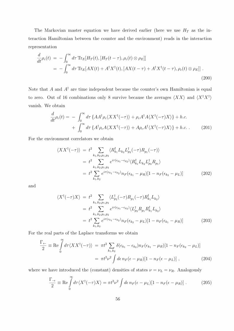
The Markovian master equation we have derived earlier (here we use HT as the in-
teraction Hamiltonian between the counter and the environment) reads in the interaction
representation
d
dtρc(t) = −
∫ ∞0
dτ TrE[HT (t), [HT (t− τ), ρc(t)⊗ ρE]]
= −∫ ∞
0dτ TrE[AX(t) + A†X†(t), [AX(t− τ) + A†X†(t− τ), ρc(t)⊗ ρE]] .
(200)
Note that A and A† are time independent because the counter’s own Hamiltonian is equal
to zero. Out of 16 combinations only 8 survive because the averages 〈XX〉 and 〈X†X†〉vanish. We obtain
d
dtρc(t) = −
∫ ∞0
dτ AA†ρc〈XX†(−τ)〉+ ρcA†A〈X†(−τ)X〉+ h.c.
+∫ ∞
0dτ A†ρcA〈XX†(−τ)〉+ AρcA
†〈X†(−τ)X〉+ h.c. . (201)
For the environment correlators we obtain
〈XX†(−τ)〉 = t2∑
k1,k2,p1,p2
〈R†k1Lk2
L†p2(−τ)Rp1
(−τ)〉
= t2∑
k1,k2,p1,p2
eiτ(εp1−εp2 )〈R†k1Lk2
L†p2Rp1〉
= t2∑k1,k2
eiτ(εk1−εk2
)nF (εk1 − µR)[1− nF (εk2 − µL)] (202)
and
〈X†(−τ)X〉 = t2∑
k1,k2,p1,p2
〈L†p2(−τ)Rp1
(−τ)R†k1Lk2〉
= t2∑
k1,k2,p1,p2
eiτ(εp1−εp2 )〈L†p2Rp1
R†k1Lk2〉
= t2∑k1,k2
eiτ(εk1−εk2
)nF (εk2 − µL)[1− nF (εk1 − µR)] (203)
For the real parts of the Laplace transforms we obtain
Γ←2≡ Re
∞∫0
dτ〈XX†(−τ)〉 = πt2∑k1,k2
δ(εk1 − εk2)nF (εk1 − µR)[1− nF (εk2 − µL)]
= πt2ν2∫dε nF (ε− µR)[1− nF (ε− µL)] , (204)
where we have introduced the (constant) densities of states ν = νL = νR. Analogously
Γ→2≡ Re
∞∫0
dτ〈X†(−τ)X〉 = πt2ν2∫dε nF (ε− µL)[1− nF (ε− µR)] . (205)
56

The combination GT ≡ (2π)× 2πt2ν2 is called the dimensionless tunneling conductance.
At T = 0 and for µL > µR we have hΓ→ = GT2π
(µL − µR), while Γ← = 0.
We obtain for the master equation taking into account that A†A = AA† = 1
d
dtρc(t) = −(Γ← + Γ→)ρc + Γ←A
†ρcA+ Γ→AρcA† . (206)
The density matrix ρc(m1,m2) can in principle have non-diagonal elements. However,
as can be seen from (206), if initially only diagonal elements were present, no off-diagonal
elements would be generated. We assume this situation, which allows us to consider the
charge that has tunneled classically and m becomes a classical ”pointer”. Namely we assume
that at t = 0 the density matrix is given by ρc(t = 0) = δm1,m2 δm1,0 (no charge has tunneled
yet). Then, p(m, t) ≡ ρc(m,m, t) is the probability that m charges have tunneled through.
We obtaind
dtp(m) = −(Γ← + Γ→)p(m) + Γ←p(m+ 1) + Γ→p(m− 1) . (207)
This equation is solved by a Fourier transform introducing the FCS generating function
χ(λ) =∑m p(m)e−iλm. We obtain
d
dtχ(λ) = −(Γ← + Γ→)χ(λ) + eiλΓ←χ(λ) + e−iλΓ→χ(λ)
=[Γ←(eiλ − 1) + Γ→(e−iλ − 1)
]χ(λ) . (208)
Taking into account the initial condition χ(λ, t = 0) = 1 we obtain
χ = et[Γ←(eiλ−1)+Γ→(e−iλ−1)] . (209)
Having the generating function we can calculate, e.g., the total tunneled charge
〈m〉 =∑m
mp(m) = i∂
∂λχ(λ, t)
∣∣∣λ=0
= t(Γ→ − Γ←) . (210)
The average current is clearly given by 〈I〉 = e〈m〉/t = e(Γ→ − Γ←). As we have seen (at
T = 0) we obtain I = eΓ→ = eGT2πh
(µL − µR) = e2GT2πh
V . The tunnel conductance is given by
R−1T = GT
e2
h.
4. Exercise
We consider a qubit which is described by the Hamiltonian HS = −12εσz, where the
states |0〉 = |↑〉 and |1〉 = |↓〉 correspond to two positions of a charged particle. Imagine,
57

e.g., a double-well potential where a single electron is trapped. To describe the tunneling
between the two minima we would have to include a term −12∆σx. We assume here no
tunneling, ∆ = 0, in order to have a QND measurement. The tunneling amplitude of (194)
is now replaced by t → t0 + t1σz, with |t1| < |t0|. Now two different tunneling amplitudes
correspond to states |↑〉 and |↓〉. The new tunneling Hamiltonian reads
HT =∑k1,k2
(t0 + t1σz)[R†k1
Lk2+ L†k2
Rk1
]. (211)
The task is to find the reduced density matrix of the qubit and the counter after tracing out
the microscopic degrees of freedom (electrons), ρ(m1,m2, σ1, σ2).
X. JOSEPHSON QUBITS
A. Elements of BCS theory (only main results shown in the lecture without deriva-
tions)
Our purpose now is to get a bit of BCS theory in order to understand better the Josephson
effect. The derivations a provided in the script but will not be shown in the lecture.
1. BCS Hamiltonian
Everything is done in the grand canonical ensemble. The grand canonical partition
function
ZΩ =∑n,N
e−β(En,N−µN) (212)
shows that at T = 0 one has to minimize HG = H − µN and at T > 0 one has to minimize
Ω = 〈H〉 − TS − µN .
One considers attraction between electrons due to the longitudinal acoustic phonons. The
Hamiltonian reads
HG =∑k,σ
(εk − µ)c†k,σ ck,σ −1
2
g
V
∑k1,σ1,k2,σ2,q
c†k1+q,σ1c†k2−q,σ2
ck2,σ2 ck1,σ2 (213)
where the interaction term works only if the energy transfer εk1+q − εk1 is smaller than the
Debye energy hωD.
58

Although the Hamiltonian conserves the number of particles, BCS (J. Bardeen, L. Cooper,
and R. Schrieffer, 1957) constructed a trial wave function which is a superposition of different
numbers of particles:
|BCS〉 =∏k
(uk + vkc†k,↑c†−k,↓) |0〉 . (214)
with the purpose to use uk and vk as variational parameters and minimize 〈BCS|HG |BCS〉.For this purpose one can introduce a reduced BSC Hamiltonian. In this Hamiltonian only
those terms are left that contribute to the average 〈BCS|HG |BCS〉. The reduced Hamil-
tonian is the one in which k1 = −k2 and σ1 = −σ2:
HBCS =∑k,σ
(εk − µ)c†k,σ ck,σ −1
2
g
V
∑k,q,σ
c†k+q,σ c†−k−q,−σ c−k,−σ ck,σ . (215)
Renaming k′ = k + q we obtain
HBCS =∑k,σ
(εk − µ)c†k,σ ck,σ −1
2
g
V
∑k,k′,σ
c†k′,σ c†−k′,−σ c−k,−σ ck,σ , (216)
or
HBCS =∑k,σ
(εk − µ)c†k,σ ck,σ −g
V
∑k,k′
c†k′,↑ c†−k′,↓ c−k,↓ ck,↑ , (217)
Also the condition on k and k′ gets simplified. We just demand that
µ− hωD < εk, εk′ < µ+ hωD . (218)
2. Variational procedure
Normalization:
1 = 〈BCS| |BCS〉 = 〈0|∏k2
(u∗k2+ v∗k2
c−k2,↓ck2,↑)∏k1
(uk1 + vk1c†k1,↑c
†−k1,↓) |0〉
=∏k
(|uk|2 + |vk|2) . (219)
We further restrict ourselves to real uk and vk such that u2k + v2
k = 1. Thus only one of
them is independent. The following parametrization is helpful: uk = cosφk, vk = sinφk. We
obtain
〈BCS| c†k,↑ ck,↑ |BCS〉
= 〈0|∏k2
(uk2 + vk2c−k2,↓ck2,↑)c†k,↑ ck,↑
∏k1
(uk1 + vk1c†k1,↑c
†−k1,↓) |0〉
= v2k (220)
59
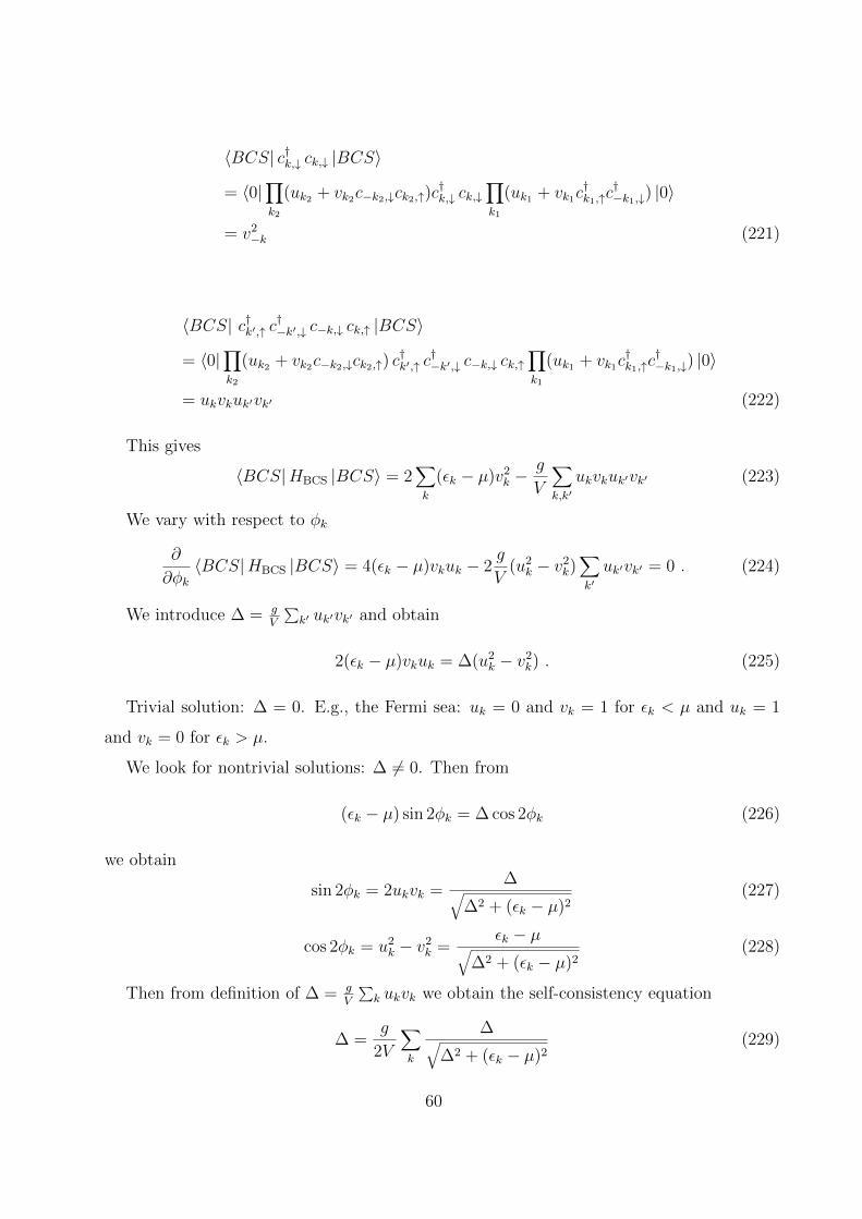
〈BCS| c†k,↓ ck,↓ |BCS〉
= 〈0|∏k2
(uk2 + vk2c−k2,↓ck2,↑)c†k,↓ ck,↓
∏k1
(uk1 + vk1c†k1,↑c
†−k1,↓) |0〉
= v2−k (221)
〈BCS| c†k′,↑ c†−k′,↓ c−k,↓ ck,↑ |BCS〉
= 〈0|∏k2
(uk2 + vk2c−k2,↓ck2,↑) c†k′,↑ c
†−k′,↓ c−k,↓ ck,↑
∏k1
(uk1 + vk1c†k1,↑c
†−k1,↓) |0〉
= ukvkuk′vk′ (222)
This gives
〈BCS|HBCS |BCS〉 = 2∑k
(εk − µ)v2k −
g
V
∑k,k′
ukvkuk′vk′ (223)
We vary with respect to φk
∂
∂φk〈BCS|HBCS |BCS〉 = 4(εk − µ)vkuk − 2
g
V(u2
k − v2k)∑k′uk′vk′ = 0 . (224)
We introduce ∆ = gV
∑k′ uk′vk′ and obtain
2(εk − µ)vkuk = ∆(u2k − v2
k) . (225)
Trivial solution: ∆ = 0. E.g., the Fermi sea: uk = 0 and vk = 1 for εk < µ and uk = 1
and vk = 0 for εk > µ.
We look for nontrivial solutions: ∆ 6= 0. Then from
(εk − µ) sin 2φk = ∆ cos 2φk (226)
we obtain
sin 2φk = 2ukvk =∆√
∆2 + (εk − µ)2(227)
cos 2φk = u2k − v2
k =εk − µ√
∆2 + (εk − µ)2(228)
Then from definition of ∆ = gV
∑k ukvk we obtain the self-consistency equation
∆ =g
2V
∑k
∆√∆2 + (εk − µ)2
(229)
60

or
1 =g
2V
∑k
1√∆2 + (εk − µ)2
=gν0
2
hωD∫−hωD
dξ1√
∆2 + ξ2
= gν0
hωD/∆∫0
dx1√
1 + x2= gν0 ln(
√1 + x2 + x)
∣∣∣hωD/∆0
≈ gν0 ln2hωD
∆(230)
We have assumed ∆ hωD. This gives
∆ = 2hωDe− 1ν0g (231)
We want to convince ourselves that the total energy of the new state is smaller that the
energy of the trivial solution (fully filled Fermi sphere).
EBCS = 〈BCS|HBCS |BCS〉 = 2∑k
(εk − µ)v2k −
g
V
∑k,k′
ukvkuk′vk′
= 2∑k
(εk − µ)v2k −∆
∑k
ukvk , (232)
whereas
ENorm = 〈Norm|HBCS |Norm〉 = 2∑k
(εk − µ)θ(µ− εk) . (233)
We obtain
∆E = EBCS − ENorm = 2∑k
(εk − µ)(v2k − θ(µ− εk))−∆
∑k
ukvk , (234)
With ξk = εk − µ,
v2k = sin2 φk =
1− cos 2φk2
=1
2− ξk
2√
∆2 + ξ2k
(235)
and
ukvk =∆
2√
∆2 + ξ2k
(236)
we obtain
∆E =∑k
2ξk
1
2− ξk
2√
∆2 + ξ2k
− θ(−ξk)− ∆2
2√
∆2 + ξ2k
(237)
∆E = 2V
hωD∫0
ν0dξ
(ξ
[1
2− ξ
2√
∆2 + ξ2− θ(−ξ)
]− ∆2
2√
∆2 + ξ2
)
= 2V
hωD∫0
ν0dξ
ξ − ξ2
√∆2 + ξ2
− ∆2
2√
∆2 + ξ2k
= 2V ν0∆2
hωD/∆∫0
dx
(x−√
1 + x2 +1
2√
1 + x2
)(238)
61

The last integral is convergent and for hωD ∆ can be taken to ∞. The integral gives
−1/4. Thus
∆E = −V ν0∆2
2. (239)
Roughly energy ∆ per electron in window of energies of order ∆.
3. Excitations
We want to consider the BCS ground state as vacuum and find the quasiparticle excita-
tions above it. Let us start with the normal state, i.e., vk = θ(−ξk) and uk = θ(ξk). For
ξk > 0 we have
ck,σ |Norm〉 = 0 (240)
while for ξk < 0
c†k,σ |Norm〉 = 0 (241)
we introduce
αk,σ ≡
ck,σ if ξk < 0
±c†−k,−σ if ξk > 0(242)
or equivalently
αk,σ = ukck,σ ± vkc†−k,−σ (243)
(the sign to be chosen). We see, thus, that αk,σ |Norm〉 = 0, whereas
α†k,σ = ukc†k,σ ± vkc−k,−σ (244)
creates an excitation of energy |ξk|. For the BCS state we obtain
αk,σ |BCS〉 = (ukck,σ ± vkc†−k,−σ)∏q
(uq + vqc†q,↑c†−q,↓) |0〉 (245)
We see that the proper choice of sign is
αk,σ = ukck,σ − σvkc†−k,−σ (246)
and
αk,σ |BCS〉 = 0 . (247)
The conjugated (creation) operator reads
α†k,σ = ukc†k,σ − σvkc−k,−σ (248)
62

One can check the commutation relations
αk,σ, α
†k′,σ′
+
= δk,k′δσ,σ′ (249)
αk,σ, αk′,σ′+ = 0α†k,σ, α
†k′,σ′
+
= 0 (250)
The inverse relations read:
ck,σ = ukαk,σ + σvkα†−k,−σ , c†k,σ = ukα
†k,σ + σvkα−k,−σ (251)
4. Mean field
We adopt the mean field approximation for the BCS Hamiltonian.
HBCS =∑k,σ
(εk − µ)c†k,σ ck,σ −g
V
∑k,k′
c†k′,↑ c†−k′,↓ c−k,↓ ck,↑ . (252)
Note that in the interaction the terms with k = k′ are absent, since the matrix element of
the electron-phonon interaction is proportional to the momentum transfer q = k− k′. Thus
the only averages we can extract in the interaction term are 〈c−k,↓ ck,↑〉 and 〈c†k,↑ c†−k,↓〉. We
use
c†k,↑ c†−k,↓ = (ukα
†k,↑ + vkα−k,↓)(ukα
†−k,↓ − vkαk,↑)
= u2kα†k,↑α
†−k,↓ − v2
kα−k,↓αk,↑ + ukvk(1− α†k,↑αk,↑ − α†−k,↓α−k,↓) . (253)
and
c−k,↓ck,↑ = u2kα−k,↓αk,↑ − v2
kα†k,↑α
†−k,↓ + ukvk(1− α†k,↑αk,↑ − α†−k,↓α−k,↓) . (254)
In the BCS ground state we obtain 〈c−k,↓ ck,↑〉 = vkuk and 〈c†k,↑ c†−k,↓〉 = vkuk. We use
AB = 〈A〉 〈B〉+ 〈A〉 (B − 〈B〉) + (A− 〈A〉) 〈B〉+ (A− 〈A〉)(B − 〈A〉)
and neglect the last term. The mean field Hamiltonian reads
HMFBCS =
∑k,σ
(εk − µ)c†k,σ ck,σ +g
V
∑k,k′〈c†k′,↑ c†−k′,↓〉 〈c−k,↓ ck,↑〉
− g
V
∑k,k′〈c†k′,↑ c†−k′,↓〉 c−k,↓ ck,↑ −
g
V
∑k,k′
c†k′,↑ c†−k′,↓ 〈c−k,↓ ck,↑〉
=∑k,σ
ξkc†k,σ ck,σ −
∑k
∆c−k,↓ ck,↑ −∑k
∆c†k,↑ c†−k,↓ + V
∆2
g(255)
63

Substituting the expressions for c operators in terms of α operators we obtain a diagonal
Hamiltonian (exercise)
H =∑k,σ
Ekα†k,σ αk,σ + const. , (256)
where Ek =√
∆2 + ξ2k. For proof one needs
c†k,↑ ck,↑ + c†−k,↓ c−k,↓ = (ukα†k,↑ + vkα−k,↓)(ukαk,↑ + vkα
†−k,↓)
+(ukα†−k,↓ − vkαk,↑)(ukα−k,↓ − vkα†k,↑)
= (u2k − v2
k)(α†k,↑αk,↑ + α†−k,↓α−k,↓) + 2v2
k + 2ukvk(α†k,↑α
†−k,↓ + α−k,↓αk,↑) (257)
5. Order parameter, phase
Thus far ∆ was real. We could however introduce a different BCS groundstate:
|BCS(φ)〉 =∏k
(uk + eiφvkc†k,↑c†−k,↓) |0〉 . (258)
Exercise: check that
|BCS(N)〉 =
2π∫0
dφ
2π|BCS(φ)〉 e−iNφ (259)
gives a state with a fixed number of electrons N . We obtain for ∆
∆ =g
V
∑k
〈c−k,↓ck,↑ 〉 =g
V
∑k
ukvkeiφ = |∆|eiφ (260)
It is easy to see that the operator A† = e−iφ increases the number of Cooper pairs by one
A† |BCS(N)〉 =
2π∫0
dφ
2π|BCS(φ)〉 e−i(N+1)φ = |BCS(N + 1)〉 . (261)
We have seen that the excitations above the BCS ground state have an energy gap ∆.
Thus, if T ∆ no excitations are possible. The only degree of freedom left is the pair of
conjugate variables N, φ with commutation relations [N, e−iφ] = e−iφ. Indeed the ground
state energy is independent of φ. This degree of freedom is, of course, non-existent if the
number of particles is fixed. Thus a phase of an isolated piece of a superconductor is quantum
mechanically smeared between 0 and 2π and no dynamics of the degree of freedom N, φ is
possible. However in a bulk superconductor the phase can be space dependent φ(~r). One can
still add a constant phase to φ(~r) +φ0 without changing the state. More precisely the phase
64

φ0 is smeared if the total number of particles is fixed. However the difference of phases, i.e.,
the phase gradient can be well defined and corresponds to a super-current.
We have to consider the gauge invariance. The usual gauge transformation reads
~A→ ~A+ ~∇χ , (262)
Ψ→ Ψeiehcχ , (263)
where Ψ is the electron wave function (field). Comparing with (258) we see that adding
phase φ corresponds to a transformation c†k,σ → eiφ/2c†k,σ. This we identify
φ
2= − e
hcχ . (264)
Thus
~A→ ~A− hc
2e~∇φ (265)
We postulate here the gauge invariant form of the London equation
~js = −e2nsmc
(~A− hc
2e~∇φ), (266)
where ns is the density of superconducting electrons. At T = 0 all electrons are super-
conducting, thus ns = n. We do not derive this relation here, but we do so later for the
tunneling current between two superconductors with a phase difference between them.
6. Flux quantization
In the bulk of a superconductor, where ~js = 0, we obtain
~A− hc
2e~∇φ = 0 (267)
∮~Ad~l =
hc
2e
∮~∇φd~l =
hc
2e2πn =
hc
2en = nΦ0 (268)
This quantization is very important for, e.g., a ring geometry. If the ring is thick enough
(thicker than λL) the total magnetic flux threading the ring is quantized.
65

B. Josephson effect
We consider now a tunnel junction between two superconductors with different phases
φL and φR. The Hamiltonian reads
H = HBCS,L +HBCS,R +HT , (269)
where analogously to (194) we write
HT =∑
k1,k2,σ
T[R†k1,σ
Lk2,σ+ L†k2,σ
Rk1,σ
]. (270)
Here Rk,σ ≡ c(R)k,σ is the annihilation operator of an electron in the left superconductor. Two
important things: 1) microscopically the electrons and not the quasiparticles tunnel; 2)
tunneling conserves spin.
A gauge transformation Lk,σ → eiφL/2Lk,σ and Rk,σ → eiφR/2Rk,σ ”removes” the phases
from the respective BCS wave functions (making vk, uk, and ∆ real) and renders the tun-
neling Hamiltonian
HT =∑
k1,k2,σ
T[R†k1,σ
Lk2,σe−iφ/2 + L†k2,σ
Rk1,σeiφ/2
], (271)
where φ ≡ φR − φL. Note the similarity with the Full Counting Statistics.
Josephson [5] used (271) and calculated the tunneling current. We do so here for a time-
independent phase difference φ. The current operator is given by time derivative of the
number of particles in the right lead NR =∑k,σ R
†k,σRk,σ
I = −eNR = −ieh
[HT , NR] =ie
h
∑k1,k2,σ
T[R†k1,σ
Lk2,σe−iφ/2 − L†k2,σ
Rk1,σeiφ/2
]. (272)
The first order time-dependent perturbation theory gives for the density matrix of the system
in the interaction representation
ρ(t) = Te−i∫ t−∞ dt′HT (t′)
ρ0T ei∫ t−∞ dt′HT (t′) ≈ −i
∫ t
−∞dt′[HT (t′), ρ0] . (273)
For the expectation value of the current this gives
〈I(t)〉 = Trρ(t)I(t) = −i∫ t
−∞dt′Tr [HT (t′), ρ0]I(t) = −i
∫ t
−∞dt′Tr [I(t), HT (t′)] ρ0 .
(274)
66

We use
〈BCS| c†k,↑(t1) c†−k,↓(t2) |BCS〉
= 〈BCS|(ukα
†k,↑(t1) + vkα−k,↓(t1)
) (ukα
†−k,↓(t2)− vkαk,↑(t2)
)|BCS〉
= vkuke−iEk(t1−t2) , (275)
and
〈BCS| ck,↑(t1) c−k,↓(t2) |BCS〉
= 〈BCS|(ukαk,↑(t1) + vkα
†−k,↓(t1)
) (ukα−k,↓(t2)− vkα†k,↑(t2)
)|BCS〉
= −vkuke−iEk(t1−t2) , (276)
After some algebra we obtain (from the anomalous correlators, the rest gives zero)
〈I(t)〉 = − 2eT 2e−iφ∫ t
−∞dt′
∑k1,k2
vk1uk1vk2uk2
[e−i(Ek1
+Ek2)(t−t′) − ei(Ek1
+Ek2)(t−t′)
]+ 2eT 2eiφ
∫ t
−∞dt′
∑k1,k2
vk1uk1vk2uk2
[e−i(Ek1
+Ek2)(t−t′) − ei(Ek1
+Ek2)(t−t′)
]
= 8eT 2 sin(φ)∑k1,k2
vk1uk1vk2uk2
Ek1 + Ek2
= 2eT 2 sin(φ)∑k1,k2
∆2
Ek1Ek2(Ek1 + Ek2)
= 2π2T 2ν2e∆h−1 sin(φ) = Ic sin(φ) , (277)
where the Josephson critical current is given by
Ic =gT e∆
4h=
π∆
2eRT
, (278)
where gT = 2 × 4π2T 2ν2 is the dimensionless conductance of the tunnel junction (factor 2
accounts for spin), while the tunnel resistance is given by RT = he2
1gT
. This is the famous
Ambegaokar-Baratoff relation [6] (see also erratum [7]).
Thus we have obtained the first Josephson relation I = Ic sinφ. We have introduced the
variable φ as the difference of two phases φ = φR−φL. The gauge invariant definition reads
φ = φR − φL −2e
hc
∫ R
L
~Ad~l . (279)
As a shortest way to the second Josephson relation we assume that an electric field exists
in the junction and that it is only due to the time-dependence of ~A. Then we obtain
φ = −2e
hc
∫ R
L
[∂
∂t~A
]d~l =
2e
h
∫ R
L
~Ed~l = −2e
hV , (280)
67

where V is the voltage. Here we all the time treated e as the charge of the electron, i.e.,
e < 0. Usually one uses e as a positive quantity. Then
φ =2eV
h. (281)
An alternative way to derive this is to start with a difference of (time-dependent) chemical
potentials
H = HL +HR − eVL(t)∑k,σ
L†k,σLk,σ − eVR(t)∑k,σ
R†k,σRk,σ +HT , (282)
where VL/R are the applied electro-chemical potentials (in addition to the constant chemical
potential µ, which is included in HL and HR). A transformation with
U = eehNL
t∫VL(t′)dt′ e
ehNR
t∫VR(t′)dt′ (283)
In the new Hamiltonian
H = iUU−1 + UHU−1 . (284)
the terms with VL and VR are cancelled and instead the electronic operators are replaced
by, e.g,
L→ ULU−1 = LeiφL/2 , (285)
where φL = const.− 2eh
t∫VL(t′)dt′ and, thus, φ = φR − φL = −2e
hV .
C. Macroscopic quantum phenomena
1. Resistively shunted Josephson junction (RSJ) circuit
Consider a circuit of parallelly connected Josephson junction and a shunt resistor R. A
Josephson junction is simultaneously a capacitor. An external current Iex is applied. The
Kirchhoff rules lead to the ecquation
Ic sinφ+V
R+ Q = Iex . (286)
As Q = CV and V = h2eφ. Thus we obtain
Ic sinφ+h
2eRφ+
hC
2eφ = Iex . (287)
68

Iex
C
R
Ic
FIG. 22: RSJ Circuit.
It is very convenient to measure the phase in units of magnetic flux, so that V = 1cΦ (in SI
units V = Φ):
Φ =ch
2eφ =
Φ0
2πφ , φ = 2π
Φ
Φ0
. (288)
Then the Kirchhoff equation reads
Ic sin(
2πΦ
Φ0
)+
Φ
cR+CΦ
c= Iex , (289)
or in SI units
Ic sin(
2πΦ
Φ0
)+
Φ
R+ CΦ = Iex . (290)
There are two regimes. In case Iex < Ic there exists a stationary solution φ = arcsin(Iex/Ic).
All the current flows through the Josephson contact as a super-current. Indeed V ∝ φ = 0.
At Iex > Ic at least part of the current must flow through the resistor. Thus a voltage
develops and the phase starts to ”run”.
2. Particle in a washboard potential
The equation of motion (290) can be considered as an equation of motion of a particle
with the coordinate x = Φ. We must identify the capacitance with the mass, m = C, the
inverse resistance with the friction coefficient γ = R−1. Then we have
mx = −γx− ∂U
∂x, (291)
69

Φ
U(Φ)
FIG. 23: Washboard potential.
FIG. 24: Macroscopic Quantum Tunneling (MQT).
where for the potential we obtain
U(Φ) = −EJ cos(
2πΦ
Φ0
)− IexΦ , (292)
where
EJ ≡IcΦ0
2π=hIc2e
(293)
is called the Josephson energy. The potential energy U(Φ) has a form of a washboard and
is called a washboard potential. In Fig. 23 the case Iex < Ic is shown. In this case the
potential has minima and, thus, classically stationary solutions are possible.
When the external current is close to the critical value a situation shown in Fig. 24
emerges. If we allow ourselves to think of this situation quantum mechanically, then we would
conclude that only a few quantum levels should remain in the potential well. Moreover a
tunneling process out of the well should become possible. This tunneling process was named
70

Macroscopic Quantum Tunneling because in the 80-s and the 90-s many researchers doubted
the fact one can apply quantum mechanics to the dynamics of the ”macroscopic” variable
Φ. It was also argued that a macroscopic variable is necessarily coupled to a dissipative
bath which would hinder the tunneling. Out these discussions the famous Caldeira-Leggett
model emerged [8, 9].
3. Quantization
We write down the Lagrangian that would give the equation of motion (291 or 290).
Clearly we cannot include the dissipative part in the Lagrange formalism. Thus we start
from the limit R→∞. The Lagrangian reads
L =CΦ2
2− U(Φ) =
CΦ2
2+ EJ cos
(2π
Φ
Φ0
)+ IexΦ . (294)
We transform to the Hamiltonian formalism and introduce the canonical momentum
Q ≡ ∂L
∂Φ= CΦ . (295)
The Hamiltonian reads
H =Q2
2C+ U(Φ) =
Q2
2C− EJ cos
(2π
Φ
Φ0
)− IexΦ . (296)
The canonical momentum corresponds to the charge on the capacitor (junction). The usual
commutation relations should be applied
[Φ, Q] = ih . (297)
In the Hamilton formalism it is inconvenient to have an unbounded from below potential.
Thus we try to transform the term −IexΦ away. This can be achieved by the following
canonical transformation
R = exp[− ihQex(t)Φ
], (298)
where Qex(t) ≡t∫Iex(t
′)dt′. Indeed the new Hamiltonian reads
H = RHR−1 + ihRR−1 =(Q−Qex(t))
2
2C− EJ cos
(2π
Φ
Φ0
). (299)
71

The price we pay is that the new Hamiltonian is time-dependent. The Hamiltonian (299) is
very interesting. Let us investigate the operator
cos(
2πΦ
Φ0
)= cos
(2e
hΦ)
=1
2exp
[i
h2eΦ
]+ h.c. (300)
We have
exp[i
h2eΦ
]|Q〉 = |Q+ 2e〉 , exp
[− ih
2eΦ]|Q〉 = |Q− 2e〉 . (301)
Thus in this Hamiltonian only the states differing by an integer number of Cooper pairs
get connected. The constant offset charge remains undetermined. This, however, can be
absorbed into the bias charge Qex. Thus, we can restrict ourselves to the Hilbert space
|Q = 2em〉.
4. Josephson energy dominated regime
In this regime EJ EC , where EC = (2e)2
2Cis the Cooper pair charging energy. Let us first
neglect EC completely, i.e., put C =∞. Recall that C plays the role of the mass. Then the
Hamiltonian reads H = −EJ cos(2πΦ
Φ0
). On one hand it is clear that the relevant state are
those with a given phase, i.e., |Φ〉. On the other hand, in the discrete charge representation
the Hamiltonian reads
H = −EJ2
∑m
(|m+ 1〉 〈m|+ |m〉 〈m+ 1|) . (302)
The eigenstates of this tight-binding Hamiltonian are the Bloch waves |k〉 =∑m e
ikm |m〉with the wave vector k belonging to the first Brillouin zone −π ≤ k ≤ π. The eigenenergy
reads Ek = −EJ cos(k). Thus we identify k = φ = 2πΦΦ0
.
5. Charging energy dominated regime
In this regime EJ EC . The main term in the Hamiltonian is the charging energy term
HC =(Q−Qex(t))
2
2C=
(2em−Qex)2
2C. (303)
The eigenenergies corresponding to different values of m form parabolas as functions of
Qex (see Fig. 25). The minima of the parabolas are at Qex = 0, 2e, 4e, . . .. The Josephson
72

energies
Q=0 Q=2e Q=4e
eigen
Qexe 2e 3e0 4e
FIG. 25: Eigen levels in the coulomb blockade regime. Different parabolas correspond to different
values of Q = 2em. The red lines represent the eigenlevels with the Josephson energy taken into
account. The Josephson tunneling lifts the degeneracy between the charge states.
tunneling term serves now as a perturbation HJ = −EJ cos(2πΦ
Φ0
). It lifts the degeneracies,
e.g., at Qex = e, 3e, 5e, . . ..
If a small enough external current is applied, Qex = Iext the adiabatic theorem holds and
the system remains in the ground state. Yet, one can see that between the degeneracies
at Qex = e, 3e, 5e, . . . the capacitance is charged and discharged and oscillating voltage
V = ∂E0/∂Qex appears. Here E0(Qex) is the energy of the ground state. The Cooper pairs
tunnel only at the degeneracy points. In between the Coulomb blockade prevents the Cooper
pairs from tunneling because this would cost energy.
6. Caldeira-Leggett model
In order to describe the dissipation due to the shunt resistor a bath of linear oscillators
is added. The Hamiltonian now reads
H =Q2
2C+ U(Φ) +
∑n
p2n
2mn
+mnω
2n
(xn − λn
mnω2nΦ)2
2
. (304)
Equations of motion:
Φ =∂H
∂Q=Q
C,
Q = −∂H∂Φ
= −∂U∂Φ
+∑n
λn
(xn −
λnmnω2
n
Φ
),
73

xn =∂H
∂pn=
pnmn
,
pn = − ∂H∂xn
= −mnω2n
(xn −
λnmnω2
n
Φ
). (305)
This gives
CΦ = −∂U∂Φ
+∑n
λnxn − Φ∑n
λ2n
mnω2n
,
mnxn +mnω2nxn = λnΦ . (306)
The second equation is solved by the Fourier transform. We obtain
xn(t) =∫dt′αn(t− t′)Φ(t′) + x(free)
n (t), (307)
where
αn(ω) =λn
mn(ω2n − (ω + iδ)2)
. (308)
The sign of the iδ term is chosen to make αn retarded, i.e., αn(τ < 0) = 0. We obtain
∑n
λnxn(t) =∫dt′α(t− t′)Φ(t′) + ξ(t) , (309)
where
α(ω) =∑n
λ2n
mn(ω2n − (ω + iδ)2)
(310)
and
ξ(t) =∑n
λnx(free)n (t) . (311)
We introduce the spectral density
J(ν) ≡ π
2
∑n
λ2n
mnωnδ(ν − ωn) . (312)
This gives
α(ω) =2
π
∫dν
νJ(ν)
ν2 − (ω + iδ)2(313)
and, finally,
Imα(ω) = α′′(ω) =
J(ω) for ω > 0
−J(−ω) for ω < 0. (314)
An Ohmic bath is defined by
J(ω) = R−1ω , (315)
74

ΦJ
Vg
Φg
E J , C J C g
FIG. 26: Cooper Pair Box. The Josephson tunnel junction is characterized by the Josephson energy
EJ and by the capacitance CJ . The superconducting island is controlled by the gate voltage Vg
via the gate capacitance Cg. To derive the system’s Lagrangian and Hamiltonian we introduce the
phase drop on the Josephson junction ΦJ and the phase drop on the gate capacitor Φg.
up to some cutoff frequency ωc. We disregard, first, Reα(ω) = α′(ω) and obtain
α′′(t− t′) =∫ dω
2πe−iω(t−t′)iR−1ω = R−1 ∂
∂t′δ(t− t′) (316)
Thus ∫dt′α′′(t− t′)Φ(t′) = −R−1Φ(t) . (317)
The equation of motion now reads
CΦ = −∂U∂Φ− Φ
R− Φ
∑n
λ2n
mnω2n
+∫dt′α′(t− t′)Φ(t′) + ξ(t) (318)
The second term of the RHS is the friction force due to the oscillators (resistor). The third
and the fourth terms represent the renormalization of U(Φ). Our choice of coupling to the
oscillators was such that these two terms mostly cancel each other. Finally, the last term
of the RHS is the Langevin random force. We see that this is due to the free motion of the
oscillators.
D. Various qubits
1. Charge qubit
We start by considering the so called Cooper pair box shown in Fig. 26. We derive the
Hamiltonian starting from the Lagrangian
L =CJΦ2
J
2+CgΦ
2g
2− UJ(ΦJ) , (319)
75

where UJ = −EJ cos(2π ΦJ
Φ0
). The sum of all the phases along the loop must vanish and the
phase on the voltage source is given by const.+ Vgt. Thus we obtain
Φg = −ΦJ − Vg (320)
and the Lagrangian in terms of the only generalized coordinate ΦJ reads
L =CJΦ2
J
2+Cg(ΦJ + Vg)
2
2− UJ(ΦJ)
=(CJ + Cg)Φ
2J
2+ CgΦJVg − UJ(ΦJ) + const. . (321)
The conjugated momentum (charge) reads
Q =∂L
∂ΦJ
= (CJ + Cg)ΦJ + CgVg . (322)
Since CJΦJ is the charge on the Josephson junction capacitance while CgΦJ+CgVg = −CgΦg
is minus the charge on the gate capacitance we conclude that Q = 2em is the charge on the
island (we disregard here the possibility to have an odd number of electrons on the island).
We obtain
ΦJ =Q− CgVgCJ + Cg
. (323)
The Hamiltonian reads
H = Q ΦJ − L =(Q− CgVg)2
2(CJ + Cg)+ UJ(ΦJ)
=(Q− CgVg)2
2(CJ + Cg)− EJ cos
(2π
ΦJ
Φ0
). (324)
This is exactly the Hamiltonian (299) with Qex = CgVg. The two level system is formed by
the two lowest levels around CgVg = e+ 2eN .
In Hamiltonian (324) the interplay of two energy scales determines the physical regime.
These are 1) Josephson energy EJ ; 2) Charging energy EC ≡ (2e)2
2(CJ+Cg). In the simplest
regime EJ EC and for Qex ∼ e one can restrict the Hilbert space to two charge states
with lowest charging energies |↑〉 = |Q = 0〉 and |↓〉 = |Q = 2e〉. In this Hilbert space we
have
cos(
2πΦJ
Φ0
)=
1
2σx , (325)
and
Q = e(1− σz) . (326)
76

Φ
E0
J
Vg
x
FIG. 27: Charge quit with controllable Josephson energy.
Substituting these to (324) and disregarding constant energy shifts we obtain
H = −1
2
(1− Qex
e
)EC σz −
1
2EJ σx . (327)
Thus we obtain an effective spin-1/2 in a magnetic field whose z-component can be controlled
by the gate voltage.
In Fig. 27 a charge qubit is shown in which the Josephson junction was replaced by a dc-
SQUID. A straightforward derivation (assuming the geometrical inductance of the SQUID
loop being vanishingly small) gives again the Hamiltonian (324) with CJ → 2CJ (just
because there are two junctions instead of one) and
EJ → 2E(0)J cos
(πΦx
Φ0
). (328)
Here E(0)J is the Josephson energy of a single junction. We assume the two junctions of the
SQUID to be identical. Now we can control also the x-component of the effective magnetic
field.
77

Mirror
Beam splitter Phase shift
Single photonsorce
Photondetector
FIG. 28: The qubit is encoded into the path of a single photon. A 50 % beam splitter represents
a Hadamard gate, while a phase gate is a simple phase shift in one arm of the interferometer.
2. Flux qubit
3. Phase qubit
XI. OPTICAL QUBITS AND CAVITY QED
A. Photons as Qubits
In many ways photons are the perfect qubits. Their polarization is a natural two level
system and one has not to worry about populating higher levels. Alternatively, photons
can travel through a Mach–Zehnder interferometer with two paths and the qubit is encoded
in the “which path” degree of freedom, as depicted in fig. 28. All single qubit transforma-
tions can be easily achieved with mirrors, beam splitters, phase shifts. On demand single
photon generators improve rapidly and single photon detectors for the readout are available
(although so far only with about 60 % efficiency). Photons interact very little with the
78
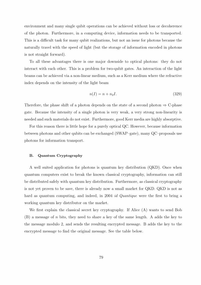
environment and many single qubit operations can be achieved without loss or decoherence
of the photon. Furthermore, in a computing device, information needs to be transported.
This is a difficult task for many qubit realizations, but not an issue for photons because the
naturally travel with the speed of light (but the storage of information encoded in photons
is not straight forward).
To all these advantages there is one major downside to optical photons: they do not
interact with each other. This is a problem for two-qubit gates. An interaction of the light
beams can be achieved via a non-linear medium, such as a Kerr medium where the refractive
index depends on the intensity of the light beam
n(I) = n+ n2I. (329)
Therefore, the phase shift of a photon depends on the state of a second photon ⇒ C-phase
gate. Because the intensity of a single photon is very weak, a very strong non-linearity is
needed and such materials do not exist. Furthermore, good Kerr media are highly absorptive.
For this reason there is little hope for a purely optical QC. However, because information
between photons and other qubits can be exchanged (SWAP–gate), many QC–proposals use
photons for information transport.
B. Quantum Cryptography
A well suited application for photons is quantum key distribution (QKD). Once when
quantum computers exist to break the known classical cryptography, information can still
be distributed safely with quantum key distribution. Furthermore, as classical cryptography
is not yet proven to be save, there is already now a small market for QKD. QKD is not as
hard as quantum computing, and indeed, in 2004 id Quantique were the first to bring a
working quantum key distributor on the market.
We first explain the classical secret key cryptography. If Alice (A) wants to send Bob
(B) a message of n bits, they need to share a key of the same length. A adds the key to
the message modulo 2, and sends the resulting encrypted message. B adds the key to the
encrypted message to find the original message. See the table below.
79

message 0 1 0 0 1 1 0
key 1 1 0 1 0 1 0
encrypted message 1 0 0 1 1 0 0
decrypted message 0 1 0 0 1 1 0
This protocol is perfectly save given that no one else knows the key. Therefore, the
problem of cryptography is reduced to transmitting or sharing a key. Classically, whenever
a key is transmitted, someone else (often called Eve (E)) can intercept the transmission to
gain the key. If the key is encoded into a qubit, then, whenever Eve measures the qubit
to gain the key, she will also change the state of the qubit. Therefore, Alice and Bob can
detect that Eve intercepted the line and not send the message in this case.
There are several protocols for QKD, here we present the simplest BB84 QKD protocol.
For A to transfer a key on length n, she needs 4n qubits which she can prepare in the states
|0〉 , |1〉 , |+〉 = (|0〉 + |1〉)/√
2, and |−〉 = (|0〉 − |1〉)/√
2. The states |0〉 and |+〉 are both
used to encode a 0, while |1〉 and |−〉 encode a 1. Then she generates 4n random numbers
b. Whenever b = 0, then she uses the (0,1) basis to encode bits, while when b = 1 she uses
the (+,−) basis. Next she generates another 4n random numbers a which represent the key
and which she will encode in the basis determined by b.
She now sends the qubits to Bob, who will generate 4n random numbers b′ to determine
in which basis he will measure the qubit. If he measures the states |0〉 or |+〉 he will note a
0, and if he measures |1〉 or |−〉, he will note a 1.
qubit number b a state of qubit b′ a′
1 0 1 |1〉 0 1
2 0 0 |0〉 1 0 or 1
3 1 1 |−〉 0 0 or 1
4 1 1 |−〉 1 1
5 0 1 |1〉 1 0 or 1
6 1 0 |+〉 1 0...
......
......
...
4n 0 0 |0〉 1 0 or 1
80

Once Bob has measured all qubits, he tells Alice in which basis b′ he measured and Alice
tells Bob in which basis b she prepared. This is done using a public line, so Eve is allowed
to get this information. Now they discard all bits where they used different bases, i.e. they
only keep bits with b = b′. For these they know that a = a′ and they now share a key of
length 2n.
Now we assume Eve intercepts the line. Assume A sends |1〉 as in qubit number one. At
this time it is not yet public which basis A used. Therefore E can only choose randomly,
and with probability p1 = 0.5 she chooses the (+−) basis. Now she would ideally send |1〉to B and no one could realized that she intercepted the transmission. However, she does
not know that A send out |1〉. The best she can do is to send out what she measured. If
B measures in the basis (0,1), with probability p2 = 0.5, he will measure 0. Therefore, if E
intercepts, then A and B will have different bits a 6= a′ with probability p = p1p2 = 0.25.
A will now randomly choose n bits which they public compare on a public line. If all n
bits are the same, they can use the other n bits as secret key. If about a quarter of the n
bits are different, then they know that someone intercepted and do not use the key. Note
that E can still prevent A from sending a message to B, but she can do that anyway by
cutting the line. But she can not get the message!
One seemingly obvious way for Eve to stay undetected is to copy the state sent by A,
then forward one copy to B and use the other for her measurements. However, the no
cloning theorem forbids copying of an unknown quantum state. The theorem is easy to
prove by contradiction. To copy a state from system 1 to system 2 means to perform the
transformation |ψ〉1⊗ |0〉2 → |ψ〉1⊗ |ψ〉2. This should be valid for all input states, therefore
|φ〉1 ⊗ |0〉2 → |φ〉1 ⊗ |φ〉2. Every unitary transformation preserves the scalar product, which
leads to 〈φ|ψ〉 = 〈φ|ψ〉2. This is clearly not true for general states. This can easily be
generalized to trace–preserving and completely positive quantum operations.
This protocol is easily performed using the polarization of a photon as qubit. However,
photon detectors are not perfect and Bob will sometimes find the wrong result. Therefore,
if A wants to transmit a 0, she tells Bob a number of qubits which he should have detected
in the state 0. Given that Bob only rarely finds a wrong measurement result, he can use a
majority vote to decide what the bit should be. This is shown below where they use five
81
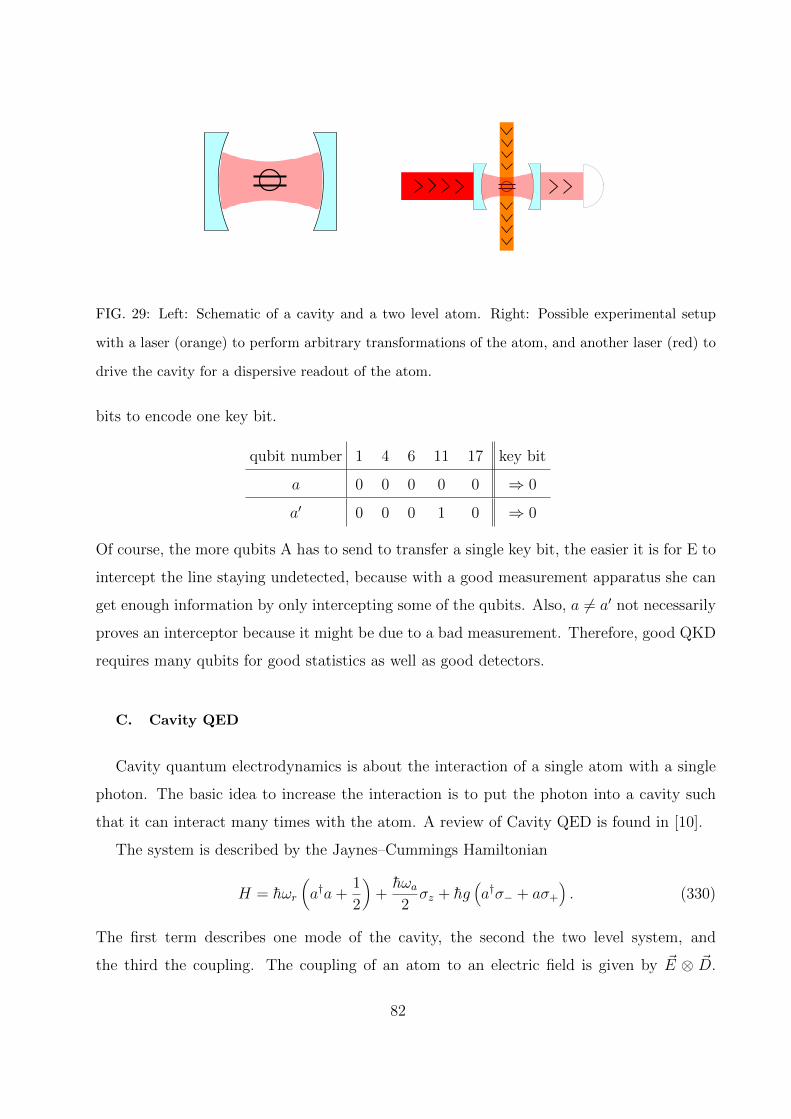
FIG. 29: Left: Schematic of a cavity and a two level atom. Right: Possible experimental setup
with a laser (orange) to perform arbitrary transformations of the atom, and another laser (red) to
drive the cavity for a dispersive readout of the atom.
bits to encode one key bit.
qubit number 1 4 6 11 17 key bit
a 0 0 0 0 0 ⇒ 0
a′ 0 0 0 1 0 ⇒ 0
Of course, the more qubits A has to send to transfer a single key bit, the easier it is for E to
intercept the line staying undetected, because with a good measurement apparatus she can
get enough information by only intercepting some of the qubits. Also, a 6= a′ not necessarily
proves an interceptor because it might be due to a bad measurement. Therefore, good QKD
requires many qubits for good statistics as well as good detectors.
C. Cavity QED
Cavity quantum electrodynamics is about the interaction of a single atom with a single
photon. The basic idea to increase the interaction is to put the photon into a cavity such
that it can interact many times with the atom. A review of Cavity QED is found in [10].
The system is described by the Jaynes–Cummings Hamiltonian
H = hωr
(a†a+
1
2
)+hωa
2σz + hg
(a†σ− + aσ+
). (330)
The first term describes one mode of the cavity, the second the two level system, and
the third the coupling. The coupling of an atom to an electric field is given by ~E ⊗ ~D.
82

While ~E is proportional to (a† + a), the dipole moment of the atom is proportional to
σx = (σ+ + σ−). The two terms which do not conserve the number of excitations can be
neglected in the rotating wave approximation. That can be seen by transforming into the
interaction picture with U = eihωra†a ⊗ eihωaσz/2. The terms which approximately preserve
the energy of the system without interaction oscillate slowly, while the others oscillate fast
and can be neglected. For the same reason other modes of the cavity and other levels of the
atom do not have to be considered.
The regime most interesting is the strong coupling regime g γ, κ, where γ is the rate of
spontaneous emission of the atom, and κ is the loss rate of the cavity. To reach this regime
(which is very difficult) the following things can be done
• Small mode volume: The smaller the cavity, the stronger the electric field of a
single photon. The size of the cavity is limited by the wavelength. Also, κ increases
with the inverse length of the cavity because the photon has to be reflected more often
in the same time interval.
• Rydberg atoms: These are highly excited atoms with the principal quantum number
n of the order of one hundred. They also have a low decay rate, but they are not easy
to prepare with good fidelity.
• Highly reflective mirrors: The best mirrors are superconducting mirrors, but they
can only be used for microwave cavities because shorter wavelength can excite quasi
particles. Also optical mirrors are better for infra red light than for visible or UV light.
Therefore, there is a trade-off with the first item.
We introduce N = a†a+ σz to count the number of excitations. Because [H,N ] = 0, the
number of excitations is preserved. Using the detuning ∆ = ωa − ωr we write
H = ωrN + ∆σz/2 + g(a†σ− + aσ+
). (331)
83
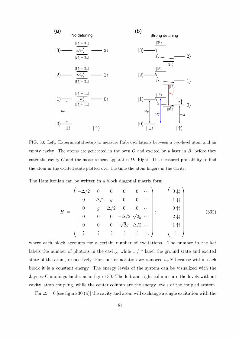
No detuning Strong detuning(a) (b)
FIG. 30: Left: Experimental setup to measure Rabi oscillations between a two-level atom and an
empty cavity. The atoms are generated in the oven O and excited by a laser in B, before they
enter the cavity C and the measurement apparatus D. Right: The measured probability to find
the atom in the excited state plotted over the time the atom lingers in the cavity.
The Hamiltonian can be written in a block diagonal matrix form
H =
−∆/2 0 0 0 0 · · ·0 −∆/2 g 0 0 · · ·0 g ∆/2 0 0 · · ·0 0 0 −∆/2
√2g · · ·
0 0 0√
2g ∆/2 · · ·...
......
......
. . .
;
|0 ↓〉|1 ↓〉|0 ↑〉|2 ↓〉|1 ↑〉
...
(332)
where each block accounts for a certain number of excitations. The number in the ket
labels the number of photons in the cavity, while ↓ / ↑ label the ground state and excited
state of the atom, respectively. For shorter notation we removed ωrN because within each
block it is a constant energy. The energy levels of the system can be visualized with the
Jaynes–Cummings ladder as in figure 30. The left and right columns are the levels without
cavity–atom coupling, while the center column are the energy levels of the coupled system.
For ∆ = 0 [see figure 30 (a)] the cavity and atom will exchange a single excitation with the
84
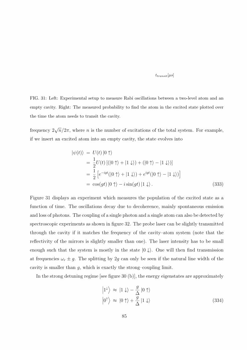
FIG. 31: Left: Experimental setup to measure Rabi oscillations between a two-level atom and an
empty cavity. Right: The measured probability to find the atom in the excited state plotted over
the time the atom needs to transit the cavity.
frequency 2√n/2π, where n is the number of excitations of the total system. For example,
if we insert an excited atom into an empty cavity, the state evolves into
|ψ(t)〉 = U(t) |0 ↑〉
=1
2U(t) [(|0 ↑〉+ |1 ↓〉) + (|0 ↑〉 − |1 ↓〉)]
=1
2
[e−igt(|0 ↑〉+ |1 ↓〉) + eigt(|0 ↑〉 − |1 ↓〉)
]= cos(gt) |0 ↑〉 − i sin(gt) |1 ↓〉 . (333)
Figure 31 displays an experiment which measures the population of the excited state as a
function of time. The oscillations decay due to decoherence, mainly spontaneous emission
and loss of photons. The coupling of a single photon and a single atom can also be detected by
spectroscopic experiments as shown in figure 32. The probe laser can be slightly transmitted
through the cavity if it matches the frequency of the cavity–atom system (note that the
reflectivity of the mirrors is slightly smaller than one). The laser intensity has to be small
enough such that the system is mostly in the state |0 ↓〉. One will then find transmission
at frequencies ωr ± g. The splitting by 2g can only be seen if the natural line width of the
cavity is smaller than g, which is exactly the strong–coupling limit.
In the strong detuning regime [see figure 30 (b)], the energy eigenstates are approximately
∣∣∣1↓⟩ ≈ |1 ↓〉 − g
∆|0 ↑〉∣∣∣0↑⟩ ≈ |0 ↑〉+
g
∆|1 ↓〉 (334)
85
FIG. 32: The top left figure displays an optical experiment to determine the coupling g via spec-
troscopy. A typical result is shown on the top left. The two Lorentzian peaks are separated by 2g
which in this plot is of the same order as the natural line width. Therefore, the strong coupling
limit is not fully achieved. Although recent optics experiments have improved, the most impressive
data from the strong coupling limit comes from circuit cavity QED as shown in the lower figure.
which are almost the product states |1 ↓〉 and |0 ↑〉. The situation is similar for higher levels.
The energy levels are
E|n↓〉 ≈ n(ωr + χ)
E|n↑〉 ≈ n(ωr − χ) + (ωa − χ), (335)
with n = 0, 1, 2, · · · and χ = g2/∆. In effect, the interaction with the atom barely changes
the eigenstates of the system, but depending on the state of the atom, the cavity frequency
gets shifted by ±χ. Although χ is small in the strong coupling regime, in some instances
the frequency of the cavity can be measured to great precision. Therefore, this regime can
be used to readout the state of the atom. This is the most common principle behind the
readout of superconducting qubits.
1. Coupling of photons with Cavity QED
Here we show how a three level atom can be used to couple two photons of different modes
86

a and b. The modes have the same frequency ωr and
opposite polarization. The mode a couples to the atomic
transition |g〉 → |L〉, and the mode b couples to |g〉 →|R〉, as shown to the right. The states |L〉 and |R〉 are
degenerate and have a different magnetic quantum number such that they can be selectively
addressed by photons of different polarization. The Jaynes-Cummings Hamiltonian is
H = ωrN +∆
2
−1 0 0
0 1 0
0 0 1
+ g
a
0 0 0
1 0 0
0 0 0
+ a†
0 1 0
0 0 0
0 0 0
+ b
0 0 0
0 0 0
1 0 0
+ b†
0 0 1
0 0 0
0 0 0
,
(336)
where N is again the total number of excitations. The Hamiltonian can be written in a
block diagonal form
H =
H0 0 0 0 · · ·0 Ha 0 0 · · ·0 0 Hb 0 · · ·0 0 0 Hab · · ·...
......
.... . .
. (337)
H0 = −∆/2 is the Hamiltonian acting on the zero-excitation subspace |0a1bg〉,
Ha, Hb =
−∆/2 g
g ∆/2
. (338)
are acting on the subspaces |1a0bg〉 , |0a0bL〉 and |0a1bg〉 , |0a0bR〉, respectively, and
Hab =
−∆/2 g g
g ∆/2 0
g 0 ∆/2
. (339)
is acting on |1a1bg〉 , |0a1bL〉 , |1a0bR〉. In the dispersive regime ∆ g and for positive
detuning ∆, the ground state within each subspace
|g0〉 ≈ |0a0bg〉 , |ga〉 ≈ |1a0bg〉 , |gb〉 ≈ |0a1bg〉 , |gab〉 ≈ |1a1bg〉 , (340)
have almost no population of the atomic excited states. After a constant energy shift of
∆/2, the corresponding energies are
E0 ≈ 0, Ea = Eb ≈ −g2
∆+
2g4
∆3, Eab ≈ −
2g2
∆+
8g4
∆3. (341)
87
That is, the energy of one photon in each cavity Eab = Ea + Eb + χ3 is by the nonlinearity
factor χ3 = 4g4/∆3 increased compared to the sum of the single photon energies. In other
words, the energy of a photon in mode a depends on the state of mode b. The two qubit
Hamiltonian reads
H =
0 0 0 0
0 ωr + Ea 0 0
0 0 ωr + Ea 0
0 0 0 2(ωr + Ea) + χ3
. (342)
and a C-Phase gate diag1, 1, 1, eiϕ can be achieved by time evolution for t = 2π/(ωr+Ea).
The phase ϕ can be adjusted by the detuning ∆.
XII. ION TRAPS QC
It is fair to say that ion trap QC is the most advanced concept up to date (with the
exception of NMR QC which can not be scaled). Two qubit gates between distant qubits
have been performed with high accuracy. The main difficulty remains the scaling up because
the number of ions in an ion trap is limited.
A. System
The qubit in ion trap QC is a nuclear spin of a single ion. The nuclear spin makes an vary
good qubit because it has decoherence times of up to several hours. Ions are used because
they can be trapped easily. It is not possible to trap an ion by static fields. A typical ion-trap
is shown in Fig. 33. It uses a static field to get an approximately harmonic potential along
the z-axis, and an oscillatory field which on average results in an approximately harmonic
potential in the x and y direction.
The Hamiltonian of the motional degrees of freedom of N trapped ions is
Hm =∑i=1
NM
2
(ω2xx
2i + ω2
yy2i + ω2
zz2i +|~pi|2M2
)+
N∑i,j=1, i<j
e2
4πε0|~ri − ~rj|. (343)
Typically one uses ωx, ωy ωz such that the mutual repulsion of the ions leads to a single
line of ions in the trap. Oscillations of the ions in the x and y directions as well as the
contra directional oscillations in z directions have high frequencies and are not important
88

FIG. 33: A typical ion trap with seven ions (red).
in the following. However, the in-phase oscillations in z direction will be used later and we
therefore introduce the creation and annihilation operators a† and a for this phonon mode.
With laser cooling techniques (Doppler cooling up to the Doppler limit, and then with
sideband cooling) temperatures with
kBT hωz (344)
are achieved, and the ions are let to equilibrate into the motional ground state as well as
the electronic hyperfine ground state.
As a toy model we discuss a two-level spin in a harmonic potential with ωz, but the
generalization to higher dimensional spins and N ions is straight forward. The free particle
Hamiltonian is
H0 = hω0σz + hωza†a. (345)
The interaction Hamiltonian of the spin with a laser field is HI = −~µ · ~B, where ~µ = µ~σ
is proportional to the spin operator and ~B = B~ex cos(kz − ωt + ϕ) is the magnetic field
of the laser. Defining the Rabi-frequency Ω = µB/2h and the Lamb-Dicke parameter
η = 2π√h/2Mωz/λ (the ratio of the motional movement of the ion over the wave length of
the laser), the Hamiltonian is approximately
HI =hΩ
2
(σ+e
i(ϕ−ωt) + σ−e−i(ϕ−ωt)
)+ i
ηhΩ
2
(σ+a+ σ−a
† + σ−a+ σ+a†) (ei(ϕ−ωt) − e−i(ϕ−ωt)
)+ O(η2). (346)
89

The first term is the coupling of a spatially uniform magnetic field. The second term is
due to the spatial variation of the magnetic field around the center of the potential well. It
excites and relaxes the ions state and simultaneously creates and annihilates phonons. Using
the bases |0〉 , |1〉 for the spin and |n〉 for the oscillation, HI couples the eigenstates of
H0 as shown below.
The main transitions at ω0 and the blue and
red sideband transitions. Depending on the
laser frequency one can selectively drive one
of these three transitions.
blaurot
The extension to N spins is done by η → η/√N because all spins move together. If the laser
points to one ion, only this ions electronic state is modified but all ions oscillate together in
phase (→ Mossbauer effect).
B. Quantum computation
An arbitrary single qubit operation is performed by pointing a laser with frequency ω0
to the respective ion. Two-qubit operations are performed in two steps. First the desired
operation is performed between one ion and the two lowest levels of the phonon mode.
Then a SWAP operation between the phonon mode and the other ion is used. Because the
phonons are shared between all ions, it is called a phonon bus qubit. We discuss a C-Phase
gate between the ions with numbers i and j.
90

The C-Phase gate between the ion i and the phonon mode
is done with the help of an auxiliary level |2i〉 of the
ions internal state. Driving a 2π-rotation between |1i1〉and |2i0〉 results in |1i1〉 → − |1i1〉 and |2i0〉 → − |2i0〉.Restricted to the subspace |0i0〉 , |0i1〉 , |1i0〉 |1i1〉this is exactly the C-Phase gate because the levels
|0i0〉 , |0i1〉 , |1i0〉 are not disturbed. A more complicated
scheme is possible without using an auxiliary level.
The SWAP operation is simply achieved by pointing a laser on ion j with the fre-
quency ω0 − ωz to induce a π-rotation between |1j0〉 and |0j1〉:
SWAPj =
1 0 0 0
0 0 1 0
0 −1 0 0
0 0 0 1
. (347)
A CNOT between i and j is then
CNOTij = Hj SWAPj CNOTi SWAP†j Hk, (348)
where the Hadamard gates transform the C-Phaseij into a CNOTij
The first CNOT between two ions was achieved with hyperfine states of Beryllium ions
9Be+. Figure 34 displays the energies of the ion states labeled according to the total spin
~F = ~S + ~I of the nucleon and electron.
The hyperfine states (F,mF) are splitted by means of a static magnetic field of 0.18 mT.
The vibrational modes are denoted by n. The states 2S1/2(2, 2) and 2S1/2(1, 1) are used as
qubit states, and the state 2S1/2(2, 0) as auxiliary level.
Instead of direct driving, so-called Raman transitions via the 2P1/2(2, 2) level are em-
ployed. For that one uses two laser beams with a frequency difference matching the desired
transition of 1.25 GHz. The population of the 2P1/2(2, 2) level can be avoided by a strong
detuning ∆ the lasers from the corresponding transition. That is necessary because this
excited level has a large spontaneous decay rate. The advantage of Raman transitions are
that lasers with optical frequencies can be focused easily on single ions.
To read out the qubit state, one drives the transition 2S1/2(2, 2) → 2P3/2(3, 3). If the
qubit is in the state 2S1/2(2, 2), then the laser will excite the ion. The state 2P3/2(3, 3) then
91

FIG. 34: Some energy levels of 9Be+.
decays by emitting a photon in a random direction. Because of selection rules, the ion can
only relax into 2S1/2(2, 2) and the process starts again. This fluorescence can be measured
with photon detectors. If the qubit is in the state 2S1/2(1, 1), then the laser light does not
match any possible transition frequency and no photons are observed.
C. Limitations
The decoherence times of the motional states is much shorter compared to the hyperfine
states. Much improvement is possible by exciting them only for a short time.
More than 20 ions per trap are difficult, the limitation is due to non-center-of-mass
phonons. For large scale QC it is necessary to couple many ion traps.
XIII. LIQUID STATE NMR QC
The qubit is represented by hyperfine states like in ion trap QC. The main idea of nuclear
magnetic resonance QC is to circumvent the shared phonons (weak induced coupling and
strong decoherence) by using several nuclear spins of a single molecule as qubits. The spins
92

are then sufficiently close together to interact via dipole interaction and electron induced in-
teraction. The downside is that the many vibrational degrees of freedom makes it difficult to
trap and cool the molecules. Therefore, they are dissolved in a solvent at room temperature.
Because all spins used for qubits have different transition frequencies (to the contrary
to ion trap QC), one can selectively address a single qubit without focusing the electro
magnetic wave to the respective atom. The manipulation and measurement of nuclear spins
with radio waves is very well developed (→ chemistry), which is a big advantage.
There are two downsides of NMR QC which can be overcome by interesting new concepts.
First, the magnetic moment of a single nuclear spin is too small to be detectable. Therefore
one uses about 108 molecules to enhance the signal. Therefore, we are considering an
ensemble of quantum computers! Second, the liquid samples can not be cooled well and
kBT hω0 results in an almost random direction of the spins. The initialization into a
pure state is far from possible. The solution to that problem will be discussed later.
There is a further conceptional limitation concerning the scaling. The number of atoms
with sufficiently distinct transition frequencies is limited. It is clear that large scale liquid
state NMR QC is not possible with the methods outlined in this section. Nevertheless,
it was possible to perform some small scale quantum computing which served as proof of
principle and major milestone in the history of QC. Furthermore, many control techniques
were developed and optimized in NMR systems, and later used in other architectures.
A. System
Molecule:
• N protons (or other spin-1/2 nucleons like 13C, 15N, 19F, 31P) with ω0 ≈ 500 MHz in
a magnetic field of 10 T.
• Different protons have slightly different ω0 due to different neighboring atoms shielding
the magnetic field: ∆ω0 ≈ 10− 100 kHz.
• No inter molecular interaction due to low density of molecules → Ensemble of inde-
pendent quantum computers.
The setup is shown in Fig. 35. The static field B0 has to be homogeneous up to a
relative error of 10−9 within a volume of 1 cm3. The radio frequency coil is not only used
93

FIG. 35: A typical setup for liquid state NMR.
to manipulate the nuclear spins, but also for their readout. That is because the precessing
nuclear spins generate an RF-field, inducing a current in the coil which can be detected.
B. Time evolution
The Hamiltonian of a single nuclear spin j is
Hj =hω0j
2σzj + gjh(σxj cosωjt+ σyj sinωjt)
rot. frame=
h
∆j/2 gj
gj −∆j/2
, (349)
with ∆j = ω0j − ωj. The dipole coupling between two spins i and j is
HDij =
µ1µ2h
4|rij|3[~σi · ~σj − 3(~σi · ~n)(~σj · ~n)] , (350)
where ~n = ~rij/|rij| and ~rij is the vector from spin i to spin j. Because the molecules in a
liquid are rotating fastly, the system experiences the Hamiltonian averaged over all directions
of ~n, which vanishes for HDij :
〈HDij 〉~n = 0. (351)
Therefore, one only has to consider the electron mediated coupling
HJij =
hJ
4~σi · ~σj
=hJ
4~σz,i · ~σz,j +
hJ
8(~σ+,i · ~σ−,j + ~σ,−i · ~σ+,j)
94

≈ hJ
4~σz,i · ~σz,j, (352)
where the RWA was used which is valid if the precession frequencies of the to spins are
sufficiently different ω0,i − ω0,j J .
All single qubit operations can be performed with the Hamiltonian Eq. (349). They have
to be performed sufficiently fast, such that the relatively weak two qubit coupling (which
can not be switched off) can be neglected. For two qubit operations we write the non-driven
two qubit Hamiltonian as
Hsys = aσz1 + bσz2 + cσz1 ⊗ σz2 (353)
Therefore, the free evolution for T = π/4c results in a C-phase gate up to one qubit rotations
around the z-axis. The latter can be undone by further single qubit rotations. With these
thechniques (and spin echo) high precision gates are possible.
Decoherence:
• Inhomogeneity of B0: Can be mostly corrected by spin echo techniques.
• Dipole spin-spin coupling: Can not be corrected, but is minimized with large(!) tem-
perature because the molecules rotate faster and the interaction averaged to zero.
• T1 and T2 can be easily measured. E.g. for T1 a π-pulse is applied to excite the system.
After waiting some time for the system to relax, a π/2-pulse leads to a superposition
state and its precession strength give the coherence.
• T1 and T2 are used in NMR-imaging to distinguish between different molecules.
C. Magnetization Readout
The output of an experiment is the free induction decay signal
V (t) = V0
[e−iHt/hρeiHt/h
∑k
(iσxk + σyk
](354)
The signal oscillates with the eigen frequencies of the system and usually the Fourier trans-
form V (ω) is measured.
Figure 36 shows the spectrum of 13C labeled trichloroethylene near the typical transition
frequency of 13C. Because of the different shielding of the magnetic field the frequency of
95

C C
Cl
ClCl
H
FIG. 36: The carbon spectrum of 13C labeled trichloroethylene. The proton and two carbons give
a three qubit system
the left Carbon is about 600 MHz lower. Furthermore, because the left 13C couples to the
right 13C and the proton, four lines can be seen; depending on their state, the left 13C has
a modified transition frequency. The proton splits the lines by 200 MHz, the right 13C by
about 100 MHz. The right 13C transition frequency is also split into four peaks, but the
splitting due to the proton is tine because the proton is far away from the right 13C.
D. Initial state and “labeling”
For the initial state the system is let to equilibrate in the static field B0, which may take
a few minutes. The state of the system of all nuclear spins is then
ρ =e−H/kBT
tr(e−H/kBT)
≈ 2−N(1−H/kBT ), (355)
where typically H/kBT ≈ 10−4! For small couplings this state is diagonal in the Z-basis
|0, . . . , 0, 0〉 , |0, . . . , 0, 1〉 , . . . , |1, . . . , 1, 1〉.Now we tackle the problem how to use an almost random state for quantum computing.
For simplicity we assume computation with two qubits only. Instead of the desired initial
96

ground state we have
ρ1 =
a 0 0 0
0 b 0 0
0 0 c 0
0 0 0 d
6=
1 0 0 0
0 0 0 0
0 0 0 0
0 0 0 0
(356)
With the help of CNOT one can construct the unitary operator P with
ρ2 = Pρ1P† =
a 0 0 0
0 c 0 0
0 0 d 0
0 0 0 b
, ρ3 = P †ρ1P =
a 0 0 0
0 d 0 0
0 0 b 0
0 0 0 c
(357)
Any computation U is now performed with each ρ(t = 0) = ρ1, ρ2, ρ3 at separate times and
the results are averaged to give
∑k
UρkU† = (4a− 1)U
1 0 0 0
0 0 0 0
0 0 0 0
0 0 0 0
U † + (1− a)
1 0 0 0
0 1 0 0
0 0 1 0
0 0 0 1
(358)
Because any measurement of spin operators are traceless, the last term does not give a
measurement signal. The sum of all measurements give the same result as if the
initial system where in a pure state, but with a signal reduced by the factor
(4a− 1)! This technique is called temporal labeling.
Other similar techniques are spatial labeling, where the three computations are performed
simultaneously but at either different systems or at different parts of one system. In log-
ical labeling one performs only one experiment, but uses three mixed state qubits for a
computation involving two pure states.
The problem with labeling is that α is only slightly more than 1/4 if the thermal state
is close to a random state. Even worst, this small signal reduces exponentially with the
number of qubits because the probability of being in the ground state
p00...0 =1
Z〈0|⊗N e−H/kBT |0〉⊗N ∝ N2−N (359)
reduces exponentially. Therefore, liquid NMR QC can not be used for large scale QC.
97

Nevertheless, NMR QC is the most advanced technique and it has been used to perform
impressive proof of principle experiments, such as the factorization of 15 = 3 × 5, or the
implementation of Grovers search algorithm. Also, in trichloroethylene, the protons state
got teleported the the right carbon.
XIV. ELEMENTS OF QUANTUM ERROR CORRECTION
Quantum error correction is a very large field by itself. We only discuss the correction of
errors during information transfer and say a few words about gate errors at the end of this
section. The basic idea is to encode one logical bit into several physical bits. This way, if
one physical bit gets corrupted, there is still sufficient information to recover the logical bit.
A. Classical error correction
Some components of classical hardware, such as modems and CD–players, require error
correction. Lets assume Alice wants to transfer information to Bob, but each transferred
bit can undergo bit flip error with probability p. The simplest code is the repetition code.
Before sending the information to Bob, Alice copies each bit twice
0→ 000
1→ 111. (360)
This process is called encoding. If Alice sends a 000, Bob may obtain one of the following
states:
000transmission−−−−−−−−−→
000 with probability (1− p)3
001 with probability (1− p)2p
010 with probability (1− p)2p
100 with probability (1− p)2p
011 with probability (1− p)p2
101 with probability (1− p)p2
110 with probability (1− p)p2
111 with probability p3
. (361)
98

Bob decodes the message using majority voting, that is
000, 001, 010, 100 → 0
111, 110, 101, 011 → 1. (362)
To perform the decoding, of course he has to be able to measure every physical bit sent to
him. According to Eq. (361), the repetition code reduces the error rate from p to 3p2− 2p3.
Of course one can arbitrarily reduce the error rate if enough recourses are available.
If bob wants to send the information further, he doesn’t need to decode and encode again,
he may just correct for the error by
000, 001, 010, 100 → 000
111, 110, 101, 011 → 111. (363)
B. Quantum error correction
Apparent difficulties with quantum error correction include:
• No cloning theorem forbids copying the qubits: |ψ〉 → |ψ〉 |ψ〉 |ψ〉 is not possible.
• Measurement destroys the state: |ψ〉 |ψ〉 |ϕ〉 → |ψ〉 |ψ〉 |ψ〉 is not possible.
• Two types of errors: Bit flip and phase flip.
• Errors are continuous.
Quite amazingly, quantum error correction is still possible. We first outline the bit-flip
code which corrects for bit-flips which happen with probability p. We encode
|0〉 → |0L〉 = |000〉
|1〉 → |1L〉 = |111〉 (364)
It is important to realize that this is no copying of a quantum state, because
a |0〉+ b |1〉 → a |000〉+ b |111〉 6= (a |0〉+ b |1〉)⊗3, (365)
99

where we introduced the notation |ψ〉⊗n = |ψ〉⊗|ψ〉⊗ · · · ⊗ |ψ〉. The encoding can be done with
simple CNOT-gates as shown to the right.
For the error diagnoses, one could just measure the state of the three physical Qubits.
Obtaining e.g. |010〉 then indicates that the second qubit flipped. However, the measurement
destroyed the superpositions of |0〉 and |1〉 and it is not possible to recover the desired state
|ψL〉 = a |000〉+ b |111〉.The key idea is to only measure if the qubits are in the same state or not, and if not,
then which qubit differs from the other two. This can be done without measuring the actual
state of each qubit by measuring the four error syndromes :
P0 = |000〉〈000|+ |111〉〈111|
P1 = |100〉〈100|+ |011〉〈011|
P2 = |010〉〈010|+ |101〉〈101|
P3 = |001〉〈001|+ |110〉〈110| (366)
These are all Hermitian operators and can easily be measured (If one is restricted to one
qubit measurements, then one needs to transform the three qubit state appropriately before
the measurement. Using the same transformation as for the encoding results in P0 →1l ⊗ |00〉〈00| , P1 → 1l ⊗ |11〉〈11| , P2 → 1l ⊗ |10〉〈10|, and P3 → 1l ⊗ |01〉〈01|). If the
measurement of P0 gives the result one, then we know that all three qubits are in the same
state and assume that no qubit flipped. If P1 results in one, then the state of the first qubit
differs from the state of the other qubits. We then conclude that the first qubit must have
flipped, and correct this error by flipping it again. Similar for the other syndromes. As an
example we look at the state after each step for a bit-flip error on qubit two. Note that the
projective measurement does not alter the state
a |000〉+ b |111〉 bit-flip−−−−→error
a |010〉+ b |101〉 projection−−−−−−−→with P2
a |010〉+ b |101〉 correction−−−−−−−→with σ(2)
x
a |000〉+ b |111〉
Like in the classical scheme, we can only correct the error if maximally one qubit flipped.
The error rate is again reduced from p to 3p2 − 2p3.
100

Next we discuss the phase-flip code. Noting that a phase flip
|0〉 → |0〉
|1〉 → − |1〉 (367)
is equivalent to a bit-flip in the basis |±〉, we only have to change the basis and we
can use the bit-flip code to correct for phase-flip errors. The encoding is according to
|0〉 → |0L〉 = |+ + +〉
|1〉 → |1L〉 = |− − −〉
H
H
H
and the four error syndromes are Pj = H⊗3PjH⊗3.
The Shore code combines the bit-flip and phase-flip codes to correct for both errors:
|0L〉=(|000〉+|111〉)⊗ (|000〉+|111〉)⊗ (|000〉+|111〉)√
8
|1L〉=(|000〉−|111〉)⊗ (|000〉−|111〉)⊗ (|000〉−|111〉)√
8
H
H
H
Quite amazingly, the Shore code does not only correct phase-flips and bit-flips, but any
error, unitary or not unitary (such as decoherence). We only outline the proof. Every error
is a quantum map (completely positive and trace preserving) and can be written in Kraus
representation
|ψ〉〈ψ| →∑j
Kj |ψ〉〈ψ|K†j . (368)
The Kraus operators can in turn be decomposed as
Kj = kj0 1l + kj1σx + kj2σz + kj3σxσz, (369)
that is, Kj |ψ〉 is a superposition of the states without error, with a bit-flip error, with a
phase-flip error and with both errors. Measuring an error syndromes then collapses the
101

state to be either without error, or with one of the errors, depending on the measurement
outcome (but does not collapse a |0L〉+b |1L〉). This error is then corrected by the usual error
correction. As an example consider an
1 0
0 eiφ
-error on the first qubit. The measurement
of P1 gives the result one with probability sin2(φ/2) and in this case the state is projected
onto σ(1)z |ψL〉 as if it had undergone a full phase-flip. The error correction protocol then
corrects this error by another σ(1)z . With probability cos2(φ/2), the measurement of P0 gives
the result one. The state is then projected onto the desired state a |0L〉+b |1L〉 and the error
correction protocol leaves it like that. It is remarkable that a continuous set of errors can
be corrected by a finite number of mechanisms.
The Shore code reduces the error rate from p to 36p2 + O(p3). If the error rate p < pc
is smaller than a critical error rate of pc ≈ 1/36, then the error can be reduced further by
concatenation. E.g. encoding a logical qubit into 81 physical qubits according to
|0LL〉=(|0L0L0L〉+|1L1L1L〉)⊗ (|0L0L0L〉+|1L1L1L〉)⊗ (|0L0L0L〉+|1L1L1L〉)√
8
|1LL〉=(|0L0L0L〉−|1L1L1L〉)⊗ (|0L0L0L〉−|1L1L1L〉)⊗ (|0L0L0L〉−|1L1L1L〉)√
8
results in an error rate of 36(36p2)2 + O(p6). This process can be continued to achieve an
arbitrarily small error rate as long as the error rate for a physical qubit is below the critical
pc.
The threshold theorem is essential to the success of quantum computing. It states that
as long as the error rate is below a critical threshold rate and if sufficient resources are
available, then arbitrarily complex quantum computing is possible due to concatenation of
error correcting codes. The actual threshold is hard to state because one also has to take into
account errors in the encoding process and in the syndrome measurements. Furthermore,
for a simple single qubit transformation on the logical qubit one needs to perform a nine
qubit transformation if one uses the Shore code. Typical values for the threshold found in
the literature range between 10−2 and 10−4.
102

XV. TOPOLOGICAL IDEAS
A. Error correction: stabilizers formalism
The error correction codes can be formulated using ”code stabilizers” (D. Gottesmann).
To motivate, consider once again the simplest 3-bit code:
∣∣∣0⟩ = |000〉 and∣∣∣1⟩ = |111〉 . (370)
Consider operators S1 = Z1Z2 (we introduce a notation Zi ≡ σzi) and S2 = Z2Z3. We have
S1
∣∣∣0⟩ =∣∣∣0⟩
S1
∣∣∣1⟩ =∣∣∣1⟩
S2
∣∣∣0⟩ =∣∣∣0⟩
S2
∣∣∣1⟩ =∣∣∣1⟩ . (371)
One says that S1 and S2 stabilize the code. Measuring S1 or S2 we will not distinguish
between the two logical states. Yet measuring S1 and S2 we can detect any one-bit Xi error
(spin flip). That is if initially we have
|ψ〉 = α∣∣∣0⟩+ β
∣∣∣1⟩ (372)
and, then an error happens, i.e., our state is now, e.g., X1 |ψ〉 = α |100〉+β |011〉. Measuring
both S1 and S2 we obtain S1X1 |ψ〉 = −X1 |ψ〉 and Z2X1 |ψ〉 = X1 |ψ〉 The state X1 |ψ〉 is an
eigenstate of both S1 and S2 and it remains intact after the measurement. The combination
S1 = −1, S2 = 1 uniquely distinguishes the X1 error from X2 and X3. Thus we can now
correct, e.g, by applying X1 once again.
Instead of specifying the code states it is sufficient to specify the stabilizers. The code
subspace is uniquely determined by the conditions S1 |ψ〉 = |ψ〉 and S2 |ψ〉 = |ψ〉.A detectable error operator anti commutes necessarily with at least one of the stabilizers.
In our case E = X1 and X1, S1 = 0 whereas [X1, S2] = 0. The anti commuting gives rise
to the negative eigenvalues. Indeed if an error operator E anti commutes with the stabilizer
S we obtain
SE |ψ〉 = −ES |ψ〉 = −E |ψ〉 . (373)
103

1. Stabilizers of the Shor code
The 9-bit code of Shor is given by
∣∣∣0⟩ =1
23(|000〉+ |111〉)(|000〉+ |111〉)(|000〉+ |111〉)∣∣∣1⟩ =
1
23(|000〉 − |111〉)(|000〉 − |111〉)(|000〉 − |111〉) . (374)
The 8 stabilizers of this code read
S1 = Z1Z2
S2 = Z2Z3
S3 = Z4Z5
S4 = Z5Z6
S5 = Z7Z8
S6 = Z8Z9
S7 = X1X2X3X4X5X6
S8 = X4X5X6X7X8X9 . (375)
Detectable errors, e.g., X1 . . . X9, Z1 . . . Z9, Y1 . . . Y9 etc. For example X1 can be distin-
guished from Y1 because X1 anti commutes with S1 only, while Y1 anti commutes with S1
and S7.
Z1 seems to be indistinguishable from Z2. Indeed both anti commute with S7 only. Thus
by measuring all 8 stabilizes and getting −1 only for S7 we can only conclude that one of
the three possible errors, i.e. Z1, Z2, Z3 happened. These three are all corrected by, e.g.,
applying Z1.
B. Toric code
This code has been proposed by Kitaev.
104

C. Majorana bound states
We consider another model proposed by Kitaev, a 1-D p-wave superconductor. The
Hamiltonian reads
H =N−1∑j=1
[−tc†jcj+1 + ∆cjcj+1 + h.c.
]. (376)
We assume the order parameter ∆ to be real. We introduce the Majorana operators (not
really related to Majorana particles)
cj =1
2(γA,j + iγB,j)
c†j =1
2(γA,j − iγB,j) . (377)
The inverse relations read
γA,j = cj + c†j
γB,j = −i(cj − c†j) . (378)
The commutation relations of the Majorana operators read γα,j, γα′,j′+ = 2δα,α′δj,j′ . Here
α, α′ = A/B. In particular γ2α,j = 1. Also these operators are Hermitian, γ†α,j = γα,j.
Substituting we obtain
H =1
4
N−1∑j=1
[−t(γA,j − iγB,j)(γA,j+1 + iγB,j+1) + ∆(γA,j + iγB,j)(γA,j+1 + iγB,j+1) + h.c.] .
(379)
The AA and BB terms vanish and we are left with
H =i
2
N−1∑j=1
[(−t+ ∆)γA,jγB,j+1 + (t+ ∆)γB,jγA,j+1] . (380)
An interesting situation arises if ∆ = t. We obtain
H = iN−1∑j=1
tγB,jγA,j+1 . (381)
Two Majoranas are not involved in this Hamiltonian and, thus, commute with it. These are
γL ≡ γA.1 and γR ≡ γB,N . This means that all the eigenstates including the ground state
are double degenerate. Indeed from γL and γR we can form a new pair of Fermi operators
d ≡ 1
2(γL + iγR) and d† ≡ 1
2(γL − iγR) . (382)
105

The operators d and d† commute with the Hamiltonian. The doubling of the states in
according to the occupation number d†d. If there exist a ground state |g0〉 such that d |g0〉 =
0, then also the state |g1〉 = d† |g0〉 is a ground state, i.e., it has the same energy.
What happens if ∆ 6= t (but they are still close). We start again from (376) and rewrite
it as
H =N−1∑j=1
[tc†jcj+1 + ∆cjcj+1 + h.c.
]. (383)
[1] M. V. Berry, Proc. R. Soc. Lond. A 414, 31 (1987).
[2] G. Lindblad, Commun. Math. Phys. 48, 119 (1976).
[3] G. S. V. Gorini, A. Kossakowski, J. Math. Phys. 17, 821 (1976).
[4] J. von Neumann, Mathematische Grundlagen der Quantenmechanik (Springer-Verlag, 1968).
[5] B. D. Josephson, Physics Letters 1, 251 (1962).
[6] V. Ambegaokar and A. Baratoff, Phys. Rev. Lett. 10, 486 (1963).
[7] V. Ambegaokar and A. Baratoff, Phys. Rev. Lett. 11, 104 (1963).
[8] A. O. Caldeira and A. J. Leggett, Phys. Rev. Lett. 46, 211 (1981).
[9] A. O. Caldeira and A. J. Leggett, Annals of Physics 149, 374 (1983).
[10] H. Mabuchi and A. C. Doherty, Science 298, 1372 (2002).
[11] If the system is initially entangled with the environment, then VS is generally not positive.
106