physics of f-theory compactifications without section · physics of f-theory compacti cations ......

Physics of F-theory compactificationswithout section

Inaki Garcıa-Etxebarria

29th July, 2014

in collaboration with L. Anderson, T. Grimm and J. Keitel

arXiv:1406.5180

F-theory without section

Most F-theory model building is done for spaces with a section.

In this talk I would like to discuss what happens whenever thetorus fibration does not have a section. I will do this for Calabi-Yauthreefolds.

What is the 5d theory of M-theory on such spaces?

Does a F-theory limit exist?

How does the 6d theory look like?

Other interesting questions that I will not discuss: relation to[Morrison Braun, Morrison Taylor], statements in other dimensions,pheno applications, . . . .

More on the computation of the effective action has been described inGrimm’s talk, here I will focus on the geometry.

Fibrations with and without section

We study Calabi-Yau threefolds X that are T 2 fibrations:

π : X → B (1)

with B a complex surface, and π−1(p) topologically a T 2 forgeneric p ∈ S.

The examples that we construct have a modulus controlling thesize of the fiber, so taking the F-theory limit

vol(T 2)→ 0 (2)

makes sense.

We study Calabi-Yau threefolds X that are T 2 fibrations:

π : X → B (1)

with B a complex surface, and π−1(p) topologically a T 2 forgeneric p ∈ S.

The examples that we construct have a modulus controlling thesize of the fiber, so taking the F-theory limit

vol(T 2)→ 0 (2)

makes sense.

A section σ is defined by a continuous map σ : B → X of the baseB into the total space X such that

π(σ(p)) = p (3)

for all p ∈ B.

In other words, a globally defined choice of point foreach fiber. Algebraically, we will want a divisor σ such that σ ∼ Band σ · F = 1, with F the curve representing the fiber of thefibration.

π(σ(p)) = p (3)

for all p ∈ B. In other words, a globally defined choice of point foreach fiber.

Algebraically, we will want a divisor σ such that σ ∼ Band σ · F = 1, with F the curve representing the fiber of thefibration.

π(σ(p)) = p (3)

for all p ∈ B. In other words, a globally defined choice of point foreach fiber. Algebraically, we will want a divisor σ such that σ ∼ Band σ · F = 1, with F the curve representing the fiber of thefibration.

For physics purposes a slight generalization is very important: weallow for rational sections: they are generically sections, but atcertain loci of the base, where the fiber becomes singular, theymay wrap full components of the (resolved) fiber.

We’ll encounter examples later. These rational sections aresomewhat subtle to treat, but they are well understood by now.

For physics purposes a slight generalization is very important: weallow for rational sections: they are generically sections, but atcertain loci of the base, where the fiber becomes singular, theymay wrap full components of the (resolved) fiber.

We’ll encounter examples later. These rational sections aresomewhat subtle to treat, but they are well understood by now.

A section need not exist.

A simple and well known class of examples are principal bundles,which have a section iff they are trivial.

A simple example is the boundaryof the Mobius strip, viewed as aπ : S1 → S1 fibration. The fiberis Z2 (two points), and it lacks asection.

Another well known example isS3, with fibration mapπ : S3 → S2 and generic fiber S1.

For the T 2 fibrations appearing in string theory there is no suchgeneral results, and it depends on the case.

One section

This is the familiar case. Any fibration with at least one section isbirational (i.e., connected by blow-ups) to a possibly singularWeierstrass model. [Nakayama]

y2 = x3 + fxz4 + gz6 (4)

with f, g appropriate sections of line bundles on the base B, and (x, y, z)coordinates on P2,3,1. More generically, this is a particular representationof T 2 as a degree 6 polynomial in P2,3,1. A section is given simply bytaking z = 0, independent of the particular form of f and g.

One section

y2 = x3 + fxz4 + gz6 (4)

with f, g appropriate sections of line bundles on the base B, and (x, y, z)coordinates on P2,3,1. More generically, this is a particular representationof T 2 as a degree 6 polynomial in P2,3,1.

A section is given simply bytaking z = 0, independent of the particular form of f and g.

One section

y2 = x3 + fxz4 + gz6 (4)

with f, g appropriate sections of line bundles on the base B, and (x, y, z)coordinates on P2,3,1. More generically, this is a particular representationof T 2 as a degree 6 polynomial in P2,3,1. A section is given simply bytaking z = 0, independent of the particular form of f and g.

Many sections

For every free factor of the group of sections (the Mordell-Weilgroup) one gets an extra U(1). Torsion factors give interesting infoabout the global structure of gauge groups. [Talk by Mayrhofer.]

Many sections

The previous result still applies: every such fibration is birational toa Weierstrass model. Nevertheless, for studying fibrations withmany sections this is not always the most convenientrepresentation. For example, for fibrations with two sections, abetter suited representation is as a Calabi-Yau equation onBl(0,1,0) P1,1,2 [Morrison Park]. More on this soon.

No section

In general we cannot find a section, at best we can find ann-section: an holomorphic divisor projecting to the full base, butintersecting the fiber n times, n > 1. (In our examples, n = 2, buta similar story clearly holds for n > 2 too.)

Not having a section is fairly generic, in Jan Keitel’s talk we learnedthat fibrations without (toric) section furnish approximately 10% ofthe fibers realized as nef partitions of threefold toric varieties.

No section

In general we cannot find a section, at best we can find ann-section: an holomorphic divisor projecting to the full base, butintersecting the fiber n times, n > 1. (In our examples, n = 2, buta similar story clearly holds for n > 2 too.)

Not having a section is fairly generic, in Jan Keitel’s talk we learnedthat fibrations without (toric) section furnish approximately 10% ofthe fibers realized as nef partitions of threefold toric varieties.

Understanding fibrations without section

The subtle features of F-theory on such a manifold, which definesa 6d field theory, are best understood upon compactification on acircle, giving a 5d theory T5. This should be equivalent to studyingM-theory on X in a particular limit. We obtain information on the6d theory by imposing

T5 = M/X

In order to compare the 5d effective field theories we have toconsistently integrate out the massive matter in the 6d→5dreduction. From the M-theory sugra reduction perspective thismassive matter simply does not appear.

But massive fermions in 5d can induce anomalies under largegauge transformations. If we integrate them out the anomaly mustremain (as a contribution to a Chern-Simons term). In other words,there are one-loop corrections to the classical Chern-Simons terms.

T5 = M/X

In order to compare the 5d effective field theories we have toconsistently integrate out the massive matter in the 6d→5dreduction.

From the M-theory sugra reduction perspective thismassive matter simply does not appear.

T5 = M/X

The Chern-Simons terms in the 5d theory have the form

SCS = − 1

∫M4,1

kIJKAI ∧ F J ∧ FK − 1

∫M4,1

kIAI ∧ tr(R∧R)

and shift according to

kΛΣΘ 7→ kΛΣΘ + cAFF qΛqΣqΘ sign(m) (6)

kΛ 7→ kΛ + cARR qΛ sign(m) , (7)

for each massive field we integrate out, with

spin-1/2 fermion self-dual tensor Bµν spin-3/2 fermion ψµcAFF

12 −2 5

2cARR −1 −8 19

So one-loop Chern-Simons terms, which are topological in nature(since they encode anomalies) are rather robust. Matching theM-theory sugra reduction with the action after integrating out thefermions turns out to be very constraining, and allows us todetermine the spectrum.

(I’ll omit any more detailed discussion ofthis point, since Thomas discussed it already.)

The M-theory M/X is determined in the examples we consider bya conifold transition from a compactification on spaces with twosections.

So one-loop Chern-Simons terms, which are topological in nature(since they encode anomalies) are rather robust. Matching theM-theory sugra reduction with the action after integrating out thefermions turns out to be very constraining, and allows us todetermine the spectrum. (I’ll omit any more detailed discussion ofthis point, since Thomas discussed it already.)

Conifold transitions in M-theory

small resolutiondeformation

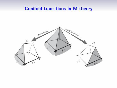
The singular conifold is given by

z21 + z2

2 + z23 + z2

in C4. Singularity at (0, 0, 0, 0) (f = df = 0).

Deformation

Change the defining equation to

z21 + z2

2 + z23 + z2

4 = ε . (8)

f = df = 0 has no solution anymore, so the space is smooth.There is a finite size S3 where the singularity was.

z21 + z2

2 + z23 + z2

Deformation

Change the defining equation to

z21 + z2

2 + z23 + z2

4 = ε . (8)

f = df = 0 has no solution anymore, so the space is smooth.There is a finite size S3 where the singularity was.

z21 + z2

2 + z23 + z2

Small resolution

Replace the singularity by a “small resolution”, which is a newspace with a map to the original singular space which is anisomorphism away from the singular point. Rewrite the conifoldequation as xy − zw = 0. Then the resolved space is(

x zw y

)= 0 (9)

where (a, b) ∈ P1. One finds a full P1 where the singularity was.

Low energy physics of M-theory on a conifoldLocal description

Fairly mild singularity: it can be completely described by effectivefield theory in 5 dimensions [Strominger]:

At the singular point there is a 5d N = 1 theory with gauge group U(1)(from reducing C3 on the two-sphere) and a charged hypermultiplet(from an M2 on the contracting two-sphere).

Deformation corresponds to a Higgsing: i.e. giving a vev to thehypermultiplet, so the U(1) vector multiplet becomes massive.

Resolution corresponds to going into a Coulomb branch: giving a vev tothe scalar in the U(1) vector multiplet, so the hyper becomes massive.

Low energy physics of M-theory on a conifoldLocal description

Fairly mild singularity: it can be completely described by effectivefield theory in 5 dimensions [Strominger]:

At the singular point there is a 5d N = 1 theory with gauge group U(1)(from reducing C3 on the two-sphere) and a charged hypermultiplet(from an M2 on the contracting two-sphere).

Deformation corresponds to a Higgsing: i.e. giving a vev to thehypermultiplet, so the U(1) vector multiplet becomes massive.

Resolution corresponds to going into a Coulomb branch: giving a vev tothe scalar in the U(1) vector multiplet, so the hyper becomes massive.

Conifold transitions for global models

The global picture is similar, but there can be relations betweenthe local cycles, which require some more careful counting[Greene Morrison Strominger, Mohaupt Saueressig].

Consider the case in which P conifold points are transitioningsimultaneously. These curves are typically related by R relations inhomology, so this implies that P −R curve classes are transitioningsimultaneously.

Studying the low energy theory, one sees that there are R flat directionsin which one can Higgs the hypers. Along these directions the P −RU(1) vector multiplets get a mass, by pairing up with the P −R non-flatdirections.

The global picture is similar, but there can be relations betweenthe local cycles, which require some more careful counting[Greene Morrison Strominger, Mohaupt Saueressig].

Consider the case in which P conifold points are transitioningsimultaneously. These curves are typically related by R relations inhomology, so this implies that P −R curve classes are transitioningsimultaneously.

Studying the low energy theory, one sees that there are R flat directionsin which one can Higgs the hypers. Along these directions the P −RU(1) vector multiplets get a mass, by pairing up with the P −R non-flatdirections.

Starting from the resolved side

(nH , nV ) = (h2,1(X) + 1, h1,1(X)− 1) . (10)

P massless hypers appear when we reach the conifold point

(nH , nV )→ (h2,1(X) + 1 + P, h1,1(X)− 1) (11)

and then, giving a vev to the R flat directions

(nH , nV )→ (h2,1(X) + 1 +R, h1,1(X)− 1− P +R) . (12)

From here we can read the Hodge numbers of the deformed side

(h2,1(X ), h1,1(X )) = (h2,1(X) +R, h1,1(X)− P +R) . (13)

(nH , nV ) = (h2,1(X) + 1, h1,1(X)− 1) . (10)

(nH , nV )→ (h2,1(X) + 1 + P, h1,1(X)− 1) (11)

(nH , nV )→ (h2,1(X) + 1 +R, h1,1(X)− 1− P +R) . (12)

(h2,1(X ), h1,1(X )) = (h2,1(X) +R, h1,1(X)− P +R) . (13)

(nH , nV ) = (h2,1(X) + 1, h1,1(X)− 1) . (10)

(nH , nV )→ (h2,1(X) + 1 + P, h1,1(X)− 1) (11)

(nH , nV )→ (h2,1(X) + 1 +R, h1,1(X)− 1− P +R) . (12)

(h2,1(X ), h1,1(X )) = (h2,1(X) +R, h1,1(X)− P +R) . (13)

(nH , nV ) = (h2,1(X) + 1, h1,1(X)− 1) . (10)

(nH , nV )→ (h2,1(X) + 1 + P, h1,1(X)− 1) (11)

(nH , nV )→ (h2,1(X) + 1 +R, h1,1(X)− 1− P +R) . (12)

(h2,1(X ), h1,1(X )) = (h2,1(X) +R, h1,1(X)− P +R) . (13)

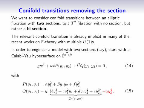
Conifold transitions removing the sectionWe want to consider conifold transitions between an ellipticfibration with two sections, to a T 2 fibration with no section, butrather a bi-section.

The relevant conifold transition is already implicit in many of therecent works on F-theory with multiple U(1)s.

In order to engineer a model with two sections (say), start with a

Calabi-Yau hypersurface on P1,1,2

gw2 + wtP (y1, y2) + t2Q(y1, y2) = 0 , (14)

P (y1, y2) = αy21 + βy1y2 + fy2

Q(y1, y2) = y1 (by31 + cy2

1y2 + dy1y22 + ey3

2)︸︷︷︸Q′(y1,y2)

+ay42 . (15)

Conifold transitions removing the sectionWe want to consider conifold transitions between an ellipticfibration with two sections, to a T 2 fibration with no section, butrather a bi-section.

The relevant conifold transition is already implicit in many of therecent works on F-theory with multiple U(1)s.

In order to engineer a model with two sections (say), start with a

Calabi-Yau hypersurface on P1,1,2

gw2 + wtP (y1, y2) + t2Q(y1, y2) = 0 , (14)

P (y1, y2) = αy21 + βy1y2 + fy2

Q(y1, y2) = y1 (by31 + cy2

1y2 + dy1y22 + ey3

2)︸︷︷︸Q′(y1,y2)

+ay42 . (15)

Conifold transitions removing the section

This space will have two sections whenever a = 0.

Set y1 = 0. The Calabi-Yau equation reduces to

w(gw + tf) = 0 (16)

So our global choice of point in the fiber is given by y1 = w = 0(one section), and y1 = 0, (w, t) = (−f, g) (another section).

Each section is associated to a divisor, and together they give riseto U(1)× U(1) vector bosons in 5d by reduction of C3 on thePoincare dual two-forms.

This space will have two sections whenever a = 0.

Set y1 = 0. The Calabi-Yau equation reduces to

w(gw + tf) = 0 (16)

So our global choice of point in the fiber is given by y1 = w = 0(one section), and y1 = 0, (w, t) = (−f, g) (another section).

Each section is associated to a divisor, and together they give riseto U(1)× U(1) vector bosons in 5d by reduction of C3 on thePoincare dual two-forms.

This space is singular. It has conifold singularities aty1 = w = e = f = 0. (Easy to check that these are solutions ofφ = dφ = 0, with φ = 0 the Calabi-Yau equation defining thefibration.)

We know what to do: resolve or deform!

This space is singular. It has conifold singularities aty1 = w = e = f = 0. (Easy to check that these are solutions ofφ = dφ = 0, with φ = 0 the Calabi-Yau equation defining thefibration.)

We know what to do: resolve or deform!

Conifold transitions removing the sectionResolved side

This is the most familiar side, perhaps. [Morrison Park, . . . ]We enforce a = 0 by blowing up. Consider the (proper transform of the)hypersurface on an ambient space blown up at a point:

y1 y2 w t sC∗1 1 1 2 0 0C∗2 0 0 1 1 0C∗3 1 0 1 0 −1

φ ≡ gw2s+ wtP (sy1, y2) + t2y1Q′(sy1, y2) = 0 . (18)

Now the singularity is replaced by a finite size P1, but the two sectionsremain:

(y1, y2, w, t, s) = (−f, 1, e, 1, 0)

(y1, y2, w, t, s) = (0, 1, 1,−g, f) ,(19)

so we still expect U(1)× U(1) vector multiplets in 5d.

Conifold transitions removing the sectionResolved side

This is the most familiar side, perhaps. [Morrison Park, . . . ]We enforce a = 0 by blowing up. Consider the (proper transform of the)hypersurface on an ambient space blown up at a point:

y1 y2 w t sC∗1 1 1 2 0 0C∗2 0 0 1 1 0C∗3 1 0 1 0 −1

Now the singularity is replaced by a finite size P1, but the two sectionsremain:

(y1, y2, w, t, s) = (−f, 1, e, 1, 0)

(y1, y2, w, t, s) = (0, 1, 1,−g, f) ,(19)

so we still expect U(1)× U(1) vector multiplets in 5d.

Conifold transitions removing the sectionDeformed side

There is also the possibility of deforming the singularity: simplyswitch on a 6= 0.

The Calabi-Yau equation for y1 = 0 now reduces to

gw2 + wtf + at2 = 0 , (20)

which no longer factorizes globally, since the two roots of thequadratic are exchanged upon monodromy around zeroes of thediscriminant t2(f2 − 4ga).

The two sections have recombined into a single object.

So we end up a single U(1) vector multiplet in 5d.

In fact, the two sections have recombined into a bi-section. Thereis no section anymore.

gw2 + wtf + at2 = 0 , (20)

Demonstrating the absence of a section

Actually proving that there is no section is somewhat subtle. Thebasic idea is the following. [Oguiso, Morrison Vafa]

First identify the fiber curve. This is typically easy: choose two divisorson the base that intersect over a point, and take their pullbacks to theCalabi-Yau. Their intersection will be the fiber divisor T .

For example, with a P2 base one has

x1 x2 x3 y1 y2 w tC∗1 1 1 1 0 a b 0C∗2 0 0 0 1 1 2 0C∗3 0 0 0 0 0 1 1

The fiber curve is simply T = [x1] · [x2].

Now we want to show that there is no divisor S such thatS · T = 1. We can always parameterize it in terms of someconvenient basis of divisors

S =∑

aiDi . (22)

In our examples there is the convenient choice of basisDi = {x1, y1, w}, which gives

S · T = 2a2 + 4a3 . (23)

S · T = 2a2 + 4a3 . (24)

The absence of a section would follow if a2, a3 ∈ Z.

To show this, we study the loci where the T 2 fibers splits intocomponents T 2 =

∑Ci. We find loci where

S · C1 = a2 (25)

S · C2 = a3 . (26)

This imposes a2, a3 ∈ Z, so S · T ∈ 2Z, and we have (at best) abi-section.

S · T = 2a2 + 4a3 . (24)

The absence of a section would follow if a2, a3 ∈ Z.

To show this, we study the loci where the T 2 fibers splits intocomponents T 2 =

∑Ci. We find loci where

S · C1 = a2 (25)

S · C2 = a3 . (26)

This imposes a2, a3 ∈ Z, so S · T ∈ 2Z, and we have (at best) abi-section.

The conifold transition

It connects the deformed side X (a 6= 0) with the resolved side X(where we blow-up a point).

From the low energy point of view, it connects a theory withU(1)× U(1) vector multiplets with a theory with U(1) vectormultiplets. It does this by transitioning at deg(e) · deg(f) points inthe base, where the singular points y1 = w = e = f = 0 arelocated.

A sanity check is then

(h2,1(X ), h1,1(X )) = (h2,1(X) +R, h1,1(X)− P +R) (27)

with P = deg(e) · deg(f), P −R = 1.

This holds in all examples.

(h2,1(X ), h1,1(X )) = (h2,1(X) +R, h1,1(X)− P +R) (27)

Specific examples

We consider Calabi-Yau threefold fibrations with Bl(0,1,0) P1,1,2

fiber on the resolved side, generic P1,1,2 fiber on the deformed side,and P2 base.

There are 16 such examples. On the resolved side we have a (wellstudied) class of examples with extra U(1) symmetries. The fullspectrum of 6d matter can be identified using the techniques in[Grimm Kapfer Keitel, Grimm Hayashi].

Or more algebraically, by explicitly finding the holomorphic curves in thegeometry that go to zero size on the F-theory limit, and computing theirU(1) charges (by checking their intersections with the extra section).

Specific examples

We consider Calabi-Yau threefold fibrations with Bl(0,1,0) P1,1,2

fiber on the resolved side, generic P1,1,2 fiber on the deformed side,and P2 base.

There are 16 such examples. On the resolved side we have a (wellstudied) class of examples with extra U(1) symmetries. The fullspectrum of 6d matter can be identified using the techniques in[Grimm Kapfer Keitel, Grimm Hayashi].

Or more algebraically, by explicitly finding the holomorphic curves in thegeometry that go to zero size on the F-theory limit, and computing theirU(1) charges (by checking their intersections with the extra section).

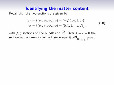
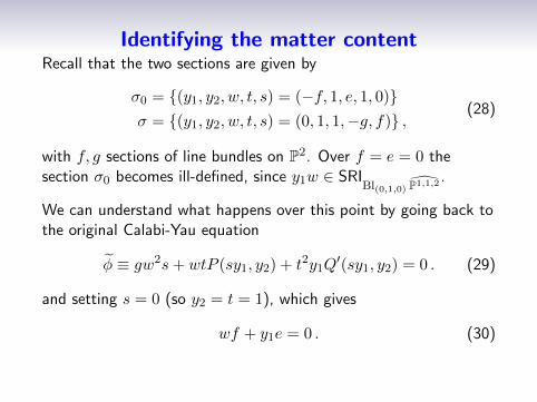
Identifying the matter contentRecall that the two sections are given by

σ0 = {(y1, y2, w, t, s) = (−f, 1, e, 1, 0)}σ = {(y1, y2, w, t, s) = (0, 1, 1,−g, f)} ,

with f, g sections of line bundles on P2. Over f = e = 0 thesection σ0 becomes ill-defined, since y1w ∈ SRI

Bl(0,1,0) P1,1,2 .

We can understand what happens over this point by going back tothe original Calabi-Yau equation

and setting s = 0 (so y2 = t = 1), which gives

wf + y1e = 0 . (30)

When f = e = 0 we have that (w, y1) are unconstrained, so thesection jumps in dimension.

Bl(0,1,0) P1,1,2 .

wf + y1e = 0 . (30)

Bl(0,1,0) P1,1,2 .

wf + y1e = 0 . (30)

Identifying the matter content

In addition, when f = e = 0, the Calabi-Yau equation factorizes as

s(gw2 + wty1P′(sy1, y2) + t2y2

1Q′′(sy1, y2)︸︷︷︸

) ≡ sΣ = 0 (31)

with P ′ = P/(sy1) and Q′′ = Q′/(sy1).

Identifying the matter content

We introduce a U(1) charge generator associated to the divisor

DU(1) = 2σ − 2σ0 − 4π∗c1(TB) + E , (32)

which induces a charge for the M2 brane wrappingCs ≡ {s = f = e = 0} given by

QU(1) = Cs · (2σ − 2σ0 − 12[x1] + [t]) = 4 (33)

Cs · σ = 1 (34)

Cs · σ0 = −1 (35)

Cs · [x1] = 0 (36)

Cs · [t] = 0 . (37)

Specific examples

(a, b) h1,1(X) h2,1(X) P H(12) H(14) H(21) H(23) H(30)

(0, 3) 3 111 18 144 18 0 0 0(1, 4) 3 123 10 140 10 0 0 0(2, 5) 3 141 4 128 4 0 0 0(0,−2) 4 57 3 64 3 55 15 6(0,−1) 4 60 6 76 6 52 12 3(0, 0) 4 67 9 90 9 45 9 1(0, 1) 4 78 12 106 12 34 6 0(0, 2) 4 93 15 124 15 19 3 0(1, 0) 4 68 2 72 2 56 8 3(1, 1) 4 76 4 86 4 48 6 1(1, 2) 4 88 6 102 6 36 4 0(1, 3) 4 104 8 120 8 20 2 0(2, 3) 4 104 2 90 2 38 2 0(2, 4) 4 121 3 108 3 21 1 0(3, 6) 3 165 0 108 0 0 0 0(0,−3) 6 60 0 − − − − −

Back to the general idea

We have seen that the 5d theory of a compactification withoutsection X can be constructed from a Higgsing of 14 states in the5d theory coming from a compactification with various sections.

We focus on Chern-Simons terms. The CS terms for X are wellunderstood by now [Grimm Kapfer Keitel, Grimm Hayashi], andfollowing them to the deformed side X is not hard.

The resulting Chern-Simons terms match perfectly those of a fluxed S1

reduction of a 6d theory with a massive U(1). [See Thomas’ talk formore details.]

The origin of the flux

The fact that it is a fluxed reduction is perhaps a little surprising.The following argument is originally by Witten.

The general metric of a fibration (with or without section) takesthe form

ds2 = gi duidu +

Imτ|X − τY |2 , (38)

X = dx+ X , Y = dy + Y . (39)

Whenever one has a section, one can choose coordinates such thatX = Y = 0, but this is not possible when the fibration has notsection, they become connection on a non-trivial bundle.

The origin of the flux

The fact that it is a fluxed reduction is perhaps a little surprising.The following argument is originally by Witten.

The general metric of a fibration (with or without section) takesthe form

ds2 = gi duidu +

Imτ|X − τY |2 , (38)

X = dx+ X , Y = dy + Y . (39)

Whenever one has a section, one can choose coordinates such thatX = Y = 0, but this is not possible when the fibration has notsection, they become connection on a non-trivial bundle.

The origin of the fluxThese cross terms give mixed components in the metric, andfollowing the F theory limit (reduction to IIA and T-duality), oneeasily sees that the effect of the off-diagonal components is theintroduction of a flux.Viewing x as the M-theory circle

ds2M = e4φIIA/3(dx+ CIIA

1 )2 + e−2φIIA/3ds2IIA . (40)

one reads

CIIA1 = Re τ dy + ReK , (41)

ds2IIA =

Imτ(Im τ dy + ImK)2 + gi du

with K = X − τ Y . Then T-dualizing along y

CIIB2 = X ∧ dy

BIIB2 = Y ∧ dy

}=⇒ (F3, H3) 6= (0, 0) . (43)

Conclusions

F-theory on spaces without section makes perfect sense. The5d theory reduction seems unconventional.

There is a nice family of examples closely related to exampleswith extra U(1)s.

But we also propose (in the paper, not discussed here) anintrinsic recipe, without the need of a conifold transition.

Some questions

The relation to [Morrison Braun, Morrison Taylor] is not totallyclear, although many ingredients seem suggestively related.

Compactifications to 4d are probably understandable too, and willlikely yield interesting structure.

Applications to pheno?

��

physics of f-theory compactifications without section · physics of f-theory compacti cations ......

Documents